The sphere packing problem indimension 8

Maryna S. Viazovska

April 5, 2017

In this paper we prove that no packing of unit balls in Euclidean space R8

has density greater than that of the E8-lattice packing.

Keywords: Sphere packing, Modular forms, Fourier analysisAMS subject classification: 52C17, 11F03, 11F30

1 Introduction

The sphere packing constant measures which portion of d-dimensional Euclidean spacecan be covered by non-overlapping unit balls. More precisely, let Rd be the Euclideanvector space equipped with distance ‖ · ‖ and Lebesgue measure Vol(·). For x ∈ Rd andr ∈ R>0 we denote by Bd(x, r) the open ball in Rd with center x and radius r. LetX ⊂ Rd be a discrete set of points such that ‖x−y‖ ≥ 2 for any distinct x, y ∈ X. Thenthe union

P =⋃x∈X

Bd(x, 1)

is a sphere packing. If X is a lattice in Rd then we say that P is a lattice sphere packing.The finite density of a packing P is defined as

∆P(r) :=Vol(P ∩Bd(0, r))

Vol(Bd(0, r)), r > 0.

We define the density of a packing P as the limit superior

∆P := lim supr→∞

∆P(r).

The number be want to know is the supremum over all possible packing densities

∆d := supP⊂Rd

sphere packing

∆P ,

1

arX

iv:1

603.

0424

6v2

[m

ath.

NT

] 4

Apr

201

7

called the sphere packing constant.For which dimensions do we know the exact value of ∆d? Trivially, in dimension 1

we have ∆1 = 1. It has long been known that a best packing in dimension 2 is thefamiliar hexagonal lattice packing, in which each disk is touching six others. The firstproof of this result was given by A. Thue at the beginning ot twentieth century [18].However, his proof was considered by some experts incomplete. A rigorous proof wasgiven by L. Fejes Toth in 1940s [10]. The density of the hexagonal lattice packingis π√

12, therefore ∆2 = π√

12≈ 0.90690. The packing problem in dimension 3 turned

out to be more difficult. Johannes Kepler conjectured in his essay “On the six-corneredsnowflake” (1611) that no arrangement of equally sized spheres filling space has densitygreater than π√

18. This density is attained by the face-centered cubic packing and also

by uncountably many non-lattice packings. The Kepler conjecture was famously provenby T. Hales in 1998 [11] and therefore we know that ∆3 = π√

18≈ 0.74048. In 2015 Hales

and his 21 coauthors published a complete formal proof of the Kepler conjecture that canbe verified by automated proof checking software. Before now, the exact values of thesphere packing constants in all dimensions greater than 3 have been unknown. A list ofconjectural best packings in dimensions less than 10 can be found in [6]. Upper boundsfor the sphere packing constants ∆d as d ≤ 36 are given in [4]. Surprisingly enough, theseupper bounds and known lower bounds on ∆d are extremely close in dimensions d = 8and d = 24.

The main result of this paper is the proof that

∆8 =π4

384≈ 0.25367.

This is the density of the E8-lattice sphere packing. Recall that the E8-lattice Λ8 ⊂ R8

is given by

Λ8 = {(xi) ∈ Z8 ∪ (Z + 12)8|

8∑i=1

xi ≡ 0 (mod 2)}.

Λ8 is the unique up to isometry positive-definite, even, unimodular lattice of rank 8.The name derives from the fact that it is the root lattice of the E8 root system. Theminimal distance between two points in Λ8 is

√2. The E8-lattice sphere packing is the

packing of unit balls with centers at 1√2Λ8. Our main result is

Theorem 1. No packing of unit balls in Euclidean space R8 has density greater thanthat of the E8-lattice packing.

Furthermore, our proof of Theorem 1 combined with arguments given in [4, Section 8]implies that the E8-lattice sphere packing is the unique periodic packing of maximaldensity.

The paper is organized as follows. In Section 2 we explain the idea of the proof ofTheorem 1 and describe the methods we use. In Section 3 we give a brief overview of thetheory of modular forms. In Section 4 we construct supplementary radial functions a,b : R8 → iR, which are eigenfunctions of the Fourier transform and have double zeroes at

2

almost all points of Λ8. This construction is crucial for our proof of Theorem 1. Finally,in Section 5 we complete the proof.

2 Linear programming bounds

Our proof of Theorem 1 is based on linear programming bounds. This technique wassuccessfully applied to obtain upper bounds in a wide range of discrete optimizationproblems such as error-correcting codes [7], equal weight quadrature formulas [8], andspherical codes [13, 16]. In exceptional cases linear programming bounds are optimal [5].However, in general linear programming bounds are not sharp and it is an open questionhow big the errors of such bounds can be. It is known [2] that the linear programmingbounds for the minimal number of points in an equal weight quadrature formula onthe sphere Sd are asymptotically optimal up to a constant depending on d. Linearprogramming bounds can also be applied to the sphere packing problem. Kabatianskyand Levenshtein [13] deduced upper bounds for sphere packing from their results onspherical codes.

In 2003 Cohn and Elkies [4] developed linear programming bounds that apply directlyto sphere packings. Using their new method they improved the previously known upperbounds for the sphere packing constant in dimensions from 4 to 36. The most strikingresults obtained by this technique are upper bounds for dimensions 8 and 24. Forexample, their upper bound for ∆8 was only 1.000001 times greater than the lowerbound, which is given by the density of the E8 sphere packing. This bound can beimproved even further by more extensive computer computations.

We explain the Cohn–Elkies linear programming bounds in more detail. To this endwe recall a few definitions from Fourier analysis. The Fourier transform of an L1 functionf : Rd → C is defined as

F(f)(y) = f(y) :=

∫Rd

f(x) e−2πix·y dx, y ∈ Rd

where x · y = 12‖x‖

2 + 12‖y‖

2 − 12‖x − y‖2 is the standard scalar product in Rd. A

C∞ function f : Rd → C is called a Schwartz function if it tends to zero as ‖x‖ → ∞faster then any inverse power of ‖x‖, and the same holds for all partial derivatives of f .The set of all Schwartz functions is called the Schwartz space. The Fourier transform isan automorphism of this space. We will also need the following wider class of functions.We say that a function f : Rd → C is admissible if there is a constant δ > 0 such that|f(x)| and |f(x)| are bounded above by a constant times (1 + |x|)−d−δ. The followingtheorem is the key result of [4]:

Theorem 2. (Cohn, Elkies [4]) Suppose that f : Rd → R is an admissible function, isnot identically zero, and satisfies:

f(x) ≤ 0 for ‖x‖ ≥ 1 (1)

3

andf(x) ≥ 0 for all x ∈ Rd. (2)

Then the density of d-dimensional sphere packings is bounded above by

f(0)

f(0)· π

d2

2d Γ(d2 + 1)=f(0)

f(0)·VolBd(0,

1

2).

Without loss of generality we can assume that a function f in Theorem 2 is radial,i. e. its value at each point depends only on the distance between the point and theorigin [4, p. 695]. For a radial function f0 : Rd → R we will denote by f0(r) the commonvalue of f0 on vectors of length r. Henceforth we assume d = 8. The Poisson summationformula implies ∑

`∈ 1√2

Λ8

f(`) = 24∑

`∈√

2Λ8

f(`).

Hence, if a function f satisfies conditions (1) and (2) then

f(0)

f(0)≥ 24.

We say that an admissible function f : R8 → R is optimal if it satisfies (1), (2) andf(0)/f(0) = 24.

The main step in our proof of Theorem 1 is the explicit construction of an optimalfunction. It will be convenient for us to scale this function by

√2.

Theorem 3. There exists a radial Schwartz function g : R8 → R which satisfies:

g(x) ≤ 0 for ‖x‖ ≥√

2, (3)

g(x) ≥ 0 for all x ∈ R8, (4)

g(0) = g(0) = 1. (5)

Moreover, the values g(x) and g(x) do not vanish for all vectors x with ‖x‖2 /∈ 2Z>0.

Theorem 2 applied to the optimal function f(x) = g(√

2x) immediately implies The-orem 1. Additionally, the function g satisfies the conclusions of [4, Conjecture 8.1]. Thisimplies the uniqueness of the densest periodic sphere packing in R8.

Let us briefly explain our strategy for the proof of Theorem 3. First, we observethat conditions (3)–(5) imply additional properties of the function g. Suppose thatthere exists a Schwartz function g such that the conditions (3)–(5) hold. The Poissonsummation formula states ∑

`∈Λ8

g(`) =∑`∈Λ8

g(`). (6)

Since ‖`‖ ≥√

2 for all ` ∈ Λ8\{0}, conditions (3) and (5) imply∑`∈Λ8

g(`) ≤ g(0) = 1. (7)

4

On the other hand, conditions (4) and (5) imply∑`∈Λ8

g(`) ≥ g(0) = 1. (8)

Therefore, we deduce that g(`) = g(`) = 0 for all ` ∈ Λ8\{0}. Moreover, the firstderivatives d

drg(r) and ddr g(r) also vanish at all Λ8-lattice points of length bigger than√

2. We will say that g and g have double zeroes at these points. This property givesus a hint on constructing the function g explicitly.

In Section 5 a function g satisfying (3)–(5) is given in a closed form. Namely, it isdefined as an integral transform (Laplace transform) of a modular form of a certain kind.The next section is a brief introduction to the theory of modular forms.

3 Modular forms

Let H be the upper half-plane {z ∈ C | Im (z) > 0}. The modular group Γ(1) := PSL2(Z)acts on H by linear fractional transformations(

a bc d

)z :=

az + b

cz + d.

Let N be a positive integer. The level N principal congruence subgroup of Γ(1) is

Γ(N) :={(

a bc d

)∈ Γ(1)

∣∣ ( a bc d

)≡ ( 1 0

0 1 ) mod N}.

A subgroup Γ ⊂ Γ(1) is called a congruence subgroup if Γ(N) ⊂ Γ for some N ∈ N. Animportant example of a congruence subgroup is

Γ0(N) :={(

a bc d

)∈ Γ(1)

∣∣ c ≡ 0 mod N}.

Let z ∈ H, k ∈ Z, and(a bc d

)∈ SL2(Z). The automorphy factor of weight k is defined

asjk(z,

(a bc d

)) := (cz + d)−k.

The automorphy factor satisfies the chain rule

jk(z, γ1γ2) = jk(z, γ2) jk(γ2z, γ1).

Let F be a function on H and γ ∈ PSL2(Z). Then the slash operator acts on F by

(F |kγ)(z) := jk(z, γ)F (γz).

The chain rule impliesF |kγ1γ2 = (F |kγ1)|kγ2.

A (holomorphic) modular form of integer weight k and congruence subgroup Γ is aholomorphic function f : H→ C such that:

5

1. f |kγ = f for all γ ∈ Γ and

2. for each α ∈ Γ(1) the function f |kα has Fourier expansion

f |kα(z) =∞∑n=0

cf (α,n

nα) e2πi n

nαz

for some nα ∈ N and Fourier coefficients cf (α,m) ∈ C.

Let Mk(Γ) be the space of modular forms of weight k for the congruence subgroup Γ.A key fact in the theory of modular forms is that the spaces Mk(Γ) are finite dimensional.

We consider several examples of modular forms. For an even integer k ≥ 4 we definethe weight k Eisenstein series as

Ek(z) :=1

2ζ(k)

∑(c,d)∈Z2\(0,0)

(cz + d)−k. (9)

Since the sum converges absolutely, it is easy to see that Ek ∈Mk(Γ(1)). The Eisensteinseries possesses the Fourier expansion

Ek(z) = 1 +2

ζ(1− k)

∞∑n=1

σk−1(n) e2πinz, (10)

where σk−1(n) =∑

d|n dk−1. In particular, we have

E4(z) = 1 + 240∞∑n=1

σ3(n) e2πinz,

E6(z) = 1− 504

∞∑n=1

σ5(n) e2πinz.

The infinite sum (9) does not converge absolutely for k = 2. On the other hand,the expression (10) converges to a holomorphic function on the upper half-plane andtherefore we set

E2(z) := 1− 24

∞∑n=1

σ1(n) e2πinz. (11)

This function is not modular, but it satisfies

z−2E2

(−1

z

)= E2(z)− 6i

π

1

z. (12)

The proof of this identity can be found in [20, Section 2.3]. The weight two Eisensteinseries E2 is an example of a quasimodular form [20, Section 5.1].

6

Another example of modular forms we consider are theta functions [20, Section 3.1].We define three theta functions (so-called “Thetanullwerte”) as

θ00(z) =∑n∈Z

eπin2z,

θ01(z) =∑n∈Z

(−1)n eπin2z,

θ10(z) =∑n∈Z

eπi(n+ 12

)2z.

The group Γ(1) is generated by the elements T = ( 1 10 1 ) and S =

(0 1−1 0

). These elements

act on the fourth powers of the theta functions in the following way

z−2 θ400

(−1

z

)= − θ4

00(z), (13)

z−2 θ401

(−1

z

)= − θ4

10(z), (14)

z−2 θ410

(−1

z

)= − θ4

01(z), (15)

and

θ400(z + 1) = θ4

01(z), (16)

θ401(z + 1) = θ4

00(z), (17)

θ410(z + 1) = − θ4

10(z). (18)

Moreover, these three theta functions satisfy the Jacobi identity

θ401 + θ4

10 = θ400. (19)

The theta functions θ400, θ

401, and θ4

10 belong to M2(Γ(2)).A weakly-holomorphic modular form of integer weight k and congruence subgroup Γ

is a holomorphic function f : H→ C such that:

1. f |kγ = f for all γ ∈ Γ,

2. for each α ∈ Γ(1) the function f |kα has Fourier expansion

f |kα(z) =∞∑

n=n0

cf (α,n

nα) e2πi n

nαz

for some n0 ∈ Z and nα ∈ N.

For an m-periodic holomorphic function f and n ∈ 1mZ we will denote the n-th Fourier

coefficient of f by cf (n) so that

f(z) =∑n∈ 1

mZ

cf (n) e2πinz.

7

We denote the space of weakly-holomorphic modular forms of weight k and group Γ byM !k(Γ). The spaces M !

k(Γ) are infinite dimensional. Probably the most famous weakly-holomorphic modular form is the elliptic j-invariant

j :=1728E3

4

E34 − E2

6

.

This function belongs to M !0(Γ(1)) and has the Fourier expansion

j(z) = q−1 + 744 + 196884 q + 21493760 q2 + 864299970 q3 + 20245856256 q4 +O(q5)

where q = e2πiz. Using a simple computer algebra system such as PARI GP or Mathe-matica one can compute the first hundred terms of this Fourier expansion within a fewseconds. An important question is to find an asymptotic formula for cj(n), the n-thFourier coefficient of j. Using the Hardy-Ramanujan circle method [17, p. 460 – 461] orthe non-holomorphic Poincare series [15] one can show that

cj(n) =2π√n

∞∑k=1

Ak(n)

kI1

(4π√n

k

)n ∈ Z>0 (20)

whereAk(n) =

∑h mod k(h,k)=1

e−2πik

(nh+h′), hh′ ≡ −1(mod k),

and Iα(x) denotes the modified Bessel function of the first kind defined as in [1, Sec-tion 9.6]. A similar convergent asymptotic expansion holds for the Fourier coefficients ofany weakly holomorphic modular form [12, p.660 – 662], [3, Propositions 1.10 and 1.12].Such a convergent expansion implies effective estimates for the Fourier coefficients.

For a comprehensive introduction to the theory of modular forms we refer the readerto [20] and [9].

4 Fourier eigenfunctions with double zeroes at latticepoints

In this section we construct two radial Schwartz functions a, b : R8 → iR such that

F(a) = a (21)

F(b) = −b (22)

which double zeroes at all Λ8-vectors of length greater than√

2. Recall that each vectorof Λ8 has length

√2n for some n ∈ N≥0. We define a and b so that their values are purely

imaginary because this simplifies some of our computations. We will show in Section 5that an appropriate linear combination of functions a and b satisfies conditions (3)–(5).

8

First, we will define the function a. To this end we consider the following weaklyholomorphic modular forms:

ϕ−2 :=−1728E4E6

E34 − E2

6

, (23)

ϕ−4 :=1728E2

4

E34 − E2

6

. (24)

The modular form E34 −E2

6 does not vanish in the upper half-plain, hence ϕ−2 and ϕ−4

have no poles in H. Analogously to (20), the Fourier coefficients of ϕ−2 and ϕ−4 satisfy

cϕκ(n) = 2π nκ−12

∞∑k=1

Ak(n)

kI1−κ

(4π√n

k

)n ∈ Z>0, κ = −2,−4. (25)

We define

φ−4 :=ϕ−4, (26)

φ−2 :=ϕ−4E2 + ϕ−2, (27)

φ0 :=ϕ−4E22 + 2ϕ−2E2 + j − 1728. (28)

The function φ0(z) is not modular; however the identity (12) implies the following trans-formation rule:

φ0

(−1

z

)= φ0(z)− 12i

π

1

zφ−2(z)− 36

π2

1

z2φ−4(z). (29)

Moreover, we have

φ−2 = − 3D(ϕ−4) + 3ϕ−2, (30)

φ0 = 12D2(ϕ−4)− 36D(ϕ−2) + 24j − 17856, (31)

where Df(z) = 12πi

ddzf(z). These identities combined with (20) and (25) give the asymp-

totic formula for the Fourier coefficients cφ−4(n), cφ−2(n), and cφ0(n). The first severalterms of the corresponding Fourier expansions are

φ−4(z) = q−1 + 504 + 73764 q + 2695040 q2 + 54755730 q3 +O(q4), (32)

φ−2(z) = 720 + 203040 q + 9417600 q2 + 223473600 q3 + 3566782080 q4 +O(q5), (33)

φ0(z) = 518400 q + 31104000 q2 + 870912000 q3 + 15697152000 q4 +O(q5), (34)

where q = e2πiz. For x ∈ R8 we define

a(x) :=

i∫−1

φ0

( −1

z + 1

)(z + 1)2 eπi‖x‖

2z dz +

i∫1

φ0

( −1

z − 1

)(z − 1)2 eπi‖x‖

2z dz (35)

−2

i∫0

φ0

(−1

z

)z2 eπi‖x‖

2z dz + 2

i∞∫i

φ0(z) eπi‖x‖2z dz.

9

We observe that the contour integrals in (35) converge absolutely and uniformly forx ∈ R8. Indeed, φ0(z) = O(e−2πiz) as Im (z)→∞. Therefore, a(x) is well defined. Nowwe prove that a satisfies condition (21).

Proposition 1. The function a defined by (35) belongs to the Schwartz space and sat-isfies

a(x) = a(x).

Proof. First, we prove that a is a Schwartz function. From (20), (25), and (31) wededuce that the Fourier coefficients of φ0 satisfy

|cφ0(n)| ≤ 2 e4π√n n ∈ Z>0.

Thus, there exists a positive constant C such that

|φ0(z)| ≤ C e−2πIm z for Im z >1

2.

We estimate the first summand in the right-hand side of (35). For r ∈ R≥0 we have

∣∣∣∣∣i∫

−1

φ0

( −1

z + 1

)(z + 1)2 eπir

2z dz

∣∣∣∣∣ =

∣∣∣∣∣−1/(i+1)∫i∞

φ0(z) z−4 eπir2(−1/z−1) dz

∣∣∣∣∣ ≤C1

∞∫1/2

e−2πt e−πr2/t dt ≤ C1

∞∫0

e−2πt e−πr2/t dt = C2 rK1(2

√2π r)

where C1 and C2 are some positive constants and Kα(x) is the modified Bessel functionof the second kind defined as in [1, Section 9.6]. This estimate also holds for the secondand third summand in (35). For the last summand we have∣∣∣∣∣

i∞∫i

φ0(z) eπir2z dz

∣∣∣∣∣ ≤ C∞∫

1

e−2πt e−πr2t dt = C3

eπ(r2+2)

r2 + 2.

Therefore, we arrive at

|a(r)| ≤ 4C2 rK1(2√

2πr) + 2C3e−π(r2+2)

r2 + 2.

It is easy to see that the left hand side of this inequality decays faster then any inversepower of r. Analogous estimates can be obtained for all derivatives dk

drka(r).

Now we show that a is an eigenfunction of the Fourier transform. We recall that theFourier transform of a Gaussian function is

F(eπi‖x‖2z)(y) = z−4 eπi‖y‖

2 (−1z

). (36)

10

Next, we exchange the contour integration with respect to z variable and Fourier trans-form with respect to x variable in (35). This can be done, since the corresponding doubleintegral converges absolutely. In this way we obtain

a(y) =

i∫−1

φ0

( −1

z + 1

)(z + 1)2 z−4 eπi‖y‖

2 (−1z

) dz +

i∫1

φ0

( −1

z − 1

)(z − 1)2 z−4 eπi‖y‖

2 (−1z

) dz

−2

i∫0

φ0

(−1

z

)z2 z−4 eπi‖y‖

2 (−1z

) dz + 2

i∞∫i

φ0(z) z−4 eπi‖y‖2 (−1

z) dz.

Now we make a change of variables w = −1z . We obtain

a(y) =

i∫1

φ0

(1− 1

w − 1

)(−1

w+ 1)2w2 eπi‖y‖

2 w dw

+

i∫−1

φ0

(1− 1

w + 1

)(−1

w− 1)2w2 eπi‖y‖

2 w dw

−2

i∫i∞

φ0(w) eπi‖y‖2 w dw + 2

0∫i

φ0

(−1

w

)w2 eπi‖y‖

2 w dw.

Since φ0 is 1-periodic we have

a(y) =

i∫1

φ0

( −1

z − 1

)(z − 1)2 eπi‖y‖

2 z dz +

i∫−1

φ0

( −1

z + 1

)(z + 1)2 eπi‖y‖

2 z dz

+2

i∞∫i

φ0(z) eπi‖y‖2 z dz − 2

i∫0

φ0

(−1

z

)z2 eπi‖y‖

2 z dz

= a(y).

This finishes the proof of the proposition.

Next, we check that a has double zeroes at all Λ8-lattice points of length greater then√2.

Proposition 2. For r >√

2 we can express a(r) in the following form

a(r) = −4 sin(πr2/2)2

i∞∫0

φ0

(−1

z

)z2 eπir

2 z dz. (37)

11

Proof. We denote the right hand side of (37) by d(r). It is easy to see that d(r) is well-defined. Indeed, from the transformation formula (29) and the expansions (34)–(32) weobtain

φ0

(−1

it

)=O(e−2π/t) as t→ 0

φ0

(−1

it

)=O(t−2 e2πt) as t→∞

Hence, the integral (37) converges absolutely for r >√

2. We can write

d(r) =

i∞−1∫−1

φ0

( −1

z + 1

)(z + 1)2 eπir

2 z dz − 2

i∞∫0

φ0

(−1

z

)z2 eπir

2 z dz

+

i∞+1∫1

φ0

( −1

z − 1

)(z − 1)2 eπir

2 z dz.

From (29) we deduce that if r >√

2 then φ0

(−1z

)z2 eπir

2 z → 0 as Im (z)→∞. There-

fore, we can deform the paths of integration and rewrite

d(r) =

i∫−1

φ0

( −1

z + 1

)(z + 1)2 eπir

2 z dz +

i∞∫i

φ0

( −1

z + 1

)(z + 1)2 eπir

2 z dz

−2

i∫0

φ0

(−1

z

)z2 eπir

2 z dz − 2

i∞∫i

φ0

(−1

z

)z2 eπir

2 z dz

+

i∫1

φ0

( −1

z − 1

)(z − 1)2 eπir

2 z dz +

i∞∫i

φ0

( −1

z − 1

)(z − 1)2 eπir

2 z dz.

Now from (29) we find

φ0

( −1

z + 1

)(z + 1)2 − 2φ0

(−1

z

)z2 + φ0

( −1

z − 1

)(z − 1)2 =

φ0(z + 1) (z + 1)2 − 2φ0(z) z2 + φ0(z − 1) (z − 1)2

− 12i

π

(φ−2(z + 1) (z + 1)− 2φ−2(z) z + φ−2(z − 1) (z − 1)

)− 36

π2

(φ−4(z + 1)− 2φ−4(z) + φ−4(z − 1)

)=

2φ0(z).

12

Thus, we obtain

d(r) =

i∫−1

φ0

( −1

z + 1

)(z + 1)2 eπir

2 z dz − 2

i∫0

φ0

(−1

z

)z2 eπir

2 z dz

+

i∫1

φ0

( −1

z − 1

)(z − 1)2 eπir

2 z dz + 2

i∞∫i

φ0(z) eπir2 z dz = a(r).

This finishes the proof.

Finally, we find another convenient integral representation for a and compute valuesof a(r) at r = 0 and r =

√2.

Proposition 3. For r ≥ 0 we have

a(r) =4i sin(πr2/2)2

(36

π3 (r2 − 2)− 8640

π3 r4+

18144

π3 r2(38)

+

∞∫0

(t2 φ0

( it

)− 36

π2e2πt +

8640

πt− 18144

π2

)e−πr

2t dt

).

The integral converges absolutely for all r ∈ R≥0.

Proof. Suppose that r >√

2. Then by Proposition 2

a(r) = 4i sin(πr2/2)2

∞∫0

φ0(i/t) t2 e−πr2t dt.

From (34)–(29) we obtain

φ0(i/t) t2 =36

π2e2πt − 8640

πt+

18144

π2+O(t2 e−2πt) as t→∞. (39)

For r >√

2 we have

∞∫0

(36

π2e2πt +

8640

πt+

18144

π2

)e−πr

2t dt =36

π3 (r2 − 2)− 8640

π3 r4+

18144

π3 r2. (40)

Therefore, the identity (38) holds for r >√

2.On the other hand, from the definition (35) we see that a(r) is analytic in some

neighborhood of [0,∞). The asymptotic expansion (39) implies that the right hand sideof (38) is also analytic in some neighborhood of [0,∞). Hence, the identity (38) holdson the whole interval [0,∞). This finishes the proof of the proposition.

13

From the identity (38) we see that the values a(r) are in iR for all r ∈ R≥0. Inparticular, we have

Proposition 4. We have

a(0) =−i 8640

πa(√

2) = 0 a′(√

2) =i 72√

2

π. (41)

Proof. These identities follow immediately from the previous proposition.

Now we construct function b. To this end we consider the modular form

h := 128θ4

00 + θ401

θ810

. (42)

It is easy to see that h ∈ M !−2(Γ0(2)). Indeed, first we check that h|−2γ = h for all

γ ∈ Γ0(2). Since the group Γ0(2) is generated by elements ( 1 02 1 ) and ( 1 1

0 1 ) it suffices tocheck that h is invariant under their action. This follows immediately from (13)–(18)and (42). Next we analyze the poles of h. It is known [14, Chapter I Lemma 4.1] thatθ10 has no zeros in the upper-half plane and hence h has poles only at the cusps. At thecusp i∞ this modular form has the Fourier expansion

h(z) = q−1 + 16− 132q + 640q2 − 2550q3 +O(q4).

Let I = ( 1 00 1 ), T = ( 1 1

0 1 ), and S =(

0 −11 0

)be elements of Γ(1). We define the following

three functions

ψI :=h− h|−2ST, (43)

ψT :=ψI |−2T, (44)

ψS :=ψI |−2S. (45)

More explicitly, we have

ψI = 128θ4

00 + θ401

θ810

+ 128θ4

01 − θ410

θ800

, (46)

ψT = 128θ4

00 + θ401

θ810

+ 128θ4

00 + θ410

θ801

, (47)

ψS = − 128θ4

00 + θ410

θ801

− 128θ4

10 − θ401

θ800

. (48)

The Fourier expansions of these functions are

ψI(z) = q−1 + 144− 5120q1/2 + 70524q − 626688q3/2 + 4265600q2 +O(q5/2), (49)

ψT (z) = q−1 + 144 + 5120q1/2 + 70524q + 626688q3/2 + 4265600q2 +O(q5/2), (50)

ψS(z) = − 10240q1/2 − 1253376q3/2 − 48328704q5/2 − 1059078144q7/2 +O(q9/2). (51)

14

For x ∈ R8 define

b(x) :=

i∫−1

ψT (z) eπi‖x‖2z dz +

i∫1

ψT (z) eπi‖x‖2z dz (52)

−2

i∫0

ψI(z) eπi‖x‖2z dz − 2

i∞∫i

ψS(z) eπi‖x‖2z dz.

Now we prove that b satisfies condition (22).

Proposition 5. The function b defined by (52) belongs to the Schwartz space and sat-isfies

b(x) = −b(x).

Proof. Here, we repeat the arguments used in the proof of Proposition 1. First we showthat b is a Schwartz function. We have

i∫−1

ψT (z) eπir2z dz =

i+1∫0

ψI(z) eπir2(z−1) dz =

−1/(i+1)∫i∞

ψI

(−1

z

)eπir

2(−1/z−1) z−2 dz =

−1/(i+1)∫i∞

ψS(z) z−4 eπir2(−1/z−1) dz.

There exists a positive constant C such that

|ψS(z)| ≤ C e−π Im z for Im z >1

2.

Thus, as in the proof of Proposition 1 we estimate the first summand in the left-handside of (52) ∣∣∣∣∣

i∫−1

ψT (z) eπir2z dz

∣∣∣∣∣ ≤ C1 rK1(2πr).

We combine this inequality with analogous estimates for the other three summands andobtain

|b(r)| ≤ C2 rK1(2πr) + C3e−π(r2+1)

r2 + 1.

Here C1, C2, and C3 are some positive constants. Similar estimates hold for all deriva-tives dk

dkrb(r).

15

Now we prove that b is an eigenfunction of the Fourier transform. We use identity (36)and interchange contour integration in z and Fourier transform in x. Thus we obtain

F(b)(x) =

i∫−1

ψT (z) z−4 eπi‖x‖2(−1

z) dz +

i∫1

ψT (z) z−4 eπi‖x‖2(−1

z) dz

−2

i∫0

ψI(z) z−4 eπi‖x‖

2(−1z

) dz − 2

i∞∫i

ψS(z) z−4 eπi‖x‖2(−1

z) dz.

We make the change of variables w = −1z and arrive at

F(b)(x) =

i∫1

ψT

(−1

w

)w2 eπi‖x‖

2w dw +

i∫−1

ψT

(−1

w

)w2 eπi‖x‖

2w dw

−2

i∫i∞

ψI

(−1

w

)w2 eπi‖x‖

2w dw − 2

0∫i

ψS

(−1

w

)w2 eπi‖x‖

2w dw.

Now we observe that the definitions (43)–(45) imply

ψT |−2S =− ψT ,ψI |−2S =ψS ,

ψS |−2S =ψI .

Therefore, we arrive at

F(b)(x) =

i∫1

−ψT (z) eπi‖x‖2z dz +

i∫−1

−ψT (z) eπi‖x‖2z dz

+2

i∞∫i

ψS(z) eπi‖x‖2z dz + 2

i∫0

ψI(z) eπi‖x‖2w dw.

Now from (52) we see thatF(b)(x) = −b(x).

Now we regard the radial function b as a function on R≥0. We check that b has doubleroots at Λ8-points.

Proposition 6. For r >√

2 function b(r) can be expressed as

b(r) = −4 sin(πr2/2)2

i∞∫0

ψI(z) eπir2 z dz. (53)

16

Proof. We denote the right hand side of (53) by c(r). First, we check that c(r) iswell-defined. We have

ψI(it) = O(t2 e−π/t) as t→ 0,

ψI(it) = O(e2πt) as t→∞.

Therefore, the integral (53) converges for r >√

2. Then we rewrite it in the followingway:

c(r) =

i∞−1∫−1

ψI(z + 1) eπir2 z dz − 2

i∞∫0

ψI(z) eπir2 z dz +

i∞+1∫1

ψI(z − 1) eπir2 z dz.

From the Fourier expansion (49) we know that ψI(z) = e−2πiz + O(1) as Im (z) → ∞.By assumption r2 > 2, hence we can deform the path of integration and write

i∞−1∫−1

ψI(z + 1) eπir2 z dz =

i∫−1

ψT (z) eπir2 z dz +

i∞∫i

ψT (z) eπir2 z dz, (54)

i∞+1∫1

ψI(z − 1) eπir2 z dz =

i∫−1

ψT (z) eπir2 z dz +

i∞∫i

ψT (z) eπir2 z dz. (55)

We have

c(r) =

i∫−1

ψT (z) eπir2 z dz +

i∫1

ψT (z) eπir2 z dz − 2

i∫0

ψI(z) eπir2 z dz (56)

+ 2

i∞∫i

(ψT (z)− ψI(z)) eπir2 z dz.

Next, we check that the functions ψI , ψT , and ψS satisfy the following identity:

ψT + ψS = ψI . (57)

Indeed, from definitions (43)-(45) we get

ψT + ψS =(h− h|−2ST )|−2T + (h− h|−2ST )|−2S

=h|−2T − h|−2ST2 + h|−2S − h|−2STS.

Note that ST 2S belongs to Γ0(2). Thus, since h ∈M !−2Γ0(2) we get

ψT + ψS = h|−2T − h|−2STS.

Now we observe that T and STS(ST )−1 are also in Γ0(2). Therefore,

ψT + ψS = h|−2T − h|−2STS = h− h|−2ST = ψI .

17

Combining (56) and (57) we find

c(r) =

i∫−1

ψT (z) eπir2 z dz +

i∫1

ψT (z) eπir2 z dz − 2

i∫0

ψI(z) eπir2 z dz

− 2

i∞∫i

ψS(z) eπir2 z dz

=b(r).

At the end of this section we find another integral representation of b(r) for r ∈ R≥0

and compute special values of b.

Proposition 7. For r ≥ 0 we have

b(r) = 4i sin(πr2/2)2

144

π r2+

1

π (r2 − 2)+

∞∫0

(ψI(it)− 144− e2πt

)e−πr

2t dt

. (58)

The integral converges absolutely for all r ∈ R≥0.

Proof. The proof is analogous to the proof of Proposition 3. First, suppose that r >√

2.Then by Proposition 6

b(r) = 4i sin(πr2/2)2

∞∫0

ψI(it) e−πr2t dt.

From (49) we obtain

ψI(it) = e2πt + 144 +O(e−πt) as t→∞. (59)

For r >√

2 we have

∞∫0

(e2πt + 144

)e−πr

2t dt =1

π (r2 − 2)+

144

π r2. (60)

Therefore, the identity (38) holds for r >√

2.On the other hand, from the definition (52) we see that b(r) is analytic in some

neighborhood of [0,∞). The asymptotic expansion (59) implies that the right hand sideof (58) is also analytic in some neighborhood of [0,∞). Hence, the identity (58) holdson the whole interval [0,∞). This finishes the proof of the proposition.

We see from (58) that b(r) ∈ iR far all r ∈ R≥0. Another immediate corollary of thisproposition is

Proposition 8. We have

b(0) = 0 b(√

2) = 0 b′(√

2) = 2√

2π i. (61)

18

5 Proof of Theorem 3

Finally, we are ready to prove Theorem 3.

Theorem 4. The function

g(x) :=π i

8640a(x) +

i

240πb(x)

satisfies conditions (3)–(5). Moreover, the values g(x) and g(x) do not vanish for allvectors x with ‖x‖2 /∈ 2Z>0.

Proof. First, we prove that (3) holds. By Propositions 2 and 6 we know that for r >√

2

g(r) =π

2160sin(πr2/2)2

∞∫0

A(t) e−πr2t dt (62)

where

A(t) = −t2φ0(i/t)− 36

π2ψI(it).

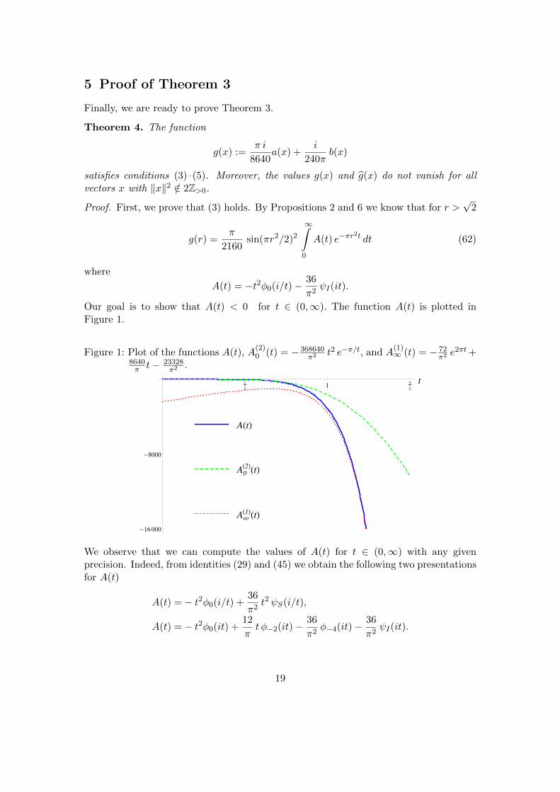
Our goal is to show that A(t) < 0 for t ∈ (0,∞). The function A(t) is plotted inFigure 1.

Figure 1: Plot of the functions A(t), A(2)0 (t) = −368640

π2 t2 e−π/t, and A(1)∞ (t) = − 72

π2 e2πt+

8640π t− 23328

π2 .

AHtL

A0H2LHtL

A¥H1LHtL

1

21

3

2

t

-8000

-16 000

We observe that we can compute the values of A(t) for t ∈ (0,∞) with any givenprecision. Indeed, from identities (29) and (45) we obtain the following two presentationsfor A(t)

A(t) =− t2φ0(i/t) +36

π2t2 ψS(i/t),

A(t) =− t2φ0(it) +12

πt φ−2(it)− 36

π2φ−4(it)− 36

π2ψI(it).

19

For an integer n ≥ 0 let A(n)0 and A

(n)∞ be the functions such that

A(t) =A(n)0 (t) +O(t2 e−πn/t) as t→ 0, (63)

A(t) =A(n)∞ (t) +O(t2 e−πnt) as t→∞. (64)

For each n ≥ 0 we can compute these functions from the Fourier expansions (34)–(32),(49), and (51). For example, from (32)–(34) and (49) we compute

A(6)∞ (t) =− 72

π2 e2πt−23328

π2 +184320π2 e−πt−5194368

π2 e−2πt+22560768

π2 e−3πt−250583040π2 e−4πt+

869916672π2 e−5πt

+t(8640π +

2436480π e−2πt+

113011200π e−4πt)−t2(518400 e−2πt+31104000 e−4πt).

From (32)–(34) and (51) we compute

A(6)0 (t) = t2(−368640

π2 e−π/t−518400 e−2π/t−45121536π2 e−3π/t−31104000 e−4π/t−1739833344

π2 e−5π/t).

Moreover, from the convergent asymptotic expansion for the Fourier coefficients of aweakly holomorphic modular form [3, Proposition 1.12] we find that the n-th Fouriercoefficient cψI (n) of ψI satisfies

|cψI (n)| ≤ e4π√n n ∈ 1

2Z>0. (65)

Similar inequalities hold for the Fourier coefficients of ψS , φ0, φ−2, and φ−4:

|cψS (n)| ≤ 2e4π√n n ∈ 1

2Z>0, (66)

|cφ0(n)| ≤ 2e4π√n n ∈ Z>0, (67)

|cφ−2(n)| ≤ e4π√n n ∈ Z>0, (68)

|cφ−4(n)| ≤ e4π√n n ∈ Z>0. (69)

Therefore, we can estimate the error terms in the asymptotic expansions (63) and (64)of A(t) ∣∣∣A(t)−A(m)

0 (t)∣∣∣ ≤(t2 +

36

π2)∞∑n=m

2e2√

2π√n e−πn/t,

∣∣∣A(t)−A(m)∞ (t)

∣∣∣ ≤(t2 +12

πt+

36

π2)

∞∑n=m

2e2√

2π√n e−πnt.

For an integer m ≥ 0 we set

R(m)0 :=(t2 +

36

π2)∞∑n=m

2e2√

2π√n e−πn/t,

R(m)∞ :=(t2 +

12

πt+

36

π2)

∞∑n=m

2e2√

2π√n e−πnt.

20

Using interval arithmetic we check that∣∣∣R(6)0 (t)

∣∣∣ ≤ ∣∣∣A(6)0 (t)

∣∣∣ for t ∈ (0, 1],∣∣∣R(6)∞ (t)

∣∣∣ ≤ ∣∣∣A(6)∞ (t)

∣∣∣ for t ∈ [1,∞),

A(6)0 (t) < 0 for t ∈ (0, 1],

A(6)∞ (t) < 0 for t ∈ [1,∞).

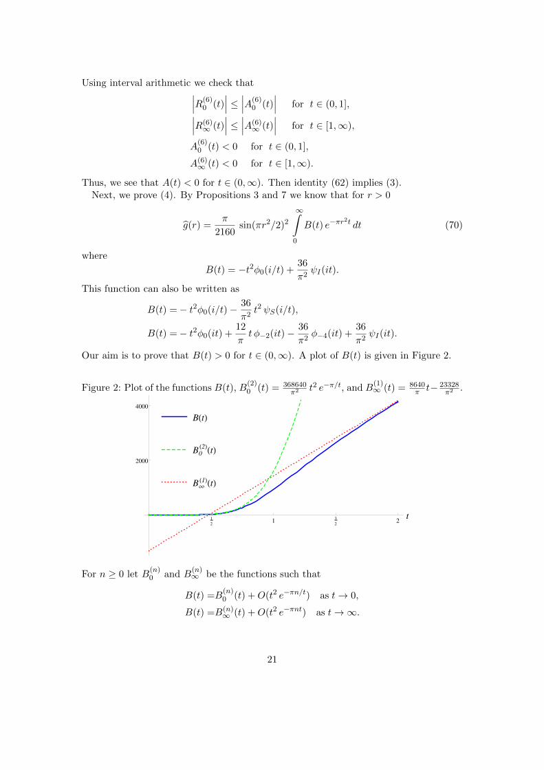
Thus, we see that A(t) < 0 for t ∈ (0,∞). Then identity (62) implies (3).Next, we prove (4). By Propositions 3 and 7 we know that for r > 0

g(r) =π

2160sin(πr2/2)2

∞∫0

B(t) e−πr2t dt (70)

where

B(t) = −t2φ0(i/t) +36

π2ψI(it).

This function can also be written as

B(t) =− t2φ0(i/t)− 36

π2t2 ψS(i/t),

B(t) =− t2φ0(it) +12

πt φ−2(it)− 36

π2φ−4(it) +

36

π2ψI(it).

Our aim is to prove that B(t) > 0 for t ∈ (0,∞). A plot of B(t) is given in Figure 2.

Figure 2: Plot of the functions B(t), B(2)0 (t) = 368640

π2 t2 e−π/t, and B(1)∞ (t) = 8640

π t− 23328π2 .

BHtL

B0H2LHtL

B¥

H1LHtL

1

21

3

22

t

2000

4000

For n ≥ 0 let B(n)0 and B

(n)∞ be the functions such that

B(t) =B(n)0 (t) +O(t2 e−πn/t) as t→ 0,

B(t) =B(n)∞ (t) +O(t2 e−πnt) as t→∞.

21

We find

B(6)∞ (t) =− 12960

π2 − 184320π2 e−πt − 116640

π2 e−2πt − 22560768π2 e−3πt + 56540160

π2 e−4πt − 869916672π2 e−5πt

+ t(8640π + 2436480

π e−2πt + 113011200π e−4πt)− t2(518400 e−2πt +31104000 e−4πt)

and

B(6)0 (t) = t2(368640

π2 e−π/t−518400 e−2π/t+45121536π2 e−3π/t−31104000 e−4π/t+1739833344

π2 e−5π/t).

The estimates (65)–(69) imply that∣∣∣B(t)−B(6)0 (t)

∣∣∣ ≤ R(6)0 (t) for t ∈ (0, 1]

and ∣∣∣B(t)−B(6)∞ (t)

∣∣∣ ≤ R(6)∞ (t) for t ∈ [1,∞).

Using interval arithmetic we verify that∣∣∣R(6)0 (t)

∣∣∣ ≤ ∣∣∣B(6)0 (t)

∣∣∣ for t ∈ (0, 1],∣∣∣R(6)∞ (t)

∣∣∣ ≤ ∣∣∣B(6)∞ (t)

∣∣∣ for t ∈ [1,∞),

B(6)0 (t) > 0 for t ∈ (0, 1],

B(6)∞ (t) > 0 for t ∈ [1,∞).

Now identity (70) implies (4).Finally, the property (5) readily follows from Proposition 4 and Proposition 8. This

finishes the proof of Theorems 4 and 3.

Acknowledgments

I thank Andriy Bondarenko for sharing his ideas, for fruitful discussions, and for hissupport. Also I am grateful to Danilo Radchenko for his valuable ideas and his helpwith numerical computations. I am most grateful to J. Kramer, J. M. Sullivan, G. M.Ziegler , and anonymous referees for their valuable comments and suggestions on themanuscript.

References

[1] M. Abramowitz, I. Stegun, Handbook of Mathematical Functions with For-mulas, Graphs, and Mathematical Tables, Applied Mathematics Series 55 (10thed.), New York, USA: United States Department of Commerce, National Bureau ofStandards; Dover Publications, 1964.

[2] A. Bondarenko, D. Radchenko, M. Viazovska, On optimal asymptoticbounds for spherical designs, Annals of Math. 178 (2)(2013), pp. 443–452.

22

[3] J. Bruinier, Borcherds products on O(2,l) and Chern classes of Heegner divisors,Springer Lecture Notes in Mathematics 1780 (2002).

[4] H. Cohn, N. Elkies, New upper bounds on sphere packings I, Annals of Math.157 (2003) pp. 689–714.

[5] H. Cohn, A. Kumar, Universally optimal distribution of points on spheres, J.Amer. Math. Soc. 20 (1) (2007), pp. 99–148.

[6] J. H. Conway and N. J. A. Sloane, What Are All the Best Sphere Packingsin Low Dimensions?, Discrete Comput. Geom. (Laszlo Fejes Toth Festschrift), 13(1995), pp. 383–403.

[7] P. Delsarte, Bounds for unrestricted codes, by linear programming, Philips Res.Rep. 27 (1972), pp. 272–289.

[8] P. Delsarte, J. M. Goethals, and J. J. Seidel, Spherical codes and designs,Geom. Dedicata, 6 (1977), pp. 363–388.

[9] F. Diamond, J. Shurman, A First Course in Modular Forms, Springer NewYork, 2005.

[10] L. Fejes Toth, Uber die dichteste Kugellagerung, Math. Z. 48 (1943), pp. 676–684.

[11] T. Hales, A proof of the Kepler conjecture, Annals of Math. 162 (3) (2005), pp.1065–1185.

[12] D. Hejhal, The Selberg trace formula for PSL(2,R), Vol. 2, Springer LectureNotes in Mathematics 1001 (1983).

[13] G. A. Kabatiansky and V. I. Levenshtein, Bounds for packings on a sphereand in space, Problems of Information Transmission 14 (1978), pp. 1–17.

[14] D. Mumford, Tata Lectures on Theta I, Birkhauser, 1983.

[15] H. Petersson, Ueber die Entwicklungskoeffizienten der automorphen Formen,Acta Mathematica, Bd. 58 (1932), pp. 169–215.

[16] F. Pfender, G. M. Ziegler, Kissing numbers, sphere packings, and some un-expected proofs, Notices of the AMS 51 (8) (2004) pp. 873–883.

[17] H. Rademacher and H. S. Zuckerman, On the Fourier coefficients of certainmodular forms of positive dimension, Annals of Math. (2) 39 (1938), pp. 433–462.

[18] A. Thue, Uber die dichteste Zusammenstellung von kongruenten Kreisen in einerEbene, Norske Vid. Selsk. Skr. No.1 (1910), pp. 1–9.

[19] V. A. Yudin, Lower bounds for spherical designs, Izv. Ross. Akad. Nauk Ser. Mat.61 (1997), pp. 211–233. English transl., Izv. Math. 6 (1997), pp. 673–683.

23

[20] D. Zagier, Elliptic Modular Forms and Their Applications, In: The 1-2-3 ofModular Forms, (K. Ranestad, ed.) Norway, Springer Universitext, 2008.

Berlin Mathematical School

Str. des 17. Juni 136

10623 Berlin

and

Humboldt University of Berlin

Rudower Chaussee 25

12489 Berlin

Email address: viazovska@gmail.com

24