3D Packing of Balls in DifferentContainers by VNS

A thesis submitted for the degree of

Doctor of Philosophy

by

Abdulaziz M. Alkandari

Supervisor

Nenad Mladenovic

Department Mathematical Sciences

School of Information Systems, Computing and Mathematics

Brunel University, London

June 2013

A

Abstract

In real world applications such as the transporting of goods products, packing is

a major issue. Goods products need to be packed such that the smallest space is

wasted to achieve the maximum transportation efficiency. Packing becomes more

challenging and complex when the product is circular/spherical. This thesis focuses

on the best way to pack three-dimensional unit spheres into the smallest spheri-

cal and cubical space. Unit spheres are considered in lieu of non-identical spheres

because the search mechanisms are more difficult in the latter set up and any im-

provements will be due to the search mechanism not to the ordering of the spheres.

The two-unit sphere packing problems are solved by approximately using a variable

neighborhood search (VNS) hybrid heuristic. A general search framework belonging

to the Artificial Intelligence domain, the VNS offers a diversification of the search

space by changing neighborhood structures and intensification by thoroughly in-

vestigating each neighborhood. It is flexible, easy to implement, adaptable to both

continuous and discrete optimization problems and has been use to solve a variety of

problems including large-sized real-life problems. Its runtime is usually lower than

other meta heuristic techniques. A tutorial on the VNS and its variants along with

recent applications and areas of applicability of each variant. Subsequently, this

thesis considers several variations of VNS heuristics for the two problems at hand,

discusses their individual efficiencies and effectiveness, their convergence rates and

studies their robustness. It highlights the importance of the hybridization which

yields near global optima with high precision and accuracy, improving many best-

known solutions indicate matching some, and improving the precision and accuracy

of others.

Keywords: variable neighborhood search, sphere packing, three-dimensional pack-

ing, meta heuristic, hybrid heuristics, multiple start heuristics.

Declaration of Originality

I hereby certify that the work presented in this thesis is my original research and

has not been presented for a higher degree at any other university or institute.

Signed: Dated:

Abdulaziz Alkandari

iv

Acknowledgements

First I would like to thank my God, whose response has always helped me and

given me the strength to complete my work. I express my heartfelt gratitude to all

those who made it possible for me to complete this thesis. I thank the Department

of Mathematics for providing me with the most recent programs in my research, for

giving me the requisite permissions to access the relevant articles in my work and

to use the departmental facilities.

I am deeply indebted to my supervisor, Dr. Nenad Mladenovic, whose help,

stimulating suggestions and encouragement helped me throughout my research as

well as the writing of this thesis.

I thank Dr. Rym M’Halah, for patiently explaining most of the software tools I

needed to deal with all of my different meshes and for cheering me on. I am also

grateful that she provided me with the FORTRAN code for the Variable Neighbour-

hood Search (VNS).

A sincere thank you goes to my friend Dr. Ahmad Alkandari for making sure the

English in this thesis reads smoothly and for providing many important tips and

suggestions, and also for always being there when I needed him. As luck would have

it, we wrote our thesis side by side, which I very much enjoyed.

I am grateful to my wife Safiah, who supported and encouraged me to complete

my thesis. I also dedicate this work to my children Alaa, Shaimaa, Dalya, and

v

Nasser. I am also grateful to my brothers, sisters, and my friends for their support

and prayers.

vi

Author’s Publications

1). M’Hallah R., Alkandari A., and Mladenovic N., Packing Unit Spheres into the

Smallest Sphere Using VNS and NLP, Computers & Operations Research 40 (2013)

603-615

2). M’Hallah R., and Alkandari A., Packing Unit Spheres into a Cube Using VNS,

Electronic Notes in Discrete Mathematics 39 (2012) 201-208

1

Contents

Abstract iii

Declaration iv

Acknowledgements v

Author’s Publications 1

List of Figures d

List of Tables e

1 Introduction 1

1.1 Background . . . . . . . . . . . . . . . . . . . . . . . . . . . . . . . . 1

1.2 Problem description . . . . . . . . . . . . . . . . . . . . . . . . . . . 2

1.3 Motivation . . . . . . . . . . . . . . . . . . . . . . . . . . . . . . . . 3

1.4 Contribution . . . . . . . . . . . . . . . . . . . . . . . . . . . . . . . 4

1.5 Outline . . . . . . . . . . . . . . . . . . . . . . . . . . . . . . . . . . 5

2 Variable Neighborhood Search 7

2.1 Introduction . . . . . . . . . . . . . . . . . . . . . . . . . . . . . . . . 7

2.2 Preliminaries . . . . . . . . . . . . . . . . . . . . . . . . . . . . . . . 9

a

2.2.1 The variable metric procedure . . . . . . . . . . . . . . . . . 10

2.2.2 Iterated local search (LS) . . . . . . . . . . . . . . . . . . . . 11

2.3 Elementary VNS algorithms . . . . . . . . . . . . . . . . . . . . . . . 14

2.3.1 The variable neighborhood descent . . . . . . . . . . . . . . . 15

2.3.2 The reduced variable neighborhood descent . . . . . . . . . . 17

2.3.3 The basic variable neighborhood search . . . . . . . . . . . . 19

2.3.4 The general variable neighborhood search . . . . . . . . . . . 20

2.3.5 The skewed variable neighborhood search . . . . . . . . . . . 22

2.3.6 The variable neighborhood decomposition search . . . . . . . 23

2.3.7 Comparison of the VNS variants . . . . . . . . . . . . . . . . 25

2.4 Parallel VNS . . . . . . . . . . . . . . . . . . . . . . . . . . . . . . . 26

2.5 Discussion and conclusion . . . . . . . . . . . . . . . . . . . . . . . . 32

3 Packing Unit Spheres into the Smallest Sphere Using the VNS and

NLP 33

3.1 Introduction . . . . . . . . . . . . . . . . . . . . . . . . . . . . . . . . 33

3.2 Literature review . . . . . . . . . . . . . . . . . . . . . . . . . . . . . 37

3.3 Proposed approach . . . . . . . . . . . . . . . . . . . . . . . . . . . . 41

3.3.1 Schittkowski’s local search . . . . . . . . . . . . . . . . . . . . 42

3.3.2 Variable neighborhood search . . . . . . . . . . . . . . . . . . 45

3.4 Computational results . . . . . . . . . . . . . . . . . . . . . . . . . . 48

3.4.1 Overall performance . . . . . . . . . . . . . . . . . . . . . . . 49

3.4.2 Feasibility of the initial solution . . . . . . . . . . . . . . . . . 52

3.4.3 Utility of the diversification strategies . . . . . . . . . . . . . 54

3.4.4 Utility of the VNS and the LS . . . . . . . . . . . . . . . . . 63

3.4.5 Comparison of the diversification strategies . . . . . . . . . . 66

3.5 Conclusion . . . . . . . . . . . . . . . . . . . . . . . . . . . . . . . . 68

b

4 Packing Spheres in a Cube 70

4.1 Introduction . . . . . . . . . . . . . . . . . . . . . . . . . . . . . . . . 70

4.2 Mathematical model . . . . . . . . . . . . . . . . . . . . . . . . . . . 71

4.3 Variable neighborhood search-based algorithm for the PSC problem 73

4.4 Computational results . . . . . . . . . . . . . . . . . . . . . . . . . . 76

4.5 Conclusion . . . . . . . . . . . . . . . . . . . . . . . . . . . . . . . . 78

5 Conclusion 80

5.1 Summary . . . . . . . . . . . . . . . . . . . . . . . . . . . . . . . . . 80

5.2 Future research . . . . . . . . . . . . . . . . . . . . . . . . . . . . . . 81

Bibliography 83

c

List of Figures

3.1 X-Ray . . . . . . . . . . . . . . . . . . . . . . . . . . . . . . . . . . . 34

3.2 Warehouse . . . . . . . . . . . . . . . . . . . . . . . . . . . . . . . . . 35

3.3 Impact of the neighborhood size on VNS-SLSN. . . . . . . . . . . . . 55

3.4 Impact of the neighborhood size on VNS-RLSN. . . . . . . . . . . . . 56

3.5 Impact of the neighborhood size on M-VNS-RLSN. . . . . . . . . . . 57

3.6 Impact of the neighborhood size on VNS-SLSF. . . . . . . . . . . . . 58

3.7 Impact of the neighborhood size on VNS-RLSF. . . . . . . . . . . . . 59

3.8 Impact of the neighborhood size on M-VNS-RLSF. . . . . . . . . . . 60

d

List of Tables

2.1 Pseudo Code of the FNS . . . . . . . . . . . . . . . . . . . . . . . . . 12

2.2 Pseudo Code of the VND . . . . . . . . . . . . . . . . . . . . . . . . 16

2.3 Pseudo Code of the RVNS . . . . . . . . . . . . . . . . . . . . . . . . 18

2.4 Pseudo Code of the BVNS . . . . . . . . . . . . . . . . . . . . . . . . 20

2.5 Pseudo Code of the GVNS . . . . . . . . . . . . . . . . . . . . . . . . 21

2.6 Pseudo Code of the SVNS . . . . . . . . . . . . . . . . . . . . . . . . 22

2.7 Pseudo Code of the VNDS . . . . . . . . . . . . . . . . . . . . . . . . 24

2.8 Main Characteristics of the VNS Variants . . . . . . . . . . . . . . . 26

2.9 Pseudo Code of the SPVNS . . . . . . . . . . . . . . . . . . . . . . . 27

2.10 Pseudo Code of the RPVNS . . . . . . . . . . . . . . . . . . . . . . . 28

2.11 Pseudo Code of the RSVNS . . . . . . . . . . . . . . . . . . . . . . . 29

2.12 Pseudo Code of the CNVNS: Master’s Algorithm . . . . . . . . . . . 31

2.13 Pseudo Code of the CNVNS: Slave’s Algorithm . . . . . . . . . . . . 31

3.1 Best Local Minima . . . . . . . . . . . . . . . . . . . . . . . . . . . . 50

3.2 Number of Times rH < rH’ . . . . . . . . . . . . . . . . . . . . . . . . 52

3.3 VNS with initial obtained by hybrid strategy . . . . . . . . . . . . . 53

3.4 VNS with initial point obtained as for n=28 by removing 1 or 2 centers

at random . . . . . . . . . . . . . . . . . . . . . . . . . . . . . . . . . 53

3.5 Impact of T . . . . . . . . . . . . . . . . . . . . . . . . . . . . . . . . 62

e

3.6 Impact of Fixing a Coordinate of One of the Spheres . . . . . . . . . 64

3.7 Effect of Fixing the Position of a Sphere on the Quality of the Solution

with ∆ = 0.5 and T = 12 . . . . . . . . . . . . . . . . . . . . . . . . 65

4.1 Comparing the Best Local Minima to the Best Known Radii . . . . 77

f

List of Algorithms

1 Detailed Algorithm of the VNS for PSS . . . . . . . . . . . . . . . . 46

2 Detailed Algorithm of the VNS for PSC . . . . . . . . . . . . . . . . 74

g

Chapter 1

Introduction

1.1 Background

The optimization of non-linear problem is a classical situation that is frequently

encountered in nature. In most cases, finding the global optimum for these math-

ematical programs is difficult. This is due to the complexity of the topography of

the search space and the exorbitant by high computational costs of the existing

approaches. Despite the advancement of computational technologies, the computa-

tional costs remain excessively high. An alternative to these expensive methods are

heuristic approaches which provide good quality solutions in reasonable computa-

tional time. There are several classes of heuristic methods. They can be grouped

as local search and global search, or as nature-inspired and non-nature-inspired, or

as single-start and multiple-start (or population based). The search can itself be

a steepest descent/ascent or more elaborate, temporarily accepting, non-improving

solutions; or of a prohibiting nature. A heuristic is successful if it balances the in-

tensification and diversification of the search within the neighborhoods of the search

1

space.

A relatively new heuristic that has proven successful is the variable neighbor-

hood search (VNS). The VNS searches for a (near-) global optimum starting from

several initial solutions, and changes the size or structure of the neighborhood of

the current local optimum whenever its search stagnates. In other words, it opts for

an exploration phase every time its exploitation search fails in improving its current

incumbent.

Another option in the search for a global optimizer is hybrid heuristics. These

heuristics target overcoming limitations in terms of intensification and diversifica-

tion through hybridization. For instance, genetic algorithms are known for their

diversification whereas simulated annealing and tabu search are notorious for their

intensification. Thus, their hybridization has resulted in the resolution of many

complex combinatorial optimization problems.

In this thesis a particular non-linear program is addressed using hybrid heuris-

tics inspired from the variable neighborhood search framework. Specifically, it con-

siders the problem of packing three-dimensional unit spheres into three-dimensional

containers, where the objective is to minimize the size of the container.

1.2 Problem description

This thesis considers packing n identical spheres, of radius one, without overlap into

the smallest containing sphere S. This problem, is a three-dimensional variant of

the Open Dimension Problem: all small items (which are spheres) have to be packed

into a larger containers (which should be a sphere or a cube) and the size of the

container has to be minimized. The problem is equivalent to finding the coordinates

2

( xi, yi, zi ) of every sphere i ∈ I = 1, ..., n, and the dimensions of the container such

that every sphere i ∈ I is completely contained within the object and no pair (i, j)

of spheres overlap.

1.3 Motivation

The sphere packing problem, which consists of packing spheres into the smallest

sphere or cube, has many important real-life applications including materials sci-

ence, radio surgical treatment, communication, and other vital fields. In materials

science, random sphere packing is a model for the structure of liquids, proteins,

and glassy materials. The model is used in the study of phenomena such as elec-

trical conductivity, fluid flow, stress distribution and other mechanical properties

of granular media, living cells, random media chemistry and physics. The model

is also applied in the investigation of processes such as sedimentation, compaction

and sintering. In radio surgical treatment planning, sphere packing is crucial to

X-ray tomography. In digital communication and storage, it emerges in the packing

of compact disks, cell phones, and internet cables. Other applications of sphere

packing are encountered in powder metallurgy for three-dimensional laser cutting,

in the arranging and loading of containers for transportation, in the cutting different

natural by formed crystals, in the layout of computers, buildings, etc. Sphere pack-

ing is an optimization problem, but it is debatable whether it should be classified

as continuous or discrete. The positions of the spheres are continuous whereas the

structure of an optimal configuration is discrete. A successful solution technique

should tackle these two aspects simultaneously.

3

1.4 Contribution

Packing unit spheres into three-dimensional shapes is a non-convex optimization

problem. It is NP hard (Non-deterministic Polynomial-time hard), since it is an

extension of packing unit circles into the smallest two-dimensional shape, which is, in

turn, NP hard [32]. Thus, the search for an exact local extremum is time consuming

without any guarantee of a sufficiently good convergence to an optimum. Indeed,

the problem is challenging. As the number of unit spheres increases, identifying a

reasonably good solution becomes extremely difficult. In addition, the problem has

an infinite number of solutions with identical minimal radii. In fact, any solution

may be rotated or reflected or may have free spheres which can be slightly moved

without enlarging the radius of the container sphere. Finally, there is the issue

of computational accuracy and numerical precision. Solving the problem via non-

linear programming solvers is generally not successful. Most solvers are not geared

towards identifying the global optima. Subsequently, the problem should be solved

by a mixture of search heuristics with local exhaustive (exact) searches of the local

minima or their approximations. This thesis follows this line of research.

This thesis models the problems as non-linear programs and approximately

solves them using a hybrid heuristic which couples a variable neighborhood search

(VNS) with a local search (LS). VNS serves as the diversification mechanism whereas

LS acts as the intensification one. VNS investigates the neighborhood of a feasible

local minimum (u) in search of the global minimum, where neighboring solutions are

obtained by shaking one or more spheres of (u) and the size of the neighborhood is

varied by changing the number of shaken spheres, and the distance and the direction

each sphere is moved. LS intensifies the search around a solution (u) by subjecting

its neighbors to a sequential quadratic algorithm with a non-monotone line search

4

(as the NLP solver).

The results and findings extracted from this research are beneficial both to

academia and industry. The application of the proposed approach to other prob-

lems will allow solving larger instances of other difficult problems. Similarly, its

application in an industrial setting will greatly reduce industrial waste when pack-

ing spherical objects; thus, reducing the costs, not only in its monetary aspects

but also in its polluting aspect. VNS can be applied to other problems with high

industrial relevance such as vehicle routing, facility location and allocation, and

transportation. Thus, this research can contribute into the mainstream applications

of economic and market-oriented packing strategies.

1.5 Outline

A tutorial and a detailed survey on VNS methods and applications, including the

following is presented in chapter 2 of this thesis:

∗ a general framework for the principles of VNS.

∗ the principles of VNS.

∗ three earlier heuristic approaches.

∗ different VNS algorithms.

∗ four parallel implementations of VNS.

The pseudo code, strengths and limitations of each VNS heuristic, and some

of its successful applications areas are also discussed in section 2. In Chapter 3

adopts a VNS algorithm is adopted to pack unit spheres into the smallest three-

dimensional sphere, and the most prominent literature on the subject is reviewed.

The proposed hybrid approach proposed, and its relative and absolute performance

5

is detailed. The superiority of the proposed approach in terms of numerical precision

is demonstrated, provide new upper bounds for 29 instances, and showing the utility

of the local and variable neighborhood search. The effects of varying the VNS

parameters is also presented. In Chapter 4 the problem of packing unit spheres into a

cube is discussed, along with a detailed up-to-date literature review on the problem.

A description of the solution, highlighting its symmetry reduction is presented along

with the formulation augmenting techniques. The results presented compared are

then to existing upper bounds. The results obtained matches 16 existing upper

bounds and are accurate to 10−7 for the others. Finally, in Chapter 5 the thesis, is

summarized future directions of research are recommended, and other applications

of VNS’ based hybrid heuristics are proposed.

6

Chapter 2

Variable Neighborhood Search

2.1 Introduction

The variable neighborhood search (VNS) is a meta-heuristic or a framework for

building heuristics. The VNS has been widely applied during the past two decades

because of its simplicity. Its essential concept consists in altering neighborhoods

in the quest for a (near-) global optimal solution. In the VNS is investigated the

search space are researched via a descent search technique, in which immediate

neighborhoods are searched; then, deliberately or at irregular intervals, a more

progressive search is adopted where in neighborhoods that are inaccessible from its

current point are investigated. Regardless of the type of search, one or a few focal

points within the current neighborhood serve as starting points for the neighborhood

search. Thus, the search bounces from its current local solution to a new one, the

search and only if it discovers a preferred solution, or undertakes a predefined number

of successive searches without improvement. Hence, the VNS is not a trajectory

emulating technique (as Simulated Annealing or Tabu Search) and does not define

7

prohibited moves as in Tabu Search.

An optimization problem can be defined as identifying the best value of a

real-valued function f over a feasible domain set X. The solution x where x ∈ X

is feasible if it satisfies all the constraints for some particular problem. The feasible

solution x∗ is optimal (or is a global optimum) if it yields the best value of the

objective function f among all x ∈ X. For instance, when the objective is to

minimize f, the following holds:

f(x∗) = min{f(x) : x ∈ X} (2.1)

i.e., x∗ ∈ X and f(x∗) ≤ f(x),∀x ∈ X. The problem is combinatorial if the solution

space X is (partially) discrete. A neighborhood structure N(x) ⊆ X of a solution

x ∈ X is a predefined subset of X. The solution x′ ∈ N(x) is a neighbor of x. It is a

local optimum of equation (2.1) with respect to (w.r.t.) the neighborhood structure

N(x) if f(x′) ≤ f(x), ∀x ∈ N(x). Accordingly, any steepest descent method (i.e.,

technique that just moves to a best neighbor from the current solution) is trapped

when it reaches a local minimum.

To escape from this local optimum, meta-heuristics, or general frameworks

for constructing heuristics, adopt some jumping procedures which consist of chang-

ing the focal point (or incumbent solution) of the search, or accepting deterio-

rating moves, or accepting prohibiting moves, etc. The most widely known among

these techniques are Genetic Algorithms (GA), Simulated Annealing (SA) and Tabu

Search (TS) as detailed in Reeves [58] and Glover and Kochenberger [19].

A brief overview of the VNS and its different variants is presented in this

chapter. The most attention will be paid to parallel VNS techniques. In section

2.2 background information is provided on generic VNS and its principles. Two

8

approaches that are predecessors of VNS are also presented. These approaches are

the variable metric approach and iterated local search. In section 2.3 the different

versions of VNS are detailed, along with the pseudo code, some applications, and

evidence of their strengths for each version. In section 2.4 the parallelization of VNS

four approaches are presented. Finally, In section 2.5 a summary is presented.

2.2 Preliminaries

The VNS adopts the strategy of escaping from local minima in a systematic way.

It deliberately updates the incumbent solution in search of better local optima and

in escaping from valleys [44, 45, 25, 27, 28]. VNS applies a sophisticated system to

reach a local minimum; then investigates a sequence of diverse predefined neighbor-

hoods to increase the chances that the local minimum is the global one. Specifically,

it fully exploits the present neighborhood by applying a steepest local descent start-

ing from different local minima. When its intensification stops at a local minimum,

VNS jumps from the revamped local minimum into a different neighborhood whose

structure is different from that of the present one. In fact, it diversifies its search in a

pre-planned manner unlike in SA and TS, which permit non-improving moves within

the same neighborhood or temper with the solution path. This systematic steepest

descent within different neighborhood structures led to the VNS frequently outper-

forming other meta-heuristics while providing pertinent knowledge about the prob-

lem behavior and characteristics; thus, permitting the user to improve the design of

the VNS heuristic both in terms of solution quality and runtime while preserving

the simplicity of the implementation.

The simplicity and success of the VNS can be attributed to the following three

observations:

9

Observation 1 A local minimum with respect to one neighborhood structure is

not necessarily so for another neighborhood.

Observation 2 A global minimum is a local minimum with respect to all possible

neighborhood structures.

Observation 3 For many problems, local minima with respect to one or several

neighborhoods are relatively close to each other.

Differently stated, the VNS stipulates that a local optimum frequently provides some

useful information on how to reach the global one. In many instances, the local and

global optima share the same values of many variables.

However, it is hard to predict which ones these variables are. Subsequently,

the VNS undertakes a composed investigation of the neighborhoods of this local

optimum until an improving one is discovered.

The section 2.2 presents two fundamental variable neighborhood approaches

proposed in a different context than the VNS. In section 2.2.1 the variable metric

procedure, originally intended for unconstrained continuous optimization problems,

where using different metrics is synonym to different neighborhoods is discussed.

In section 2.2.2 the iterated local search, also known as fixed neighborhood search,

intended for discrete optimization problems is detailed.

2.2.1 The variable metric procedure

This procedure emanates from gradient-based approaches in unconstrained opti-

mization problems. These approaches consist of taking the largest step in the best

direction of descent of the objective function at the current point. Initially, the

search space is an n-dimensional sphere. Adopting a variable metric modifies the

10

search space into an ellipsoid. The variable metric consists of a linear transforma-

tion. This procedure was applied to approximate the inverse of the Hessian of a

positive definite matrix within n iterations.

2.2.2 Iterated local search (LS)

The most basic form of VNS is the Fixed Neighborhood Search (FNS) [34], also

known as the Iterated local search (ILS) [23]. In this strategy an initial solution

x ∈ X is chosen, and subjected to a local search Local − Search (x), and x∗ is

declared as the best current solution. Then, iteratively undertaken the following

three steps are: First, the current best solution x∗ is perturbed obtaining a solution

x′ ∈ X by using the procedure Shake (x∗). Second, the procedure Local− Search

(x′) is applied to the perturbed solution x′ to obtain the local minimum x′′. Third

and last, the current best solution x∗ is updated if x′′ is a better local minimum.

This three-step iterative approach is repeated until a stopping criterion is met.

The stopping condition can be set as the maximal runtime of the algorithm or the

maximal number of iterations or an optimality gap of the objective function if a

good bound is available. However, this latter condition is rarely applied while the

number of maximal iterations without improvement of the current solution is the

most widespread criterion. Table 2.1 gives the pseudo code of FNS.

The perturbation of x∗, via procedure Shake(x∗), is not neighborhood depen-

dent; thus the adoption of the term “fixed”. The size of the perturbation should

not be too small or too large [23]. In the former case, the search will stagnate at

x∗ since the perturbed solutions x′ ∈ X will be very similar to the starting point

x∗ (i.e., within the immediate neighborhood of x∗). In the latter case, the search

will be assimilated to a random restart of the local search thus hindering the biased

11

Table 2.1: Pseudo Code of the FNS

1 Find an initial solution x ∈ X

2 x∗ ← Local − Search (x)

3 Do While (Stopping condition is False):

3.1 x′ ← Shake(x∗)

3.2 x′′ ← Local − Search(x′)

3.3 If f(x′′) < f(x∗) set x∗ = x′′

sampling of FNS where the sampled x′ solutions are obtained from a fixed neigh-

borhood whose focal point is x∗. The perturbation is to allow jumps from valleys

and should not be easily undone. This is the case of the 4-opt (known also as the

double-bridge) for the traveling salesman problem where the local search initiated

from x′ yield good quality local minima even when x∗ is of very good quality [23].

The more different the sampled solution x′ is from the starting point x∗, the stronger

(and most likely the more effective) the perturbation is, but in such a case the cost

of the local search is [23] more.

The procedure Shake(x∗) may take into account the historical behavior of the

process by prohibiting certain moves for a number of iterations (as in Tabu Search)

or by taking into account some precedence constraints, or by fixing the values of

certain variables, or by restricting the perturbation to only a subset of the variables.

The procedure Local − Search(x′) is not necessarily a steepest descent type

search. It is any optimization approach that does not reverse the perturbation of the

Shake procedure while being reasonably fast and yielding good quality solutions, as

is the case in Tabu Search, simulated annealing, a two-opt exhaustive search, etc.

12

In general, it is advantageous to have a local search that yields very good quality

solutions.

Finally, the update of the biased sampling focal point (step 3.3 in Table 2.1)

is not necessarily of a steepest-descent type. It may be stochastic; for example,

the focal point of the search moves to a non-improving local minimum in search of

a global optimum. This strategy resembles the acceptance criterion of simulated

annealing. It may also be a combination of a steepest descent and of a stochastic

search, which tolerates small deteriorating moves with a certain probability. The

choice of the best updating approach should weigh the need and usefulness of the

diversification versus intensification of the search [23].

Chiarandini and Stutzle [14] applied FNS (referring to it as ILS) to the graph-

coloring problem, using the solution obtained by a well-known algorithm as the

initial solution, Tabu Search as the local search, and two neighborhood structures

with the first being a one-opt and the second, taking into consideration all pairs of

conflicting vertices. They adopt a special array structure to store the effect of their

moves and speed the search. Their ILS improves the results of many benchmark

instances from the literature. Grosso et al.[9] employ FNS to identify max-min Latin

hypercube designs. Their problem consists in scattering n points in a k-dimensional

discrete space such that the positions of the n points are distinct. The objective is

to maximize the distance between every pair of points. For their ILS, they generate

the initial solution randomly but suggest that using a constructive heuristic may

yield better results. They apply a local search that swaps the first component of

two critical points, and a perturbation mechanism that extends the local search to

larger neighborhoods. Their ILS improves some existing designs. It is as good as a

multi-start search but faster. It is better than the latest implementation of simulated

annealing to the problem and competes well with the periodic design approach.

13

Hurtgen and Maun [33] successfully applied FNS in positioning synchronized

phasor-measuring devices in a power system network. They identified the best-

known solution for benchmark instances. When minimizing the total cost (expressed

in terms of the number of phasor-mearument units to be installed) while ensuring full

coverage of the network, they improved the best-known feasible solution by as much

as 20%. Burke et al. [18] compare the performance of ILS to that of six variants

of hyper-heuristics a cross three problem domains. A variant combines one of the

two heuristic selection mechanisms (uniformly random selection of a heuristic from

a prefixed set of heuristics and reinforcement learning with Tabu Search) and one

of three acceptance criteria (naive acceptance, adaptive acceptance, and great del-

uge). Even though it was not consistently the best approach for all tested instances

of one-dimensional bin packing, permutation flow shop, and personnel scheduling

problems, ILS outperforms, overall, the six variants of the hyper-heuristics. The

authors stipulate that the robustness of ILS is due to its successful balancing of

its intensification and diversification strategies, to its simple implementation which

requires no parameter, and to the proximity of the local minima for the three classes

of problems.

2.3 Elementary VNS algorithms

Because of its simplicity and successful implementations, VNS has gained wide ap-

plicability. This has resulted in several variants of VNS. A successful design takes

into account the application area, the problem type, and nature of the variables,

not to mention the runtime. Sections 2.3.1 to 2.3.6 present some mostly used VNS

versions: the variable neighborhood descent (VND), the reduced variable neighbor-

hood search (RVNS), the basic variable neighborhood search (BVNS), the general

14

variable neighborhood search (GVNS), the skewed variable neighborhood search

(SVNS) and the variable neighborhood decomposition search (VNDS). In section

2.3.7 the distinctive characteristics of each of these variants are highlighted.

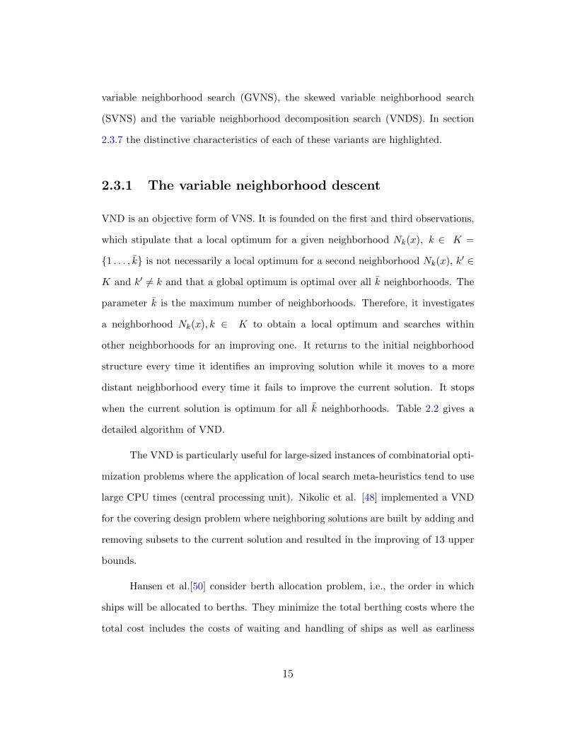
2.3.1 The variable neighborhood descent

VND is an objective form of VNS. It is founded on the first and third observations,

which stipulate that a local optimum for a given neighborhood Nk(x), k ∈ K =

{1 . . . , k} is not necessarily a local optimum for a second neighborhood Nk(x), k′ ∈

K and k′ 6= k and that a global optimum is optimal over all k neighborhoods. The

parameter k is the maximum number of neighborhoods. Therefore, it investigates

a neighborhood Nk(x), k ∈ K to obtain a local optimum and searches within

other neighborhoods for an improving one. It returns to the initial neighborhood

structure every time it identifies an improving solution while it moves to a more

distant neighborhood every time it fails to improve the current solution. It stops

when the current solution is optimum for all k neighborhoods. Table 2.2 gives a

detailed algorithm of VND.

The VND is particularly useful for large-sized instances of combinatorial opti-

mization problems where the application of local search meta-heuristics tend to use

large CPU times (central processing unit). Nikolic et al. [48] implemented a VND

for the covering design problem where neighboring solutions are built by adding and

removing subsets to the current solution and resulted in the improving of 13 upper

bounds.

Hansen et al.[50] consider berth allocation problem, i.e., the order in which

ships will be allocated to berths. They minimize the total berthing costs where the

total cost includes the costs of waiting and handling of ships as well as earliness

15

Table 2.2: Pseudo Code of the VND

1 Find an initial solution x ∈ X, set the best solution x∗=x, and k=1.

2 Do While (k ≤ k):

2.1 Find the best neighbor x′ ∈ Nk(x) of x

2.2 If f(x′) < f(x) then

set x = x′ and k = 1;

If f(x′) < f(x∗), set x∗ = x′

else

set k = k + 1.

or tardiness. They propose a VNS, and compare it to a multi-start heuristic, a

genetic algorithm, and a memetic algorithm. They show that the VNS is on average

the better of the three approaches. Qu et al. [57] apply the VND to the delay-

constrained least-cost multicast routing problem, which reduces to the NP-complete

delay-constrained Steiner Tree. They investigate the effect of the initial solution

by considering two initial solutions: one based on the shortest path and one on

bounded-delay, and consider three types of neighborhoods. They show that the

VND outperforms the best existing algorithms. Kratica et al. [35] use a VND

within large shaking neighborhoods to solve a balanced location problem. This

latter problem consists of choosing the location of p facilities while balancing the

number of clients assigned to each location. They show that their implementation

is very fast and reaches the optimal solution for small instances. For large instances

where the optimal solution value is unknown, the VNS outperforms a state-of-the-art

modified genetic algorithm.

16

2.3.2 The reduced variable neighborhood descent

The RVNS is a slightly different provision of the VNS; yet, it retains its basic

structure. It is based upon the third principle of the VNS which states that a

global optimum is the best solution a cross all possible neighborhoods. It is a

stochastic search. The outer loop constitutes the stopping. The inner loop conducts

a search over a fixed set of k nested neighborhoods N1(x) ⊂ N2(x) ⊂ . . . , ⊂ Nk(x)

that are centered on a randomly generated focal point x. A solution x′ ∈ X is

generated using a stochastic procedure Shake (x, k) which slightly perturbs the

solution x. For instance, in non-linear programming where the final solution of

any optimization solver depends on the solution it is fed, procedure Shake (x, k)

would alter the value of one or more of the variables of x by small amounts δ where

the altered variable(s) and δ are randomly chosen. Subsequently, either the focal

point of the search is changed to the current solution x or an enlarged neighborhood

search is to be undertaken. Specifically, when f(x′) < f(x), the inner loop centers

its future search space on the most reduced neighborhood around x′ (i.e., it sets

x=x′ and k=1). Otherwise, it enlarges its sampling space search by incrementing

k but maintains its current focal point x. Every iteration of the inner loop can

be assimilated to injecting a cut to the minimization problem, if each new bound

improves the existing one; thus, to fathoming a part of the search space.

Table 2.3 gives a detailed pseudo code of the RVNS. This approach is well

suited for multi-start VNS-based strategies where RVNS can be replicated with

different initial solutions x ∈ X and the best solution over all replications is retained.

It behaves like a Monte Carlo simulation except that its choices are systematic rather

than random. It is a more general case of Billiard simulation; a technique that was

applied to point scattering within a square.

17

Table 2.3: Pseudo Code of the RVNS

1 Find an initial solution x ∈ X; set the best solution x∗=x, and k=1.

2 Choose a stopping condition.

3 Do While (Stopping condition is False):

Do While (k ≤ k)

3.1 x′ ← Shake (x, k)

3.2 If f(x′) < f(x), then

set x=x′ and k=1;

If f(x′) < f(x∗) set x∗=x′

else

set k=k+1.

RVNS is particularly useful when the instances are large or when the local

search is expensive [53, 47]. Computational proof is given in section 2.3.4 for the

high school timetabling problem, where the performance of the RVNS is been to

better than be the GVNS, which applies simulated annealing as the local search [59].

Hansen et al. [53] further substantiated the claim regarding the speed of the RVNS.

They compare the performance of the RVNS to that of the fast interchange heuristic

for the p-median problem. They show that the speed ratio can be as large as 20

for comparable average solutions. For the same problem, Crainic et al. [72] provide

additional performance analysis of a parallel implementation of the RVNS. Maric et

al. [43] hybridize the RVNS with a standard VNS. They compare the performance of

the resulting heuristic to a swarm optimization algorithm and a simulated annealing

one for the bi-level facility location problem with clients’ preference, but unlimited

capacity for each facility. They show that the hybrid heuristic outperforms the other

two in large-scale instances and is competitive in the case of smaller instances.

18

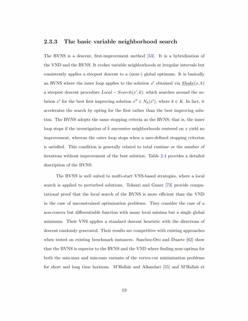
2.3.3 The basic variable neighborhood search

The BVNS is a descent, first-improvement method [53]. It is a hybridization of

the VND and the RVNS. It evokes variable neighborhoods at irregular intervals but

consistently applies a steepest descent to a (near-) global optimum. It is basically

an RVNS where the inner loop applies to the solution x′ obtained via Shake(x, k)

a steepest descent procedure Local − Search(x′, k), which searches around the so-

lution x′ for the best first improving solution x′′ ∈ Nk(x′), where k ∈ K. In fact, it

accelerates the search by opting for the first rather than the best improving solu-

tion. The BVNS adopts the same stopping criteria as the RVNS; that is, the inner

loop stops if the investigation of k successive neighborhoods centered on x yield no

improvement, whereas the outer loop stops when a user-defined stopping criterion

is satisfied. This condition is generally related to total runtime or the number of

iterations without improvement of the best solution. Table 2.4 provides a detailed

description of the BVNS.

The BVNS is well suited to multi-start VNS-based strategies, where a local

search is applied to perturbed solutions. Toksari and Guner [73] provide compu-

tational proof that the local search of the BVNS is more efficient than the VND

in the case of unconstrained optimization problems. They consider the case of a

non-convex but differentiable function with many local minima but a single global

minimum. Their VNS applies a standard descent heuristic with the directions of

descent randomly generated. Their results are competitive with existing approaches

when tested on existing benchmark instances. Sanchez-Oro and Duarte [62] show

that the BVNS is superior to the RVNS and the VND where finding near-optima for

both the min-max and min-sum variants of the vertex-cut minimization problems

for short and long time horizons. M’Hallah and Alkandari [55] and M’Hallah et

19

Table 2.4: Pseudo Code of the BVNS

1 Find an initial solution x ∈ X; set the best solution x∗=x, and k=1.

2 Choose a stopping condition.

3 Do While (Stopping condition is False):

Do While (k ≤ k)

3.1 x′ ← Shake(x, k).

3.2 x′′ ← Local − Search (x′, k).

3.3 If f(x′′) < f(x), then

set x = x′′ and k = 1;

If f(x′′) < f(x∗) set x∗ = x′′

else

set k = k + 1.

al. [56] apply BVNS for packing unit spheres into the smallest cube and sphere,

respectively, highlighting the utility of the local search.

2.3.4 The general variable neighborhood search

The GVNS is a low-level hybridization of the BVNS with the RVNS and the VND

[51, 52]). A detailed description of the GVNS is given in Table 2.5. First, it applies

the RVNS to obtain a feasible initial solution to the problem (step 2 in Table 2.5)

in lieu of directly sampling a feasible solution x ∈ X (as in step 1 in Table 2.4).

This is particularly useful in instances where finding a feasible solution is in itself

an NP-hard problem. Second, it replaces the local search (Step 3.2 in Table 2.4) of

the BVNS with a VND (Step 5.2 in Table 2.5). In addition, it samples the points x′

from the kth neighborhood Nk(x) of the current solution x. In fact, it uses procedure

20

Shake(x, k).

Table 2.5: Pseudo Code of the GVNS

1 Find an initial solution x.

2 x′ ← RV NS (x) starting with x to obtain a feasible solution x′ ∈ X .

3 Set the best solution x∗=x′ the current solution x=x′ and the neighbor-hood counter k=1.

4 Choose a stopping condition.

5 Do While (Stopping condition is False)

Do While (k ≤ k):

5.1 x′ ← Shake (x, k) .

5.2 x′′ ← V ND (x′).

5.3 If f(x′′) < f(x) , then

set x=x′′ and k=1;

If f(x′′) < f(x∗) set x∗=x′′

else

set k=k+1.

GVNS was applied to large-sized vehicle routing problems with time win-

dows [64, 46] and to the traveling salesman problem [46]. The implementation of

Mladenovic et al. [46] provides the best upper bounds in more than half of the

existing benchmark instances. It was particularly useful because identifying initial

feasible solutions and maintaining feasibility during the shaking procedure and the

neighborhood investigation was a challenging task.

21

2.3.5 The skewed variable neighborhood search

The SVNS is a modified BVNS where a non-improving solution x′′ may become the

new focal point of the search, when this solution x′′ is far enough from the current

one x, but its value f(x′′) is not much worse than f(x), the value of the current

solution x [27]. The SVNS is motivated by the topology of search spaces. The

search gets trapped in a local optimum and cannot leave it because all neighboring

solutions are worse. Yet, if it opts for a “not-too-close” neighborhood, it may reach

the global optimum. This neighborhood should not be too far and the neighbor

should not be too much worse can to enable to return to the current neighborhood,

if the exploration fails to identify an improving solution.

Table 2.6: Pseudo Code of the SVNS

1 Find an initial solution x ∈ X; set the best solution x∗=x, and k=1.

2 Choose a stopping condition.

3 Do While (Stopping condition is False)

Do While (k ≤ k):

3.1 x′ ← Shake (x, k).

3.2 x′′ ← Local − Search (x′, k).

3.3 If f(x′′)− αρ(x, x′′) < f(x), then

set x=x′′ and k=1;

If f(x′′) < f(x∗) set x∗=x′′

else

set k=k+1.

The difference between x and x′′, is measured in terms of a distance ρ(x, x′′) while

the difference between f(x′′) and f(x) is considered tolerable if it is less than an

22

expression pondering the distance ρ(x, x′′) by a parameter α. That is, the condition

f(x′′) < f(x) of step 3.3 in Table 2.4 is replaced by f(x′′) − αρ(x, x′′) < f(x). A

detailed description of the BVNS is provided in Table 2.6.

The utility of the SVNS is demonstrated by Hansen and Mladenovic [27] for

the weighted maximum satisfiability of logic problem for which the SVNS performs

better than the GRASP (Greedy Randomized Adaptive Search Procedure) and Tabu

Search, for medium and large problems, respectively. The choice of α is generally

based on an analysis of the behavior of a multiple start VNS.

2.3.6 The variable neighborhood decomposition search

The VNDS is used in the particular case, where the set X of feasible solutions is

finite. Yet, its extension to the infinite case is possible. It is one of two techniques

designed to reduce the computational time of local search algorithms. Even though

they investigate a single neighborhood structure, local search heuristics tend to have

their runtime increase significantly as the size of the combinatorial problems become

large [53]. It is “a BVNS within successive approximations decomposition” scheme

[53]. That is, both the VNDS and the BVNS have the same algorithmic steps

except that procedures Shake and Local−Search of steps 3.1 and 3.2 of Table 2.4,

respectively, are implemented on a partial solution y of free variables, whereas all

other variables remain fixed as in x throughout the random selection of x′ ∈ X and

the local search for an improving solution x′′ ∈ X. A detailed description of the

pseudo-code of the VNDS is given in Table 2.7.

Obtaining a random solution x′ ∈ X from the current solution x ∈ X via

procedure Shake(x, k, y) entails choosing values for the partial solution y, which

consists of a set of free variables of x, while ensuring that the new value of every

23

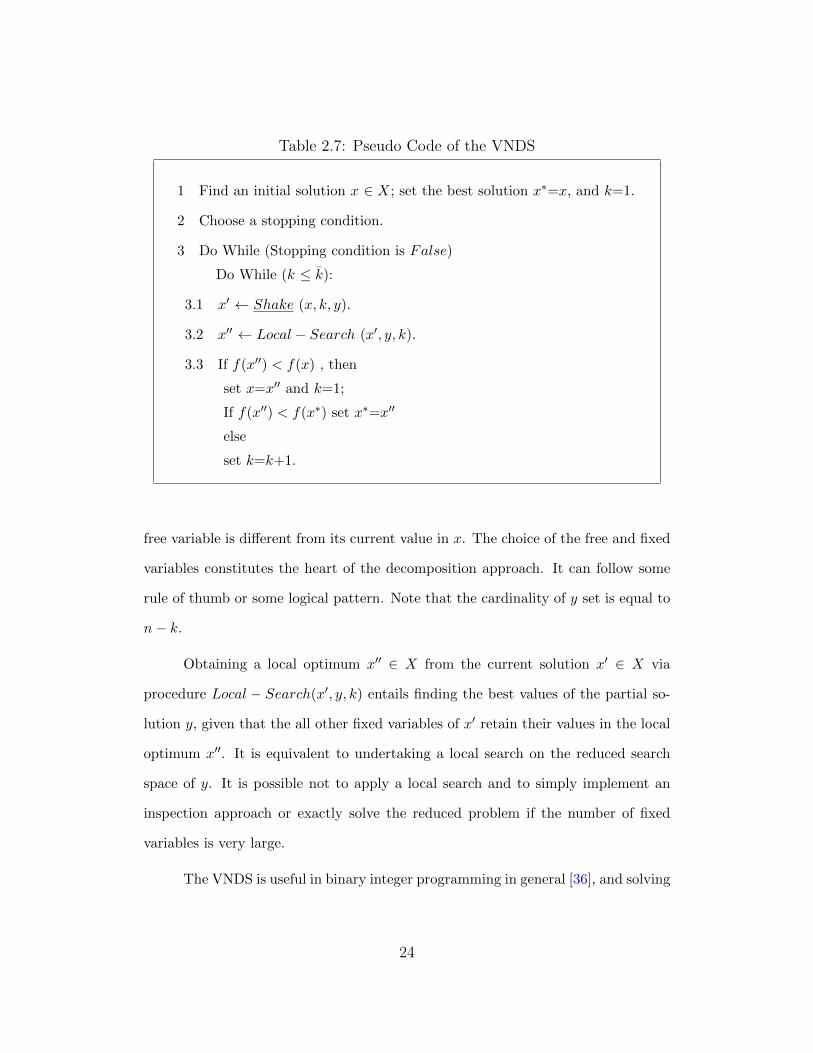
Table 2.7: Pseudo Code of the VNDS

1 Find an initial solution x ∈ X; set the best solution x∗=x, and k=1.

2 Choose a stopping condition.

3 Do While (Stopping condition is False)

Do While (k ≤ k):

3.1 x′ ← Shake (x, k, y).

3.2 x′′ ← Local − Search (x′, y, k).

3.3 If f(x′′) < f(x) , then

set x=x′′ and k=1;

If f(x′′) < f(x∗) set x∗=x′′

else

set k=k+1.

free variable is different from its current value in x. The choice of the free and fixed

variables constitutes the heart of the decomposition approach. It can follow some

rule of thumb or some logical pattern. Note that the cardinality of y set is equal to

n− k.

Obtaining a local optimum x′′ ∈ X from the current solution x′ ∈ X via

procedure Local − Search(x′, y, k) entails finding the best values of the partial so-

lution y, given that the all other fixed variables of x′ retain their values in the local

optimum x′′. It is equivalent to undertaking a local search on the reduced search

space of y. It is possible not to apply a local search and to simply implement an

inspection approach or exactly solve the reduced problem if the number of fixed

variables is very large.

The VNDS is useful in binary integer programming in general [36], and solving

24

large-scale p-median problems [53] in particular. The p-median problem involves

choosing the location of p facilities among m potential ones in order to satisfy the

demand of a set of users at least cost. Lazic et al. [36] provide computational proof

that the VNDS performs best on all performance measures of solution approaches

including computation time, optimality gap, and solution quality. Hanafi et al. [60]

tackle the 0-1 mixed-integer programming problem using a special VNDS variant.

This latter exploits the information obtained from an iterative relaxation-based

heuristic in its search. This information serves to reduce the search space and avoid

the reassessment of the same solution during different replications of the VNDS.

The heuristic adds pseudo-cuts based on the objective function value to the original

problem to improve the lower and upper bounds; thus, it reducing the optimality

gaps. The approach yields the best average optimality gap and running time for

binary multi-dimensional knapsack benchmark instances. It is inferred that the

approach can yield tight lower bounds for large instances.

2.3.7 Comparison of the VNS variants

The VNS was designed for combinatorial problems, but is applicable to any global

optimization problem. It explores distant neighborhoods of incumbent solutions in

search for global optima. It is simple and requires very few parameters. The main

characteristics of its seven variants are summarized in Table 2.8. The VNS has been

hybridized at different levels with other heuristics and meta-heuristics. For instance,

Kandavanam et al. [20] consider route multi-class network communication planning

problem in order to satisfy service quality. They hybridize the VNS with a genetic

algorithm and apply the hybrid heuristic to maximizing the residual bandwidth of

all links in the network, while meeting the requirements of the expected quality of

service.

25

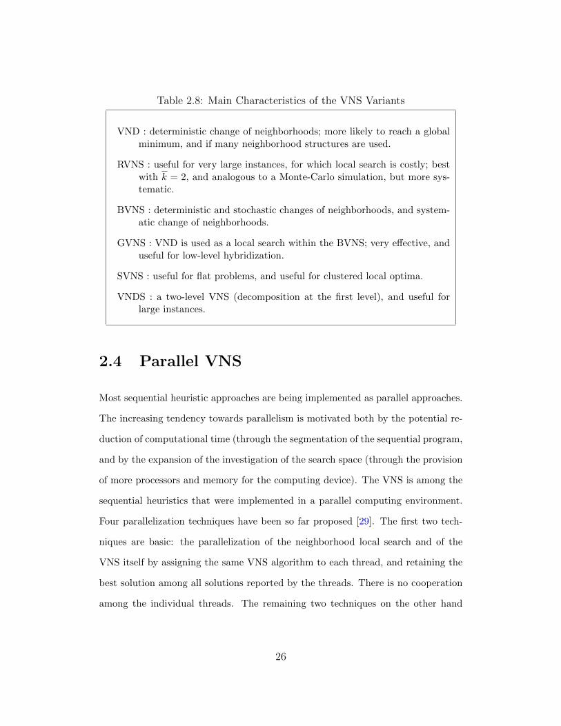
Table 2.8: Main Characteristics of the VNS Variants

VND : deterministic change of neighborhoods; more likely to reach a globalminimum, and if many neighborhood structures are used.

RVNS : useful for very large instances, for which local search is costly; bestwith k = 2, and analogous to a Monte-Carlo simulation, but more sys-tematic.

BVNS : deterministic and stochastic changes of neighborhoods, and system-atic change of neighborhoods.

GVNS : VND is used as a local search within the BVNS; very effective, anduseful for low-level hybridization.

SVNS : useful for flat problems, and useful for clustered local optima.

VNDS : a two-level VNS (decomposition at the first level), and useful forlarge instances.

2.4 Parallel VNS

Most sequential heuristic approaches are being implemented as parallel approaches.

The increasing tendency towards parallelism is motivated both by the potential re-

duction of computational time (through the segmentation of the sequential program,

and by the expansion of the investigation of the search space (through the provision

of more processors and memory for the computing device). The VNS is among the

sequential heuristics that were implemented in a parallel computing environment.

Four parallelization techniques have been so far proposed [29]. The first two tech-

niques are basic: the parallelization of the neighborhood local search and of the

VNS itself by assigning the same VNS algorithm to each thread, and retaining the

best solution among all solutions reported by the threads. There is no cooperation

among the individual threads. The remaining two techniques on the other hand

26

utilize cooperation mechanisms to upgrade the performance level of the algorithm.

They are more complex and involve intricate parallelization [39, 72] to synchronize

communication. A detailed description of these four techniques follows.

The first parallelization technique is the synchronous parallel VNS (SPVNS).

It is the most primary parallelization technique [39]. It is designed to shorten the

Table 2.9: Pseudo Code of the SPVNS

1 Find an initial solution x ∈ X; set the best solution x∗=x, and k=1.

2 Choose a stopping condition.

3 Do While (Stopping condition is False) Do While (k ≤ k):

3.1 x′ ← Shake (x).

3.2 Divide the neighborhood Nk(x′) into np subsets.

3.3 For every processor p, p=1. . . ,np, x′′p ← Local − Search (x′, k).

3.4 Set x′′ such that f(x′′) = maxp=1,np

{f(x′′p)}

3.5 If f(x′′) < f(x), then

set x=x′′ and k=1;

If f(x′′) < f(x∗) set x∗=x′′

else

set k=k+1.

runtime through the parallelization of the local search of the sequential VNS. In

fact, the local search is the most time-demanding part of the algorithm. The SPVNS

splits the neighborhood into np parts and assigns each subset of the neighborhood

to an independent processor, which returns to the master processor an improving

neighbor within its subset of the search space. The master processor sets the best

among the np neighbors returned by the np processors as the current solution. Table

27

2.9 provides the pseudo code of the SPVNS, adapted from Garcia et al. [39].

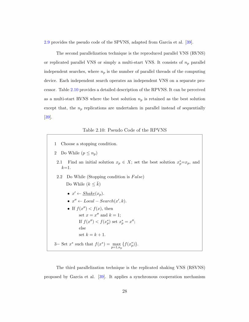
The second parallelization technique is the reproduced parallel VNS (RVNS)

or replicated parallel VNS or simply a multi-start VNS. It consists of np parallel

independent searches, where np is the number of parallel threads of the computing

device. Each independent search operates an independent VNS on a separate pro-

cessor. Table 2.10 provides a detailed description of the RPVNS. It can be perceived

as a multi-start RVNS where the best solution np is retained as the best solution

except that, the np replications are undertaken in parallel instead of sequentially

[39].

Table 2.10: Pseudo Code of the RPVNS

1 Choose a stopping condition.

2 Do While (p ≤ np)

2.1 Find an initial solution xp ∈ X; set the best solution x∗p=xp, andk=1.

2.2 Do While (Stopping condition is False)

Do While (k ≤ k)

• x′ ← Shake(xp).

• x′′ ← Local − Search(x′, k).

• If f(x′′) < f(x), then

set x = x′′ and k = 1;

If f(x′′) < f(x∗p) set x∗p = x′′;

else

set k = k + 1.

3− Set x∗ such that f(x∗) = maxp=1,np

{f(x∗p)}.

The third parallelization technique is the replicated shaking VNS (RSVNS)

proposed by Garcia et al. [39]. It applies a synchronous cooperation mechanism

28

through a conventional master-slave methodology. The master processor operates

a sequential VNS, and sends its best incumbent to every slave processor, which

shakes this solution to obtain a starting point for its own local search. In turn, each

slave returns its best solution to the master. This latter compares all the solutions

obtained by the slaves, retains the best one and subjects it to its sequential VNS.

This information exchange is repeated until a stopping criterion is satisfied. The

Table 2.11: Pseudo Code of the RSVNS

1 Find an initial solution x ∈ X; set the best solution x∗=x, and k=1.

2 Choose a stopping condition.

3 Do While (Stopping condition is False)

Do While (k ≤ k)

3.1 For p=1. . . ,np

• Set xp=x

• x′ ← Shake (x′p).

• x′′p ← Local − Search (x′p, k).

3.2 Set x′′ such that f(x′′) = maxp=1,np

{f(x′′p)}

3.3 If f(x′′) < f(x), then

set x=x′′ and k=1;

If f(x′′) < f(x∗p) set x∗p=x′′;

else

set k=k+1.

fact that VNS permits changing neighborhoods and types of local search makes

this type of parallelization possible. Different neighborhoods or local searches can

be performed by independent processors and the resulting information is channeled

to the master processor which analyzes its results to obtain the best solution and

29

conveys it to the other slaves. Maintaining a trace of the last step undertaken by

every processor strengthens the search as it avoids the duplication of computational

efforts. Table 2.11 provides a detailed description of the RSVNS. It can be perceived

as a VNS with a multi-start shaking and local search where the best local solution

among np ones is retained as the best local solution and routed to each of the np

processors [39]. A comparison of the performance of these first three parallel VNS

algorithms is undertaken by Garcia et al. [39] for the p-median problem.

The fourth and last parallelization technique is the cooperative neighborhood

VNS (CNVNS) suggested by Crainic et al. [72] and Moreno-Perez et al. [38]. It

is particularly suited to combinatorial problems such as the p-median problem. It

deploys a cooperative multi-search strategy to the VNS while exploring a central-

memory mechanism. It coordinates many independent VNSs by asynchronously

exchanging the best incumbent obtained so far by all processors. Its implementation

preserves the simplicity of the original sequential VNS ideas. Yet, its asynchronous

cooperative multi-search offers a broader exploration of the search space thanks

to the different VNSs being applied by the different processors. Each processor

undertakes an RVNS, and communicates with a central memory or the master,

every time it improves the best global solution. In turn, the master relays this

information to all other processors so that they update their knowledge about the

best current solution. That is, no information is exchanged in terms of the VNS

itself. The master is responsible for launching and stopping the parallel VNS. In

case of Crainic et al. [72], the parallel algorithm is an RVNS where the local search

is omitted; resulting in a faster algorithm. Table 2.12 and Table 2.13 gives a detailed

description of the CNVNS as originally intended and as described by Moreno-Perez

et al. [38]. A comparison of the performance of the four parallel VNS algorithms is

undertaken by Moreno-Perez et al. [38] for the p-median problem.

30

Table 2.12: Pseudo Code of the CNVNS: Master’s Algorithm

1 Find an initial solution x ∈ X; set the best solution x∗ = x, and kp=1,p = 1, . . . , np

2 Choose a stopping condition.

3 Set xp = x

4 For p = 1, . . . , np , launch RVNS with xp as its initial solution.

5 When processor p′ sends x′′p′ .

5.1 If f(x′′p′) < f(x), then update current best solution setting x = x′′p′and send it to all np processors.

6 When processor p′ requests best current solution, send x

Table 2.13: Pseudo Code of the CNVNS: Slave’s Algorithm

1 Obtain initial solution xp from master; set the best solution x∗p = xp,and randomly choose k ∈ {1, . . . , k}

2 Do While (k ≤ k)

2.1 x′ ← Shake (x).

2.2 If f(x′p) < f(xp), then

set xp = x′p and k=1;

if f(x′p) < f(x∗p) set x∗p = xp.

else

send x∗p to the master;

receive xp from master;

set k=k+1.

31

2.5 Discussion and conclusion

The VNS is a general framework for solving optimization problems. Its success-

ful application to different continuous and discrete problems is advocating for its

wider use to non-traditional areas such as neural networks and artificial intelligence.

The VNS owes its success to its simplicity and to its limited number of parame-

ters:the stopping criterion and maximal number of neighborhoods. Depending on

the specific problem at hand, a VNS variant may be deemed more appropriate than

other variants. In fact, a judicious choice of the neighborhood structure and local

search strategy could determine the success of an approach. The local search may

vary from exact optimization techniques for relaxed or reduced problems to gradi-

ent descent, line search, steepest descent, to meta-heuristics like Tabu Search and

simulated annealing.

32

Chapter 3

Packing Unit Spheres into the

Smallest Sphere Using the VNS

and NLP

3.1 Introduction

Sphere packing problems (SPP) consist comprise of packing spheres into a sphere of

the smallest possible radius. It has many important real-life applications including

materials science, radio surgical treatment, communication, and other vital fields.

In materials science, random sphere packing is a model to represent the structure

of liquids, proteins, and glassy materials. The model is used to study phenomena

such as electrical conductivity, fluid flow, stress distribution and other mechanical

properties of granular media, living cells, random media chemistry and physics. SPP

also entails the investigation of processes such as sedimentation, compaction, and

sintering [76]. In radio surgical treatment planning, sphere packing is crucial to

33

X-ray tomography. In [75] a problem on how to pack minimum number of unequal

spheres into a three dimensions bounded region, in connection with radio-surgical

treatment planning, is studied. It is used for treating brain and sinus tumor (see

Figure 3.1).

Figure 3.1: X-Ray

During the operation, medical unit should not effect other organs. Gamma

knife is one of more effective radio-surgical modalities. It can be described as ra-

dioactive dosage treatment planning. A high radiation dose is called the shot which

can be viewed as a sphere. These shots are ideal equal spheres to be packed into a

container, but also they could be of different spheres. The tumor can be viewed as an

approximate spherical container. No shots are allowed outside the container, which

means that the radiation shots are only hitting the tumor cells and not the healthy

ones. Multiple shots are usually applied at various locations and may touch the

boundary of the target. They avoid overlapping and touch each other. The stronger

the high packing density, the more doses delivered. The target of the search to

minimize the number of shots into the container (The tumor). As a result, this ap-

34

proach has met with certain success in medical applications. Dynamic programming

algorithm is being used to find the optimum number of shots.

In digital communication and storage, it emerges in compact disks, cell phones,

and the Internet [15, 74]. The most frequent application of minimum sphere pack-

ing problem is connected with location of antennas. For example it is crucial in

antenna location in some large warehouse or container yards (see Figure 3.2). Each

article usually has radio frequency identifier (RFID) or tag. The management of the

warehouse wants to locate minimum number of antennas that cover all warehouse

such that vehicles, connected with the antenna system, are able to find any article.

The radii of each antenna are known in advance. This system provides real-time

location visibility, illuminating vital information that is needed [6].

Figure 3.2: Warehouse

Other applications of sphere packing are encountered in powder metallurgy

for three-dimensional laser cutting [42]; cutting different natural crystals; layout of

computers, buildings, etc.

In this chapter the special case of packing unit spheres into the smallest

sphere (PSS) is considered. PSS entails packing n identical spheres, of radius 1

35

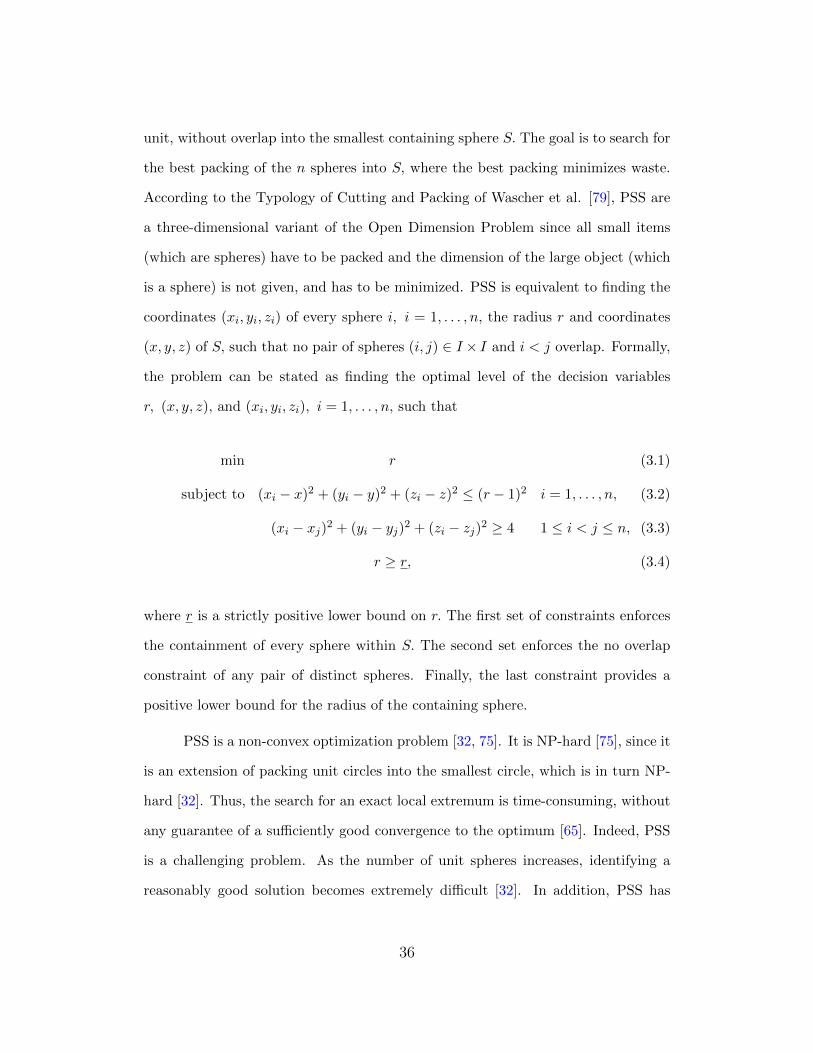
unit, without overlap into the smallest containing sphere S. The goal is to search for

the best packing of the n spheres into S, where the best packing minimizes waste.

According to the Typology of Cutting and Packing of Wascher et al. [79], PSS are

a three-dimensional variant of the Open Dimension Problem since all small items

(which are spheres) have to be packed and the dimension of the large object (which

is a sphere) is not given, and has to be minimized. PSS is equivalent to finding the

coordinates (xi, yi, zi) of every sphere i, i = 1, . . . , n, the radius r and coordinates

(x, y, z) of S, such that no pair of spheres (i, j) ∈ I × I and i < j overlap. Formally,

the problem can be stated as finding the optimal level of the decision variables

r, (x, y, z), and (xi, yi, zi), i = 1, . . . , n, such that

min r (3.1)

subject to (xi − x)2 + (yi − y)2 + (zi − z)2 ≤ (r − 1)2 i = 1, . . . , n, (3.2)

(xi − xj)2 + (yi − yj)2 + (zi − zj)2 ≥ 4 1 ≤ i < j ≤ n, (3.3)

r ≥ r, (3.4)

where r is a strictly positive lower bound on r. The first set of constraints enforces

the containment of every sphere within S. The second set enforces the no overlap

constraint of any pair of distinct spheres. Finally, the last constraint provides a

positive lower bound for the radius of the containing sphere.

PSS is a non-convex optimization problem [32, 75]. It is NP-hard [75], since it

is an extension of packing unit circles into the smallest circle, which is in turn NP-

hard [32]. Thus, the search for an exact local extremum is time-consuming, without

any guarantee of a sufficiently good convergence to the optimum [65]. Indeed, PSS

is a challenging problem. As the number of unit spheres increases, identifying a

reasonably good solution becomes extremely difficult [32]. In addition, PSS has

36

an infinite number of solutions with identical minimal radii. In fact, any solution

may be rotated or reflected or may have free spheres which can be slightly moved

without enlarging the radius of the containing sphere. Finally, there is the issue of

computational accuracy and precision.

Solving PSS via an off-the-shelf non-linear programming (NLP) solver is gen-

erally not successful. In fact, most of these solvers fail to identify global optima

because of PSS’ difficulty, which gets further amplified as the problem size increases

(since the number of local minima increases too). Subsequently, PSS should be

solved by a mixture of search heuristics with local exhaustive (exact) search of local

minima or their approximations as suggested in [67, 32]. This chapter follows this

line of research. It tackles PSS using a hybrid heuristic which combines these two

main components. It applies a variable neighborhood search (VNS) which investi-

gates different neighborhoods of the incumbent solution, and a special purpose NLP

solver to locally search for one or more minima within each neighborhood.

Section 3.2 reviews the most prominent literature in the area of sphere pack-

ing. Section 3.3 details the proposed approach. Section 3.4 investigates its per-

formance. Specifically, this section demonstrates the superiority of the proposed

approach in terms of accuracy and precision, provides new upper bounds for 14

instances, and determines the utility of VNS and the local search. Finally, section

3.5 is a summary.

3.2 Literature review

Sphere packing is considered when the container three-dimensional into which the

sphere are to be packed is a cube, a parallelepiped, a cylinder, a polytope, or a

sphere.

37

Gensane [22] adapts the Billiard simulation to the problem of identifying

the largest radius of n identical spheres that fit inside a unitary cube. Billiard

simulation is a stochastic method that mimics the idealized movement of billiard

balls inside a domain, with the initial centers of the balls and their directions being

randomly fixed. The resulting configuration emanates from probabilistic choices. To

improve the convergence of the stochastic algorithm, different types of local searches

were considered. These included moving the spheres randomly in a random walk

simulation, decreasing the magnitude of the stochastic movements as the size of the

spheres increased, and perturbing all spheres simultaneously.

Stoyan and Yaskov [66] focus on finding the minimal height of a paral-

lelepiped (L,W,H) that packs n identical spheres. They model the problem

as a NLP with a linear objective function and linear and quadratic constraints.

They approximately solve the model using a special search tree in conjunction with

a modification of the Zoutendijk method [80] of feasible directions to calculate local

minima, and a modification of the decremental neighborhood method to search for

an approximation to the global minimum.

Using the same technique, Stoyan and Yaskov [68] tackle the problem of min-

imizing the height H of a right circular cylinder, of known radius r, that packs n

identical spheres. The authors obtain the best results to date for n = 498, 499,

and 500. Their approach is very effective for n ≤ 500, and can handle instances for

n ≤ 2000.

Stoyan et al. [77] use techniques similar to those considered in [67] to identify a

packing of n non-identical spheres, each of radius ri, i ∈ I, into a parallelepiped

of fixed length L and width W but of variable height H with the objective of

minimizing H. The authors provide numerical results with up to 60 spheres.

38

Yaskov et al. [21] tackle the problem of maximizing the number of identical

spheres that can be packed into a cylindrical composed domain. They construct a

mathematical model based on the concept of Φ-functions [78], and design a solution

algorithm based on a modification of the optimization method by groups of variables.

Wang [75] formulates mathematically the automated radio surgical treatment

planning problem as the packing of spheres into a three-dimensional region with a

packing density greater than a given threshold level. He proves that this packing

problem is NP-complete and proposes an approximate algorithm to solve it.

Sutou and Dai [70] assimilate the automated radio surgical treatment plan-

ning problem to packing non-identical spheres in a three-dimensional polytope with

the objective of maximizing the volume of the packed spheres. They formulate

the problem as a non-convex optimization one with quadratic constraints and a

linear objective function. They propose a variety of algorithms which outperform

the generic algorithm for the general non-convex quadratic program. In fact, they

incorporate heuristics into the generic algorithm to strengthen its efficiency. They

demonstrate its efficiency computationally for limited problem sizes.

Stoyan and Yaskov [69] consider the problem of packing the maximal number

of congruent hyper spheres of unit radius into a larger hyper sphere of given radius.

They construct a mathematical model, and approximately resolve it by solving a

sequence of packing subproblems –whose objective functions are linear– using the

Zoutendijk feasible direction method. Starting points are generated in accordance

with the lattice packing of hyperspheres translated on various vectors or in a random

way. They improve the convergence of their sequential approach by perturbing the

lattice packing.

Hales [24] proves the Kepler conjecture which stipulates that the packing

39

density of identical three-dimensional spheres cannot exceed π√18. Bezdek [11] brings

forth a strong Kepler conjecture which alleges that the density of at least two equal

spheres in a sphere of the three-dimensional space of constant curvature is less than

π√18.

Birgin and Sobral [13] propose a reduced model for PSS. They aggregate the

n(n−1)2 non-overlap constraints into a single constraint:

n−1∑i=1

n∑j=i+1

max{0, 4− (xi − xj)2 − (yi − yj)2 − (zi − zj)2} = 0, (3.5)

and implement a reduction approach that avoids computing many of the n(n−1)2

terms of the sum. In fact, only terms relative to spheres that could potentially be

touching are included. They solve the resulting model, starting from several initial

solutions, using a local solver that is based on an augmented Lagrangian method

for smooth general constrained minimization. They report solutions for instances

with up to 100 spheres.

Liu et al. [37] adopt an unconstrained model for the problem where they ag-

gregate all the constraints of PSS and “Lagrange” them into the objective function:

min r +n∑i=1

d2i0 +

n−1∑i=1

n∑j=i+1

d2ij , (3.6)

where d2ij = max{0, 4− (xi − xj)2 − (yi − yj)2 − (zi − zj)2}, (3.7)

and d2i0 = max{0, (xi − x)2 + (yi − y)2 + (zi − z)2 − (r − 1)2}. (3.8)

Their model is inspired from quasi physics where spheres that are in contact

have extrusive elastic energy, and a system is in equilibrium when all elastic energies

are nil. They solve the resulting model using a heuristic which combines the energy

landscape paving (ELP) method with an adaptive step length gradient descent pro-

40

cedure. ELP is an optimization strategy that mimics the Monte Carlo simulation

while using concepts from simulated annealing.

Pfoertner [1] posts the best known radii r∗i of n identical spheres that can be

packed into a containing sphere of radius one. This problem can be stated as: equal

sphere packing (EPP)

max ri (3.9)

Subject to (xi − x)2 + (yi − y)2 + (zi − z)2 ≤ (1− ri)2 i = 1, . . . , n, (3.10)

(xi − xj)2 + (yi − yj)2 + (zi − zj)2 ≥ 4r2i 1 ≤ i < j ≤ n,(3.11)

0 ≤ ri ≤ 1 i = 1, . . . , n. (3.12)

The EPP model is equivalent model to the PSS model. In fact, its solution value r∗i

can be mathematically mapped to the PSS optimal solution value r∗ :

r∗ = 1r∗i. (3.13)

3.3 Proposed approach

PSS is a difficult problem. It has an infinite number of alternative optima, an expo-

nential number of local optima which are not globally optimal, and an uncountable

set of stationary points – i.e., solutions that satisfy the Karush Kuhn Tucker (KKT)

conditions but which do not correspond to local optima. Moreover, the solution

to a PSS problem is sensitive to the choice of the initial solution (as is the case of

non-linear optimization). Finally, the larger the number of spheres to be packed,

the larger the number of local minima and stationary points. Thus, the simple

multi-start global optimization strategies need more local minimizations to reach a

41

global minima [13].

PSS is herein solved using an approach that applies Schittkowski local search

(LS) as the intensification strategy and variable neighborhood search (VNS) as the

diversification strategy. In sections 3.3.1 and 3.3.2, detail LS and VNS, respectively,

are detailed.

3.3.1 Schittkowski’s local search

An approximate solution to PSS can be obtained using an off-the-shelf NLP solver.

However, its quality (i.e., its deviation from the optimal radius) depends both on

the initial solution fed to the solver and on its proximity to the global optimum. In

addition, there is no guarantee that the obtained solution is a local optimum. In

fact, the solution can be a saddle point. Moreover, the solver can stop for various

reasons such as no improving search direction, errors in evaluating function and

gradient values, violation of regularity conditions, etc.

To overcome the shortcomings of NLP solvers, a PSS problem is approxi-

mately solved via a better adapted NLP solver. It applies a NonLinear Program-

ming with Non-Monotone and Distributed Line Search (NLPQLP), the sequential

quadratic programming (SQP) algorithm to a non-monotone line search of Schit-

tkowski [63]. NLPQLP is designed to resolve smooth NLP problems. When the

solver aborts because of computational errors caused by inaccurate function or gra-

dient evaluations, a non-monotone line search is activated. Internal restarts are

performed in case of errors when computing the search direction due to inaccurate

derivatives. Additional automated initial and periodic scaling with restarts is imple-

mented. Schittkowski [63] reports that the extensive computational investigation of

the code on benchmark instances clearly demonstrated the improvements brought

42

up by the non-monotone search. He further indicates that more than 90 % of the

306 tested instances, were successfully solved, subject to a stopping tolerance of

10−7.

NLPQLP requires an initial solution and bounds for the variables of the prob-

lem. Providing loose bounds on the variables may hinder the convergence of the

solver to a feasible direction or induce computational errors. The radius r can be

bounded in two ways. A straightforward lower bound r assumes that the spheres

are not solid, and that S contains no unused volume. Subsequently, the minimal

volume of S is the sum of the volumes of the n spheres. It follows that the radius

of this utopian sphere is r = 3√n. A tighter lower bound uses the Kepler conjecture

[24] that the density of the best packing of n ≥ 2 non-overlapping spheres cannot

exceed π√18. Consequently, r = 3

√π√18n.

The upper bound r is estimated by assuming that the spheres can be fitted

into a cube of side c = 2d 3√ne, where dae is a integer such that dae − 1 < a ≤ dae.

The sphere fitting this cube has a radius r =√

3( c2)2.

From a mathematical point of view, having S centered at (0, 0, 0) or (r, r, r)

yield equivalent configurations since they can be obtained from each other via a sim-

ple transformation. However, LS did not handle negative values of the coordinates

will and often failed to converge to a feasible solution in the former case. Thus, each

of the coordinates (xi, yi, zi) of a small sphere i, i = 1, . . . , n, are bounded by 1 and

2r− 1. Similarly, these bounds apply to the coordinates (x, y, z) of the containing

sphere S. Tighter bounds can be used, but in many instances it let to infeasible

solutions. Our experimental investigation further indicated that most NLP solvers

(including LS) face difficulties in restoring containment feasibility if the initial r fed

to the solver is too small (even in the absence of overlap). Very loose bounds are

counter-productive too. They cause the local search to converge to local optima

43

that are too far from the global optimum.

It is believed that feeding the solver with a feasible initial solution speeds up

the search process and provides a better estimate for the global minima. Meanwhile

many newer NLP approaches claim their robustness with respect to the initial so-

lution and its feasibility. Herein, LS is started from both a feasible solution and

randomly generated solutions.

When started from an initial feasible solution, the search is denoted SLS.

The feasible solution is obtained using a very simple constructive heuristic which

packs the spheres in layers in a cube of side c. It positions sphere i, i = 1, . . . , n, in

(xi, yi, zi), where xi = 2d+1, yi = 2b+1, zi = 2a+1, with a, b, d integers satisfying

i = ac2 +bc+d. This heuristic is obviously very simple and does not yield a compact

packing of the spheres. On the other hand, it is very fast, causes no truncation or

roundoff errors, offers the spheres enough degrees of freedom to move, and gives LS

a feasible descent direction. Evidently, the lattice configuration is another feasible

configuration. However, it was discarded since it is suspected to correspond to the

optimal packing in many instances and represents a local minima for the others.

Thus, it may hinder the search for better quality optima.

When started with a random initial solution (which is not necessarily fea-

sible), the search is denoted as RLS. The random configuration is generated by

arbitrarily selecting the coordinates (x, y, z) and (xi, yi, zi), i = 1, . . . , n, from the

uniform[1, 2r − 1], and setting r = r. When RLS is restarted kM times, the search

is denoted as M-RLS (for Multistar RLS).

44

3.3.2 Variable neighborhood search

VNS is a metaheuristic which exploits systematically the idea of neighborhood

change, both in descent to local minima and in escape from the valleys which con-

tain them [27, 26, 28, 54, 45]. Its success emanates from three main characteristics.

First, a local minimum with respect to one neighborhood is not necessarily a local

minimum for another neighborhood. Second, a global minimum must be a local

minimum with respect to all possible neighborhood structures. Third, in many

problems including PSS, local minima with respect to one or more neighborhoods

are relatively close to each other.

In VNS the search is initiated with a feasible solution u for PSS with a radius

ru. It sets k = 1, and randomly generates a solution u′ from a neighborhood Nk(u)

of u. It then applies a local search to u′ (SLS or RLS depending on whether u′ is

feasible or not) to identify a local minimum u” ∈ Nk(u). If ru” improves the current

solution, the best solution is updated, i.e, the current solution u is set to u”. That

is, if ru” < ru∗ , then ru∗ is reset to ru”, and u∗ to u”. Differently stated, the focus

of the search is re-centered on u”. Consequently, k is reset to 1 and the search is

restarted by generating a random solution from the neighborhood N1(u). On the

other hand, if u” does not improve the current solution ru, a different neighborhood

of u is investigated. Specifically, k is incremented, and a different random solution

u′ from the new neighborhood Nk(u) of u is obtained, and the local search is applied

to u′ to get u”. It represents the inner loop of the method. When it is completed,

then k is set to 1 and the inner loop is started again. It is repeated until the VNS

runtime is smaller than the maximum runtime allowed. The detailed algorithm of

VNS is given in Algorithm 1.

A solution u′ from a neighborhood Nk(u), k = 1, . . . , k, of u is generated

45

Algorithm 1 Detailed Algorithm of the VNS for PSS

Input

1 An initial feasible solution u = (xi, yi, zi)i=1,...,n, and ru the correspondingradius of S.

2 t, the maximum runtime for VNS.

3 k, the maximum number of neighborhoods.

Output

1 An approximate optimal solution u∗ = (x∗i , y∗i , z∗i )i=1,...,n, and its associated

radius ru∗ .

Algorithm

1 Set u∗ = u and ru∗ = ru.

2 Do while t ≤ T

2.1 Set the neighborhood type k = 1.

2.2 Do while k ≤ k

2.2.1 Apply the procedure Shake(k,u,u′) to obtain a random solution u′ ∈Nk(u), where Nk(u) is the kth neighborhood of u.

2.2.2 Apply the local search with u′ as the starting solution, to get the newsolution u” and its associated value ru”.

2.2.3 If ru” < ru∗ , set k = 1, u∗ = u”, ru∗ = ru, and u = u”; else, set k = k+1.

using procedure Shake(k,u,u′). Let S[k] denote the kth closest sphere to the center

of the containing sphere S, and d[k] the distance that separates the centers of S[k]

and S. For k ≤ n, procedure Shake(k,u,u′) translates sphere S[k] by δx[k], δy[k] and δz[k]

in the x, y and z directions, respectively. The translation distances are randomly

generated from the Uniform[−∆,∆], where ∆ is the neighborhood parameter. If this

translation results in the violation of the lower (resp. upper) bound of a variable,

this latter is reset to its lower (resp. upper) bound. For n < k ≤ 2n, procedure

46

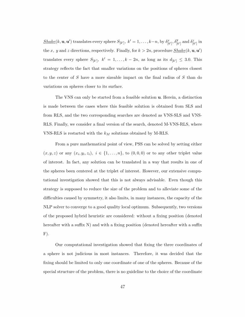
Shake(k,u,u′) translates every sphere S[k′], k′ = 1, . . . , k−n, by δx[k′], δ

y[k′] and δz[k′] in

the x, y and z directions, respectively. Finally, for k > 2n, procedure Shake(k,u,u′)

translates every sphere S[k′], k′ = 1, . . . , k − 2n, as long as its d[k′] ≤ 3.0. This

strategy reflects the fact that smaller variations on the positions of spheres closest

to the center of S have a more sizeable impact on the final radius of S than do

variations on spheres closer to its surface.

The VNS can only be started from a feasible solution u. Herein, a distinction

is made between the cases where this feasible solution is obtained from SLS and

from RLS, and the two corresponding searches are denoted as VNS-SLS and VNS-

RLS. Finally, we consider a final version of the search, denoted M-VNS-RLS, where

VNS-RLS is restarted with the kM solutions obtained by M-RLS.

From a pure mathematical point of view, PSS can be solved by setting either

(x, y, z) or any (xi, yi, zi), i ∈ {1, . . . , n}, to (0, 0, 0) or to any other triplet value

of interest. In fact, any solution can be translated in a way that results in one of

the spheres been centered at the triplet of interest. However, our extensive compu-

tational investigation showed that this is not always advisable. Even though this

strategy is supposed to reduce the size of the problem and to alleviate some of the

difficulties caused by symmetry, it also limits, in many instances, the capacity of the

NLP solver to converge to a good quality local optimum. Subsequently, two versions

of the proposed hybrid heuristic are considered: without a fixing position (denoted

hereafter with a suffix N) and with a fixing position (denoted hereafter with a suffix

F).

Our computational investigation showed that fixing the three coordinates of

a sphere is not judicious in most instances. Therefore, it was decided that the

fixing should be limited to only one coordinate of one of the spheres. Because of the

special structure of the problem, there is no guideline to the choice of the coordinate

47

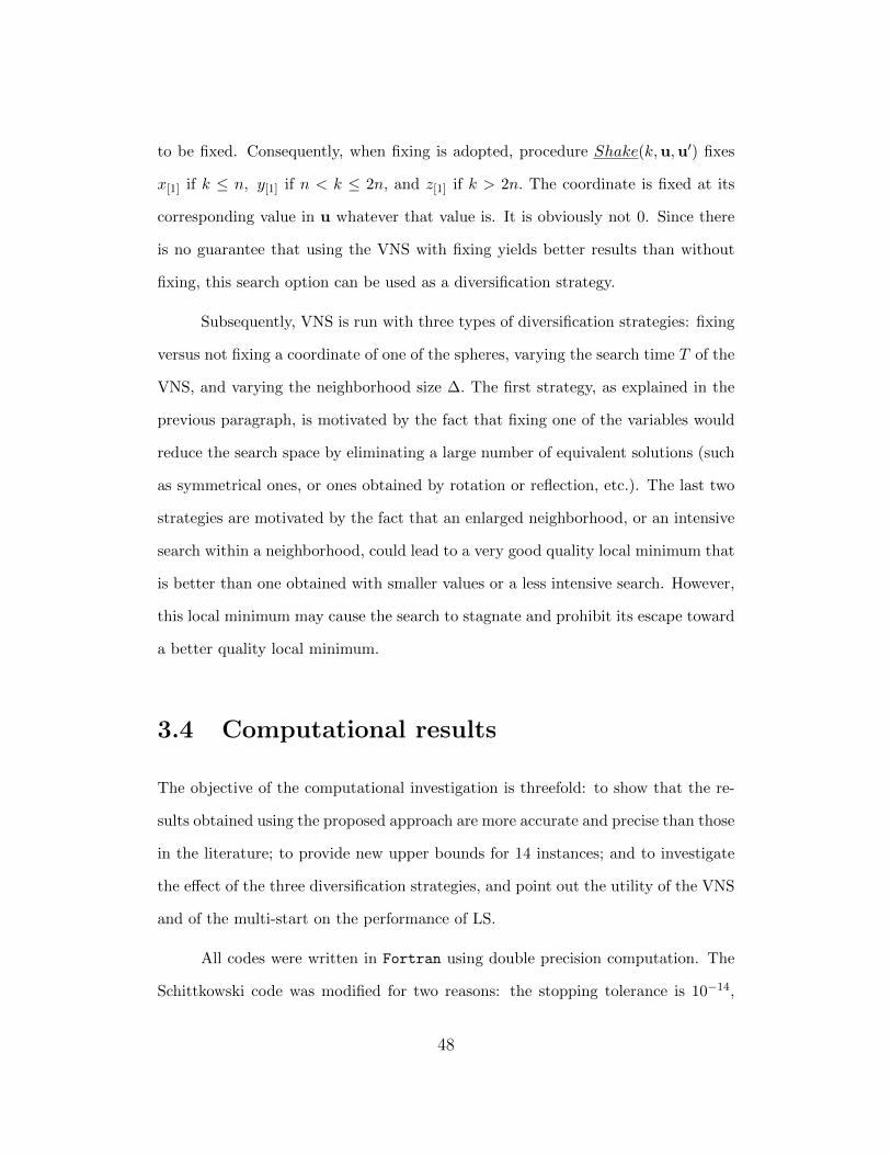
to be fixed. Consequently, when fixing is adopted, procedure Shake(k,u,u′) fixes

x[1] if k ≤ n, y[1] if n < k ≤ 2n, and z[1] if k > 2n. The coordinate is fixed at its

corresponding value in u whatever that value is. It is obviously not 0. Since there

is no guarantee that using the VNS with fixing yields better results than without

fixing, this search option can be used as a diversification strategy.

Subsequently, VNS is run with three types of diversification strategies: fixing

versus not fixing a coordinate of one of the spheres, varying the search time T of the

VNS, and varying the neighborhood size ∆. The first strategy, as explained in the

previous paragraph, is motivated by the fact that fixing one of the variables would

reduce the search space by eliminating a large number of equivalent solutions (such

as symmetrical ones, or ones obtained by rotation or reflection, etc.). The last two

strategies are motivated by the fact that an enlarged neighborhood, or an intensive

search within a neighborhood, could lead to a very good quality local minimum that

is better than one obtained with smaller values or a less intensive search. However,

this local minimum may cause the search to stagnate and prohibit its escape toward

a better quality local minimum.

3.4 Computational results

The objective of the computational investigation is threefold: to show that the re-

sults obtained using the proposed approach are more accurate and precise than those

in the literature; to provide new upper bounds for 14 instances; and to investigate

the effect of the three diversification strategies, and point out the utility of the VNS

and of the multi-start on the performance of LS.

All codes were written in Fortran using double precision computation. The

Schittkowski code was modified for two reasons: the stopping tolerance is 10−14,

48

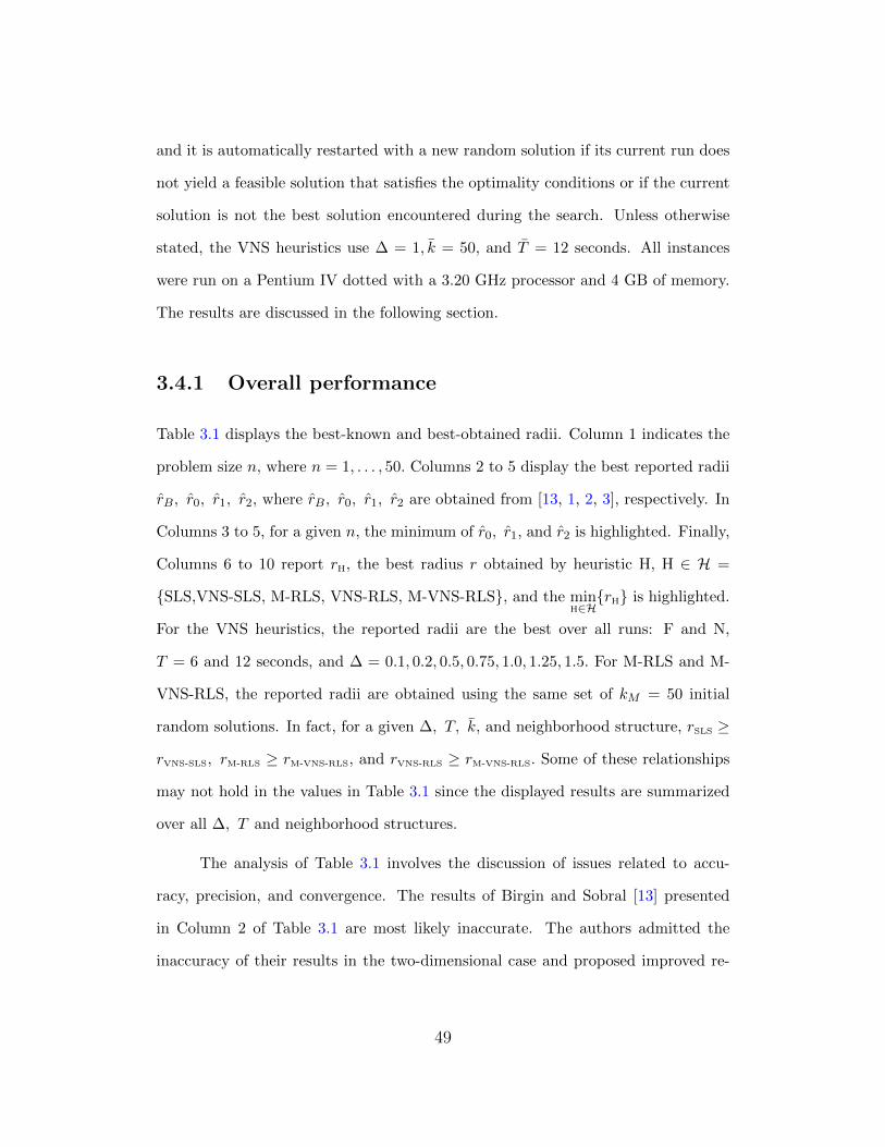
and it is automatically restarted with a new random solution if its current run does

not yield a feasible solution that satisfies the optimality conditions or if the current

solution is not the best solution encountered during the search. Unless otherwise

stated, the VNS heuristics use ∆ = 1, k = 50, and T = 12 seconds. All instances

were run on a Pentium IV dotted with a 3.20 GHz processor and 4 GB of memory.

The results are discussed in the following section.

3.4.1 Overall performance

Table 3.1 displays the best-known and best-obtained radii. Column 1 indicates the

problem size n, where n = 1, . . . , 50. Columns 2 to 5 display the best reported radii

rB, r0, r1, r2, where rB, r0, r1, r2 are obtained from [13, 1, 2, 3], respectively. In

Columns 3 to 5, for a given n, the minimum of r0, r1, and r2 is highlighted. Finally,

Columns 6 to 10 report rH, the best radius r obtained by heuristic H, H ∈ H =

{SLS,VNS-SLS, M-RLS, VNS-RLS, M-VNS-RLS}, and the minH∈H{rH} is highlighted.

For the VNS heuristics, the reported radii are the best over all runs: F and N,

T = 6 and 12 seconds, and ∆ = 0.1, 0.2, 0.5, 0.75, 1.0, 1.25, 1.5. For M-RLS and M-

VNS-RLS, the reported radii are obtained using the same set of kM = 50 initial

random solutions. In fact, for a given ∆, T, k, and neighborhood structure, rSLS ≥

rVNS-SLS, rM-RLS ≥ rM-VNS-RLS, and rVNS-RLS ≥ rM-VNS-RLS. Some of these relationships

may not hold in the values in Table 3.1 since the displayed results are summarized

over all ∆, T and neighborhood structures.

The analysis of Table 3.1 involves the discussion of issues related to accu-

racy, precision, and convergence. The results of Birgin and Sobral [13] presented

in Column 2 of Table 3.1 are most likely inaccurate. The authors admitted the

inaccuracy of their results in the two-dimensional case and proposed improved re-

49

Tab

le3.

1:B

est

Loca

lM

inim

an

rB

r0

r1

r2

rSL

SrV

NS-S

LS

rM

-RL

SrV

NS-R

LS

rM

-VN

S-R

LS

11.0

000005143

21.9

999202433

2.0

0000000000000

2.0

0000000000000

2.0

0000000000000

2.0

0000000000000

2.0

0000000000000

32.1

546210616

2.1

547006

2.1

547006

2.1

5470053824456

2.1

5470053824456

2.1

5470053837444

2.1

5470053837425

2.1

5470053837425

42.2

246870768

2.2

247450

2.2

247451

2.4

1421356237309

2.2

2474487138673

2.2

2474487138940

2.2

2474487138675

2.2

2474487138670

52.4

141267898

2.4

142139

2.4

142139

2.4

1421356237298

2.4

1421356236821

2.4

1421356237147

2.4

1421356236832

2.4

1421356236814

62.4

141694573

2.4

142139

2.4

142139

2.5

2752523165194

2.4

1421356237177

2.4

1421356237309

2.4

1421356237130

2.4

1421356236983

72.5

911991946

2.5

912543

2.5

912536

2.6

1368668160301

2.6

1368668160195

2.6

1368668160301

2.6

1368668160200

2.6

1368668159921

82.6

452822222

2.6

453291

2.6

453291

2.7

3205080757142

2.7

3205080756874

2.7

3205080756888

2.7

3205080756887

2.7

3205080756886

92.7

320034623

2.7

320516

2.7

320508

2.7

4182565152031

2.7

3205080756797

2.7

3205080756887

2.7

3205080756831

2.7

3205080756539

10

2.8

324167450

2.8

324648

2.8

324648

2.8

3246456105392

2.8

3246456105390

2.8

3246456105391

2.8

3246456105391

2.8

3246456105391

11

2.9

019556947

2.9

021140

2.9

021132

2.9

0211303259061

2.9

0211303259030

2.9

0211303259030

2.9

0211303259030

2.9

0211303259013

12

2.9

020105031

2.9

021140

2.9

021132

2.9

9941691897225

2.9

0211303259025

2.9

0211303259030

2.9

0211303259030

2.9

0211303258981

13

2.9

997977416

3.0

000003

3.0

000003

3.1

0221395734388

2.9

9999999999943

2.9

9999999999997

2.9

9999999999945

2.9

9999999999936

14

3.0

910230631

3.0

911462

3.0

911462

3.1

1144281851829

3.0

9114544488870

3.0

9114544488871

3.0

9114544488870

3.0

9114544488861

15

3.1

415101582

3.1

416438

3.1

416429

3.1

416409

3.3

2152692721521

3.1

4164262494870

3.1

4164262494871

3.1

4164262494871

3.1

4164262494867

16

3.2

155339532

3.2

156843

3.2

156833

3.2

156822

3.2

2035762742487

3.2

1568303201004

3.2

1568303201004

3.2

1568303201004

3.2

1568303201004

17

3.2

711271196

3.2

712462

3.2

712451

3.2

712451

3.3

1921100101264

3.2

9680836874176

3.2

9684043850944

3.2

9680836874176

3.2

9680836874176

18

3.3

188360708

3.3

189898

3.3

189898

3.3

189953

3.4

3690158448033

3.3

8084090740455

3.3

8084090740455

3.3

8084090740455

3.3

8084090740455

19

3.3

858513801

3.3

860164

3.3

860164

3.3

860198

3.5

5861664021641

3.4

6435524031985

3.4

6116202704004

3.4

6435524031985

3.4

6116202704004

20

3.4

733633429

3.4

735405

3.4

735405

3.4

740195

3.5

9742989177187

3.5

6548622298350

3.5

7187266979232

3.5

6548622298350

3.5

6548622298350

21

3.4

862092764

3.4

863528

3.4

863528

3.4

863492

3.6

2033409540338

3.6

0153022804217

3.6

0153022804217

3.6

0153022804217

3.6

0153022804217

22

3.5

796881818

3.5

800655

3.5

800655

3.5

799437

3.6

8953464150661

3.6

4051666844219

3.6

4051666844219

3.6

4051666844219

3.6

4051666844219

23

3.6

273889908

3.6

275165

3.6

275165

3.6

352929

3.7

6703739927985

3.7

6703739927985

3.7

6804140699504

3.7

6654989681805

3.7

6654989681805

24

3.6

852536176

3.6

853955

3.6

853955

3.6

854675

4.2

2574928847579

3.8

3281214836974

3.8

3289514992629

3.8

3281214836974

3.8

3281214836974

25

3.6

872896999

3.6

874285

3.6

874271

3.6

884037

4.0

4050812837879

4.0

4050812837879

3.6

8839179615006

3.7

5327834408109

3.6

8839179615006

26

3.7

471886302

3.7

474293

3.7

474054

3.7

498238

4.3

9215002079962

4.3

9080038824415

3.7

4740577652750

3.7

4740577652750

3.7

4740577652750

27

3.8

132974881

3.8

134171

3.8

134157

3.8

150465

4.4

6410161513775

4.4

6410161513775

3.8

1615120368277

3.8

4660056076369

3.8

1615120368277

28

3.8

415149358

3.8

417093

3.8

416399

3.8

447343

4.0

5290053391191

3.8

4164027814771

3.8

4177917884272

3.8

4164027814771

3.8

4164027814771

29

3.8

769556364

4.0

334762

3.8

770885

3.8

786901

3.9

0588517026782

3.8

7708910315835

3.8

7747914930252

3.8

7708910315835

3.8

7708910315835

30

3.9

163640724

3.9

165002

3.9

164910

3.9

249549

3.9

3900318427918

3.9

1649166155428

3.9

1654074598313

3.9

1649166155428

3.9

1649166155428

31

3.9

506163857

3.9

507874

3.9

507546

3.9

507734

4.0

1340436656033

3.9

5075448490565

3.9

5136931193641

3.9

5075448490565

3.9

5075448490565

32

3.9

873139176

3.9

874412

3.9

874412

3.9

886404

4.2

7254890158653

3.9

8744038931492

3.9

9772008339166

3.9

8744038931492

3.9

8744038931492

33

4.0

197789249

4.0

207406

4.0

199001

4.0

208602

4.0

8580036058113

4.0

1990091595852

4.0

1994758165121

4.0

1990091595852

4.0

1990091595852

34

4.0

475629785

4.0

478914

4.0

477194

4.0

484847

4.1

0040899215648

4.0

4771997123058

4.0

4944723850525

4.0

4771997123058

4.0

4771997123058

35

4.0

842793950

4.0

844935

4.0

844050

4.0

854179

4.1

3002114560296

4.0

8440574075337

4.0

8444990930670

4.0

8440574075337

4.0

8440574075337

36

4.1

128778440

4.1

129904

4.1

129887

4.1

358717

4.3

0716585797470

4.1

1298932968653

4.1

1298932968653

4.1

1298932968653

4.1

1298932968653

37

4.1

546179855

4.1

559012

4.1

547805

4.1

590245

4.2

4424648243793

4.1

5478125199120

4.1

5658310328267

4.1

5478125199120

4.1

5478125199120

38

4.1

575074608

4.1

577500

4.1

577345

4.1

604260

4.2

3715102793316

4.1

5766926004822

4.1

5773497480818

4.1

5766926004822

4.1

5766926004822

39

4.2

238096708

4.2

273985

4.2

239505

4.2

247035

4.2

5333789139973

4.2

3907241802319

4.2

5486395699313

4.2

2394975626618

4.2

2394975626618

40

4.2

551873286

4.2

557610

4.2

553336

4.2

576563

4.3

8558965541323

4.2

7145569016750

4.2

9321652173874

4.2

6365269398190

4.2

6365269398190

41

4.2

961778465

4.2

980380

4.2

963465

4.2

973417

4.3

1673932506242

4.3

1499920733667

4.3

2646345045588

4.3

1409218937400

4.3

0805958902068

42

4.3

080119020

4.3

132916

4.3

081351

4.3

081351

4.3

7739382983185

4.3

4481244093924

4.3

6786365788228

4.3

5355395885825

4.3

3740094016591

43

4.3

528504653

4.3

603289

4.3

528792

4.3

541301

4.3

9892791988379

4.3

7938295264594

4.4

0770331022630

4.3

8261922568558

4.3

7711338192368

44

4.3

827055183

4.3

829161

4.3

828335

4.3

843688

4.6

3248403341084

4.4

3037520199247

4.4

3643887928122

4.4

0321999967785

4.4

0321999967785

45

4.4

068820245

4.4

103145

4.4

070026

4.4

131795

4.4

9709897273965

4.4

6784626453004

4.4

6170130820936

4.4

5527185482123

4.4

4323242599026

46

4.4

409860772

4.4

421523

4.4

411264

4.4

412073

4.5

4196325546583

4.5

0305842563616

4.5

0219963456297

4.4

7847363222525

4.4

7847363222525

47

4.4

739825106

4.4

746333

4.4

741328

4.4

774382

4.5

9256828247835

4.5

2534868057796

4.5

4766625099119

4.5

4502187645631

4.5

1745560770452

48

4.4

961576629

4.4

973331

4.4

962836

4.4

971511

4.7

4031835202101

4.5

7213881540195

4.6

0308683627023

4.5

7449980224184

4.5

5711696552466

49

4.5

191083524

4.5

265746

4.5

192613

4.5

252964

4.8

3383651985818

4.6

1638412473422

4.6

6024661415626

4.6

6004684175310

4.6

1507723897088

50

4.5

504157703

4.5

589573

4.5

505657

4.7

6300934968712

4.6

9158717299905

4.7

4017473378151

4.7

0703758917657

4.6

6922650552785

50

sults for circle packing [12]. Because they used the same algorithm for packing unit

spheres, their results are probably erroneous. For example, when packing two unit

spheres into the smallest sphere, the authors obtain rB = 1.9999202433 while the

correct exact answer should be 2.0000000000. Similarly, when packing 13 circles,

rB = 2.9997977416, while the correct answer should be 3.0000000000. Thus, no

comparison will be undertaken with respect to these results.

The radii r0, r1, and r2 may lack some precision. They were obtained by

mapping the solution of equal sphere packing problem (ESPP) to the solution of

SPP. ESPP yields, in general, less precise solutions than SPP because of computa-

tional errors due to truncation and their faster rate of propagation for values that

are less than 1. However, as this chapter makes no attempt to assess these er-

rors, it is assumed that the precision of r0 and r1 is 10−7 (even though it could be

suspected that it does not exceed 10−6 since r0 = r1 = 3.0000003 for n = 13). Let

r = min{r0, r1, r2}. Evidently, r has the same precision as the least precise of r0, r1,

and r2. On the other hand, rH, H ∈ H, are suspected to be precise to 10−13, as can

be inferred from rH, H ∈ H, for n = 13. A valid comparison of rH to r requires either

truncating or rounding off rH to 10−7. However, regardless of the adopted compari-

son method, the proposed approach improves r for n = 3− 6, 9− 14, 31, 32, 38, and

39.

Finally, in many instances, starting LS with a non-feasible solution causes it

to stop the search and return an infeasible solution. The number of random initial

solutions that needed to be investigated prior to obtaining one that led to a local

minima reached 517 in one instance. This number was, however, much less in most

instances and averaged 7 for the kM iterations of M-RLS over and 3 per neighbor

for the VNS based heuristics over all runs.

Table 3.2 is a summary of Table 3.1. It reports the number of times rH is

51

less than rH’, (H,H’) ∈ (H ∪ {H1, H2, H3})2, with the diagonals giving the number

of times H is the only heuristic where in the best upper bound is obtained, and the

number in parentheses is the number of times H reaches the best upper bound but

is not the only heuristic where it is attained. It highlights the role of the VNS in the

search. Most of the best solutions are obtained using VNS based heuristics. In fact,

both SLS and M-RLS rarely outperform the VNS heuristics. Table 3.2 further shows

that M-VNS-RLS is the best heuristic; that is, its multi-start strategy coupled with

its variable neighborhood search allowed it to reach local minima that are closer to

the global minimum than the other proposed heuristics.

Table 3.2: Number of Times rH < rH’

↓ rH rH’ −→ rSLS rVNS-SLS rM-RLS rVNS-RLS rM-VNS-RLS r0 r1 r2rSLS 0(1) 0 6 1 1 5 4 0rVNS-SLS 44 1(4) 35 16 3 22 15 10rM-RLS 42 7 0(0) 4 1 18 12 9rVNS-RLS 47 12 34 0(4) 0 24 16 12rM-VNS-RLS 47 28 37 23 0(4) 24 16 13r0 43 26 30 24 24 0(3) 0 21r1 44 33 36 32 32 32 13(5) 29r2 35 25 26 23 22 14 4 3(2)

3.4.2 Feasibility of the initial solution

Table 3.2 shows that the number of times rM-RLS < rSLS is 42 whereas the number

of times rSLS < rM-RLS is only 6 (corresponding to n = 3, 23, 25, 39, 41, 43). This

discrepancy is expected and should be interpreted with care since rM-RLS is the best

radius over kM runs of LS; though, it remains true that starting LS from a feasible

solution is not always necessary. For example, the cases where n = 26 and 27

require that LS be started from a very good quality solution. In fact, starting them

from a feasible solution constructed using our naive approach leads to radii that

52

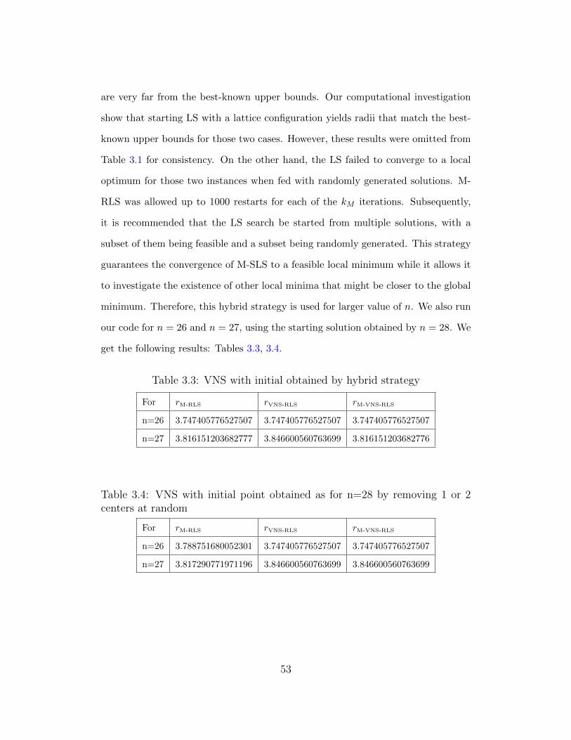
are very far from the best-known upper bounds. Our computational investigation

show that starting LS with a lattice configuration yields radii that match the best-

known upper bounds for those two cases. However, these results were omitted from

Table 3.1 for consistency. On the other hand, the LS failed to converge to a local

optimum for those two instances when fed with randomly generated solutions. M-

RLS was allowed up to 1000 restarts for each of the kM iterations. Subsequently,

it is recommended that the LS search be started from multiple solutions, with a

subset of them being feasible and a subset being randomly generated. This strategy

guarantees the convergence of M-SLS to a feasible local minimum while it allows it

to investigate the existence of other local minima that might be closer to the global

minimum. Therefore, this hybrid strategy is used for larger value of n. We also run

our code for n = 26 and n = 27, using the starting solution obtained by n = 28. We

get the following results: Tables 3.3, 3.4.

Table 3.3: VNS with initial obtained by hybrid strategy

For rM-RLS rVNS-RLS rM-VNS-RLS

n=26 3.747405776527507 3.747405776527507 3.747405776527507

n=27 3.816151203682777 3.846600560763699 3.816151203682776

Table 3.4: VNS with initial point obtained as for n=28 by removing 1 or 2centers at random

For rM-RLS rVNS-RLS rM-VNS-RLS

n=26 3.788751680052301 3.747405776527507 3.747405776527507

n=27 3.817290771971196 3.846600560763699 3.846600560763699

53

3.4.3 Utility of the diversification strategies

The first diversification strategy consists in varying ∆. Figures 3.3 to 3.8 illustrate

the impact is running when the VNS heuristics with and without fixing a coordinate

of one of the spheres. They display 1rH, H ∈ {VNS-SLS, VNS-RLS, M-VNS-RLS},

as a function of n for different neighborhood sizes (measured in terms of ∆). They

confirm the importance of varying ∆ in many instances such as n=13, 19-21, 24,

31, 37, 40, 45-49 of Figure 3.3. However, there is no general rule of thumb on how

to select the “best” ∆ value. Opting for a larger neighborhood is not necessarily

better than using a smaller one. Investigating a large neighborhood is equivalent

to too much perturbation of the current feasible solution (which itself corresponds

to a local minima). In fact, large perturbations induce “large” infeasibility (i.e.,

overlap). When the VNS heuristics are run without fixing a coordinate of one of

the spheres, opting for small ∆ values seems more judicious (in the instances where

the size of the neighborhood matters). In such cases, using ∆ = 0.1 and 0.2 seem

reasonable. However, none of these values of consistently dominate the others. This

rule holds when the VNS heuristics are run with the coordinate of one of the spheres

being fixed in all instances, except for n = 24 in Figure 3.6.

The second diversification strategy entails in varying T. Starting from the

same initial solution, each VNS heuristic H ∈ {VNS-SLS, VNS-RLS, M-VNS-RLS}

was run twice: once with T = 6 and once with T = 12. Let r(6)H and r

(12)H denote

the respective resulting radii. The results are summarized in Table 3.5; column 1

indicates whether the algorithms are run with or without fixing a coordinate of one

of the spheres. Columns 2 and 3 specify the neighborhood size ∆ and the heuristic

H. Columns 4-6 display η1, η2, η3, the number of times r(12)H > r

(6)H , r

(12)H = r

(6)H ,

and r(12)H < r

(6)H , respectively. Column 7 reports η4 the number of times H fails to

54

 

0.20

0.25

0.30

0.35

0.40

0.45

0.50

05

1015

2025

3035

4045

50

1/r H

n

Δ =

0.1

Δ =

0.2

Δ =

0.5

Δ =

1.0

Fig

ure

3.3:

Impac

tof

the

nei

ghb

orhood

size

onV

NS-S

LS

N.

55

 

0.20

0.25

0.30

0.35

0.40

0.45

0.50

05

1015

2025

3035

4045

50

1/r H

n

Δ =

0.1

Δ =

0.2

Δ =

0.5

Δ =

1.0

Fig

ure

3.4:

Impac

tof

the

nei

ghb

orhood

size

onV

NS-R

LS

N.

56

 

0.20

0.25

0.30

0.35

0.40

0.45

0.50

05

1015

2025

3035

4045

50

1/r H

n

Δ =

0.1

Δ =

0.2

Δ =

0.5

Δ =

1.0

Fig

ure

3.5:

Impac

tof

the

nei

ghb

orhood

size

onM

-VN

S-R

LS

N.

57

0.20

0.25

0.30

0.35

0.40

0.45

0.50

05

1015

2025

3035

4045

50n

1/r H

Δ =

0.1

Δ =

0.2

Δ =

0.5

Δ =

1.0

Fig

ure

3.6:

Impac

tof

the

nei

ghb

orhood

size

onV

NS-S

LS

F.

58

0.20

0.25

0.30

0.35

0.40

0.45

0.50

05

1015

2025

3035

4045

50n

1/r H

Δ =

0.1

Δ =

0.2

Δ =

0.5

Δ =

1.0

Fig

ure

3.7:

Impac

tof

the

nei

ghb

orhood

size

onV

NS-R

LS

F.

59

0.20

0.25

0.30

0.35

0.40

0.45

0.50

05

1015

2025

3035

4045

50n

1/r H

Δ =

0.1

Δ =

0.2

Δ =

0.5

Δ =

1.0

Fig

ure

3.8:

Impac

tof

the

nei

ghb

orhood

size

onM

-VN

S-R

LS

F.

60

identify a feasible solution when T = 6. Finally, Columns 8 and 9 report the average

and maximum deviations of r(6)H from r

(12)H over the cases with r

(6)H < r

(12)H whereas

the last two columns report the average and maximum deviations of r(12)H from r

(6)H

over the cases with r(12)H < r

(6)H .

Results in Table 3.5 suggest that varying ∆ can be successfully used as a diver-

sification strategy of VNS. Using T = 6 yields more frequent better-quality solutions

than using T = 12. However, the average and maximum improvements brought up

by using T = 12 when r(12)H < r

(6)H are more sizeable than their counterparts when

r(12)H = r

(6)H .

The cases when the magnitude of T does not affect the solution quality are

numerous, and the number is more important when H is run with a fixed coordinate

than when it is not fixed and for ∆ = 1.0 than for ∆ = 0.5. It also depends on the

heuristic H (most probably on the quality of the initial solution fed to H).

When ∆ = 1.0, the VNS heuristics fail in 35% of the instances to identify a

feasible solution when T = 6, for either the F or N versions of the algorithm. This

percentage is twice as large (16%) for the F version than for the N version (8%)

when ∆ = 0.5. This suggests that using ∆ = 1.0 while fixing a coordinate of one of

the spheres may result in infeasibility that cannot be resolved by the VNS within

the preset time limit T = 6; hence, none of the solutions fed to LS would yield a

feasible solution.

The third diversification strategy consists in running each of the VNS heuris-

tics twice: starting from the same initial solution, H ∈ {VNS-SLS, VNS-RLS, M-

VNS-RLS}, and run once with and once without fixing a coordinate of one of the

spheres; denoted by HF and HN respectively. The results are summarized by Ta-

ble 3.6 . Columns 1 and 2 specify the neighborhood size ∆ and the heuristic H.

61

Tab

le3.

5:Im

pac

tof

T

r(12)

H−r(6)

Hr(6)

H−r(12)

H

∆H

η1

η2

η3

η4

Avera

ge

Maxim

um

Avera

ge

Maxim

um

F0.5

VN

S-S

LS

23

14

74

0.0

006797964315658

0.0

047150070802350

0.0

000057821374355

0.0

001696240956520

VN

S-R

LS

23

14

74

0.0

010415722555616

0.0

075134699484810

0.0

000000000000015

0.0

000000000000300

M-V

NS-R

LS

34

93

40.0

008022943553068

0.0

065668290765730

0.0

000128310629656

0.0

005645667703930

F1.0

VN

S-S

LS

11

12

617

0.0

009741013792953

0.0

207184337198160

0.0

000000000000051

0.0

000000000000590

VN

S-R

LS

14

96

17

0.0

006410612097868

0.0

032101243210140

0.0

000000000000094

0.0

000000000001630

M-V

NS-R

LS

617

617

0.0

000494666703618

0.0

010025105653920

0.0

000000000000058

0.0

000000000001470

N0.5

VN

S-S

LS

14

17

57

0.0

001868529703426

0.0

027082005313520

0.0

000249052585654

0.0

008965893082480

VN

S-R

LS

16

15

57

0.0

005693284342984

0.0

039924776935160

0.0

007489865918569

0.0

267949192430750

M-V

NS-R

LS

14

17

57

0.0

0020905116113104

0.0

02094714645463

0.0

000088700368954

0.0

003193213279810

N1.0

VN

S-S

LS

812

716

0.0

001266946270644

0.0

012782688071870

0.0

000502741971153

0.0

005316148398080

VN

S-R

LS

422

116

0.0

002157503380220

0.0

022734007341170

0.0

000000000000004

0.0

000000000000100

M-V

NS-R

LS

519

316

0.0

000000000000043

0.0

000000000000820

0.0

000000000000043

0.0

000000000001070

62

Columns 3 to 5 display η1, η2, η3, the number of times rHN < rHF , rHF = rHN ,

and rHN > rHF , respectively. Column 6 reports η4, the number of times the VNS

heuristic fails to identify a feasible solution. Finally, Columns 8 and 9 report the

average and maximum deviations rHN − rHF when rHF < rHN , whereas Columns 10

and 11 give the average and maximum deviations rHF − rHN when rHF > rHN .

These results show that fixing the coordinate of one of the spheres is neither

always preferable nor undesirable. In fact, the maximum deviations of |rHF − rHN |

can reach 0.012: a very important variation for the problem at hand. Subsequently,

in many instances, reducing the search space (with the objective of eliminating

symmetry and related issues) is not advisable. Thus, a successful search strategy

should opt for testing both approaches of the problem, as is further elucidated by

the detailed results for HF and HN in Table 3.7.

3.4.4 Utility of the VNS and the LS

The best radii obtained by HF and HN when ∆ = 0.5 and T = 12 is given in Table

3.7. Column 1 indicates the problem size n. Columns 2 and 3 display rSLS and

rM-RLS. Columns 3 to 5 report rFH, the best radius r obtained by heuristic HF, H

∈ {VNS-SLS, VNS-RLS, M-VNS-RLS}, whereas Columns 6 to 8 display the same

information but for HN.

The result in Table 3.7 confirm that initiating LS from a feasible solution

always yields a local minimum. This is obviously not the case for infeasible so-

lutions. For instance, in the 48 instances tested above, LS failed to reach a local

minimum when started from a large set of randomly generated solutions. It is also

showed that the LS obtains a better solution when started with a feasible solution

in ten out of 48 instances, with the maximum deviation of rSLS from rM-RLS reaching

63

Tab

le3.

6:Im

pac

tof

Fix

ing

aC

oor

din

ate

ofO

ne

ofth

eSpher

esrH

N−rH

FrH

F−rH

N

∆H

η1

η2

η3

η4

Avera

ge

Maxim

um

Avera

ge

Maxim

um

1.0

VN

S-S

LS

19

15

10

40.0

004974439053977

0.0

077303518392241

0.0

000902961122576

0.0

038619636613130

VN

S-R

LS

22

11

11

40.0

008949954878760

0.0

066950721342630

0.0

003042420018562

0.0

124798832617420

M-R

LS-V

NS

17

21

64

0.0

002361300859217

0.0

018611165082080

0.0

000094867061752

0.0

004174150713850

0.5

VN

S-S

LS

23

18

52

0.0

008214480754788

0.0

080898502012480

0.0

000780921804996

0.0

034180268264650

VN

S-R

LS

22

16

82

0.0

011552657855988

0.0

097252610557670

0.0

000134694644134

0.0

004769662880320

M-R

LS-V

NS

30

11

52

0.0

008658800087198

0.0

065668290765730

0.0

000190941435287

0.0

008172609000440

64

Tab

le3.

7:E

ffec

tof

Fix

ing

the

Pos

itio

nof

aSpher

eon

the

Qual

ity

ofth

eSol

uti

onw

ith

∆=

0.5

andT

=12

Wit

hfi

xin

gW

ithout

fixin

gn

rSL

SrM

-RL

SrV

NS-S

LS

rV

NS-R

LS

rM

-VN

S-R

LS

rV

NS-S

LS

rV

NS-R

LS

rM

-VN

S-R

LS

32.1

5470053824456

2.1

5470053837475

2.1

5470053824456

2.1

5470053837425

2.1

5470053837425

2.1

5470053824456

2.1

5470053837425

2.1

5470053837425

42.4

1421356237309

2.2

2474487139144

2.2

2474487138673

2.2

2474487138675

2.2

2474487138675

2.2

2474487138693

2.2

2474487138683

2.2

2474487138681

52.4

1421356237298

2.4

1421356237147

2.4

1421356236963

2.4

1421356236839

2.4

1421356236831

2.4

1421356236870

2.4

1421356236878

2.4

1421356236823

62.5

2752523165194

2.4

1421356237309

2.4

1421356237253

2.4

1421356237243

2.4

1421356237094

2.4

1421356237227

2.4

1421356237169

2.4

1421356237055

72.6

1368668160301

2.6

1524242091076

2.6

1368668160272

2.6

1368668160289

2.6

1368668160243

2.6

1368668160219

2.6

1368668160295

2.6

1368668160281

82.7

3205080757142

2.7

3205080756888

2.7

3205080756887

2.7

3205080756887

2.7

3205080756887

2.7

3205080756887

2.7

3205080756887

2.7

3205080756887

92.7

4182565152031

2.7

3205080756887

2.7

3205080756858

2.7

3205080756884

2.7

3205080756793

2.7

3205080756874

2.7

3205080756887

2.7

3205080756668

10

2.8

3246456105392

2.8

3246456105556

2.8

3246456105391

2.8

3246456105391

2.8

3246456105391

2.8

3246456105391

2.8

3246456105391

2.8

3246456105391

11

2.9

0211303259061

2.9

0211303259030

2.9

0211303259030

2.9

9999999999989

2.9

0211303259030

2.9

0211303259030

2.9

9999999999982

2.9

0211303259030

12

2.9

9941691897225

2.9

0211303259030

2.9

0211303259030

2.9

9999999999975

2.9

0211303259030

2.9

0211303259030

2.9

9999999999981

2.9

0211303259030

13

3.1

0221395734388

3.0

0000000000000

3.0

9114544488871

2.9

9999999999991

2.9

9999999999972

3.0

9114544488871

2.9

9999999999981

2.9

9999999999950

14

3.1

1144281851829

3.0

9736179246790

3.0

9736179246790

3.0

9114544488871

3.0

9114544488871

3.0

9114544488871

3.0

9114544488871

3.0

9114544488867

15

3.3

2152692721521

3.1

4164262494871

3.1

5220026555598

3.1

4164262494871

3.1

4164262494871

3.1

4164262494870

3.1

4164262494871

3.1

4164262494871

16

3.2

2035762742487

3.2

1588315803967

3.2

1588315803967

3.2

1588315803967

3.2

1588315803967

3.2

1588315803967

3.2

1588315803967

3.2

1568303201004

17

3.3

1921100101264

3.2

9684043850944

3.2

9715029402540

3.3

2517878952614

3.2

96840438509440

3.2

9715029402540

3.2

9680836874176

3.2

9680836874176

18

3.4

3690158448033

3.3

8251273518736

3.3

8473980290167

3.3

8352323931557

3.3

8084090740455

3.3

8473980290167

3.3

8352323931557

3.3

8084090740455

19

3.5

5861664021641

3.4

7786806710072

3.5

0649304551939

3.5

3539962883257

3.4

6435524031985

3.4

6435524031985

3.4

7364779702559

3.4

6116202704004

20

3.5

9742989177187

3.5

7665233706004

3.5

7317588015077

3.5

8020224117702

3.5

6548622298350

3.5

7487212110729

3.5

8020224117701

3.5

7365883198394

21

3.6

2033409540338

3.6

1070943656382

3.6

2030787516073

3.6

3568047804109

3.6

1070943656382

3.6

0153022804217

3.6

3363147125231

3.6

0153022804217

22

3.6

8953464150661

3.6

4051666844219

3.6

4192954910622

3.6

4051666844219

3.6

4051666844219

3.6

4051666844219

3.6

4192955447838

3.6

4051666844219

23

3.7

6703739927985

3.7

6879846847560

3.7

6703739927985

3.7

6654989681805

3.7

6654989681805

3.7

6703739927985

3.7

6654989681805

3.7

6654989681805

24

4.2

2574928847579

3.8

3289514992629

3.8

3289390622137

3.8

3289390622137

3.8

3281214860800

3.8

3289390622137

3.8

3289390622137

3.8

3281214860673

25

4.0

4050812837879

4.1

8881752094069

4.0

4050812837879

4.0

4050812837879

4.0

4050812837879

4.0

4050812837879

4.0

4050812837879

4.0

4050812837879

26

4.3

9215002079962

4.3

9080038861019

27

4.4

6410161513775

28

4.0

5290053391191

3.8

5938265121346

3.8

6582129025475

3.8

4677122436886

3.8

4677122436886

3.8

4677122436886

3.8

4677122436886

3.8

4509642706231

29

3.9

0588517026782

3.8

8966248881778

3.8

7839027754598

3.9

0457084552566

3.8

7843617135428

3.8

7843617135428

3.9

0457084552566

3.8

7708910315835

30

3.9

3900318427918

3.9

2445917487543

3.9

2746450746635

3.9

9162636103909

3.9

1649166155428

3.9

2746450746635

3.9

4982913114897

3.9

1649166155428

31

4.0

1340436656033

3.9

7113053380349

4.0

1340436655556

3.9

8850892264477

3.9

5088896242510

3.9

6727513653610

3.9

7331290576204

3.9

5099049486861

32

4.2

7254890158653

4.0

0894046081310

4.0

0764532440897

4.0

2906991302087

4.0

0188284558907

3.9

9661151602936

4.0

1262649482391

3.9

9650463579512

33

4.0

8580036058113

4.0

2697939807711

4.0

2405977925337

4.0

2513119188639

4.0

2513119188639

4.0

2288135207819

4.0

2513119188639

4.0

1990091595852

34

4.1

0040899215648

4.0

4944723850525

4.0

8482441338340

4.0

7683683181969

4.0

4944723850525

4.0

5908254156022

4.0

7045397857175

4.0

4771997123058

35

4.1

3002114560296

4.0

8444990930670

4.1

0582201819603

4.1

1682595453275

4.0

8444990930670

4.0

9432596421864

4.1

1682595453275

4.0

8440574075337

36

4.3

0716585797470

4.1

4241224205426

4.1

1383912694139

4.1

3981328995080

4.1

2914477837374

4.1

1383912694139

4.1

3385293937593

4.1

1298932968653

37

4.2

4424648243793

4.1

6096800652210

4.2

3241893670340

4.1

6096800652210

4.1

5696571952974

4.2

3208477038344

4.1

5478125199120

4.1

5478125199120

38

4.2

3715102793316

4.2

3461234366052

4.2

3597802016207

4.2

3461234366052

4.2

2333755081395

4.2

3448099686564

4.1

5773497480818

4.1

5766926004822

39

4.2

5333789139973

4.2

7151398035863

4.2

5034151073013

4.2

6513995084063

4.2

4536170211884

4.2

5034151073013

4.2

6513995084063

4.2

3938145003991

40

4.3

8558965541323

4.3

4224220302311

4.3

1860576096985

4.3

2455096836581

4.2

7706783885791

4.2

8741505000694

4.2

6746039311058

4.2

6746039311058

41

4.3

1673932506242

4.3

7544223244230

4.3

1499920733667

4.3

7213616597835

4.3

2849297421721

4.3

1499920733667

4.3

5904934368174

4.3

0884069402462

42

4.3

7739382983185

4.3

8859740716231

4.3

7738425016750

4.3

9107436026373

4.3

6554388773070

4.3

7485649842280

4.3

7541322421017

4.3

5524264727754

43

4.3

9892791988379

4.4

2059573559044

4.3

8208253229267

4.4

1932860365510

4.3

9755136379951

4.3

8208253229267

4.4

1934200836812

4.3

9806052837831

44

4.6

3248403341084

4.4

3832644664312

4.4

6592125867765

4.4

4088832161426

4.4

3832644664312

4.4

5745720730599

4.4

4565798449458

4.4

0388868867003

45

4.4

9709897273965

4.4

8132644812954

4.4

6921272862671

4.4

8128019704679

4.4

6641782049140

4.4

6921272862671

4.4

6350443991294

4.4

5075663296053

46

4.5

4196325546583

4.6

2091267720554

4.5

1531840602923

4.6

2091267720554

4.4

9999576911328

4.5

0636205851480

4.5

8303242931251

4.4

8035842049339

47

4.5

9256828247835

4.5

4766625099119

4.5

7260789490155

4.5

4703260392380

4.5

4703260392380

4.5

2777880318190

4.5

4703260392380

4.5

3556984245498

48

4.7

4031835202101

4.6

5073005954271

4.5

9521585427709

4.6

8197552549096

4.5

9623053636001

4.5

8977916293008

4.5

8472291493329

4.5

5711696552466

49

4.8

3383651985818

4.7

0368559799948

4.7

2170144421721

4.7

1557841838051

4.6

6875731783470

4.6

4080294220473

4.7

1386677809460

4.6

2051643160067

50

4.7

6300934968712

4.7

4017473378151

4.6

9376374175179

4.7

6893782316805

4.7

2622078855716

4.7

2794401001644

4.7

6209491853735

4.6

8541082329544

Num

ber

of

tim

esrF H<rN H

58

5

Num

ber

of

tim

esrN H<rF H

23

22

30

65

0.148309392561900. On the other hand, LS obtains a better solution when started

from randomly generated solutions in 36 out of 48 instances with the maximum de-

viation being 0.392854138549501. It seems therefore judicious to include an initial

feasible solution among the solutions investigated by LS to guarantee its conver-

gence to a local optimum and its improved overall performance.

3.4.5 Comparison of the diversification strategies

VNS-SLS versus SLS

As expected, rSLS ≥ rVNS-SLS. Applying VNSF to the local optimum obtained by SLS

improved rSLS in 44 out of 48 instances. The improvement reaches 0.392855382254420,

and averages 0.055338061287952 over the 48 instances. Similarly, VNSN improves

rSLS in 43 out of 48 instances. The improvement reaches 0.392855382254420, and

averages 0.063762149389844 over the 48 instances.

VNS-RLS versus VNS-SLS

VNSF-RLS yields better solutions than VNSF-SLS in 25 out of 48 instances, with

the maximum deviation of rVNS-SLS from rVNS-RLS reaching -0.105594271176310.

The opposite case occurs in 16 instances with the maximum deviation equaling

0.091145444888800. The overall average deviation is -0.013753483385387. Simi-

larly, VNSN-RLS yields better solutions than VNS-SLS in 27 out of 48 instances,

with the maximum deviation of rVNS-SLS from rVNS-RLS reaching -0.097886967409520.

The opposite case occurs in 12 instances with the maximum deviation equaling

0.091145444888900. The overall average deviation is -0.010181470957522. This

suggests that VNS should be started from a feasible solution when not used in con-

66

junction with a multi-start strategy.

VNS-RLS versus M-RLS

The hybridization of VNS and LS can provide a powerful search method if it ad-

dresses the two competing goals of meta-heuristics: exploration and exploitation.

Exploration allows an extensive search of the solution space in order to determine

the part of the space that has a higher chance of containing the global optimum

whereas exploitation refines the search and focuses on the part of the space that

has a high potential of containing the global optimum. Exploration can be herein

obtained via multi-start or via VNS whereas exploitation is obtained via LS. Both

the multi-start and VNS strive for global optimization while LS strives for local

optimization in the global optimum neighborhood. The effectiveness of using VNS

and multi-start as the diversification strategies is discussed here.

The findings presented in Table 3.7 does not provide a clear answer to this

dilemma. It suggests using a mixture of the two search strategies. In fact, rFVNS-RLS <

rFM-RLS in 22 out 48 instances, while rF

VNS-RLS > rFM-RLS in 18 out 48 instances. The

maximum deviation in the first case equals -0.148309392561900 while it equals

0.097886967409590 in the second case. Its average is 0.004562699793446. Simi-

larly, rNVNS-RLS < rN

M-RLS in 28 out 48 instances while rNVNS-RLS > rN

M-RLS in 15 out 48

instances. The maximum deviation in the first case equals -0.148309392561900 while

it equals 0.097886967409520 in the second case. Its average is -0.006120725568965.

These different magnitudes of improvement over all instances of both versions of

the algorithms suggest that both diversification and intensification of the search are

important; one dose not predominate the other in any case.

M-VNS-RLS versus VNS-RLS

67

Comparison of Columns 5 and 6 and Columns 8 and 9 of Table 3.7 highlights the

importance of the diversification of the search by starting VNS-RLS from a number

of randomly generated solutions. In fact, the additional investigation brings forth

sizeable improvements. For VNSF, an improvement is registered in 32 out of 48

instances with the maximum improvement reaching 0.120916908092260 and averag-

ing 0.021911628194197 over the 48 instances. The same trend is observed for VNSN

where an improvement is registered in 37 out of 48 instances with the maximum im-

provement reaching 0.102674008819120 and averaging 0.019515894278337 over the

48 instances.

M-VNS-RLS versus M-RLS

Comparison of Column 3 to Columns 6 and 9 of Table 3.7 quantifies the importance

of diversifying the search by applying VNS to each of the kM local optima obtained

by M-RLS. The larger the discrepancy between rM-VNS-RLS and rM-RLS, the more im-

portant the role of VNS is, in identifying the global optima. For VNSF, an improve-

ment is observed in 36 out of 48 instances with the maximum improvement reaching

0.148309392561900 and averaging 0.014861185920063 over the 48 instances. Simi-

larly, for VNSN, an improvement is observed in 42 out of 48 instances with the max-

imum improvement reaching 0.148309392561900 and averaging 0.022481100856624

over the 48 instances.

3.5 Conclusion

A variable neighborhood search approach is proposes in this chapter, to solve the

problem of packing n unitary spheres into the smallest containing sphere S where

the objective is to identify the radius of S and a feasible configuration of the uni-

68

tary spheres within S. The approach follows the recent research trends of combining

search heuristics with non-linear programming tools and of balancing exploitation

and exploration. Indeed, it ensures exploitation by applying a local search based

on a sequential quadratic programming algorithm with a non-monotone line search

(as a non-linear programming solver) and exploration by applying a variable neigh-

borhood search and a multi-start strategy. The approach provides accurate results

with a precision of 10−13. It can be extended to the case of non-identical spheres

and to the packing of spheres into other 3-dimensional shapes.

69

Chapter 4

Packing Spheres in a Cube

4.1 Introduction

In this chapter, the adaptation of the VNS to the problem of packing sphere in

a cube is explored. An introduction to the VNS has been given in section 2.1 of

chapter 2, so we will not repeat its rules here.

Sphere packing in a cube is an optimization problem, that could be classified

either as continuous and or as discrete. The positions of the spheres are presented

in continuous variables, whereas the structure of an optimal configuration is discrete

[49]. A successful solution technique should tackle these two aspects simultaneously.

Accordingly, we approximately solve the problem of packing unit spheres into

the smallest cube (PSC) using a variable neighborhood search (VNS) that combines

these two aspects. A VNS addresses the discrete aspect of the PSC by shaking one

or more spheres and its continuous aspect by applying a non-linear programming

(NLP) optimizer that identifies a local optimum within the neighborhood of the fed

solution. In addition, it yields local optima that are nearer to the global optimum,

70

in a more straightforward manner than do other meta-heuristics. The VNS has

successfully been applied to solve many problems, including integer and continuous

optimization problems [52].

For 3D packing of spheres the literature is not as extensive as for solving

correspond 2D packing. However, it is clear that mathematical programming for-

mulations could easily be extended from 2D to 3D. As far as we know, there is only

one journal paper considering 3D packing of spheres into a cube by Birgin and So-

bral [13]. The authors considered the objects in different shapes as triangle, circle,

square and strips. More detailed description of their work is given in chapter 3.

Other two references that we will use in computational results to compare with, we

take from websites [4, 5] that just report the best known values. However, it is not

clear what methods they used to report those values.

4.2 Mathematical model

PSC comprises of packing n identical spheres, of radius one, without overlap into

the smallest containing cube C. The goal is to search for the best packing of the n

spheres into C, where the best packing minimizes w, the length of the side of C.

According to the typology of Wascher et al. [79], PSC is a three-dimensional variant

of the Open Dimension Problem, since all small items (which are spheres) have to

be packed and the extension of the large object (which is a cube) is not given but

has to be minimized. PSC is equivalent to finding the coordinates (xi, yi, zi) of every

sphere i, i = 1, . . . , n, and the side w of C. There are several equivalent nonlinear

programming formulations of PSC. The simplest one is given in Costa et al. [7]

where objective is to maximize the small radius of sphere.

71

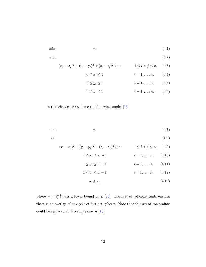
min w (4.1)

s.t. (4.2)

(xi − xj)2 + (yi − yj)2 + (zi − zj)2 ≥ w 1 ≤ i < j ≤ n, (4.3)

0 ≤ xi ≤ 1 i = 1, . . . , n, (4.4)

0 ≤ yi ≤ 1 i = 1, . . . , n, (4.5)

0 ≤ zi ≤ 1 i = 1, . . . , n, . (4.6)

In this chapter we will use the following model [13]

min w (4.7)

s.t. (4.8)

(xi − xj)2 + (yi − yj)2 + (zi − zj)2 ≥ 4 1 ≤ i < j ≤ n, (4.9)

1 ≤ xi ≤ w − 1 i = 1, . . . , n, (4.10)

1 ≤ yi ≤ w − 1 i = 1, . . . , n, (4.11)

1 ≤ zi ≤ w − 1 i = 1, . . . , n, (4.12)

w ≥ w, (4.13)

where w = 3

√43πn is a lower bound on w [13]. The first set of constraints ensures

there is no overlap of any pair of distinct spheres. Note that this set of constraints

could be replaced with a single one as [13]:

72

n−1∑i=1

n∑j=i+1

max{0, 4− (xi − xj)2 − (yi − yj)2 − (zi − zj)2} = 0, (4.14)

The next three sets (4.10 - 4.12) ensure the containment of every sphere within C.

PSC assumes that the bottom leftmost lowest of C coincides with the origin

(0; 0; 0). PSC has an in infinite number of alternative optima caused by symmetrical

configurations. Fixing the position of one of the spheres would reduce the search

space by eliminating a large number of equivalent solutions [8, 16, 17, 45, 61], with-

out necessarily loosing subspaces including good quality local optima. Herein, we

set two of the coordinates of a randomly chosen sphere to 1 so that the solver main-

tains this sphere adjacent to two edges of the cube during its search. Additional

bounding constraints that lexicographically ordered the spheres were investigated

but not adopted in this model. Solving PSC via an NLP solver only is generally not

successful [5]. Subsequently, PSC is solved by VNS.

4.3 Variable neighborhood search-based algo-

rithm for the PSC problem

The proposed VNS is to solve the PSC problem detailed in Algorithm 2. It is in fact

very similar to one described in chapter 3 for solving PSS. It starts its search from

a feasible solution u = (x1, y1, z1, . . . , xn, yn, zn) for PSC with a side length wu. The

coordinates of u by randomly generating by using uniform distribution from the

interval (1, 2 3√n). Any overlapping spheres are moved to out-skirt of C. VNS sets

the best solution u∗ = u, and its upper bound w∗u = wu. It initializes its cumulated

73

runtime t is 0 and k = 1.

Algorithm 2 Detailed Algorithm of the VNS for PSC

Input

1 A feasible solution u = (xi, yi, zi)i=1,...,n, and wu its side length of C.

2 T, the maximal runtime for VNS.

3 k, the maximal number of neighborhoods.

Output

1 A (near-) optimal solution u∗ = (x∗i , y∗i , z∗i )i=1,...,n, and its side length wu∗ .

Algorithm

1 Set u∗ = u and wu∗ = wu.

2 Set the algorithm’s cumulated runtime t to 0.

3 Do while t ≤ T

3.1 Set the neighborhood type k = 1.

3.2 Do while k ≤ k

3.2.1 Generate a random solution u′ from the kth neighborhood Nk(u) of u.

3.2.2 Starting from u′, find a local minimum u” and its side length wu”.

3.2.3 If wu” < wu,set k = 1, u = u”, and wu = wu”;if wu” < wu∗ , set u∗ = u”, and wu∗ = wu”.

Elseset k = k + 1.

3.2.4 Update t.

The VNS is an iterative procedure with two loops. The outer loop controls

the runtime whereas the inner one undertakes the search. At each iteration of the

inner loop, the VNS generates a random solution u′ from a neighborhood Nk(u)

74

of u. It finds a local minimum u” ∈ Nk(u) by applying NLP to the PSC starting

from u′. The selected NLP solver is NLPQLP, a sequential quadratic programming

algorithm with a non-monotone line search [63]. The NLPQLP is designed for

smooth NLP problems. When the solver aborts because of computational errors

caused by inaccurate function or gradient evaluations, a non-monotone line search

is activated. Internal restarts are performed in case of errors when computing the

search direction due to inaccurate derivatives. Additional automated initial and

periodic scaling with restarts are implemented [63].

If wu” < wu, the current solution u is updated; i.e., the focus of the search is

re-centered on u”, and k is reset to 1. Furthermore, if wu” < wu∗ , then wu∗ is reset

to wu”, and u∗ to u”.

On the other hand, if wu” ≥ wu, the neighborhood of u; i.e., k is incremented.

A random solution u′ ∈ Nk(u) is chosen, and the local optimum u” within Nk(u)

is identified. The neighborhood is enlarged until one of the two stopping criteria is

met:

∗ A solution u” ∈ Nk(u) such that wu” < wu is obtained; in which case, k is reset

to 1 and the inner loop is repeated.

∗ The number of investigated neighborhoods k reaches the threshold k; in which

case the algorithm’s total runtime t is updated and the control of the algorithm

is transferred to the outer loop of the VNS.

The outer loop is the stopping criterion of the VNS. It compares t to the

maximum runtime allowed T. VNS stops when t exceeds T.

The iterative step generates a solution u′ from a neighborhood Nk(u), k =

1, . . . , k, of u using a shaking procedure. For k = 1, this procedure translates one

randomly chosen sphere by δx, δy and δz in the x, y and z directions, respectively.

75

For 1 < k < k, the procedure translates the min{n2 , k} randomly chosen spheres

in the x, y and z directions, respectively. Finally, when k = min{k, n − 1}, it

moves the k closest neighbors of a randomly chosen sphere; thus inducing variations

on the position of a cluster of spheres. The parameter k is set experimentally to

min{n2 , 6}. In all cases, the translation distances are randomly generated from the

Uniform[−∆,∆], where ∆ is the neighborhood parameter. If a translation causes

the violation of the lower (resp. upper) bound of a variable, this latter is reset at

its lower (resp. upper) bound. The shaking procedure is very useful since it offers

multiple starts for NLPQLP; thus, enhances its chances of identifying a (near-)

global optimum.

4.4 Computational results

In this section we provide computational results obtained by our method for solving

PSC problem. This section will be much smaller in size than one in chapter 3, since

we use experience from extensive computational analysis from chapter 3. In other

words, we use variant of the model with fixing the cube centre, assuring that all

variables are nonnegative. As a nonlinear solver, we use NLPQLP [63]. Further, we

use here the better initial solution method from there. We generate random initial

solution for equivalent maximization of small circle problem. In order to preserve

feasibility, the initial value of r is set to 0.001. The transformation to minimization

problem is then performed to be in appropriate form for the model we use. For the

parameter ∆ we always use value 0.5. The value of VNS parameter T is again set

to 6 seconds for each independent run. Each test instance is run 10 times and best

values reported. The value of k is chosen as min{n, 50}.

The results are presented at Table 4.1. Column 1 indicates the problem size

76

Table 4.1: Comparing the Best Local Minima to the Best Known Radii

n wB w wP w∗

3 3.4141527373 3.4142137817 3.4142135624 3.4142135624

4 3.4141480640 3.4142137817 3.4142135624 3.4142135624

5 3.7887647862 3.7888547050 3.7888543820 3.7888543820

6 3.8855478230 3.8856182776 3.8856180832 3.8856180832

7 3.9977338382 3.9978227857 3.9978227238 3.9978227238

8 3.9999345267 4.0000000000 4.0000000000 4.0000000000

9 4.3093402273 4.3094012173 4.3094010768 4.3094010768

10 4.6666081946 4.6666669778 4.6666666667 4.6666666667

11 4.8159601052 4.8164394712 4.8164397406 4.8164397406

12 4.8280686639 4.8284278518 4.8284270236 4.8284270519

13 4.8282131208 4.8284278518 4.8284271247 4.8284271247

14 4.8282912625 4.8284278518 4.8284271247 4.8284271247

15 5.1997445225 5.1999997920 5.2000000000 5.2000000000

16 5.2964155013 5.2967013468 5.2967008293 5.2967008293

17 5.2996749577 5.2998313329 5.2998316455 5.2998316455

18 5.3279843248 5.3282026294 5.3282011774 5.3282011774

19 5.4586383844 5.4589562912 5.4589532170 5.4589532170

20 5.6048721029 5.6051549489 5.6051549576 5.6051549576

21 5.6431452803 5.6427342320 5.6427344101 5.6430934602

22 5.7710452688 5.7712362738 5.7712361663 5.7712361663

23 5.8199237336 5.8201577088 5.8201531911 5.8201531911

24 5.8633943713 5.8637080741 5.8637033052 5.8637033052

25 5.9589662351 5.9593423866 5.9593308221 5.9593308221

26 5.9952148260 5.9914286622 5.9914262468 5.9955822990

27 5.9998355203 6.0000006000 6.0000000000 6.0000000000

28 6.2421317695 6.2425479584 6.2425477277 6.2425477277

29 6.2423824504 6.2426414863 6.2426406871 6.2426406871

30 6.2424721518 6.2426414863 6.2426406871 6.2426406871

31 6.2425174557 6.2426414863 6.2426406871 6.2426406871

32 6.2425285827 6.2426414863 6.2426406871 6.2426406871

33 6.4689813902 6.4680814732 6.4680780465 6.4680780465

34 6.5735658875 6.5738915268 6.5738831658 6.5738831658

35 6.5931612342 6.5933290674 6.5933259094 6.5933259094

36 6.6970889746 6.6975333654 6.6944181198 6.6975126034

37 6.7083709308 6.7086358928 6.7086344826 6.7086344826

38 6.7093947495 6.7096644329 6.7096635745 6.7096635745

39 6.7739983433 6.7742714525 6.7742701172 6.7742701172

40 6.7998570644 6.8000010880 6.8000000000 6.8000000000

41 6.9039667243 6.9042869063 6.9042712513 6.9042712513

42 6.9906644142 6.9909219383 6.9907863116 6.9907863116

43 7.0610542561 7.0595743359 7.0595386299 7.0595386299

44 7.0991542522 7.0992323600 7.0992166891 7.0992166891

45 7.1269867567 7.1107596816 7.1107603214 7.1107603214

46 7.1396025069 7.1302925488 7.1302839201 7.1302839201

47 7.1447631846 7.1449572499 7.1449567477 7.1449574116

48 7.2254788705 7.1449572499 7.1449575543 7.1449575543

49 7.3396050716 7.3299434788 7.3299402906 7.3312658497

50 7.3606467872 7.3554452729 7.3554013072 7.3598400994

Average 5.8321665039 5.8296846262 5.8296132074 5.8298918455

51 7.4070535149 7.4061413497 7.4263293310

52 7.4727301395 7.4727224395 7.4729829434

53 7.5058057407 7.5057697640 7.5561707846

54 7.5967666642 7.5641117363 7.6046039060

55 7.6497254384 7.6402978341 7.6207736668 7.6392010852

n. Columns 2 , 3 and 4 display the side length wB , w and wP obtained by [13],

[4] and [5], respectively. Column 5 reports the side length w∗ obtained by VNS.

The configurations corresponding to wB are not necessarily feasible. They may

77

have overlapping spheres or spheres that are not totally contained within the cube.

Thus, wB will not be used for comparison purposes. For each instance of Table

4.1, the underlined value indicates the tightest upper bound. In column 4 we give

the currently best known solutions from web site Packomania. However, we did not

compare our results with those from Packomania, since they are obtained by many

different people and many different methods. Thus, although we report results

obtained by 3 different sources, we compare ours only with those from [4].

The following observations one can get from the results of Table 4.1: (i)

VNS improves the best solutions obtained by [4] in 35 out of 48 instances; it rep-

resents 73% of the cases. (ii) The best improvement of an existing upper bound is

0.0010967489 occurring for n = 55, with the improvement averaging 0.0000391436

over the 35 improved instances. These improvements are important despite their

seemingly small magnitude. (iii) Results obtained by [4] are of better quality for

large values of n. This clearly indicates that another parameter values for our VNS

should be chosen. That could be a task for the future work.

4.5 Conclusion

In this chapter we apply Variable neighbourhood search (VNS) approach for solving

sphere packing problem within smallest containing cube, in 3D. VNS is framework

for building heuristics. It starts from initial solution and use different neighbour-

hoods of that solution in order to improve it. The perturbation or shaking phase of

the current solution is obtained by moving k (k = 1, . . . , k) sphere centres for the ∆

(a parameter) in each dimension. As a local search it is used well-known software for

solving nonlinear convex problems [63]. It appears that 35 out of 48 better results

are reported when compared with current state of the art. Future work may contain

78

application of this approach to other packing problems in different containers. In

addition, better parameter estimation for large values of n could be performed.

79

Chapter 5

Conclusion

5.1 Summary

The Variable Neighborhood Search (VNS) is one of the most efficient general search

frameworks. It has several heuristic variations, and can easily be adapted to contin-

uous and discrete combinatorial problems. This thesis presents a tutorial along with

a detailed literature review on recent applications of the VNS and its variants. As

for other meta-heuristics, the hybridization of the VNS with other approximate or

exact search algorithms enhances its efficiency and efficacy. This thesis applies a hy-

brid VNS to approximately solve the problem of three-dimensional circular packing,

where the containing object is spherical or cubical and the items are unit spheres.

This problem is relevant to many real-life applications. A successful application of

a VNS-based heuristic requires a good definition of the representation of the solu-

tion, its neighbourhoods, its moves within a neighbourhood, and its local search.

In this context, the neighbourhood has a special structure since it is continuous

but disconnected. The proposed VNS implementation represents a solution by the

80

three-dimensional coordinates of its solutions and its solution value by the radius of

the containing sphere or by the length of the side of the containing cube. It generates

a neighbouring solution by shaking one or more spheres (depending on the neigh-

bourhood size). It applies a local search by applying the non-linear programming

search technique that had obtained a large percentage of best near-global optima

for other classes of complex problems while ensuring high precision. The proposed

heuristic is restarted a fixed number of times so that it benefits from the diversifica-

tion induced by different initial starting points. The computational results provide

computational proof of the efficiency and efficacy of the VNS-based heuristic. When

the containing object is a sphere, our best method is able to improve 60.4% of best

known solutions and matches all other results. When the containing object is a

cube, it improves 76.4% of existing solutions. Many of these solutions are suspected

to be optimal, and any improvement is due a large computational precision. Indeed,

the proposed approach has a higher precision level than most of the state-of-the-art

approaches.

5.2 Future research

Future research might include applying the VNS to the simpler two-dimensional

shapes or to more complex p-dimensional containers such as rectangular, triangu-

lar, pyramidal, and strip-shaped. Different variants of the problem may require

different neighbourhood structures and/or different moves. Future and undergoing

research concerns the augmentation and reduction of the problem via linearization

and reformulation techniques. In real life packing of spheres, optimizes space usage

is the most significant goal; yet, different issues are likewise considered. For exam-

ple, cargo steadiness, multi-drop loads or weight circulations are also pertinent and

81

should be considered during the packing or loading to ensure cargo security. Thus,

adding these constraints into the three-dimensional packing problem is imperative

for enhancing the applicability of this research. Such extensions could focus on

the efficiency of space usage, and mixing different types of items to fill these voids.

Finally, the proposed VNS heuristic could inspire the development of efficient com-

putational heuristics for continuous optimization in other areas such as engineering

and econometric.

82

Bibliography

[1] Hugo Pfoertner, Dense Packings of Equal Spheres in a Larger Sphere,available at www.randomwalk.de/sphere/insphr/sequences.txt, accessedon February 2011.

[2] Hugo Pfoertner, Dense Packings of Equal Spheres in a Larger Sphere,available at www.randomwalk.de/sphere/insphr/spisbest.txt, last ac-cessed on February 2011.

[3] Jerry Donovan, Boris Lubachevsky, and Ron Graham, Optimal Pack-ing Of Circles And Spheres, available at home.comcast.net/ dave-janelle/packing.html, accessed on February 2011.

[4] Hugo Pfoertner, Densest Packings of Equal Spheres in a Cube, available atwww.randomwalk.de/sphere/incube/spicbest.txt, last accessed on Febru-ary 2011.

[5] Eckhardt Specht, Packing equal spheres in a cube, available atwww.packomania.com, last accessed on August 2012

[6] Smart Wi-Fi for Warehouses, Ruckus Wireless, available athttp://c541678.r78.cf2.rackcdn.com/brochures/brochure_warehouse.pdf.

[7] A. Costa, P. Hansen, and L. Libert, “Bound constraints for Point Pack-ing in a Square”. International Conference on Operations Research andEnterprise Systems, (2012), pp. 5–10.

[8] A. Costa, P. Hansen, and L. Libert,“On the impact of symmetry-breakingconstraints on spatial Branch-and-Bound for circle packing in a square”.Discrete Applied Mathematics, (2013),161, pp. 96–106.

[9] A. Grosso, A. R. M. J. U.Jamali, and M. Locatelli, “Finding maximinlatin hypercube designs by Iterated Local Search heuristics”. EuropeanJournal of Operational Research, (2009),197, pp. 541–547.

[10] E. G. Baum, “Toward practical ‘neural’ computation for combinatorialoptimization problems,” Neural Networks for Computing,American Insti-tute of Physics, (1986).

[11] K. Bezdek “Sphere packings revisited.”European Journal of Combina-torics (2006); 27; pp. 864-883.

[12] E. G. Birgin, and J. M. Gentil, “New and improved results for packingidentical unitary radius circles within triangles,” Computers & OperationsResearch,(2010), 37, pp. 1318–1327.

83

[13] E. G. Birgin, and F. N. C. Sobral, “Minimizing the object dimensions incircle and sphere packing problems,” Computers & Operations Research,(2008), 35, pp. 2357–2375.

[14] M. Chiarandini, and T. Stutzle, “An application of iter-ated local search to the graph coloring problem,” Elec-tronic Notes in Discrete Mathematics, (2006),availabled athttp://www.cs.colostate.edu/ howe/cs640/papers/stutzle.pdf, accessedon June 2002.

[15] J.H. Conway, and N.J.A. Sloane, “Sphere Packings, Lattices, andGroups,” Springer-Verlag, New York, (1999).

[16] A. Costa, and L. Libert, “Formulation symmetries in circle packing”.Electronic Notes in Discrete Mathematics, (2010), 36, pp. 1303–1310.

[17] A. Costa, and I. Tseveendorj, “Symmetry breaking constraints for theproblem of packing equal circles in a sqaure”. The Cologne-Twente Work-shop on Graphs and Combinatorial Optimization, (2011), pp. 126–129.

[18] E. Burke, T. Curtois, M. Hyde, G. Kendall, G. Ochoa, S. Petrovic, J.Vazquez-Rodrguez, and M. Gendreau, “Iterated local search vs. hyper-heuristics: towards general-purpose search algorithms,” EvolutionaryComputation (CEC), (2010), Issue No. 978-1-4244-6909-3, pp. 1-8.

[19] F. Glover, and G. Kochenberger, Handbook of Metaheuristics, Glover F.and Kochenberger G. Kluwer, (2003).

[20] G. Kandavanam, D. Botvich, S. Balasubramaniam, and B. Jennings, “Ahybrid genetic algorithm/variable neighborhood search approach to maxi-mizing residual bandwidth of Links for route planning,” TSSG, WaterfordInstitute of Technology, Ireland, P. Collet et al. (Eds.): EA 2009, LNCS5975, (2010), pp. 49–60.

[21] G. Yaskov, Y. Stoyan, and A. Chugay, “Packing identical spheres intoa cylindrical domain,” Proceedings of the Workshop on Cutting StockProblems 2005 (WSCSP2005, September, 15-18 2005, Miercurea-Ciuc,Romania), Alutus, Miercurea-Ciuc, Romania, pp. 75-82, (2006).

[22] T. Gensane, “Dense packings of equal spheres in a cube,” Electronic Jour-nal of Combinatorics, (2004), 11, no. 1, R 33.

[23] H. R. Lourenco, O. Martin, and T. Stuetzle, “Iterated local search,”Glover F. and Kochenberger G. (eds.), Handbook of Metaheuristics,Kluwer, (2003), pp. 321–353.

[24] T. C. Hales, “A proof of the Kepler Conjecture,”Annals of Mathematics,(2005), 162(1), pp. 1065-1185.

84

[25] P. Hansen and N. Mladenovic, “An introduction to variable neighborhoodsearch,” S. Voss et al. eds., Metaheuristics, Advances and Trends in LocalSearch Paradigms for Optimization, Kluwer, (1999), pp. 433–458.

[26] P. Hansen , and N. Mladenovic, “Developments of variable neighbor-hood search”. In: Ribeiro C, Hansen P, editors. Essays and Surveys inMetaheuristics. Boston, Dordrecht, London: Kluwer Academic Publish-ers; (2001), pp. 415–440.

[27] P. Hansen , and N. Mladenovic, “Variable neighborhood search: principlesand applications”. European Journal of Operational Research, (2001);130:pp. 449–467.

[28] P. Hansen , and N. Mladenovic, “Variable neighborhood search”. In:Glover F,Kochenberger G, Handbook of metaheuristics. Boston, Dor-drecht, London: Kluwer Academic Publisher; (2003), pp. 145–184.

[29] P. Hansen , and N. Mladenovic, “Variable neighborhood search”. In: E. K.Burke, and G. Kendall (Eds), Search Methodologies: Introductory Tuto-rials in Optimization and Decision Support Techniques.Springer; (2005),pp. 211–238.

[30] P. Hansen , and N. Mladenovic, “Variable neighborhood search methods”.Les Cahiers du GERAD, G-2007-52,(2007).

[31] P. Hansen, and N. Mladenovic, “A Tutorial Variable Neighborhood Search”. Les Cahiers du GERAD, G-2003-46,(2003).

[32] M. Hifi, and R. M’Hallah, “A Literature Review of Circle and SpherePacking Problems: Models and Methodologies,” Advances in OperationsResearch, (2009) , Article ID 150624, 22 pages, doi:10.1155/2009/150624.

[33] M. Hurtgen, and J. C. Maun, “Optimal PMU placement using IteratedLocal Search”. Electrical Power and Energy Systems, (2010), 32, pp.857–860.

[34] J. Brimberg , P. Hansen , N. Mladenovic and E. Taillard, “Improvementsand Comparison of Heuristics for solving the Multisource Weber Prob-lem”. In: Operations Research, (2000), 48, pp. 444-460.

[35] J. Kratica, M. Leitner, and I. Ljubi, “Variable Neighborhood Search forSolving the Balanced Location Problem”. In: TECHNISCHE UNIVER-SITAT WIEN, Institut fur Computergraphik und Algorithmen, (2012),TR-186-1-12-01.

[36] J. Lazic, S. Hanafi, N. Mladenovic, and D. Urosevic, “Variable neighbour-hood decomposition search for 0-1 mixed integer programs”. ComputersOperations Research , (2010), 37, pp. 1055–1067.

85

[37] J. F. Liu, Y. L. Yao, Y. Zheng, H. T. Geng, and G. C. Zhou, “An effectivehybrid algorithm for the circles and spheres packing problems.”In: D. Z.Du, X. D. Hu, P. M. Pardalos (Eds), Combinatorial Optimization andApplications: Third International Conference. Berlin: Springer; (2009),pp. 135-144.

[38] J. Moreno-Perez, P. Hansen , and N. Mladenovic, “Parallel variable neigh-borhood search ”. Les Cahiers du GERAD, G-2004-92,(2004).

[39] L. F. Garcia, B. Melian Batista, J. A. Moreno Perez, and J. M. MorenoVega, “The parallel variable neighbourhood search for the P -median prob-lem”. Journal of Heuristics, (2002), 8, pp. 375–388.

[40] M. Hifi, and R. M’Hallah, “Beam search and non-linear programmingtools for the circular packing problem”. International Journal of Mathe-matics in Operational Research, (2009), 1, pp. 476–503.

[41] M. Hifi, and R. M’Hallah, “A dynamic adaptive local search based algo-rithm for the circular packing problem”. European Journal of OperationalResearch , (2007), 183, pp. 1280–1294.

[42] M. Gan, N. Gopinathan, X. Jia, and R. A. Williams, “Predicting packingcharacteristics of particles of arbitrary shapes,” KONA Powder & ParticleJournal, (2004), 22, pp. 82-93.

[43] M. Maric, Z. Stanimirovic, and N. Milenkovic, “Metaheuristic methods forsolving the Bilevel Uncapacitated Facility Location Problem with Clients’Preferences”. In Faculty of Mathematics, University of Belgrade, Ser-bia,Electric Notes in Discrete Mathematics, (2012), 39, pp. 43–50.

[44] N. Mladenovic, “A variable neighborhood algorithm-A new metaheuristicfor combinatorial optimization”. Presented at Optimization Days, Mon-treal , (1995), p. 112.

[45] N. Mladenovic , and P. Hansen, “Variable neighborhood search.’ Com-puters and Operations Research, (1997);24:1097–1100.

[46] N. Mladenovic, R. Todosijevic, and D. Urosevic, “An efficient generalvariable neighborhood search for large travelling salesman problem withtime windows”, Yugoslav Journal of Operations Research, (2012), 22, no.2.

[47] N. Mladenovic, J. Petrovic, V. Kovacevic-Vujcic, and M. Cangalovic“Solving spread spectrum radar polyphase code design problem by tabusearch and variable neighbourhood search”European Journal of Opera-tional Research, (2003), 151, pp. 389–399.

[48] N. Nikolic, Igor Grujicic, and Dorde Dugosija, “Variable neighborhooddescent heuristic for covering design problem”Electronic Notes in DiscreteMathematics, (2012), 39, pp. 193–200.

86

[49] P. R. J. Ostergard “Book review,”Computers and Operations Research,(2008), 36, pp. 276–278.

[50] P. Hansen, C. Oguz, and N. Mladenovic, “Variable neighborhood searchfor minimum cost berth allocation,”European Journal of Operational Re-search, (2008), 191, pp. 636–649.

[51] P. Hansen, N. Mladenovic, and J. Moreno-Perez, “Variable neighbour-hood search: methods and applications,”INVITED SURVEY, 4OR,(2008), 6, pp. 319–360.

[52] P. Hansen, N. Mladenovic, and J. Moreno-Perez, “Variable neighbour-hood search: methods and applications,”Annals of Operations Research,(2010), 175, pp. 367–407.

[53] P. Hansen, N. Mladenovic, and D. Perez-Brito, “Variable neighborhooddecomposition search”Journal of Heuristics, (2001), 7, pp. 335–350.

[54] P. Hansen, N. Mladenovic, and D. Urosevic “Variable neighborhoodsearch and local branching,”Computers & Operations Research, (2006),33, pp. 3034–3045.

[55] R. M’Hallah, and A. Alkandari , “Packing unit spheres into a cube usingVNS,” Electronic Notes in Discrete Mathematics, (2012), 39, pp. 201–208.

[56] R. M’Hallah, A. Alkandari, and N. Mladenovic, “Packing unit spheresinto the smallest sphere using VNS and NLP,” Computers OperationsResearch, (2013), 40, pp. 603–615.

[57] R. Qu, Y. Xu, and G. Kendall, “A Variable Neighborhood Descent SearchAlgorithm for Delay-Constrained Least-Cost Multicast Routing, In T.Stutzle (Ed.),” LION 3, LNCS 5851, Springer-Verlag, Berlin, Heidelberg,(2009), pp. 15–29.

[58] C. R. Reeves, “Modern heuristic techniques for combinatorial problems,”Blackwell Scientific Press, (1993).

[59] S. Brito, G. Fonseca, T. Toffolo, H. Santos, and M. Souza, “A SA-VNSapproach for the High School Timetabling Problem,” Electronic Notes inDiscrete Mathematics, (2012), 39, pp. 169-176.

[60] S. Hanafi, J. Lazic, and N. Mladenovic, “Variable neighbourhood pumpheuristic for 0–1 mixed integer programming feasibility,” Electronic Notesin Discrete Mathematics, (2010), 36, pp. 759–766.

[61] S. Kucherenkoa , P. Belottib , L. Libertic, and N. Maculand , “Newformulations for the Kissing Number Problem”, Discrete Applied Mathe-matics,(2007), 155, pp. 1837–1841.

87

[62] J. Sanchez-Oro, and A. Duarte, “An experimental comparison of Vari-able Neighborhood Search variants for the minimization of the vertex-cutin layout problems”. Electronic Notes in Discrete Mathematics,(2012),39,pp. 59–66.

[63] K. Schittkowski , “NLPQLP: A Fortran Implementation of a SequentialQuadratic Programming Algorithm with Distributed and Non-MonotoneLine Search - User’s Guide,”Report, Department of Computer Science,University of Bayreuth, (2010), V 3.1.

[64] R. Silva, and S. Urrutia, “A general VNS heuristic for the traveling sales-man problem with time windows ,” Discrete Optimization, (2010), 7, pp.203–211.

[65] Y. G. Stoyan, “Mathematical methods for geometric design,” in: Ad-vances in CAD/CAM: Proceedings of PROLAMAT82, Leningrad, USSR,16–18 May 1982, pp. 67–86. North-Holland, Amsterdam, (2003).

[66] Y. G. Stoyan, and G. Yaskov, “Packing Identical Spheres into a Rect-angular Parallelepiped,” In: A. Bortfeldt, J. Homberger, H. Kopfer, G.Pankratz, R. Strangmeier, Intelligent Decision Support. Current Chal-lenges and Approaches, Betriebswirtschaftlicher Verlar Dr. Th. Gabler,GWV Fachverlage GMbH, Wiesbaden, (2008), pp. 47-67.

[67] Y. G. Stoyan and G. N. Yaskov, “A mathematical model and a solu-tion method for the problem of placing various sized circles into a strip,”European Journal of Operational Research, (2004), 156, pp. 590-600.

[68] Y. G. Stoyan, and G. N. Yaskov, “Packing identical spheres into a right

circular cylinder,” Proceedings of the 5th ESICUP Meeting, L’Aquila,Italy, April 20 - 22, (2008).

[69] Y. G. Stoyan, and G. N. Yaskov “Packing congruent hyperspheres into ahypersphere,”Journal of Global Optimization, (2012), 52, pp. 855–868.

[70] A. Sutou, and Y. Dai, “Global optimization approach to unequal spherepacking problems in 3D,”Journal of Optimization Theory and Applica-tions, (2002), 114, No. 3, pp. 8671–694.

[71] Szabo, P. G., M. C. Markot, T. Csendes, E. Specht, L. G. Casado, andI. Garcia, New Approaches to circle Packing in a Square, Springer,NewYork (2007).

[72] T. G. Crainic, M. Gendreau, P. Hansen, and N. Mladenovic, “Coopera-tive parallel variable neighborhood search for the p -median,”Journal ofHeuristics, (2004), 10, pp. 293–314.

[73] M. Toksari, and E. Guner, “Solving the unconstrained optimization prob-lem by a variable neighborhood search,”Journal of Mathematical Analysisand Applications, (2007), 328, pp. 1178–1187.

88

[74] S. Torquato, and F. H. Stillinger, “Exactly solvable disordered sphere-packing model in arbitrary-dimensional Euclidean spaces,”Physical Re-view, (2006), E 73, pp. 031106–031114.

[75] J. Wang, “Packing of unequal spheres and automated radiosurgical treat-ment planning,” Journal of Combinatorial Optimization,(1999), 3, pp.453-463.

[76] S. R. Williams, and A. P. Philipse, “Random packing of spheres andsphero-cylinders simulated by mechanical contraction,” Physics Review,(2003), E 67, pp. 051301-051309.

[77] Y. G. Stoyan, G. N. Yaskov, and G. Scheithauer, “Packing of variousradii solid spheres into a parallelepiped,” Central European Journal ofOperational Research, (2003), 11, pp. 389-407.

[78] Y. G. Stoyan, J. Terno, G. Scheithauer, and T. Romanova, “Φ functionsfor primary 2D-objects,” Studia Informatica Universalis, InternationalJournal on Informatics, Special Issue on Cutting, Packing and Knap-sacking,(2002), 2, pp. 1-32.

[79] G. Wascher, H. Haussner, and H. Schumann, “An improved typologyof cutting and packing problems,” European Journal of Operational Re-search, Special Issue on Cutting and Packing,(2007), 183, no. 3, pp. 1109-1130.

[80] G. Zoutendijk, “Nonlinear Programming, Computational Methods, Inte-ger and Nonlinear Programming,” North Holland Publishing Co, Amster-dam,(1970).

89