the socio-economic marine research unit...
TRANSCRIPT

12-WP-SEMRU-05
For More Information on the SEMRU Working Paper Series
Email: [email protected], Web: www.nuigalway.ie/semru/
The Socio-Economic Marine Research Unit (SEMRU) National University of Ireland, Galway
Working Paper Series
Working Paper 12-WP-SEMRU-05
Exploring cost heterogeneity in recreational demand
Edel Doherty
Danny Campbell
Stephen Hynes
SEMRU Working Paper Series

12-WP-SEMRU-05
Exploring cost heterogeneity in recreational demand
Abstract
Farmland can confer significant public good benefits to society aside from its role in
agricultural production. In this paper we investigate preferences of rural residents for
the use of farmland as a recreational resource. In particular we use the choice
experiment method to determine preferences for the development of farmland walking
trails. Our modelling approach is to use a series of mixed logit models to assess the
impact of alternative distributional assumptions for the cost coefficient on the welfare
estimates associated with the provision of the trails. Our results reveal that using a
mixture of discrete and continuous distributions to represent cost heterogeneity leads
to a better model fit and lowest welfare estimates. Our results further reveal that Irish
rural residents show positive preferences for the development of farmland walking
trails in the Irish countryside.
.

1 Introduction
Farmland produces a wide range of private and public goods and services for
society. Many of the private benefits of farmland arise from the production of
food and fibre and other consumable goods that are exchanged in formal mar-
kets. Value is determined in these markets through exchange and quantified in
terms of price. On the other hand, environmental services and recreational ben-
efits produced by farmland create a range of public good benefits. Declining
agricultural activity coupled with policy emphasis on enhancing the public good
provision of farmland has led to a greater emphasis being placed on providing
the non-market benefits from farmland. Indeed, in Ireland, research has shown
that Irish farmland produces substantial non-market benefits, in addition to the
traditional role of agricultural production (Campbell, 2007; Hynes et al., 2011).
In particular, the role of farmland as a recreational resource is increasingly be-
ing recognised within Ireland (Buckley et al., 2009a) and beyond (Fleischer and
Tsur, 2000). In this context, this paper seeks to investigate Irish rural residents’
preferences for the provision of recreational walking trails on farmland.
There are a number of reasons for focusing on the demand for recreational
walking. First, among the general population of Ireland, walking is by far the
most common recreational activity. A study by Curtis and Williams (2005) found
that three-quarters of the Irish adult population participated in walking for recre-
ational purposes. Second, given the popularity of recreational walking, there is a
considerable body of evidence to suggest that walking activity has the potential
to generate significant revenue from both tourists and domestic residents (Failte,
2009; Fitzpatrick and Associates, 2005). For instance Fitzpatrick and Associates
(2005) estimated the direct expenditure, such as food and accommodation expen-
diture, of recreational trails and forest recreation at AC305 million annually while
the non-market benefits value of trails were estimated at AC95 million. Third,
Ireland’s most highly regarded walks are located in mostly rural regions of low
population densities where local economies have been in stagnation due to the
decline in agriculture (Buckley et al., 2008a). Buckley et al. (2008b) quanti-
fied the opportunity cost associated with recreation on farm commonage1. They
found that only 23 percent of farms showed a positive gross margin in a post-
decoupling scenario. They note that if the payment was removed the economics
of farming activity on marginal areas is questionable.
Hynes et al. (2007) argue that relative to traditional agricultural activities, out-
door recreation may represent a more economically efficient use of commonage
resources, albeit providing recreational access does not necessarily require farm-
ers to stop commercial farming. They note that policy-makers are recognising
the value of open-air outdoor recreational as a means of supporting rural in-
1Commonage refers to unenclosed land on which two or more farmers have pasture rights in
common (Lyall, 2000)
3

comes and the Rural Development Plan through niche tourism; environmentally
guided farming; rural diversification; job creation and rural regeneration. There-
fore, increasing provision of walking trails on farmland could help maximise
the potential of the recreational walking market as well as provide an alternative
means to sustain marginal rural regions. Finally, previous research by Buckley
et al. (2009a)—based on two farmland recreational sites in Connemara—found
support among walkers for more formalised walking trails.
Ireland is a particularly unique case study to examine the recreational walk-
ing benefits of farmland. This is because the rights of access to the countryside
belongs primarily to private landowners, who are mostly farmers. In this pa-
per we investigate preferences for the development of farmland walking trails
using the choice experiment (CE) method. CEs are a stated preference method-
ology widely used by practitioners in the field of environmental and resource
economics to derive estimates of willingness to pay (WT P) for environmental
non-market goods and services. The appeal of CEs lies in their ability to pro-
vide rich information on the preferences that individuals hold for environmental
goods and services. Additionally a wide array of random utility models are avail-
able from which CE data can be analysed. In this paper we employ a variety of
models that fall under the mixed logit umbrella. In particular we use various
specifications of the random parameters logit (RPL) model, which has the ability
to capture random taste variation.
For the RPL model, debate remains regarding how to appropriately accom-
modate random taste variation in estimation. In particular, what distributions
should be employed to represent the random taste heterogeneity. For derivation
of WT P from RPL models, two considerations are important. First, what dis-
tributions should be applied to the non-cost attributes representing a particular
environmental service. Second, what distribution should be assumed for the co-
efficient representing the cost attribute. Balcome et al. (2009) explored many
of these issues and found little support for fixing the cost coefficient, which to
date, has been a relatively common practice in the literature (e.g., Colombo et al.,
2007; Provencher and Bishop, 2004; Morey and Rossmann, 2008; Carlsson et al.,
2007; Bujosa et al., 2010). Indeed, Thiene and Scarpa (2009) call the assumption
of a fixed marginal utility of money across individuals, implied by a fixed cost
coefficient, heroic.
The main reason why a fixed cost coefficient is assumed in the literature is
because it has a number of convenient properties. For example, if the non-cost
coefficients are specified with a Normal distribution, then the distribution of the
mean and standard deviation of WT P is also Normal when the cost coefficient
is fixed. Therefore a fixed coefficient allows computationally straightforward
WT P estimates. A further reason why cost is held constant is that specifying
it as random can lead to extreme (negative and positive) estimates for marginal
WT P. Additionally, a model with a random cost attribute may not have well
4

defined moments (Balcome et al., 2009; Daly et al., Forthcoming). However, as
noted by Train and Weeks (2005) assuming a fixed cost coefficient implies that
the standard deviation of unobserved utility (the scale parameter) is the same
for all observations. Scarpa et al. (2008) note that in the context of recreational
choice, which is also the focus of this study, if the travel cost coefficient is fixed
when scale varies over observations then the variation in scale will be erroneously
attributed to variation in WT P for site attributes.
In this paper we investigate alternative specifications for the travel cost coef-
ficient in mixed logit models of recreational site-choice. We add to the literature
by exploring heterogeneity in the cost coefficient between a discrete, continuous
and a mixture of distributions (combining discrete and continuous distributions),
where the latter specification can accommodate multi-modality in preferences.
Other studies have explored the multi-modality of attribute heterogeneity (e.g.,
Wasi and Carson, 2011; Fosgerau and Hess, 2009; Fosgerau and Bierlaire, 2007;
Scarpa et al., 2008). In this paper we concentrate on alternative specifications for
cost only, as opposed to the non-cost attributes, given its paramount importance
in welfare estimation. This mirrors an interest within the literature on how to
represent the cost coefficient and obtain sensible WT P estimates. For instance, a
log-normal distribution can ensure that the distribution of cost is bounded below
zero, which ensures the theoretically plausible negative utility associated with
cost, yet practical applications have shown that it can lead to unusually large and
untenable WT P estimates (Train and Weeks, 2005). Furthermore, as shown by
Scarpa et al. (2008) the undesirable skewness of WT P distributions derived from
preference space model specifications based on random travel cost coefficients is
not eliminated by assuming bounded distributions. On the other hand, a number
of studies have shown that parametrising the model directly in WTP space pro-
vides estimates of WT P distributions that are more tenable and associated with
less extreme WT P values (Sonnier et al., 2007; Train and Weeks, 2005; Scarpa
et al., 2008; Balcome et al., 2009). As a result, in addition to our preference
space specifications, we investigate the impact of using a mixture of distribution
approach in WTP space, which to our knowledge, has not been previously exam-
ined within the literature. According to Daly et al. (Forthcoming) parametrising
models directly in WTP space also ensures finite moments for the WT P distribu-
tions. A noteworthy study by Torres et al. (2011) using Monte Carlo simulation,
found that mistaken assumptions about the cost parameter can amplify environ-
mental attribute mis-specification. They find that this may be due to assuming a
constant parameter on cost, rather than getting the distribution wrong, although
they note that results are sensitive to the size of the environmental changes being
valued.
The remainder of the paper is structured as follows. In the next section we
explain our econometric methodology. This is followed by a description of the
policy context for the research, survey design and implementation in section 3.
Section 4 presents and discusses the results. Finally section 5 presents the con-
5

clusions and policy recommendations arising from our findings.
2 Methodology
2.0.1 Preference Space Models
In this paper we explore the implications of different distributional assumptions
for the cost coefficient in mixed logit models. Starting with the conventional
specification of utility for the RPL model, where respondents are indexed by n,
chosen alternative by i in choice occasion t, the cost attribute by p and the vector
of non-cost attributes by x, we have:
Unit = −αpnit + β′xnit + ηnit + εnit, (1)
where pni and xni are the observed variables that relate to the cost and non-cost
attributes respectively, −α and β represent the coefficients for the cost and non-
cost attributes. η represents error components that induce correlations between
the designed alternatives (Scarpa et al., 2005; Campbell, 2007; Scarpa et al.,
2007). These are normally distributed with a zero mean and standard deviation
(σ2) so that η ∼ N(O, σ2) where ηnit is equal to zero for the status quo alternative
and ε is an iid Gumbel distributed error term. In the first model specification
considered in this paper we assume a fixed cost coefficient. For this model we
define θ to represent the combined vector of β and η so that the unconditional
choice probability for the RPL model, with random continuous cost and non-
cost attributes becomes.
Prob(yn) =
∫
θ
Tn∏
t=1
(
exp(−αpnit + β′xnit + ηnit)
∑
j exp(−αpn jt + β′xn jt + ηn jt)
)
f (θ)d(θ) (2)
where yn gives the sequence of choices over the Tn choice occasions for respon-
dent n, i.e. yn =⟨
in1, in2, . . . , inTn
⟩
.
A key element with the specification of random taste heterogeneity is the assump-
tion regarding the distribution of each of the random parameters (Hensher and
Greene, 2003). Random parameters can take a number of predefined functional
forms, such as, for example, Log-Normal, Normal or Triangular. Additionally,
more recent studies have gone beyond the assumption of unimodiality and allow
for multimodality distributions. Examples include the mixtures of normals ap-
proach (e.g., Fosgerau and Hess, 2009; Wasi and Carson, 2011) or mixture of
normals and log-normals (e.g., Fiebig et al., 2010; Hensher and Greene, 2011) or
the Legendre Polynomial as used by Fosgerau and Bierlaire (2007) and Scarpa
et al. (2008). Based on a priori expectations of the possible signs of the attributes,
6

we specify the heterogeneity for all of the non-cost attributes as having a Normal
distribution, β ∼ N (µ, σ), while we explore alternative specifications for the cost
coefficient.
In our second model specification we assume that the cost coefficient is rep-
resented by two discrete values, rather than remain fixed. In estimation this is
achieved by assigning α with m mass points, αm, each of mass points is asso-
ciated with a probability πm, with the condition that the combined probabilities
adds to one (Hess et al., 2007). In this case the unconditional choice probability
takes the following form:
Prob(yn) =
m∑
m=1
πm
∫
θ
Tn∏
t=1
(
exp(−αm pnit + β′xnit + ηnit)
∑
j exp(−αm pn jt + β′xn jt + ηn jt)
)
f (θ)d(θ)
(3)
In this model specification we segment the cost coefficient into two mass points,
each with an associated probability, while the remaining attribute coefficients are
each specified with a single continuous distribution. Using such a modelling ap-
proach represents somewhat of a hybrid between the RPL and latent class (LC)
models. This is because we have specified our non-cost attributes to follow a
continuous distribution as in the RPL model, while we have specified our cost at-
tribute to be represented by two finite values each with association probabilities,
which is common for LC models. The main difference between our specification
and the LC model is that we segment on a per parameter basis (in this case based
on the cost parameter) rather than on the basis of the full set of parameters which
is typical in LC models.
Notwithstanding the ability of the discrete mixtures (DM) approach to capture
some heterogeneity associated with the cost attribute, we also explore the poten-
tial of using a continuous distribution for cost, rather than assuming a fixed or
DM representation. In this case we can extend θ to represent the combined vec-
tor of α, β and η so that the unconditional choice probability for the RPL model,
with random continuous cost and non-cost attributes becomes
Prob(yn) =
∫
θ
Tn∏
t=1
(
exp(−αpnit + β′xnit + ηnit)
∑
j exp(−αpn jt + β′xn jt + ηn jt)
)
f (θ)d(θ) (4)
As with the non-cost attributes we once again use a normal distribution to capture
the heterogeneity associated with the cost coefficient, i.e., α ∼ N (µ, σ).
As noted by Bujosa et al. (2010), however, there may be a possible need for
more than one distribution to represent random heterogeneity. They note that in
the presence of different groups of individuals with different group specific tastes,
7

the RPL model might be inadequate2. Whilst assuming within group homogene-
ity, as represented by finite distributions, might be too stringent. As a result we
apply the mixtures of Normals approach to allow additional heterogeneity as-
sociated with each of two discrete points. This specification allows additional
flexibility in the specification of the cost coefficient compared to the other alter-
natives explored in this paper. Other studies that have applied the mixtures of
Normals approach include Wasi and Carson (2011), Fosgerau and Hess (2009)
and Boeri (2011). Similarly, Bujosa et al. (2010) and Hensher and Greene (2013)
extend the traditional latent class model with all fixed coefficients to a random
parameters latent class model, which enables within class preference heterogene-
ity.
Following Fosgerau and Hess (2009) we combine a standard continuous mix-
ture approach with a discrete mixture approach. Specifically, the mixing dis-
tribution is itself a discrete mixture of more than one independently distributed
Normal distribution. In the context of cost the approach would allow for two
groups of respondents based on their sensitivity to cost. One group may have
a strong dislike for higher prices (a highly price sensitive group), and the other
may have a low price sensitivity (and may be indifferent to the cost attribute),
while there may be additional cost heterogeneity associated with each subgroup.
If there is no additional heterogeneity associated with the cost coefficients within
each subgroup then the distributions are reflected by the standard DM approach
and the choice probability is represented by Equation 3.
For the mixture of distribution approach we combine Equation 3 and Equa-
tion 4 and the resulting choice probability becomes:
Prob(yn) =
m∑
m=1
πm
∫
θm
Tn∏
t=1
(
exp(−αm pnit + β′xnit + ηnit)
∑
j exp(−αm pn jt + β′xn jt + ηn jt)
)
f (θm)d(θm)
(5)
In this model we specify two mean parameters µm to represent the heterogeneity
surrounding the cost coefficient, and a correspondent set of standard deviations
σm. For each pair of parameters (µm, σm), we then define a probability, πm. The
resulting distribution allows for m separate modes, where the different modes
can differ in mass. As a result our cost attribute is represented by a combined
RPL-DM approach, which has both discrete points and continuous distributions.
Whilst our non-cost attributes have the same specification as the previous models
and are represented by the standard RPL approach.
2We have defined RPL models here narrowly to represent models that include unimodial
continuous distributions as represented by Equation 2 and Equation 4. As pointed out by a
reviewer, however, our definition is restrictive and narrow given that RPL models in principle
also includes discrete mixture models and is synonymous with Mixed Logit Models.
8
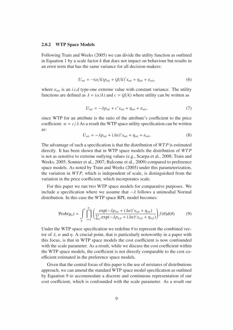
2.0.2 WTP Space Models
Following Train and Weeks (2005) we can divide the utility function as outlined
in Equation 1 by a scale factor k that does not impact on behaviour but results in
an error term that has the same variance for all decision-makers:
Unit = −(α/k)pnit + (β/k)′xnit + ηnit + εnit, (6)
where εnit is an i.i.d type-one extreme value with constant variance. The utility
functions are defined as λ = (α/k) and c = (β/k) where utility can be written as
Unit = −λpnit + c′xnit + ηnit + εnit, (7)
since WTP for an attribute is the ratio of the attribute’s coefficient to the price
coefficient: w = c/λAs a result the WTP space utility specification can be written
as:
Unit = −λpnit + (λw)′xnit + ηnit + εnit, (8)
The advantage of such a specification is that the distribution of WT P is estimated
directly. It has been shown that in WTP space models the distribution of WT P
is not as sensitive to extreme outlying values (e.g., Scarpa et al., 2008; Train and
Weeks, 2005; Sonnier et al., 2007; Balcome et al., 2009) compared to preference
space models. As noted by Train and Weeks (2005) under this parameterization,
the variation in WT P, which is independent of scale, is distinguished from the
variation in the price coefficient, which incorporates scale.
For this paper we run two WTP space models for comparative purposes. We
include a specification where we assume that −λ follows a unimodial Normal
distribution. In this case the WTP space RPL model becomes:
Prob(yn) =
∫
θ
Tn∏
t=1
(
exp(−λpnit + (λw)′xnit + ηnit)∑
j exp(−λpn jt + (λw)′xn jt + ηn jt)
)
f (θ)d(θ) (9)
Under the WTP space specification we redefine θ to represent the combined vec-
tor of λ, w and η. A crucial point, that is particularly noteworthy in a paper with
this focus, is that in WTP space models the cost coefficient is now confounded
with the scale parameter. As a result, while we discuss the cost coefficient within
the WTP space models, the coefficient is not directly comparable to the cost co-
efficient estimated in the preference space models.
Given that the central focus of this paper is the use of mixtures of distributions
approach, we can amend the standard WTP space model specification as outlined
by Equation 9 to accommodate a discrete and continuous representation of our
cost coefficient, which is confounded with the scale parameter. As a result our
9

model specification becomes:
Prob(yn) =
m∑
m=1
πm
∫
θm
Tn∏
t=1
(
exp(−λm pnit + (λw)′xnit + ηnit)∑
j exp(−λm pn jt + (λw)′xn jt + ηn jt)
)
f (θm)d(θm)
(10)
Similar to Equation 5 we estimate two mean parameters, a set of probabilities
and two standard deviations for our cost coefficient, which is confounded with
scale.
3 Background to the study and survey design
3.1 Policy context for the research
Ireland is a particularly unique case study to examine the recreational walking
benefits of farmland. This is because the rights of access to the countryside
belongs primarily to private landowners (who are mostly farmers). In many other
developed countries public access provision for walking in the countryside is
frequently enshrined in legislation or custom or both. Where neither legislation
nor custom prevail, provision is often achieved through specifically designated
areas (recreation areas and national parks) or by voluntary access arrangements.
Neither legislation nor custom applies in the case of Ireland. While some rights
of way do exist in Ireland, the network is quite fragmented and limited.
There are a small number of official and quasi-official schemes in Ireland
for promoting outdoor walking opportunities. The principal ones are the Sli na
Slainte Scheme and National Way-marked Ways. Currently there are over 160
Sli na Slainte walking routes. These are mainly over public roads in or close to
villages/towns or cities. In addition, there are 31 National Way-Marked Ways
covering a distance of approximately 3,421 kilometres (Buckley et al., 2008a).
However, approximately half of these are on country roads and just over a quarter
are on Coillte lands 3. The remainder of the walkways traverse private property,
national parks or other public lands.
Ireland also has an abundance of walks on commonage land. Although some
of these are documented in guidebooks and appear on websites they are not cov-
ered by access agreements with landowners and no one is responsible for their
maintenance. According to Buckley et al. (2009a) this represents an unsatis-
factory situation and serves as no basis for permanently developing countryside
walking opportunities.
Policy-makers in Ireland recognise that there is an under-supply of public ac-
3Coillte is Ireland’s main semi-state operated forestry body
10

cess to the Irish countryside. To improve the provision of countryside walking
opportunities a legislative framework ‘Access to the Countryside Bill’ was pro-
posed in 2007. The Bill included a right of access to land in excess of 150 metres
above sea level and to any open and uncultivated land, including bogs. This
Bill met with strong resistance from the farm organisations who were opposed
to any possible solution that might diminish their property rights (Buckley et al.,
2008a).
In 2004, the responsible Ministry (Community, Rural and Gaeltacht Affairs)
set up a Countryside Recreational Council ‘Comhairle Na Tuaithe’. The role
of this Council was to examine the issue of access to the Irish countryside. A
walks scheme was agreed by stakeholders in Comhairle na Tuaithe in 2007 where
landowners would be compensated for walkway development and ongoing main-
tenance. The scheme applies to over 40 trails which traverse both public and
private land. At the end of 2010, there were over 1800 landowners participating
in the scheme.
The first large-scale empirical study of farmers’ preferences for providing
access to their land for recreational walking was conducted by Buckley et al.
(2009b). In their study they found that almost half of farmers surveyed indi-
cated they would be willing to provide access to their land for walking. For
the farmers who were unwilling to provide access, their main stated reasons for
non-participation were; concern over interference with agricultural activities, in-
surance liabilities, privacy concerns as well as fear of walkers encountering dan-
gerous livestock. The conditions under which these farmers stated they would be
willing to provide access were: walkers must stick to a specific route (or walk-
ing trail), adherence by walkers to a countryside code of practice, no permanent
right of way would be established, full insurance indemnification and provision
of maintenance costs for the walking trails. In addition, farmers who had pre-
vious experience of walkers using their land were found to be more likely to
facilitate access on their land to recreational walkers. This is an encouraging
finding since most of the land in Ireland is owned privately by farmers, the study
by Buckley et al. (2009b) suggests a willingness amongst farmers to increase
recreational opportunities in the Irish countryside.
3.2 Survey design and data description
Given the policy focus surrounding access issues in Ireland, we developed a DCE
study to elicit public preferences for the development of walking trails on farm-
land. The design of the DCE survey instrument involved several rounds of de-
velopment and pre-testing. This process began a stakeholder meeting which in-
cluded representatives from recreational and health bodies, tourist bodies, farm-
ing representatives and representatives from state and semi-state bodies. It should
be noted that Colombo et al. (2009) observed that expert opinion can, in some
11

cases, be used to represent citizens views for providing public rights of way in
England. To further define the attributes and alternatives, a series of focus group
and one-to-one discussions with members of the general public were held. Fol-
lowing the discussions, the questionnaire was piloted in the field.
After the qualitative discussions, it was decided to use labelled alternatives to
reflect the potential for diverse types of farmland walking trails. As a result, the
labels reflected the main types of potential farmland walks that could be imple-
mented at a national level, namely, Hill, Bog, Field and River walks.
In the final version of the questionnaire, five attributes were decided upon to
describe the walking trails. The first attribute, ‘Length’, indicated the length of
time needed to complete the walk from start to finish (all walks were described as
looped (circular) so that people using the walks did not have to walk back along
the same route). This attribute was presented with three levels with the shortest
length between 1–2 hours, the medium length between 2–3 hours and the longest
length between 3–4 hours. The levels of the Length attribute were presented us-
ing time interval levels to reflect the fact that not everyone walks at the same
pace. The second attribute, ‘Car Park’, was a dummy variable denoting the pres-
ence of car parking facilities at the walking trail. The third attribute, ‘Fence’,
was a dummy variable used to indicate if the trail was fenced-off from livestock.
This attribute only applied to the field and river walk alternatives, since these are
the most likely types of walks that livestock would be encountered. The fourth
attribute, ‘Path and Signage’, was a dummy variable to distinguish if the trail
was either paved and/or signposted. These three attributes represented the infras-
tructural features that were deemed important and realistic for farmland walking
trails based on findings from the focus groups. The final attribute, ‘Distance’,
denoted the one-way distance (in kilometres) that the walk is located from the
respondent’s home. The attribute was presented with six levels (5, 10, 20, 40,
80 and 160 kilometres) reflecting realistic distances that would be travelled in
Ireland for a recreational day trip. This attribute was later converted to a ‘Travel
Cost’ per trip using estimates of the cost of travelling by car from the Irish Au-
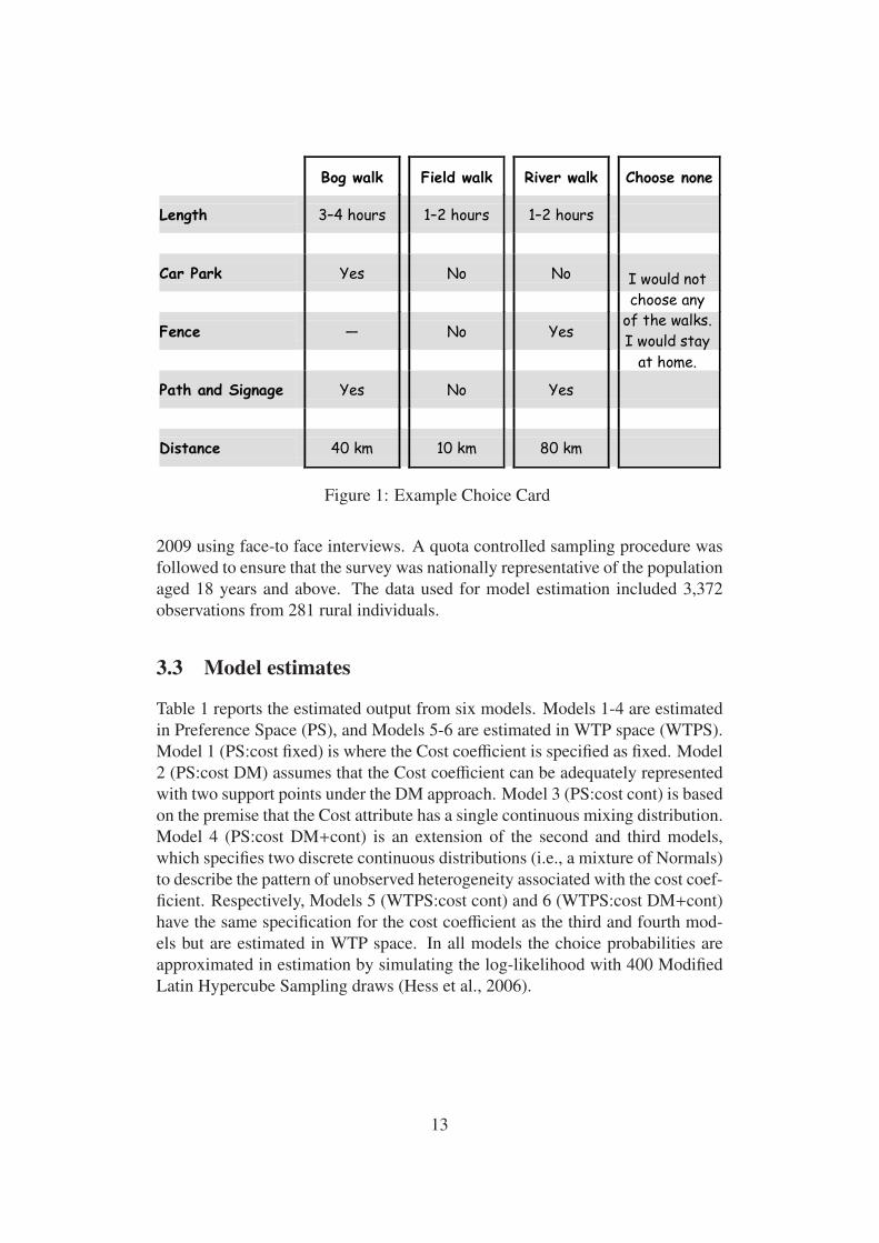
tomobile Association. An example of a choice task used for the DCE is given in
Figure 1.
In generating the choice scenarios this study adopted a Bayesian efficient de-
sign, based on the minimisation of the Db-error criterion (for a general overview
of efficient experimental design literature, see e.g., Scarpa and Rose, 2008, and
references cited therein). Our design comprised of a panel of twelve choice tasks.
For each task, respondents were asked to choose between a combination of the
experimentally designed alternatives and a stay at home option. When making
their choices, respondents were asked to consider only the information presented
in the choice task and to treat each task separately. Respondents were further re-
minded that distant trails would be more costly in terms of their time and money.
The survey was administered to a sample of Irish residents between 2008 and
12
��
�
��������� � ��������� � ��������� � ������������
��������
�
���������� � �������� � ���������
�
� � � � � � � � �
����������
�
� � � ��� � ��� � �
� � � � � � � � �
������
�
�� � ��� � � � � �
� � � � � � � � �
�����������������
�
� � � ��� � � � � �
� � � � � � � � �
���������
�
������ � ����� � ������ � �
�
�
�
������������
���� �����
����� �������
������������
������ ��
Figure 1: Example Choice Card
2009 using face-to face interviews. A quota controlled sampling procedure was
followed to ensure that the survey was nationally representative of the population
aged 18 years and above. The data used for model estimation included 3,372
observations from 281 rural individuals.
3.3 Model estimates
Table 1 reports the estimated output from six models. Models 1-4 are estimated
in Preference Space (PS), and Models 5-6 are estimated in WTP space (WTPS).
Model 1 (PS:cost fixed) is where the Cost coefficient is specified as fixed. Model
2 (PS:cost DM) assumes that the Cost coefficient can be adequately represented
with two support points under the DM approach. Model 3 (PS:cost cont) is based
on the premise that the Cost attribute has a single continuous mixing distribution.
Model 4 (PS:cost DM+cont) is an extension of the second and third models,
which specifies two discrete continuous distributions (i.e., a mixture of Normals)
to describe the pattern of unobserved heterogeneity associated with the cost coef-
ficient. Respectively, Models 5 (WTPS:cost cont) and 6 (WTPS:cost DM+cont)
have the same specification for the cost coefficient as the third and fourth mod-
els but are estimated in WTP space. In all models the choice probabilities are
approximated in estimation by simulating the log-likelihood with 400 Modified
Latin Hypercube Sampling draws (Hess et al., 2006).
13

Tab
le1
:M
od
elre
sult
s1
.P
S:c
ost
fixed
2.
PS
:co
stD
M3
.P
S:c
ost
con
t.4
.P
S:c
ost
DM+
con
t5
.W
TP
S:c
ost
con
t.6
.W
TP
S:c
ost
DM+
con
t
est.
t-ra
t.es
t.t-
rat.
est.
t-ra
t.es
t.t-
rat.
est.
t-ra
t.es
t.t-
rat.
Co
st
µ1
-0.0
46
-23
.55
-0.0
18
-8.0
5-0
.12
7-1
5.2
0-0
.06
9-7
.80
-0.1
13
-15
.01
-0.0
15
-3.9
7
σ1
0.1
04
14
.61
0.0
34
3.9
10
.07
61
4.5
80
.01
12
.12
π1
1.0
00
fixed
0.6
21
17
.96
1.0
00
fixed
0.4
61
9.8
61
.00
0fi
xed
0.7
05
16
.27
µ2
-0.2
12
-14
.97
-0.4
14
-9.6
5-0
.21
3-1
1.0
0
σ2
0.1
65
8.8
40
.10
71
0.5
6
π2
0.3
79
11
.39
0.5
39
11
.52
0.2
95
6.7
7
Len
gth
µ-1
.21
6-1
0.4
3-1
.33
8-1
0.1
8-1
.25
5-1
0.5
2-1
.50
5-1
1.7
5
σ1
.49
31
2.0
81
.81
41
4.0
01
.63
01
3.4
11
.59
81
2.6
6
µw
-12
.64
3-8
.52
-10
.67
1-9
.33
σw
15
.74
48
.93
11
.14
59
.89
Car
Par
k
µ0
.14
31
.88
0.2
98
3.6
00
.29
93
.73
0.2
94
3.4
8
σ0
.69
96
.99
0.6
86
5.8
80
.67
16
.29
0.7
47
6.1
2
µw
2.2
80
3.2
82
.16
73
.99
σw
4.2
19
4.3
52
.40
74
.08
Fen
ce
µ0
.20
92
.43
0.2
08
2.1
40
.24
92
.64
0.2
07
2.0
1
σ0
.30
31
.63
0.4
86
1.9
90
.34
82
.39
0.6
27
4.4
7
µw
1.7
67
2.1
06
0.9
49
1.3
9
σw
2.9
02
1.4
65
3.1
23
2.9
4
Pat
h
µ0
.47
46
.12
0.4
87
5.7
70
.51
76
.53
0.4
99
5.8
8
σ0
.57
54
.69
0.5
65
4.1
00
.38
32
.39
0.4
37
2.6
1
µw
3.4
44
.41
72
.38
64
.06
σw
4.3
72
3.5
30
3.3
55
3.3
6
Hil
lµ
0.8
88
6.2
71
.72
11
1.4
31
.64
71
1.2
02
.06
51
3.1
1
µw
9.3
26
7.0
92
7.2
77
.62
Bo
gµ
0.4
34
3.1
31
.11
17
.17
1.1
57
8.2
11
.44
49
.04
µw
8.2
11
6.8
96
.57
07
.31
Fie
ldµ
0.6
47
5.7
21
.49
19
.12
1.4
17
9.1
21
.82
41
1.0
0
µw
9.5
83
7.6
98
.20
08
.99
Riv
erµ
1.3
23
9.7
32
.32
21
4.4
02
.18
31
4.8
42
.69
41
6.1
0
µw
15
.47
21
1.6
21
1.4
13
10
.91
η(H
ill/
Bo
g)
σε
0.8
81
7.3
40
.93
47
.90
0.6
05
5.2
80
.80
46
.19
0.6
98
5.3
10
.83
65
.94
η(H
ill/
Fie
ld)
σε
0.9
87
7.9
21
.00
48
.84
1.0
36
8.9
60
.86
76
.18
1.1
01
8.7
61
.05
68
.01
η(H
ill/
Riv
er)
σε
1.0
37
8.5
80
.88
56
.84
1.0
48
8.6
21
.04
17
.88
1.2
85
11
.56
1.2
88
10
.71
η(B
og/F
ield
)σε
0.8
76
6.0
20
.83
86
.42
0.8
87
6.8
90
.91
27
.01
0.7
59
4.8
20
.73
84
η(B
og/R
iver
)σε
0.7
75
6.2
11
.00
18
.56
0.7
33
4.6
10
.90
57
.42
0.7
07
4.5
91
.10
77
.53
η(F
ield/R
iver
)σε
0.6
82
4.0
90
.84
16
.24
0.8
63
8.1
90
.81
46
.66
0.8
64
6.9
40
.87
66
.99
L(
β̂)
-3,3
76
.14
-3,0
58
.17
-3,1
03
.70
-3,0
11
.99
-3,1
72
.40
-3,1
24
.89
k1
92
22
02
52
02
4
Pse
ud
oR
20
.25
90
.32
40
.31
50
.33
40
.30
10
.30
9
BIC
69
06
.62
20
62
95
.06
37
63
69
.87
12
62
27
.06
75
65
07
.26
72
64
44
.75
43
AIC
67
90
.28
00
61
60
.35
20
62
47
.40
60
60
73
.98
60
63
84
.80
20
62
97
.79
60
3A
IC6
80
9.2
80
06
18
2.3
52
06
26
7.4
06
06
09
8.9
86
06
40
4.8
02
06
32
1.7
96
0
crA
IC6
79
5.0
42
86
16
7.6
06
56
25
2.9
22
46
08
4.4
79
36
39
0.3
18
46
30
7.1
20
6
µan
dσ
are
use
dre
spec
tivel
yto
rep
rese
nt
the
mea
nan
dst
and
ard
dev
iati
on
of
the
ran
do
mco
effici
ents
,aw
sub
scri
pt
ind
icat
esth
eval
ues
for
the
WT
Psp
ace
mo
del
s.π
isu
sed
tod
eno
teth
ep
rob
abil
itie
s
asso
ciat
edw
ith
the
mas
sp
oin
tsfo
rm
od
els
that
incl
ud
ed
iscr
ete
mix
ture
s.L
(
β̂)
den
ote
sth
elo
g-l
ikel
iho
od
val
ue
for
each
mo
del
.k
isth
en
um
ber
of
par
amet
ers.
Pse
ud
oR
2re
pre
sen
tsa
mo
del
fit
crit
erio
n.
Th
eB
IC,A
IC3
AIC
and
crA
ICre
pre
sen
tin
form
atio
ncr
iter
iad
evel
op
edb
yH
urv
ich
and
Tsa
i(1
98
9)
that
pen
alis
efo
rth
en
um
ber
of
par
amet
ers
esti
mat
ed(f
or
am
ore
in-d
epth
dis
cuss
ion
of
the
crit
eria
,se
e.g
.,H
yn
eset
al.,
20
08
).
14

Turning our attention first to the non-cost attributes in model 1 (PS:cost fixed),
the mean coefficient for Length, which is a dummy variable for longer walks4,
is negative, suggesting the general preference is for walks of a shorter duration.
Nevertheless, the retrieved coefficient of variation for the Length attribute is rela-
tively large, implying that a share of respondents do prefer taking walks over two
hours duration. This is not surprising as individuals are likely to differ in their
fitness levels and general preferences for engaging in farmland walks. The mean
coefficient for the Car Park attribute is positive, albeit only significant at the ten
percent level. However, the standard deviation is significant, indicating some re-
spondents do have a preference for car park facilities while another proportion
do not. This potentially suggests that a sizeable proportion of respondents may
dislike having a gravel car park near a walking trail because they may associate
it with issues of crowding at the walking sites or they may prefer more naturally
developed walking trails. A similar result is obtained for the Fence attribute.
This verifies the feedback from the focus group discussions, where some partici-
pants considered a fence would provide safety from livestock, whilst others felt a
fence would restrict their walking experience. As indicated by the positive mean
coefficient for Path, the majority of respondents prefer walking trails that are
paved. Relative to the stay at home option, all the alternative specific constants
are positive and significant—implying that respondents’ have a general prefer-
ence for participating in a farmland walk versus staying at home. Based on the
estimated coefficients, the most preferred walk type is River walks and the least
is Bog walks, with Hill and Field walks ranking in-between. The error compo-
nents between the walk alternatives are all significant suggesting that correlation
and substitution exists between the walks. The fixed cost coefficient is negative
and significant as expected.
Model 2 (PS:cost DM) specifies the cost coefficient to take two discrete val-
ues. This leads to a large improvement in model fit (an increase of 318 log-
likelihood units at the expense of 3 additional parameters), which provides strong
evidence against the use of a fixed cost coefficient and its implied equal marginal
sensitivity to cost across individuals. The model specification partitions respon-
dents into two distinct groups, based on the cost coefficient. The first group,
representing approximately 62 per cent of the sample are quite insensitive to cost
(as the discrete distribution lies in the negative domain but is close to zero), with
the second group estimated with a high sensitivity to cost (highlighted by its fur-
ther distance from zero). For the first group this low sensitivity to cost might
reflect the fact that some respondents are not strongly opposed to engaging in
walking trails that have a higher travel cost. The low sensitivity group may in-
clude respondents who have not attended to the cost attribute (which in this study
represents distance), which explains why their cost coefficient is estimated very
close to zero. Within the DCE literature, the issue of attribute non-attendance
4The attribute levels representing walks of between 2-3 hours and 3-4 hours in Length were
combined as their estimated coefficients were not statistically different
15

has been given considerable attention (e.g., Hensher and Rose, 2009; Campbell
et al., 2011; Scarpa et al., 2010, 2009), with some studies highlighting how cost
can often be the most ignored attribute (Scarpa et al., 2009). While we do not ex-
plicitly accommodate non-attendance in estimation, given the growing literature,
we suspect that our low sensitivity includes respondents who have not attended
to cost as well as respondents’ who have attended to cost (or distance) but were
not highly sensitive to it. Additionally, recent studies have shown that scale dif-
ferences may occur within and between discrete groups (Magidson and Vermunt,
2008; Boeri et al., 2011; Campbell et al., 2011). For instance, as noted by Camp-
bell et al. (2011), each discrete point may be comprised of a subset of respon-
dents, while having the same preferences, differ in their level of uncertainty and
hence variance leading to different scale factors. Furthermore, Boeri et al. (2011)
has shown how scale differences can emerge between discrete classes within the
latent class modelling framework. The signs and significance of the non-attribute
coefficients are similar to the first model, except the mean coefficient represent-
ing the car park attribute is significant.
In the third model we specify the cost coefficient to follow a single continuous
distribution. As can be seen from Table 1 this is estimated with fewer parame-
ters compared to when we specify cost with two discrete points. However the
BIC and AIC criteria suggest that the model represents a worse fit compared to
the previous specification. Additionally, the coefficient of variation for the Cost
coefficient is relatively high under this specification suggesting a share of the
distribution is within the positive domain. This could reflect a share of respon-
dents who are either relatively insensitive to cost or may not have attended to the
distance attribute within the CE. However it could also, in part, be an artefact of
using a single continuous Normal distribution to represent the heterogeneity of
the population with respect to cost.
In Model 4 (PS:cost DM+cont) the Cost attribute is specified with a mix-
ture of distributions. We assume two discrete mean coefficient values each with
an associated probability representing the discrete approach taken for Model 2
(PS:cost DM). The approach also allows additional heterogeneity within the two
subgroups specified. The approach relaxes the assumption that every respondent
lies on the same distribution with respect to Cost. This model assumes a fur-
ther improvement in model fit. As reflected by the Pseudo R2, the BIC and AIC
criteria this improvement is found even after penalising for the additional param-
eters. There is a lower share of respondents (π = 0.461) estimated to belong
to the low cost sensitivity group compared to the share predicted by the second
model (π = 0.531). Unlike Model 2 (PS:cost DM), which assumes homogeneity
within the subgroups, we find strong evidence of heterogeneity with respect to
cost, as both the standard deviations’ are highly significant in this model. The
remaining parameters are estimated with similar significance and magnitudes as
in the previous models. However, we note that the coefficients of variations tend
to be of a smaller magnitude, suggesting that for this dataset at least, allowing
16

for additional heterogeneity with respect to cost leads to lower variation with
respect to the non-cost attributes. This result implies that some of the variation
with respect to the cost attribute was potentially being captured by the non-cost
attributes, which may impact on subsequent policy decisions.
Our final two models presented in Table 1 are estimated in WTP space. To
reduce the number of models, we only present the results from two WTP space
specifications. Model 5 (WTPS:cost cont) assumes a single continuous distribu-
tion for the Cost coefficient. The mean of this distribution is found to be of a sim-
ilar magnitude as Model 6 (PS:cost DM+cont) , but as signified by the relative
standard deviation, the degree of heterogeneity is somewhat smaller. A useful
feature of WTP space models is the derivation of WT P directly. As can be seen,
the mean WT P estimates for all parameters are significantly different from zero.
The non-Cost attributes also have significant standard deviations. In terms of
welfare associated with the non-cost attribute, most disutility is associated with
longer length walks. For the remaining attributes, the mean WT P for path and
signage is largest, followed by car park. For the fence attribute there is substan-
tial welfare heterogeneity. Quite a large proportion of individuals are estimated
to have both positive and negative WT P estimates for the fence attribute.
In the final model we specify a mixture of distributions to represent the het-
erogeneity associated with the Cost attribute. The mean estimates and standard
deviations are all found to be significant. The results for the cost coefficient are
somewhat different to those obtained under model 4 (PS:cost DM+cont). Under
Model 6 (WTPS:cost DM+cont), the majority of respondents (π = 0.705) are
associated with a relatively low valued cost coefficient (which is similar to the
result attained in Model 2). The mean WT P estimates retrieved from this model
are similar to those attained under the previous WTP specification (albeit with
quite a lower estimated mean WT P for the length attribute) but the standard de-
viations are relatively smaller. The WTP space models achieve better fits over the
first model but they do not perform better than the remaining preference space
models. This is similar to the results presented by (e.g., Train and Weeks, 2005).
3.4 Implications for welfare estimation
Figure 2 illustrates the impact of the different distributional assumptions for the
cost coefficient on the retrieved unconditional WT P estimates for two of the non-
cost attributes. The distributions are estimated through simulation (see e.g. Hen-
sher and Greene 2003, for an in-depth discussion) where 10,000 draws are taken
from the distribution of the non-cost and cost attributes, and the ratio of the non-
cost to cost attribute is calculated for each draw. The ratios are draws from the
distribution of WT P (Daly et al., Forthcoming). Under the first model (PS:cost
fixed), since Cost is the denominator and is fixed, the distribution of WT P takes
on the same distribution as the non-Cost coefficient, thus facilitating straight-
17

Len
gth
DensityM
odel
1
−1
00
−5
00
50
0.0000.020
Len
gth
Density
Model
2
−1
00
−5
00
50
0.000.03
Len
gth
Density
Model
3
−1
00
−5
00
50
0.000.06
Len
gth
Density
Model
4
−1
00
−5
00
50
0.000.08
Len
gth
Density
Model
5
−1
00
−5
00
50
0.000.04
Len
gth
Density
Model
6
−1
00
−5
00
50
0.000.04
(a)
(Unco
ndit
ional
)W
TP
dis
trib
uti
ons
for
Len
gth
Pat
h
Density
Model
1
−4
0−
20
02
04
0
0.0000.015
Pat
h
Density
Model
2
−4
0−
20
02
04
0
0.000.03
Pat
h
Density
Model
3
−4
0−
20
02
04
0
0.000.06
Pat
h
Density
Model
4
−4
0−
20
02
04
0
0.000.10
Pat
h
Density
Model
5
−4
0−
20
02
04
0
0.000.03
Pat
h
Density
Model
6
−4
0−
20
02
04
00.000.04
(b)
(Unco
ndit
ional
)W
TP
dis
trib
uti
ons
for
Pat
han
dS
ignag
e
Fig
ure
2:
Co
mp
aris
on
of
(un
con
dit
ion
al)
WT
Pd
istr
ibu
tio
ns
18

forward WT P estimation. However, as shown, in the case of all attributes, this
model produces distributions that are relatively more dispersed than those esti-
mated when heterogeneity in the cost coefficient is accommodated. There is a
general reduction in the degree of WT P dispersion as one moves to the fourth
model which uses a mixture of distributions approach.
We present median WT P in Table 2 as Balcome et al. (2009) note that me-
dian values are more stable than mean estimates for RPL models estimated in
preference space. Across all models, the median WT P estimate to avoid a longer
length walk, is relatively large compared to the utility associated with the other
attributes. Therefore in general, individuals have a strong preference for farm-
land walks that are relatively shorter in duration. This likely reflects the walking
habits of the Irish population, where not that many individuals engage in walks
that are over two hours duration. For the remaining attributes, the WT P for path
and signage is largest, followed by car park. The relatively lower WT P estimate
for the fence attribute likely reflects the substantial heterogeneity associated with
this attribute under the models. In general the models suggested that a proportion
of individuals had both positive WT P for a fence and a proportion who are WT P
to avoid a farmland trail that is fenced-off from livestock. Although not unex-
pected, this has some implications in terms of the implementation of farmland
walking trails as it suggests, a mixture of trails is necessary that differ in terms
of their features.
Table 2: Comparison of median WTP per trip estimates (AC)
Model Length Long Car Park Fence Path
1.PS: Cost fixed -29.31 3.65 5.18 11.61
2.PS:cost DM -15.29 3.4 2.25 5.23
3.PS:cost cont -6.91 1.59 1.37 2.92
4.PS: cost DM+cont -5.87 1.19 0.82 1.92
5.WTPS:cost cont -12.77 2.33 1.78 3.51
6.WTPS: cost DM+cont -10.82 2.21 0.91 2.34
As evident from Table 2 the distributional assumptions associated with the cost
attribute has an impact on the retrieved WT P estimates. Taking the longer length
attribute as an example, there is a huge reduction in the median WT P estimate
between the first and the fourth model specification. It must be noted that while
lower welfare estimates are retrieved from Model 4(PS: cost DM+cont), they are
similar to the estimates from the other models with random cost coefficients. In
particular, the estimates do not differ substantially between the third and fourth
model specification in preference space. For the WTP space models slightly
lower welfare estimates are retrieved from the Model 6 (WTPS: cost DM+cont)
compared to Model 5 (WTPS:cost cont). Overall, our best model fit was asso-
ciated with the preference space model using the mixtures distribution for cost.
19

Generally the lower estimates retrieved from this model, compared to the other
specifications that included discrete mixtures, most likely reflects the lower es-
timated share of respondents associated with a mass point closer to zero in this
model. We also find that using a fixed cost coefficient is both associated with
a poorer model fit and larger retrieved welfare estimates. Hence, we find little
support for this approach either empirically, based on the model fit, or from a
policy perspective, based on its associated welfare estimates. However, whilst
the retrieved median estimates are larger under this model, we do not know what
the true underlying WT P values are to speculate on which model specification
provides the closest estimates to the true values. We must acknowledge, also that
our WT P estimates may reflect the higher bound in term of welfare estimates be-
cause it is based on the assumption that the person answering the survey would
bear all the out of pocket travel expenses. In Ireland, previous studies have found
that between 38 and 50 percent of people indicate that they walk alone for long
and short walks respectively. In the case of short and long walks (up to 4 hours)
approximately 38 and 45 percent of respondents indicate that the walk with one
other companion only. Of the people who walk with one other companion ap-
proximately 60 percent walk with another family member or partner. As a result
we would expect that in the majority of cases, costs are most likely borne either
directly by the person answering the survey or within their household. Neverthe-
less, it could be likely that some respondents answering the choice experiments
would assume that they would not have to bear the full costs themselves of travel-
ling to the walks and as a result our estimates most likely reflect the upper bound
in terms of individual WT P. As noted by a reviewer the low cost sensitivity
groups that we observed may reflect individuals who assumed that they would
not have to bear the full costs of travelling to the sites.
4 Conclusion
Since the value of farmland as a recreational resource is potentially high, a careful
assessment of the benefits from this resource is essential when deciding on the al-
ternative uses of farmland. Determining the preferences of potential recreational
users’ is useful from a policy perspective as it allows managers, landowners and
other stakeholders with the necessary information to provide suitable amenities
at recreational sites. To this end, this paper explored preferences of Irish rural
residents for the provision of farmland walking trails in the Irish countryside.
In Ireland, property rights are such that recreational users do not currently have
the same access to the countryside as other European countries. As a result, a
stated preference study using the CE methodology was employed to elicit these
preferences.
A further objective of this paper was to compare alternative methods to ac-
commodate heterogeneity associated with the cost coefficient in a RPL model of
20

recreational site-choice. We compared a number of models assuming either a dis-
crete, continuous or mixture of discrete and continuous distributions, to represent
cost heterogeneity. Our reference model assumed a fixed cost coefficient, and the
remaining models allowed for different random specifications for cost. We also
compared the distributional implications for the cost coefficient in preference
and WTP Space. We found that the preference space model which enabled addi-
tional cost heterogeneity using a combination of discrete and continuous mixing
distributions provided the best fit for the data. Beyond this, we also found that
this model specification was associated with the lowest WT P distributions for
the non-cost attributes explored in this study. However, in general, the policy
implications arising from the models, where the cost coefficient was specified as
random, did not differ substantially from each other. In general we found little
support empirically for fixing the cost coefficient in RPL models, which echoes
findings by Balcome et al. (2009).
In choosing which random distribution to use for the cost coefficient a number
of points are noteworthy. First, the DM approach (without including the continu-
ous distribution) may be useful in situations where the analyst wishes to constrain
all cost heterogeneity to be in the negative preference domain. An advantage of
this approach is that the analyst is not required to specify a particular distribution
for the random heterogeneity and it makes welfare estimation more straightfor-
ward. On the other hand the mixtures of distribution approach may be useful
when the analyst does not have strong a priori expectations, for either cost or
non-cost attributes, regarding the shape of the distributions. In particular the ad-
ditional parameters associated with the mixtures approach means that it is more
capable of representing a range of potential distributions. While our focus on the
cost coefficient may be somewhat arbitrary it mirrors a growing interest within
the literature in using multi-modality distributions to represent unobserved het-
erogeneity (e.g., Fosgerau and Hess, 2009; Fosgerau and Bierlaire, 2007; Scarpa
et al., 2008; Hensher and Greene, 2013). Campbell et al (2010) show how the
mixtures of distributions approach can be extended to a number of attribute coef-
ficients in their preference space models. However, we must acknowledge some
limitations of the approach. In the preference space models, while we noticed
a lower mass at the extremes of the WT P distribution we did not find that the
mixtures of distributions approach overcomes the problem of obtaining extreme
WT P estimates at the tails of the distribution. Additionally, where the distribu-
tion traverses zero, as in the case of the normal distribution for cost, the WT P
distribution may not have well-defined moments in preference space (Daly et al.,
Forthcoming). We did not observe these problems with the mixtures approach in
WTP space. An avenue for further research is to examine the applicability of the
approach to other distributions. In the case of the cost coefficient, for instance,
a mixture of distributions that ensure that the distribution is bounded below zero
may be advantageous to ensure the distribution of WT P has well-defined mo-
ments in preference space. In the case of the WTP space model specification
21

bounding the distribution for cost is likely to be advantageous because it ensures
that the scale parameter is bounded below zero to ensure finite variance. We
explored the possibility of using the mixtures approach with the Johnson SB dis-
tribution, which can be bounded. However, we found a mixtures of distributions
did not work well for the Johnson SB distribution, which is most likely due to the
number of parameters required to estimate this distribution. Furthermore, while
we do not include covariates without our model specifications, we note that their
inclusion could enhance the generalizability of the approach we have used.
Notwithstanding the fact that we found significant heterogeneity associated
with each attribute, a few general policy observations should be noted. First,
countryside residents showed a much stronger preference for walking trails that
are shorter in length. This has implications for the development of these trails
because it implies that only smaller tracks of farmland may be needed to develop
the trails and hence, less cost should be associated with their development. In
terms of the other attributes, generally, car-parking facilities and path and sig-
nage facilities were favoured by the majority of respondents. Approximately
half of respondents favoured trails that were fenced off from livestock. This
suggests that a mixture of trail types may be warranted, with different infrastruc-
tural features. In general, Irish rural residents showed the highest preference for
river farmland walking trails. Given that rivers are spread throughout the Irish
countryside this result suggested that substantial supply side potential may ex-
ist to develop these trails, if farmers are willing to participate in such farmland
walkway schemes. While the other walk types, namely hill, field and bog walks
were not as strongly preferred as river walks, Irish countryside residents did also
show a positive preference for these walks. These results confirm that significant
demand exists for more extensive development of the Irish countryside for recre-
ational pursuits. Providing access to the countryside for recreation would bring
Ireland in line with the majority of other European countries.
22

References
Balcome, K., Chalak, A. and Fraser., I. (2009). Model selection for the mixed
logit model with Bayesian estimation, Journal of Environmental Economics
and Management 57: 226–237.
Boeri, M. (2011). Advances in Stated Preference Methods: Discrete and Con-
tinuous Mixing Distributions in Logit Models for Representing Variance and
Taste Heterogeneity, PhD thesis, Queen’s University Belfast.
Boeri, M., Doherty, E., Campbell, D. and Longo, A. (2011). Accommodating
taste and variance heterogeneity in discrete choice, International Choice Mod-
elling Conference, Leeds UK.
Buckley, C., Hynes, S. and van Rensburg., T. (2008). Public access for walking in
the Irish countryside? can supply be improved?, Tearmann - The Irish Journal
of Agri-Environmental Research, 6: 1–14.
Buckley, C., Hynes, S., van Rensburg, T. and Doherty., E. (2009). Walking
in the Irish countryside - landowners preferences and attitudes to improved
public access provision, Journal of Environmental Planning and Management
52: 1053–1070.
Buckley, C., van Rensburg, T. and Hynes, S. (2008). What are the financial
returns to agriculture from a common property resource? a case study of Irish
commonage, Journal of Farm Management 13: 311–324.
Buckley, C., van Rensburg, T. and Hynes, S. (2009). Recreational demand for
farm commonage in Ireland: a contingent valuation assessment, Land Use
Policy 26: 846–854.
Bujosa, A., Riera, A. and Hicks, R. (2010). Combining discrete and continuous
representations of preference heterogeneity: a latent class approach, Environ-
mental and Resource Economics 47: 477–493.
Campbell, D. (2007). Willingness to pay for rural landscape improvements:
combining mixed logit and random-effects models, Journal of Agricultural
Economics 58(3): 467–483.
Campbell, D. and Boeri, M. and Longo, A. (2010). Accommodating hetero-
geneity for reducing traffic problems: A “mixed” latent class approach. Paper
presented at the European Transport Conference, Glasgow, 10-13th October.
Campbell, D., Hensher, D. A. and Scarpa, R. (2011). Non-attendance to at-
tributes in environmental choice analysis: a latent class specification, Journal
of Environmental Planning and Management 54: 1061–1076.
23

Carlsson, F., Frykblom, P. and Lagerkvist, C. J. (2007). Consumer benefits of
labels and bans on GM foods—choice experiments with Swedish consumers,
American Journal of Agricultural Economics 89: 152–161.
Colombo, S., Angus, A., Morris, J., Parsons, D., M.Brawn, K.Stacey and Han-
ley., N. (2009). A comparison of citizen and expert preferences using an
attribute-based approach to choice, Ecological Economics 68: 2834–2841.
Colombo, S., Calatrava-Requena, J. and Hanley, N. (2007). Testing choice ex-
periment for benefit transfer with preference heterogeneity, American Journal
of Agricultural Economics 89(1): 135–151.
Curtis, J. and Williams, J. (2005). A national survey of recreational walking in
Ireland, Technical report, Economic and Social Research Institute, Dublin.
Daly, A., Hess, S. and Train, K. (Forthcoming). Assuring finite moments for
willingness to pay in random coefficient models, Transportation.
Failte (2009). Hiking and walking facts 2008, Technical report, Failte Ireland.
Fiebig, D., Keane, M., Louviere, J. and Wasi, N. (2010). The generalized multi-
nomial logit model: accounting for scale and coefficient heterogeneity, Mar-
keting Science 29: 393–421.
Fitzpatrick and Associates (2005). The economic value of trails and forest recre-
ation in the Republic of Ireland, Technical report, Coillte Publications, Wick-
low.
Fleischer, A. and Tsur, Y. (2000). Measuring the recreational value of agricultural
landscape, European Review of Agricultural Economics 27(3): 385–398.
Fosgerau, M. and Bierlaire, M. (2007). A practical test for the choice of mix-
ing distribution in discrete choice models, Transportation Research Part B
41: 784–794.
Fosgerau, M. and Hess, S. (2009). A comparison of methods for represent-
ing random taste heterogeneity in discrete choice models, European Transport
42: 1–25.
Hensher, D. A. and Greene, W. H. (2003). The mixed logit model: the state of
practice, Transportation 30: 133–176.
Hensher, D. A. and Greene, W. H. (2013). Revealing additional dimensions
of preference heterogeneity in a latent class mixed multinomial logit model,
Applied Economics 45: 1897–1902.
24

Hensher, D. and Greene, W. (2011). Valuation of travel time savings in WTP and
preference space in the presence of taste and scale heterogeneity, Journal of
Transport Economics and Policy 45: 505–525.
Hensher, D. and Rose, J. (2009). Simplifying choice through attribute preser-
vation or non-attendance: implications for willingness to pay, Transportation
Research Part E: Logistics and Transportation Review 45: 583–90.
Hess, S., Bierlaire, M. and Polak, J. W. (2007). A systematic comparison of
continuous and discrete mixture models, European Transport 37: 35–61.
Hess, S., Train, K. E. and Polak, J. W. (2006). On the use of a modified latin
hypercube sampling (MLHS) method in the estimation of a mixed logit model
for vehicle choice, Transportation Research Part B 40: 147–163.
Hurvich, C. and Tsai, C. (1989). Model selection for extended quasi-likelihood
models in small samples, Biometrika 76: 297–307.
Hynes, S., Buckley, C. and van Rensburg, T. (2007). Recreational pursuits on
marginal farm land: a discrete-choice model of Irish farm commonage recre-
ation, Economic and Social Review 38: 63–84.
Hynes, S., Campbell, D. and Howley, P. (2011). A holistic versus an attribute
based approach to agri-environment policy evaluation: do welfare estimates
differ?, Journal of Agricultural Economics 62: 305–329.
Hynes, S., Hanley, N. and Scarpa, R. (2008). Effects on welfare measures of
alternative means of accounting for preference heterogeneity in recreational
demand models, American Journal of Agricultural Economics 90: 1011:1027.
Lyall, A. (2000). Land Law in Ireland, Dublin: Oak Tree Press.
Magidson, J. and Vermunt, J. (2008). Removing the scale factor confound in
multinomial logit choice model to obtain better estimates of preferences, In
Proceedings of the Sawtooth Software Conference, Sawtooth Software.
Morey, E. and Rossmann, K. G. (2008). Calculating,with income effects, the
compensating variation for a state change, Environmental and Resource Eco-
nomics 39(2): 83?90.
Provencher, B. and Bishop, R. C. (2004). Does accounting for preference het-
erogeneity improve the forecasting of a random utility model? a case study,
Journal of Environmental Economics and Management 48: 793–810.
Scarpa, R., Campbell, D. and Hutchinson, W.G. (2007). Benefit estimates for
landscape improvements: sequential Bayesian design and respondents’ ratio-
nality in a choice experiment Land Economics 83: 617–634.
25

Scarpa, R., Ferrini, S. and Willis, K. G. (2005). Performance of error component
models for status-quo effects in choice experiments, In (Scarpa, R and Alberini,
A, eds): Applications of Simulation Methods in Environmental and Resource
Economics, Springer, Dordrecht.
Scarpa, R., Gilbride, T., Campbell, D. and Hensher, D. (2009). Modelling at-
tribute non-attendance in choice experiment for rural landscape preservation,
European Review of Agricultural Economics pp. 1–24.
Scarpa, R. and Rose, J. (2008). Design efficiency for non-market valuation with
choice modelling: how to measure it, what to report and why, The Australian
Journal of Agricultural Economics 52: 253–282.
Scarpa, R., Thiene, M. and D.A., Hensher. (2010). Monitoring choice task at-
tribute attendance in nonmarket valuation of multiple park management ser-
vices, Land Economics 86: 817–839.
Scarpa, R., Thiene, M. and Maragon, F. (2008). Using flexible taste distributions
to value collective reputation for environmentally friendly product methods,
Canadian Journal of Agricultural Economics 56: 145–162.
Scarpa, R., Thiene, M. and Train., K. E. (2008). Utility in willingness to pay
space: a tool to address confounding random scale effects in destination choice
to the Alps, American Journal of Agricultural Economics 90: 994–1010.
Sonnier, G., Ainslie, A. and Otter, T. (2007). Heterogeneity distributions of
willingness-to-pay in choice models, Quantitative Marketing and Economics
5: 313–331.
Thiene, M. and Scarpa, R. (2009). Deriving and testing efficient estimates of
WTP distributions in destination choice models, Environment and Resource
Economics 44: 379–395.
Torres, C., Hanley, N. and Riera., A. (2011). How wrong can you be? im-
plications of incorrect utility function specification for welfare measurement,
Journal of Environmental Economics and Management 62: 111–121.
Train, K. E. and Weeks, M. (2005). Discrete choice models in preference space
and willing-to-pay space, In (Scarpa, R and Alberini, A, eds):Applications
of Simulation Methods in Environmental and Resource Economics, Springer,
Dordrecht.
Wasi, N. and Carson, R. (2011). The influence of rebate programs on the de-
mand for water heaters: the case of New South Wales. Paper presented at the
55th Australian Agricultural and Resource Economics Society National Con-
ference, 8-11th February, 2011.
26

