University of Calgary

PRISM: University of Calgary's Digital Repository

Graduate Studies The Vault: Electronic Theses and Dissertations

2013-11-14

The Roles of the Normal Mechanical Properties of

Articular Cartilage in the Contact Mechanics of the

Human Knee Joint: a Finite Element Approach

Dabiri, Yaghoub

Dabiri, Y. (2013). The Roles of the Normal Mechanical Properties of Articular Cartilage in the

Contact Mechanics of the Human Knee Joint: a Finite Element Approach (Unpublished doctoral

thesis). University of Calgary, Calgary, AB. doi:10.11575/PRISM/28370

http://hdl.handle.net/11023/1161

doctoral thesis

University of Calgary graduate students retain copyright ownership and moral rights for their

thesis. You may use this material in any way that is permitted by the Copyright Act or through

licensing that has been assigned to the document. For uses that are not allowable under

copyright legislation or licensing, you are required to seek permission.

Downloaded from PRISM: https://prism.ucalgary.ca

UNIVERSITY OF CALGARY

The Roles of the Normal Mechanical Properties of Articular Cartilage in the Contact Mechanics

of the Human Knee Joint: a Finite Element Approach

by

Yaghoub Dabiri

A THESIS

SUBMITTED TO THE FACULTY OF GRADUATE STUDIES

IN PARTIAL FULFILMENT OF THE REQUIREMENTS FOR THE

DEGREE OF DOCTOR OF PHILOSOPHY

DEPARTMENT OF MECHANICAL AND MANUFACTURING ENGINERING

CALGARY, ALBERTA

NOVEMBER, 2013

© Yaghoub Dabiri 2013

Abstract

In spite of numerous research devoted to the study of the mechanical behaviour of

cartilage, few of them considered fluid pressure in an anatomically accurate knee joint model.

Including the fluid phase as a cartilage constituent, this thesis investigated the mechanics of

human knee joint. The main hypothesis of this thesis was that the depth-wise integrity of the

structure of cartilage has an important role in its mechanical performance especially its fluid

pressurization. The roles of depth-dependent properties, local degenerations and defects on the

knee joint mechanics were modeled. Moreover, the effect of individual muscle forces on the

knee joint mechanics was investigated.

In one of our studies, four models including healthy and degenerated cartilage with local

OA progressed from the superficial, to the middle and deep zones were compared. In another

study, the effects of depth-wise progression of a local cartilage defect on the knee contact

mechanics were investigated. A model with individual muscle forces was compared with a

model without muscle forces to examine the effects of muscle forces.

The normal cartilage produced higher surface fluid pressure under a given compression.

The lack of structural integrity, as happened in local cartilage degeneration, resulted in reduced

fluid pressure in the degenerated zone as well as at the cartilage-bone interface. Cartilage defects,

on the other hand, had more complex effects on knee joint mechanics. While a local superficial

defect reduced pressure in the remaining affected cartilage, a defect advanced to the middle zone

increased fluid pressure. Regarding effects of muscle forces, the knee mechanics was noticeably

affected when muscles were included. Contact pressure, for instance, was significantly increased

in a model with muscle forces compared to a model without muscle forces.

ii

The results were in line with previous experimental and computational studies that

reported the importance of the structural integrity and depth-dependent properties of cartilage.

Integrating fluid pressure, complex three-dimensional geometry, depth-dependent properties,

individual muscle forces, and a more realistic treatment of free surface fluid pressure, this project

aimed to better understanding of human knee joint mechanics. Results may contribute to better

understanding of osteoarthritis as well as the design of artificial cartilage.

iii

Acknowledgements

First of all, I would like to give a special thank you to my family for their patience and support.

Among different people who helped me in this project, my supervisor, Dr. LePing Li, had a

crucial role, and I greatly thank him for his efforts during my program. I would like to thank the

supervisory committee members Dr. Steven Boyd and Dr. Simon Park for their comments, and

examiners Dr. Lidan You and Dr. Elena Di Martino for their efforts in reviewing my thesis and

for their questions and comments during the examination. I would like to express my gratitude to

my colleagues Dr. Mojtaba Kazemi and Mr. Sahand Ahsanizadeh for their precious technical

help as well as their friendship. I also would like to thank the previous member of our research

group Mr. Bill Gu for his help when I started the project. I owe a warm thank you to Mr. Stephen

Cull for his assistance in language and friendship. I would like to give thank you to Dr. Doug

Philips and Dr. Hartmut Schmider for their crucial supports with the computational facilities. I

would like to extend my thanks to Dr. Tannin Schmidt, and Dr. Frank Cheng for acting as the

examiners in my candidacy examination.

iv

Dedication

To my parents

v

Table of Contents

ABSTRACT........................................................................................................................II

ACKNOWLEDGEMENTS.............................................................................................. IV

LIST OF TABLES..........................................................................................................VIII

LIST OF FIGURES AND ILLUSTRATIONS................................................................. IX

LIST OF SYMBOLS, ABBREVIATIONS AND NOMENCLATURE .......................... XI

CHAPTER ONE: INTRODUCTION................................................................................12 1.1 Prevalence of Knee Osteoarthritis ...............................................................................12 1.2 Importance of the Mechanical Modeling.....................................................................13 1.3 Thesis Overview ..........................................................................................................16 1.4 Statement of Contribution............................................................................................17

CHAPTER TWO: BACKGROUND.................................................................................18 2.1 Knee Anatomy .............................................................................................................18 2.2 Cartilaginous Tissues ...................................................................................................20

2.2.1 Swelling of Cartilage ............................................................................................22 2.2.2 Macrostructure of Articular Cartilage and Meniscus ...........................................23 2.2.3 Cartilage Mechanical Tests...................................................................................25

2.3 Cartilage Mechanical Models ......................................................................................26 2.3.1 Single-Phase Models.............................................................................................27 2.3.2 Biphasic Models ...................................................................................................27 2.3.3 Fiber Reinforced Models ......................................................................................28

2.4 Knee Joint Numerical Models .....................................................................................28

CHAPTER THREE: INFLUENCES OF THE DEPTH-DEPENDENT MATERIAL INHOMOGENEITY OF ARTICULAR CARTILAGE ON THE FLUID PRESSURIZATION IN THE HUMAN KNEE ................................................................32 3.1 Abstract ........................................................................................................................32 3.2 Introduction..................................................................................................................33 3.3 Methods........................................................................................................................36 3.4 Results..........................................................................................................................41 3.5 Discussion ....................................................................................................................51 3.6 References....................................................................................................................57

CHAPTER FOUR: ALTERED KNEE JOINT MECHANICS IN SIMPLE COMPRESSION ASSOCIATED WITH EARLY CARTILAGE DEGENERATION ....64 4.1 Abstract ........................................................................................................................64 4.2 Introduction..................................................................................................................65 4.3 Methods........................................................................................................................68 4.4 Results..........................................................................................................................73 4.5 Discussion ....................................................................................................................82 4.6 References....................................................................................................................89

vi

CHAPTER FIVE: LOAD BEARING CHARACTERISTICS OF THE KNEE JOINT DETERIORATES WITH THE DEFECT DEPTH OF ARTICULAR CARTILAGE......97 5.1 Abstract ........................................................................................................................97 5.2 Introduction..................................................................................................................98 5.3 Methods......................................................................................................................100 5.4 Results........................................................................................................................103 5.5 Discussion ..................................................................................................................114 5.6 References..................................................................................................................118

CHAPTER SIX: A PROTOCOL TO INCLUDE INDIVIDUAL MUSCLE FORCES IN AN ANATOMICALLY ACCURATE MODEL OF THE HUMAN KNEE JOINT......125 6.1 The Coordinates of Origin and Insertion Points of Muscles......................................126 6.2 The Forces of Muscles ...............................................................................................132

6.2.1 Enforcing Angles ................................................................................................132 6.2.2 Enforcing Moments ............................................................................................134

6.3 The Optimization Process ..........................................................................................134 6.4 Inclusion of Muscle Forces in the ABAQUS Model .................................................136 6.5 MATLAB M-files......................................................................................................138 6.6 Results........................................................................................................................139

CHAPTER SEVEN: FREE-SURFACE FLUID PRESSURE.........................................142 7.1 Subroutines ................................................................................................................143

7.1.1 FLOW Subroutine...............................................................................................143 7.1.2 URDFIL Subroutine ...........................................................................................145

7.2 Result File ..................................................................................................................148 7.3 Testing the algorithm .................................................................................................149 7.4 Application to the Anatomically Accurate Model .....................................................149

CHAPTER EIGHT: CONCLUSION ..............................................................................153 8.1 Summary....................................................................................................................153 8.2 Limitations .................................................................................................................154 8.3 Future Work ...............................................................................................................157

REFERENCES ................................................................................................................160

APPENDIX 1: THE MATLAB CODE DEVELOPED TO TEST THE FORTRAN CODE FOR ZERO FLUID PRESSURE BOUNDARY CONDITION......................................170

APPENDIX 2: THE FORTRAN CODE DEVELOPED TO IMPLEMENT THE ZERO FLUID PRESSURE FOR NON-CONTACTING SURFACES......................................171

APPENDIX 3: THE COPYRIGHT PERMISSION LETTER ........................................177

JOURNAL AND CONFERENCE PAPERS AND ABSTRACTS.................................182

vii

List of Tables

Table (3-1). Material properties for all tissues used in the inhomogeneous model ..........39

Table (3-2). Material properties for the femoral cartilage in the homogeneous model ....41

Table (4-1). Material properties for the normal tissues ....................................................73

Table (5-1). Ten cases investigated in the present study ................................................103

Table (6-1). The coordinates of origin point of muscles in the knee joint.......................129

Table (6-2). The coordinates of insertion point of muscles in the knee joint ..................130

Table (6-3). The coordinates of the intersection point of muscles line of action ............131

Table (6-4). The moment arm and maximum isometric force of three muscles used in this project (yang et al., 2010, o’connor 1993, kellis and baltzopoulos 1999).......................136

viii

List of Figures and Illustrations

Fig. 2.1. The components of the knee joint........................................................................20

Fig. 2.2. The structure of pgs. ............................................................................................22

Fig. 2.3. The depth-dependent structure of cartilage. ........................................................24

Fig. 2.4. Cartilage tests ......................................................................................................25

Fig 3.1. Total reaction force in the knee joint as a function of time..................................42

Fig. 3.2. Variation of fluid pressure and compressive stress (mpa) along the depth of the femoral cartilage ................................................................................................................43

Fig. 3.3. First principal stress or strain along the depth of the femoral cartilage ..............45

Fig. 3.4. Fluid pressure in the sagittal plane of the femoral cartilage that is cut through the medial condyle ...................................................................................................................46

Fig. 3.5. Fluid pressure in the coronal plane of the femoral cartilage that is cut through the medial condyle ...................................................................................................................47

Fig. 3.6. Maximum fluid pressure in a given layer of elements ........................................48

Fig. 3.7. Fluid pressure at 100s as predicted by the inhomogeneous model......................49

Fig. 3.8. Fluid pressure at 100s as predicted by the homogeneous model .........................50

Fig. 4.1. Finite element model of the tibiofemoral joint, showing the distal femur ..........69

Fig. 4.2. Fluid pressure (mpa) at the normalized depth of 1/16 (superficial layer) ...........75

Fig. 4.3. Fluid pressure (mpa) at the normalized depth of 13/16 (deep layer)...................76

Fig. 4.4. Variation of fluid pressure along the depth of the femoral cartilage...................77

Fig. 4.5. Fluid pressure (mpa) in a sagittal plane of the medial condyle. ..........................78

Fig. 4.6. Fluid pressure (mpa) in a coronal plane of the medial condyle...........................79

Fig. 4.7. Lateral strain along the depth of the femoral cartilage........................................80

Fig. 4.8. First principal strain at the normalized depth of 15/16 (deep layer) ...................81

Fig. 4.9. Shear strains at the normalized depth of 15/16 (deep layer) ...............................82

Fig. 5.1. Surface fluid pressure in the femoral cartilage at 500µm compression ............104

Fig. 5.2. Surface fluid pressure in the femoral cartilage during late relaxation...............105

Fig. 5.3. Fluid pressure in the layer of normalized depth of 1/16 at 500µm ...................107

Fig. 5.4. Fluid pressure in a sagittal plane of the femoral cartilage at 500µm.................108

Fig. 5.5. Reaction force in the knee as a function of time. ..............................................110

Fig. 5.6. Surface fluid pressure in the femoral cartilage at 500µm compression ............111

ix

Fig. 5.7. Shear strain in the deepest cartilage layer .........................................................112

Fig. 5.8. Surface fluid pressure in the femoral cartilage at 387.76n ................................113

Fig. 5.9. Reaction force in the knee as a function of time during the loading phase for the cases of creep and stress relaxation .................................................................................114

Fig. 6.1. Seven coordinate systems are shown in this figure. the origin and insertion coordinates are calculated in these frames.......................................................................127

Fig. 6.2: Inclusion of individual muscle forceS...............................................................138

Fig. 6.3: Contact pressure in the femoral cartilage with (a) and without (b) muscles for approximately 40% of the gait cycle. ..............................................................................141

Fig. 7-1: This algorithm is used to distinguish if an integration point is in contact. .......147

Fig. 7-2: A simple model was used to test the algorithm for finding the closest node to an integration point within the master surface......................................................................149

Fig. 7-3: Surface fluid pressure at the femoral cartilage..................................................151

Fig. 7-4: Surface fluid pressure at the femoral cartilage when no boundary condition was enforced for the free surfaces (@3s)................................................................................152

x

List of Symbols, Abbreviations and Nomenclature

Symbol Definition

𝝈𝝈 Total stress 𝝈𝝈𝑒𝑒𝑒𝑒𝑒𝑒 Solid stress, or effective stress −𝝈𝝈𝑒𝑒𝑓𝑓 Component of stress due to fluid pressure 𝑝𝑝 pore pressure 𝝈𝝈𝑚𝑚 Stress in the nonfibrillar matrix 𝝈𝝈𝑒𝑒 Stress in the fibrillar matrix 𝜆𝜆, 𝜇𝜇 Lamé constants 𝑒𝑒 Volumetric strain 𝜺𝜺 Strain 𝐸𝐸𝑥𝑥,𝑦𝑦,𝑧𝑧 Young’s modulus in x, y or z direction 𝐸𝐸𝑚𝑚 Young’s modulus of the nonfibrillar matrix 𝜐𝜐 Poisson’s ratio of the nonfibrillar matrix 𝑘𝑘𝑥𝑥,𝑦𝑦,𝑧𝑧 Permeability in x, y or z direction 𝜐𝜐𝑥𝑥 Fluid velocity in the x direction 𝑝𝑝𝑒𝑒,𝑥𝑥 X component of fluid pressure gradient 𝜏𝜏Rzx Shear strain parallel to cartilage-bone interface and in x direction 𝜏𝜏Rzy Shear strain parallel to cartilage-bone interface and in y direction 𝛾𝛾zx Shear stress parallel to cartilage-bone interface and in x direction 𝛾𝛾zy Shear stress parallel to cartilage-bone interface and in y direction ��𝜃 Angular acceleration at hip, knee or ankle 𝐻𝐻,𝐾𝐾,𝐴𝐴

��𝜃 Angular velocity at hip, knee or ankle 𝐻𝐻,𝐾𝐾,𝐴𝐴

𝑀𝑀𝐻𝐻,𝐾𝐾,𝐴𝐴 Muscle moment at hip, knee or ankle 𝐽𝐽 Performance criterion 𝑎𝑎𝑚𝑚 Activation of muscle number m 𝐹𝐹𝑚𝑚 Force of muscle number m 𝐹𝐹𝑚𝑚0 Maximum isometric force of the muscle number m 𝑓𝑓 Fluid velocity in the direction of outward normal to cartilage surface 𝑘𝑘0 Seepage coefficient 𝛾𝛾𝑤𝑤 specific weight 𝑐𝑐 Characteristic length of an element

POR Fluid pressure (in ABAQUS) S First principal stress (in ABAQUS)

xi

Chapter One: Introduction

1.1 Prevalence of Knee Osteoarthritis

The knee joint is a complex joint of the human body. Daily activities like walking,

jumping, stair ascent and descent require knee joint function. Research that aim to

reproduce the functions of a biological knee with an artificial one encountered numerous

difficulties such as control, strength, cosmetics, and weight of the joint (Dabiri et al.,

2013, Martinez-Villalpando and Herr 2009, Sup et al., 2008). The knee joint is vulnerable

to disease and injury.

In 2003, knee problems were the main reason for visiting an orthopaedic surgeon

(American Academy of Orthopaedic Surgeons (AAOS), 2007). Knee injuries have been

reported to happen in many sport activities (Hashemi et al., 2011, Cheatham and Johnson,

2010, Larson and Grana, 1993, AAOS, 2007). Among the diseases that might occur at

this joint, the following are examples: osteoarthritis, varus, valgus, tear of ligaments of

knee, injuries to meniscus, and fractures in the joint (Cailliet, 1992).

Arthritis is a common disease of the knee joint. This word stems from Greek

“arthron” and “itis”. The first part means joint and the second part means inflammation.

There are different kinds of arthritis. Osteoarthritis is the most common form of arthritis.

In osteoarthritis, cartilage is gradually degenerated, and eventually leads to bone to bone

contact. This bone to bone contact makes the joint painful. In rheumatic arthritis, another

kind of arthritis, the joint is painful and swollen. Infectious arthritis is another kind of

12

arthritis whereby an infection happens in the joint. This infectious arthritis makes the

joint painful as well (Nordqvist, 2009).

Arthritis is the leading cause of disability in the United States (Centers for

Disease Control and Prevention, 2012), and is reported as one of the major causes of

work limitation (Stoddard et al., 1998). The prevalence of arthritis is higher in the older

population. In the United States, almost 80% of people above 65 years of age suffer from

arthritis (Lawrence et al., 1989, Bagge and Brooks, 1995, Manek and Lane, 2000).

Osteoarthritis (OA) of the joints is the most prevalent cause of disability within the

elderly (Manheimer et al., 2007, Peat et al., 2001, Centers for Disease Control and

Prevention, 2001). Among different joints, the knee has the highest incidence

(Manheimer et al., 2007, Felson and Zhang, 1998, Oliveria et al., 1995). OA is

recognized as a disease with noticeable effects on the sociological, the economical and

the well-being aspects of life (Saarakkala et al., 2010). The prevalence and related costs

of knee osteoarthritis are expected to rise during the next 25 years (Manheimer et al.,

2007, Lethbridge-Cejku et al., 2004).

1.2 Importance of the Mechanical Modeling

OA is divided into two categories: primary OA, and secondary OA. The exact cause of

primary OA is not known; however, it develops as a result of cartilage wear, and is

relevant to how long the joint is used. On the other hand, secondary OA develops as a

results of abnormal conditions like injury, and congenital factors (Tsahakis et al., 1993,

13

Mow and Ratcliffe, 1997). In any case, mechanical loading is the leading parameter in

OA initiation and progression.

While OA is a process including mechanical and biological phenomena, it is

defined as the degeneration of a joint caused primarily by mechanical loading (Radin,

1990 adopted from Pauwels, 1976). In primary OA, the cartilage lesion initiates at a

location which is not routinely under load. An initial lesion develops into other load

bearing areas. A lesion at a load bearing area might further progress into deep cartilage

provided the underlying bone has hardened (Radin, 1990). The progression of lesion into

deep layers, finally leads to cartilage loss and bone to bone contact. In secondary OA, the

initiation of OA might happen from cartilage-bone interface (Atkinson and Haut, 1995).

In this case, the mechanical loading causes microfractures at cartilage-bone interface,

which will develop to further cartilage degeneration.

Therefore, the knowledge about the mechanical behavior of the knee joint is an

essential element in understanding the pathogenesis of osteoarthritis. However, the

complexities involved in the structure and function of the joint make the mechanics of the

joint complicated. The mechanical behavior of the knee joint could be assessed in an

experimental approach or in a mathematical modeling approach. Using an experimental

approach is not always feasible due to some limitations pertaining to ethical issues or

difficulties in practical procedures.

Unlike experimental approaches, mathematical approaches are not limited by

ethical issues. However, some simplifying assumptions have to be made in order to

model the knee joint. The more realistic a mathematical model is, the more reliable

14

results will be. Mathematical models could be divided into two subcategories: analytical

and computational models. The former is capable of producing accurate results for

models that are highly simplified. Computational models, however, could overcome

some of the complexities of modeling the biological joint, and avoid some simplifications

made in an analytical model.

This project used the Finite Element Method (FEM) to study the mechanical

behavior of the knee joint. Three hypotheses investigated in this project were: (1) surface

fluid pressure at the cartilage is enhanced by depth-dependent properties; (2) a local

cartilage degeneration in a high load-bearing area in the medial femoral condyle causes

fluid pressure reduction in the cartilage, and a deeper degeneration is associated with a

higher reduction in fluid pressure; (3) a local cartilage defect in a high load-bearing area

in the medial femoral condyle causes fluid pressure reduction in the cartilage, and a

deeper defect is associated with a higher reduction in fluid pressure. The importance of

individual muscle forces in the contact mechanics was modeled as well. Moreover, free

surface fluid pressure boundary condition was improved compared to previous models.

The commercial software ABAQUS (Simulia Inc., Providence, RI, USA) was used to

implement FEM. By eliminating some limitations which were applied to the previous

studies, this project advances the knowledge of knee joint mechanics. The results could

have implications in prevention and treatment of OA. Designing artificial articular

cartilage using the tissue engineering techniques is another application as suggested in the

literature (Ateshian and Hung, 2005).

15

1.3 Thesis Overview

This is a paper-based thesis. Chapters 3, 4, and 5 are published, accepted journal papers,

or submitted manuscript.

Chapter 3:

Dabiri Y, Li LP. Influences of the depth-dependent material inhomogeneity of articular

cartilage on the fluid pressurization in the human knee. Medical Engineering & Physics

2013; 35(11), 1591-1598.1

Chapter 4:

Dabiri Y, Li LP. Altered knee joint mechanics in simple compression associated with

early cartilage degeneration. Computational and Mathematical Methods in Medicine

2013; 2013:1-11, http://dx.doi.org/10.1155/2013/862903.2

Chapter 5:

Dabiri Y, Li LP. Load Bearing Characteristics of the Knee Joint Deteriorates with the

Defect Depth of Articular Cartilage, Submitted.

Chapters 1 and 2 provide the motivations and background of this work. Chapters

3, 4, and 5 present the mechanics of normal and diseased cartilage with the progression of

OA. Considering a normal model, chapter 3 presents the importance of the depth-

dependent structure and integrity of articular cartilage. The models developed in Chapter

3 (including Table 3-1) were based on models developed by our research group

previously (Gu, 2010). Targeting the early stages of OA, chapter 4 discusses the effects

1 The relevant copyright permission license number from Elsevier is 3207701479466 (Appendix 3). 2 Copyright permission was not required by the journal.

16

of depth-wise progression of degeneration on the mechanical behavior of cartilage.

Considering advanced stages of OA, chapter 5 studies cartilage defects representing the

more severe stages of OA.

Chapters 6 and 7 aim to remove two simplifications in the anatomically accurate

models developed in our research group. Chapter 6 describes a method to consider

individual muscle forces. As a suggestion for future work, the resultant knee joint model

from Chapter 6 can be used to analyse daily living activities such as gait. Chapter 7

introduces a methodology that automatically enforces the free-surface pore pressure

boundary conditions during the solution, based on contact conditions. The fixed free-

surface pore pressure condition used in Chapters 3-5 is only suitable for small knee

compression as will be discussed in Chapter 7. Chapter 8 summarizes the thesis and

explains possible future directions. The references provided in Chapters 4, 5, and 6 are

not repeated in the final “Reference” list that provides the references cited in Chapters 1,

2, 6, 7 and 8.

1.4 Statement of Contribution

The author of this thesis and his supervisor are the authors of the papers used to compose

this thesis (Chapters 3, 4, and 5), and they did the pertaining research work including

development of the computational models, simulations, analysing the results, and writing

the papers.

17

Chapter Two: Background

2.1 Knee Anatomy

There are three classifications for the joints in the human body, namely, synovial

(diarthrodial), cartilaginous (amphiarthroses) and fibrous (synarthroses) joints. Knee and

hip joints are examples of synovial joint which enjoy more mobility compared to the two

other classifications. Examples of cartilaginous and fibrous joints are intervertebral and

skull joints, respectively (Mow and Ateshian, 1997).

The knee joint is one of the biggest joints in the body. This joint is composed of

bones, muscles, ligaments, cartilaginous and other soft tissues (Grana and Larson, 1993).

There are four ligaments in the knee joint that stabilize and control its motion: 1- ACL:

Anterior Cruciate Ligament, 2- PCL: Posterior Cruciate Ligament, 3- MCL: Medical

Collateral Ligament, and 4- LCL: Lateral Collateral Ligament.

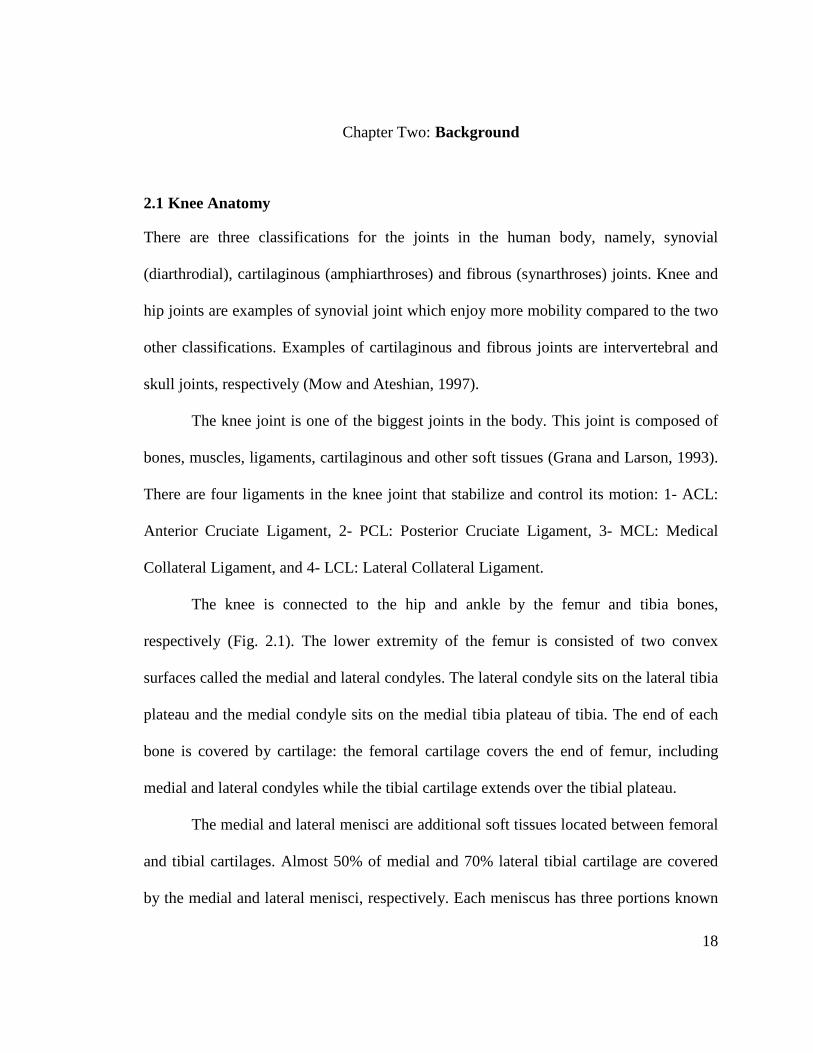
The knee is connected to the hip and ankle by the femur and tibia bones,

respectively (Fig. 2.1). The lower extremity of the femur is consisted of two convex

surfaces called the medial and lateral condyles. The lateral condyle sits on the lateral tibia

plateau and the medial condyle sits on the medial tibia plateau of tibia. The end of each

bone is covered by cartilage: the femoral cartilage covers the end of femur, including

medial and lateral condyles while the tibial cartilage extends over the tibial plateau.

The medial and lateral menisci are additional soft tissues located between femoral

and tibial cartilages. Almost 50% of medial and 70% lateral tibial cartilage are covered

by the medial and lateral menisci, respectively. Each meniscus has three portions known

18

as body, anterior and posterior horns. The medial meniscus is larger, and has a more open

side toward the intercondylar notch. The anterior and posterior horns of medial meniscus

are attached to the tibial plateau. The outer edge of medial meniscus is connected to the

joint capsule. The shape of the lateral meniscus is close to a circle. The anterior horn of

the lateral meniscus is connected to the anterior horn of the medial meniscus through the

transverse ligament. The posterior horn of the lateral meniscus is attached to the posterior

tibia and also has connections with the medial femoral condyle and the popliteus (Rath

and Richmond, 2000, Fox, 2007).

The knee joint is surrounded by a fibrous tissue called the joint capsule lined by

the synovial membrane (synovium). The space within the joint, formed by cartilages and

synovium, is called the joint cavity which is filled with synovial fluid. The synovial fluid,

which is secreted by synovium, plays an important role in lubrication and nourishment of

the joint (Mow and Ateshian, 1997, Nordqvist, 2009).

The third bone in the knee joint is the patella or knee cap. It is located at the

anterior side of the joint and as its primarily function, patella facilitates knee extension.

The fibula is another bone attached proximally to the tibia, and distally to the ankle joint.

At full extension, the femur and tibia define joint mechanics, whereas the patella and

fibula do not play an important role in load support. These components of the knee joint

are depicted in Fig. 2.1.

19

Fig. 2.1. The components of the knee joint (http://en.wikipedia.org/wiki/File:Knee_diagram.svg)

2.2 Cartilaginous Tissues

Cartilage is divided into three groups: hyaline cartilage, elastic cartilage and

fibrocartilage. Articular cartilage is the most common type of hyaline cartilage. Articular

cartilage can be found at the end of long bones in articulating joints like the femoral and

tibial cartilages. The external auditory canals is an example of elastic cartilage. The

cartilage in the intervertebral joints and knee meniscus are examples of fibrocartilages

(Mow and Ratcliffe, 1997).

The tensile properties of cartilage are mainly governed by collagens. The collagen

type in articular cartilage is mainly type II, and the collagen type in meniscus is mainly

20

type I. The diameter of collagens in meniscus is larger than in articular cartilage (Mow

and Ratcliffe, 1997).

The cartilaginous tissues (articular cartilage and meniscus) are composed of two

main phases: a liquid phase and a solid phase. The solid phase is mainly composed of

proteoglycans (PGs), collagens, and chondrocytes. The liquid phase is composed of water

and electrolytes.

The compressive stiffness of articular cartilage is mainly due to proteoglycans

(PGs) (Kempson et al., 1970). PGs are composed of a core protein to which the

glycosaminoglycans (GAGs), including keratine and chondroitin sulfate, are attached.

Proteoglycans could aggregate to hyaluronic acids and, as shown in Fig. 2.2, form a

bottle-brush like structure (Mansour, 2004). The GAG chains contain negative charges,

and produce the cartilage fixed charge density or FCD (Mow and Ratcliffe, 1997). As a

result of the PGs’ negative charge, the fluid pressure within cartilage will be higher than

environmental fluid pressure, and their difference will produce Donnan osmotic pressure

(Mow and Ratcliffe, 1997).

PGs constitute almost 30% of cartilage dry weight (Mansour, 2004), and 5-10%

of its wet weight (Mow and Ratcliffe, 1997). The concentration of PGs varies with depth.

At the surface they have the lowest concentration (~15% dry weight), and their highest

concentration (~25% dry weight) is at the middle region (Mow and Ratcliffe, 1997,

Athanasiou et al., 2010).

21

Fig. 2.2. The structure of PGs.

The FCD applies a swelling pressure within cartilage. This swelling pressure

helps cartilage to support higher loads (Mow and Ratcliffe, 1997). Therefore, the

negative charges in the PGs also contribute to the compressive stiffness of articular

cartilage (Mansour, 2004).

2.2.1 Swelling of Cartilage

The repulsion of identical electrical charges of PGs and the higher fluid pressure caused

by them results in cartilage swelling (Mow and Ratcliffe, 1997). As mentioned before,

the identical charges within PGs produce a fluid pressure which is higher than

environmental fluid pressure. Also, the identical charges produce repulsion forces that

contribute to cartilage swelling. These forces play a role in bearing the applied load.

22

2.2.2 Macrostructure of Articular Cartilage and Meniscus

The extracellular matrix (ECM) of articular cartilage is a network of collagen fibers

embedded in a gel built from PGs. Therefore, cartilage can be considered as a fiber

reinforced composite solid (Mizrahi et al., 1986, Mow and Ratcliffe, 1997).

The structure of cartilage varies with depth. As shown in Fig. 2.3, the tissue is

often divided into three zones. The superficial zone comprises ~10-20% of cartilage

thickness. In this zone, the collagen fibers are oriented parallel to the surface according to

the split-lines. The concentration of collagens in this zone is the highest, while the

concentration of PGs is the lowest. The middle (transitional) zone comprises ~40-60% of

cartilage thickness. The collagen fibers are dispersed randomly in this zone. The

concentration of PGs is the highest, and the concentration of collagen fibers is lower

compared to the surface zone. The deep zone comprises ~30% of cartilage tissue in which

the fibers are perpendicular to the cartilage tide mark. The subchondral and cancellous

bones are located below the deep zone and tide mark (Mow and Ratcliffe, 1997). The

mechanical properties of cartilage also vary along the depth, which will be explained in

section 3.2.

23

Fig. 2.3. The depth-dependent structure of cartilage.

As mentioned earlier, similar to articular cartilage, meniscus is also comprised of

the nonfibrillar matrix, fluid, and fibers. The fibers are mainly randomly oriented in the

surface zone of menisci. Almost 100 µm from the surface, within the two-thirds of the

peripheral region, the fibers are oriented circumferentially. These circumferential fibers

are grouped together by supporting radial fibers. In the inner regions, the fibers are

randomly oriented (Mow and Ratcliffe, 1997).

Articular cartilage is an inhomogeneous tissue. The properties of articular

cartilage are both site- and depth-dependent. Site-dependency implies the variation of the

properties of cartilage with location at a specific depth, whereas depth-dependency is

associated with the alteration of the properties in a depth-wise manner.

24

2.2.3 Cartilage Mechanical Tests

In experimental studies of cartilage, four main test configurations can be found (Hasler et

al., 1999, Knecht et al., 2006, Korhonen et al., 2002): unconfined compression, confined

compression, indentation (Fig. 2.4) and tensile testing.

(a) Load (b) Load

Permeable Piston Cartilage Sample Cartilage Impermeable Plates

Sample

Confining Chamber Fig. 2.4. Cartilage tests: (a) confined compression, (b) unconfined (c) Load compression, (c) indentation.

Indenter Cartilage

Subcondral Bone

In a confined setup, the fluid is not allowed to escape through the surrounding

wall, although it can escape through the load-applying piston. The stress-strain results

from confined compression tests can be used to calculate the aggregate modulus and

permeability. For this purpose, based on the biphasic theory (Mow et al., 1980),

compressive stress and applied strain are fitted to the experimental data (Schinagl et al.,

1997, Soltz and Ateshian, 1998). The Young’s modulus can also be calculated from the

confined compression experiment (Korhonen et al., 2002).

25

In unconfined compression, the cartilage sample is under an impermeable plate,

and fluid flow can exude from the lateral sides. This setup can be used to measure the

dynamic modulus of cartilage under a sinusoidal (Park et al., 2004) or instantaneous

deformation step (Saarakkala et al., 2003). After equilibrium is reached, the static

Young’s modulus and Poisson ratio can be calculated.

The indentation test is another experiment used to calculate the mechanical

properties of cartilage. The indentation test can be used to calculate the Young's modulus

and the shear modulus of the cartilage assuming the cartilage is a linear elastic solid

material (Hayes et al., 1972). Compared with the confined and unconfined compression

tests, the advantage of using an indentation test is to keep the integrity of the tissue in the

testing region.

The tensile specimen of cartilage is similar to those discussed in the Mechanics of

Materials, except the cross-section can only be rectangular. Dumbbell shape specimens

are often prepared.

2.3 Cartilage Mechanical Models

Cartilage is generally poromechanical, viscoelastic, anisotropic, and heterogeneous. Its

behavior is strain and strain rate dependent, and its responses differ in tension and

compression (Taylor and Miller, 2006).

Analytical methods could be used to solve the governing equations when the

material model and geometry are sufficiently simplified. Numerical methods, however,

are often used to extract the mechanical parameters from measured data (Carter and

26

Wong, 2003 adopted from Hughes, 1987). For complex testing geometries and realistic

material models, only numerical methods are capable of solving the problem.

2.3.1 Single-Phase Models

Single-phase models assume cartilage as an incompressible or nearly incompressible

solid material (Carter and Wong, 2003). These models can be appropriate for loading

conditions where the fluid flow is not significant such as in short term static loading or

moderate to high frequency cyclic loading (Carter and Wong, 2003).

2.3.2 Biphasic Models

The other approach to model cartilage acknowledges the presence of fluid inside the

tissue. When the fluid exudation is significant, the single phase models fail to predict the

response of articular cartilage, which is time dependent. The poroelastic or consolidation

(Biot, 1941) and biphasic or mixture (Mow et al., 1980) models consider the time-

dependent response produced by the fluid pressurization (Hasler et al., 1999, Taylor and

Miller, 2006, Carter and Wong, 2003). The consolidation approach assumes the material

as a porous solid saturated with fluid. The biphasic approach assumes the material as a

continuum mixture of the solid and fluid parts. Basically, these are two different methods,

but for an incompressible material they are equivalent (Levenston et al., 1998). At each

point of cartilage, the total stress is the sum of the effective stress and the fluid pressure:

𝝈𝝈 = 𝝈𝝈𝑓𝑓𝑓𝑓 + 𝝈𝝈𝑒𝑒𝑓𝑓𝑓𝑓 (2-1)

27

Where σ, σfland σeff are the total stress, fluid stress (the negative of the pore pressure),

and effective stress (or stress in the solid), respectively. Using pore pressure p

𝝈𝝈 = −𝑝𝑝𝐈𝐈 + 𝝈𝝈𝑒𝑒𝑓𝑓𝑓𝑓 (2-2)

2.3.3 Fiber Reinforced Models

In the fiber reinforced model, the collagen fibers are included in the modeling. The tissue

is assumed to be composed of a nonfibrillar matrix and collagen network. The

nonfibrillar matrix supports compression, some tension, and shear and the fibrillar matrix

supports only tension. In mathematical form:

𝝈𝝈𝑒𝑒𝑓𝑓𝑓𝑓 = 𝝈𝝈𝑚𝑚 + 𝝈𝝈𝑓𝑓 (2-3)

Where 𝝈𝝈𝑒𝑒𝑒𝑒𝑒𝑒 is the effective stress in both matrices, 𝝈𝝈𝑚𝑚 is the stress supported by

nonfibrillar matrix, and 𝝈𝝈𝑒𝑒 is the stress in the fibrillar matrix which is zero under

compression. In the fibril-reinforced models, the time-dependent response is accounted

for by the fluid flow and intrinsic viscoelasticity of the collagen network (Li et al., 1999;

Li and Herzog, 2004). The fibril-reinforced poro-viscoelastic models also consider the

intrinsic viscoelasticity of the nonfibrillar (PG) matrix (Wilson et al., 2004).

2.4 Knee Joint Numerical Models

Cartilage models with standard simplified geometry fail to explain important features

inherent to the complex three-dimensional geometry of cartilaginous tissues. Regarding

the knee joint, femoral cartilage, tibial cartilages, and menisci not only are in contact

28

altogether but also they are attached to bones. The multiple contacts between

cartilaginous tissue and their attachments to the bones have important roles in the

mechanical behavior of both the whole knee joint and individual cartilaginous tissues.

For example, the femoral cartilage is in contact with menisci and tibial cartilages, and it

is bonded to the femur. The fluid flow and displacements at the contacting and the

cartilage-bone interface regions influence the mechanical behavior of femoral cartilage.

Those regions, however, are defined by the three-dimensional geometry of the femoral

cartilage as well as the tibial cartilages, the menisci, and the femur distal head. Moreover,

the orientations and locations of individual muscle forces can be defined in a model if the

three-dimensional geometry of the knee joint is considered.

Three-dimensional models have been developed to analyze the mechanical

behavior of the knee joint. They have followed different mathematical approaches to take

geometrical and material properties of the knee joint into consideration. Some studies

implemented more simplifying assumptions. The numerical solutions became more

dominant rather than exact analytical solutions as studies tried to model the knee joint

more realistically. The reader could compare a study by Blankevoort and colleagues and

another report by Bendjaballah and colleagues (Blankevoort et al., 1991, Bendjaballah et

al., 1995). In the former study the bone surfaces were approximated using polynomials

(continuous functions), but the latter study reconstructed bone surfaces from

computerized tomography data using segmented images. In addition, the former study

(Blankevoort et al., 1991) failed to consider cartilages as separate parts in the model but

considered their effect on the contact between bones whereas the latter study

29

(Bendjaballah et al., 1995) analyzed the model with cartilages as additional parts

discretized into finite elements.

Knee joint computational models could be validated using experimental data such

as contact pressure and deformations (Kazemi et al., 2013). For instance, the

patellofemoral contact pressure and area for different knee angles were reported in a

study (Powers et al., 1998), where the mean contact stress under an axial load at 0º knee

flexion angle was 0.62 MPa. The maximum contact pressure in the tibial cartilage was

reported to be 5.5 MPa in another study (Papaioannou et al., 2008). The reported data

depend on the conditions of the experiments including the magnitude of the load,

constraints, and knee joint angle.

Anatomically accurate three-dimensional (3D) models of the knee joint are

developed from imaging data (Kazemi et al., 2013). The geometry of our model was built

based on MRI. Software packages such as Mimics (Materialise, Leuven, Belgium), and

Rhinoceros (Seattle, WA, USA) were used to segment the images and reconstruct the 3D

geometry. The geometry was then meshed for finite element calculations using software

packages such as ABAQUS (Simulia, Providence, USA).

The work presented in this thesis could be considered as a progress in numerical

modeling of the knee joint. Several anatomically accurate finite element models have

been reported in the literature. Each study is based on simplifying assumptions such as

exclusion of fluid pressure, considering cartilaginous tissues as isotropic linear elastic

models, ignoring the depth-dependent properties, neglecting effects of a lesion depth on

the lesion progression, and ignoring the individual muscle forces (Bendjaballah et al.,

30

1995, Peña et al., 2005, Shirazi et al., 2008, Mononen et al., 2012). This project provides

a model where some of these limitations are removed.

31

Chapter Three: Influences of the Depth-dependent Material Inhomogeneity of Articular Cartilage on the Fluid Pressurization in the Human Knee3

3.1 Abstract

The material properties of articular cartilage are depth-dependent, i.e. they differ in the

superficial, middle and deep zones. The role of this depth-dependent material

inhomogeneity in the poromechanical response of the knee joint has not been investigated

with patient-specific joint modeling. In the present study, the depth-dependent and site-

specific material properties were incorporated in an anatomically accurate knee model

that consisted of the distal femur, femoral cartilage, menisci, tibial cartilage and proximal

tibia. The collagen fibers, proteoglycan matrix and fluid in articular cartilage and menisci

were considered as distinct constituents. The fluid pressurization in the knee was

determined with finite element analysis. The results demonstrated the influences of the

depth-dependent inhomogeneity on the fluid pressurization, compressive stress, first

principal stress and strain along the tissue depth. The depth-dependent inhomogeneity

enhanced the fluid support to loading in the superficial zone by raising the fluid pressure

and lowering the compressive effective stress at the same time. The depth-dependence

also reduced the tensile stress and strain at the cartilage–bone interface. The present 3D

modeling revealed a complex fluid pressurization and 3D stresses that depended on the

mechanical contact and relaxation time, which could not be predicted by existing 2D

3 This chapter contains a journal paper published on Medical Engineering and Physics. The relevant copyright permission license number from Elsevier is 3207701479466 (Appendix 3).

32

models from the literature. The greatest fluid pressure was observed in the medial

condyle, regardless of the depth-dependent inhomogeneity. The results indicated the roles

of the tissue inhomogeneity in reducing deep tissue fractures, protecting the superficial

tissue from excessive compressive stress and improving the lubrication in the joint.

KEYWORDS: Articular cartilage mechanics; Cartilage heterogeneity; Collagen fiber

orientation; Finite element analysis; Fluid pressure; Knee joint mechanics

3.2 Introduction

The major components of articular cartilage are collagen fibers, proteoglycans and

synovial fluid (Mow et al., 1980, Mow and Ratcliffe, 1997). The compressive and shear

stiffness of the tissue are governed by the proteoglycan matrix, while the tensile stiffness

is governed by the collagen fibers. The collagen network also greatly contributes to the

apparent compressive stiffness at fast loading through the fluid pressurization, which is

enhanced by fiber reinforcement (Mizrahi et al., 1986, Li et al., 2002). The fluid is also

responsible for the poromechanical behavior of the tissue (Mow et al., 1990): the fluid

pressure supports up to 90% of applied compressive loading (Ateshian and Hung, 2005),

which reduces to an insignificant level at equilibrium. The cartilaginous tissues are

commonly modeled as biphasic (Mow and Mansour, 1977, Mak et al., 1987).

The structure and properties of cartilage, e.g. fiber orientation and hydraulic

permeability, change along the depth of the tissue from the articular surface to the bone

interface (Maroudas and Bullough, 1968, Minns and Steven 1977). This change is

33

referred to as depth-dependent material inhomogeneity, or zonal differences. The

superficial zone is composed of fibers parallel to the articular surface, the fibers in the

middle zone are not oriented in a specific direction, and the fibers in the deep zone are

mainly perpendicular to the bone surface (Weiss et al., 1968, Minns and Steven 1977,

Jeffery et al., 1991). The importance of depth-dependent inhomogeneity has been the

subject of experimental and theoretical studies (Schinagl et al., 1997, Chen et al., 2001a,

Chen et al., 2001b, Mow and Guo, 2002, Julkunen et al., 2007, Federico and Herzog,

2008, Chegini and Ferguson 2010, Saarakkala et al., 2010,). These studies could be

categorized into (1) simplified geometries that pertain to standard testing such as

confined and unconfined compression tests (Schinagl et al., 1997), and (2) three-

dimensional anatomically accurate geometries (Shirazi et al., 2008).

Concerning the first category, previous studies reported the importance of depth-

dependence in the mechanical behavior of articular cartilage in unconfined compression

tests (Korhonen et al., 2008, Li et al., 2000, Li et al., 2002). The mechanical behavior of

cartilage with depth-dependent properties in confined compression was also investigated

simultaneously with unconfined compression (Wilson et al., 2004, Wilson et al, 2005). In

addition, it was reported that the alternation of permeability along the depth affected fluid

pressurization and the mechanical behavior of the tissue (Setton, et al., 1993).

The second category, three-dimensional models of human knee, has been

developed to study the mechanical behavior of the knee in normal and pathological

conditions (Bendjaballah et al., 1995, Périé and Hobatho., 1998, Peña et al., 2005, Peña et

al., 2008). Only two of the 3D models, however, have considered the material properties

34

in a depth-dependent manner. The first one was an elastic model without fluid pressure

(Shirazi et al., 2008). The second one modeled the fluid pressure and zonal dependent

fiber orientation to investigate the short-term load response (Mononen et al., 2012),

which is virtually elastic. The influence of the depth-dependence may not have been

adequately shown in these two studies because of two reasons. First, the mechanical

response of the tissue associated with the collagen network is more significant when

substantial fluid pressure is present (Mizrahi et al., 1986, Oloyede et al., 1992, Li et al.,

2002). Second, the poromechanical response was not investigated. A previous study

indicated more significant influence of fiber orientation during early relaxation (Li et al.,

2009).

Therefore, the objective of the present study was to determine what mechanical

parameters of articular cartilage in the knee were affected by the depth-dependent

material inhomogeneity. We were interested in fluid pressurization and dissipation in the

tissues. An MRI-based knee joint model was used for this purpose. The collagen fibers,

depth-dependent inhomogeneity, and fluid pressure were simultaneously considered for

the cartilaginous tissues. In order to understand the significance of the depth-dependence,

the results from the proposed model were compared with those obtained from a recently

published model that did not include the depth-dependence (Gu and Li, 2011). The

proposed model was otherwise the same as the published model: the fiber and fluid

phases were particularly considered in both models.

35

3.3 Methods

A recently published knee joint model (Gu and Li, 2011) was modified to include depth-

dependent material properties in the femoral cartilage. The proposed model will be

referred to as the inhomogeneous model, because both depth-dependent and site-specific

material properties were incorporated. For the convenience of discussion, the published

model will be referred to as the homogeneous model: it was homogeneous in the

direction of the tissue thickness, although the site-specific material properties were also

considered.

In the literature, the continuous variation of the depth-dependence is often

characterized with three distinct zones. The superficial, middle and deep zones contain,

respectively, 10%-20%, 40%-60% and almost 30% of the cartilage thickness (Mow et al.,

1992, Newman, 1998). For the simplicity of the present inhomogeneous modeling, the

three zones were taken to be approximately 25%, 50% and 25% of the cartilage

thickness. They were further meshed with 2, 4 and 2 layers of elements respectively.

Therefore, there were in total 8 layers of elements in the thickness direction. As the input

of the finite element analysis, the fibers in the superficial zone were assumed to be in

split-line directions (Below et al., 2002); the fibers in the middle zone were randomly

distributed along the three directions, and the fibers in the deep zone were oriented

perpendicular to the bone surface.

For the tibial cartilage, complete measurement data of fiber orientation were not

found from the literature, although split-lines in the submeniscal region were arranged in

a wheel-spoke pattern (Goodwin et al., 2004). Therefore, the mechanical properties were

36

assumed the same for all directions, i.e. no preferred fiber orientation was considered for

the tibial cartilage. For the meniscus, the fibers were incorporated primarily in the

circumferential and secondly in the radial directions (Fithian et al., 1990).

The constitutive behavior of the tissues is described by a fibril-reinforced model

previously published (Li et al., 2000). Some equations are included here for the

convenience of reading. The total stress in the tissue, which is the stress in the mixture, is

determined by the fluid pressure, p, and the effective stress of the solid matrix, σeff

σ = − pI σ+ eff (3-1)

where the effective stress consists of the effective stress of the orthotropic fibrillar matrix,

σ f , and the effective stress of the isotropic nonfibrillar matrix defined by the Lamé

constants λ and µ

eff fσ = λeI + 2µε σ+ (3-2)

where e is the volumetric strain and ε is the strain. The fibrillar matrix mimics the

collagen network, while the nonfibrillar matrix mimics the proteoglycan matrix. As a first

approximation, the fibrillar stress is neglected if the tissue is in compression in the fiber

direction. The tensile stress in the fibrillar matrix is determined by (Li et al., 2009)

dσ f = E f dε (3-3)x x x

where Exf is the fibrillar modulus in the x-direction, which aligns in the direction of

fibers or primary fibers. For the case of small fibrillar strains,

37

E f = E0 + Eε ε (3-4)x x x x

where Ex 0 and Ex

ε are direction- and depth-dependent constants. Replacing x with y and

z, respectively, will derive the corresponding equations for the transverse directions.

Obviously, this formula will not be valid when the tensile strain is large. Fortunately,

when cartilage is compressed from the articular surface, the lateral tensile strain is only a

fraction of the compressive strain. Therefore, this simple formula can approximate

moderate compressions.

The Lamé constants λ and µ in Eq. (3-2) can be replaced by the Young’s modulus

and Poisson’s ratio, Em and νm , of the nonfibrillar matrix. For the inhomogeneous

model, the two parameters for the femoral cartilage were approximated as linear

functions of the tissue depth z

(3-5)Em = E m (1+αE z h) ,νm =ν m (1+ αν z h)

νwhere Em and m are respectively the Young’s modulus and Poisson’s ratio at the

articular surface; h is the tissue thickness; αE and αν are positive constants. This

equation was proposed in a previous study (Li et al., 2000) based on data from the

literature (Schinagl et al., 1996, Schinagl et al., 1997).

Darcy’s law was used to describe the fluid flow in the tissues. The permeability of

the femoral cartilage was assumed to increase from the superficial zone to middle zone,

and then decrease through the deep zone (Maroudas and Bullough, 1968, Muir et al.,

1970, Setton et al., 1993). The material properties for the tibial cartilage, menisci and

bones were the same as what were used in a previous study (Gu and Li, 2011). The 38

material properties for all tissues are summarized in Table (3-1). When these properties

were combined with the site-specific fiber orientation, the spatial inhomogeneity was

incorporated, i.e. both depth-dependence and site-dependence were considered in the

inhomogeneous model.

Table (3-1). Material properties for all tissues used in the inhomogeneous model (modulus: MPa; permeability: 10−3mm4/Ns). The x is the primary fiber direction, i.e. the split-line direction for the superficial zone, the depth direction for the deep zone, and the circumferential direction for the meniscus. The y and z are perpendicular to the primary fiber direction in the local coordinate system. The material properties in the y and z directions are assumed to be the same. Thus a symbol, y/z, is used to denote either y or z direction.

Tissue Fibrillar matrix

Nonfibrillar matrix

Permeability

Ex Ey/z Em νm x y / z

Femoral cartilage

Deep 3+1600ε x

0.9+480εy/z 0.80 0.36 1.0 0.5

Middle 2+1000ε x

2+1000εy/z 0.60 0.30 3.0 1.0

Superficial 4+2200ε x

1.2+660εy/z 0.20 0.16 1.0 0.5

Tibial cartilage 2+1000ε x

2+1000εy/z 0.26 0.36 2.0 1.0

Menisci 28 5 0.50 0.36 2.0 1.0

Bones E = 5000 ν = 0.30

The surface-to-surface contact (ABAQUS manual) was defined between the

following contact pairs: femoral cartilage (master surface) and meniscus, femoral (master 39

surface) and tibial cartilages, and tibial cartilage (master surface) and meniscus. Using the

TIE option in ABAQUS, the following tissues were attached to each other at their

interfaces: femoral cartilage to femoral distal surface, and tibial cartilage to tibial

proximal surface. The ends of menisci were fixed to the tibial proximal surface using the

TIE option, too.

Pore pressure elements were used to mesh cartilages and menisci, and solid

elements were used to mesh bones. The 20-node hexahedral elements (C3D20P) were

used for the femoral cartilage, and 8-node hexahedral elements (C3D8P) were used for

meniscus and tibia cartilage. This choice had the potential of better fluid pressure results

for the femoral cartilage, and yet good numerical convergence in the contact modeling,

since the 20-node elements experienced more difficulties in the contact convergence than

the 8-node elements (as stated in the ABAQUS manual). The femur and tibia were

meshed using 4-node tetrahedral elements to better approximate the surface geometries of

the bones than using the hexahedral elements.

The soil consolidation procedure in ABAQUS was used to simulate the stress

relaxation in the tissues. The procedure was initially developed for the calculation of soil

settlement, but has been widely used to account for the transient response of biological

tissues. A ramp compression of the knee of 0.5 mm was applied at 0.1 mm/s, and then

held unchanged for 400s (stress relaxation). The bottom of tibia was fixed while the

displacement was applied on the top of the femur. The femur was not constrained in

rotations, but its top was constrained against translations in the transverse plane. The part

of distal femur in consideration was 104 mm in height (Gu and Li, 2011). Therefore, the

40

constraints on the top still allowed considerable sliding between the articulating surfaces.

The fluid pressure was given to be zero at the articular surface, if it was not in contact

with its mating surface.

To assess the role of depth-dependent inhomogeneity on the contact mechanics of

the joint, the homogeneous model was also considered with constant properties along the

direction of the tissue thickness. In the homogeneous model, the fiber orientation in all

zones was assumed to be the same as the split-line direction (Below et al., 2002), noting

that the split-lines were site-specific. The material properties for the homogeneous model

(Table 3-2) were chosen so that the reaction forces at maximum compression were

virtually identical for the homogeneous and inhomogeneous models (Fig. 3.1).

Table (3-2). Material properties for the femoral cartilage in the homogeneous model (modulus: MPa; permeability: 10−3mm4/Ns). The x is the primary fiber direction. The properties for the tibial cartilage, menisci and bones are the same as shown in Table (3-1) for the inhomogeneous model.

Tissue

Fibrillar matrix Nonfibrillar matrix Permeability

Ex Ey/z Em νm x y / z

Femoral cartilage 3+1600εx 0.9+480εy/z 0.55 0.36 2.0 1.0

3.4 Results

The results are mainly presented for the femoral cartilage, because the depth-dependent

properties were implemented in this tissue. The total forces obtained from the two models

are very close after careful selection of the material properties for the homogeneous

model (Fig. 3.1). In our preliminary study, we attempted to match the force at 0.1mm

41

compression using a different elastic modulus for the homogeneous model. The two force

curves deviated from each other soon after the ramp compression, resulting in 10%

difference at equilibrium (not shown).

385N @ 500𝜇𝜇m

Fig 3.1. Total reaction force in the knee joint as a function of time. A ramp compression of 500µm was applied in 5s followed by relaxation. The material properties for the homogeneous model were chosen so that the corresponding force obtained was the same as that predicted by the inhomogeneous model at 500µm compression, as marked by the star.

The depth variations of short-term and long-term fluid pressures are shown for a

central contact location (Figs. 3.2a and b). For better understanding of the mechanism of

fluid pressurization, the compressive effective stress is also presented (Figs. 3.2c and d).

The total compressive stress in the tissue thickness direction is the sum of this stress and

42

the fluid pressure (Eq. (3-1)). In either model prediction, the depth variation of the

compressive stress was opposite to that of fluid pressure (Figs. 3.2c vs a; 3.2d vs b). For

instance, the compressive stress increased with the depth (Fig. 3.2d), while the fluid

pressure decreased with the depth (Fig. 3.2b).

Depth Depth

Flui

d Pr

essu

re (M

Pa)

(a) (b)

Depth Depth

Stre

ss (M

Pa)

(c) (d)

Fig. 3.2. Variation of fluid pressure and compressive stress (MPa) along the depth of the femoral cartilage, shown for a location in the central contact region of the lateral condyle. The compressive stress refers to the normal stress of the matrix in the

43

direction of cartilage thickness (positive = compressive). Results were calculated at the centroids of the elements (middle of each layer of elements). The depth is normalized by the thickness (0 = articular surface; 1 = bone interface).

The first principal stress and strain are tensile and mainly produced by the lateral

expansion when it is compressed in the perpendicular direction (Figs. 3.3). However, at

the cartilage-bone interface, they were greatly influenced by the shearing at the interface.

So their variations were different there (Fig. 3.3). The first principal stress here was

calculated from the effective stresses. This stress must be subtracted by the fluid pressure

in order to obtain the total principal stress in the tissue as a mixture, because the effective

stress is now positive but the pressure is negative by nature (Eq. (3-1)).

The fluid pressure contours are shown for a sagittal section and a coronal section

of the contact region (Figs. 3.4 and 3.5). For the case of the inhomogeneous model, the

maximum pressure in each of the contours is shown with the maximum value in the

corresponding legend. For the case of the homogeneous model, the exact value of the

maximum pressure is not actually shown in the figure. They are, therefore, included in

the figure captions.

For both model predictions, the fluid pressures in the central contact region were

generally greater in the superficial zone than that in the deep zone (Figs. 3.6b vs a; Fig.

3.4). However, the pressures also decayed faster in the superficial zone so that the long­

term pressures were more uniform along the depth than short-term pressures (Figs. 3.4–

3.6). The maximum fluid pressure occurred in the medial condyle, regardless the layers

and material models that were considered (Figs. 3.7 and 3.8).

44

Depth Depth (a) (b)

Depth Depth

Stra

in

Stre

ss

(c) (d)

Fig. 3.3. First principal stress or strain along the depth of the femoral cartilage, shown for a location in the central contact region of the lateral condyle (positive = tensile). Results were calculated at the centroids of the elements (middle of each layer of elements). The depth is normalized by the thickness (0 = articular surface; 1 = bone interface).

45

(a)

(b)

Fig. 3.4. Fluid pressure in the sagittal plane of the femoral cartilage that is cut through the medial condyle. (a) At 20 s and (b) at 400 s. The articular surface is shown at the bottom side; the posterior side is on the left. For the homogeneous case, the maximum pressures at 20 and 400s were 1.617 and 0.459 MPa respectively.

46

(a)

(b)

Fig. 3.5. Fluid pressure in the coronal plane of the femoral cartilage that is cut through the medial condyle only. (a) At 20s and (b) at 400s. The articular surface is shown at the bottom side; the lateral side is on the left. For the homogeneous case, the maximum pressures at 20 and 400s were 1.617 and 0.590 MPa respectively.

47

(a)

(b) Fig. 3.6. Maximum fluid pressure in a given layer of elements. (a) At the normalized depth of 13/16 (center of the 7th layer, deep zone), and (b) at the normalized depth of 3/16 (center of 2nd layer, superficial zone). The peak value shown in (a) are 1.676 and 1.657 MPa, respectively, for the inhomogeneous and homogeneous cases; the peak values shown in (b) are 1.880 and 1.758 MPa, respectively, for the inhomogeneous and homogeneous cases.

48

(a)

(b) Fig. 3.7. Fluid pressure at 100s as predicted by the inhomogeneous model at the normalized depth of (a) 13/16, and (b) 3/16 (0 = articular surface).

49

(a)

(b)

Fig. 3.8. Fluid pressure at 100s as predicted by the homogeneous model at the normalized depth of (a) 13/16, and (b) 3/16 (0 = articular surface).

50

3.5 Discussion

The depth-dependent material inhomogeneity enhanced the fluid pressure and pressure

gradient in the superficial zone of the contact region with less significant influence on the

pressurization in the middle and deep zones. This is observed when the fluid pressures

predicted by the inhomogeneous and homogeneous models are compared (Figs. 3.2a, b,

3.4 and 3.5). With the inhomogeneous material properties, fiber orientations in the tissue

are favorable to the fluid pressurization in the superficial zone. Our results are consistent

with what has been reported for tissue discs under uniform compression (Li et al., 2002)

and for a hexahedral tissue block under indentation (Li et al., 2009). Our results also

support qualitatively the conclusion from an independent study (Krishnan et al., 2003)

that inhomogeneous cartilage properties enhance superficial interstitial fluid support.

However, both our homogeneous and inhomogeneous models predicted slightly higher

pressures in the superficial layer of the central contact region as compared to that in the

deep layer. In the reported study (Krishnan et al., 2003), the homogeneous model

predicted a lower fluid pressure in the superficial layer as compared to that in the deep

zone, while the inhomogeneous model predicted similar fluid pressures in the superficial

and deep layers. This difference in the depth-varying fluid pressures could have been

produced by the different contact geometries and constitutive models considered in the

two studies. In the reported study (Krishnan et al., 2003), the indentation of a flat piece of

tissue with a spherical indentor was simulated using the conewise linear elastic

constitutive model. In the present study, a more realistic knee joint contact was simulated

including the menisci. The use of a fibril-reinforced constitutive model in the present

51

study should also have highlighted the role of the collagen network in the fluid

pressurization in the tissue. It must be noted that the depth variation of the fluid pressure

is different in other regions. For example, the surface pressure is close to zero at the

border of the contact region, but higher in the deep layers there (Figs 3.4 and 3.5).

Articular cartilage in situ exhibited more complex behavior than the explants in

vitro. The present 3D modeling revealed a complex fluid pressurization and 3D stresses

that depended on the mechanical contact and relaxation time, which could not be

predicted by existing 2D models from the literature. The depth-varying fluid pressure in

the outer contact region and noncontact region were different from that in the central

contact region (Figs. 3.4 and 3.5). The pressure distribution in the sagittal plane was

different from that in the coronal plane (Figs. 3.4 and 3.5). Furthermore, the depth-

varying fluid pressure altered with stress relaxation (the results for 5s vs 400s in Fig. 3.4

or 3.5). Both the magnitude and distribution of the fluid pressure were less sensitive to

the depth-dependent inhomogeneity at longer times (Figs. 3.2b, 3.2d, 3.4b and 3.5b,

400s). The tensile strain was the highest in the superficial zone (Fig. 3.3c and d), which

cannot be modeled using a cartilage disk (Li et al., 2000) because of the differences in

boundary conditions. Optical measurement with tissue disks showed maximum tensile

strain in the deep layer, and smallest in the superficial layer (Jurvelin et al., 1997).

The stresses in the tissue matrix were modulated by the fluid pressurization

(Oloyede and Broom, 1991, Oloyede and Broom, 1993). A raised fluid pressure in the

superficial zone reduced the effective stress in the tissue matrix – the depth variation of

the compressive stress was opposite to that of fluid pressure (Fig. 3.2). This fluid pressure

52

mechanism is believed to protect the tissue matrix from excessive stresses. The material

inhomogeneity enhanced this mechanism. When it is not pressurized, the superficial

tissue is softer than the deeper tissue, which is favorable for joint motion. The raised fluid

pressure in the superficial zone enhanced the load support of the softer tissue in the

superficial zone. In general, the ratio of the fluid pressure to solid stress in the superficial

zone was higher in the inhomogeneous model than the homogeneous one (Fig. 3.2a vs. c;

Fig. 3.2b vs. d), which implied reduced frictions by the depth-dependent material

inhomogeneity (McCutchen, 1962, Forster and Fisher, 1996, Ateshian et al., 1998,

Ateshian 2009).

The depth-dependent material inhomogeneity caused a stress concentration

between the superficial and middle zones (Fig. 3.3a and b). This must be partially

produced by the implementation of discontinuous material properties there, especially the

change in the collagen fiber orientation. In reality, however, there is no distinct boundary

between the two zones. Therefore, the stress there must have been overestimated. A more

accurate prediction requires the implementation of material properties that continuously

vary over the tissue thickness. The first principal strain, however, monotonically reduced

with the tissue depth until the cartilage-bone interface (Fig. 3.3c and d). The maximum

tensile strain in the deep zone was less than half of that in the superficial zone. These

results might indicate that the zonal differences protected the deep layers and cartilage–

bone interface from excessive stress and strain (Fig. 3.3), which was in line with the in

vitro result that superficial layers played a protective role for deep layers (Setton et al.,

53

1993). The deep layer fractures occurred frequently (Meachim and Bentley, 1978).

Normal depth-dependent properties may reduce the occurrence of the fractures.

The fluid pressure distribution within a cartilage layer parallel to the articular

surface was similar in pattern for the homogenous and inhomogeneous models (Figs. 3.8

vs. 3.7), but somewhat dependent on the relaxation time (not shown). The distribution

was determined by the site-specific fiber orientation which were the same in the two

material models. These results indicate the possibility of using the homogeneous model

(which is homogenous in the depth direction but site-specific) to predict certain

mechanical responses of the knee, as long as these differences are taken into

consideration when the results are interpreted. When a homogeneous model was used, 4

layers of elements yielded fast converged results (Gu and Li, 2011).

A few limitations exist in the current modeling. First, only 8 layers of elements

were used in the present study, which was not accurate enough for describing the large

depth variations in stresses and pressures (Figs. 3.2 and 3.3). This limitation might have

produced some numerical errors in variables with large gradients in the tissue thickness

direction, such as stress concentrations (Fig. 3.3a and b). When more layers of elements

were used, however, we experienced extremely slow numerical convergence with the

very thin elements. It was not simply the issue with the increased degrees of freedom, but

more trouble with the tolerance of contact convergence. The use of 8 layers of elements

gave us some quality results, although smoother depth variations would be obtained, if

more layers were meshed in the tissue thickness direction. Furthermore, accurate

54

representation of the depth variations requires the segmentation of the three zones with

intensive imaging analysis, although such techniques are available (Potter et al., 2008).

Another limitation of the study was the use of non-physiological loading, which

made it possible to obtain some simple results. Furthermore, we have simulated stress

relaxation other than creep loading in order to speed up the computation, because a creep

testing would take much more time to complete (Li et al., 2008, Kazemi et al., 2013). For

the sake of fast convergence as well, the ramp compression was applied in 5s rather than

in a shorter, realistic time (0.5–1s). Therefore, the fluid pressure and the tensile stresses

have been underestimated. Even with these simplifications, it took approximately one

month to complete a single computation. Our current goal is to understand the

fundamental mechanism of the poromechanical response of the knee joint. We wish to

determine the mechanics under simple loadings and gain experiences in this type of

modeling before moving to more realistic problems. These simplifications do not seem to

compromise this goal.

The use of a small deformation theory is another key factor leading to reduced

convergence complexities. In a previous study (Li et al., 1999), the sensitivity of three

nonlinear factors to the load response was investigated, i.e. nonlinear fibrillar property,

nonlinear permeability and large deformation. It was found that the combined effect of

nonlinear permeability and large deformation on the results was not nearly as significant

as that of the nonlinear fibrillar property. The model was able to describe experimental

data only when the nonlinear fibrillar property was considered. Therefore, the effect of

large deformation was ignored but the fibrillar nonlinearity was considered in the present

55

study. However, this simplification will only affect the magnitudes of the results, e.g. the

predicted fluid pressure could be somewhat underestimated. The qualitative results and

conclusion would remain the same, should a large deformation theory be used.

The constitutive model used in the present study has been previously validated

against multiple experimental data in unconfined compression and tensile testing, such as

simultaneous prediction of creep and relaxation in unconfined compression (Li et al.,

2008). The tissue model was able to account for the great ratios of the transient vs.

equilibrium load responses observed in experiments (Li et al., 1999, Li et al., 2008). The

strong transient response is believed to be caused by the interplay between fibril

reinforcement and fluid pressurization (Li et al., 1999, Li et al., 2003). Therefore,

collagen fibers and fluid pressure were incorporated in the present knee model. Collagen

fibril reinforcement, however, must be interpreted as a mathematical approximation of

the complex structure of the tissues.

Published studies on the mechanical behavior of articular cartilage associated with

the zonal differences were limited to either simple explants geometries with the inclusion

of fluid pressure (Krishnan et al., 2003, Wilson et al., 2005, Korhonen et al., 2008), or

realistic knee contact geometry with elastic or nearly elastic response (Shirazi et al.,

2008, Mononen et al., 2012). We have implemented the depth-dependent material

inhomogeneity in an anatomically accurate knee contact model including the fluid flow

and pressure, as well as the site-specific fiber orientation. The poromechanical response

of the knee joint was also investigated. Some of the present results were qualitatively

similar to those obtained from the explants, e.g. the depth-dependent material

56

inhomogeneity enhanced the fluid pressurization in the superficial zone (Krishnan et al.,

2003). Other results, such as the 3D fluid pressures and 3D stress concentrations, as well

as the spatial distribution of tensile strain reduction at the cartilage-bone interface, could

only be obtained using the current 3D modeling. These findings may be applied in the

studies of osteoarthritis and cartilage tissue engineering (Ateshian and Huang, 2005),

after the modeling has been extended with more realistic loadings.

Acknowledgements

Competing interests: None declared

Funding: Natural Sciences and Engineering Research Council of Canada and the

Canadian Institutes of Health Research.

Ethical approval: E-22593, University of Calgary, for the use of MRI of human subjects.

3.6 References

Ateshian GA. The role of interstitial fluid pressurization in articular cartilage lubrication.

J Biomech 2009;42:1163-76.

Ateshian GA, Hung CT. Patellofemoral joint biomechanics and tissue engineering. Clin

Orthop Relat Res 2005;81:81-90.

Ateshian G, Wang H, Lai W. The role of interstitial fluid pressurization and surface

porosities on the boundary friction of articular cartilage. J Tribo Trans ASME

1998;120:241-248.

57

Below S, Arnoczky SP, Dodds J, Kooima C, Walter N. The split-line pattern of the distal

femur: a consideration in the orientation of autologous cartilage grafts. Arthroscopy

2002;18:613-7.

Bendjaballah MZ, Shirazi-AdI A, Zukor DJ. Biomechanics of the human knee joint in

compression: reconstruction, mesh generation and finite element analysis. Knee

1995;2:69-79.

Chegini S, Ferguson SJ. Time and depth dependent Poisson's ratio of cartilage explained

by an inhomogeneous orthotropic fiber embedded biphasic model. J Biomech

2010;43:1660-6.

Chen AC, Bae WC, Schinagl RM, Sah RL. Depth- and strain-dependent mechanical and

electromechanical properties of full-thickness bovine articular cartilage in confined

compression. J Biomech 2001a;34:1-12.

Chen SS, Falcovitz YH, Schneiderman R, Maroudas A, Sah RL. Depth-dependent

compressive properties of normal aged human femoral head articular cartilage:

relationship to fixed charge density. Osteoarthritis Cartilage 2001b;9:561-9.

Federico S, Herzog W. On the anisotropy and inhomogeneity of permeability in articular

cartilage. Biomech Model Mechanobiol 2008;7:367-78.

Fithian DC, Kelly MA, Mow VC. Material properties and structure-function relationships

in the menisci. Clin Orthop Relat Res 1990;252:19-31.

Forster H, Fisher J. The influence of loading time and lubricant on the friction of articular

cartilage. Proc Inst Mech Eng 1996;210:109-119.

58

Goodwin DW, Wadghiri YZ, Zhu H, Vinton CJ, Smith ED, Dunn JF. Macroscopic

structure of articular cartilage of the tibial plateau: influence of a characteristic matrix

architecture on MRI appearance. AJR Am J Roentgenol 2004;182:311-8.

Gu KB, Li LP. A human knee joint model considering fluid pressure and fiber orientation

in cartilages and menisci. Med Eng Phys 2011;33:497-503.

Jeffery AK, Blunn GW, Archer CW, Bentley G. Three-dimensional collagen architecture

in bovine articular cartilage. J Bone Joint Surg Br 1991;73:795-801.

Julkunen P, Kiviranta P, Wilson W, Jurvelin JS, Korhonen RK. Characterization of

articular cartilage by combining microscopic analysis with a fibril-reinforced finite-

element model. J Biomech 2007;40:1862-70.

Jurvelin JS, Buschmann MD, Hunziker EB. Optical and mechanical determination of

Poisson's ratio of adult bovine humeral articular cartilage. J Biomech 1997;30:235-41.

Kazemi M, Dabiri Y, Li LP. Recent advances in computational mechanics of the human

knee joint. Comput Math Methods Med 2013;2013:1–27,

http://dx.doi.org/10.1155/2013/718423.

Korhonen RK, Julkunen P, Wilson W, Herzog W. Importance of collagen orientation and

depth-dependent fixed charge densities of cartilage on mechanical behavior of

chondrocytes. J Biomech Eng 2008;130:021003.

Krishnan R, Park S, Eckstein F, Ateshian GA. Inhomogeneous cartilage properties

enhance superficial interstitial fluid support and frictional properties, but do not provide a

homogeneous state of stress. J Biomech Eng 2003;125:569-77.

59

Li LP, Buschmann MD, Shirazi-Adl A. A fibril reinforced nonhomogeneous poroelastic

model for articular cartilage: inhomogeneous response in unconfined compression. J

Biomech 2000;33:1533-41.

Li LP, Cheung JT, Herzog W. Three-dimensional fibril-reinforced finite element model

of articular cartilage. Med Biol Eng Comput 2009;47:607-15.

Li LP, Korhonen RK, Iivarinen J, Jurvelin JS, Herzog W. Fluid pressure driven fibril

reinforcement in creep and relaxation tests of articular cartilage. Med Eng Phys

2008;30:182-89.

Li LP, Shirazi-Adl A, Buschmann MD. Alterations in mechanical behaviour of articular

cartilage due to changes in depth varying material properties–a nonhomogeneous

poroelastic model study. Comput Methods Biomech Biomed Engin 2002;5:45-52.

Li LP, Shirazi-Adl A, Buschmann MD. Investigation of mechanical behavior of articular

cartilage by fibril reinforced poroelastic models. Biorheology 2003;40:227-33.

Li LP, Soulhat J, Buschmann MD, Shirazi-Adl A. Nonlinear analysis of cartilage in

unconfined ramp compression using a fibril reinforced poroelastic model. Clin Biomech

(Bristol, Avon) 1999;14:673-82.

Mak AF, Lai WM, Mow VC. Biphasic indentation of articular cartilage–I. Theoretical

analysis. J Biomech 1987;20:703-14.

Maroudas A, Bullough P. Permeability of articular cartilage. Nature 1968;219:1260-1.

McCutchen CW. The frictional properties of animal joints. Wear 1962;5:1-17.

Meachim G, Bentley G. Horizontal splitting in patellar articular cartilage. Arthritis

Rheum 1978;21:669-74.

60

Minns RJ, Steven FS. The collagen fibril organization in human articular cartilage. J Anat

1977;123:437-57.

Mizrahi J, Maroudas A, Lanir Y, Ziv I, Webber TJ. The "instantaneous" deformation of

cartilage: effects of collagen fiber orientation and osmotic stress. Biorheology

1986;23:311-30.

Mononen ME, Mikkola MT, Julkunen P, Ojala R, Nieminen MT, Jurvelin JS, et al.

Effect of superficial collagen patterns and fibrillation of femoral articular cartilage on

knee joint mechanics–a 3D finite element analysis. J Biomech 2012;45:579-87.

Mow VC, Fithian DC, Kelly MA. Fundamentals of articular cartilage and meniscus

biomechanics. In: Ewing JW, editor. Articular cartilage and knee joint function: basic

science and arthroscopy. New York: Raven Press; 1990. p. 1-18.

Mow VC, Guo XE. Mechano-electrochemical properties of articular cartilage: their

inhomogeneities and anisotropies. Annu Rev Biomed Eng 2002;4:175-209.

Mow VC, Kuei SC, Lai WM, Armstrong CG. Biphasic creep and stress relaxation of

articular cartilage in compression? Theory and experiments. J Biomech Eng

1980;102:73-84.

Mow VC, Mansour JM. The nonlinear interaction between cartilage deformation and

interstitial fluid flow. J Biomech 1977;10:31-9.

Mow V, Ratcliffe A. Structure and function of articular cartilage and meniscus. In: Mow

V and Hayes W, editors. Basic orthopaedic biomechanics. second ed. Philadelphia:

Lippincott-Raven, 1997. p. 113-77.

61

Mow VC, Ratcliffe A, Poole AR. Cartilage and diarthrodial joints as paradigms for

hierarchical materials and structures. Biomaterials 1992;13:67-97.

Muir H, Bullough P, Maroudas A. The distribution of collagen in human articular

cartilage with some of its physiological implications. J Bone Joint Surg Br, 1970;52:554­

63.

Newman AP. Articular cartilage repair. Am J Sports Med 1998;26:309-24.

Oloyede A, Broom N. Is classical consolidation theory applicable to articular cartilage

deformation? Clin Biomech 1991;6:206-212.

Oloyede A, Broom N. Stress-sharing between the fluid and solid components of articular

cartilage under varying rates of compression. Connect Tissue Res 1993;30:127-41.

Oloyede A, Flachsmann R, Broom ND. The dramatic influence of loading velocity on the

compressive response of articular cartilage. Connect Tissue Res 1992;27:211-24.

Peña E, Calvo B, Martínez MA, Doblaré M. Computer simulation of damage on distal

femoral articular cartilage after meniscectomies. Comput Biol Med 2008;38:69-81.

Peña E, Calvo B, Martínez MA, Palanca D, Doblaré M. Finite element analysis of the

effect of meniscal tears and meniscectomies on human knee biomechanics. Clin Biomech

(Bristol, Avon) 2005;20:498-507.

Périé D, Hobatho MC. In vivo determination of contact areas and pressure of the

femorotibial joint using non-linear finite element analysis. Clin Biomech (Bristol, Avon)

1998;13:394-402.

Potter HG, Black BR, Chong LR. New techniques in articular cartilage imaging. Clin

Sports Med 2009;28:77–94, http://dx.doi.org/10.1016/j.csm.2008.08.004.

62

Saarakkala S, Julkunen P, Kiviranta P, Mäkitalo J, Jurvelin JS, Korhonen RK. Depth-

wise progression of osteoarthritis in human articular cartilage: investigation of

composition, structure and biomechanics. Osteoarthritis Cartilage 2010;18:73-81.

Schinagl RM, Gurskis D, Chen AC, Sah RL. Depth-dependent confined compression

modulus of full-thickness bovine articular cartilage. J Orthop Res 1997;15:499-506.

Schinagl RM, Ting MK, Price JH, Sah RL. Video microscopy to quantitate the

inhomogeneous equilibrium strain within articular cartilage during confined compression.

Ann Biomed Eng 1996;24:500-12.

Setton LA, Zhu W, Mow VC. The biphasic poroviscoelastic behavior of articular

cartilage: role of the surface zone in governing the compressive behavior. J Biomech

1993;26:581-92.

Shirazi R, Shirazi-Adl A, Hurtig M. Role of cartilage collagen fibrils networks in knee

joint biomechanics under compression. J Biomech 2008;41:3340-8.

Weiss C, Rosenberg L, Helfet AJ. An ultrastructural study of normal young adult human

articular cartilage. J Bone Joint Surg Am 1968;50:663-74.

Wilson W, van Donkelaar CC, van Rietbergen R, Huiskes R. The role of computational

models in the search for the mechanical behavior and damage mechanisms of articular

cartilage. Med Eng Phys 2005;27:810-26.

Wilson W, van Donkelaar CC, van Rietbergen B, Ito K, Huiskes R. Stresses in the local

collagen network of articular cartilage: a poroviscoelastic fibril-reinforced finite element

study. J Biomech 2004;37:357-66.

63

Chapter Four: Altered Knee Joint Mechanics in Simple Compression Associated with Early Cartilage Degeneration4

4.1 Abstract

The progression of osteoarthritis can be accompanied by depth dependent changes in the

properties of articular cartilage. The objective of the present study was to determine the

subsequent alteration in the fluid pressurization in the human knee using a three-

dimensional computer model. Only a small compression in the femur-tibia direction was

applied to avoid numerical difficulties. The material model for articular cartilages and

menisci included fluid, fibrillar and nonfibrillar matrices as distinct constituents. The

knee model consisted of distal femur, femoral cartilage, menisci, tibial cartilage, and

proximal tibia. Cartilage degeneration was modeled in the high load-bearing region of the

medial condyle of the femur with reduced fibrillar and nonfibrillar elastic properties and

increased hydraulic permeability. Three case studies were implemented to simulate (1)

the onset of cartilage degeneration from the superficial zone, (2) the progression of

cartilage degeneration to the middle zone, and (3) the progression of cartilage

degeneration to the deep zone. As compared with a normal knee of the same

compression, reduced fluid pressurization was observed in the degenerated knee.

Furthermore, faster reduction in fluid pressure was observed with the onset of cartilage

degeneration in the superficial zone and progression to the middle zone, as compared to

progression to the deep zone. On the other hand, cartilage degeneration in any zone

4 This chapter contains a paper published on Computational and Mathematical Methods in Medicine that does not require copyright permission.

64

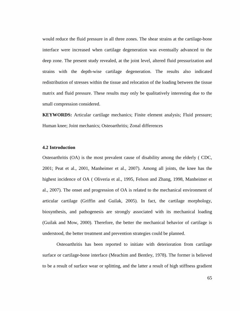
would reduce the fluid pressure in all three zones. The shear strains at the cartilage-bone

interface were increased when cartilage degeneration was eventually advanced to the

deep zone. The present study revealed, at the joint level, altered fluid pressurization and

strains with the depth-wise cartilage degeneration. The results also indicated

redistribution of stresses within the tissue and relocation of the loading between the tissue

matrix and fluid pressure. These results may only be qualitatively interesting due to the

small compression considered.

KEYWORDS: Articular cartilage mechanics; Finite element analysis; Fluid pressure;

Human knee; Joint mechanics; Osteoarthritis; Zonal differences

4.2 Introduction

Osteoarthritis (OA) is the most prevalent cause of disability among the elderly ( CDC,

2001; Peat et al., 2001, Manheimer et al., 2007). Among all joints, the knee has the

highest incidence of OA ( Oliveria et al., 1995, Felson and Zhang, 1998, Manheimer et

al., 2007). The onset and progression of OA is related to the mechanical environment of

articular cartilage (Griffin and Guilak, 2005). In fact, the cartilage morphology,

biosynthesis, and pathogenesis are strongly associated with its mechanical loading

(Guilak and Mow, 2000). Therefore, the better the mechanical behavior of cartilage is

understood, the better treatment and prevention strategies could be planned.

Osteoarthritis has been reported to initiate with deterioration from cartilage

surface or cartilage-bone interface (Meachim and Bentley, 1978). The former is believed

to be a result of surface wear or splitting, and the latter a result of high stiffness gradient

65

at cartilage-bone interface (Meachim and Bentley, 1978; Carter et al., 2004). An altered

mechanical environment, such as by stress, strain, and fluid flow, affects the biosynthesis

of chondrocytes (Wong and Carter, 2003), and eventually leads to tissue degeneration

and loss, and exposure of bone surface to direct joint contact.

When OA is initiated from the surface, it progresses layer by layer, from the

superficial zone, to the middle and eventually deep zones (Arokoski et al., 2000). During

this process, each layer of the tissue suffers from an altered mechanical environment, e.g.

the stress, strain, and fluid pressure in the deeper layer can be altered by degenerated

superficial layers.

The mechanics of depth-wise (layer by layer) progression of OA in the knee joint

must be affected by the multiple contacts between the cartilaginous tissues, including

femoral cartilage, meniscus, and tibial cartilage. A few factors may be important in the

contact mechanics of the knee. First, the 3D geometry of these tissues is obviously a

dominant parameter that determines the contact area and distribution of contact loading.

Second, the fluid pressurization in these tissues plays an essential role in the mechanical

functions of the knee, because the knee compression is associated with high fluid

pressure in these cartilaginous tissues (Ateshian and Hung, 2005). Additionally, the

depth-dependent tissue properties, often being characterized by three discrete zones, may

also affect the mechanical behavior of the joint.

Great progress has been made in computational OA modeling, with major

simplifications on the geometry including unrealistic boundary conditions, and on the

material properties including absence of fluid and fiber properties. For those studies with

66

fluid pressure considered, some assumed a spherical contact in the knee with no meniscus

(Wu et al., 2000, Federico et al., 2004, 2005); others modeled unconfined compression

testing only. The effect of PG depletion and collagen degradation was investigated by

reducing the modulus of the two constituents, respectively (Korhonen et al., 2003).

Unconfined geometry was used with a fibril reinforced model (Li et al., 1999). In another

study, OA was modeled in a depth-dependent manner (Saarakkala et al., 2010). The

depth-dependent properties were used for cartilage based on values reported in the

literature (Wilson et al., 2006). Again, unconfined compression geometry was used in the

study. A major progress was made recently in knee OA modeling when both 3D

geometry and fluid pressure in articular cartilage were implemented (Mononen et al.,

2012). In this latest study the fluid flow in the menisci was ignored, which could possibly

affect the prediction of the contact mechanics of the joint. Furthermore, the depth-

dependent mechanical properties were not incorporated in the study.

Computer modeling may provide an effective tool to examine the effect of

cartilage degeneration on contact mechanics and especially fluid pressure within the

intact joint. We attempted to study the contact mechanics with an anatomically accurate

finite element (FE) model of the normal and osteoarthritic knee joint. The material model

for the cartilaginous tissues included nonfibrillar matrix, fibers, fluid and depth-

dependent properties. We hypothesized that, due to perturbations induced by OA, the

fluid pressure in the tissue would be reduced with a given knee compression

(displacement-control). To examine this hypothesis a normal model was compared with

case studies whereby depth-wise progression of cartilage degeneration was implemented.

67

As a first step for our OA modeling of the knee, cartilage degeneration was assumed in

the high load-bearing region of the medial condyle. This is one of the regions where the

lesions are more likely progressed to deep layers (Seedholm et al., 1979, Andriacchi et

al., 2004, Carter et al., 2004), although OA lesions were also found in other sites of

femoral cartilage (Seedholm et al., 1979, Bae et al., 2010). The medial condyle was

chosen because it was believed to carry higher load compared to the lateral condyle

(Brown and Shaw, 1984). The medial condyle was reported to be more susceptible to OA

development in both normal (Temple et al., 2007) and ligament-deficient knees ( Maffulli

et al., 2003, Strobel et al., 2003, Tandogan et al., 2004). The medial condyle experienced

the most rapid lesion progression (Biswal et al., 2002).

4.3 Methods

The geometry of the model was reconstructed from MRI images of the right knee of a 27­

year-old male subject, who had no symptoms of OA (SPGR sequence, 625×625µm

resolution, Sagittal scan). The model included the distal femur, femoral cartilage,

meniscus, tibial cartilage, and proximal tibia (Fig. 4.1). The maximum thickness of the

femoral cartilage was approximately 2.8mm, and the maximum thickness of the menisci

was 8.4mm (Gu and Li, 2011).

68

Fig. 4.1. Finite element model of the tibiofemoral joint, showing the distal femur, proximal tibia, menisci, femoral and tibial cartilages. The tibial cartilage on the medial side is essentially covered by the medial meniscus (right knee, medial side shown on the left of the figure). The femoral cartilage is further shown with 8 layers of elements.

The cartilaginous tissues, i.e. femoral cartilage, menisci, and tibial cartilage, were

assumed as fibril-reinforced fluid-saturated materials. A fibril-reinforced constitutive law

was used which models the solid of the tissue as a linear nonfibrillar matrix that is

reinforced by a nonlinear fibrillar matrix (Li et al., 1999). Hence, two material properties

were required to define the nonfibrillar matrix, i.e. the elastic modulus Em and Poisson’s

ratio νm. The fibrillar matrix was characterized by elastic moduli in three orthogonal

directions. For the case of small deformations considered in the present study, these

69

moduli were simplified as linear functions of the corresponding tensile strain, e.g. for the

local x-direction

0 εε (4-1)Ex + Ex x , if ε x ≥ 0Ex =

0 , if ε x < 0

The compressive stiffness of the fibrillar matrix was neglected because the fibers

mainly support tensile loading. Note that the x-direction could be oriented in different

directions for different sites. Therefore, a 3D collagen orientation could be thus

incorporated. In order to describe the interstitial fluid flow, an orthotropic hydraulic

permeability was introduced per Darcy’s law, e.g. for the local x-direction

= −k p x (4-2)vx x f ,

where kx is the x-component of the permeability, which is the negative ratio of the x-

component of the fluid velocity, vx, and the x-component of the fluid pressure gradient,

pf ,x . Simply replacing the subscript x in Eqs. (4-1) and (4-2) with y or z would obtain the

relevant equations for the y or z direction.

The depth-dependent properties were incorporated for the femoral cartilage, i.e.

the tissue properties varied with the superficial, middle and deep zones, in the way

approximated previously (Li et al., 2000). In the superficial zone, the fibers were oriented

according to the split lines recorded from the surface (Below et al., 2002, adopted from

Fig. 2 in Gu and Li, 2011). In the middle zone, the fibers did not have any specific

orientation. In the deep zone, they were vertical to the cartilage-bone interface. In the

meniscus, the primary fibers were oriented in the circumferential direction. No preferred

fiber directions were considered for the tibial cartilage due to lack of data. 70

The surface-to-surface contact was defined between articulating surfaces using ABAQUS

6.10. Namely, contact was defined between: femoral cartilage and meniscus, femoral

cartilage and tibial cartilage, meniscus and tibial cartilage. No fluid flow was assumed

between cartilage and bone. The cartilages and bones were meshed independently.

However, in reality, the cartilage is firmly attached to the bone. There is no relative

motion at the cartilage-bone interface. This interface condition was modeled using the

TIE contact option provided by ABAQUS, i.e., femoral cartilage was tied to femur,

medial and lateral tibial cartilages were tied to tibia, and meniscus horns were tied to the

tibial cartilage at both ends of each meniscus.

A ramp compression of 0.1mm was applied in 1s on top of the femur while the

bottom of the tibia was fixed. The knee was in full extension. As a boundary condition,

the free articulating surface (which was not in contact) was assigned to zero fluid

pressure.

The consolidation procedure in ABAQUS was used to analyze the quasi-static

problem. For cartilaginous tissues, porous elements with fluid pressure were used. The

20-node quadratic elements were used for the femoral cartilage, and the 8-node linear

elements were used for tibial cartilage and meniscus. The choice of using different

element types for the cartilages was a result of compromise between faster contact

convergence and better fluid pressure distribution. The 20-node elements provide better

numerical accuracy for the fluid pressure but significantly slow down the contact

convergence. We used the 20-node elements for the femoral cartilage, because that was

the focus for results. The bones were meshed with solid elements. The fluid pressure in

71

the bones was not considered, because it is less significant in load support as compared to

that in cartilaginous tissues due to a 3-order higher stiffness of the bones.

In order to understand the mechanics of the depth-wise progression of OA, the

normal and three degenerative case studies were implemented computationally. In Case

1, the perturbations were implemented only in the superficial zone. In Case 2, the

perturbations were implemented in superficial and middle zones, and in Case 3, the

perturbations were implemented in all three zones. As discussed earlier, local cartilage

degeneration was implemented within the high load-bearing region of the medial condyle

of the femoral cartilage (Fig. 4.2, bounded by the dash line). All other tissues were

assumed normal. These three cases simulated the onset of cartilage degeneration from the

superficial zone and progression to the deep zone.

The following perturbations were implemented for the degenerated cartilage: the

permeability was increased by 50%, the Young’s modulus of fibrillar matrix was

decreased by 70%, the Young’s modulus of nonfibrillar matrix was decreased by 65%,

and the orientation of fibers was not set in any particular direction. The material

properties of normal tissues are summarized in Table (4-1), which were mainly based on

previous fibril-reinforced modeling with tissue explants (Li et al., 2000, Li et al., 2009).

We assumed no changes in the thickness of the degenerated cartilage, because only early

degeneration was considered. Therefore, the same tissue geometry was used for the

normal and three case studies.

72

Table (4-1). Material properties for the normal tissues (Modulus: MPa; Permeability: 10−3mm4/Ns). The x is the primary fiber direction, i.e. the split-line direction for the superficial zone, the depth direction for the deep zone for articular cartilage, and the circumferential direction for the meniscus. The y and z are normal to the primary fiber direction. The properties are the same in the y and z directions.

Tissue

Fibrillar matrix, Eq (4-1) Nonfibrillar matrix

Permeability, Eq (4-2)

Ex Ey or Ez Em 𝜐𝜐Rm kx ky or kz

Femoral cartilage

Deep zone

3 + 1600𝜀𝜀𝑥𝑥 0.9 + 480𝜀𝜀𝑦𝑦/𝑧𝑧 0.80 0.36 1.0 0.5

Middle

zone

2 + 1000𝜀𝜀𝑥𝑥 2 + 1000𝜀𝜀𝑦𝑦/𝑧𝑧 0.60 0.30 3.0 1.0

Superficial zone

4 + 2200𝜀𝜀𝑥𝑥 1.2 + 660𝜀𝜀𝑦𝑦/𝑧𝑧 0.20 0.16 1.0 0.5

Tibial cartilage 2 + 1000𝜀𝜀𝑥𝑥 2 + 1000𝜀𝜀𝑦𝑦/𝑧𝑧 0.26 0.36 2.0 1.0

Menisci 28 5 0.50 0.36 2.0 1.0

Bones E = 5000 𝜐𝜐 = 0.30

4.4 Results

All results presented here are for the end of ramp compression prior to relaxation. The

fluid pressure in the femoral cartilage is shown in Fig. 4.2 for a superficial layer and Fig.

4.3 for a deep layer. In either layer, no significant alteration in the pressure was seen in

the lateral condyle (left in figure) when cartilage degeneration advanced in the medial

condyle from the superficial to middle and then deep zones (Normal → Case 1 → Case 2

→ Case 3). The pore pressure in the medial condyle was substantially reduced with the

73

progression of degeneration. This again was true for the fluid pressure in either

superficial or deep layer.

The depth variation of the fluid pressure in the degeneration site is shown in Figs.

4.4-4.6. The pressure decreased with the tissue depth in all cases. However, the pressure

gradient in the tissue thickness direction reduced progressively with cartilage

degeneration for a given knee compression, with larger reduction in the superficial zone

(Fig. 4.4). The depth variation was also site-specific; it can be more easily seen in the

high load-bearing region (Figs. 4.5 and 4.6).

74

Normal Case 1

Fluid Pressure (MPa)

Case 2 Case 3

Fig. 4.2. Fluid pressure (MPa) at the normalized depth of 1/16 (superficial layer) for the normal femoral cartilage and three cases of local cartilage degeneration. Case 1: degeneration in the superficial zone; Case 2: degeneration in both superficial and middle zones; and Case 3: degeneration in all three zones. The site of degeneration is indicated with the dash lines (inferior view of the right knee, i.e. the medial condyle on the right).

75

Normal Case 1

Fluid Pressure (MPa)

Case 2 Case 3

Fig. 4.3. Fluid pressure (MPa) at the normalized depth of 13/16 (deep layer) for the normal femoral cartilage and three cases of local cartilage degeneration as defined in Fig. 4.2.

76

Depth

Flui

d Pr

essu

re (M

Pa)

Fig. 4.4. Variation of fluid pressure along the depth of the femoral cartilage, shown for a location in the central contact region of the medial condyle where cartilage degeneration occurred. The depth was normalized by the tissue thickness (0 = articulating surface; 1 = cartilage-bone interface). The pressure was calculated at the centroid of each element.

77

Normal Case 1

Fluid Pressure (MPa)

Case 3 Case 2

Fig. 4.5. Fluid pressure (MPa) in a sagittal plane of the medial condyle (cut position shown in Fig. 4.2) for the normal femoral cartilage and three cases of local cartilage degeneration as defined in Fig. 4.2. The articulating surface is at bottom and the anterior side is on the right.

78

Normal Case 1

Fluid Pressure (MPa)

Case 3 Case 2

Fig. 4.6. Fluid pressure (MPa) in a coronal plane of the medial condyle (cut position shown in Fig. 4.3) for the normal femoral cartilage and three cases of local cartilage degeneration as defined in Fig. 4.2. The articulating surface is at bottom and the lateral side is on the left.

The distribution of normal strain along the tissue depth was also altered with

degeneration in the medial condyle (Fig. 4.7). This strain was associated with the lateral

expansion of the tissue when compressed in the thickness direction. The strain was

smaller in the superficial zone because more tangentially oriented fibers there restrained

the lateral expansion. However, the first principal strain was actually higher in the

superficial zone than in the middle and most deep zones due to high shear strains at the

surface (not shown). The first principal strain in the deepest layer was the largest in Case

79

3 (Fig. 4.8), mostly because of large shear strains at the cartilage-bone interface in Case 3

(the lateral strain shown in Fig. 4.7 was not the largest at the deepest layer).

Depth

Late

ral S

train

Fig. 4.7. Lateral strain along the depth of the femoral cartilage, shown for a location in the central contact region of the medial condyle where cartilage degeneration occurred. This normal strain was in the direction parallel to the articulating surface and perpendicular to the split-line. The depth was normalized by the tissue thickness (0 = articulating surface; 1 = cartilage-bone interface). The normal strain was calculated at the centroid of each element.

As compared to the normal case, the shear strains at the cartilage-bone interface

were reduced by cartilage degeneration in the superficial zone (Fig. 4.9, Case 1 vs

Normal), and further reduced when degeneration progressed into the middle zone (Fig.

4.9, Case 2 vs Case 1). However, the shear strains were eventually raised above normal

when cartilage degeneration progressed into the deep zone (Fig. 4.9, Case 3 vs Normal).

80

Note that these shear strains were associated with shear stresses τzx and τz y , which might

cause shear failure at the cartilage-bone interface (z is the tissue thickness direction).

Normal Case 1

Principal Strain

Case 2 Case 3

Fig. 4.8. First principal strain at the normalized depth of 15/16 (deep layer) for the normal femoral cartilage and three cases of local cartilage degeneration as defined in Fig. 4.2. This is an inferior view of the right knee, i.e. the medial condyle is on the right.

81

Strain 𝛾𝛾𝑧𝑧𝑥𝑥 Strain 𝛾𝛾𝑧𝑧𝑦𝑦

Normal

Case 1

Case 2

Case 3

Fig. 4.9. Shear strains at the normalized depth of 15/16 (deep layer) for the normal femoral cartilage and three cases of local cartilage degeneration as defined in Fig. 4.2. This is shown for part of the medial condyle. The local xy-plane is parallel to the cartilage-bone interface. The corresponding shear stresses for the strains are τzx and τzy , which are parallel to the interface.

4.5 Discussion

The fluid pressurization in all cartilaginous tissues was considered in the proposed model

of cartilage degeneration in the human knee with anatomically accurate geometry of the

82

joint. The zonal differences were considered in order to simulate the progression of

degeneration from the superficial to deep zones. Our hypothesis was positively tested: for

a given compression (displacement-control), the model predicted reduced fluid

pressurization (Figs. 4.2-4.6) although water content increased with cartilage

degeneration. The fluid pressure can support a large portion of the load applied to

cartilage (Ateshian and Hung, 2005), which is believed to be part of the mechanism to

reduce the joint friction (McCutchen, 1962), and thus to reduce the chances of OA

initiation from the tissue surface. Furthermore, the reduction in the fluid pressure

observed in the present study for the case of displacement-control indicated increased

joint friction and increased load support by the tissue matrix in the case of joint-force­

control. Both may cause further progression of OA and deterioration of the tissue.

The onset of cartilage degeneration in an upper zone also resulted in reduced fluid

pressure in the lower zone, e.g. a degenerated superficial zone would reduce the fluid

pressure in both middle and deep zones (Fig. 4.4, Case 1). Since fluid pressurization

bears high loading for the tissue, this result agrees with the protective role of the surface

layer for the deep layer, as suggested by both experimental and computational studies

(Setton et al., 1993, Shirazi et al., 2008).

Furthermore, the fluid pressure reduced quickly when the degeneration started

from the superficial zone and progressed to the middle zone, then reduced at a lower rate

when the degeneration advanced to the deep zone (Fig. 4.4). This was most likely a

consequence of different fiber orientations in the three zones. In the superficial zone, the

fibers are oriented tangentially to resist lateral expansion under knee compression, and

83

thus great fluid pressure is produced. Some tangential fibers in the middle zone should

also contribute to increased fluid pressure. In the deep zone, however, the vertical fibers

are in compression, and thus do not significantly contribute to fluid pressurization.

Therefore, collagen degeneration in the deep zone would cause less fluid pressure change

in the tissue than degeneration in the superficial and middle zones.

The shear strains at the cartilage-bone interface were increased substantially with

cartilage degeneration to the deep zone (Fig. 4.9, Case 3 vs Normal). This was probably

because cartilage degeneration in the deep zone further increased the high gradient of the

material properties from deep cartilage to underlying bone. Great shear strains at the

cartilage-bone interface could cause microfractures, which eventually leads to OA (Radin

and Rose, 1986, Vener et al., 1992, Burr and Radin, 2003). The high gradients of material

properties are believed to increase the possibility of damage to the cartilage-bone

interface (Meachim and Bentley, 1978, Radin and Rose, 1986). Surprisingly, the shear

strains at the interface were reduced in Cases 1 and 2 prior to the progression of

degeneration into the deep zone (Fig. 4.9, Case 1 or 2 vs Normal). The reason was

probably due to the reduction of fluid pressure and its gradient in the tissue depth

direction while the material properties in the deep zone remained unchanged in Cases 1

and 2. Note that knee compression was given in the present study (displacement control).

The shear strains might not have been reduced in Cases 1 and 2, if the joint force had

been given (force-control).

Lower Young’s moduli and higher permeability were used in the present study to

simulate cartilage degeneration, in agreement with data from the literature (Armstrong

84

and Mow, 1982, Knecht et al., 2006). The compressive modulus of cartilage was reduced,

respectively, by 18% and 87.5%, and the water content was increased, respectively, by

79.9-81.6% and 84.1%, in moderate and advanced OA (Nieminen et al., 2004, Knecht et

al., 2006). According to another study, as a result of OA, the compressive and tensile

moduli of human articular cartilage were decreased by 55-68% and 72-83% respectively,

and the permeability was increased by 60-80% (Boschetti and Peretti, 2008). For the

human tibial cartilage, the compressive stiffness was decreased by 29% (Ding et al.,

1998); the compressive compliance was increased by 71% as a result of OA (Obeid et al.,

1994). Six months after anterior cruciate ligament transection, the compressive modulus

of canine cartilage was decreased by 25%, while the permeability was increased by ~48%

twelve weeks after the surgery (Setton et al., 1994, Setton et al., 1999). We have used

moderate values from these measurements.

Reduced surface fluid pressure with OA was also reported in the only similar

existing study (Mononen et al., 2012). It was found in that study that the stress

distribution through cartilage depth was also influenced by the orientation of superficial

fibers. The additional features of the present study included the fluid pressure in all

cartilaginous tissues and full consideration of the depth-dependent mechanical properties.

We further simulated the depth-wise cartilage degeneration from the superficial to deep

zones. As a consequence, the present results suggest that not only the degeneration in the

superficial layer reduced the fluid pressure in the deeper layers, which agrees with the

existing study (Mononen et al., 2012), but also that degeneration in the deeper layers

lowered the fluid pressure in the superficial layer.

85

A major limitation of the present study was due to the small knee compression

(100 µm) that was applied at a rather low rate (100 µm/s) in the computer simulation.

Our choice was a consequence of slow contact convergence and high demand in

computational time resulting from a high resolution of element mesh associated with the

zonal differences. Eight layers of elements were meshed in the tissue thickness direction

so there were 2, 4 and 2 layers of elements, respectively, for the superficial, middle and

deep zones. This mesh required several times more computational time, as compared to

the previous 4-layer mesh when the zonal differences were ignored (Gu and Li, 2011,

Kazemi et al., 2011). It took about a week to complete 1s simulation on a 4-CPU

workstation. In addition, we sometimes failed to obtain convergent results when larger or

faster compressions were applied. Further verifications are in progress. Because of the

small compression considered, one primary concern is whether the results were

compromised by the geometrical errors introduced during MRI segmentation and element

meshing, such as errors in surface curvature and tissue thickness. While such errors

indeed existed, they were probably at a lower level as compared to 100 µm. (The quality

of surface construction can be positively seen from the continuous variation in pore

pressure. The errors in geometry construction have been examined by independent

research groups, e.g. Li et al., 2001.) Other limitations included the omission of osmotic

pressure and the use of lab loading conditions.

The same compression was used in the present study, i.e. a displacement-control

was used for comparison. While the force-control loading protocol is often considered

more realistic, a knee joint with different stages of OA may not experience the same

86

force. As the OA develops, the patient tends to apply lower load on the diseased side

(Kaufman et al., 2001). On the other hand, it is more convenient and easier to interpret

the results when using a displacement-control in both computer simulations and lab tests.

Theoretically, the results from displacement control can be qualitatively interpreted to

that of force-control. Therefore, we chose the displacement control for simplicity.

The results presented here should be qualitatively correct, although the

magnitudes are not realistic because of the use of small and slow compression in the

present study. The alterations due to degeneration would be amplified in the case of a

physiologically realistic compression. This is because of the nonlinear and compression-

rate dependent load response of the joint. If a larger compression were applied, the fluid

pressure in the healthy cartilage would nonlinearly increase due to the normal collagen

network in the tissue, while the pressure in the degenerated cartilage would increase more

slowly due to a weak collagen network. For the same reason, if the same compression

were applied faster, the fluid pressure would increase faster in the healthy cartilage than

in the degenerated cartilage. In other words, the difference in the fluid pressurization in

the healthy and degenerated cartilages would be enlarged with the compression-

magnitude and compression-rate. This is understood from previous studies on cartilage

explants: both nonlinearity and strain-rate dependence of the load response of cartilage

are predominantly determined by the properties of collagen network (Li et al., 1999,

2003a, b).

The results of this investigation shed light on the effect of perturbation of material

properties and fibers orientation on knee joint mechanics, in the course of progression of

87

OA from cartilage surface to the cartilage-bone interface. Clinical studies suggest the

depth of cartilage defect as a parameter that characterizes OA severity (Brittberg and

Winalski, 2003). Computational modeling can be used to study the effect of this

parameter on the mechanics of knee joint. Furthermore, the role of defect depth in knee

joint mechanics can be better understood if computational models consider depth-

dependent properties embedded in an anatomical accurate geometry, as this study

showed. The findings of this study could be implemented in characterizing OA severity

based on the depth of cartilage injury. In fact, the development of OA is a multifactorial

phenomenon including alteration of tissue mechanical properties, perturbation of fiber

orientation, cartilage tissue loss, and the size and location of cartilage lesion (Brittberg

and Winalski, 2003, Guettler et al., 2004, Peña et al., 2007, Mononen et al., 2012). In this

study, the effect of the first two parameters was investigated, whereas the importance of

other factors will be investigated in future.

In summary, we have determined the alterations of fluid pressure and strains in

articular cartilage for the local tissue degeneration in the medial condyle of the femur.

These results may provide new information in understanding the progression of

osteoarthritis. As discussed earlier, cartilage degeneration resulted in reduced capability

of fluid pressurization and reduced pressure gradients in the tissue, which suggest

reduced lubrication in the joint and increased load support for the tissue matrix. Results

also suggest that once cartilage degeneration is initiated from the articulating surface, it

will eventually advance to the deep layer. This facilitation is achieved through the

reduction of fluid pressurization in all three zones with greater reduction in the superficial

88

zone, and damage to the depth-dependent structure of the tissue. In particular, cartilage

degeneration in the superficial zone may increase the possibility of damage to cartilage-

bone interface.

ACKNOWLEDGEMENTS

The present study was partially supported by the Natural Sciences and Engineering

Research Council of Canada, and the Canadian Institutes of Health Research.

CONFLICT OF INTEREST

The authors have no conflict of interest to disclose.

4.6 References

Andriacchi TP, Mündermann A, Smith RL, Alexander EJ, Dyrby CO, Koo S. A

framework for the in vivo pathomechanics of osteoarthritis at the knee. Ann Biomed Eng

2004;32:447-57.

Armstrong CG, Mow VC. Variations in the intrinsic mechanical properties of human

articular cartilage with age, degeneration, and water content. J Bone Joint Surg Am

1982;64:88-94.

Arokoski JP, Jurvelin JS, Väätäinen U, Helminen HJ. Normal and pathological

adaptations of articular cartilage to joint loading. Scand J Med Sci Sports 2000;10:186­

98.

Ateshian GA, Hung CT. Patellofemoral joint biomechanics and tissue engineering. Clin

Orthop Relat Res 2005;81:81-90.

89

Bae WC, Payanal MM, Chen AC, Hsieh-Bonassera ND, Ballard BL, Lotz MK, Coutts

RD, Bugbee WD, Sah RL. Topographic Patterns of Cartilage Lesions in Knee

Osteoarthritis. Cartilage 2010;1:10-19.

Below S, Arnoczky SP, Dodds J, Kooima C, Walter N. The split-line pattern of the distal

femur: A consideration in the orientation of autologous cartilage grafts. Arthroscopy

2002;18:613-7.

Biswal S, Hastie T, Andriacchi TP, Bergman GA, Dillingham MF, Lang P. Risk factors

for progressive cartilage loss in the knee: a longitudinal magnetic resonance imaging

study in forty-three patients. Arthritis Rheum 2002;46:2884-92.

Boschetti F, Peretti GM. Tensile and compressive properties of healthy and osteoarthritic

human articular cartilage. Biorheology 2008;45:337-44.

Brittberg M, Winalski CS. Evaluation of cartilage injuries and repair. J Bone Joint Surg

Am 2003;85-A Suppl 2:58-69.

Brown TD , Shaw DT. In vitro contact stress distribution on the femoral condyles. J

Orthop Res 1984;2:190-9.

Burr DB, Radin EL. Microfractures and microcracks in subchondral bone: are they

relevant to osteoarthrosis? Rheum Dis Clin North Am 2003;29:675-85.

Carter DR, Beaupré GS, Wong M, Smith RL, Andriacchi TP, Schurman DJ. The

mechanobiology of articular cartilage development and degeneration. Clin Orthop Relat

Res 2004;427:S69-77.

90

Centers for Disease Control and Prevention. Prevalence of self-reported arthritis or

chronic joint symptoms among adults--United States, MMWR Morb Mortal Wkly Rep

2002;51:948-50.

Ding M, Dalstra M, Linde F, Hvid I. Changes in the stiffness of the human tibial

cartilage-bone complex in early-stage osteoarthrosis. Acta Orthop Scand 1998;69:358-62.

Federico S, Herzog W, and Wu JZ. Erratum: effect of fluid boundary conditions on joint

contact mechanics and applications to the modelling of osteoarthritic joints, J Biomech

Eng 2005;127: 208–209.

Federico S, La Rosa G, Herzog W, and Wu JZ. Effect of fluid boundary conditions on

joint contact mechanics and applications to the modelling of osteoarthritic joints, J

Biomech Eng 2004;126:220–225.

Felson DT, Zhang Y. An update on the epidemiology of knee and hip osteoarthritis with

a view to prevention. Arthritis Rheum 1998;41:1343-55.

Griffin TM, Guilak F. The role of mechanical loading in the onset and progression of

osteoarthritis. Exerc Sport Sci Rev 2005;33:195-200.

Gu KB, Li LP. A human knee joint model considering fluid pressure and fiber orientation

in cartilages and menisci. Med Eng Phys 2011;33:497-503.

Guettler JH, Demetropoulos CK, Yang KH, Jurist KA. Osteochondral defects in the

human knee: influence of defect size on cartilage rim stress and load redistribution to

surrounding cartilage. Am J Sports Med 2004;32:1451-8.

91

Guilak F, Mow VC. The mechanical environment of the chondrocyte: a biphasic finite

element model of cell-matrix interactions in articular cartilage. J Biomech 2000;33:1663­

73.

Kaufman KR, Hughes C, Morrey BF, Morrey M, AN KN. Gait characteristics of patients

with knee osteoarthritis. J Biomech 2001;34:907-15.

Kazemi M, Li LP, Savard P, Buschmann MD. Creep behavior of the intact and

meniscectomy knee joints. J Mech Behav Biomed Mater 2011;4:1351-8.

Knecht S, Vanwanseele B, Stüssi E. A review on the mechanical quality of articular

cartilage - implications for the diagnosis of osteoarthritis. Clin Biomech (Bristol, Avon)

2006;21: 999-1012.

Korhonen RK, Laasanen MS, Töyräs J, Lappalainen R, Helminen HJ, Jurvelin JS. Fibril

reinforced poroelastic model predicts specifically mechanical behavior of normal,

proteoglycan depleted and collagen degraded articular cartilage. J Biomech

2003;36:1373-9.

Krishnan R, Park S, Eckstein F, Ateshian GA. Inhomogeneous cartilage properties

enhance superficial interstitial fluid support and frictional properties, but do not provide a

homogeneous state of stress. J Biomech Eng 2003;125:569-77.

Li LP, Buschmann MD, Shirazi-Adl A. A fibril reinforced nonhomogeneous poroelastic

model for articular cartilage: inhomogeneous response in unconfined compression. J

Biomech 2000;33:1533-1541.

Li LP, Buschmann MD, Shirazi-Adl A. Strain-rate dependent stiffness of articular

cartilage in unconfined compression. J Biomech Eng 2003;125,161-168.

92

Li LP, Buschmann MD and Shirazi-Adl A. Erratum: Strain-rate dependent stiffness of

articular cartilage in unconfined compression. J Biomech Eng 2003;125,566.

Li LP, Cheung JTM, Herzog W. Three-Dimensional Fibril-Reinforced Finite Element

Model of Articular Cartilage. Med Biol Eng Comput 2009;47:607-615.

Li G, Lopez O, Rubash H. Variability of a three-dimensional finite element model

constructed using magnetic resonance images of a knee for joint contact stress analysis. J

Biomech Eng 2001;123:341-346.

Li LP, Soulhat J, Buschmann MD, Shirazi-Adl A. Nonlinear analysis of cartilage in

unconfined ramp compression using a fibril reinforced poroelastic model. Clin Biomech

(Bristol, Avon) 1999;14:673-82.

Maffulli N, Binfield PM, King JB. Articular cartilage lesions in the symptomatic anterior

cruciate ligament-deficient knee. Arthroscopy 2003;19:685-90.

Manheimer E, Linde K, Lao L, Bouter LM, Berman BM. Meta-analysis: acupuncture for

osteoarthritis of the knee. Ann Intern Med 2007;146:868-77.

Mccutchen CW. The frictional properties of animal joints. Wear 1962;5:1-17.

Meachim G, Bentley G. Horizontal splitting in patellar articular cartilage. Arthritis

Rheum 1978;21:669-74.

Mononen ME, Mikkola MT, Julkunen P, Ojala R, Nieminen MT, Jurvelin JS, Korhonen

RK. Effect of superficial collagen patterns and fibrillation of femoral articular cartilage

on knee joint mechanics-a 3D finite element analysis. J Biomech 2012;45:579-87.

93

Nieminen HJ, Saarakkala S, Laasanen MS, Hirvonen J, Jurvelin JS, Töyräs J. Ultrasound

attenuation in normal and spontaneously degenerated articular cartilage. Ultrasound Med

Biol 2004;30:493-500.

Obeid EM, Adams MA, Newman JH. Mechanical properties of articular cartilage in

knees with unicompartmental osteoarthritis. J Bone Joint Surg Br 1994;76:315-9.

Oliveria SA, Felson DT, Reed JI, Cirillo PA, Walker AM. Incidence of symptomatic

hand, hip, and knee osteoarthritis among patients in a health maintenance organization.

Arthritis Rheum 1995;38:1134-41.

Peat G, Mccarney R, Croft P. Knee pain and osteoarthritis in older adults: a review of

community burden and current use of primary health care. Ann Rheum Dis 2001;60:91-7.

Peña E, Calvo B, Martínez MA, Doblaré M. Effect of the size and location of

osteochondral defects in degenerative arthritis. A finite element simulation. Comput Biol

Med 2007;37:376-87.

Radin EL, Rose RM. Role of subchondral bone in the initiation and progression of

cartilage damage. Clin Orthop Relat Res 1986;213:34-40.

Saarakkala S, Julkunen P, Kiviranta P, Mäkitalo J, Jurvelin JS, Korhonen RK. Depth-

wise progression of osteoarthritis in human articular cartilage: investigation of

composition, structure and biomechanics. Osteoarthritis Cartilage 2010;18:73-81.

Seedholm BB, Takeda T, Tsubuku M, Wright V. Mechanical factors and patellofemoral

osteoarthrosis. Ann Rheum Dis 1979;38:307-16.

94

Setton LA, Elliott DM, Mow VC. Altered mechanics of cartilage with osteoarthritis:

human osteoarthritis and an experimental model of joint degeneration. Osteoarthritis

Cartilage 1999;7:2-14.

Setton LA, Mow VC, Müller FJ, Pita JC, Howell DS. Mechanical properties of canine

articular cartilage are significantly altered following transection of the anterior cruciate

ligament. J Orthop Res 1994;12:451-63.

Setton LA, Zhu W, Mow VC. The biphasic poroviscoelastic behavior of articular

cartilage: role of the surface zone in governing the compressive behavior. J Biomech

1993;26:581-92.

Shirazi R, Shirazi-Adl A. Computational biomechanics of articular cartilage of human

knee joint: effect of osteochondral defects. J Biomech 2009;42:2458-65.

Shirazi R, Shirazi-Adl A, Hurtig M. Role of cartilage collagen fibrils networks in knee

joint biomechanics under compression. J Biomech 2008;41:3340-8.

Strobel MJ, Weiler A, Schulz MS, Russe K, Eichhorn HJ. Arthroscopic evaluation of

articular cartilage lesions in posterior-cruciate-ligament-deficient knees. Arthroscopy

2003;19:262-8.

Tandogan RN, Taşer O, Kayaalp A, Taşkiran E, Pinar H, Alparslan B, Alturfan A.

Analysis of meniscal and chondral lesions accompanying anterior cruciate ligament tears:

relationship with age, time from injury, and level of sport. Knee Surg Sports Traumatol

Arthrosc 2004;12:262-70.

95

Temple MM, Bae WC, Chen MQ, Lotz M, Amiel D, Coutts RD, Sah RL. Age- and site-

associated biomechanical weakening of human articular cartilage of the femoral condyle.

Osteoarthritis Cartilage 2007;15:1042-52.

Vener MJ, Thompson RC, Lewis JL, Oegema TR. Subchondral damage after acute

transarticular loading: an in vitro model of joint injury. J Orthop Res 1992;10:759-65.

Wilson W, Van Burken C, Van Donkelaar C, BUMA P, Van Rietbergen B, Huiskes R.

Causes of mechanically induced collagen damage in articular cartilage. J Orthop Res

2006;24:220-8.

Wong M, Carter DR. Articular cartilage functional histomorphology and

mechanobiology: a research perspective. Bone 2003;33:1-13.

Wu JZ, Herzog W, Epstein M. Joint contact mechanics in the early stages of

osteoarthritis. Med Eng Phys 2000;22:1-12.

96

Chapter Five: Load Bearing Characteristics of the Knee Joint Deteriorates with the Defect Depth of Articular Cartilage

5.1 Abstract

Osteoarthritis is associated with alterations in cartilage mechanical properties and tissue

loss. The focal cartilage defect is a typical type of tissue loss. The present study

investigated the altered mechanics of human knee joint due to focal defects. The focus

was on the fluid pressurization and its load support in cartilage. Ten normal and defect

cases were analyzed using an anatomically accurate finite element model of the knee.

Fluid pressurization, anisotropic fibril-reinforcement, and depth-dependent mechanical

properties were modeled for articular cartilages and menisci. The focal defects were

considered in both condyles within high load-bearing regions. Both displacement and

force controls were simulated. A reduced load bearing capacity was seen in the vicinity

of the defect region, which was similar to the case of cartilage degeneration investigated

previously. A deeper defect caused more fluid pressure reduction in the surrounding

region. However, a partial defect did not necessarily cause a fluid pressure reduction in

the remaining underlying cartilage: the fluid pressure could increase in some scenarios,

which was different from the case of cartilage degeneration. Cartilage defects also

increased the shear strain at the cartilage-bone interface, which was more significant with

a full-thickness defect. The remaining defect tissue could still support substantial loading,

when it was in contact with the mating surface. The consequence of cartilage defect also

depended on the defect sites. Finally, the creep response could be interpreted from the

97

relaxation response with knowledge of the nonlinear and strain-rate dependent behavior

of articular cartilage.

KEYWORDS: Articular cartilage mechanics; Cartilage focal defect; Finite element

analysis; Fluid pressure; Knee joint mechanics

5.2 Introduction

Osteoarthritis (OA) is a leading cause of disability among the elderly, and it has been

reported as the most prevalent joint disease in the USA (Peat et al., 2001, Manheimer et

al., 2007). One scenario of OA is to start from the surface of articular cartilage, and attack

deeper layer until reach the bone (Andriacchi et al., 2004, Saarakkala et al., 2010). Once

deep layers of cartilage are destroyed, bone is exposed to the joint contact. The knee joint

has the highest prevalence of OA (Oliveria et al., 1995, Felson and Zhang, 1998,

Manheimer et al., 2007). The prevalence and cost of knee OA was high in the past and is

expected to remain high in at least the next two decades (Lethbridge-Cejku et al., 2004,

Manheimer et al., 2007). The development of OA is not yet fully understood. The

interplay between cartilage structure and mechanical loading, however, is believed to be a

pathway in the OA development.

Perturbation of the composition and structure of cartilage may be a necessary step

to initiate OA (McDevitt and Muir, 1976, Stockwell et al., 1983, Guilak et al., 1994).

Cartilage is mainly composed of a solid matrix and a fluid (Mow and Ratcliffe, 1997).

The solid matrix is composed of collagen fibers and nonfibrillar proteoglycan matrix that

98

mostly support the tensile and compressive loading, respectively. Cartilage is often

divided into three zones: superficial, middle, and deep zones (Mow et al., 1980, Mow and

Ratcliffe, 1997). Fibers are mostly parallel to the surface in the superficial zone,

randomly-oriented in the middle zone, and perpendicular to the cartilage-bone interface

in the deep zone.

Fluid pressurization plays an essential role in the mechanics of a joint, lubricating

the joint and preventing the matrix of cartilage from excessive loading (McCutchen,

1962, Walker et al., 1968, Ateshian and Hung, 2005). Fluid pressurization contributes to

load support of the joint at different scales during different loading phases (Mow et al.,

1984, Herberhold et al., 1999, Li et al., 2002). For example, load is applied on the knee

joint in a fraction of a second during gait which is associated with high fluid

pressurization, whereas standing for a long time might be associated with a lower fluid

pressure in the knee. Moreover, the alteration in fluid pressurization is one of the

symptoms in the early OA (Maroudas, 1976, Maroudas and Venn, 1977, Venn and

Maroudas, 1977, Maroudas et al., 1985). Recently, we demonstrated a weaker fluid

pressurization in a degenerated knee, using an anatomically accurate model of the knee

joint (Dabiri and Li, 2013).

Several parameters may play roles in the interplay between defect progression and

mechanical loading including defect depth, size, location, and properties of cartilage

associated with the defect (Seedholm et al., 1979, Noyes and Stabler, 1989, Brittberg and

Winalski, 2003). Experimental studies encounter difficulties when investigating the effect

of each of these parameters. The consequence of each parameter is difficult to

99

differentiate as they often evolve simultaneously. Numerical simulation can be recruited

to study the development of OA and the role of each parameter in the progression of OA,

as has been reported in the literature (Haut Donahue et al., 2003, Ramaniraka et al., 2005,

Peña et al., 2007). In a recent study, the contact mechanics of the knee joint was

investigated in the presence of cartilage degeneration with alterations in mechanical

properties including fiber orientation (Mononen et al., 2012). The study, however, did not

consider the fluid pressure in menisci and full depth-dependent properties of cartilages,

and only considered the short-term behavior of the knee joint. The significance of defect

size in the mechanics of the knee joint was reported using an elastic model (Peña et al.,

2007). The mechanics of cartilage defect has also been investigated with two-dimensional

explant geometries (Duda et al., 2005).

The defect depth is a criterion to categorize the severity of a cartilage defect

(Noyes and Stabler, 1989, Brittberg and Winalski, 2003). For example, the International

Cartilage Repair Society (ICRS) has a classification system for cartilage defect which is

based on the progression of defect from cartilage surface to cartilage-bone interface

(Brittberg and Winalski, 2003). Therefore, the objective of the present study was to

determine the alteration in fluid pressurization in the human knee joint in different stages

of defect progression from cartilage surface to cartilage-bone interface.

5.3 Methods

The geometry of the knee model was reconstructed from the MRI images of the right leg

of a male subject who was 27 years old with no leg injury (Gu and Li, 2011, Kazemi et

100

al., 2011, Kazemi et al., 2012). The model was composed of femur, femoral cartilage,

menisci, tibial cartilage, and tibia. The commercial finite element package ABAQUS

6.10 (Simulia, Providence, USA) was used for the finite element analysis with custom

defined material model. The femur and tibia were modeled as linearly elastic. Articular

cartilages and menisci were considered fluid-saturated materials reinforced by a nonlinear

fiber network, using a previously developed fibril-reinforced model of cartilage (Li et al.,

2002). The depth-varying tissue properties of the femoral cartilage were also incorporated

as per a recent study (Dabiri and Li, 2013)

The surface-to-surface contact modeling in ABAQUS was considered between

femoral cartilage and tibial cartilage, femoral cartilage and menisci, and tibial cartilage

and menisci. Using the TIE option in ABAQUS, the femoral cartilage was fixed to the

femur, and the tibial cartilage was fixed to the tibia. The horns of menisci were also tied

to the tibia.

Two loading conditions were considered: (1) Ramp compression of 500 µm

applied in 5s followed by relaxation up to 1000s; and (2) Ramp compressive force of

387.76 N applied in 5s followed by creep. This force was taken to be the same as

obtained at 500 µm compression. In either case, the compressive displacement or force

was applied on the top of femur with fixed bottom of tibia.

Cartilage defects can be developed in different sites (Seedholm et al., 1979, Bae et

al., 2010). We focused on the depth-wise advancement of defect in the medial femoral

cartilage as this region is more vulnerable to the development of lesions (Biswal et al.,

2002, Maffulli et al., 2003, Strobel et al., 2003, Tandogan et al., 2004, Temple et al.,

101

2007). Three types of cartilage defect were considered: (1) Superficial defect refers to the

defect in the superficial zone only (tissue loss in the zone); (2) Middle defect refers to the

defect in the superficial and middle zones; and (3) Deep defect refers to the defect in all

three zones (full-thickness loss). A superficial defect in the lateral femoral cartilage was

also examined for comparison.

In addition to the loading conditions, site and depth of defect, another factor

considered was the contact condition of the defect cartilage to its mating surface. Both

scenarios were implemented in the modeling: defect contact or no defect contact. Both

scenarios are possible, because patients tend to adjust their gait when OA develops

(Kaufman et al., 2001). Considering the combinations of all these factors, 10 cases were

investigated in this study (Table 5-1).

102

Table (5-1). Ten cases investigated in the present study. Three cartilage conditions were considered: normal cartilage, defects in the medial and lateral condyles, respectively; three defect depths were also assumed for the medial condyle defect: the defect in the superficial zone only, the defect up to the middle zone and the defect up to the deep zone. Both force and displacement controls (creep and relaxation) were simulated. In cases 6 and 7, no contact was assumed between the defected cartilage and its mating surface.

Loading & Normal Medial condyle defect Lateral condyle defect

contact cartilage

conditions Superficial Middle Deep Superficial

Displacement Case 1 Defect Case 2 Case 3 Case 4 Case 5

control contact

No Case 6 Case 7

defect

contact

Force control Case 8 Defect Case 9 Case 10

contact

5.4 Results

For the same knee compression, the short-term surface fluid pressure in the medial

condyle decreased with the defect depth (Fig. 5.1). The long-term fluid pressure

experienced less alteration with the defect, with some alteration in the pressure

distribution, surprisingly a little more significant with the middle defect (Fig. 5.2).

Furthermore, the fluid pressure in the lateral condyle was merely affected by the defect in

the medial condyle. A redistribution of the fluid pressure was more obvious when the

103

defect was progressed to full-thickness (Fig. 5.1). Note only the fluid pressures in the

unaffected cartilage are shown in Figs. 5.1 and 5.2.

(a) Case 1 (b) Case 2

Fluid Pressure (MPa)

(d) Case 4 (c) Case 3

Fig. 5.1. Surface fluid pressure in the femoral cartilage at 500µm compression prior to relaxation. (a) Normal model (Case 1), (b) Superficial defect model (Case 2), (c) Middle defect model (Case 3), and (d) Full-thickness defect model (Case 4). Defect contact was assumed in the three defect models (Cases 2-4). The medial condyle is on the right. This is an inferior view of the right knee.

104

(a) Case 1 (b) Case 2

Fluid Pressure (MPa)

(d) Case 4 (c) Case 3

Fig. 5.2. Surface fluid pressure in the femoral cartilage during late relaxation of 500µm compression (at 1000s). These are the same cases as shown in Fig. 5.1.

105

When the defect cartilage was in contact with its mating surface (Cases 2-4), a

decreased fluid pressure in the defect region was observed in the case of the superficial

defect as compared to the normal case (Fig. 5.3a vs 5.3b). However, a drastically raised

pressure in the defect region was seen in the case of middle defect (Fig. 5.3). On the other

hand, if the defect cartilage was not in contact with its mating surface (Cases 6 and 7), the

fluid pressure in the vicinity of defect decreased with defect depth (Fig. 5.4). The depth

variation of the pressure was also altered with the defect depth (Fig. 5.4)

106

(a) Case 1 (b) Case 2

(c) Case 3 (d) Case 4

Fluid Pressure (MPa)

Fig. 5.3. Fluid pressure in the layer of normalized depth of 1/16 at 500µm compression prior to relaxation. For the partial-thickness defect models, the fluid pressure in the defect region is shown for the new surface layer, i.e. at the depth of 5/16 (Case 2) and 13/16 (Case 3) respectively. Defect contact was assumed in the three defect models (Cases 2-4). The medial condyle is on the right.

107

Fluid Pressure (MPa)

(a) Case 1

(b) Case 6

(c) Case 7

Fig. 5.4. Fluid pressure in a sagittal plane of the femoral cartilage at 500µm compression prior to relaxation, shown for the high load bearing region of the medial condyle. (a) Normal model (Case 1), (b) Superficial defect model (Case 6), and (c) Middle defect model (Case 7). No defect contact was assumed in the defect models (Cases 6-7). The anterior side is on the left.

The reaction force of the defect joint could increase to above or decrease to below

the normal value depending on the contact condition at the defect region and the loading

phase (Fig. 5.5, displacement control). When the defect contact was considered (Cases 2­

4), the short-term reaction force was the highest in the case of middle defect, but the

long-term reaction force reduced with the defect depth (Fig. 5.5a). When the defect

108

contact was not considered (Cases 6-7), the reaction force was virtually the same for the

two defect cases, which was also close to the one for Case 4 (Fig. 5.5b).

The effect of a lateral defect on fluid pressure contours was more noticeable as

compared to a medial defect (Fig. 5.6). Specifically, two high-fluid pressure regions were

observed in the lateral defect while there was only one high-fluid pressure region in the

normal model.

The shear strain component in the cartilage-bone interface was altered by the

defect depth (Fig. 5.7). The superficial defect did not cause noticeable change in the shear

strain. However, the middle and deep defects produced obvious changes in the shear

strain. The location of peak shear strain moved toward defect rim as the defect advanced

to the deeper layer, and also the distribution of shear strain was altered.

For the cases of force control (Cases 8-10), the increase in the fluid pressure in the

defect region was more obvious than for the displacement control, especially for the

defect in the lateral condyle (Fig. 5.8).

109

(a)

(b) Fig. 5.5. Reaction force in the knee as a function of time for the ramp compression of 500µm followed by relaxation. (a) Defect contact was assumed in the defect models (Peak forces: Case 1: 387.764; Case 2: 363.614; Case 3: 396.252; Case 4: 288.13N); and (b) No defect contact was assumed in Cases 6 and 7 (Peak forces: Case 6: 309.457; Case 7: 293.578N).

110

Fluid Pressure (MPa)

(a) Case 1

(b) Case 2

(c) Case 5 Fig. 5.6. Surface fluid pressure in the femoral cartilage at 500µm compression prior to relaxation. (a) Normal model (Case 1), (b) Superficial defect in the medial condyle (Case 2), and (c) Superficial defect in the lateral condyle (Case 5). Defect contact was assumed in the defect models.

111

(a) Case 1 (b) Case 2

Shear strain

(c) Case 3 (d) Case 4

Fig. 5.7. Shear strain in the deepest cartilage layer during late relaxation of 500µm compression (at 1000s). (a) Normal model (Case 1), (b) Superficial defect model (Case 2), (c) Middle defect model (Case 3), and (d) Deep defect model (Case 4). Defect contact was assumed in the defect models (Cases 2-4). The medial condyle is on the right.

112

Fluid Pressure (MPa)

(a) Case 8

(b) Case 9

(c) Case 10

Fig. 5.8. Surface fluid pressure in the femoral cartilage at 387.76N compressive force prior to creep in the layer of normalized depth of 1/16. (a) Normal model (Case 8), (b) Superficial defect in the medial condyle (Case 9), and (c) Superficial defect in the lateral condyle (Case 10). For the defect models, the fluid pressure in the defect region is shown for the new surface layer, i.e. at the depth of 5/16. Defect contact was assumed in the two defect models (Cases 9-10). The medial condyle is on the right.

113

Forc

e (N

) 400

300 Loading Phase for creep (constant loading rate)

200

100 Loading Phase for relaxation (loading rate increases with time)

0 0 1 2 3 4 5

Time (s)

Fig. 5.9. Reaction force in the knee as a function of time during the loading phase for the cases of creep and stress relaxation. In the case of relaxation, the knee joint experienced a loading rate that started at a small value then increased with time, while in the case of creep, the loading rate was constant. The curve for the case of relaxation was taken from Fig. 5.5 for the normal joint.

5.5 Discussion

Generally speaking, the load bearing capacity associated with fluid pressurization was

weakened in the vicinity of the defect region (Figs. 5.1 and 5.2), but the remaining defect

cartilage may be more pressurized on the spot (Fig. 5.3c), if it was in contact with its

mating surface. In the case of displacement control, it meant lowered fluid pressure in the

vicinity of the defect region, which further decreased with the defect depth (Fig. 5.1). In

114

the case of force control, a weakened load bearing from fluid pressurization in the

vicinity of the defect meant increased fluid pressure in the remaining defect cartilage

(Fig. 5.8), in order to maintain the load support in the joint. In any case, a redistribution

of the fluid pressure has been observed in the defect region and its vicinity (Figs. 5.1-5.4,

5.6 and 5.8), as a result of load reallocation in the joint.

The reduced load bearing capability from fluid pressurization was not obviously

seen in the case of creep (Fig. 5.8), because the same force was maintained in the normal

and defect joints, as mentioned above. In other words, larger compressive displacement

or faster compression must be produced in the defect joint in order to produce the same

reaction force as that for the normal joint. In fact, a higher peak fluid pressure was seen in

creep than in relaxation for the normal joint (Fig. 5.8a vs 5.1a), although the same force

was applied in 5s in both creep and relaxation (Fig. 5.9). This phenomenon can be

explained by the nonlinear response of the knee (Li and Gu, 2011) and strain-rate

dependent response of articular cartilage (Li and Herzog, 2004). For the case of

relaxation, the compression rate (displacement/time) was constant, corresponding to a

lower loading rate (force/time) at the beginning and a higher loading rate at the end of the

loading phase (Fig. 5.9). For the case of creep, however, the loading rate was constant

during the loading phase, resulting in a higher compression rate at the beginning (but a

lower compression rate at the end) of the loading phase as compared to the case of

relaxation. The faster early compression in turn produced a higher fluid pressure during

early compression due to the strain-rate dependence of cartilage (Li and Herzog, 2004).

This higher fluid pressure did not have sufficient time to dissipate although the

115

compression was slowed down in the late loading phase. Therefore, we see a higher peak

fluid pressure in creep than in relaxation even the reaction forces were identical at the end

of the loading phase.

As indicated above, the creep behavior can be somehow understood from the

relaxation behavior, although they might look differently. On the other hand, modeling

stress relaxation is computationally less expensive than modeling creep, because a faster

increasing fluid pressure in creep results in a slower numerical convergence and also

because creep takes much longer time to complete (Li et al., 2008). Therefore, the present

study was focused on the stress relaxation (displacement-controlled) behavior of the knee

joint while creep response (force-controlled) was also modeled.

The contact condition at the defect region played a significant role in the load

support of the joint although the defect size was small (Figs. 5.4 and 5.5). The remaining

defect cartilage still supported substantial loading when it was in contact with its mating

surface (Fig. 5.5a, Cases 2 and 3 compared to Case 1). The reaction force in the knee was

significantly lower, if the remaining defect cartilage lost contact with its mating surface,

even the rest normal surfaces remained in contact (Fig. 5.5, Cases 6 and 7 vs Cases 2 and

3). This result indicated significant load changes in the defect joint from a slight gait

adjustment by a patient, as people often do when they suffer from OA (Kaufman et al.,

2001).

The effect of cartilage defect on the fluid pressurization was also dependent on

the defect site (Figs. 5.6 and 5.8). More results for the defect in the medial condyle are

presented in this paper, because this region is considered more vulnerable to the

116

development of lesions (Biswal et al., 2002, Maffulli et al., 2003, Strobel et al., 2003,

Tandogan et al., 2004, Temple et al., 2007).

The effect of cartilage defect on the fluid pressurization diminished with

relaxation and creep time (Figs. 5.1 vs 5.2), which was expected as fluid pressurization in

the tissue decays with stress relaxation and creep. However, one would still expect the

negative impact of the defect on the long-term stresses and strains of the tissue matrix, as

we see the shear strains in the region increased with the defect depth (Fig. 5.7). This

escalated shear strain may increase the chances of OA following microfracture at the

cartilage-bone interface (Radin and Rose, 1986, Vener et al., 1992, Burr and Radin,

2003). These results agree with previous studies on the importance of the tissue integrity

(Setton et al., 1993, Shirazi et al., 2008).

The effects of focal cartilage defect and degeneration on fluid pressurization were

similar in some ways and different in other ways. Both caused the reduced capacity of

fluid pressurization in the vicinity of the defect or degeneration; the reductions were

positively correlated to the depth of degeneration or defect (the effect of cartilage

degeneration was reported in Dabiri and Li, 2013). However, partial cartilage defects did

not necessarily cause fluid pressure reduction in the remaining underlying layers (Figs.

5.3 and 5.8) as it occurred in cartilage degeneration (Dabiri and Li, 2013). A defect

advanced to the middle zone resulted in a substantially higher fluid pressure in the deep

zone (Fig. 5.3c), but a degeneration advanced to the same zone caused lower fluid

pressure in the deep zone (Dabiri and Li, 2013), as compared to the normal case.

117

The major limitation of the present study was the use of non-physiological

loadings, which were relatively small (< 400 N) and slowly applied to the joint (5 s).

These loading protocols were used to avoid slow numerical convergence. While the fluid

pressures obtained were still low (0-4 MPa), they were close to measured contact

pressures in the knee joints. Therefore, the results presented here are still practically

interesting. Furthermore, the qualitative results would remain the same, if larger and

faster loadings were used.

In summary, focal cartilage defects substantially compromise the capability of the

fluid pressurization in articular cartilage and the load-bearing in the joint. Furthermore,

load bearing characteristics of the knee joint deteriorates with the defect depth of articular

cartilage. The altered mechanics of the knee are also influenced by the sites of defects

and the contact conditions in the defect regions.

Acknowledgments

Funding: the Natural Sciences and Engineering Research Council of Canada.

Conflict of Interests: the authors have no conflict of interest to declare.

Ethical approval: E-22593, University of Calgary, for the use of MRI of human subjects.

5.6 References

Andriacchi TP, Mündermann A, Smith RL, Alexander EJ, Dyrby CO, Koo S. A

framework for the in vivo pathomechanics of osteoarthritis at the knee. Ann Biomed Eng

2004;32:447-57.

118

Ateshian GA, Hung CT. Patellofemoral joint biomechanics and tissue engineering. Clin

Orthop Relat Res 2005;436:81-90.

Bae WC, Payanal MM, Chen AC, Hsieh-Bonassera ND, Ballard BL, Lotz MK, Coutts

RD, Bugbee WD, Sah RL. Topographic Patterns of Cartilage Lesions in Knee

Osteoarthritis. Cartilage 2010;1:10-19.

Biswal S, Hastie T, Andriacchi TP, Bergman GA, Dillingham MF, Lang P. Risk factors

for progressive cartilage loss in the knee: a longitudinal magnetic resonance imaging

study in forty-three patients. Arthritis Rheum 2002;46:2884-92.

Brittberg M, Winalski CS. Evaluation of cartilage injuries and repair. J Bone Joint Surg

Am 2003;85-A Suppl 2:58-69.

Burr DB, Radin EL. Microfractures and microcracks in subchondral bone: are they

relevant to osteoarthrosis? Rheum Dis Clin North Am 2003;29:675-85.

Dabiri Y, Li LP. Altered knee joint mechanics in simple compression associated with

early cartilage degeneration. Comput Math Methods Med 2013;2013:1-11,

http://dx.doi.org/10.1155/2013/862903.

Duda GN, Maldonado ZM, Klein P, Heller MO, Burns J, Bail H. On the influence of

mechanical conditions in osteochondral defect healing. J Biomech 2005;38:843-51.

Felson DT, Zhang Y. An update on the epidemiology of knee and hip osteoarthritis with

a view to prevention. Arthritis Rheum 1998;41:1343-55.

Gu KB, Li LP. A human knee joint model considering fluid pressure and fiber orientation

in cartilages and menisci. Med Eng Phys 2011;33:497-503.

119

Guilak F, Ratcliffe A, Lane N, Rosenwasser MP, Mow VC. Mechanical and biochemical

changes in the superficial zone of articular cartilage in canine experimental osteoarthritis.

J Orthop Res 1994;12:474-84.

Haut Donahue TL, Hull ML, Rashid MM, Jacobs CR. How the stiffness of meniscal

attachments and meniscal material properties affect tibio-femoral contact pressure

computed using a validated finite element model of the human knee joint. J Biomech

2003;36:19-34.

Herberhold C, Faber S, Stammberger T, Steinlechner M, Putz R, Englmeier KH, Reiser

M, Eckstein F. In situ measurement of articular cartilage deformation in intact

femoropatellar joints under static loading. J Biomech 1999;32:1287-95.

Kaufman KR, Hughes C, Morrey BF, Morrey M, An KN. Gait characteristics of patients

with knee osteoarthritis. J Biomech 2001;34:907-15.

Kazemi M, Li LP, Buschmann MD, Savard P. Partial meniscectomy changes fluid

pressurization in articular cartilage in human knees. J Biomech Eng 2012;134:021001.

Kazemi M, Li LP, Savard P, Buschmann MD. Creep behavior of the intact and

meniscectomy knee joints. J Mech Behav Biomed Mater 2011;4:1351-58.

Korhonen RK, Laasanen MS, Töyräs J, Lappalainen R, Helminen HJ, Jurvelin JS. Fibril

reinforced poroelastic model predicts specifically mechanical behavior of normal,

proteoglycan depleted and collagen degraded articular cartilage. J Biomech

2003;36:1373-79.

Lethbridge-Cejku M, Schiller JS, Bernadel L. Summary health statistics for U.S. adults:

National Health Interview Survey, 2002. Vital Health Stat 2004;10:1-151.

120

Li LP, Buschmann MD, Shirazi-Adl A. The role of fibril reinforcement in the mechanical

behavior of cartilage. Biorheology 2002;39:89-96.

Li LP, Gu KB. Reconsideration on the use of elastic models to predict the instantaneous

load response of the knee joint. Proc Inst Mech Eng H 2011;225:888-96.

Li LP, Herzog W. Strain-rate dependence of cartilage stiffness in unconfined

compression: the role of fibril reinforcement versus tissue volume change in fluid

pressurization. J Biomech 2004;37:375-82.

Li LP, Korhonen RK, Iivarinen J, Jurvelin JS, Herzog W. Fluid pressure driven fibril

reinforcement in creep and relaxation tests of articular cartilage. Med Eng Phys

2008;30:182-89.

Maffulli N, Binfield PM, King JB. Articular cartilage lesions in the symptomatic anterior

cruciate ligament-deficient knee. Arthroscopy 2003;19:685-90.

Manheimer E, Linde K, Lao L, Bouter LM, Berman BM. Meta-analysis: acupuncture for

osteoarthritis of the knee. Ann Intern Med 2007;146:868-77.

Maroudas AI. Balance between swelling pressure and collagen tension in normal and

degenerate cartilage. Nature 1976;260:808-09.

Maroudas A, Venn M. Chemical composition and swelling of normal and osteoarthrotic

femoral head cartilage. II. Swelling. Ann Rheum Dis 1977;36:399-406.

Maroudas A, Ziv I, Weisman N, Venn M. Studies of hydration and swelling pressure in

normal and osteoarthritic cartilage. Biorheology 1985;22:159-69.

Mccutchen CW. The frictional properties of animal joints. Wear 1962;5:1-17.

121

Mcdevitt CA, Muir H. Biochemical changes in the cartilage of the knee in experimental

and natural osteoarthritis in the dog. J Bone Joint Surg Br 1976;58:94-101.

Mononen ME, Mikkola MT, Julkunen P, Ojala R, Nieminen MT, Jurvelin JS, Korhonen

RK. Effect of superficial collagen patterns and fibrillation of femoral articular cartilage

on knee joint mechanics-a 3D finite element analysis. J Biomech 2012;45:579-87.

Mow V, Ratcliffe A. Structure and function of articular cartilage and meniscus. In: Mow

V, Hayes W, editors. Basic orthopaedic biomechanics. second ed. Philadelphia:

Lippincott-Raven; 1997. p. 113-77.

Mow VC, Holmes MH, Lai WM. Fluid transport and mechanical properties of articular

cartilage: a review. J Biomech 1984;17:377-94.

Mow VC, Kuei SC, Lai WM, Armstrong CG. Biphasic creep and stress relaxation of

articular cartilage in compression: Theory and experiments. J Biomech Eng 1980;102:73­

84.

Noyes FR, Stabler CL. A system for grading articular cartilage lesions at arthroscopy.

Am J Sports Med 1989;17:505-13.

Oliveria SA, Felson DT, Reed JI, Cirillo PA, Walker AM. Incidence of symptomatic

hand, hip, and knee osteoarthritis among patients in a health maintenance organization.

Arthritis Rheum 1995;38:1134-41.

Peat G, Mccarney R, Croft P. Knee pain and osteoarthritis in older adults: a review of

community burden and current use of primary health care. Ann Rheum Dis 2001;60:91-7.

122

Peña E, Calvo B, Martínez MA, Doblaré M. Effect of the size and location of

osteochondral defects in degenerative arthritis. A finite element simulation. Comput Biol

Med 2007;37:376-87.

Radin EL, Rose RM. Role of subchondral bone in the initiation and progression of

cartilage damage. Clin Orthop Relat Res 1986;213:34-40.

Ramaniraka NA, Terrier A, Theumann N, Siegrist O. Effects of the posterior cruciate

ligament reconstruction on the biomechanics of the knee joint: a finite element analysis,

Clin Biomech (Bristol, Avon) 2005;20:434-42.

Saarakkala S, Julkunen P, Kiviranta P, Mäkitalo J, Jurvelin JS, Korhonen RK. Depth-

wise progression of osteoarthritis in human articular cartilage: investigation of

composition, structure and biomechanics. Osteoarthritis Cartilage 2010;18:73-81.

Seedholm BB, Takeda T, Tsubuku M, Wright V. Mechanical factors and patellofemoral

osteoarthrosis. Ann Rheum Dis 1979;38:307-16.

Setton LA, Zhu W, Mow VC. The biphasic poroviscoelastic behavior of articular

cartilage: role of the surface zone in governing the compressive behavior. J Biomech

1993;26:581-92.

Shirazi R, Shirazi-Adl A, Hurtig M. Role of cartilage collagen fibrils networks in knee

joint biomechanics under compression. J Biomech 2008;41:3340-48.

Stockwell RA, Billingham ME, Muir H. Ultrastructural changes in articular cartilage

after experimental section of the anterior cruciate ligament of the dog knee. J Anat

1983;136:425-39.

123

Strobel MJ, Weiler A, Schulz MS, Russe K, Eichhorn HJ. Arthroscopic evaluation of

articular cartilage lesions in posterior-cruciate-ligament-deficient knees. Arthroscopy

2003;19:262-8.

Tandogan RN, Taşer O, Kayaalp A, Taşkiran E, Pinar H, Alparslan B, Alturfan A.

Analysis of meniscal and chondral lesions accompanying anterior cruciate ligament tears:

relationship with age, time from injury, and level of sport. Knee Surg Sports Traumatol

Arthrosc 2004;12:262-70.

Temple MM, Bae WC, Chen MQ, Lotz M, Amiel D, Coutts RD, Sah RL. Age- and site-

associated biomechanical weakening of human articular cartilage of the femoral condyle.

Osteoarthritis Cartilage 2007;15:1042-52.

Vener MJ, Thompson RC, Lewis JL, Oegema TR. Subchondral damage after acute

transarticular loading: an in vitro model of joint injury. J Orthop Res 1992;10:759-65.

Venn M, Maroudas A. Chemical composition and swelling of normal and osteoarthrotic

femoral head cartilage. I. Chemical composition. Ann Rheum Dis 1977;36:121-9.

Walker PS, Dowson D, Longfield MD, Wright V. "Boosted lubrication" in synovial

joints by fluid entrapment and enrichment. Ann Rheum Dis 1968;27:512-20.

124

Chapter Six: A Protocol to Include Individual Muscle Forces in an Anatomically Accurate Model of the Human Knee Joint

As an active joint, the mechanical performance of the knee joint is determined by the

contact forces, inertia forces, and muscle and other soft tissue forces. Individual muscles

stabilize the knee joint for each activity by appropriate sequence of individual activations.

From a mechanical engineering perspective, the presence of individual muscles (and not

an integrated muscle force) has another effect on the stability of the knee joint: the knee

joint is statically over-constrained. In other words, the number of muscles required to

accomplish a task are more than those required to make the joint statically determined.

The higher the number of muscles considered in a model is, the more complex the

mathematical modeling will be. Major muscles are normally included in a

musculoskeletal model of a joint. For example, Piazz and Delp considered 12 muscles for

a musculoskeletal model of the lower extremity (Piazza and Delp, 1996). Various

muscles get activated in different stages of a gait cycle (Perry, 1992), and a complete

simulation of an activity such as gait should include all major muscles. The long-term

goal of this research is to model the behavior of the knee joint during different activities.

For that purpose, the geometry of the model should be reoriented for different motions

including gait phases. When the gait cycle is simulated, the contacting components will

be different at each phase. The boundary and load conditions will be different as well. An

example of altering loading and boundary condition is that the body weight will not be

present during the swing phase of gait in contrast to the stance phase. A protocol should

125

be planned to decide how to include individual muscle forces before the entire gait cycle

is simulated. The purpose of this section is to develop that protocol.

6.1 The Coordinates of Origin and Insertion Points of Muscles

The major muscles were considered when the origin and insertion points of different

muscles were calculated, to provide a framework for future work. The muscles were: 1­

rectus femoris (RF), 2- semimembranosus (SEMIMEM), 3- semitendinosus (SEMITEN),

4- long head of biceps femoris (BIFEMLH), 5- short head of biceps femoris (BIFEMSH),

6- vastus medialis (VASMED), 7- vastus intermedius (VASINT), 8- vastus lateralis

(VASLAT), 9- medial head of gastrocnemius, 10- lateral head of gastrocnemius. Delp

has reported the origin and insertion points of major muscles of the lower extremity

(Delp, 1990a). Seven coordinate systems were located at pelvis, femur, tibia, patella,

talus, calcaneus, and toe as shown in Fig. 6.1.

126

Fig. 6.1. Seven coordinate systems are shown in this figure. The origin and insertion

X Y

Z Pelvis

Femur

Patella

Tibia

Talus Toes

Calcanus

coordinates are calculated in these frames.

127

The origin and insertion point of each muscle is known at a coordinate system.

The coordinate data were transferred to pelvis coordinate system for all muscles. Then,

the coordinate data of the origin and insertion points of each muscle were converted to

the ABAQUS assembly coordinate system (Tables 6-1, 6-2). The line of action of each

muscle was calculated. To include the muscles in the three-dimensional knee model, a

plate was artificially created at the top femur. The intersect point of the plate and each

muscle line of action was calculated in the ABAQUS assembly coordinate system.

Finally, the coordinates of intersect point were transferred to the plate local coordinate

system. The direction of each muscle force was parallel to a unit vector calculated using

the origin and insertion point data of each muscle (Table 6-3). Section 6-4 explains the

calculation of each muscle force location with more details.

128

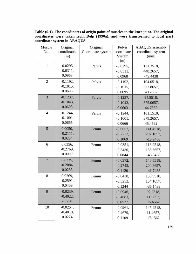
Table (6-1). The coordinates of origin point of muscles in the knee joint. The original coordinates were taken from Delp (1990a), and were transformed to local part coordinate system in ABAQUS.

Muscle No.

Original coordinates

(m)

Original Coordinate system

Pelvis coordinate

System (m)

ABAQUS assembly coordinate system

(mm)

1 -0.0295, -0.0311, 0.0968

Pelvis -0.0295, -0.0311, 0.0968

131.3518, 448.2657, -49.4438

2 -0.1192, -0.1015, 0.0695

Pelvis -0.1192, -0.1015, 0.0695

104.0518, 377.8657, 40.2562

3 -0.1237, -0.1043, 0.0603

Pelvis -0.1237, -0.1043, 0.0603

94.8518, 375.0657, 44.7562

4 -0.1244, -0.1001, 0.0666

Pelvis -0.1244, -0.1001, 0.0666

101.1518, 379.2657, 45.4562

5 0.0050, -0.2111, 0.0234

Femur -0.0657, -0.2772, 0.1069

141.4518, 202.1657, -13.2438

6 0.0356, -0.2769, 0.0009

Femur -0.0351, -0.3430, 0.0844

118.9518, 136.3657, -43.8438

7 0.0335, -0.2084, 0.0285

Femur -0.0372, -0.2745, 0.1120

146.5518, 204.8657, -41.7438

8 0.0269, -0.2591, 0.0409

Femur -0.0438, -0.3252, 0.1244

158.9518, 154.1657, -35.1438

9 -0.0239, -0.4022, -.0258

Femur -0.0946, -0.4683, 0.0577

92.2518, 11.0657, 15.6562

10 -0.0254, -0.4018, 0.0274

Femur -0.0961, -0.4679, 0.1109

145.4518, 11.4657, 17.1562

129

Table (6-2). The coordinates of insertion point of muscles in the knee joint. The original coordinates were taken from Delp (1990a), and were transformed to local part coordinate system in ABAQUS.

Muscle No.

Original coordinates

(m)

Original coordinate

system

Pelvis coordinate System

(m)

ABAQUS assembly

coordinate system (mm)

1 0.0121, 0.0437, -0.0010

Patella -0.0142, -0.4411, 0.0849

119.4518, 38.2657, -64.7438

2 -0.0243, -0.0536, -0.0194

Tibia -0.1003, -0.5157, 0.0641

98.6518, -36.3343, 21.3562

3 -0.0314, -0.0545, -0.0146

Tibia -0.1074, -0.5166, 0.0689

103.4518, -37.2343, 28.4562

4 -0.0081, -0.0729, 0.0423

Tibia -0.0841, -0.5350, 0.1258

160.3518, -55.6343,

5.1562 5 -0.0101,

-0.0725, 0.0406

Tibia -0.0861, -0.5346, 0.1241

158.6518, -55.2343,

7.1562 6 0.0063,

0.0445, -0.0170

Patella -0.0200, -0.4403, 0.0689

103.4518, 39.0657, -58.9438

7 0.0058, 0.0480, -0.0006

Patella -0.0205, -0.4368, 0.0853

119.8518, 42.5657, -58.4438

8 0.0103, 0.0423, 0.0141

Patella -0.0161, -0.4425, 0.1000

134.5518, 36.8657, -62.8438

9 0.0044, 0.0310, -0.0053

Calcanus -0.1203, -0.9031, 0.0861

120.6518, -423.7343,

41.3562 10 0.0044,

0.0310, -0.0053

Calcanus -0.1203, -0.9031, 0.0861

120.6518, -423.7343,

41.3562

130

Table (6-3). The coordinates of the intersection point of muscles line of action and the plate (second and third columns). Data were transferred from assembly coordinate system to plate (local part) coordinate system using MATLAB. The last column contains coordinates of unit vectors to which muscle forces were parallel.

Muscle No. Assembly coordinate system (mm)

Plate coordinate system (mm)

Unit vector

1 120.2306, 65.1000, -63.7424

-11.6324, -5.0000, 44.6141

-0.0290, -0.9989, -0.0373

2 99.9742, 65.1000, 25.9847

78.0947, -5.0000, 64.8705

-0.0130, -0.9989, -0.0456

3 101.3172, 84.6119, 0.0208, 65.1000, -5.0000, -0.9990, 32.5019 63.5275 -0.0395

4 143.9171, 65.1000, 16.3440

68.4540, -5.0000, 20.9276

0.1343, -0.9867, -0.0914

5 150.6108, 49.7292, 0.0665, 65.1000, -5.0000, -0.9947, -2.3808 14.2339 0.0788

6 107.5991, 65.1000, -54.9035

-2.7935, -5.0000, 57.2456

-0.1555, -0.9762, -0.1515

7 123.5589, -4.0151, -0.1615, 65.1000, -5.0000, -0.9817, -56.1251 41.2858 -0.1010

8 140.4249, 65.1000, -56.1764

-4.0664, -5.0000, 24.4198

-0.1984, -0.9539, -0.2253

9 99.1680, -16.8623, -0.0651, -94.8200, 5.0000, 0.9961, 21.9149 13.5885 -0.0589

10 139.3951, -94.8200, 23.0664

-18.0138, 5.0000, 53.8156

0.0568, 0.9968, -0.0554

131

6.2 The Forces of Muscles

The muscle forces create an over-constrained system for the knee joint. An optimization

method is used along with momentum equations to calculate muscle forces (Anderson

and Pandy, 2001). Two optimization methods can be implemented: dynamic optimization

and static optimization. In the first method a forward dynamic approach is used to

determine muscle forces, whereas in the second method an inverse method is used. These

methods give similar results when simulating the gait cycle (Anderson and Pandy, 2001).

In this project the second method was implemented as it is computationally more

efficient (Anderson and Pandy, 2001).

Two sets of equations will be used to determine muscle forces. The first equation

is an optimization criterion which minimizes a function of muscle activations. The

second equation enforces either the simulated angle or the momentum at the knee joint to

be close to the experimentally measured angle or momentum at this joint, as is explained

in the following sections.

6.2.1 Enforcing Angles

The muscle forces are determined so that the calculated angles at the joints are close to

experimentally determined angles within a tolerance. The lower extremity is considered

as a linkage with the hip, the knee and the ankle rotations as its degrees of freedom.

Using the Lagrange method, and considering the motions in the sagittal plane, the

equations of motion for the system are (Piazza and Delp, 1996):

132

2��𝜃 𝐻𝐻 ⎡��𝜃 𝐻𝐻⎤ −��𝜃 𝐻𝐻��𝜃 𝐾𝐾 𝑀𝑀𝐻𝐻⎢ 2 ⎥𝑀𝑀 −��𝜃 𝐾𝐾 = 𝐶𝐶 ⎢��𝜃 𝐾𝐾⎥ + 𝑉𝑉 ��𝜃 𝐻𝐻��𝜃 𝐴𝐴 + 𝐺𝐺 + −𝑀𝑀𝐾𝐾 (6-1) ⎢ ⎥ 𝑀𝑀𝐴𝐴𝜃𝜃𝐴𝐴 ⎣��𝜃 𝐴𝐴

2 ⎦ −𝜃𝜃𝐾𝐾𝜃𝜃𝐴𝐴

In this equation 𝜃𝜃𝐾𝐾 , 𝜃𝜃𝐻𝐻 and 𝜃𝜃𝐴𝐴 are the knee, the hip and the ankle angles, respectively.

Dots are used to refer to time derivatives. One dot represents angular velocity, and two

dots represents angular acceleration. 𝑀𝑀𝐻𝐻, 𝑀𝑀𝐾𝐾 and 𝑀𝑀𝐴𝐴 are the moments produced by

muscles, and matrices 𝑀𝑀, 𝐶𝐶, 𝑉𝑉, and 𝐺𝐺 are related to effects such as inertial and gravity

forces (Piazza and Delp, 1996). The moments at the knee is produced by muscles and

other soft tissues. We assume that the moments caused by other soft tissues is negligible

compared to the moments produced by muscles. This equation can be written in the

following form:

2��𝜃 𝐻𝐻 ⎡𝜃𝜃𝐻𝐻⎤ −��𝜃 𝐻𝐻��𝜃 𝐾𝐾 𝑀𝑀𝐻𝐻⎢ 2 ⎥−��𝜃 𝐾𝐾 = 𝑀𝑀−1𝐶𝐶 ⎢��𝜃 𝐾𝐾⎥ + 𝑀𝑀−1𝑉𝑉 ��𝜃 𝐻𝐻��𝜃 𝐴𝐴 + 𝑀𝑀−1𝐺𝐺 + 𝑀𝑀−1 −𝑀𝑀𝐾𝐾 (6-2) ��𝜃 𝐴𝐴

⎢⎣��𝜃 2 ⎥⎦ −��𝜃 𝐾𝐾��𝜃 𝐴𝐴

𝑀𝑀𝐴𝐴𝐴𝐴

The nonlinear terms in the right-hand side are calculated based on the data from a

previous time step. After this equation is solved, the angular velocity at the knee joint can

be determined once the initial angular velocity is known at this joint, as follows:

𝜏𝜏 𝜏𝜏−∆𝑡𝑡 (6-3)��𝜃 𝐾𝐾 = ∆𝑡𝑡 × ��𝜃 𝐾𝐾 + ��𝜃 𝐾𝐾

And then the angle can be found:

𝜏𝜏 𝜏𝜏−∆𝑡𝑡 (6-4)𝜃𝜃𝐾𝐾 = ∆𝑡𝑡 × ��𝜃 𝐾𝐾 + 𝜃𝜃𝐾𝐾

The knee angle can be calculated for all time steps in a similar manner.

133

On the other hand, the experimentally determined values can be obtained from gait

analysis experiments, as reported in the literature (for example, Perry, 1992, Allard et al.,

1997).

The muscle forces are determined so that:

𝑆𝑆𝑆𝑆𝑚𝑚𝑆𝑆𝑓𝑓𝑎𝑎𝑡𝑡𝑒𝑒𝑆𝑆 − 𝜃𝜃𝐾𝐾 (6-5)𝐸𝐸𝐸𝐸𝑝𝑝𝑒𝑒𝐸𝐸𝑆𝑆𝑚𝑚𝑒𝑒𝐸𝐸𝑡𝑡𝑎𝑎𝑓𝑓 < 𝑇𝑇𝑇𝑇𝑓𝑓𝑒𝑒𝐸𝐸𝑎𝑎𝐸𝐸𝑐𝑐𝑒𝑒 𝜃𝜃𝐾𝐾

6.2.2 Enforcing Moments

In this method, moments resultant from calculated muscle forces are enforced to be close

to experimentally determined joint moments (for example, Perry, 1992, Allard et al.,

1997). Similar to the previous section, we assume the moment at the knee joint is

produced mainly by muscles. In other words, moments produced by other soft tissues is

negligible compared to the moment caused by muscles. The equation used in this section

can be written in the following form:

𝐸𝐸𝐸𝐸𝑝𝑝𝑒𝑒𝐸𝐸𝑆𝑆𝑚𝑚𝑒𝑒𝐸𝐸𝑡𝑡𝑎𝑎𝑓𝑓 < 𝑇𝑇𝑇𝑇𝑓𝑓𝑒𝑒𝐸𝐸𝑎𝑎𝐸𝐸𝑐𝑐𝑒𝑒 𝑆𝑆𝑆𝑆𝑚𝑚𝑆𝑆𝑓𝑓𝑎𝑎𝑡𝑡𝑒𝑒𝑆𝑆 − 𝑀𝑀𝐾𝐾 (6-6)𝑀𝑀𝐾𝐾

𝑆𝑆𝑆𝑆𝑚𝑚𝑆𝑆𝑓𝑓𝑆𝑆𝑆𝑆𝑒𝑒𝑆𝑆 Where 𝑀𝑀𝐾𝐾 , the simulated moment at the knee joint, becomes close to

𝑀𝑀𝐾𝐾𝐸𝐸𝑥𝑥𝐸𝐸𝑒𝑒𝐸𝐸𝑆𝑆𝑚𝑚𝑒𝑒𝐸𝐸𝑆𝑆𝑆𝑆𝑓𝑓 within 𝑇𝑇𝑇𝑇𝑓𝑓𝑒𝑒𝐸𝐸𝑎𝑎𝐸𝐸𝑐𝑐𝑒𝑒. This approach is adopted in this project, and it will be

explained in the next section with more details.

6.3 The Optimization Process

As mentioned earlier, two sets of equations are simultaneously included in the

optimization process. The first equation is the performance criterion as follows:

134

𝐸𝐸

𝐽𝐽 = 𝑎𝑎𝑚𝑚2 (6-7) 𝑚𝑚=1

Where 𝐸𝐸 is the number of muscles, and 𝑎𝑎𝑚𝑚 is the activation of muscle number 𝑚𝑚. From a

physiological point of view function 𝐽𝐽 is related to musculoskeletal endurance.

Musculoskeletal endurance is maximized when 𝐽𝐽 is minimized (Crowninshield and Brand,

1981). The activation of each muscle is bounded to be equal or between 0 and 1:

0 ≤ 𝑎𝑎𝑚𝑚 ≤ 1 (6-8)

The other equation (Eq. 6-6) enforces the calculated moment at the joint be close to the

experimentally measured moment within a tolerance:

𝑆𝑆𝑆𝑆𝑚𝑚𝑆𝑆𝑓𝑓𝑎𝑎𝑡𝑡𝑒𝑒𝑆𝑆 − 𝑀𝑀𝐾𝐾 (6-6)𝐸𝐸𝐸𝐸𝑝𝑝𝑒𝑒𝐸𝐸𝑆𝑆𝑚𝑚𝑒𝑒𝐸𝐸𝑡𝑡𝑎𝑎𝑓𝑓 < 𝑇𝑇𝑇𝑇𝑓𝑓𝑒𝑒𝐸𝐸𝑎𝑎𝐸𝐸𝑐𝑐𝑒𝑒 𝑀𝑀𝐾𝐾

The simulated moment is calculated as follows:

𝐸𝐸 (6-9)𝑆𝑆𝑆𝑆𝑚𝑚𝑆𝑆𝑓𝑓𝑎𝑎𝑡𝑡𝑒𝑒𝑆𝑆 𝑀𝑀𝐾𝐾 = 𝐹𝐹𝑚𝑚 × 𝐸𝐸𝑚𝑚

𝑚𝑚=1

Where 𝐹𝐹𝑚𝑚 and 𝐸𝐸𝑚𝑚 are the force and moment arm for muscle number 𝑚𝑚 about the knee

joint. The moment arms can be calculated from the kinematic data of the knee joint when

the gait cycle is simulated (Delp, 1990b). The formulation to include individual muscle

forces presented in this chapter is general, and it can be used for a gait cycle. However, as

it will explained in the next paragraph, we used 40% gait cycle as an example.

Consequently, in this project, the moment arm data from the literature was used as the

angle of the knee joint was constant. 𝐹𝐹𝑚𝑚 is calculated from muscle activations as follows: 135

0 (6-10)𝐹𝐹𝑚𝑚 = 𝑎𝑎𝑚𝑚 × 𝐹𝐹𝑚𝑚

where 𝐹𝐹𝑚𝑚0 is the maximum isometric force of the muscle number 𝑚𝑚.

The knee joint angle of the current model reconstructed from MRI is almost zero.

On the other hand, the knee joint angle at almost 40% of the gait cycle is zero (Sup et al.,

2008 adopted from Perry, 1992). Consequently, for the analysis of the anatomically

accurate model, only rectus femoris, medial head of gastrocnemius and lateral head of

gastrocnemius were considered. These muscles were included because the forces of

other muscles were almost zero at 40% of the gait cycle (Besier et al., 2009). The

moment arms and maximum isometric forces of these muscles are summarized in Table

(6-4). It should be emphasized that the method to include individual muscle forces

discussed in this chapter can be used for a whole gait cycle, and data for 40% was used as

an example to explain how the method works. The knee moment at 40% gait cycle was

approximated as 20N.m (Sup et al., 2008 adopted from Winter, 1991).

Table (6-4). The moment arm and maximum isometric force of three muscles used in this project (O’Connor 1993, Kellis and Baltzopoulos 1999, Yang et al., 2010).

Muscle Moment arm (m) Maximum isometric force (N)

Rectus femoris 0.0369 854.09 Medial head of gastrocnemius 0.025 1112.2 Lateral head of gastrocnemius 0.025 487.86

6.4 Inclusion of Muscle Forces in the ABAQUS Model

As shown in Fig. 6-2, the anatomically accurate model included distal femur, proximal

tibia and fibula, femoral and tibial cartilages, menisci, and ligaments. This model and the 136

constitutive material behavior of its components were developed by a researcher in our

group (Kazemi, 2013). A plate was created above the femur for the purpose of applying

muscle forces in the model. The Young's modulus of the plate was much higher than

cartilages and menisci (almost rigid). The intersect point of each muscle action line and

the bottom face of the plane was calculated. Three points of the bottom surface of the

plate were obtained in ABAQUS. Assume these points are 𝑎𝑎1, 𝑎𝑎2, 𝑎𝑎3. The origin and

insertion point of each muscle was also calculated in ABAQUS assembly coordinate

system (Tables 6-1 and 6-2). Assume the coordinates of these points for a muscle are

𝑏𝑏1and 𝑏𝑏2. Then the intersect point of the line passing through 𝑏𝑏1and 𝑏𝑏2 and the plate will

be:

−1𝑡𝑡1 𝐸𝐸𝑏𝑏1 − 𝐸𝐸𝑏𝑏2 𝐸𝐸𝑎𝑎2 − 𝐸𝐸𝑎𝑎1 𝐸𝐸𝑎𝑎3 − 𝐸𝐸𝑎𝑎1 𝐸𝐸𝑏𝑏1 − 𝐸𝐸𝑎𝑎1

𝑡𝑡2 = 𝑦𝑦𝑏𝑏1 − 𝑦𝑦𝑏𝑏2

𝑦𝑦𝑎𝑎2 − 𝑦𝑦𝑎𝑎1

𝑦𝑦𝑎𝑎3 − 𝑦𝑦𝑎𝑎1 𝑦𝑦𝑏𝑏1

− 𝑦𝑦𝑎𝑎1 (6-11) 𝑡𝑡3 𝑧𝑧𝑏𝑏1 − 𝑧𝑧𝑏𝑏2 𝑧𝑧𝑎𝑎2 − 𝑧𝑧𝑎𝑎1 𝑧𝑧𝑎𝑎3 − 𝑧𝑧𝑎𝑎1 𝑧𝑧𝑏𝑏1 − 𝑧𝑧𝑎𝑎1

The intersect location of the flowing muscle forces were determined: rectus

femoris, vastus lateralis, vastus medialis, vastus intermedius, short head of biceps

femoris, long head of biceps femoris, semitendinosus, and semimembranosus. Medial

gastrocnemius and lateral gastrocnemius forces were applied at the posterior side of

medial and lateral condyles. The location of the intersecting point of a muscle line and

the plate was calculated in the plate coordinate system after it was found in assembly

coordinate system (Table 6-3). The coordinates of the intersecting point were used to

define a node where the muscle force was applied. The force was applied in the direction

of a unit vector whose components were calculated based on the insertion and origin

point of each muscle (Table 6-3). As it was explained in section 6.3, three muscles rectus

137

femoris, medial head of gastrocnemius and lateral head of gastrocnemius were considered

for the finite element analysis.

1 2 3 4

7 8 5 6

Fig. 6.2: Inclusion of individual muscle forces in an anatomically accurate three-dimensional knee model. The numbers correspond to muscles as follows: 1- vastus lateralis, 2- vastus intermedius, 3-rectus femoris, 4- vastus medialis, 5­semitendinosus, 6- semimembranosus, 7- long head of biceps femoris, 8- short head of biceps femoris. Medial and lateral heads of gastrocnemius forces are applied on the posterior side of femoral condyles. Table (6-3) contains the intersection point coordinates in ABAQUS.

6.5 MATLAB M-files

MATLAB (Mathworks, Natick, Massachusett, USA) programming language was used in

this part of the project. MATLAB codes were used to transfer coordinates between

138

different coordinate systems and also for optimization. These MATLAB files had the

following roles:

- calculations of the components of a unit vector in the direction of each muscle force.

These data were used when a concentrated force was defined for a muscle force in

ABAQUS.

- calculation of the coordinates of the intersection point between a muscle force line of

action and the bottom face of the plate. This location was used to define the location

where the muscle force was applied.

- the transfer of the coordinates of muscle insertion and origin points between different

coordinate systems.

- enforcing the simulated knee moment to be close to the experimental moment (Eq. 6-6).

- calculation of the optimization function (Eq. 6-7).

- optimization of the performance function.

6.6 Results

The model under a 150N compressive load without muscle forces was analyzed. As it

was discussed in section 6.3, the geometry of our model approximately corresponds to

40% of gait cycles. At 40% of the gait cycle, muscles other than rectus femoris, lateral

gastrocnemius, and medial gastrocnemius are almost inactive (Besier et al., 2009).The

muscle forces including rectus femoris, lateral gastrocnemius, and medial gastrocnemius

were then included along with the vertical force to examine the effect of muscle forces on

139

the contact mechanics of the knee joint. Contact pressure at the femoral cartilage is

shown for both cases in Fig. 6.3.

The pattern of contact pressure is the same; however, the contact pressures are

significantly higher when muscle forces are included. The contours would also be

different if the whole gait cycle was considered as the orientation of bones and muscle

forces are considerably altered during different phases of gait. The noticeable effect of

muscle forces on the contact pressure is in line with previous studies that reported the

knee joint is under a much higher burden when muscles are activated (Kuster et al.,

1997).

140

(a)

(b) Fig. 6.3: Contact pressure in the femoral cartilage with (a) and without (b) muscles for approximately 40% of the gait cycle.

141

Chapter Seven: Free-Surface Fluid Pressure

The contact surfaces change as a result of deflections. It is important to adjust the fluid

pressure boundary conditions due to these changes in contact surfaces. As mentioned

earlier, contact surfaces are the interfaces between the femoral cartilage, menisci, and

tibial cartilages. The contact area of each component varies when applied load increases

from zero to a given value.

The models, described so far, assumed no fluid pressure boundary changes during

the solution. The free surfaces were approximated at the beginning of an analysis, and a

node set included in those surfaces was defined. The pore pressure at those nodes was

enforced to be zero during the analysis, as boundary conditions. This method could be

suitable for small knee compressions, but for large knee compressions some of the nodes

which were not in contact initially could become in contact after further deformation.

In this chapter, based on a previous study (Pawaskar et al., 2010), an algorithm is

developed to adjust the free-surface pore pressure as a solution variable. As it will be

explained in the next sections, the pore pressure boundary condition was defined to be

dependent upon contact status, and based on the contact status a seepage coefficient was

used to update the pore pressure at each surface integration point.

142

7.1 Subroutines

To implement the zero fluid pressure condition at the surface two subroutines were used:

FLOW and URDBFIL. The former implements the fluid velocity or fluid pressure

condition at a surface. The latter provides the contact condition of the surface.

7.1.1 FLOW Subroutine

This subroutine uses a seepage coefficient 𝑘𝑘0 and a constant 𝑆𝑆0 (which can be zero) to

enforce the fluid flow condition at a surface. The relation among fluid flow, seepage

coefficient and a reference fluid pressure is:

𝑓𝑓 = 𝑘𝑘0(𝑆𝑆 − 𝑆𝑆0) (7-1)

Where 𝑓𝑓 is fluid velocity in the direction of outward normal to the surface, 𝑘𝑘0 is seepage

coefficient, 𝑆𝑆 is fluid pressure and 𝑆𝑆0 is a reference fluid pressure. If the surface is in

contact with another surface (e.g. two cartilage layers are in contact), and the pore

pressure is equal on both sides of the contact surface, letting k0 be zero will satisfy the

zero velocity condition at the interface. On the other hand, if the surface is free, the fluid

pressure condition should be 𝑆𝑆 = 𝑆𝑆0. This condition will be approximately enforced, if

𝑘𝑘𝑘𝑘0 ≫

𝛾𝛾𝑤𝑤𝑐𝑐 (7-2)

Where 𝑘𝑘 is the permeability of the underlying material, 𝛾𝛾𝑤𝑤 is the specific weight, and 𝑐𝑐 is

the characteristic length of the underlying elements (ABAQUS manual). For standard

geometries (disks and spheres) by two previous studies, 𝑘𝑘0 = 1 𝑚𝑚𝑚𝑚3

was chosen 𝑁𝑁𝑁𝑁

(Pawaskar et al., 2010, Federico et al., 2004, 2005), but our model was not convergent

when that value was used (the base units used are N for force, mm for length and s for

143

time). This could be due to the complexity of the geometry in our model compared to

those studies as well as different element lengths used in our model. When 𝑘𝑘0 =

0.001 𝑚𝑚𝑚𝑚3

was chosen for our model, reasonable results were obtained. According to the 𝑁𝑁𝑁𝑁

ABAQUS manual values of 𝑘𝑘0 set too high might cause “poor conditioning of the

model”, which explains why 𝑘𝑘0 = 1 𝑚𝑚𝑚𝑚3

was not appropriate for our model. In other 𝑁𝑁𝑁𝑁

words, the characteristic seepage coefficient 𝛾𝛾𝑤𝑤

𝑘𝑘

𝑐𝑐 in our model is lower than those in

aforementioned previous models (Pawaskar et al., 2010, Federico et al., 2004, 2005).

The sign of 𝑓𝑓 is another feature that affects the convergence of our model when adjusting

the surface fluid pressure by the method described in this section. When an element is not

in contact, the normal velocity can be outward or inward in respect to the surface. If the

velocity direction is inward, the model will not converge if equation (7-1) is used.

Therefore, the velocity is forced to be zero in that case. In other words, the drainage only

flow is implemented, which corresponds to the non-cyclic loading used in our

simulations.

The FLOW subroutine is activated with 2 command lines in the ABAQUS input file:

*SFLOW

SURFACENAME, QNU

SURFACENAME is the surface name, and QNU is an identifier that tells ABAQUS the

seepage coefficient and a reference fluid pressure will be given for the surface. FLOW

implements Eq. (7-1) at every integration point of the surface. Whether an integration

point is in contact should be determined as the zero fluid pressure was expected to be

144

implemented in non-contacting points. Unfortunately, ABAQUS does not pass the

contact information to this subroutine. As a result, we have to implement an algorithm to

determine if an integration point is in contact or not.

ABAQUS passes the contact pressure at slave surface nodes to URDFIL subroutine, but

ABAQUS does not do so for master surface nodes. Therefore, for a slave surface, the

closest node to an integration point was found. For a master surface, the closest node in

the mating surfaces was found for each integration point. URDFIL was used in both

cases. If the closest node to an integration point was in contact (contact pressure was

larger than zero in the closest node), the pertinent integration point was assumed to be in

contact as well.

7.1.2 URDFIL Subroutine

This subroutine reads the information from the result file. A result file is generated by

ABAQUS if the user requests that in the input file (section 7-2). For example, the nodal

coordinates and pore pressures are written in the result file for a node set called

FEMURE, by the command below:

*NODE FILE, NSET=FEMURE

COORD, POR

The type of written data in the result file depends upon the requests in the input

file. The coordinates of all nodes and also contact pressures in all slave surfaces were

written in the result file in our case. The coordinates of each integration point in the

master surface were known in the FLOW subroutine. As it was explained in section 7.1.1,

145

the code described in this chapter finds the closest node to an integration point and stores

the contact pressure at the node in the memory. As the first step, for each integration

point the contact pressure for the closest node from the previous increment is read. If the

contact pressure is greater than zero, this means the integration point is in contact, and

then the following assignments are done:

= 0 𝑚𝑚𝑚𝑚3

𝑘𝑘0 𝑆𝑆𝑆𝑆

𝑆𝑆0 = 0 𝑀𝑀𝑀𝑀𝑎𝑎 (7-3)

If the contact pressure at the closest node is zero or negative, this means the

integration point is not in contact. In this case, the sign of the velocity component in the

direction of the outward normal to the surface is determined. If that sign is negative, the

adjustments in Eq. (7-3) are done; otherwise, the following assignments are enforced:

= 0.001 𝑚𝑚𝑚𝑚3

𝑘𝑘0 𝑆𝑆𝑆𝑆

𝑆𝑆0 = 0 (7-4)

Figure (7-1) shows this approach for a master surface, in a flowchart format.

146

Read the coordinates of the current integration point

Assume: MINDIS = 2E10

DIS = the distance between current integration point and the next node within the slave surfaces

No DIS > MINDIS

Yes

MINDIS = DIS

No Is this the last node?

𝑓𝑓 < 0

Yes No Yes

Yes

Contact pressure of this node > 0

𝑘𝑘0 = 0, 𝑆𝑆0 = 0 𝑘𝑘0 = 0.001, 𝑆𝑆0 = 0 No

Fig. 7-1: This algorithm is used to distinguish if an integration point in a master surface is in contact or not, and adjust the seepage coefficient accordingly. MINDIS is the distance between the current integration point and the closest node. 𝒌𝒌𝟎𝟎(𝒎𝒎𝒎𝒎

𝟑𝟑)

𝑵𝑵𝑵𝑵 is seepage coefficient, 𝒇𝒇(𝒎𝒎𝒎𝒎 ) is fluid velocity, 𝒖𝒖 is fluid pressure and 𝒖𝒖𝟎𝟎 is a

𝑵𝑵 reference fluid pressure (𝑴𝑴𝑴𝑴𝑴𝑴). "Yeas" means the condition in valid whereas "No" means the condition is not valid.

147

7.2 Result File

The result file must be requested if URDFIL subroutine is used. There is a heading

associated with any type of result data. For instance, the coordinates of nodes is

associated with a heading that specifies the name of the node set for which the

coordinates are written. A key is also associated with any data. For example, pore

pressure is associated with key 108. Results data could be divided into three categories:

integer, real or characters. Arrays “ARRAY” and “JRRAY” contain these data. If the data

is integer or character type “JRRAY” and if the data type is real type, “ARRAY” should

be read. The following example shows how the pore pressure data are written to the result

files, and how they are stored in proper variables in a program.

Data lines to request fluid pressure results in the result file:

NODE FILE, NSET=Femural_Cartilage

POR

Data lines to read and store the number of a node:

INTEGER NODE_NUMBER

NODE_NUMBER = JRRAY(1,2)

Note that node number is the second entry in the JRRAY matrix.

Data lines to read and store the pore pressure of a node:

REAL POR_PRESS

POR_PRESS = ARRAY(4)

Note that pore pressure is the forth entry in the ARRAY vector.

148

7.3 Testing the algorithm

A simple contact model was constructed to test different features of the written code, as

shown in Fig. 7-2. The closest node in the pool of nodes located in the slave surfaces

node set was to be found. To test if the code finds the closest node, a MATLAB program

was also written (Appendix 1). This code was designed to read the coordinates of all

nodes within the slave surface (which was one in this case), and find a node among them,

as close as possible to a given node in the master surface (which was one in this case).

The results obtained from Fortran and MATLAB codes were identical.

Fig. 7-2: A simple model was used to test the algorithm for finding the closest node to an integration point within the master surface.

7.4 Application to the Anatomically Accurate Model

The algorithm was applied on a three-dimensional anatomically accurate model of the

knee joint. For this purpose, no zero fluid pressure boundary condition at the surface was

manually given, but the fluid pressure at the femoral cartilage was defined to be 149

determined according to the algorithm described in section (7-2). The result is shown in

Fig. 7-3. From this figure, we can at least conclude that the algorithm defined the zero

and nonzero fluid pressure zones as expected.

To examine the importance of zero fluid pressure boundary condition at the non-

contact surfaces, another case was studied. In that case, no fluid pressure boundary

conditions were specified for non-contacting surfaces. The resulting fluid pressure is

shown in Fig. 7-4 which is noticeably similar to Fig. 7-3. Even the contour pressures

obtained in Chapters 3, 4, and 5 for the normal model are similar to Figs. 7-3 and 7-4 (see

for example, Fig. 4-2). In Chapters 3, 4, and 5 the fluid pressure at non-contacting

surfaces was implemented by defining a set of nodes, and fluid pressure was manually

enforced to be zero in these nodes. Therefore, a boundary condition to enforce zero fluid

pressure may not affect the results significantly for problems with small simple knee

compression, where the deformation is localized and the contact area does not change

much. However, we indeed need to adjust the boundary conditions per contact conditions

when the knee compression is large or significant sliding and flexion is involved.

150

Fig. 7-3: Surface fluid pressure at the femoral cartilage when the algorithm shown in Fig. 7-1 was used to enforce the fluid pressure boundary conditions (@3s).

151

Fig. 7-4: Surface fluid pressure at the femoral cartilage when no boundary condition was enforced for the free surfaces (@3s).

152

Chapter Eight: Conclusion

8.1 Summary

The effect of normal and pathological properties of articular cartilage on the mechanical

behavior of the human knee joint was studied with emphasize on the fluid pressurization.

Depth-dependent structure and integrity are two of the important features of cartilage.

The hypotheses were: (1) the depth-dependent structure enhances cartilage surface fluid

pressure; (2) a local degeneration in a high load-bearing area in the medial femoral

condyle reduces the surface fluid pressure and the deeper the degeneration is, the more

reduced fluid pressure will be; (3) a local cartilage defect in a high load-bearing area in

the medial femoral condyle reduces fluid pressure and a deeper defect has more

destructive effects on the fluid pressurization. An anatomically accurate finite element

model of the knee joint was constructed using ABAQUS software package to test the

hypotheses.

Depth-dependent properties improved the load bearing capability of the knee

joint. The contribution of fluid pressurization to the applied load significantly reduces the

burden on the solid part of cartilage. Fluid pressurization plays more important roles at

the cartilage surface compared to the deeper zones, as the surface zone has more parallel

collagen fibres. Results showed the depth-dependent properties of cartilage produce

higher surface fluid pressure, supporting our first hypothesis.

Our second hypothesis was also supported. Degenerations leading to advanced

OA could develop from cartilage surface. Advancing layer by layer, degeneration alters

153

the mechanical properties of the tissue including Young's modulus and permeability. As

results showed, degeneration advancement to a layer is associated with decreased fluid

pressure within all other layers including the surface layer. This result implies that the

development of degeneration from the surface facilitates its further development. The

deep cartilage layers close to the cartilage-bone interface experience higher shear strains

as a result of depth-wise advancement of degeneration, increasing the risks of

microfractures occurring at cartilage-bone interface.

The destructive effects due to cartilage defect was also studied using the

anatomically accurate geometry of the knee joint. The effects of cartilage defects on the

knee joint mechanics are more complex compared to cartilage degeneration. Depth-wise

progression of the degeneration was associated with decreased fluid pressure within all

layers, whereas higher fluid pressures were obtained when a defect progressed to the

middle zone of cartilage. Therefore, our third hypothesis was not supported by the results.

8.2 Limitations

A numerical model could be interpreted as a product extracted from a real phenomenon

after simplifying assumptions have been implemented. These simplifying assumptions

cause the major portion of the limitations of any numerical model including the

anatomically accurate normal and pathological models developed in this project. This

section describes the limitations, some of which were discussed in Chapters 3, 4, and 5.

One weak point of the present modelling is the computational time. The analysis

of depth-dependent normal model took almost one week to complete the first second of

154

simulations (loading phase) on a desktop computer with 4 CPUs and 12 GB RAM. When

the number of elements is increased or the loading conditions become more complex the

simulation time increases dramatically. The issue of simulation time becomes more

apparent when the restrictions on the number of ABAQUS licenses are taken into

consideration. Multiple simulations were run in parallel as each one needed a long time to

complete. As a result, too many licenses had to be used simultaneously for long periods,

which was hardly possible using available computational facilities at the University. Due

to long simulation time, local cartilage degeneration (Chapter 4) was modeled for 1s. A

better comparison between effects of degenerations and defects would be possible if the

degenerated case studies were modeled for higher loads as it was done for defects

(Chapter 5).

Simplified loading and boundary conditions are other aspects of the limitations.

Realistic loadings resulting from daily living activities such as gait should be

implemented to make the results more applicable. In this study, however, standard lab

testing loadings including compressive load and displacement were used. Although these

standard loadings provided important insights to the mechanics of the knee joint, some

phenomena will not be seen in the modeling unless loading conditions resembling daily

living activities are considered. For instance, a complex transient loading combined with

forces and moments are applied during a gait cycle in 0.8s. These combined loadings and

their durations have effects on pore pressure, stress, and strain distribution that are not

captured in this project.

155

Lack of experimental validation of the whole knee model is another limitation.

The results from simulations were in line with experimental and numerical reports. The

constitutive model has been extensively validated against experimental measurements (Li

et al., 1999, 2008). Consequently, the results are qualitatively ascertained to reflect the

mechanical behavior of the knee joint in real situations. However, the results would be

more trustworthy if the model is quantitatively validated at the whole joint level.

The sensitivity of the models was not performed for all parameters. The size of

finite element meshes, material properties, fiber orientations, the amplitude and rate of

the loads, boundary conditions, and errors due to the model reconstruction and other

parameters can be altered to investigate how they affect the results. Examples of model

sensitivity analysis can be found in a previous study conducted in our research group

(Kazemi 2013).

The interface between cartilage and bone plays an important role. The current

model assumes the cartilage thickness to be composed of three zones: superficial, middle

and deep zones. Calcified cartilage which is below the deep zone could improve the

accuracy of results when included in a depth-dependent model. This zone of cartilage

becomes more important when the effect of bone stiffness on the mechanics of cartilage

is modeled. The interface between bone and cartilage which includes the calcified zone

significantly influences the development of osteoarthritis (Burr and Radin, 2003, Burr,

2004), but the calcified zone was not modelled in our studies.

Loads, boundary conditions, degeneration area and depth, and defected regions

are altered simultaneously during the development of OA. As a result of this disease, the

156

patient adjusts his/her kinematics and kinetics during activities such as gait (Kaufman et

al., 2001), which means the applied loads and boundary conditions are not constant with

the advancement of OA. Moreover, the areas of degenerated and lost cartilage are

varying with the progression of the disease. However, these changes have not been

considered simultaneously in our studies.

As a last remark, modeling can never be performed without simplifications.

Therefore, limitations will be a part of the model. For example, since the knee joint is one

part of the whole body, another limitation is not to have considered the joint as an

integrated part of the whole body, or at least the lower extremity (Beillas et al., 2004).

8.3 Future Work

Validation of the results obtained for the anatomically accurate model is one of future

directions. Due to the invasive nature of the required procedure, direct in vivo

measurement of parameters such as stress and pore pressure currently seems to be

infeasible. However, measurement of deformation can be performed with medical

imaging. Some measurements can be performed on cadaveric samples and used to

validate the computational results. For instance, contact pressure is a parameter that can

be experimentally measured in cadaveric knee joints using pressure sensors, which could

be compared with computed contact pressures from the model (Papaioannou et al., 2008,

Fukubayashi and Kurosawa, 1980).

Improving the load and boundary conditions according to the kinematics and

kinetics of the lower limb during the gait cycle is a topic of future research. Gait analysis

157

experiments should be conducted to obtain the motions of different joints as well as the

reactions between the ground and the foot. Using inverse dynamics methods, the forces

and moments applied to the knee joint can be calculated (Zajac et al., 2002). These

loading data along with motions obtained for different joints can be used to model the

knee joint mechanics during a whole gait cycle. Modeling the knee joint as a part of a

larger model of the lower extremity will help to implement the loading conditions more

realistically (Beillas et al., 2004). These improvements will deal with challenges such as

numerical difficulties in convergence of the model, high demand in computational

facilities, and problems with capturing the geometry of the lower extremity during a gait

cycle.

The transient nature of muscle forces should be considered in the model as they

vary with time during different activities. The individual muscle forces vary during

different stages of the gait cycle. These forces can be determined according to the

protocol explained in Chapter 6 to model the contact mechanics of the knee joint. Other

activities such as sitting to standing motions, running, or pathological motions such as

gait of below-the-knee amputees can be analyzed to determine kinematic and kinetics of

the lower extremity including muscle forces. These data can then be incorporated in the

finite element anatomically accurate model to get a better understanding about the

development of osteoarthritis in the knee joint.

The depth-dependent structure of cartilage is important when designing artificial

cartilage. Tissue-engineered cartilage might be used as a replacement to biological

cartilage. Knowledge of the structure and properties of cartilage is necessary to design the

158

implanted cartilage so that it mimics the mechanical behavior of native cartilage.

Modeling the depth-dependent structure of cartilage in an anatomically accurate model

provides more accurate results when compared to the case of standard geometries. The

results reported in this thesis could be used as a reference when designing tissue-

engineered cartilage (Ateshian and Hung, 2005).

159

References

Allard P, Cappozzo A, Lundberg A, Vaughan ChL. Three-dimensional analysis of human

locomotion, West Sussex: John Wiley & Sons; 1997.

American Academy of Orthopaedic Surgeons (AAOS). Common Knee Injuries [Online].

Available: http://orthoinfo.aaos.org/topic.cfm?topic=A00325 2007 [Accessed July 6,

2012].

Anderson FC, Pandy MG. Static and dynamic optimization solutions for gait are

practically equivalent. J Biomech 2001;34:153-61.

Ateshian GA, Hung CT. Patellofemoral joint biomechanics and tissue engineering. Clin

Orthop Relat Res 2005;436:81-90.

Athanasiou K, Darling E, and Hu J. Articular cartilage tissue engineering. San Rafael,

Morgan and Claypool Publishers; 2010.

Atkinson PJ, Haut RC. Subfracture insult to the human cadaver patellofemoral joint

produces occult injury. J Orthop Res 1995;13:936-44.

Bagge E, Brooks P. Osteoarthritis in older patients. Optimum treatment. Drugs Aging

1995;7:176-83.

Beillas P, Papaioannou G, Tashman S, Yang KH. A new method to investigate in vivo

knee behavior using a finite element model of the lower limb. J Biomech 2004; 37: 1019­

30.

Bendjaballah MZ, Shirazi-Adi A, Zukor DJ. Biomechanics of the human knee joint in

compression: reconstruction, mesh generation and finite element analysis. Knee

1995;2:69-79.

160

Besier TF, Fredericson M, Gold GE, Beaupré GS, Delp SL. Knee muscle forces during

walking and running in patellofemoral pain patients and pain-free controls. J Biomech

2009;42:898-905.

Biot M. General theory of three-dimensional consolidation. Journal of Applied Physics

1941;12:155-164.

Blankevoort L, Kuiper JH, Huiskes R, Grootenboer HJ. Articular contact in a three-

dimensional model of the knee. J Biomech 1991;24:1019-31.

Burr DB. The importance of subchondral bone in the progression of osteoarthritis. J

Rheumatol Suppl 2004;70:77-80.

Burr DB, Radin EL. Microfractures and microcracks in subchondral bone: are they

relevant to osteoarthrosis? Rheum Dis Clin North Am 2003;29:675-85.

Cailliet R. Knee Pain and Disability. third ed. Philadelphia: F. A. Davis Company; 1992.

p. 70-261.

Carter D, Wong M. Modelling cartilage mechanobiology. Philosophical Transactions of

the Royal Society of London Series B-Biological Sciences 2003;358:1461-71.

Centers for Disease Control and Prevention. Athritis [Online]. Available:

http://www.cdc.gov/arthritis/ 2012 [Accessed July 6, 2012].

Centers for Disease Control and Prevention. Prevalence of self-reported arthritis or

chronic joint symptoms among adults--United States, 2001. MMWR Morb Mortal Wkly

Rep 2002, 51, 948-50.

Cheatham SA, Johnson DL. Current concepts in ACL Injuries. Phys Sportsmed

2010;38:61-8.

161

Crowninshield RD, Brand RA. A physiologically based criterion of muscle force

prediction in locomotion, J Biomech 1981;14:793-801.

Dabiri Y, Najarian S, Eslami MR, Zahedi S, Moser D. A powered prosthetic knee joint

inspired from musculoskeletal system, Biocybern Biomed Eng 2013; 33:118-24.

Delp SL. Surgery simulation: A computer-graphics system to analyze and design

musculoskeletal reconstructions of the lower limb. Stanford University, Ph.D. Thesis,

1990a; p.89-105.

Delp SL. Surgery simulation: A computer-graphics system to analyze and design

musculoskeletal reconstructions of the lower limb. Stanford University, Ph.D. Thesis,

1990b; p.22-4.

Federico S, La Rosa G, Herzog W, and Wu JZ. Effect of fluid boundary conditions on

joint contact mechanics and applications to the modelling of osteoarthritic joints, J

Biomech Eng 2004;126:220–25.

Federico S, Herzog W, and Wu JZ. Erratum: effect of fluid boundary conditions on joint

contact mechanics and applications to the modelling of osteoarthritic joints, J Biomech

Eng 2005;127:208–9.

Felson DT, Zhang Y. An update on the epidemiology of knee and hip osteoarthritis with

a view to prevention. Arthritis Rheum 1998;41:1343-55.

Fukubayashi T, Kurosawa H. The contact area and pressure distribution pattern of the

knee. A study of normal and osteoarthrotic knee joints. Acta Orthop Scand 1980;51:871­

9.

162

Gu K, An anatomically-accurate finite element knee model accounting for fluid pressure

in articular cartilage, the University of Calgary, M.Sc. Thesis, 2010.

Hashemi J, Mansouri H, Chandrashekar N, Slauterbeck JR, Hardy DM, Beynnon BD.

Age, sex, body anthropometry, and ACL size predict the structural properties of the

human anterior cruciate ligament. J Orthop Res 2011;29:993-1001.

Hasler EM, Herzog W, Wu JZ, Müller W, Wyss U. Articular cartilage biomechanics:

theoretical models, material properties, and biosynthetic response. Crit Rev Biomed Eng

1999;27:415-88.

Hayes WC, Keer LM, Herrmann G, Mockros LF. A mathematical analysis for

indentation tests of articular cartilage. J Biomech 1972;5:541-51.

Hughes T. The Finite Element Method. Englewood Cliffs: Prentice-Hall; 1987.

Kaufman KR, Hughes C, Morrey BF, Morrey M, An KN. Gait characteristics of patients

with knee osteoarthritis. J Biomech 2001;34:907-15.

Kazemi M. Finite Element Study of the Healthy and Meniscectomized Knee Joints

Considering Fibril-Reinforced Poromechanical Behaviour for Cartilages and Menisci, the

University of Calgary, Ph.D. Thesis,2013.

Kazemi M, Dabiri Y, Li LP. Recent advances in computational mechanics of the human

knee joint. Comput Math Methods Med 2013;2013:1–27,

http://dx.doi.org/10.1155/2013/718423.

Kellis E, Baltzopoulos V. 1999. In vivo determination of the patella tendon and

hamstrings moment arms in adult males using videofluoroscopy during submaximal knee

extension and flexion. Clin Biomech 1999;14:118–24.

163

Kempson GE, Muir H, Swanson SA, Freeman MA. Correlations between stiffness and

the chemical constituents of cartilage on the human femoral head. Biochim Biophys Acta

1970;215:70-7.

Knecht S, Vanwanseele B, Stüssi E. A review on the mechanical quality of articular

cartilage - implications for the diagnosis of osteoarthritis. Clin Biomech (Bristol, Avon)

2006;21:999-1012.

Korhonen RK, Laasanen MS, Töyräs J, Rieppo J, Hirvonen J, Helminen HJ, Jurvelin JS.

Comparison of the equilibrium response of articular cartilage in unconfined compression,

confined compression and indentation. J Biomech 2002;35:903-9.

Kuster MS, Graeme AW, Stachowiak GW, G chter A. Joint load considerations in total

knee replacemnet. J Bone Joint Surg Br 79;1:109-13.

Larson RL, Grana WA. The knee form, function, pathology, and treatment. Philadelphia:

W.B. Saunders; 1993.

Lawrence RC, Hochberg MC, Kelsey JL, Mcduffie FC, Medsger TA, Felts WR, Shulman

LE. Estimates of the prevalence of selected arthritic and musculoskeletal diseases in the

United States. J Rheumatol 1989;16:427-41.

Lethbridge-Cejku M, Schiller JS, Bernadel L. Summary health statistics for U.S. adults:

National Health Interview Survey, 2002. Vital Health Stat 2004;10:1-151.

Levenston M, Frank E, Grodzinsky A. Variationally derived 3-field finite element

formulations for quasistatic poroelastic analysis of hydrated biological tissues. Computer

Methods in Applied Mechanics and Engineering 1998;156:231-46.

164

Li LP, Herzog W. Strain-rate dependence of cartilage stiffness in unconfined

compression: the role of fibril reinforcement versus tissue volume change in fluid

pressurization, J Biomech 2004; 37: 375–82.

Li LP, Korhonen RK, Iivarinen J, Jurvelin JS, Herzog W. Fluid pressure driven fibril

reinforcement in creep and relaxation tests of articular cartilage. Med Eng Phys

2008;30:182–9.

Li LP, Soulhat J, Buschmann MD, Shirazi-Adl A. Nonlinear analysis of cartilage in

unconfined ramp compression using a fibril reinforced poroelastic model. Clin Biomech

(Bristol, Avon) 1999;14:673-82.

Manek NJ, Lane NE. Osteoarthritis: current concepts in diagnosis and management. Am

Fam Physician 2000;61:1795-804.

Manheimer E, Linde K, Lao L, Bouter LM, Berman BM. Meta-analysis: acupuncture for

osteoarthritis of the knee. Ann Intern Med 2007;146:868-77.

Mansour JM. Biomechanics of cartilage. In: Oatis CA, editors. Kinesiology: the

Mechanics and Pathomechanics of Human Movement. Philadelphia: Lippincott Williams

and Wilkins; 2004. p. 66-79.

Martinez-Villalpando EC, Herr H. Agonist-antagonist active knee prosthesis: a

preliminary study in level-ground walking, J Rehabil Res 2009;46:361-73.

Mononen ME, Mikkola MT, Julkunen P, Ojala R, Nieminen MT, Jurvelin JS, Korhonen

RK. Effect of superficial collagen patterns and fibrillation of femoral articular cartilage

on knee joint mechanics-a 3D finite element analysis. J Biomech 2012;45:579-87.

165

Mow V, Ateshian G. Lubrication and wear of diarthrodial joints. In: Mow V, Hayes W,

editors. Basic orthopaedic biomechanics. second ed. Philadelphia: Lippincott-Raven;

1997. p. 275-316.

Mow VC, Kuei SC, Lai WM, Armstrong CG. Biphasic creep and stress relaxation of

articular cartilage in compression: theory and experiments. J Biomech Eng 1980;102:73­

84.

Mow V, Ratcliffe A. Structure and function of articular cartilage and meniscus. In: Mow

V, Hayes W, editors. Basic orthopaedic biomechanics. second ed. Philadelphia:

Lippincott-Raven; 1997. p. 113-77.

Nordqvist C. What is Arthritis? What Causes Arthritis? [Online]. Available:

http://www.medicalnewstoday.com/articles/7621.php 2009 [Accessed July 6, 2012

2012].

Oliveria SA, Felson DT, Reed JI, Cirillo PA, Walker AM. Incidence of symptomatic

hand, hip, and knee osteoarthritis among patients in a health maintenance organization.

Arthritis Rheum 1995;38:1134-41.

Papaioannou G, Nianios G, Mitrogiannis C, Fyhrie D, Tashman S, Yang KH. Patient-

specific knee joint finite element model validation with high-accuracy kinematics from

biplane dynamic Roentgen stereogrammetric analysis. J Biomech 2008;41:2633-8.

Park S, Hung CT, Ateshian GA. Mechanical response of bovine articular cartilage under

dynamic unconfined compression loading at physiological stress levels. Osteoarthritis

Cartilage 2004;12:65-73.

166

Pauwels F. Biomechanics of the normal and diseased hip. Theoretical foundation.

Techniques and results of treatment, an atlas. Berlin: Springer-Verlag; 1976.

Pawaskar SS, Fisher J, Jin Z. Robust and general method for determining surface fluid

flow boundary conditions in articular cartilage contact mechanics modeling, J Biomech

Eng 2010;132:031001.

Peat G, Mccarney R, Croft P. Knee pain and osteoarthritis in older adults: a review of

community burden and current use of primary health care. Ann Rheum Dis 2001;60:91-7.

Peña E, Calvo B, Martínez MA, Palanca D, Doblaré M. Finite element analysis of the

effect of meniscal tears and meniscectomies on human knee biomechanics. Clin Biomech

(Bristol, Avon) 2005;20:498-507.

Perry J. Gait analysis: normal and pathological function. Thorofare: Slack; 1992.

Piazza SJ, Delp SL. 1996. The influence of muscles on knee flexion during the swing

phase of gait. J Biomech 1996;29:723-33.

Powers CM, Lilley JC, Lee TQ. The effects of axial and multi-plane loading of the

extensor mechanism on the patellofemoral joint. Clin Biomech (Bristol,

Avon) 1998;13:616-624.

Radin EL. Factors influencing the progression of osteoarthritis. In: Ewing J, editors.

Articular cartilage and knee joint function basic science and arthroscopy. New York:

Raven Press; 1990. p. 301-09.

Saarakkala S, Julkunen P, Kiviranta P, Mäkitalo J, Jurvelin JS, Korhonen RK. Depth-

wise progression of osteoarthritis in human articular cartilage: investigation of

composition, structure and biomechanics. Osteoarthritis Cartilage 2010;18:73-81.

167

Saarakkala S, Laasanen MS, Jurvelin JS, Törrönen K, Lammi MJ, Lappalainen R, Töyräs

J. Ultrasound indentation of normal and spontaneously degenerated bovine articular

cartilage. Osteoarthritis Cartilage 2003;11:697-705.

Schinagl RM, Gurskis D, Chen AC, Sah RL. Depth-dependent confined compression

modulus of full-thickness bovine articular cartilage. J Orthop Res 1997;15:499-506.

Shirazi R, Shirazi-Adl A, Hurtig M. Role of cartilage collagen fibrils networks in knee

joint biomechanics under compression. J Biomech 2008;41:3340-8.

Soltz MA, Ateshian GA. Experimental verification and theoretical prediction of cartilage

interstitial fluid pressurization at an impermeable contact interface in confined

compression. J Biomech 1998;31:927-34.

Stoddard S, Jans L, Ripple J, Kraus L. Chartbook on Work and Disability in the United

States. An InfoUse Report. Washington, D.C.: U.S. National Institute on Disability and

Rehabilitation Research 1998.

Sup F, Bohara A, Goldfarb M. Design and control of a powered transfemoral prosthesis.

Int J Robot Res 2008;27:263-73.

Taylor ZA, Miller K. Constitutive modeling of cartilaginous tissues: a review. J Appl

Biomech 2006;22:212-29.

Tsahakis PJ, Brick GW, Thornhill ThS. Arthritis and Arthroplasty. In: Larson RL, Grana

WA, editors. The knee form, function, pathology, and treatment. Philadelphia: W.B.

Saunders; 1993. P. 273-322.

168

Wilson W, Van Donkelaar CC, Van Rietbergen B, Ito K, Huiskes R. Stresses in the local

collagen network of articular cartilage: a poroviscoelastic fibril-reinforced finite element

study. J Biomech 2004;37:357-66.

Winter DA. The Biomechanics and motor control of human gait: normal, elderly and

pathological, second ed. Waterloo: University of Waterloo Press; 1991.

Yang NH, Canavan PK, Nayeb-Hashemi H, Najafi B, Vaziri A. 2010. Protocol for

constructing subject-specific biomechanical models of knee joint. Comput Methods

Biomech Biomed Engin 2010;13:589-603.

Zajac FE, Neptune RR, Kautz SA. Biomechanics and muscle coordination of human

walking. Part I: introduction to concepts, power transfer, dynamics and simulations. Gait

Posture 2002; 16:215-32.

169

Appendix 1: The MATLAB code developed to test the Fortran code for zero fluid pressure boundary condition

function D = testclose()

load the coordinates data of slave surfaces.

for count2 = 1:number of slave surfaces

store the coordinate data of all slave nodes in a matrix.

end

read the coordinates of a master node.

Set the initia guess for the minimum distance.

MINDIS = 5000;

for count1 = 1:number of slave nodes;

store the coordinates of the current slave node in a vector.

Calculate the length of the vector obtained by subtracting the vector of master node

coordinates from the vector of current slave node coordinates (dis);

if(dis < MINDIS)

MINDIS = dis;

row = count1;

end

end

store MINDIS and row

end

170

Appendix 2: The FORTRAN code developed to implement the zero fluid pressure for non-contacting surfaces

SUBROUTINE FLOW(H, SINK, U, KSTEP, KINC, TIME, NOEL, NPT, COORDS,

1 JLTPY, SNAME)

C

INCLUDE 'ABA_PARAM.INC'

C Establish the data in the common block.

COMMON /VECTORS/ V1,V2,V3,V4,V5,V6,V7,V8

C######################################################################

Set a high value for the minimum distance between a master node and a slave node

(MINDIS2).

MINDIS2 = 10e20;

c These are the coordinates of the current integration point.

Read the coordinates of the current integration point (COORDS(1), COORDS(2),

COORDS(3)).

XI = V11(NPT)

YI = V12(NPT)

ZI = V13(NPT)

DO COUNT9=1, 100000 (a number equal to or greater than the number of slave nodes)

Determine the surface to which this slave node belongs, from the common block.

Recall the coordinates of the current slave nodes from common block.

XN = V3(COUNT9)

YN = V4(COUNT9) 171

ZN = V5(COUNT9)

IF this node does not belong to the master surface:

Determine the distance between the current integration point and the current slave node.

DIS2 = SQRT((XI-XN)**2 + (YI-YN)**2 + (ZI-ZN)**2)

IF (MINDIS2.GT.DIS2) THEN

MINDIS2 = DIS2

Store the number of current slave node.

ENDIF

ENDIF

ENDDO

C######################################################################

Read the number of closest node to the current integration point, from previous section.

NEAREST_NODE = V14(NPT)

Read the value of the contact pressure for the nearest node to the current integration

point.

IF (contact pressure.GT.0) Then

Set the appropriate values for seepage coefficient (H) and reference pore pressure (SINK)

H = 0

SINK = 0

ELSEIF (contact pressure.LT.0.OR.contact pressure.EQ.0) THEN

IF (normal outflow velocity.LT.0) THEN

H = 0

172

SINK = 0

ELSE

H= 0.001

SINK=0

ENDIF

ENDIF

ENDIF

RETURN

END

C######################################################################

SUBROUTINE URDFIL(LSTOP, LOVRWRT, KSTEP, KINC, DTIME, TIME)

C

INCLUDE 'ABA_PARAM.INC'

C

DIMENSION ARRAY(513),JRRAY(NPRECD,513),TIME(2)

EQUIVALENCE (ARRAY(1),JRRAY(1,1))

Establish the common block.

COMMON /VECTORS/ V1,V2,V3,V4,V5,V6,V7,V8

C**********************************************************************

DO K1=1, 999999

CALL DBFILE(0, ARRAY, JRCD)

IF (JRCD .NE. 0) GO TO 110

173

KEY = JRRAY(1,2)

IF (KEY.EQ.1503) THEN

KEY 1503 has the information of the name of contacting surfaces.

Store the name of master and slave nodes.

C**********************************************************************

ELSEIF (KEY.EQ.1504.AND. this is the tibial cartilage) THEN

KEY 1504 has the node numbers of contacting surfaces.

Store the number of the current node

ELSEIF (KEY.EQ.1511.AND. this is the tibial cartilage) THEN

KEY 1511 has the contact pressure on a slave node.

ELSEIF (KEY.EQ.1911) THEN

KEY 1911 has the names of node sets.

ELSEIF (KEY.EQ.107.AND.the node set is the tibial cartilage node set) THEN

KEY 107 has the node number and its coordinates.

Store the coordinates of the node.

ELSEIF (KEY.EQ.108.AND.the node set is the tibial cartilage node set) THEN

KEY 108 has the pore pressure at a node.

Store the value of pore pressure at this node

READING DATA OF THE SECOND SLAVE SURFACE (Tibia Cartilages).

IF (KEY.EQ.1504.AND. this is the menisci surface) THEN

KEY 1504 has the node numbers of contacting surfaces.

Store the number of the current node

C

174

ELSEIF (KEY.EQ.1511.AND. this is the menisci surface) THEN

KEY 1511 has the contact pressure on a slave node.

Store the value of contact pressure

ELSEIF (KEY.EQ.107.AND.the node set is the menisci node set) THEN

Store the coordinates of the node.

ELSEIF (KEY.EQ.108.AND.the node set is the menisci node set) THEN

Store the value of pore pressure at this node

C READING DATA OF THE MASTER SURFACE.

IF (KEY.EQ.1504.AND. this is the femoral cartilage surface) THEN

Store the number of the current node

ELSEIF (KEY.EQ.107.AND.the node set is the femoral cartilage node set) THEN

KEY 107 has the node number and its coordinates.

Store the coordinates of the node.

C THE CONTACT PRESSURE IS UPDATED FOR MASTER NODES HERE.

C######################################################################

MINDIS = 10e20;

C These are the coordinates of the current master node.

X1 = COOR1

Y1 = COOR2

Z1 = COOR3

DO COUNT5=1,2000 (a number equal to or greater than the number of all nodes)

IF the current node is not in the femoral cartilage

175

Recall the coordinates of the current slave node from stored data.

Determine the distance between the current slave node and the master node.

DIS = SQRT((X1-X2)**2 + (Y1-Y2)**2 + (Z1-Z2)**2)

IF (MINDIS.GT.DIS) THEN

MINDIS = DIS

Set the contact pressure at the current master node equal to contact pressure at the closest

slave node.

ENDIF

ENDIF

ENDDO

C**********************************************************************

110 CONTINUE

RETURN

END

176

Appendix 3: The Copyright Permission Letter

177

178

179

180

181

Journal and Conference Papers and Abstracts

Journal Papers

Dabiri Y, Li LP. Influences of the depth-dependent material inhomogeneity of articular

cartilage on the fluid pressurization in the human knee. Medical Engineering &

Physics 2013; 35(11), 1591-1598.

Dabiri Y, Li LP. Altered knee joint mechanics in simple compression associated with

early cartilage degeneration. Computational and Mathematical Methods in Medicine

2013; 2013: 1-11, http://dx.doi.org/10.1155/2013/862903.

Dabiri Y, Li LP. Load Bearing Characteristics of the Knee Joint Deteriorates with the

Defect Depth of Articular Cartilage, submitted to Medical & Biological Engineering

& Computing.

Kazemi M, Dabiri Y, Li LP. Recent advances in computational mechanics of the human

knee joint. Comput Math Methods Med 2013; 2013: 1–27,

http://dx.doi.org/10.1155/2013/718423.

Conference Papers and Abstracts

Dabiri Y, Li LP. Comparison of Cartilage Degeneration and Defect on Fluid

Pressurization in the Human Knee, Saskatoon, Canada, June 2-6, 2013.

Dabiri Y, Ahsanizadeh S, Li LP. Effects of the depth of cartilage defect on the knee joint

mechanics: a depth-dependent fiber-reinforced depth-dependent poroelastic model, Salt Lake

City, Utah, USA, April 3-6, 2013.

182

Dabiri Y, and Li LP. A numerical model of mechanics of osteoarthritis in human knee joint,

ASME 2012 International Mechanical Engineering Conference and Exposition, Houston,

Texas, USA, November 9-15, 2012.

Dabiri Y, Li LP. Effect of depth-dependent cartilage properties on cartilage bone interface

mechanics, Canadian Society of Mechanical Engineering, Winnipeg, Canada, June 4-6,

2012.

Dabiri Y, Kazemi M, Li LP. A finite element model of mechanical behaviour of human

knee with osteoarthritis, Canadian Society of Biomechanics, Vancouver, Canada,

June 6-9, 2012.

Dabiri Y, Li LP. The mechanical role of the zonal differences of intact human knee

cartilage, European Society of Biomechanics, Lisbon, Portugal, July 1-4, 2012.

Dabiri Y, Li LP, Mechanical response of human knee joint to sinusoidal compression –

influence of fluid pressurization in soft tissues, ASME summer bioengineering

conference, Puerto Rico, USA, June 20-23, 2012.

Zheng H, Dabiri Y, Kazemi M, Li LP, 3D Knee Joint Reconstruction from MR Images,

12th Alberta biomedical engineering conference, 2011, Banff, Canada, October 21­

23, 2011.

Dabiri Y, Kazemi M, Li LP. Influence of the zonal differences on the mechanics of

articular cartilage in the knee joint. WACBE 5th World Congress on Bioengineering,

Tainan, Republic of China, August 18-21, 2011.

183