the role of different modes of interactions among

Faculty of Environmental Sciences

The role of different modes of interactions among neighbouring plants in driving population dynamics Dissertation for awarding the academic degree Doctor rerum naturalium ( Dr. rer. nat. ) Submitted by M.Sc. Yue Lin Supervisor: Mrs. Prof. Dr. Uta Berger Dresden University of Technology Mr. Prof. Dr. Volker Grimm Helmholtz Centre for Environmental Research – UFZ University of Postdam

Dresden, 22.01.2013

II

Explanation of the doctoral candidate This is to certify that this copy is fully congruent with the original copy of the dissertation with the topic: „ The role of different modes of interactions among neighbouring plants in driving population dynamics “

Dresden, 22.01.2013

……………………………………….….

Place, Date

Lin, Yue

……………………………………….….

Signature (surname, first name)

III

To my doctoral advisors

Prof. Dr. Uta Berger

and Prof. Dr. Volker Grimm

whose wisdoms furnish the best of sounding boards,

whose reliance and optimisms dispel all my misgivings,

whose enthusiasms and professionalisms are contagious,

who welcomed me from China to Germany with open arms,

and who are my mentors forever.

To my dear and loving wife

Qian-Ru Ji

who has made numerous sacrifices to support my studies.

V

Table of contents

Summary ....................................................................................................... VII

Zusammenfassung ......................................................................................... IX

Chapter 1: General introduction ......................................................................1

Chapter 2: Plant competition and metabolic scaling theory ......................... 26

Chapter 3: Mechanisms mediating plant mass-density relationships:

the role of biomass allocation, above- and belowground

competition ............................................................................... 57

Chapter 4: Exploring the interplay between modes of positive and

negative plant interactions ........................................................ 93

Chapter 5: Metabolic scaling theory predicts near ecological equivalence

in plants ................................................................................... 129

Chapter 6: General discussion .................................................................... 139

Acknowledgments ...................................................................................... 151

VII

Summary

The general aim of my dissertation was to investigate the role of plant interactions in

driving population dynamics. Both theoretical and empirical approaches were employed.

All my studies were conducted on the basis of metabolic scaling theory (MST), because

the complex, spatially and temporally varying structures and dynamics of ecological

systems are considered to be largely consequences of biological metabolism. However,

MST did not consider the important role of plant interactions and was found to be invalid

in some environmental conditions. Integrating the effects of plant interactions and

environmental conditions into MST may be essential for reconciling MST with observed

variations in nature. Such integration will improve the development of theory, and will

help us to understand the relationship between individual level process and system level

dynamics.

As a first step, I derived a general ontogenetic growth model for plants which is

based on energy conservation and physiological processes of individual plant. Taking the

mechanistic growth model as basis, I developed three individual-based models (IBMs) to

investigate different topics related to plant population dynamics:

1. I investigated the role of different modes of competition in altering the prediction

of MST on plant self-thinning trajectories. A spatially-explicit individual-based

zone-of-influence (ZOI) model was developed to investigate the hypothesis that MST

may be compatible with the observed variation in plant self-thinning trajectories if

different modes of competition and different resource availabilities are considered. The

simulation results supported my hypothesis that (i) symmetric competition (e.g.

belowground competition) will lead to significantly shallower self-thinning trajectories

than asymmetric competition as predicted by MST; and (ii) individual-level metabolic

processes can predict population-level patterns when surviving plants are barely affected

by local competition, which is more likely to be in the case of asymmetric competition.

2. Recent studies implied that not only plant interactions but also the plastic biomass

allocation to roots or shoots of plants may affect mass-density relationship. To investigate

the relative roles of competition and plastic biomass allocation in altering the

mass-density relationship of plant population, a two-layer ZOI model was used which

VIII

considers allometric biomass allocation to shoots or roots and represents both above- and

belowground competition simultaneously via independent ZOIs. In addition, I also

performed greenhouse experiment to evaluate the model predictions. Both theoretical

model and experiment demonstrated that: plants are able to adjust their biomass

allocation in response to environmental factors, and such adaptive behaviours of

individual plants, however, can alter the relative importance of above- or belowground

competition, thereby affecting plant mass-density relationships at the population level.

Invalid predictions of MST are likely to occur where competition occurs belowground

(symmetric) rather than aboveground (asymmetric).

3. I introduced the new concept of modes of facilitation, i.e. symmetric versus

asymmetric facilitation, and developed an individual-based model to explore how the

interplay between different modes of competition and facilitation changes spatial pattern

formation in plant populations. The study shows that facilitation by itself can play an

important role in promoting plant aggregation independent of other ecological factors (e.g.

seed dispersal, recruitment, and environmental heterogeneity).

In the last part of my study, I went from population level to community level and

explored the possibility of combining MST and unified neutral theory of biodiversity

(UNT). The analysis of extensive data confirms that most plant populations examined are

nearly neutral in the sense of demographic trade-offs, which can mostly be explained by a

simple allometric scaling rule based on MST. This demographic equivalence regarding

birth-death trade-offs between different species and functional groups is consistent with

the assumptions of neutral theory but allows functional differences between species. My

initial study reconciles the debate about whether niche or neutral mechanisms structure

natural communities: the real question should be when and why one of these factors

dominates.

A synthesis of existing theories will strengthen future ecology in theory and

application. All the studies presented in my dissertation showed that the approaches of

individual-based and pattern-oriented modelling are promising to achieve the synthesis.

IX

Zusammenfassung

Das primäre Ziel meiner Dissertation umfasste die Erforschung der Rolle von

Wechselwirkungen zwischen Pflanzen für die Populationsdynamik. Dazu wurden sowohl

theoretische als auch empirische Ansätze angewendet. Alle meine Untersuchungen

wurden auf Basis der Metabolic Scaling Theory (MST) durchgeführt, da angenommen

wird, dass die komplexen räumlich und zeitlich variierenden Strukturen ökologischer

Systeme weitgehend die Konsequenzen von biologischem Metabolismus sind. Allerdings

berücksichtigt die MST nicht die wichtige Rolle der Wechselwirkungen zwischen

Pflanzen und wurde für einige Umweltbedingungen als unzutreffend befunden. Die

Integration dieser Wechselwirkungen und Umweltbedingungen in die MST hingegen ist

essenziell, um die MST mit den beobachteten Abweichungen in der Natur abzustimmen.

Diese Integration wird die Entwicklung von Theorien verbessern und trägt zum

Verständnis der Zusammenhänge zwischen Prozessen auf Individual- und Systemebene

bei.

In einem ersten Schritt leitete ich ein generelles ontogenetisches Wachstumsmodell für

Pflanzen ab, welches auf Energieersparnis und physiologischen Prozessen der

individuellen Pflanzen basiert. Auf dieser Grundlage entwickelte ich drei

individuenbasierte Modelle (IBM), um verschiedene Fragestellungen in Bezug auf die

Populationsdynamik der Pflanzen zu analysieren.

In Kapitel 2 untersuchte ich den Einfluss verschiedener Arten von Konkurrenz auf die

Prognosen der MST in Bezug auf Trajektorien der Selbstausdünnung. Ein räumlich

explizites, individuenbasiertes zone-of-influence (ZOI) Modell wurde entwickelt, um die

Hypothese zu eruieren, dass die MST kompatibel zu den Abweichungen in

Selbstausdünungstrajektorien ist, wenn verschiedene Arten der Konkurrenz und

unterschiedliche Ressourcenverfügbarkeiten in Betracht gezogen werden. Die Ergebnisse

der Simulationen bestätigen meine Hypothese, dass (i) symmetrische Konkurrenz (z.B.:

unterirdisch – Wurzeln) zu signifikant flacheren Selbstausdünnungstrajektorien führt als

bei asymmetrischer Konkurrenz durch die MST vorhergesagt wird; und (ii) metabolische

Prozesse auf Individualebene Muster auf Systemebene vorhersagen können, wenn die

überlebenden Pflanzen kaum durch lokale Konkurrenz beeinflusst werden, was bei

asymmetrischer Konkurrenz meist der Fall ist.

Aktuelle Studien unterstellen, dass nicht nur die Interaktion zwischen Pflanzen, sondern

auch die Biomasseallokation zu Wurzeln oder Trieben der Pflanzen das Masse-Dichte

Verhältnis beeinflussen kann. In Kapitel 3 untersuchte ich die Rolle der Konkurrenz und

Biomasseallokation im Hinblick auf Veränderung des Masse-Dichte Verhältnisses der

Pflanzenpopulation. Dazu wurde ein ZOI Modell mit zwei Ebenen entwickelt, welches

die allometrische Biomasseallokation zu Wurzeln oder Trieben berücksichtigt und sowohl

X

die unter- wie überirdische Konkurrenz durch zwei unabhängige ZOI simultan darstellt.

Zusätzlich führte ich ein Gewächshausexperiment durch, um die Modellprognosen zu

evaluieren. Sowohl das theoretische Modell und das Experiment zeigen, dass Pflanzen in

der Lage sind, ihre Biomasseallokation je nach Umweltfaktoren anzupassen. Diese

individuellen Anpassungsstrategien jedoch verändern die relative Bedeutung der ober-

wie unterirdischen Konkurrenz und damit das Masse-Dichte Verhältnis auf

Populationsebene. Falsche Vorhersagen der MST treten mit höherer Wahrscheinlichkeit

auf, wenn unterirdische Konkurrenz (symmetrisch) vorliegt.

In Kapitel 4 führte ich ein neues Konzept verschiedener Arten der Förderung ein, z.B.:

symmetrische versus asymmetrische Förderung und entwickelte ein individuenbasiertes

Modell um zu ergründen, wie das Zusammenspiel zwischen verschiedenen Arten der

Konkurrenz und Förderung die räumlichen Muster in Pflanzenpopulationen verändert.

Diese Studie zeigt, dass die Förderung allein die Aggregation von Pflanzen maßgeblich

begünstigen kann, unabhängig von anderen ökologischen Faktoren (z.B.:

Samenausbreitung, Mortalität, Heterogenität).

In Kapitel 5 betrachte ich die Ebene der Pflanzengesellschaften und prüfe die

Möglichkeit, die MST mit der Unified Neutral Theory of Biodiversity (UNT) zu

kombinieren. Die Analyse umfangreicher Daten bestätigt, dass die meisten untersuchten

Pflanzenpopulationen nahezu neutral im Sinne des demographischen Trade-off

(Geburt/Sterberate) sind, was durch eine simple Skalierung basierend auf der MST erklärt

werden kann. Dieses demographische Gleichgewicht von Geburt und Mortalität zwischen

verschiedenen Arten und funktionalen Gruppen steht im Einklang mit der Annahme der

Neutral Theory, gestattet jedoch funktionale Abweichungen für manche Arten. Meine

Untersuchung bringt die Debatte darüber, ob Nischen oder neutrale Mechanismen

natürliche Pflanzengesellschaften strukturieren, in Einklang: die eigentlich Frage sollte

lauten, wann und warum einer dieser Faktoren dominiert.

Das abschließende Kapitel 6 beinhaltet eine generelle Diskussion meiner

Untersuchungen und Fragestellungen. Die Synthese bestehender Theorien wird die

Ökologie in Theorie und Anwendung zukünftig stärken. Alle in meiner Dissertation

durchgeführten Untersuchungen zeigten, dass der Ansatz der individuenbasierten und

musterorientierten Modellierung vielversprechend scheint, diese Synthese zu erreichen.

Chapter 1

General introduction

In the mid-19th century, the word ‘ecology’ (Ökologie) was first coined by Ernst

Haeckel in Morphology of Organisms (1866), and was originally defined as the

study of the relationship of organisms with their environment. The environment

of an organism is comprised of all the external factors that could influence it,

including physical and chemical factors (abiotic) or/and other organisms

(biotic). Despite how precise ecology is defined to date (Table 1.1), it is no

doubt that the interactions with those abiotic and biotic factors are fundamental

on the elaboration of ecological theories.

However, some new ecological theories such as the metabolic scaling

theory (MST) attempts at scaling up from the individuals to the ecosystem,

which is based on simple physical rules but overlooks (consciously or

unconsciously) the important role of such interactions. Although claimed to be

a ‘universal’ theory, the validity and universality of MST are still under debate

because some empirical observations in plant populations and communities

are inconsistent with the predictions of MST.

The major goal of my dissertation is to investigate the effects of different

modes of interactions in driving plant population dynamics. All my studies are

under a context of MST, because I am attempted to integrate the effects of

plant interactions and environmental conditions into metabolic scaling theory,

- 2 - Chapter 1

in order to reconcile metabolic scaling theory with observed variations in

nature.

In the following, I will first introduce the field of plant interactions and

then to the overall approach chosen in this thesis, individual-based and

pattern-oriented modelling. Third, I will discuss two ‘unifying’ theories for which

plant interactions play a key role: the Metabolic Scaling Theory and the Unified

Neutral Theory. Finally, I will outline the structure and content of my thesis.

Table 1.1 Textbook definitions of Ecology (after Scheiner and Willig 2008)

Definition Source

The study of the structure and function of nature Odum (1971)

The scientific study of the relationships between organisms

and their environments

McNaughton and

Wolf (1973)

The study of the natural environment, particularly the

interrelationships between organisms and their surroundings

Ricklefs (1979)

The study of animals and plants in relation to their habits and

habitats

Colinvaux (1986)

The study of the relationship between organisms and their

physical and biological environments

Ehrlich and

Roughgarden (1987)

The study of interactions between organisms and between

organisms and their environments

Stiling (1992)

The study of the relationships, distribution, and abundance of

organisms, or groups of organisms, in an environment

Dodson et al. (1998)

The scientific study of the interactions that determine the

distribution and abundance of organisms

Krebs (2001)

The scientific study of the interactions between organisms

and their environment

Begon et al. (2006)

The study of the relationships between living organisms and

their environments, the interactions of organisms with one

another, and the patterns and causes of the abundance and

distribution of organisms in nature

Gurevitch et al.

(2006)

Chapter 1 - 3 -

1.1 Ecology and interactions

1.1.1 Plant competition

In natural situations, the limitation of resources is the crucial issue that links

organisms with their environment. Resource limitation can be caused by both

abiotic and biotic factors. Competition, which per definition is about limiting

resources, is considered perhaps the most important but not the only form of

biotic interactions, which occurs naturally among living organisms that coexist

in same environment. The importance of crop-weed competition was expound

in the ancient Chinese encyclopedia of agriculture The Valuable Techniques

for The Welfare of People (齊民要術, Qí Mín Yào Shù), which had been

completed between A.D. 533 and 544. Although farmers (and agronomists)

were already aware of the importance of competition in managing their

agro-ecosystems long before, the first academic report about competition was

published in the 14th century (Grace and Tilman 1990). Since Darwin (1859),

competition has been established as the conceptual basis for his concept of

‘struggle for life’. Henceforth, most evolutionary biologists view competition as

the main driving force of ‘natural selection’ and, in turn, of evolution. In plant

ecology, the competition is one of the most important topics: it is believed to be

the main force in driving plant phenotype plasticity, life history evolution,

population dynamics, and community assembly (Tilman 1988, Grace and

Tilman 1990).

However, as Grace and Tilman (1990) emphasized in Perspectives on

Plant Competition, although a great deal of research was focused on the topics

of competition for a long time, it is still not well understood. Even the definition

of competition is not consistent. Many ecologists attempted to give an accurate

and unified definition of competition (Milne 1961, Harper 1977, Grime 1979,

Tilman 1988, Begon et al. 2005), but so far, none of them has been generally

accepted. This terminological confusion indicates the complexity of

competition. Begon et al. (2005) defined competition in a very precise way:

- 4 - Chapter 1

“competition is an interaction between individuals, brought about by a shared

requirement for a resource, and leading to a reduction in the survivorship,

growth and/or reproduction of at least some of the competing individuals

concerned”. I advocate using this definition because it gives both the cause

and the consequence of competition, especially when applying in plant

population ecology.

In plant ecology, competition is usually categorized as asymmetric- or

symmetric competition according to the competitive effects (Weiner 1990,

Schwinning and Weiner 1998, Freckleton and Watkinson 2001, Berger et al.

2008). Asymmetric competition is an unequal or disproportional division of

resources amongst competing plants which can be either inter- or intraspecific.

Therefore, competition may be asymmetric in the sense that some species or

individuals have a competitive advantage over others in taking a

disproportionately large amount of resource. The mechanisms determining the

degree of inter- and intraspecific asymmetry are similar: they are

size-dependent and, related to the nature of the limiting resources (Schwinning

and Weiner 1998, Freckleton and Watkinson 2001). For example, taller plants

will have a disproportionate advantage over smaller individuals when

competing for light, because the limiting resource, light, is ‘pre-emptable’. This

can leads to a growth depression of the latter, which has also been referred to

as ‘dominance and suppression’ and ‘one-sided competition’ (Weiner 1990,

Schwinning and Weiner 1998, Stoll et al. 2002, Berger et al. 2008). In contrast,

when the limiting resources are not ‘pre-emptable’ such as water and nutrient,

plants will share resources equally or proportionally to their size (Schwinning

and Weiner 1998, Berger et al. 2008). It is therefore assumed that competition

for light (aboveground competition) is more size asymmetric whereas

competition for water and nutrient (belowground competition) is more size

symmetric (Schwinning and Weiner 1998, Stoll et al. 2002, Berger et al. 2008).

The particular mode of interactions seems to vary depending on

environmental conditions, and whether the interactions occur above- or

Chapter 1 - 5 -

belowground. The latter strongly depends on the type of the shared resources

and their availability. However, due to logistic and technical difficulties, so far

only few studies exist where belowground competition was explored (Morris

2003, Deng et al. 2006, Berger et al. 2008). Most of the empirical experiments

as well as theoretical models only consider light competition as the crucial

process (but see Casper et al. 2003, May et al. 2009, Schiffers et al. 2011). In

heterogeneous or stressful environments, including intra- and interspecific

competition, the relative effect and importance of above- versus belowground

interactions and how they control the structure and function of populations and

communities are still poorly understood (Berger et al. 2008).

In view of its complexity, ecologists have intensely debated the

relevance of different aspects of competition to particular theories. There is

one debate on the prevalence and importance of competition along

environmental gradient which is commonly mentioned as two opposite theories

of competition, and is usually associated with two of its main protagonists,

Grime and Tilman (for a summary, see e.g. Goldberg et al. 1999, Brooker et al.

2005). One view point suggested that plant competition is more dominant

within plant systems in productive and mild environments, but the role of

competition played within plant systems will decreases when productivity

decreases and environmental gradient increases (Grime 1979, Huston 1979,

Keddy 1989). The opposite view point is that competition is predominant within

plant systems irrespective of system productivity or environmental stress,

while the mechanisms by which plants compete can vary, namely, plants

compete strongly for light or space in productive and mild environments, while

in unproductive and harsh environments plants compete mainly for water or

soil nutrients (Newman 1973, Tilman 1982, 1987, 1988, Grubb 1985). Both

points of view have been supported by empirical evidences, and were

considered to be irreconcilable at their fundamental assumptions.

Grace (1991) pointed out that this debate was primarily aggravated by a

failure of distinguishing between two components of competition, the

- 6 - Chapter 1

‘importance’ and ‘intensity’ of competition. The differences between those two

concepts are explicitly (Welden and Slauson 1986): The intensity of

competition is the absolute impact, which relates directly to the physiological

aspects of individuals, but indirectly and conditionally to their fitness, as well as

the dynamics of populations and the structure of communities. The importance

of competition is also not necessarily correlated with the intensities of other

ecological processes. In contrast, the importance of competition is its impact

relative to the environmental factors that influence individual success, which

relates indirectly to their physiological aspects but directly to the ecology and

fitness of individuals. The importance of competition is necessarily relative to

the importance of other ecological processes. Furthermore, intensity refers to

the impact of present competition on individuals, whereas importance refers to

the products and consequences of past competition on individuals and

possibly the systems.

Although it has been argued that Tilman’s theory concerns intensity

whereas Grime’s theory more emphasize importance (see e.g. Grace 1991),

the concept of importance is still frequently neglected. Such widespread

confusion between intensity and importance also arise within studies of plant

positive interactions (Brooker et al. 2005, Brooker and Kikvidze 2008), and

becomes a barrier to our understandings about the role of interactions may

play in plant populations and communities.

1.1.2 Plant facilitation

Over the last decade or so, the role of plant positive interactions has received

increasing attention and is now widely recognized in both empirical and

theoretical ecology (Bertness and Callaway 1994, Brooker et al. 2008,

Bronstein 2009, Maestre et al. 2009). In plant ecology, positive interactions are

usually referred to as facilitation, which I define here as: the interaction

between individual plants via moderation of biotic and abiotic stress,

Chapter 1 - 7 -

enrichment of resource or increased access to resource, which leads to an

increase in the survivorship, growth and/or reproduction of at least some of the

interacting individuals involved. This definition of facilitation is complementary

to the definition of competition given by Begon et al. (2005; see above).

Facilitation seems to be particularly important under harsh

environmental conditions, i.e. abiotic stress. The ‘stress gradient hypothesis’

(SGH) proposes that competition and facilitation may act simultaneously, but

the relative importance of facilitation and competition will vary inversely along

gradients of physical stress. Under high stress conditions, facilitation should be

dominant over competition in shaping of community structures (Bertness and

Callaway 1994, Brooker et al. 2008, Maestre et al. 2009). The SGH has been

supported by many studies: the interplay between facilitation and competition

can drive population dynamics (Chu et al. 2008, 2009, 2010, McIntire and

Fajardo 2011), community structure (Gross 2008, Xiao et al. 2009), community

diversity (Cavieres and Badano 2009), ecosystem functions (Callaway et al.

2002, Kikvidze et al. 2005), and evolutionary consequences (Bronstein 2009,

McIntire and Fajardo 2011). However, there are also studies which do not

support SGH predictions, as facilitative effects have not been detected in some

extreme stress situations (Tielbörger and Kadmon 2000, Maestre et al. 2005,

2009). The mechanistic explanations for SGH as well as facilitation are not

well presented. This indicates that the conceptual framework underlying the

SGH might need further refinement (Maestre et al. 2009). And in fact, whereas

numerous studies exist that explore the consequences of different modes of

competition, i.e. symmetric versus asymmetric competition (Schwinning and

Weiner 1998, Weiner et al. 2001, Stoll and Bergius 2005, Berger et al. 2008),

so far different modes of facilitation have not been well explored. Inconsistent

definitions of facilitation and the lack of differentiation between the impacts of

plant-plant interactions on beneficiary and benefactor individuals have recently

been identified as important gaps in current research (Brooker et al. 2008,

Bronstein 2009, Brooker and Callaway 2009, Pakeman et al. 2009). Refining

- 8 - Chapter 1

and clarifying the concept of facilitation is crucial for understanding how

facilitation arises, persists and evolves.

1.1.3 The interplay between negative and positive interactions

Theoretically, there are three fundamental forms of interaction between

two individuals (species): neutral (0), positive (+) and negative (−). According

to different definitions, modes of facilitation can be mutualistic (+/+),

commensal (+/0) or even antagonistic (+/−) among plants (Brooker et al. 2008,

Bronstein 2009). If competition and facilitation occur at the same time, there

are six possible combinations: −/−, 0/0, +/+, −/0, +/0 and −/+. Considering the

facts that when individuals are together or apart show different modes of

interaction, the possible combinations could increase to 10 (Table 1.2).

However, an approach which incorporates the existing definitions of both

competition and facilitation as special cases might be more useful. Thus, it is

efficient to completely transfer, albeit conversely, the concept of modes of

competition to the new concept of modes of facilitation (Table 1.2). This new

conceptual model has three advantages: first, it is analogous, and therefore

directly comparable to the widely used and important concept of symmetric

and asymmetric interaction (Schwinning and Weiner 1998, Weiner et al. 2001,

Stoll and Bergius 2005, Berger et al. 2008); second, it offers a quantitative and

operational means of evaluating both competitive and facilitative impacts; and

last, it can help us to integrate the facilitation with competition theories

(Callaway et al. 2002, Berger et al. 2008, Brooker et al. 2008, Bronstein 2009,

Maestre et al. 2009).

Chapter 1 - 9 -

Table 1.2 Modes of interactions among two individuals (or species) (A and B).

Defined according to the effect of this interaction for each organism (positive +,

negative −, or no effect 0). A: asymmetric; S: symmetric; C: competition; F: facilitation.

Forms of interaction Together Apart Possible combinations of

the modes of interaction A B A B

Neutralism 0 0 0 0 Neutrality or SC + SF

Competition − − 0 0 SC

Amensalism 0 − 0 0 AC

Parasitism + − − 0 AC + AF

Commensalism + 0 − 0 AF

Mutualism + + − − SF

Unnamed + + 0 − SF or AF

Proto-cooperation + + 0 0 SF

Unnamed + − 0 0 AC + AF

Unnamed + 0 0 0 AF

- 10 - Chapter 1

1.2 Ecology, individual-based models and pattern-oriented

modelling

A main goal of ecology as a science is to understand the interactions of

organisms among themselves and their environment. Individual-based models

(IBMs, or also known as agent-based models ABMs in social science) are thus

a natural tool for ecology because IBMs are capable of taking into account

local interactions, individual variability, adaptive behaviour, environmental

heterogeneous, abiotic stress, disturbance and other ecological factors

(DeAngelis and Gross 1992, Grimm 1999, Grimm and Railsback 2005, Grimm

et al. 2005, Berger et al. 2008).

A model is a simplified version of the real world only dealing with a

limited number of factors which are considered most relevant. Ecological

models attempt to capture the essences of ecological system for addressing

specific questions about the given system (Grimm and Railsback 2005). The

systems of interest in ecology are usually made up of myriad interacting

organisms. Organisms are so different from each other, interacting with others

and physical environment in their unique ways. Grimm and Railsback (2005)

argued that ecology and biology are still lacking in strong mathematical tools to

understand and predict such individual-based complex systems.

With the development of computer science, bottom-up simulation

modelling approaches have been developed a lot in ecology. Using bottom-up

approaches, ecologists compile relevant information at a lower level of the

system, formulate and implement rules about individual’s behaviour in a

computer simulation, and then observe and understand the emergence of

properties related to particular questions at a higher level of integration (Grimm

et al. 2005). In particular, individual-based modelling follows the bottom-up

framework and helped in understanding emergent properties of complex

systems such as population dynamics or community assembly out of the

ecological traits, behaviours and interactions of individual organisms

Chapter 1 - 11 -

(DeAngelis and Gross 1992, Breckling et al. 2005, Grimm and Railsback

2005).

In plant ecology, individual-based approaches are widely used for

modelling plant interactions (Czárán 1997, Berger et al. 2008). In a recent

review, Berger et al. (2008) comprehensively compared different approaches.

Based on Berger et al.’s classification, there are three important approaches

which I think are most advisable: cellular automaton (CA, or the so called

grid-based models), zone-of-influence (ZOI), and field-of-neighbourhood (FON)

(Berger and Hildenbrandt 2000, 2003, Berger et al. 2004). These approaches,

from simple to more sophisticated, have their advantages and limitations and

should be applied to different research questions accordingly (see Berger et al.

2008 for details). However, existing modelling approaches for investigating

plant interactions show three major gaps. New approaches are needed that: (i)

help understanding the mechanisms of plants’ development and response to

their local environment, (ii) consider plants’ adaptations to changing

environmental conditions, and (iii) simultaneously consider positive and

negative interactions among neighbouring plants as well as above- and

belowground interactions.

Modelers greatly rely on the principle of parsimony in developing

models, known as the ‘Occam’s razor’. However, the Occam‘s razor should be

use appropriately in individual-based modelling, because the relationship

between a model’s complexity and payoff is no longer monotonically negative

(as assumed for classical models), but really a hump-shape (Fig 1.1). John

Holland (1995) had formulated this as “Model building is the art of selecting

those aspects of a process that are relevant to the question being asked”. His

interpretation not only highlights the principle of parsimony, but also highlights

that the question being asked is the element of the scientific problem that

should be referenced to determine the components of a model.

- 12 - Chapter 1

Fig. 1.1 A model’s payoff (in terms of how much we can learn from it) versus its

complexity (after Grimm and Railsback 2005). In contrast to analytical models of

classical theoretical ecology (dashed line), where payoff is high only for very simple

models and then declines continuously with complexity, IBMs and other bottom-up

simulation models (humped curve) have a “Medawar zone” at intermediate complexity

where payoff is maximized.

IBMs should be neither too simple nor too complex if they are to be

useful (Grimm and Railsback 2005). To make the bottom-up modelling and

individual-based modelling more rigorous and comprehensive, a strategy

named pattern oriented modelling (POM) was developed (Grimm et al. 1996,

2005, Wiegand et al. 2003, Grimm and Railsback 2005). Because patterns are

the observations of any kind showing specialized, sustained, repeated and

nonrandom characteristics of the system, which contain information on the

mechanisms how they emerge from lower level and the essential structures

and processes, therefore could be used to guide model design (Grimm et al.

1996, 2005, Wiegand et al. 2003, Grimm and Railsback 2005).

The protocol of POM includes four steps (Wiegand et al. 2003, Grimm

and Railsback 2005, Piou 2007): (1) “aggregation of individual based biological

information” for model construction, (2) “determination of parameter values”, (3)

Chapter 1 - 13 -

“systematic comparison between the observed pattern and the simulated

pattern produced by the model” for model evaluation, and (4) “secondary

predictions”. The steps (1) and (2) ensure that properties or patterns at higher

levels emerge from lower-level information incorporated in IBMs. The steps (3)

and (4) leading to the increase in reliability of the IBMs. In this sense, POM is

useful not just for individual-based modelling, but for any kind of modelling. In

addition, POM can also be used to test and refine theory, and can help to

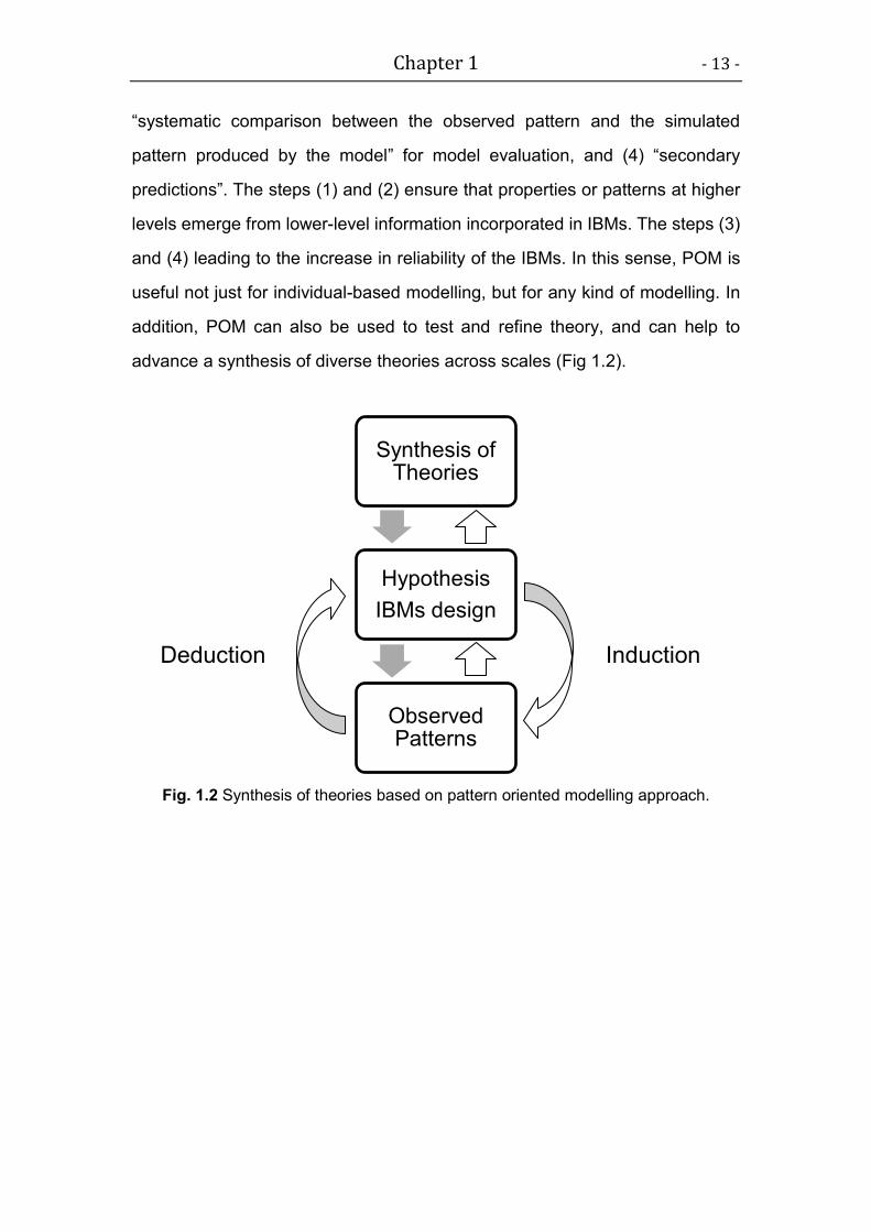
advance a synthesis of diverse theories across scales (Fig 1.2).

Fig. 1.2 Synthesis of theories based on pattern oriented modelling approach.

Synthesis of Theories

Hypothesis

IBMs design

Observed Patterns

Deduction Induction

- 14 - Chapter 1

1.3 Are there universal laws or unified theories in ecology?

More than a decade ago, John Lawton (1999) wrote that, “Parts of science,

areas of physics for instance, have deep universal laws, and ecology is deeply

envious because it does not”. This kind of discontent is perhaps driven by a

fact that use of the laws and models in ecology are usually very local and

highly contingent, and the system studied in ecology are too complex and

contingent to apply the general laws and models.

However, this pessimism regarding a theoretical foundation of ecology

represents a misplaced ‘physical envy’ (Cohen 1971). It is misplaced on at

least two aspects: first, in ecology, the building blocks of systems are living

organisms not particles (Grimm and Railsback 2005). Open a bottle of perfume

in a closed room, the liquid of perfume will become a smelly cloud and fills up

the room eventually, which is state by the second law of thermodynamics.

However, organisms try their best to avoid this smelly cloud of equilibrium,

they can reproduce, interacting with others and environment, seeking fitness,

acquiring resources to maintain internal order and build complexity by

exporting entropy. Erwin Schrödinger (1944) also pondered these questions

and described the negative entropy among organisms: “The essential thing in

metabolism is that the organism succeeds in freeing itself from all the entropy it

cannot help producing while alive”. It is metabolism that makes living

organisms to be unique creatures. Second, the laws of physics are all ‘ceteris

paribus’ laws assumed in ideal vacuums, but the actual governance of, for

instance, particle movement is much more complicated than these general

laws would imply (Cartwright 1983, Simberloff 2004). Therefore, ecology

cannot and should not just try and copy physics.

Over the last decade, several new theories emerged which address the

core principles of ecology, such as Metabolic scaling theory (Brown et al.

2004), Neutral theory in ecology (Hubbell 2001), Ecological stoichiometry

(Sterner and Elser 2002), Maximum entropy of ecology (Harte 2011), Dynamic

Chapter 1 - 15 -

energy budget theory (Kooijman 2009), etc., all having their advantages and

shortages but claiming to be the ‘general’, ‘universal’ or ‘unified’ theory. There

are two striking theories (Gaston and Chown 2005), which attract me most

among all those theories. The first one is Metabolic Scaling Theory (MST)

(also named as Metabolic theory of ecology, Brown et al. 2004), which is an

attempt to link physiological processes of individual organisms with

macroecology. Based on a fractal model of circulatory networks, such as the

vascular system in animals and plants, MST predicts how metabolic rate

increases with body size and temperature following a quarter-power scaling

law. This simple scaling law has been observed from intracellular levels to

individual levels of mammals, covering 27 orders of magnitude (West and

Brown 2005), this even more than the span between earth and whole galaxy

(18 orders of magnitude). Consequently, a large numbers of studies have

explored the ecological consequences of scaling relationships between

organism body size and developmental time, reproduction, population energy

use, abundance, population demographic rate, community structure and

species diversity. Many of these studies were published in high-profile journals

which reflect the promise and potential significance of such a general theory.

However, like any other claim for a ‘universal’ theory, MST has also

generated controversy. For instance, MST predicts a ‘-4/3 universal scaling

law’ for plant mean mass-density relationships (Enquist et al. 1998), but

empirical observations are more variable. Empirical evidences from harsh

areas or from plantation experiments with low resource levels often deviate

from these predictions and show significantly less negative exponents, i.e.

shallower slopes of the self-thinning trajectory or log mass-log density

relationship, respectively (Morris 2003, Deng et al. 2006, Liu et al. 2006).

Consequently, both the validity and universality of scaling exponents and MST

are still unclear and require further analyses of the underlying mechanisms

(Coomes 2006, Deng et al. 2006, Coomes et al. 2011).

- 16 - Chapter 1

A core assumption of MST is that the processes internal to individuals

determine mass-density relationships, whereas interactions among individuals

are largely ignored. Therefore, population dynamic and community assembly

in MST are just a spatial packing process (Reynolds and Ford 2005). An

alternative view is that internal mechanism may play an important role and set

limits on mass-density relationships, but that ecological interactions can be

more important in determining the relationships in the field. Thus, variation in

the ecological conditions and the interactions among individuals can explain

the observed variation in scaling exponents. Specifically, it has been argued

that competition among plants will change mass-density relationships from

those predicted by MST (Coomes et al. 2011).

The second significant theory recently development in ecology is the

Unified Neutral Theory of biodiversity and biogeography (UNT) (Hubbell 2001).

UNT is based on a seemingly unrealistic assumption of ecological equivalence,

that all individuals are functionally equivalent on a per capita basis, i.e. with

respect to their birth, death, dispersal and speciation. Even so, it successfully

explains many patterns about the relative species abundance across different

communities (Hubbell 2001, Chave 2004, Gaston and Chown 2005). UNT

emphasizes ecological drift, dispersal and speciation as the main drivers of

community assembly, thus the abundance of individuals of all species should

be a ‘martingale’ in communities. It severely bucks the basis of ecology by

leaving niche differences and, hence, selection out.

Not surprisingly, criticism in this theory has been predominantly directed

at the fundamental assumption of neutrality. Hubbell (Hubbell 2001, 2005,

2006, 2008) argue that even though the equivalence assumption is not

apposite, the neutral model heavily relies on the principle of parsimony and

predicts real patterns in nature, therefore should not be misjudged. However,

in a POM view, the neutral model is located apparently on left side of the

‘Medawar zone’. It is too simple hence fails in reality and justification that

species are apparently different in varied aspects, and some details on the

Chapter 1 - 17 -

assumption are needed. Indeed, the neutral model stimulated ecologists to

revise the equivalence assumption. Some researchers relaxed the strict

neutrality assumption by considering fitness equivalence via ecological

trade-offs (K. Lin et al. 2009). Their modified neutral models clearly showed

that birth-death trade-offs can lead to a similar result as strict neutral model did.

However, the mechanisms underlying this demographic trade-off are still

unknown.

As Simon Levin (2000) laid out, “the most important challenge for

ecologists remains to understand the linkages between what is going on at the

level of the physiology and behaviour of individual organisms and emergent

properties such as the productivity and resiliency of ecosystems”. Both MST

and UNT or similar theories that are based on simple physical rules attempt to

scale up from the individual to the system. Predictions made by those theories

sometimes become invalid in nature because macroscopic features of the

system can emerge from the large numbers of interacting individual organisms.

Individual-based ecology, with IBM and POM (Grimm and Railsback 2005,

Grimm et al. 2005), I believe, can help us to ultimately achieve a synthesis of

theories in ecology which focus on different processes, organization levels, or

scales.

- 18 - Chapter 1

1.4 Objectives and content of the dissertation

My major goal in this dissertation is to investigate the effects of different modes

of interactions in driving plant population dynamics. Specifically, I explored the

relative role of asymmetric- versus symmetric competition, above- versus

belowground competition, and negative versus positive interactions in shaping

plant population along the environmental gradients by using spatially-explicit

individual-based models. The pattern-oriented modelling approach is applied

in my individual-based modelling studies. Some of the model predictions are

tested with greenhouse experiments and field studies. Although my studies in

this dissertation are mostly on mono-population dynamics, the models and

theories presented are general, so that in principle they can be extended to

communities. All my studies are under a context of metabolic scaling theory

(MST), because I am attempted to integrate the effects of plant interactions

and environmental conditions into metabolic scaling theory, in order to

reconcile metabolic scaling theory with observed variations in nature.

First of all, I derived a general ontogenetic growth model for vascular

plants which is based on energy conservation and physiological process of

individual plant (see Appendix A in Chapter 2). This new mechanistic model is

thus different from the phenomenological growth models which are generally

used in individual-based models of plant interactions. Some extensions and

predictions based on the new growth model are tested by empirical data. My

individual-based simulation models are developed on the basis of this general

growth model.

In Chapter 2, I present a generic spatially-explicit individual-based

model, which I named as pi (plant interaction) model. The pi model implements

different modes of competition (from completely asymmetric to completely

symmetric) among individual plants via their overlapping zone-of-influence

(ZOI). I used the ZOI approach because it is easy to implement and to

combine with metabolic scaling theory. The pi model was used here to

Chapter 1 - 19 -

investigate the hypothesis that MST may be compatible with the observed

variation in plant self-thinning trajectories if different modes of competition and

different resource availabilities are considered. Specifically, two hypotheses

were investigated by using a one-layer ZOI model: (1) if surviving plants are

not highly affected by local interactions, then individual-level metabolic

processes can predict population-level mass-density relationships; and (2)

size-symmetric competition (e.g. belowground competition) will lead to

shallower self-thinning trajectories.

Recent studies on plant competition and MST imply that not only plant

interactions (Coomes et al. 2011, Rüger and Condit 2012) but also the plastic

biomass allocation to roots or shoots of plant can affect mass-density

relationship (Morris 2003, Deng et al. 2006, Zhang et al. 2011). However, the

relative roles of those two factors, competition and plastic biomass allocation,

are still unknown. In Chapter 3, both a theoretical model and an experiment

are used to answer this question. Since the one-layer pi model is too simple,

though, to explore the relative role of plasticity of biomass allocation and

below- versus aboveground competition, I developed a new two-layer model

which represents both above- and belowground competition simultaneously

via independent ZOIs. In the tow-layer pi model, plant growth and biomass

allocation are represented by the growth function based on MST (Enquist 2002,

Niklas 2005, Lin et al. 2012), which tries to mechanistically capture the plastic

responses of plants to changing environmental conditions. In addition, a

greenhouse experiment with tree seedlings is employed to evaluate the

behaviour of the simulated plants related to the allocation patterns and to

validate our model predictions regarding the mass-density relationship.

Specifically, I focus on the following research questions: (1) how does plant

phenotype plasticity (root/shoot biomass allocation in heterogeneous

environments) affect emergent patterns observed at the system level (e.g.,

variation of plant mass-density relationship)? (2) What are the resulting effects

- 20 - Chapter 1

of above- and belowground competition modified by plants’ morphological

adaptations to environmental severity on population dynamics?

In Chapter 4, the effects of both negative and positive plant interactions

on population spatial dynamics are investigated. I introduce a new concept of

symmetric vs. asymmetric facilitation and present the modified pi model. This

new model is able to simultaneously implements different modes of both

facilitation and competition among individual plants. Because different modes

of facilitation are considered as a continuum related to the environment, I

explored this concept within the context of the stress gradient hypothesis

(Bertness and Callaway 1994, Brooker et al. 2008). Specifically, I address the

following questions at both the plant population and individual levels: (1) How

does the interplay of different modes of competition and facilitation change

spatial pattern formation during self-thinning in conspecific cohorts that initially

have a random or aggregated distribution; and (2) How do combinations of

modes of competition and facilitation alter the intensity of local plant

interactions along a stress gradient?

In Chapter 5, I attempt to combine neutral theory and metabolic scaling

theory. Demographic equivalence regarding birth-death trade-offs between

different species is consistent with the assumption of neutral theory but allows

differences between species as suggested by niche theory (Lin et al. 2009).

Based on MST, I deduced an allometric scaling rule which can explain

observed demographic trade-offs. In this preliminary study, I tested the validity

of deduced demographic trade-off by a broad array of plant species. The

ultimately aim of my study is the synthesis of existing theories to strengthen

future ecology in theory and application.

The concluding Chapter 6 offers the general discussion and outlook

related to my study topics. An opinionated review about the development of

theories in ecology is also presented.

Chapter 1 - 21 -

References

Begon, M., C. R. Townsend, and J. L. Harper. 2005. Ecology: From Individuals to

Ecosystems. John Wiley & Sons.

Berger, U., and H. Hildenbrandt. 2000. A new approach to spatially explicit modelling of

forest dynamics: spacing, ageing and neighbourhood competition of mangrove trees.

Ecological Modelling 132:287–302.

Berger, U., and H. Hildenbrandt. 2003. The strength of competition among individual trees

and the biomass-density trajectories of the cohort. Plant Ecology 167:89–96.

Berger, U., H. Hildenbrandt, and V. Grimm. 2004. Age‐related decline in forest

production: modelling the effects of growth limitation, neighbourhood competition and

self‐thinning. Journal of Ecology 92:846–853.

Berger, U., C. Piou, K. Schiffers, and V. Grimm. 2008. Competition among plants:

concepts, individual-based modelling approaches, and a proposal for a future

research strategy. Perspectives in Plant Ecology, Evolution and Systematics

9:121–135.

Bertness, M. D., and R. Callaway. 1994. Positive interactions in communities. Trends in

Ecology & Evolution 9:191–193.

Breckling, B., F. Müller, H. Reuter, F. Hölker, and O. Fränzle. 2005. Emergent properties

in individual-based ecological models—introducing case studies in an ecosystem

research context. Ecological Modelling 186:376–388.

Bronstein, J. L. 2009. The evolution of facilitation and mutualism. Journal of Ecology

97:1160–1170.

Brooker, R., Z. Kikvidze, F. I. Pugnaire, R. M. Callaway, P. Choler, C. J. Lortie, and R.

Michalet. 2005. The importance of importance. Oikos 109:63–70.

Brooker, R. W., and R. M. Callaway. 2009. Facilitation in the conceptual melting pot.

Journal of Ecology 97:1117–1120.

Brooker, R. W., and Z. Kikvidze. 2008. Importance: an overlooked concept in plant

interaction research. Journal of Ecology 96:703–708.

Brooker, R. W., F. T. Maestre, R. M. Callaway, C. L. Lortie, L. A. Cavieres, G. Kunstler, P.

Liancourt, K. Tielb rger, J. M. . Travis, and F. Anthelme. 2008. Facilitation in plant

communities: the past, the present, and the future. Journal of Ecology 96:18–34.

Brown, J. H., J. F. Gillooly, A. P. Allen, V. M. Savage, and G. B. West. 2004. Toward a

metabolic theory of ecology. Ecology 85:1771–1789.

Callaway, R. M., R. W. Brooker, P. Choler, Z. Kikvidze, C. J. Lortie, R. Michalet, L. Paolini,

F. I. Pugnaire, B. Newingham, and E. T. Aschehoug. 2002. Positive interactions

among alpine plants increase with stress. Nature 417:844–848.

Cartwright, N. 1983. How the laws of physics lie. Cambridge University Press.

Casper, B. B., H. J. Schenk, and R. B. Jackson. 2003. Defining a plant’s belowground

zone of influence. Ecology 84:2313–2321.

Cavieres, L. A., and E. I. Badano. 2009. Do facilitative interactions increase species

richness at the entire community level? Journal of Ecology 97:1181–1191.

Chave, J. 2004. Neutral theory and community ecology. Ecology Letters 7:241–253.

- 22 - Chapter 1

Chu, C. J., F. T. Maestre, S. Xiao, J. Weiner, Y. S. Wang, Z. H. Duan, and G. Wang. 2008.

Balance between facilitation and resource competition determines biomass–density

relationships in plant populations. Ecology Letters 11:1189–1197.

Chu, C. J., J. Weiner, F. T. Maestre, Y. S. Wang, C. Morris, S. Xiao, J. L. Yuan, G. Z. Du,

and G. Wang. 2010. Effects of positive interactions, size symmetry of competition and

abiotic stress on self-thinning in simulated plant populations. Annals of Botany

106:647–652.

Chu, C. J., J. Weiner, F. T. Maestre, S. Xiao, Y. S. Wang, Q. Li, J. L. Yuan, L. Q. Zhao, Z.

W. Ren, and G. Wang. 2009. Positive interactions can increase size inequality in

plant populations. Journal of Ecology 97:1401–1407.

Cohen, J. E. 1971. Mathematics as metaphor. Science 172:674–675.

Coomes, D. A. 2006. Challenges to the generality of WBE theory. Trends in ecology &

evolution 21:593–596.

Coomes, D. A., E. R. Lines, and R. B. Allen. 2011. Moving on from Metabolic Scaling

Theory: hierarchical models of tree growth and asymmetric competition for light.


Czárán, T. 1997. Spatiotemporal models of population and community dynamics.

Springer.

DeAngelis, D. L., and L. J. Gross. 1992. Individual-based models and approaches in

ecology: populations, communities and ecosystems. Chapman & Hall.

Deng, J. M., G. X. Wang, E. C. Morris, X. P. Wei, D. X. Li, B. Chen, C. M. Zhao, J. Liu, and

Y. Wang. 2006. Plant mass–density relationship along a moisture gradient in

north-west China. Journal of Ecology 94:953–958.

Enquist, B. J. 2002. Universal scaling in tree and vascular plant allometry: toward a

general quantitative theory linking plant form and function from cells to ecosystems.

Tree Physiology 22:1045–1056.

Enquist, B. J., J. H. Brown, and G. B. West. 1998. Allometric scaling of plant energetics

and population density. Nature 395:163–165.

Freckleton, R. P., and A. R. Watkinson. 2001. Asymmetric competition between plant

species. Functional Ecology 15:615–623.

Gaston, K. J., and S. L. Chown. 2005. Neutrality and the niche. Functional Ecology

19:1–6.

Goldberg, D. E., T. Rajaniemi, J. Gurevitch, and A. Stewart-Oaten. 1999. Empirical

approaches to quantifying interaction intensity: competition and facilitation along

productivity gradients. Ecology 80:1118–1131.

Grace, J. B. 1991. A clarification of the debate between Grime and Tilman. Functional

Ecology 5:583–587.

Grace, J. B., and D. Tilman. 1990. Perspectives on plant competition. Blackburn Press.

Grime, J. P. 1979. Plant strategies and vegetation processes. John Wiley & Sons.

Grimm, V. 1999. Ten years of individual-based modelling in ecology: what have we

learned and what could we learn in the future? Ecological modelling 115:129–148.

Grimm, V., K. Frank, F. Jeltsch, R. Brandl, J. Uchmański, and C. Wissel. 1996.

Pattern-oriented modelling in population ecology. Science of the Total Environment

183:151–166.

Chapter 1 - 23 -

Grimm, V., and V. G. & S. F. Railsback. 2005. Individual-Based Modeling and Ecology.

Princeton University Press.

Grimm, V., E. Revilla, U. Berger, F. Jeltsch, W. M. Mooij, S. F. Railsback, H. H. Thulke, J.

Weiner, T. Wiegand, and D. L. DeAngelis. 2005. Pattern-oriented modeling of

agent-based complex systems: lessons from ecology. Science 310:987–991.

Grubb, P. J. 1985. Plant populations and vegetation in relation to habitat, disturbance and

competition: problems of generalization. In The population structure of vegetation, pp.

595-621

Harper, J. L. 1977. Population biology of plants. Academic Press.

Harte, J. 2011. Maximum Entropy and Ecology: A Theory of Abundance, Distribution, and

Energetics. Oxford University Press, USA.

Holland, J. H. 1995. Hidden Order: How Adaptation Builds Complexity. Basic Books.

Hubbell, S. P. 2001. The unified neutral theory of biodiversity and biogeography.


Hubbell, S. P. 2005. Neutral theory in community ecology and the hypothesis of functional

equivalence. Functional ecology 19:166–172.

Hubbell, S. P. 2006. Neutral theory and the evolution of ecological equivalence. Ecology

87:1387–1398.

Hubbell, S. P. 2008. Approaching ecological complexity from the perspective of symmetric

neutral theory. Tropical forest community ecology. Wiley-Blackwell, Chichester,

UK:143–159.

Huston, M. 1979. A general hypothesis of species diversity. American naturalist:81–101.

Keddy, P. A. 1989. Effects of competition from shrubs on herbaceous wetland plants: a

4-year field experiment. Canadian Journal of Botany 67:708–716.

Kikvidze, Z., F. I. Pugnaire, R. W. Brooker, P. Choler, C. J. Lortie, R. Michalet, and R. M.

Callaway. 2005. Linking patterns and processes in alpine plant communities: a global

study. Ecology 86:1395–1400.

Kooijman, B. 2009. Dynamic Energy Budget Theory for Metabolic Organisation, 3rd

edition. Cambridge University Press.

Lawton, J. H. 1999. Are there general laws in ecology? Oikos 84:177–192.

Levin, S. A. 2000. Fragile Dominion: Complexity and the Commons. Basic Books.

Lin, K., D. Y. Zhang, and F. He. 2009. Demographic trade-offs in a neutral model explain

death-rate-abundance-rank relationship. Ecology 90:31–38.

Lin, Y., U. Berger, V. Grimm, and Q.-R. Ji. 2012. Differences between symmetric and

asymmetric facilitation matter: exploring the interplay between modes of positive and

negative plant interactions. Journal of Ecology 100:1482–1491.

Liu, J., L. Wei, C. M. Wang, G. X. Wangl, and X. P. Wei. 2006. Effect of Water Deficit on

Self‐thinning Line in Spring Wheat (Triticum aestivum L.) Populations. Journal of

Integrative Plant Biology 48:415–419.

Maestre, F. T., R. M. Callaway, F. Valladares, and C. J. Lortie. 2009. Refining the

stress-gradient hypothesis for competition and facilitation in plant communities.


- 24 - Chapter 1

Maestre, F. T., F. Valladares, and J. F. Reynolds. 2005. Is the change of plant–plant

interactions with abiotic stress predictable? A meta‐analysis of field results in arid

environments. Journal of Ecology 93:748–757.

May, F., V. Grimm, and F. Jeltsch. 2009. Reversed effects of grazing on plant diversity:

the role of belo-ground competition and size symmetry. Oikos 118:1830–1843.

McIntire, E. J., and A. Fajardo. 2011. Facilitation within Species: A Possible Origin of

Group-Selected Superorganisms. The American naturalist 178:88–97.

Milne, A. 1961. Definition of competition among animals. Pages 40–61 Symposia of the

Society for Experimental Biology. Cambridge University Press.

Morris, E. C. 2003. How does fertility of the substrate affect intraspecific competition?

Evidence and synthesis from self-thinning. Ecological Research 18:287–305.

Newman, E. I. 1973. Competition and diversity in herbaceous vegetation. Nature 244:310.

Niklas, K. J. 2005. Modelling below-and above-ground biomass for non-woody and woody

plants. Annals of Botany 95:315–320.

Pakeman, R. J., F. I. Pugnaire, R. Michalet, C. J. Lortie, K. Schiffers, F. T. Maestre, and J.

M. . Travis. 2009. Is the cask of facilitation ready for bottling? A symposium on the

connectivity and future directions of positive plant interactions. Biology Letters

5:577–579.

Piou, C. 2007. Patterns and individual-based modeling of spatial competition within two

main components of Neotropical mangrove ecosystems. PhD Thesis, University of

Bremen.

Reynolds, J. H., and E. D. Ford. 2005. Improving competition representation in theoretical

models of self‐thinning: a critical review. Journal of Ecology 93:362–372.

Rüger, N., and R. Condit. 2012. Testing metabolic theory with models of tree growth that

include light competition. Functional Ecology 26:759–765.

Schiffers, K., K. Tielbörger, B. Tietjen, and F. Jeltsch. 2011. Root plasticity buffers

competition among plants: theory meets experimental data. Ecology 92:610–620.

Schrödinger, E. 1944. What is life?: The physical aspect of the living cell. Cambridge

University press.

Schwinning, S., and J. Weiner. 1998. Mechanisms determining the degree of size

asymmetry in competition among plants. Oecologia 113:447–455.

Simberloff, D. 2004. Community ecology: Is it time to move on? The American Naturalist

163:787–799.

Sterner, R. W., and R. W. S. J. J. Elser. 2002. Ecological Stoichiometry: The Biology of

Elements from Molecules to the Biosphere. Princeton University Press.

Stoll, P., J. Weiner, H. Muller-Landau, E. Müller, and T. Hara. 2002. Size symmetry of

competition alters biomass–density relationships. Proceedings of the Royal Society of

London. Series B: Biological Sciences 269:2191–2194.

Tielbörger, K., and R. Kadmon. 2000. Temporal environmental variation tips the balance

between facilitation and interference in desert plants. Ecology 81:1544–1553.

Tilman, D. 1982. Resource Competition and Community Structure. Princeton University

Press.

Tilman, D. 1987. On the meaning of competition and the mechanisms of competitive

superiority. Functional Ecology 1:304–315.

Chapter 1 - 25 -

Tilman, D. 1988. Plant strategies and the dynamics and structure of plant communities.


Weiner, J. 1990. Asymmetric competition in plant populations. Trends in Ecology &

Evolution 5:360–364.

Welden, C. W., and W. L. Slauson. 1986. The intensity of competition versus its

importance: an overlooked distinction and some implications. Quarterly Review of

Biology:23–44.

West, G. B., and J. H. Brown. 2005. The origin of allometric scaling laws in biology from

genomes to ecosystems: towards a quantitative unifying theory of biological structure

and organization. Journal of Experimental Biology 208:1575–1592.

Wiegand, T., F. Jeltsch, I. Hanski, and V. Grimm. 2003. Using pattern-oriented modeling

for revealing hidden information: a key for reconciling ecological theory and

application. Oikos 100:209–222.

Zhang, W.P., X. Jia, Y.Y. Bai, and G.X. Wang. 2011. The difference between above- and

below-ground self-thinning lines in forest communities. Ecological Research

26:819–825.

Chapter 2

Plant competition and metabolic scaling theory *

Abstract

Metabolic scaling theory (MST) is an attempt to link physiological processes of

individual organisms with macroecology. It predicts a power law relationship

with an exponent of -4/3 between mean individual biomass and density during

density-dependent mortality (self-thinning). Empirical tests have produced

variable results, and the validity of MST is intensely debated. MST focuses on

organisms' internal physiological mechanisms but we hypothesize that

ecological interactions may be more important in determining plant

mass-density relationships induced by density. We employ an individual-based

model of plant stand development that includes three elements: a model of

individual plant growth based on MST, different modes of local competition

(size-symmetric vs. -asymmetric), and different resource levels. Our model is

consistent with the observed variation in the slopes of self-thinning trajectories.

Slopes were significantly shallower than -4/3 if competition was

size-symmetric. We conclude that when the size of survivors is influenced by

strong ecological interactions, these can override predictions of MST, whereas

* A slightly revised version of this chapter has been submitted to PLoS ONE (status:

minor revision) as Yue Lin1, 2

, Uta Berger1, Volker Grimm

2, 3, Franka Huth

4, and Jacob

Weiner5: Plant interactions alter the predictions of metabolic scaling theory

1 Institute of Forest Growth and Computer Science, Dresden University of Technology,

P.O. 1117, 01735 Tharandt, Germany; 2 Helmholtz Centre for Environmental Research –

UFZ, Department of Ecological Modelling, 04318 Leipzig, Germany; 3 Institute for

Biochemistry and Biology, University of Potsdam, Maulbeerallee 2, 14469 Potsdam,

Germany; 4 Institute of Silviculture and Forest Protection, Dresden University of

Technology, 01735 Tharandt, Germany; 5 Department of Plant and Environmental

Sciences, University of Copenhagen, DK-1958 Frederiksberg, Denmark

Chapter 2 - 27 -

when surviving plants are less affected by interactions, individual-level

metabolic processes can scale up to the population level. MST, like

thermodynamics or biomechanics, sets limits within which organisms can live

and function, but there may be stronger limits determined by ecological

interactions. In such cases MST will not be predictive.

Keywords: mass-density relationships, plant competition, self-thinning,

size-symmetric competition, zone-of-Influence model

2.1 Introduction

Metabolic Scaling Theory (MST) offers a quantitative framework for linking

physiological processes of individual organisms with higher-level dynamics of

populations and communities. It predicts that an individual’s metabolic rate, B,

scales with body mass, m, as m3/4 (West et al. 1999). For plants, it is assumed

that B is proportional to their rate of resource use, Q, and increases with body

mass, m, as BQm3/4 (Enquist et al. 1998). When the rate of resource supply,

R, per unit area is held constant, the relationship between maximum

population density, N, and mean body mass is predicted to be mN-4/3. Thus, if

mass-density relationships during self-thinning reflect MST, the relation

between m and N is predicted to be a power law with a mass–density scaling

exponent of –4/3.

While some empirical observations seem to be consistent with this

prediction (Enquist et al. 1998, Enquist 2002), data from self-thinning

populations are more variable (Morris 2003, Deng et al. 2006, Dai et al. 2009,

Zhang et al. 2011). Especially the data from arid regions or areas with low

resource levels often deviate from the predictions of MST and show

significantly shallower trajectories, i.e. less negative exponents (Morris 2003,

Deng et al. 2006). While some researchers assume that the mass–density

scaling exponent is universal but disagree about the correct value, others

argue that there is real biological variation in the exponent, thus questioning

the generality of MST (Deng et al. 2006, Coomes and Allen 2007, Coomes et

al. 2011, Rüger and Condit 2012).

- 28 - Chapter 2

A core assumption of MST is that processes internal to individuals

determine mass-density relationships. An alternative view is that internal

mechanism may play an important role and set limits on mass-density

relationships, but that ecological interactions can be more important in

determining the relationships in the field. Thus, variation in the ecological

conditions can explain the observed variation in scaling exponents.

Specifically, it has been argued that competition among plants will change

mass-density relationships from those predicted by MST (Morris 2003,

Coomes et al. 2011). The well-documented plasticity of plant form in response

to competition (Weiner and Thomas 1992, Dai et al. 2009) suggests that

competitive interactions could affect mass-density relationships.

Many empirical studies on plant mass-density relationships have based on

data where competition for light dominates (Enquist et al. 1998, Enquist and

Niklas 2001, Deng et al. 2006), but in areas where belowground resources

such as nutrients and water are more limiting canopies can remain unclosed.

In such areas belowground competition may affect growth and mortality much

more than aboveground competition (Morris 2003, Deng et al. 2006, Allen et al.

2008).

Below- and aboveground competition are qualitatively different.

Aboveground, the limiting resource, light, is directional and therefore

“pre-emptable”, i.e. taller plants will have a disproportionate advantage over

smaller individuals when competing for light, which has also been referred to

as "size-asymmetric competition", “dominance and suppression” or “one-sided

competition” (Schwinning and Weiner 1998, Stoll et al. 2002, Berger et al.

2008). In contrast, belowground resources such as water and nutrients are not

generally pre-emptable so that competing plants tend to share belowground

resources in proportion to their sizes. There is much evidence that

aboveground competition tends to be size-asymmetric, while belowground

competition is more size-symmetric (Schwinning and Weiner 1998, Stoll et al.

2002, Berger et al. 2008). This could influence mass-density relationships.

There is evidence to support this claim. For example, for the desert shrub

Larrea tridentata, the individuals’ allometric growth and root-shoot biomass

allocation patterns are consistent with MST, but the log mass - log density

relationship is shallower than predicted by MST with a substantial variation

Chapter 2 - 29 -

(Allen et al. 2008). This suggests that belowground competition, which is more

size-symmetric, may leads to shallower self-thinning trajectories. Results from

an individual-based Zone-of-Influence plant population model indicate that the

size-symmetry or asymmetry of competition will affect self-thinning trajectories

(Stoll et al. 2002, Chu et al. 2010). These studies used a phenomenological

model for individual plant growth (Weiner et al. 2001) that does not

accommodate the physical and biological principles of MST. And indeed, the

range of slopes produced by Chu et al.'s model (Chu et al. 2010), from -0.820

to 1.609, is larger than the range observed in the field. For example, in 1266

plots within six biomes and 17 forest types across China, the estimated log

mass - log density slopes ranged from -1.103 to -1.441 (Li et al. 2006).

We hypothesize that MST may be compatible with the observed variation in

self-thinning trajectories if different modes of competition and different

resource availabilities are considered. We investigate two hypotheses: 1,

size-symmetric competition (e.g. belowground competition) will lead to

shallower self-thinning trajectories. 2, Individual-level metabolic processes can

predict population-level mass-density relationships if surviving plants are not

highly affected by local interactions.

To investigate our hypothesis, we modify a widely used individual-based

Zone-of-Influence model of individual growth and competition, in which

competition can be size-symmetric or -asymmetric (Weiner et al. 2001). To

make our model compatible with the assumptions of MST, we use an

individual growth model and allometric relationships derived from MST

(Appendix A, Lin et al. 2012).

2.2 Methods

2.2.1 The model

The individual plant growth model used here is consistent with MST (see

Appendix A for details, Lin et al. 2012), which was based on an energy

conservation equation (Enquist and Niklas 2001, West et al. 2001, Hou et al.

2008). It takes into consideration three basic processes that require energy:

maintenance of biomass, ion transport and biosynthesis (Lambers et al. 2008).

- 30 - Chapter 2

Using empirical measurements and theoretical assumptions, MST predicts

quantitative relationships among these processes (Enquist 2002, Enquist et al.

2009), and we use these as the basis of our individual growth model for plants:

dm/dt = am3/4 – bm = am3/4 [1 – ( m / M0 )1/4] (2-1)

where m is the plant's total biomass and a and b species-specific constants

(Appendix A). Our derivation of this model is similar to the derivation of growth

models for animals (West et al. 2001, Hou et al. 2008). The value of M0 = (a/b)4

is the asymptotic maximum body mass of plant (calculated for dm/dt = 0),

which depends on species-specific traits and is determined by the systematic

variation of the in vivo metabolic rate within different taxa (West et al. 2001).

The gain term (am3/4) in equation (2-1) dominates early in plant growth, and

has some empirical support (Brown et al. 2004, Enquist et al. 2009). Equation

(2-1) is similar to the “von Bertalanffy growth model”, but its derivation here is

based on physical and biological principles of MST (West et al. 2001, Hou et al.

2008).

In our spatially explicit, individual-based model [17], plants are modelled as

circles growing in 2-dimensional space (Weiner et al. 2001). The area of the

circle, A, represents the resources available to the plant, and this area is

allometrically related to the plant’s body mass, m, as m3/4 = c0A (Enquist and

Niklas 2001), where c0 is a normalization constant. Plants compete for

resources in areas in which they overlap, and the mode of competition is

reflected in the rules for dividing up the overlapping areas. Resource

competition is incorporated by using a dimensionless competition index, fp,

which value is determined by the overlap with neighbors (can be reduced from

1 to 0). With these assumptions, equation (2-1) becomes:

dm/dt = fp fr am3/4 – bm = fp fr cA[1 – ( m / M )1/4] (2-2)

where M = (fpfr)4M0 represents maximum achievable biomass under resource

limitation and competition, and where c = ac0 is the initial growth rates in units

of mass per area and time interval. We represent resource limitation with a

dimensionless efficiency factor, fr, as different levels of resource availability.

For simplicity, we use a linear form here, i.e. fr = 1 – RL, where RL indicates

the level of resource limitation, and ranges from 0 (no resource limitation) to 1

Chapter 2 - 31 -

(maximum resource limitation; Table A1). The mode of resource-mediated

competition among plants can be defined anywhere along a continuum from

completely size-asymmetric competition (all the contested resources are

obtained by largest plants) to completely symmetric competition (resources in

areas of overlap are divided equally among all overlapping individuals,

independent of their relative sizes) (Schwinning and Weiner 1998). To

represent the different modes of competition explicitly, we define the effect of

competition, fp, as

,1

1

( ) /io

j

pn

p no o k nk p

jj

mf A A A

m

(2-3)

This index refers to the fraction of resources available in the ZOI which the

plant i could obtain after a loss of potential resources due to areas overlapped

by nj individuals of sizes mj (Schwinning and Weiner 1998). Ano is the area not

overlapping with any neighbors, and Ao,k indicates the area overlapped by

neighbors. Parameter p determines the mode of competition, ranging from

complete symmetry (p = 0) to complete asymmetry (p = ∞).

In MST, individuals’ mortality rate is assumed to be proportional to their

mass-specific metabolism (Brown et al. 2004). Based on this, we assume that

individuals die if their actual growth rate (realistic metabolic rate) falls below a

threshold fraction of their basal metabolic rate (scaled by current biomass, i.e.

2% of m3/4). Therefore, individual plants may die due to metabolic inactivation

driven by resource limitation, competition, senescence (when m approaches M)

or combinations thereof. The model follows ODD protocol (Overview, Design

concepts, Details) for describing individual- and agent-based models (Grimm

et al. 2006, 2010) (Appendix A) and implemented in NetLogo 3.1.4 (Wilensky

1999).

2.2.2 Simulations and Analysis

In our simulations, we investigated 4 resource limitation levels (RL equal to 0,

0.1, 0.5 and 0.9), 4 modes of competition (p=∞: completely asymmetric; p=10:

highly size-asymmetric; p=1: perfectly size-symmetric; p=0: completely

symmetric) and one initial density (8100 individuals per total area). We also

investigated other initial densities and the results were very similar to those

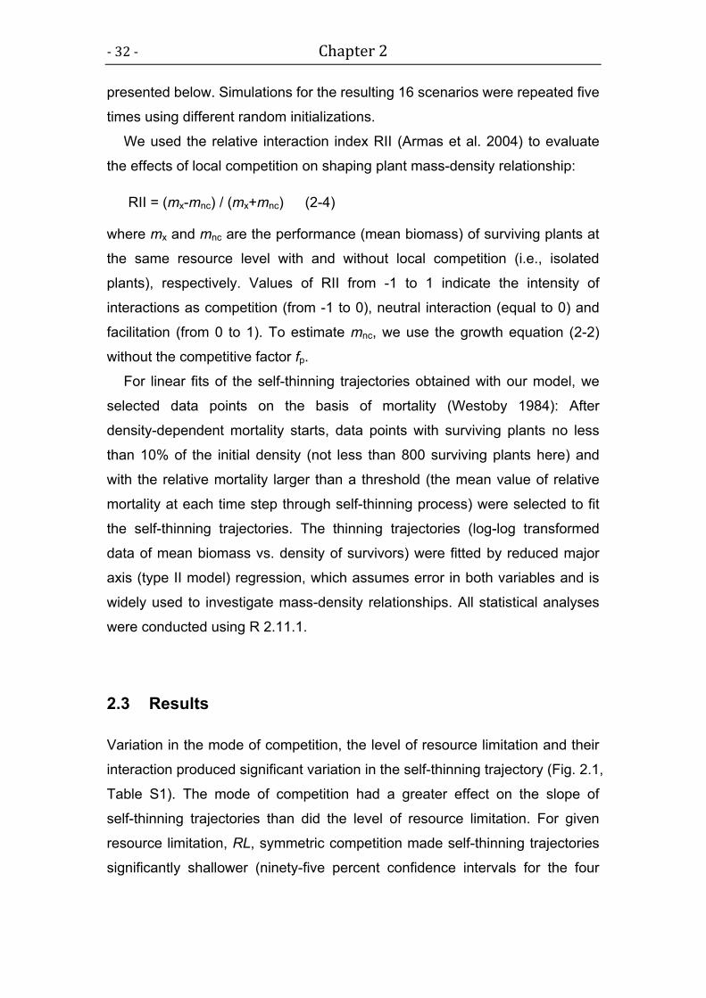
- 32 - Chapter 2

presented below. Simulations for the resulting 16 scenarios were repeated five

times using different random initializations.

We used the relative interaction index RII (Armas et al. 2004) to evaluate

the effects of local competition on shaping plant mass-density relationship:

RII = (mx-mnc) / (mx+mnc) (2-4)

where mx and mnc are the performance (mean biomass) of surviving plants at

the same resource level with and without local competition (i.e., isolated

plants), respectively. Values of RII from -1 to 1 indicate the intensity of

interactions as competition (from -1 to 0), neutral interaction (equal to 0) and

facilitation (from 0 to 1). To estimate mnc, we use the growth equation (2-2)

without the competitive factor fp.

For linear fits of the self-thinning trajectories obtained with our model, we

selected data points on the basis of mortality (Westoby 1984): After

density-dependent mortality starts, data points with surviving plants no less

than 10% of the initial density (not less than 800 surviving plants here) and

with the relative mortality larger than a threshold (the mean value of relative

mortality at each time step through self-thinning process) were selected to fit

the self-thinning trajectories. The thinning trajectories (log-log transformed

data of mean biomass vs. density of survivors) were fitted by reduced major

axis (type II model) regression, which assumes error in both variables and is

widely used to investigate mass-density relationships. All statistical analyses

were conducted using R 2.11.1.

2.3 Results

Variation in the mode of competition, the level of resource limitation and their

interaction produced significant variation in the self-thinning trajectory (Fig. 2.1,

Table S1). The mode of competition had a greater effect on the slope of

self-thinning trajectories than did the level of resource limitation. For given

resource limitation, RL, symmetric competition made self-thinning trajectories

significantly shallower (ninety-five percent confidence intervals for the four

Chapter 2 - 33 -

modes of competition did not overlap), but within same mode of competition

the level of resource limitation did not change slopes much (Fig. 2.2).

In scenarios with more symmetric competition, the relative interaction index

RII is close to -1 and thus the effect of competition on surviving individuals is

quite strong (Fig. 2.3). In contrast, in scenarios with more asymmetric

competition, surviving plants are less affected by interactions with other plants

(RII close to 0). The growth curves of plants also showed same results (Fig.

2.4). Both resource limitation and asymmetric competition lowered the position

of self-thinning trajectories: less biomass can be accumulated at a given

density under resource limitation or with more asymmetric competition (Fig.

2.1). Resource limitation decreased intercepts within the same mode of

competition (Fig. 2.2), which means that the maximum biomass of plants is

smaller in harsh conditions.

Fig. 2.1 Self-thinning trajectories for different levels of resource limitation and modes

of competition. RL indicates the level of resource limitation (from 0 to 1 indicating no

limitation to extreme limitation), p indicates the modes of competition (∞: completely

asymmetric; 10: highly size-asymmetric; 1: perfectly size-symmetric; 0: completely

symmetric). For comparison, the solid lines in figures have same intercepts and with

slopes equal to-4/3.

- 34 - Chapter 2

Fig. 2.2 Slopes and intercepts of self-thinning trajectories of mean individual biomass

versus survivor density under different levels of resource limitation and modes of

competition. RL indicates the level of resource limitation (from 0 to 1 indicating no

limitation to extreme limitation), p indicates the modes of competition (∞: completely

asymmetric; 10: highly size-asymmetric; 1: perfectly size-symmetric; 0: completely

symmetric). Bars indicate 95% confidence intervals.

Chapter 2 - 35 -

Fig. 2.3 Relationship between relative interaction intensity (RII) and density of

surviving plants at different levels of resource limitation and modes of competition. RL

indicates the level of resource limitation (from 0 to 1 indicating no limitation to extreme

limitation), p indicates the modes of competition (0: completely symmetric; 1: perfectly

size-symmetric; 10: highly size-asymmetric; ∞: completely asymmetric). Values of RII

indicate the intensity of interactions as competition (from -1 to 0), neutral interaction

(equal to 0) and facilitation (from 0 to 1).

- 36 - Chapter 2

Fig. 2.4 Growth curves of surviving plants at different levels of resource limitation and

modes of competition. RL indicates the level of resource limitation (from 0 to 1

indicating no limitation to extreme limitation), p indicates the modes of competition (0:

completely symmetric; 1: perfectly size-symmetric; 10: highly size-asymmetric; ∞:

completely asymmetric; NC: isolated growth without competition). Values of RII

indicate the intensity of interactions as competition (from -1 to 0), neutral interaction

(equal to 0) and facilitation (from 0 to 1).

Chapter 2 - 37 -

2.4 Discussion

Our results and those of previous studies (Stoll et al. 2002, Chu et al. 2010)

are consistent with our first hypothesis that symmetric competition can lead to

shallower self-thinning trajectories than asymmetric competition. This

suggests that deviations from the slope predicted by MST are likely to occur

when competition below ground is stronger than above ground because the

former is size-symmetric (Weiner et al. 1997, Schwinning and Weiner 1998).

Indeed, several empirical studies show that slopes of self-thinning trajectories

are significantly flatter under severe water stress (Deng et al. 2006) and low

nutrient levels (Morris 2003), conditions in which competition below ground is

thought to be more important than above ground (Schwinning and Weiner

1998, Deng et al. 2006, Berger et al. 2008). Furthermore, boreal coniferous

forests tend to have steeper slopes than deciduous broadleaved forests

because the canopy of conifers is denser (with lower light transmittance)

suggesting that asymmetric competition for light is more intense (Westoby

1984, Stoll et al. 2002, Li et al. 2006).

Why does symmetric competition lead to flatter trajectories in our model

even though it makes surviving plants larger on average at a given density (Fig.

2.1)? With symmetric competition, the growth of all individuals is significantly

reduced but the onset of mortality is delayed (Weiner et al. 2001 p. 20). Plants

can survive and grow even at relatively high densities, meaning that more

biomass can be maintained at a given density when competition is

size-symmetric (Stoll et al. 2002).

When competition is highly size asymmetric, surviving plants are less

affected by their neighbors and thus individual-level metabolic processes of

MST predict plant mass-density relationship at the population level: the slope

of the self-thinning trajectories are close to -4/3. This is consistent with our

second hypothesis that MST's predictions of population-level mass-density

relationships are successful when surviving plants are barely affected by local

interactions. In stands of Nothofagus solandri (mountain beech), taller trees

are relatively unhindered by competition for light and show the scaling of

diameter growth which is consist with prediction of MST, whereas small trees

affected by asymmetric competition do not follow the growth trajectory of

- 38 - Chapter 2

prediction (Coomes and Allen 2007, Coomes et al. 2011). In a tropical

rainforest, the trees under high-light conditions, i.e. being barely affected by

neighboring trees, their diameter growth was not significantly different from the

predictions of MST (Rüger and Condit 2012), which we also find in our model

(Fig. S1) and support our second hypothesis.

In contrast to our findings, Coomes and coworkers concluded that

deviations from predictions of MST in forests are caused by size-asymmetric

competition (Coomes and Allen 2007, Coomes et al. 2011). On closer

inspection, our results are not inconsistent with those of Coomes and

coworkers’. Coomes's studies focused on diameter growth of individuals,

including small suppressed individuals that are experiencing size-asymmetric

competition for light, whereas we focus here on the mass-density relationship

of populations during self-thinning, i.e. on plants surviving competition. When

competition is highly size-asymmetric, total biomass is primarily due to the

largest individuals, which are not highly affected by neighbors. If one looks,

however, at smaller individuals suffering from asymmetric competition before

they die, they will be highly affected by their larger neighbors, and this will be

more important for their growth and density than the internal relationships that

form the basis for MST. It would be worthwhile to analyze individual-level

diameter growth in our model to compare the patterns with those from

empirical studies (Coomes and Allen 2007, Coomes et al. 2011, Rüger and

Condit 2012) to see if the conclusions are consistent. Nevertheless, we agree

with Coomes and coworkers on the central point: interactions among

individuals can overrule the predictions of MST.

Both size-asymmetric competition and resource limitation lowered

self-thinning trajectories (Fig. 2.2). Resource limitation reduces the growth of

individual plants, leading to smaller individuals. Size-asymmetric competition

results in faster mortality. The reduction of biomass due to mortality is not

immediately compensated by the growth of survivors, so there is less total

biomass at a given density.

Using a similar model, Chu et al. (2010) found the same effect of the mode

of competition (size symmetric vs. asymmetric) on the slope of self-thinning

trajectories. The most important difference between Chu et al.'s model and

ours is that we used an individual growth model that is derived from MST,

Chapter 2 - 39 -

whereas they used the phenomenological growth equation of Weiner et al.

(2001). Chu et al. (2010) focused on the effects of mode of competition,

resource levels, and facilitation on self-thinning per se, so they do not refer to

MST or focus on their choice of their individual growth model. This may be why

the range of scaling exponent predicted with our model (-1.083 to -1.486) is

closer to the observed range of exponents (-1.103 to -1.441 for 1266 plots of

six biomes and 17 forest types across China) (Li et al. 2006) than models

using phenomenological growth functions (-0.8204 to -1.6095) (Chu et al.

2010). This suggests that the consideration of both neighborhood interactions

and constraints provided by MST are necessary to explain the

biomass-density relationships observed in the field.

Our results point to the scope and limits of MST at the population and

community level. MST applies to individual organisms, not always and

necessarily to populations or ecosystems. In some cases, for example where

resources are not limiting and competition is highly size-asymmetric, the

mass-density scaling exponent predicted by MST matches observations very

well. This is because individual acquisition of resources and accumulation of

biomass is driven primarily by what the individual itself does rather than by

interactions with other individuals (Fig. 2.3). On the other hand, when

individual behaviour is determined more by interactions with their neighbors

rather than processes that are the bases of MST, the population-level

behaviour will deviate from the predictions of MST.

Acknowledgements

We thank Sven Wagner, Angelika Körner, Christine Lemke, Cyril Piou, Antje

Karge, and Heinz Wolf for their kind help. James Brown and Jianming Deng

gave constructive comments on an earlier version of the manuscript. We also

thank two anonymous reviewers for their constructive comments on the

manuscript. The first author is supported by Helmholtz Impulse and

Networking Fund through Helmholtz Interdisciplinary Graduate School for

Environmental Research (HIGRADE).

http://tu-dresden.de/die_tu_dresden/fakultaeten/fakultaet_forst_geo_und_hydrowissenschaften/fachrichtung_forstwissenschaften/institute/wb/waldbau/dateien/wagner

- 40 - Chapter 2

References

Allen, A. P., W. T. Pockman, C. Restrepo, and B. T. Milne. 2008. Allometry, growth and

population regulation of the desert shrub Larrea tridentata. Functional Ecology

22:197–204.

Armas, C., R. Ordiales, and F. I. Pugnaire. 2004. Measuring plant interactions: a new

comparative index. Ecology 85:2682–2686.




9:121–135.




and G. Wang. 2010. Effects of positive interactions, size symmetry of competition

and abiotic stress on self-thinning in simulated plant populations. Annals of

Botany.

Coomes, D. A., and R. B. Allen. 2007. Effects of size, competition and altitude on tree

growth. Journal of Ecology 95:1084–1097.




Dai, X., X. Jia, W. Zhang, Y. Bai, J. Zhang, Y. Wang, and G. Wang. 2009. Plant

height–crown radius and canopy coverage–density relationships determine

above-ground biomass–density relationship in stressful environments. Biology

Letters 5:571–573. doi: 10.1098/rsbl.2009.0228.

Deng, J. M., G. E. N. . Wang, E. C. Morris, X. P. Wei, D. X. I. . Li, B. A. O. . Chen, C. M.

Zhao, J. Liu, and Y. Wang. 2006. Plant mass–density relationship along a

moisture gradient in north‐west China. Journal of Ecology 94:953–958.


general quantitative theory linking plant form and function from cells to

ecosystems. Tree Physiology 22:1045.

Enquist, B. J., J. H. Brown, and G. B. West. 1998. Allometric scaling of plant energetics

and population density. Nature 395:163–165.

Enquist, B. J., and K. J. Niklas. 2001. Invariant scaling relations across tree-dominated

communities. Nature 410:655–660.

Enquist, B. J., G. B. West, and J. H. Brown. 2009. Extensions and evaluations of a

general quantitative theory of forest structure and dynamics. Proceedings of the

National Academy of Sciences 106:7046.

Grimm, V., U. Berger, F. Bastiansen, S. Eliassen, V. Ginot, J. Giske, J. Goss-Custard, T.

Grand, S. K. Heinz, and G. Huse. 2006. A standard protocol for describing

individual-based and agent-based models. Ecological Modelling 198:115–126.

Grimm, V., U. Berger, D. L. DeAngelis, J. G. Polhill, J. Giske, and S. F. Railsback. 2010.

The ODD protocol: a review and first update. Ecological Modelling.

Hou, C., W. Zuo, M. E. Moses, W. H. Woodruff, J. H. Brown, and G. B. West. 2008.

Energy uptake and allocation during ontogeny. science 322:736.

Lambers, H., Chapin, F.S. & Pons, T.L. (2008). Plant physiological ecology. Springer

Verlag. pp. 134-143

Chapter 2 - 41 -

Li, H. T., X. G. Han, and J. G. Wu. 2006. Variant scaling relationship for mass-density

across tree-dominated communities. Journal of Integrative Plant Biology

48:268–277.

Lin, Y., U. Berger, V. Grimm, and Q.-R. Ji. 2012. Differences between symmetric and

asymmetric facilitation matter: exploring the interplay between modes of positive

and negative plant interactions. Journal of Ecology 100:1482–1491.

Morris, E. C. 2003. How does fertility of the substrate affect intraspecific competition?

Evidence and synthesis from self-thinning. Ecological Research 18:287–305.

Rüger, N., and R. Condit. 2012. Testing metabolic theory with models of tree growth that

include light competition. Functional Ecology 26:759–765.

Schwinning, S., and J. Weiner. 1998. Mechanisms determining the degree of size

asymmetry in competition among plants. Oecologia 113:447–455.


competition alters biomass–density relationships. Proceedings of the Royal

Society of London. Series B: Biological Sciences 269:2191.

Weiner, J., P. Stoll, H. Muller-Landau, and A. Jasentuliyana. 2001. The effects of density,

spatial pattern, and competitive symmetry on size variation in simulated plant

populations. The American Naturalist 158:438–450.

Weiner, J., and S. C. Thomas. 1992. Competition and allometry in three species of annual

plants. Ecology 21:648–656.

Weiner, J., D. B. Wright, and S. Castro. 1997. Symmetry of below-ground competition

between Kochia scoparia individuals. Oikos 79:85–91.

West, G. B., J. H. Brown, and B. J. Enquist. 1999. The fourth dimension of life: fractal

geometry and allometric scaling of organisms. Science 284:1677.

West, G. B., J. H. Brown, and B. J. Enquist. 2001. A general model for ontogenetic growth.

Nature 413:628–631.

Westoby, M. 1984. The self-thinning rule. Advances in ecological research 14:167–226.

Wilensky, U. 1999. Netlogo. http://ccl.northwestern. edu/netlogo/. Center for Connected

Learning and Computer-Based Modeling, Northwestern University, Evanston, IL.

Zhang, W.P., X. Jia, Y.Y. Bai, and G.X. Wang. 2011. The difference between above- and

below-ground self-thinning lines in forest communities. Ecological Research

26:819–825.

- 42 - Chapter 2

Chapter 2 – Appendix A

A general ontogenetic growth model for plants

The essential basis for modelling the ontogeny of individual plants starts with

an energy conservation equation (Enquist and Niklas 2001; West et al. 2001;

Hou et al. 2008):

Bp = Br + Bs = Br + Esdm/dt (2-A1)

where Bp is defined as total energy intake rate (i.e. gross photosynthetic rate).

A fraction of this assimilated energy is consumed by respiration, Br, the

remainder is stored as reserves and Bs is used for synthesizing new tissues

(and for reproducing) (Figure A1). Es is the metabolic energy stored in one unit

of biomass and dm/dt is the change in biomass (m) per unit time (t).

Figure A1 Assimilated energy partition of plants during ontogenetic growth.

The rate of energy consumed by respiration, Br, depends on three major

processes that require energy (Figure A1): maintenance of biomass (Bmaint),

ion transport (Btran) and biosynthesis (Bsyn), which can be summarized as

(Lambers et al. 2008):

Br = Bmaint + Btran + Bsyn = ∑Bmmliving + Btran + Ecdm/dt (2-A2)

Whole-plant photosynthetic

rate (Bp)

Energy consumed by

respiration (Br)

Rate of energy for maintenance

(Bmaint)

Rate of energy for photosynthetic

tissue (BL=BmmL)

Rate of energy for conducting tissue

(BC=BmmC)

Rate of energy for ion transport

(Btran)

Rate of energy for biosyntheses (Bsyn=Emdm/dt)

Rate of energy stored

(Bs=Esdm/dt)

Chapter 2 - 43 -

where Bm denotes average mass-specific maintenance metabolic rate, mliving

stands for the biomass of living tissues, and Ec designates the energy required

to synthesize a unit of biomass.

Typical average biological parameters of plant cells (tissue) are taken as a

fundamental unit here, and possible differences between tissues are ignored

(West et al. 2001). Note that the terms Bs=Esdm/dt in Eqn (2-A1) and

Bsyn=Ecdm/dt in Eqn (2-A2) are quite different: S stands for the rate of

cumulative energy content of new biomass, whereas Bsyn refers to the

metabolic energy expended on biosynthesis which is dissipated as heat

instead of obtained as stored biomass (Hou et al. 2008). Combining Eqns

(2-A1) and (2-A2), we get

Bp = Bmaint + Btran + Bsyn + Bs = ∑Bmmliving + Btran + E0dm/dt (2-A3)

where E0 = Ec+Es, is constant for a given taxon and stands for the sum of

energy stored in a unit of biomass plus the energy used to synthesize this

biomass, i.e. the synthesis costs of a unit of biomass.

Equation (2-A3) is quite general, but Bmaint may vary between woody and

non-woody plants, as woody plants contain nonliving tissues (e.g. heartwood

in stem and root) which do not need energy for their maintenance (Enquist et

al. 2009). Also large trees with a large amount of heartwood, contain much

less living tissues (mliving) in comparison to the total biomass (m). We assume

that during ontogeny, woody plants mainly expend energy for maintaining their

photosynthetic tissues (leaves), mL, and conducting tissues (standing

sapwood of stem and root), mC, and suppose

Bmaint = ∑Bmmliving = BmmL + BmmC = BL + BC (2-A4)

for woody plants, where BL and BC specify the metabolic rate for maintaining

photosynthetic and conducting tissues, respectively (Figure A1). Combining

Eqns (2-A3) and (2-A4) we can get the energy conservation equation for

woody plants:

Bp = BmmL + BmmC + Btran + E0 dm/dt (2-A5)

Based on empirical measurements and theoretical assumptions linking

biomass and metabolism, MST (West et al. 1999; Enquist 2002; Price et al.

2007; Enquist et al. 2009; West et al. 2009) predicts that whole-plant, or gross,

photosynthesis rate, Bp, and ion transport metabolic rate Btran allometrically

scale with the total biomass of a plant, m, as BpBtranmθ, where θ ≡ 1/(2α+β)

and α and β representing the geometry and biomechanics of the vascular

network. Their values may vary across different taxa (Price et al. 2007).

Although the Eqn (2-A5) can be easily recast by using empirical values of

α and β, we use α = 1/2 and β = 1/3 as common and idealized cases here

(Price et al. 2007; West et al. 2009), so that θ = 3/4. Models based on these

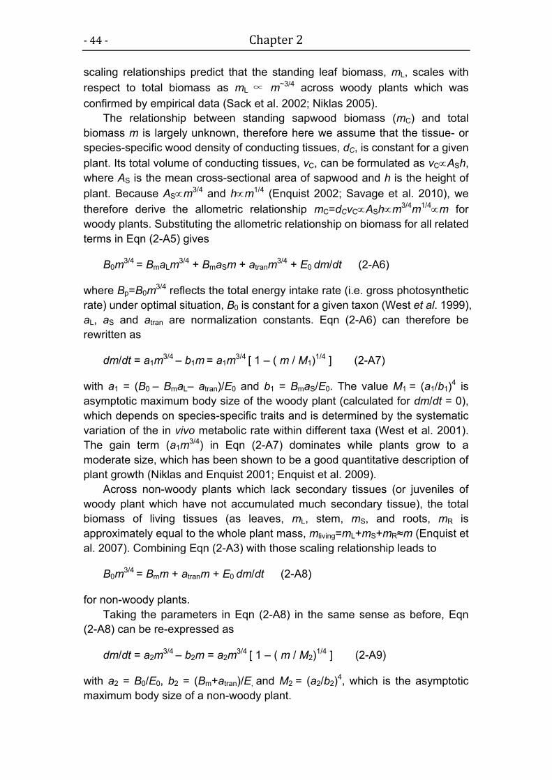
- 44 - Chapter 2

scaling relationships predict that the standing leaf biomass, mL, scales with

respect to total biomass as mL ∝ m~3/4 across woody plants which was

confirmed by empirical data (Sack et al. 2002; Niklas 2005).

The relationship between standing sapwood biomass (mC) and total

biomass m is largely unknown, therefore here we assume that the tissue- or

species-specific wood density of conducting tissues, dC, is constant for a given

plant. Its total volume of conducting tissues, vC, can be formulated as vCASh,

where AS is the mean cross-sectional area of sapwood and h is the height of

plant. Because ASm3/4 and hm1/4 (Enquist 2002; Savage et al. 2010), we

therefore derive the allometric relationship mC=dCvCAShm3/4m1/4m for

woody plants. Substituting the allometric relationship on biomass for all related

terms in Eqn (2-A5) gives

B0m3/4 = BmaLm

3/4 + BmaSm + atranm3/4 + E0 dm/dt (2-A6)

where Bp=B0m3/4 reflects the total energy intake rate (i.e. gross photosynthetic

rate) under optimal situation, B0 is constant for a given taxon (West et al. 1999),

aL, aS and atran are normalization constants. Eqn (2-A6) can therefore be

rewritten as

dm/dt = a1m3/4 – b1m

= a1m3/4 [ 1 – ( m / M1)

1/4 ] (2-A7)

with a1 = (B0 – BmaL– atran)/E0 and b1 = BmaS/E0. The value M1 = (a1/b1)4 is

asymptotic maximum body size of the woody plant (calculated for dm/dt = 0),

which depends on species-specific traits and is determined by the systematic

variation of the in vivo metabolic rate within different taxa (West et al. 2001).

The gain term (a1m3/4) in Eqn (2-A7) dominates while plants grow to a

moderate size, which has been shown to be a good quantitative description of

plant growth (Niklas and Enquist 2001; Enquist et al. 2009).

Across non-woody plants which lack secondary tissues (or juveniles of

woody plant which have not accumulated much secondary tissue), the total

biomass of living tissues (as leaves, mL, stem, mS, and roots, mR is

approximately equal to the whole plant mass, mliving=mL+mS+mR≈m (Enquist et

al. 2007). Combining Eqn (2-A3) with those scaling relationship leads to

B0m3/4 = Bmm + atranm + E0 dm/dt (2-A8)

for non-woody plants.

Taking the parameters in Eqn (2-A8) in the same sense as before, Eqn

(2-A8) can be re-expressed as

dm/dt = a2m3/4 – b2m = a2m

3/4 [ 1 – ( m / M2)1/4 ] (2-A9)

with a2 = B0/E0, b2 = (Bm+atran)/E, and M2 = (a2/b2)4, which is the asymptotic

maximum body size of a non-woody plant.

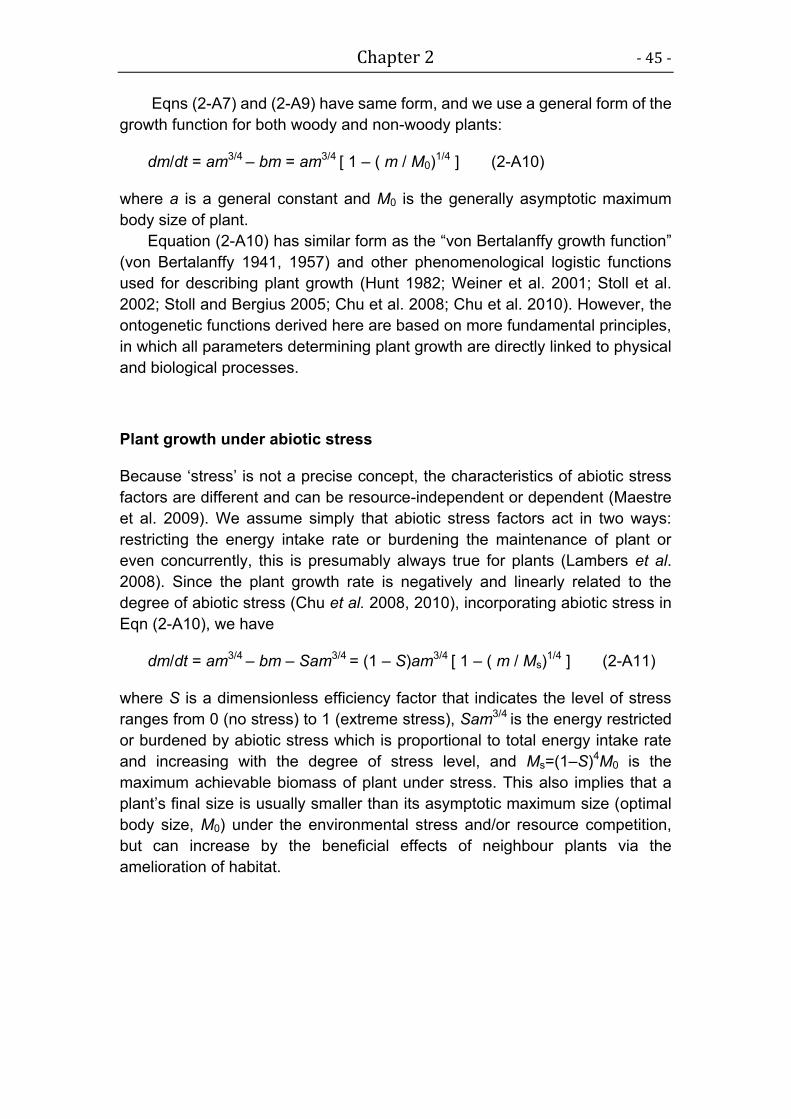
Chapter 2 - 45 -

Eqns (2-A7) and (2-A9) have same form, and we use a general form of the

growth function for both woody and non-woody plants:

dm/dt = am3/4 – bm = am3/4 [ 1 – ( m / M0)1/4 ] (2-A10)

where a is a general constant and M0 is the generally asymptotic maximum

body size of plant.

Equation (2-A10) has similar form as the “von Bertalanffy growth function”

(von Bertalanffy 1941, 1957) and other phenomenological logistic functions

used for describing plant growth (Hunt 1982; Weiner et al. 2001; Stoll et al.

2002; Stoll and Bergius 2005; Chu et al. 2008; Chu et al. 2010). However, the

ontogenetic functions derived here are based on more fundamental principles,

in which all parameters determining plant growth are directly linked to physical

and biological processes.

Plant growth under abiotic stress

Because ‘stress’ is not a precise concept, the characteristics of abiotic stress

factors are different and can be resource-independent or dependent (Maestre

et al. 2009). We assume simply that abiotic stress factors act in two ways:

restricting the energy intake rate or burdening the maintenance of plant or

even concurrently, this is presumably always true for plants (Lambers et al.

2008). Since the plant growth rate is negatively and linearly related to the

degree of abiotic stress (Chu et al. 2008, 2010), incorporating abiotic stress in

Eqn (2-A10), we have

dm/dt = am3/4 – bm – Sam3/4 = (1 – S)am3/4 [ 1 – ( m / Ms)1/4 ] (2-A11)

where S is a dimensionless efficiency factor that indicates the level of stress

ranges from 0 (no stress) to 1 (extreme stress), Sam3/4 is the energy restricted

or burdened by abiotic stress which is proportional to total energy intake rate

and increasing with the degree of stress level, and Ms=(1–S)4M0 is the

maximum achievable biomass of plant under stress. This also implies that a

plant’s final size is usually smaller than its asymptotic maximum size (optimal

body size, M0) under the environmental stress and/or resource competition,

but can increase by the beneficial effects of neighbour plants via the

amelioration of habitat.

- 46 - Chapter 2

Extensions and predictions based on the general growth model of plant

A general stem diameter growth model of plants

Sometimes, to get the whole biomass of plants is difficulty, especially when we

are going to measure trees. It is therefore flexible to use stem diameter (D)

instead of biomass (m). Since D∝m3/8, which is equivalent to f(D)=dD/dm∝

m-5/8, then dD/dt=f(D)(dm/dt) combine with Eqs. (2-A7), (2-A9) and (2-A10), we

have

dD/dt = adD1/3 – bdD

4/3 = adD1/3 [ 1 – (D / Dmax) ] (2-A12)

where ad and bd are constants, Dmax =ad /bd is the asymptotic maximum stem

diameter.

The sigmoid growth curve of plants

A general sigmoid growth model for plants can be obtained from integrating

Equation (2-A10):

1/4

1/4

1/4 1/4

/40

0 0

4

1/4 /40

0

1 1

or 1 [1 ( ) ]

at M

at M

mme

M M

mam e

b M

(2-A13)

where m0 is the initial biomass of the plant (biomass at birth, t=0).

In the expression related to stem diameter,

1/3d max

1/3 1/3

/30

max max

1 1

a t DDDe

D D (2-A14)

where D0 is the initial diameter of the plant (t=0).

Currently, we are not able to combine the data sets that are precise

enough and also cover a broad plant species to test our model. However,

based on a recent publishes work (Deng et al. 2012), we tested our model with

three non-woody plants, the mechanistic model are proved to be reliable

(Figure A2). How well of our model in capturing the fundamental features of

growth in woody and non-woody plants are remains to be seen.

Chapter 2 - 47 -

Figure A2 Growth curves for wheat, flax, and Arabidopsis. The curves are the

predictions of the general growth model (Equation. 2-E2). Growth data are estimated

from Deng et al. (2012).

A general model for respiratory metabolism of plant

Overall, the respiratory metabolism of plant can be generally summarized in

equation (2-A2). For woody plant, because of the growth rate dm/dt ≈ acm3/4,

where ac is a constant, hence the respiration rate of woody plants is:

Br = BmaLm3/4 + BmaSm + atranm

3/4 + Ec dm/dt = arm3/4 + brm (2-A15)

where ar= BmaL+atran+ Ecac and br=BmaS.

Equation (2-A15) indicates a mixed scaling relationship of rate of energy

consumed by respiration for woody and non-woody plants, i.e. the theoretical

scaling exponent between whole respiration rate of plant and its whole

biomass, Br vs. m, can range from 0.75 to 1 which depends on the values of ar

and br, and is related to the productive biomass partitioning among different

compartments (e.g. leaf, branch, stem, root, and seed reproduction). However,

for woody plants with much of secondary tissues, the scaling should approach

0.75, but for non-woody plants or juveniles of woody plant which haven’t

accumulated much of secondary tissues, the scaling exponent between

respiratory metabolism and biomass will approach to 1. These variations were

perceived in empirical researches (Reich et al. 2006; Enquist et al. 2007;Mori

et al. 2010; Cheng et al. 2010).

- 48 - Chapter 2

Scaling relationship between reproductive biomass and mean body mass of

seed plants

Based on MST and equation (2-A10), the plant reproductive biomass should

proportional to its metabolic rate, and then we predict a simple scaling

relationship between reproductive biomass (mrep.) and plant body mass (m) as

mrep. m 3/4 (2-A16)

using a broad data set (Niklas and Enquist 2004) of seed plants, we proved the

validity of this prediction (Figure A3).

Figure A3 The scaling relationship between mean plant mass (m) and mean

reproduction mass (mrep.) across different species of of seed plants. The solid line

shows the fitted Reduced Major Axis (RMA, type II model) regression of equation (95%

C.I. of the exponent 0.70–0.77).

Chapter 2 - 49 -

ODD protocol – model description of one-layer pi model

The following model description follows the ODD protocol (Overview, Design


et al. 2006; Grimm et al. 2010),

Purpose

The aim of this model is to evaluate the multiple effects of the mode of

competition and resource limitation on regulating plant population dynamics,

specifically on self-thinning trajectories and density-dependent mortality. In

particular, we investigate whether interactions on individual plant level can

alter the slope and intercept of the self-thinning line. The model does not

represent specific species, but generic ones.

Entities, state variables, and scales

The entities in the model are plants and square habitat units, or patches (Table

A1). Plants are characterized by the following state variables: initial growth

rate, initial biomass, maximum biomass (asymptotic biomass), current

biomass and their position, i.e. coordinates of the stem. Each individual plant

has its own circular zone-of-influence (ZOI). The ZOI stands for the physical

space occupied by a plant, and represents the energy and resources

potentially available to this plant, which is allometrically related to its body

mass. Neighboring plants only compete for the resources when their ZOIs are

overlapping.

In order to make the spatial calculations of resource competition easier,

ZOIs are projected onto a grid of patches. To avoid edge effects, we use a

torus world with a size of 200 × 200 patches (Grimm & Railsback 2005). Each

patch represents 0.25 m2 or 0.25 cm2 for woody- and non-woody plants,

respectively. The state of each patch is characterized by its resource

availability. We use a homogeneous environment here as all patches have the

same, and constant, degree of resource limitation. One time step in the model

represents approximately one year for woody plants and one day for

non-woody plants.

- 50 - Chapter 2

Table A1. State variables and initialization in the individual-based model. Actual

values are drawn from the given intervals to introduce a certain degree of

heterogeneity among individuals.

Variable Description Initial Value [unit]

(woody/non-woody)

Plants

c Initial growth rate 1 ± 0.1 [kg m-2 time step-1] /

[mg cm-2 time step-1]

m0 Initial body mass 2 ± 0.2 [kg] / [mg]

M Maximal biomass 2×106 ± 2×105 [kg] / [mg]

m Current biomass [kg] / [mg]

A Zone of influence [m-2] / [cm-2]

Patches

RL Level of resource limitation [0, 1]

Initialization

Mortality Threshold of death 2% of m3/4

Density Number of plants 8100 ha-1 / m-2

Process overview and scheduling

After initialization, all individual plants with a given density are randomly

distributed in the world. The processes of resource competition, growth and

mortality of each plant are fulfilled within each time step. In each step,

individual plants first sense the resource qualities of patches within their ZOIs,

the area (radius) of an individual plant’s ZOI is determined by its current

biomass. When their ZOIs are overlapping, individuals compete within the

overlapping area. Thus, the overlapping area reflecting resources is divided

according to the competition mode. Considering the outcome of the

competition process, all individual plants grow according to the growth function.

Plants with growth rates falling below a threshold die and are removed

immediately. The state variables of the plants are synchronously updated

within the subroutines, i.e. changes to state variables are updated only after all

individuals have been processed (Grimm and Railsback 2005).

Design concepts

Basic principles: From “Metabolic Scaling Theory”, we derived a general

ontogenetic growth model for individual plants. We combine this model, via the

ZOI approach, with the effects of different modes of competition and resource

limitation.

Emergence: All features observed at the population level, e.g. mass-density

relationship or self-thinning trajectories (i.e. size distribution and spatial

distribution, respectively), emerge from the interaction of individual plants with

their neighbors and the resource level of their abiotic environment.

Chapter 2 - 51 -

Interaction: Individual plants interact via competition for resources in the

overlapping area of their ZOIs.

Stochasticity: Initial growth rate, initial biomass, maximum biomass and initial

position of plants are randomly taken from the intervals given in Table 1. This

introduces a certain level of heterogeneity among individual characteristics to

take into account that real plants are never exactly identical.

Observation: Population size, biomass of each plant, and mean biomass of all

living plants are the main observations.

Initialization

Initially, individual plants are randomly distributed according to the chosen

initial density. Resources are spatially and temporally constant. Each plant has

an initial biomass (m0), maximal biomass (M) and initial growth rate (c1 or c2)

drawn from truncated normal distributions with average and intervals given in

Table 1.

Input

After initialization, the model does not include any external inputs, i.e. the

abiotic environment is constant.

Submodels

Plant growth

In our individual-based model the plant’s ZOI stands for the physical space

occupied by a plant and represents the energy and resources potentially

available to this plant. This space is allometrically related to the plant’s body

mass, m, as c0A=m3/4 (Enquist & Niklas 2001), where c0 is a normalization

constant. Accordingly, based on equation (2-A1) we have:

dm/dt = cA[ 1 – ( m / M0 )1/4 ] (2-M1)

where c = ac0 is initial growth rates in units of mass per area and time interval.

For simplicity, we choose 1 ± 0.1 in our model. We also simulate the model

with different c values. As expected, the results from different values were

qualitatively similar (the slopes didn’t change).

Resource competition and limitation

Resource limitation and competition usually cause a reduction of resource

availability for plants. We therefore represent resource limitation via a

dimensionless efficiency factor or index, fR, for different levels of resource

availability. Resource competition is incorporated by using a dimensionless

competition factor or index, fp, leading to

dm/dt = fRfpcA[ 1 – ( m / M )1/4 ] (2-M2)

- 52 - Chapter 2

where M = (fRfp)4M0, the maximum body size with resource limitation and

competition.

The efficiency factor fR, can take different forms depending on the

characteristics and level of the limiting resource. For simplification, we use a

linear form here, i.e. fR = 1–RL, where RL indicates the level of resource

limitation, with its value ranging from 0 (no resource limitation) to 1 (maximum

resource limitation; Table A1).

As for competition, the mode of resource-mediated competition among

plants can be located somewhere along a continuum between completely

asymmetric competition (largest plants obtain all the contested resources) and

completely symmetric competition (resource uptake is equal for all plants,

independent of their relative sizes; Schwinning & Weiner 1998). To represent

different modes of competition explicitly, we describe the competitive factor fp

as

,1

1

( ) /

o

j

pn i

p no o k nk p

jj

mf A A A

m (2-M3)

This factor thus refers to the percentage of realized resource plant i could

uptake from the amount of resources available (the entire resource that plant

could potentially occupy) among nj competitors with sizes mj (Schwinning &

Weiner 1998). Ano is the area not overlapping with neighbors, Ao,k denotes the

area overlapping with neighbors. Parameter p determines the mode of

competition, ranging from complete symmetry (p = 0) to complete asymmetry

(p approaching infinity; for details and examples see Figure A4).

Figure A4. An example of calculating the competitive index (equation 2-M3)

with different modes of resource competition in an individual-based model as a

Chapter 2 - 53 -

way of dividing plants’ ZOI (zone-of-influence). Three plants with sizes m1, m2

and m3 are competing in this example. For plant 1, its ZOI (A) was divided into

four parts: Ano, the area not overlapping with the other two plants; Ao,1, the area

overlapping with plant 2; Ao,2, the area overlapping with plants 2 and 3; Ao,3,

the area overlapping with plant 3.

Then the actual area that plant 1 can take from Ao,1 is

1 1,1 ,12

1 21

p p

o o p pp

jj

m mA A

m mm

For Ao,2,

1 1,2 ,23

1 2 31

p p

o o p p pp

jj

m mA A

m m mm

And for Ao,3,

1 1,3 ,32

1 31

p p

o o p pp

jj

m mA A

m mm

Therefore, the competitive index for plant 1 is:

Where 3/4

1 0/A m c

In total, equation (2-M2) clearly shows how a plant’s growth rate is jointly

determined by resource availability, fR, and competition, fp. This also implies

that a plant’s final size is usually smaller than its asymptotic maximum size (M)

during resource limitation and local competition.

Mortality

An individual’s mortality rate is proportional to its mass-specific metabolism

(Brown et al. 2004). Based on this, we assume that individuals die if their

actual growth rate (dm/dt) falls below a threshold of their current scaled body

mass, i.e. 2% of m3/4. Therefore, individual plants may die due to metabolic

inactivation driven by resource limitation, competition, senescence (when m

approaches M) or combinations thereof. This provides a more realistic

representation of relevant ecological process than in previous models (Stoll et

al. 2002; Chu et al. 2010).

- 54 - Chapter 2

References

von Bertalanffy, L. 1941. Stoffwechseltypen und Wachstumstypen. Untersuchungen über

die Gesetzlichkeit des Wachstums VII, Biologisches Zentralblatt, 61, 511–532.

von Bertalanffy, L. 1957. Quantitative laws in metabolism and growth. Quarterly Review of

Biology 32:217–231.

Brown, J.H., Gillooly, J.F., Allen, A.P., Savage, V.M. & West, G.B. (2004). Toward a

metabolic theory of ecology. Ecology, 85, 1771–1789.

Cheng, D.L., T. Li, Q.L. Zhong, and G.X. Wang. 2010. Scaling relationship between tree respiration rates and biomass. Biology Letters 6:715 –717.

Chu, C. J., F. T. Maestre, S. Xiao, J. Weiner, Y. S. Wang, Z. H. Duan, and G. Wang. 2008. Balance between facilitation and resource competition determines biomass–density relationships in plant populations. Ecology Letters 11:1189–1197.

Chu, C.J., Weiner, J., Maestre, F.T., Wang, Y.S., Morris, C., Xiao, S., et al. (2010). Effects

of positive interactions, size symmetry of competition and abiotic stress on

self-thinning in simulated plant populations. Annals of Botany, 106, 647–652.

Deng, J., J. Ran, Z. Wang, Z. Fan, G. Wang, M. Ji, J. Liu, Y. Wang, J. Liu, and J. H. Brown. 2012. Models and tests of optimal density and maximal yield for crop plants. Proceedings of the National Academy of Sciences 109:15823–15828.

Enquist, B. J. 2002. Universal scaling in tree and vascular plant allometry: toward a general quantitative theory linking plant form and function from cells to ecosystems. Tree Physiology 22:1045.

Enquist, B. J., A. P. Allen, J. H. Brown, J. F. Gillooly, A. J. Kerkhoff, K. J. Niklas, C. A. Price, and G. B. West. 2007. Biological scaling: Does the exception prove the rule? Nature 445:E9–E10.

Enquist, B.J. & Niklas, K.J. (2001). Invariant scaling relations across tree-dominated

communities. Nature, 410, 655–660.

Enquist, B. J., G. B. West, and J. H. Brown. 2009. Extensions and evaluations of a general quantitative theory of forest structure and dynamics. Proceedings of the National Academy of Sciences 106:7046–7052.

Grimm, V., Berger, U., Bastiansen, F., Eliassen, S., Ginot, V., Giske, J., et al. (2006). A

standard protocol for describing individual-based and agent-based models.

Ecological Modelling, 198, 115–126.

Grimm, V., Berger, U., DeAngelis, D.L., Polhill, J.G., Giske, J. & Railsback, S.F. (2010).

The ODD protocol: A review and first update. Ecological Modelling, 211,

2760–2768.

Grimm, V. & Railsback, S.F. (2005). Individual-based modeling and ecology. Princeton

University Press.

Hou, C., W. Zuo, M. E. Moses, W. H. Woodruff, J. H. Brown, and G. B. West. 2008. Energy uptake and allocation during ontogeny. Science 322:736.

Hunt, R. 1982. Plant growth curves: the functional approach to plant growth analysis. Arnold.

Lambers, H., F. S. Chapin, and T. L. Pons. 2008. Plant physiological ecology. Springer Verlag.

Maestre, F. T., R. M. Callaway, F. Valladares, and C. J. Lortie. 2009. Refining the stress-gradient hypothesis for competition and facilitation in plant communities. Journal of Ecology 97:199–205.

Mori, S., K. Yamaji, A. Ishida, S. G. Prokushkin, O. V. Masyagina, A. Hagihara, A. T. M. R. Hoque, R. Suwa, A. Osawa, T. Nishizono, T. Ueda, M. Kinjo, T. Miyagi, T. Kajimoto, T. Koike, Y. Matsuura, T. Toma, O. A. Zyryanova, A. P. Abaimov, Y. Awaya, M. G. Araki, T. Kawasaki, Y. Chiba, and M. Umari. 2010. Mixed-power scaling of whole-plant respiration from seedlings to giant trees. Proceedings of the National Academy of Sciences of the United States of America 107:1447-1451

Chapter 2 - 55 -

Niklas, K. J. 2005. Modelling below-and above-ground biomass for non-woody and woody plants. Annals of Botany 95:315.

Niklas, K. J., and B. J. Enquist. 2001. Invariant scaling relationships for interspecific plant biomass production rates and body size. Proceedings of the National Academy of Sciences of the United States of America 98:2922.

Price, C. A., B. J. Enquist, and V. M. Savage. 2007. A general model for allometric covariation in botanical form and function. Proceedings of the National Academy of Sciences 104:13204.

Reich, P. B., M. G. Tjoelker, J.-L. Machado, and J. Oleksyn. 2006. Universal scaling of respiratory metabolism, size and nitrogen in plants. Nature 439:457–461.

Sack, L., T. Maranon, P. J. Grubb, B. J. Enquist, and K. J. Niklas. 2002. Global allocation rules for patterns of biomass partitioning. Science 296:1923.

Savage, V. M., L. P. Bentley, B. J. Enquist, J. S. Sperry, D. D. Smith, P. B. Reich, and E. I. von Allmen. 2010. Hydraulic trade-offs and space filling enable better predictions of vascular structure and function in plants. Proceedings of the National Academy of Sciences 107:22722.

Schwinning, S. & Weiner, J. (1998). Mechanisms determining the degree of size

asymmetry in competition among plants. Oecologia, 113, 447–455.

Stoll, P. & Bergius, E. (2005). Pattern and process: competition causes regular spacing of

individuals within plant populations. Journal of Ecology, 93, 395–403.

Stoll, P., J. Weiner, H. Muller-Landau, E. Müller, and T. Hara. 2002. Size symmetry of competition alters biomass–density relationships. Proceedings of the Royal Society of London. Series B: Biological Sciences 269:2191.

Weiner, J., P. Stoll, H. Muller-Landau, and A. Jasentuliyana. 2001. The effects of density, spatial pattern, and competitive symmetry on size variation in simulated plant populations. American Naturalist 158:438–450.

West, G. B., J. H. Brown, and B. J. Enquist. 2001. A general model for ontogenetic growth. Nature 413:628–631.

West, G. B., B. J. Enquist, and J. H. Brown. 2009. A general quantitative theory of forest structure and dynamics. Proceedings of the National Academy of Sciences 106:7040–7045.

- 56 - Chapter 2

Slopes and intercepts of self-thinning trajectories produced by the model

Table S1. Slope and intercept (log-log transformed) of self-thinning trajectories for

simulated plants under different levels of resource limitation and modes of

competition*.

RL p

Slope Intercept

R2 Mean 95% C.I. Mean 95% C.I.

0 ∞ -1.478 -1.525 -1.429 6.258 6.096 6.424 0.994

0 10 -1.342 -1.361 -1.322 5.848 5.808 5.898 0.999

0 1 -1.140 -1.156 -1.125 5.714 5.664 5.769 0.997

0 0 -1.083 -1.085 -1.082 6.208 6.204 6.212 0.999

0.1 ∞ -1.478 -1.526 -1.427 6.217 6.074 6.377 0.994

0.1 10 -1.354 -1.374 -1.333 5.848 5.778 5.918 0.998

0.1 1 -1.144 -1.158 -1.130 5.697 5.650 5.744 0.997

0.1 0 -1.094 -1.098 -1.091 6.185 6.180 6.190 0.999

0.5 ∞ -1.480 -1.516 -1.445 6.176 6.060 6.297 0.995

0.5 10 -1.385 -1.402 -1.365 5.805 5.736 5.875 0.997

0.5 1 -1.188 -1.198 -1.179 5.554 5.519 5.585 0.998

0.5 0 -1.124 -1.126 -1.122 5.978 5.972 5.984 0.999

0.9 ∞ -1.486 -1.499 -1.472 5.918 5.873 5.963 0.996

0.9 10 -1.395 -1.401 -1.389 5.637 5.619 5.657 0.999

0.9 1 -1.201 -1.209 -1.194 5.370 5.345 5.395 0.998

0.9 0 -1.130 -1.139 -1.122 5.474 5.446 5.502 0.997

*RL indicates the level of resource limitation (0–1), p indicates the modes of

competition (with 0: completely symmetric; 1: perfectly size-symmetric; 10: highly

size-asymmetric; ∞: completely asymmetric). C.I. is confidence intervals.

Chapter 3

Mechanisms mediating plant mass-density

relationships: the role of biomass allocation,

above- and belowground competition *

Abstract

Metabolic scaling theory (MST) predicts a ‘universal scaling law’ for plant

mass-density relationships, but empirical observations are more variable.

Possible explanations of this deviation include plasticity in biomass allocation

between the above- and belowground compartment and the mode of

competition, which can be asymmetric or symmetric. Although complex

interactions of these factors are reasonable, the majority of modelling and

empirical studies have been focusing on mono-factorial explanations so far.

We present a generic individual-based model, which allows exploring MST

predictions in realistic settings by representing plasticity of biomass allocation

and different modes of competition in the above- and belowground

compartment simultaneously. To evaluate the behaviour of the simulated

plants related to the allocation patterns and to validate model predictions

* A slightly revised version of this chapter has been submitted to Ecology (status: under

review) as Yue Lin1, 2

, Franka Huth3, Uta Berger

1, and Volker Grimm

2, 4: Belowground

competition and biomass allocation explain deviations from the plant mass-density

relationship predicted by metabolic scaling theory

1 Institute of Forest Growth and Computer Science, Dresden University of Technology, P.O.

1117, 01735 Tharandt, Germany; 2 Helmholtz Centre for Environmental Research – UFZ,

Department of Ecological Modelling, 04318 Leipzig, Germany; 3 Institute of Silviculture

and Forest Protection, Dresden University of Technology, 01735 Tharandt, Germany; 4

Institute for Biochemistry and Biology, University of Potsdam, Maulbeerallee 2, 14469

Potsdam, Germany

- 58 - Chapter 3

regarding the mass-density relationship, we conducted greenhouse

experiments with tree seedlings. The simulated model well captured empirical

patterns both at plant individual and population level. Without belowground

resource limitation, aboveground processes dominated and the slopes of

mass-density relationships followed the predictions of MST. In contrast,

resource limitation resulted to an increased allocation of biomass to

belowground parts of the plants. The subsequent dominance of symmetric

belowground competition led to significantly shallower slopes of the

mass-density relationship. We conclude that changes in biomass allocation

patterns control the constraints at different levels of biological organization and

explain the deviations from the mass-density relationship predicted by MST.

Taking into account the plasticity of biomass allocation and its linkage to the

visible aboveground competition and the invisible belowground competition is

critical for fully representing many forests and eco-regions, in particular for

correctly predicting the response of carbon storage and sequestration to

changing environmental conditions.

Keywords: plasticity, biomass allocation, optimization theory, symmetric

competition, asymmetric competition, ontogenetic growth of plant,

individual-based model, allometric exponent, power law

3.1 Introduction

The relationship between plant performance and density is one of the central

topics in plant ecology (Stoll et al. 2002, Deng et al. 2006, Chu et al. 2010,

Weiner and Freckleton 2010). It is widely accepted that resource competition

among plants is the main force in determining plant mass-density relationships

induced by density-dependent mortality. In self-thinning stands of plants, the

general relationship between density (N) and mean biomass (My) of surviving

plants can be described by a power function, My=kNγ, where k and γ are

referred to as the thinning coefficient and exponent, respectively. Based on

Euclidean geometry, it was proposed that the value of γ is approximately equal

to -3/2, which is well-known as the “-3/2 power rule” of self-thinning (Yoda et al.

Chapter 3 - 59 -

1963). More recently, based on a fractal model metabolic scaling theory (MST)

predicted a ‘universal scaling law’ with γ equal to -4/3 (Enquist et al. 1998,

West et al. 1999, Enquist and Niklas 2001, Enquist 2002, Brown et al. 2004,

Savage et al. 2010).

The exponent predicted by MST is generally confirmed in studies

addressing aboveground biomass across different types of ecological

communities in environments without major resource limitation or physical

stress (Deng et al. 2006). However, findings from arid areas or from plantation

experiments with low resource levels often deviate from these predictions and

show significantly less negative exponents, i.e. shallower slopes of the

self-thinning trajectory or log mass-log density relationship, respectively

(Morris 2003, Deng et al. 2006, Liu et al. 2006). Consequently, both the validity

and universality of scaling exponent and MST are still unclear and require

further analyses of the underlying mechanisms (Coomes 2006, Deng et al.

2006, Coomes et al. 2011).

On sites where belowground resources such as nutrients and water are

limited, plants tend to allocate more biomass to their belowground parts and

develop extended root systems for acquiring limited resources while canopies

remain unclosed (Deng et al. 2006). In such situations belowground

competition is believed to affect plant growth and mortality more than

aboveground competition (Deng et al. 2006, Berger et al. 2008). Nevertheless,

only few studies have explored the role of belowground process for plant

mass-density relationships (Morris 2003, Deng et al. 2006, Berger et al. 2008).

This is because observations of the root systems are hampered by logistic

difficulties (Cahill and Casper 2000, Casper et al. 2003, Berger et al. 2008,

Rewald and Leuschner 2009, Schiffers et al. 2011).

Deng et al. (2006) found that the mass-density relationship of natural

vegetation was altered by changing root versus shoot biomass allocation along

a precipitation gradient. The root:shoot ratio (RSR) of biomass increased with

aridity but for the belowground compartment the slope of the plant

mass-density trajectory was still consistent with MST predictions. In contrast,

the slopes of the aboveground compartment became less negative. This study

suggested that plant mass-density relationships are altered by the

well-documented plasticity of biomass allocation in response to resource

- 60 - Chapter 3

limitation (McConnaughay and Coleman 1999, Weiner 2004, Deng et al. 2006,

Berger et al. 2008, May et al. 2009, Schiffers et al. 2011).

Apart from this, the mode of competition (asymmetry vs. symmetry) has

also been discussed to affect plant mass-density relationships (Schwinning

and Weiner 1998, Stoll et al. 2002, Coomes and Allen 2009, Berger et al. 2008,

Chu et al. 2010, Coomes et al. 2011). Aboveground competition for light is

considered to be asymmetric, whereas belowground competition is considered

to be rather symmetric (Schwinning and Weiner 1998). In various studies with

belowground recourse limitation, belowground competition was shown to alter

the plant mass-density relationship, i.e. the exponents became less negative

than predicted by MST (Morris 2003, Deng et al. 2006, Chu et al. 2010, Lin et

al., in revision). Nevertheless, there also seem to be cases where belowground

competition can be asymmetric (Fransen et al. 2001, Rajaniemi 2003, Rewald

and Leuschner 2009).

Although plant ecologist agree that the biomass allocation patterns and the

relative importance of above- and belowground competition change along

environmental gradients (Tilman 1988, Deng et al. 2006, Berger et al. 2008), it

remains unknown which factor or which combination of them dominates the

alteration of the mass-density relationship in plant populations and

communities.

In a previous one-layer individual-based model (IBM), which uses the zone

of influence (ZOI) approach (Wyszomirski 1983, Wyszomirski et al. 1999,

Weiner et al. 2001, May et al. 2009) but does not distinguish the above- and

belowground compartments, we found that symmetric competition can alter

the predictions of MST (Lin et al., in revision). This model is too simple, though,

to explore the role of resource allocation and below- versus aboveground

competition. Therefore, based on recent modelling studies (May et al. 2009,

Lin et al., 2012, Lin et al., in revision), we developed a new two-layer IBM

which represents both above- and belowground competition simultaneously

via independent ZOIs. In the presented model, plant growth and biomass

allocation are represented by the growth function based on MST (Enquist 2002,

Niklas 2005, Lin et al., 2012), which tries to mechanistically capture the plastic

responses of plants to changing environmental conditions.

To validate our new model, a greenhouse experiment was also employed.

Chapter 3 - 61 -

We determined root and shoot biomass allocation and relative mass-density

relationships of birch seedlings grown under severe root competition at

different resource levels. The combination of modelling and experiment

enabled us to identify the relative role of two key factors (above- vs.

belowground biomass allocation and asymmetric vs. symmetric competition)

and effects on plant mass-density relationships.

3.2 Methods

3.2.1. Individual-based model

To explicitly assess the interplay between biomass allocation patterns and the

different modes of subsequent shoot competition and root competition, we

extended an established one-layer zone-of-influence (ZOI) model (Lin et al.

2012, Lin et al. in revision) to a two-layer model, which describes the above-

and belowground part of a single plant by separate ZOIs.

A detailed description of the whole model, which follows the ODD protocol

(Overview, Design concepts, Details) for describing individual-based models

(Grimm et al. 2006, 2010), is provided in the supplementary material

(Appendix A) as well as the model implementation in NetLogo 4.1.3 (Wilensky

1999). Here, we only describe the core elements of the model.

The fundamental function representing the ontogenetic growth of an

individual plant is based on MST and does not differ from the one-layer model

(Lin et al. 2012):

∆m/∆t = am3/4 – bm = am3/4[ 1 – ( m / M0)1/4 ] (3-1)

where m is the current biomass of whole plant, a and b the species-specific

constants, and M0=(a/b)4 refers to the asymptotic maximum body size of a

plant (calculated for ∆m/∆t =0).

The general description of the mode of operation of the zone-of-influence

(ZOI; Weiner et al. 2001) is the same above- and belowground: the particular

circular ZOI with area A stands for the physical space occupied by a plant,

which also represents the potential energy and resources that are available to

- 62 - Chapter 3

this plant and is proportional to the plant’s metabolic rate (B). Each ZOI is

allometrically related to the respective biomass, m, as m3/4=c0A (Enquist and

Niklas 2001), where c0 is a normalization constant. Resource limitation and

competition usually cause a reduction of resource availability for plants. We

therefore represent resource limitation via a dimensionless efficiency index, fR,

for different levels of resource availability. Resource competition is

incorporated by using a dimensionless competition index, fp. Equation (3-1)

becomes:

∆m/∆t = fRfpcA[ 1 – ( m / M)1/4 ] (3-2)

where c=ac0, is the initial growth rate and M=(fRfp)4M0 the maximum body size

with resource limitation and competition. The efficiency index, fR, can take

different forms depending on the characteristics and level of the limiting

resource. For simplification, we use a linear form, fR = 1–RL, where RL

indicates the level of resource limitation, with its value ranging from 0 (no

resource limitation) to 1 (maximum resource limitation). As for competition, the

modes of resource-mediated competition among plants can be located along a

continuum between completely asymmetric competition (largest plants obtain

all the contested resources) and completely symmetric competition (resource

uptake is equal for all plants, independent of their relative sizes; Schwinning

and Weiner 1998). Different modes of competition are incorporated in our

model by using a competition index fp as

,1

1

( ) /

o

j

pn i

p no o knk p

jj

mf A A A

m (3-3)

This index represents the fraction of resources available in the ZOI which plant

i could obtain after the loss of potential resources on the areas overlapped by

neighbours of sizes mj (Schwinning and Weiner 1998). Ano is the area not

overlapping with neighbours, Ao,k are the no areas overlapping with nj different

neighbours. Parameter p adjusts the mode of competition (Schwinning and

Weiner 1998). Here, we consider two theoretically important p values reflecting

two modes of competition: allometric asymmetry (p=10, larger individuals get a

disproportional share of overlapped areas) and size symmetry (p=1, the

Chapter 3 - 63 -

overlapped areas are divided among all overlapping individuals proportional to

their sizes; for detail and an example see Figure A2).

In the one-layer version of our ZOI model (Chapter 2, Lin et al. in revision),

equation (3-2) lumps above- and belowground competition together. In the

study presented, equation (3-2) is applied to both ZOIs representing the

above- and belowground physical space a plant occupies and on which it has

potential access to the resources light, water and nutrients, respectively

(Figure A3). Through this modification, we take into account that the relative

importance of shoot versus root competition and the size of the corresponding

ZOIs can depend on environmental factors (Casper et al. 2003, Deng et al.

2006, O’Brien et al. 2007, May et al. 2009).

We assumed that (i) under optimal conditions without resource limitation

and competition, the abilities of above- and belowground resource uptake are

balanced, with relationships between metabolic rate, B, and biomass, m, being

B=cshootmshoot3/4=crootmroot

3/4 (Niklas 2005, Cheng and Niklas 2007; see

Appendix A), where cshoot and croot are normalization constants (to simplify, we

assume cshoot=croot=1), and “shoot” and “root” refer to the above- and

belowground compartment, respectively; (ii) the plant’s above- and

belowground ZOIs are proportional to the plant metabolic rate, B, and

allometrically related to the plant’s shoot and root biomass (Enquist and Niklas

2001, May et al. 2009), Aa=camshoot3/4 and Ab=cbmroot

3/4, where ca and cb are

normalization constants (to simplify, we use ca=cb=1); (iii) growth of the entire

plant is limited by the compartment with smaller resource uptake rate (May et

al. 2009). Thus, equation (3-2) is first independently applied for both the

above- and belowground compartment, then growth of the entire plant is set to

that of the more limited compartment, multiplied by two to account for the case

where below- and aboveground growth are the same (May et a. 2009):

1/4

, ,

1/4

, ,

2 2 [1 ( / ) ],

2 2 [1 ( / ) ], (3-4)

,

R a p a a a a

R b p b b b b

AGR f f c A m M AGR BGR

mBGR f f c A m M AGR BGR

tAGR BGR AGR BGR

where ∆AGR and ∆BGR are above- and belowground growth rate and the

subscripts a and b indicate the above- and belowground compartment,

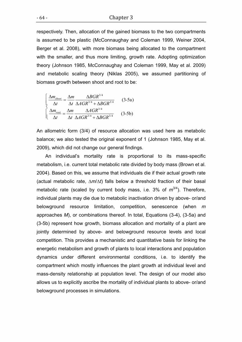
- 64 - Chapter 3

respectively. Then, allocation of the gained biomass to the two compartments

is assumed to be plastic (McConnaughay and Coleman 1999, Weiner 2004,

Berger et al. 2008), with more biomass being allocated to the compartment

with the smaller, and thus more limiting, growth rate. Adopting optimization

theory (Johnson 1985, McConnaughay and Coleman 1999, May et al. 2009)

and metabolic scaling theory (Niklas 2005), we assumed partitioning of

biomass growth between shoot and root to be:

3/4

3/4 3/4

3/4

3/4 3/4

(3-5a)

(3-5b)

shoot

root

m m BGR

t t AGR BGR

m m AGR

t t AGR BGR

An allometric form (3/4) of resource allocation was used here as metabolic

balance; we also tested the original exponent of 1 (Johnson 1985, May et al.

2009), which did not change our general findings.

An individual’s mortality rate is proportional to its mass-specific

metabolism, i.e. current total metabolic rate divided by body mass (Brown et al.

2004). Based on this, we assume that individuals die if their actual growth rate

(actual metabolic rate, ∆m/∆t) falls below a threshold fraction of their basal

metabolic rate (scaled by current body mass, i.e. 3% of m3/4). Therefore,

individual plants may die due to metabolic inactivation driven by above- or/and

belowground resource limitation, competition, senescence (when m

approaches M), or combinations thereof. In total, Equations (3-4), (3-5a) and

(3-5b) represent how growth, biomass allocation and mortality of a plant are

jointly determined by above- and belowground resource levels and local

competition. This provides a mechanistic and quantitative basis for linking the

energetic metabolism and growth of plants to local interactions and population

dynamics under different environmental conditions, i.e. to identify the

compartment which mostly influences the plant growth at individual level and

mass-density relationship at population level. The design of our model also

allows us to explicitly ascribe the mortality of individual plants to above- or/and

belowground processes in simulations.

Chapter 3 - 65 -

3.2.2. Scenarios

In our simulation experiments, we tested high initial densities (104 = 10, 000

individuals per total area), two modes of aboveground (shoot) competition (CAA:

allometric asymmetry, pa = 10; CSS: size symmetry, pa = 1), and two modes of

belowground (root) competition (CAA: allometric asymmetry, pb = 10; CSS: size

symmetry, pb = 1) at three resource-limitation levels for the belowground

compartment (RLb equal to 0, 0.4 and 0.8 representing no, medium and strong

limitation of belowground resources respectively). Simulations for the resulting

nine scenarios were repeated five times, using different random initializations.

We also tested low initial densities (103.5 ≈ 3,163 individuals per total area) and

other combinations of competition parameters, which lead to similar

conclusions as we presented here (Table S1).

3.2.3. Greenhouse experiment

To test the predictions of our model, we carried out a greenhouse experiment

at the research station of Hetzdorf, Dresden University of Technology,

Germany. A common tree species of central Europe, Betula pendula Roth

(silver birch), was chosen because it is fast-growing. The germination

percentage of birch in our controlled pre-test under climate chamber conditions

was 45% (ISTA 1993). Seeds of B. pendula were sown in the pots at two initial

densities (calculated as 0.09g and 0.27g per pot), then two initial seedling

densities with approximately 250 and 750 individuals per pot have been

established, which correspond to 10000 and 33000 plants m-2. Each pot was

filled with a natural mixed spruce forest humus substrate. The plastic pot size

was 20×16.3 cm at top and 17×13.5 cm at bottom with 5 cm in depth.

Consequently, root competition is expected to be very intensive in such

shallow pots (Wilson 1988).

On 11 April 2010, seeds were sown into each pot and covered by a thin

layer of sand against drought damages. We set two nutrient levels, as fertilized

and non-fertilized groups. For the fertilized group, sustained-release fertilizer

was placed uniformly over the ground substance surface in each pot (4.6 g per

pot). In total, we used 40 pots, for two densities, two nutrient levels and ten

replicates. All pots were arranged on benches in the greenhouse, and were

- 66 - Chapter 3

randomly rearranged once per week to avoid possible effects of environmental

heterogeneity. On 28 July 2010, we terminated the planting experiment and

harvested all plants. Self-thinning had largely reduced density of seedlings in

all harvested pots. In order to avoid edge effects, we set up a 7×7 cm subplot

in the center of each pot for measurement. Shoot and root dry biomass were

measured for each individual plant after oven-drying to constant weights at

60°C. Two pots in the fertilization group were lost (one pot in each initial

density), thus 38 pots were evaluated.

3.2.4. Statistical analysis

The mass-density relationship (log-log transformed data of mean biomass vs.

live plant density) has the form log My = log k + γ log N, where My (mean

biomass of either total plants, shoots, or roots) and N (plant density) are the

variables plotted on the ordinate and abscissa, respectively. The constant log k

is the intercept and γ the slope of the regression line (the allometric or scaling

exponent). We used the data of simulated population with high initial density

(i.e. 10,000 individuals per total area) for analysis (the thinning trajectories of

low initial densities were identical to high initial density in simulations; Fig. S1).

Data points were selected a posteriori for linear fits in our simulation

experiment (Weller 1987, Chu et al. 2010): for each scenario, after

density-dependent mortality starts, the data points with surviving plants

between 7,000 and 500 during self-thinning were selected, which excluded the

data points that may cause a non-linearity effect on linear regression. Data

points were fitted by standard major axis regression (SMA, type II model),

which concerns the presence of error in both variables and is widely used to

investigate mass-density relationships (Warton et al. 2006). All statistical

analyses were conducted using R 2.11.1 (R Development Core Team, 2010).

3.3 Results

3.3.1 Individual-based model

Plants allocated more biomass to roots for acquiring belowground resources

(RLb) when these resources became limited. As expected, root : shoot ratio

Chapter 3 - 67 -

(RSR) was significantly higher with belowground resource limitation (ANOVA,

F = 11.48, P < 0.001; Fig. 3.1a). Consequently, belowground competition

among plants became more intense leading to increased mortality (Fig. 3.1b).

This suggests that the relative importance of above- and belowground

competition for the population dynamics varies inversely along a gradient of

belowground resource limitation.

Also, the plasticity of biomass allocation contributes to variable

mass-density patterns (Fig. S1; Table S1). When the mode of competition is

entirely asymmetric (CAA AA , for both above and below ground) and without

resource limitation (RLb=0), the slopes of log mass-log density relationships for

mean total, above- and belowground biomass are all consistent with the

prediction of MST (Fig. 3.2, Table S1). With increasing belowground resource

limitation, the slopes of log mass-log density relationships for belowground

biomass still supports MST but the slopes for aboveground part are

significantly shallower (95% CI do not include -4/3; Fig. 3.2, Table S1).

However, at all resource levels, entirely symmetric competition (CSS SS ) results in

slopes of the log mass-log density relationships significantly shallower than

predicted by MST (95% CI do not include -4/3; Fig. 3.2, Table S1), for both

above- and belowground biomass. This result indicates that the mode of

competition contributed more to altering the mass-density relationship than

biomass allocation did.

In the combination CAA SS without resource limitation (RLb=0, Fig. 3.1b),

aboveground competition had a greater effect on population mortality than

belowground competition because there was no resource limitation. The

allometric exponents were very close to those of the combination CAA AA (95% CI

overlapped; Fig. 3.2, Table S1) and also compatible with prediction of MST (95%

CI include -4/3), but significantly differ from CSS SS (95% CI did not overlap; Fig.

3.2, Table S1). When belowground resources were limited (RLb=0.4), plant

allocated more biomass to belowground parts; the aboveground mass-density

relationship of CAA SS was significantly different from the prediction of MST (95%

CI did not include -4/3) and CAA AA (95% CI did not overlap; Fig. 3.2, Table S1).

However, exponents of belowground showed little variation and were still

consistent with MST (also CAA AA) reflecting that mortality was mainly induced by

asymmetric aboveground competition (Fig. 3.1b).

- 68 - Chapter 3

With further increased belowground resource limitation (RLb=0.8), the

mass-density relationships of CAA SS for mean total, above- and belowground

biomass were very similar to the case of CSS SS (Fig. 3.2, Table S1) and thus

significantly different from the predictions of MST and CAA AA (Fig. 3.2, Table S1).

In this scenario, symmetric belowground competition was the main factor

driving mortality (Fig. 3.1b). This result again demonstrated that the

mass-density relationships are more affected by the mode of competition

independent of which compartment is dominant in terms of growth limitation.

Fig. 3.1 The (a) root:shoot ratio (mean ± 1 SD) and (b) percentage of mortality

induced by above- or belowground competition in simulated plant populations at

different levels of belowground resource limitation, RLb, ranging from 0 (no resource

limitation) to 1 (maximum resource limitation). C with superscript and subscript

indicated the mode of competition for above- and belowground part correspondingly

(AA: allometric asymmetry; SS: size symmetry). Bars in the same group that share

the same letter do not differ significantly (P > 0.05, Holm-Sidak test).

Chapter 3 - 69 -

Fig. 3.2 Slopes of mass-density relationships between the mean total, above- and

belowground biomass and densities in simulated plant populations (log-log

transformed; as estimated by standard major axis; all regressions were significant at

P < 0.0001). RLb defined the level of belowground resource limitation, with its value

ranging from 0 (no resource limitation) to 1 (maximum resource limitation). C with

superscript and subscript indicated the mode of competition for above- and

belowground part correspondingly (AA: allometric asymmetry; SS: size symmetry).

The dotted lines indicate the value of exponent (-4/3) predicted by MST.

3.3.2 Greenhouse experiment

Our greenhouse experiment confirmed the results of the simulation

experiments. For non-fertilized plants the mean RSR of biomass was

significantly higher than for fertilized plants (ANOVA, F = 9.09, P < 0.001; Fig.

3.3). The mass-density relationship varied between fertilization and

non-fertilization treatment (Table S2, Fig. 3.4a). As for fertilized plants, the

slopes of total, above- and belowground log mass-log density relationship

were not significantly different from the prediction of MST (95% CI included

-4/3; Table S2). However, the slopes became shallower in the group of

non-fertilized plants (Fig. 3.4b) and differed significantly from the prediction of

MST (95% CI do not include -4/3; Table S2). The overall pattern of differences

in allometric exponents between fertilization and non-fertilization treatment

(Fig. 3.4b) was similar to the pattern of C AA SS changing along the

resource-limited gradient explored in the simulation experiments (Fig. 3.2)

- 70 - Chapter 3

confirming the dominance change from aboveground (asymmetric) to

belowground (symmetric) competition. Therefore, the importance of

belowground competition as driving force in plant population and communities

is predicted to increase along gradients of decreasing belowground resource

availability, whereas the importance of aboveground competition is predicted

to decrease.

Fig. 3.3 The root:shoot ratio (mean ± 1 SE) of Betula pendula seedlings in

greenhouse experiment with different nutrient treatments and initial densities (L: low

density, H: high density, L+H: combined data). Bars that share the same letter do not

differ significantly (P > 0.05, Holm-Sidak test).

Chapter 3 - 71 -

Fig. 3.4 The mass-density relationships of Betula pendula seedlings in greenhouse

experiment with different nutrient treatments. (a) Relationships between mean total,

above- and belowground biomass and densities (log-log transformed). (b) Slopes of

mass-density relationships between the mean total, above- and belowground

biomass and densities (log-log transformed, as estimated by standard major axis; all

regressions were significant at P < 0.001, 95% CI of the slopes indicated that the

exponents of non-fertilization treatment were statistically different from −4/3).

3.4 Discussion

We presented a two-layer individual-based model that is rooted in metabolic

scaling theory (MST). The purpose of the model was to test whether a generic

model that explicitly represents biomass allocation and different modes of

- 72 - Chapter 3

competition for both above- and belowground compartments would be able to

capture observed variations and patterns in plant mass-density relationships.

In addition to simulation experiments, we conducted a greenhouse experiment

to verify the model’s predictions.

The main finding was that changes in the allometry of plants, induced by

their plasticity of biomass allocation in response to environmental factors, can

alter the relative importance of above- or belowground competition on driving

density-dependent mortality, which affects plant mass-density relationships.

Root competition, which is assumed to be more symmetric, can have a strong

effect on altering the allometric exponent, i.e. flattening plant log mass-log

density relationships (also self-thinning trajectories). Deviations from the

mass-density scaling exponent predicted by MST are thus likely to occur if

competition occurs belowground (symmetric) rather than aboveground

(asymmetric). Consequently, models or theories explaining mass-density

relationships and self-thinning which are solely based on aboveground parts

are unlikely to be appropriate for the cases where belowground processes

predominate (Deng et al. 2006, Berger et al. 2008).

3.4.1. The advantages of using a new mechanistic growth model

It was important that we used a mechanistic growth model derived from MST

rather than a phenomenological growth model, as usually has been done so

far for analyzing biomass-density relationships (e.g., Weiner et al. 2001, Stoll

et al. 2002, Chu et al. 2010). First, our generic growth model is based on the

energy budget of the individuals during growth. It thus captures the salient

features of energy acquisition and allocation to maintain and replace the

existing tissue and the production of new tissue, and relates ontogenetic

growth to metabolic energy at the cellular level (West et al. 2001). This

certainly is an advantage by itself because models driven by “first principles”

are more flexible and usually capture more adaptive responses of individuals

to their environment than phenomenological models, which are statistically

fitted to existing data (Grimm and Railsback 2005, Martin et al. 2012). Second,

in contrast to previous models (Wyszomirski et al. 1999, Weiner et al. 2001,

Stoll et al. 2002, Chu et al. 2010), our model is able to simultaneously explain

Chapter 3 - 73 -

the observed variation in both root-shoot allocation patterns and mass-density

relationships.

It is worth noting that an association of the scaling exponents with root :

shoot ratios (RSR) predicted by our model matched the observed values of

natural vegetations along a precipitation gradient in China very well. Deng et al.

(2006) found that with drought severity increasing, the mean RSR of plant dry

biomass increased approximately from 1 to 2 (RSR±SD: 0.92±0.31, 1.92±1.42

and 2.18±1.61) and the scaling exponent of plant total biomass-density

relationship changed from -1.33 to -1.27 correspondingly (-1.33, -1.28 and

-1.27). In our model, we found very similar associations between RSR and

scaling exponent (Table S1; e.g., C AA SS : RLb=0, RSR±SD=1.09±0.03,

Slope=-1.36; RLb=0.4, RSR±SD=1.66±0.16, Slope=-1.29), which are

statistically identical to the empirical results (P > 0.05, Holm-Sidak test).

3.4.2. Above- and belowground competition

Why do the predictions of MST on plant mass-density relationship often turn

out to be correct? The principal assumption of energy equivalence in MST

implies that light is the limiting factor and competition is a canopy-packing

process among plants (Enquist et al. 1998, Reynolds and Ford 2005, Deng et

al. 2006). If then in benign environments only aboveground biomass is

measured, as in most empirical studies, it is to be expected that we obtain the

slope of -4/3 (scaling exponent) as shown in our model.

Our results imply the importance of adaptive behaviours of plants for

system-level properties like biomass-density relationship (Grimm and

Railsback 2005, Grimm et al. 2005). With “adaptive behaviour” we refer to

morphological and physiological plasticity that allows plants to adapt to

changing biotic and abiotic environmental conditions (Weiner 2004, Berger et

al. 2008, Schiffers et al. 2011). It is recognized that features of vegetation can

change in drought or oligotrophic environments (Deng et al. 2006). Based on

optimization theory, plants compete primarily for limited belowground

resources in those environments, which can cause an increase of RSR as well

as root space, but a decrease in cover where plant canopies are not closed

(Deng et al. 2006). In analogy to Liebig’s law of limiting factors, belowground

- 74 - Chapter 3

competition can overtake aboveground competition and becomes dominant in

these situations. Consequently, adaptive behaviour not only alters the way

plants grow but also their mode of competition.

Empirical experiments show that slopes of log mass-log density

relationship are manifestly shallower under severe water stress (Deng et al.

2006, Liu et al. 2006) and low nutrient levels (reviewed in Morris 2003). Our

model and greenhouse experiments confirm these results. As demonstrated,

the mode of competition played a more important role for the plant

mass-density relationship.

3.4.3. Asymmetric vs. symmetric competition

With symmetric competition, resource acquisition is more evenly distributed

among interacting plants, so that competitive suppression and the

corresponding onset of mortality are delayed (Stoll et al. 2002). Consequently,

even at high densities plants can still survive and grow (Hautier et al. 2009,

Lamb et al. 2009). This leads to the shallower self-thinning lines as has been

proven in several studies (Chu et al. 2010, Lin et al. in revision).

Accordingly, one should also expect that slopes become shallower if

aboveground competition is less asymmetric. This was indeed observed for

low light conditions (Lonsdale and Watkinson 1982, Westoby 1984, Dunn and

Sharitz 1990), where plants often show flexible shoot morphology and grow

taller instead of wider, and competition was considered more symmetric

(Schwinning and Weiner 1998, Stoll et al. 2002).

However, some researchers proposed that size-asymmetric (light)

competition is more important for explaining the deviations predicted by MST

in forests (Coomes and Allen 2009; Coomes et al. 2011). At first glance, this

seems to be in contrast to our findings here, but this is not the case because

those studies focused on individual’s diameter growth. Asymmetric competition

from larger neighbours can highly affect the growth of smaller individuals

before they die. Thus, for these individuals, asymmetric competition is more

important than the relationships predicted by MST. In contrast, we here

focused on the biomass and density of surviving plants.

It is noteworthy to mention that it also has been surmised that

Chapter 3 - 75 -

belowground competition might be rather asymmetric in heterogeneous

resource conditions (Schwinning and Weiner 1998, Fransen et al. 2001,

Rajaniemi 2003, Rewald and Leuschner 2009), though the experimental

evidence for asymmetric belowground competition is scarce (Rajaniemi 2003,

von Wettberg and Weiner 2003, Rewald and Leuschner 2009). Our model and

greenhouse experiment, nevertheless, confirm the majority of empirical

experiments which suggest that belowground competition is more symmetric.

We conclude that an appropriate evaluation of the mode of competition should

not only consider environmental heterogeneity and species-specific ecological

traits of plants (Schwinning and Weiner 1998, Rajaniemi 2003, Pretzsch 2006,

Rewald and Leuschner 2009), but also the interaction between above- and

belowground competition (Cahill 2002).

Conclusion

It seems that Liebig’s law even applies, in a generalized sense, to the debate

about whether or not MST is a universally valid and relevant theory. Deviation

in observed plant mass-density relationships indicates that MST is less general

than originally thought. Our findings confirm that MST by itself applies to

individual organisms, but not necessarily to populations or ecosystems (Lin et

al. in revision). System-level features of ecological systems may be

constrained by individual metabolism, which is taken into account in MST, or

by ecological factors beyond the individual, i.e. the type of limiting resource

and the mode of competition among con-specifics. The overall claim that MST

provides a universal and mechanistic basis for quantitatively linking the

energetic metabolism of individuals to ecological community dynamics is thus

neither completely right nor wrong: the real question is when and which factors

dominate in a given situation.

In addition to previous studies, which do not address the linkage between

aboveground and belowground competition explicitly, the most important

conclusion of our study is that changes in biomass allocation patterns can

modify ecological mechanisms and subsequently the constraints which MST

sets. The observed variation in mass-density relationships represents changes

in the dominance of the most limiting factor in a given ecological context. This

- 76 - Chapter 3

has important implications, e.g., for using allometry-based simulation models

to predict carbon storage and sequestration in plant systems. Taking into

account not only the visible aboveground competition, but also the invisible

belowground competition, is thus critical for many forests and eco-regions.

Acknowledgements

We thank Angelika Körner, Christine Lemke, Antje Karge, Heinz Wolf and

Sven Wagner for their kind help. We are particularly grateful to Jacob Weiner

who showed us once again the beauty and seriousness science. The first

author was supported by Helmholtz Impulse and Networking Fund through

Helmholtz Interdisciplinary Graduate School for Environmental Research

(HIGRADE).

References

Berger, U., C. Piou, K. Schiffers, and V. Grimm. 2008. Competition among plants: concepts, individual-based modelling approaches, and a proposal for a future research strategy. Perspectives in Plant Ecology, Evolution and Systematics 9:121–135.

Brown, J. H., J. F. Gillooly, A. P. Allen, V. M. Savage, and G. B. West. 2004. Toward a metabolic theory of ecology. Ecology 85:1771–1789.

Cahill J. F., Jr. and B. B. Casper. 2000. Investigating the relationship between neighbor root biomass and belowground competition: field evidence for symmetric competition belowground. Oikos 90:311–320.

Cahill J. F., Jr. 2002. Interactions between root and shoot competition vary among species. Oikos 99:101–112.

Casper, B. B., H. J. Schenk, and R. B. Jackson. 2003. Defining a plant’s belowground zone of influence. Ecology 84:2313–2321.

Cheng, D. L., and K. J. Niklas. 2007. Above- and belowground biomass relationships across 1534 forested communities. Annals of botany 99:95–102.

Chu, C. J., J. Weiner, F. T. Maestre, Y. S. Wang, C. Morris, S. Xiao, J. L. Yuan, G. Z. Du, and G. Wang. 2010. Effects of positive interactions, size symmetry of competition and abiotic stress on self-thinning in simulated plant populations. Annals of botany 106:647–652.

Coomes, D. A. 2006. Challenges to the generality of WBE theory. Trends in ecology & evolution 21:593–596.

Coomes, D. A., and R. B. Allen. 2009. Testing the metabolic scaling theory of tree growth. Journal of Ecology 97:1369–1373.

Coomes, D. A., E. R. Lines, and R. B. Allen. 2011. Moving on from Metabolic Scaling Theory: hierarchical models of tree growth and asymmetric competition for light. Journal of Ecology 99:748–756.

Deng, J. M., G. X. Wang, E. C. Morris, X. P. Wei, D. X. Li, B. M. Chen, C. M. Zhao, J. Liu, and Y. Wang. 2006. Plant mass–density relationship along a moisture gradient in north‐west China. Journal of Ecology 94:953–958.

Dunn, C. P., and R. R. Sharitz. 1990. The relationship of light and plant geometry to self‐thinning of an aquatic annual herb, Murdannia keisak (Commelinaceae). New Phytologist 115:559–565.


http://tu-dresden.de/die_tu_dresden/fakultaeten/fakultaet_forst_geo_und_hydrowissenschaften/fachrichtung_forstwissenschaften/institute/wb/waldbau/dateien/wagner

Chapter 3 - 77 -

general quantitative theory linking plant form and function from cells to ecosystems. Tree physiology 22:1045–1064.

Enquist, B. J., J. H. Brown, and G. B. West. 1998. Allometric scaling of plant energetics and population density. Nature 395:163–165.

Enquist, B. J., and K. J. Niklas. 2001. Invariant scaling relations across tree-dominated communities. Nature 410:655–660.

Enquist, B. J., G. B. West, and J. H. Brown. 2009. Extensions and evaluations of a general quantitative theory of forest structure and dynamics. Proceedings of the National Academy of Sciences, USA 106:7046–7051.

Fransen, B., H. de Kroon, and F. Berendse. 2001. Soil nutrient heterogeneity alters competition between two perennial grass species. Ecology 82:2534–2546.

Grimm, V., U. Berger, F. Bastiansen, S. Eliassen, V. Ginot, J. Giske, J. Goss-Custard, T. Grand, S. K. Heinz, and G. Huse. 2006. A standard protocol for describing individual-based and agent-based models. Ecological Modelling 198:115–126.

Grimm, V., U. Berger, D. L. DeAngelis, J. G. Polhill, J. Giske, and S. F. Railsback. 2010. The ODD protocol: A review and first update. Ecological Modelling 221:2760–2768.

Grimm, V., and S. F. Railsback. 2005. Individual-based modelling and ecology. Princeton University Press, USA

Grimm, V., E. Revilla, U. Berger, F. Jeltsch, W. M. Mooij, S. F. Railsback, H. H. Thulke, J. Weiner, T. Wiegand, and D. L. DeAngelis. 2005. Pattern-oriented modelling of agent-based complex systems: lessons from ecology. Science 310:987–991.

Hautier, Y., P. A. Niklaus, and A. Hector. 2009. Competition for light causes plant biodiversity loss after eutrophication. Science 324:636–638.

ISTA. 1993. International rules for seed testing. Seed Science and Technology 21:1–288. Johnson, I. R. 1985. A model of the partitioning of growth between the shoots and roots of

vegetative plants. Annals of Botany 55:421–431. Lamb, E. G., S. W. Kembel, and J. F. Cahill Jr. 2009. Shoot, but not root, competition

reduces community diversity in experimental mesocosms. Journal of Ecology 97:155–163.

Lin, Y., Berger, U., Grimm, V., and Q. R. Ji. 2012. Differences between symmetric and asymmetric facilitation matter: exploring the interplay between different modes of positive and negative plant interactions. Journal of Ecology DOI: 10.1111/j.1365-2745.2012.02019.x

Liu, J., L. Wei, C. M. Wang, G. X., and X. P. Wei. 2006. Effect of Water Deficit on Self‐thinning Line in Spring Wheat (Triticum aestivum L.) Populations. Journal of Integrative Plant Biology 48:415–419.

Lonsdale, W. M., and A. R. Watkinson. 1982. Light and self-thinning. New Phytologist:431–445.

Martin, B. T., E. I. Zimmer, V. Grimm, and T. Jager. 2012. Dynamic Energy Budget theory meets individual-based modelling: a generic and accessible implementation. Methods in Ecology and Evolution 3:445–449.

May, F., V. Grimm, and F. Jeltsch. 2009. Reversed effects of grazing on plant diversity: the role of below‐ground competition and size symmetry. Oikos 118:1830–1843.

McConnaughay, K. D. M., and J. S. Coleman. 1999. Biomass allocation in plants: ontogeny or optimality? A test along three resource gradients. Ecology 80:2581–2593.

Morris, E. C. 2003. How does fertility of the substrate affect intraspecific competition? Evidence and synthesis from self‐thinning. Ecological Research 18:287–305.

Niklas, K. J. 2005. Modelling below-and aboveground biomass for non-woody and woody plants. Annals of Botany 95:315–321.

O’Brien, E. E., J. S. Brown, and J. D. Moll. 2007. Roots in space: a spatially explicit model for belowground competition in plants. Proceedings of the Royal Society B: Biological Sciences 274:929–935.

R Development Core Team (2010) R: a language and environment for statistical computing. R Foundation for Statistical Computing, URL http://www.R-project.org. Last accessed 17 February 2012.

http://www.sciencedirect.com/science?_ob=RedirectURL&_method=externObjLink&_locator=url&_issn=00029297&_origin=article&_zone=art_page&_plusSign=%2B&_targetURL=http%253A%252F%252Fwww.R-project.org

- 78 - Chapter 3

Pretzsch, H. 2006. Species-specific allometric scaling under self-thinning: evidence from long-term plots in forest stands. Oecologia 146:572–583.

Rajaniemi, T. K. 2003. Evidence for size asymmetry of belowground competition. Basic and Applied Ecology 4:239–247.

Rewald, B., and C. Leuschner. 2009. Does root competition asymmetry increase with water availability? Plant Ecology & Diversity 2:255–264.

Reynolds, J. H., and E. D. Ford. 2005. Improving competition representation in theoretical models of self‐thinning: a critical review. Journal of Ecology 93:362–372.

Savage, V. M., L. P. Bentley, B. J. Enquist, J. S. Sperry, D. D. Smith, P. B. Reich, and E. I. von Allmen. 2010. Hydraulic trade-offs and space filling enable better predictions of vascular structure and function in plants. Proceedings of the National Academy of Sciences, USA 107:22722–22727.

Schiffers, K., K. Tielbörger, B. Tietjen, and F. Jeltsch. 2011. Root plasticity buffers competition among plants: theory meets experimental data. Ecology 92:610–620.

Schwinning, S., and J. Weiner. 1998. Mechanisms determining the degree of size asymmetry in competition among plants. Oecologia 113:447–455.

Stoll, P., J. Weiner, H. Muller-Landau, E. Müller, and T. Hara. 2002. Size symmetry of competition alters biomass–density relationships. Proceedings of the Royal Society of London. Series B: Biological Sciences 269:2191–2195.

Tilman, D. 1988. Plant strategies and the dynamics and structure of plant communities. Princeton University Press, USA

Warton, D. I., I. J. Wright, D. S. Falster, and M. Westoby. 2006. Bivariate line‐fitting methods for allometry. Biological Reviews 81:259–291.

Weiner, J. 2004. Allocation, plasticity and allometry in plants. Perspectives in Plant Ecology, Evolution and Systematics 6:207–215.

Weiner, J., and R. P. Freckleton. 2010. Constant final yield. Annual Review of Ecology, Evolution, and Systematics 41:173–192.

Weiner, J., P. Stoll, H. Muller‐Landau, and A. Jasentuliyana. 2001. The effects of density, spatial pattern, and competitive symmetry on size variation in simulated plant populations. The American Naturalist 158:438–450.

Weller, D. E. 1987. Self-thinning exponent correlated with allometric measures of plant geometry. Ecology 68:813–821.

West, G. B., J. H. Brown, and B. J. Enquist. 1999. A general model for the structure, function, and allometry of plant vascular systems. Nature 400:664–667.

West, G. B., J. H. Brown, and B. J. Enquist. 2001. A general model for ontogenetic growth. Nature 413:628–631.

Westoby, M. 1984. The self-thinning rule. Advances in Ecological Research 14:167–225. von Wettberg, E. J., and J. Weiner. 2003. Larger Triticum aestivum plants do not preempt

nutrient-rich patches in a glasshouse experiment. Plant Ecology 169:85–92. Wilensky, U. (1999). NetLogo. Center for Connected Learning and Computer-Based

Modelling, Northwestern University. Available at: http://ccl.northwestern.edu/netlogo/. Last accessed 17 February 2012.

Wilson, J. B. 1988. Shoot competition and root competition. Journal of Applied Ecology 25:279–296.

Wyszomirski, T. 1983. Simulation model of the growth of competing individuals of a plant population. Ekologia Polska 31.

Wyszomirski, T., I. Wyszomirska, and I. Jarzyna. 1999. Simple mechanisms of size distribution dynamics in crowded and uncrowded virtual monocultures. Ecological Modelling 115:253–273.

Yoda, T. Kira, H. Ogawa, and K. Hozumi. 1963. Self-thinning in overcrowded pure stands under cultivated and natural conditions (Intraspecific competition among higher plants XI). Journal of Biology, Osaka City University 14:107–129.

Chapter 3 - 79 -


ODD protocol – model description of two-layer pi model




1. Purpose

The aim of this model is to evaluate the multiple effects of the mode of

competition (above- and belowground part) and resource limitation on

regulating plant population dynamics, specifically on mass-density

relationships (self-thinning trajectories) and density-dependent mortality. In

particular, we test whether interactions on individual plant level can alter the

slope and intercept of the log mass-log density relationship under different

environmental conditions. The model does not represent specific species, but

generic ones.

2. Entities, state variables, and scales


A1). Plants are characterized by the following state variables: initial growth rate,

initial biomass, maximum biomass (asymptotic biomass), current biomass

(both shoot and root) and their position, i.e. coordinates of the stem. Each

individual plant has its own circular zone-of-influence (ZOI) for both above- and

belowground compartment. The pair of ZOIs stand for the physical space

occupied by a plant’s shoot and root respectively, and represents the energy

and resources potentially available to this plant for above- and belowground

part, which ZOIs are allometrically related to its shoot and root mass separately.

Neighbouring plants only compete for the resources when their above- or

belowground ZOIs are overlapping.



torus world with a size of 200 × 200 patches (Grimm & Railsback 2005), and

each patch represents 0.25 cm2 in reality. The state of each patch is

characterized by its resource availability. We use a homogeneous environment

here as all patches have the same, and constant, degree of resource limitation

for both above- and belowground part. One time step in the model represents

approximately one week for simulated plants.

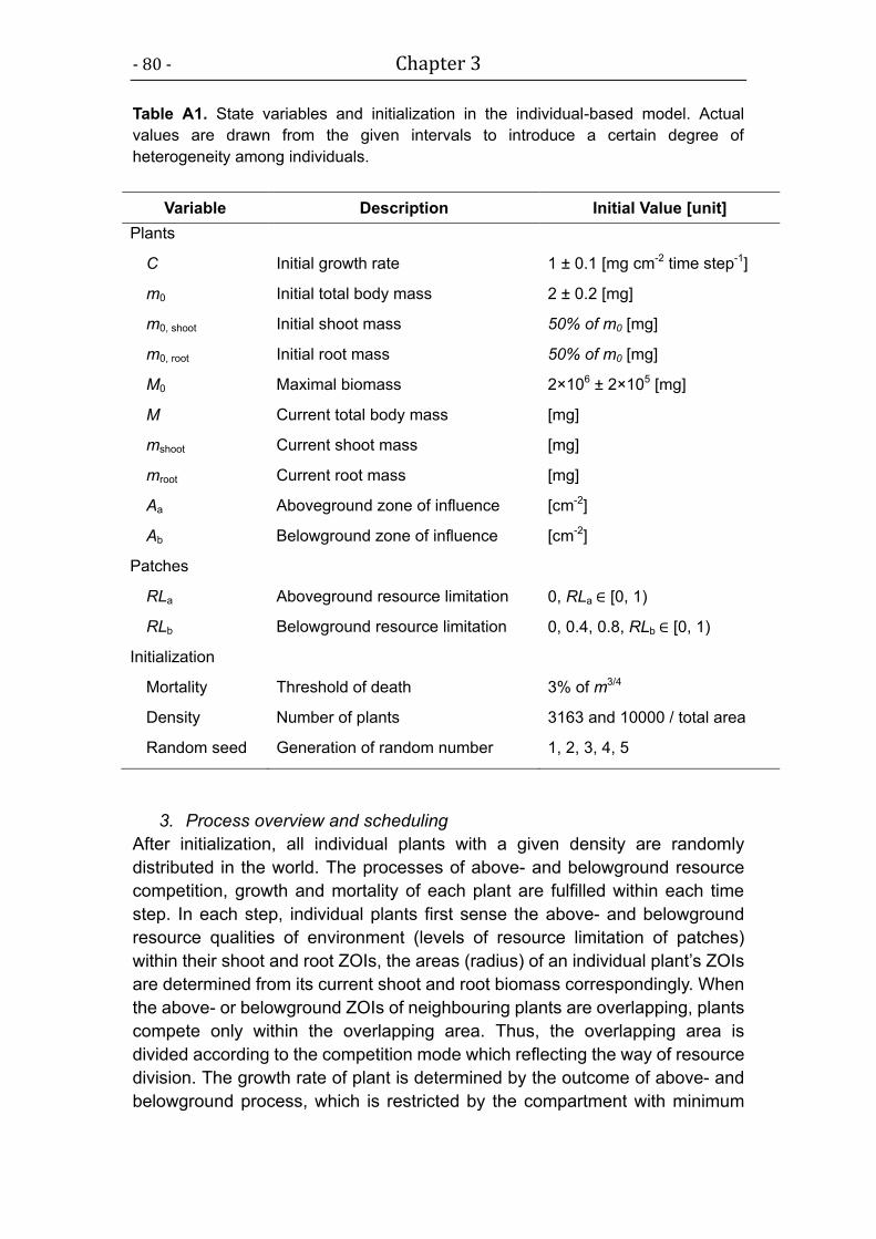
- 80 - Chapter 3





Plants

C Initial growth rate 1 ± 0.1 [mg cm-2 time step-1]

m0 Initial total body mass 2 ± 0.2 [mg]

m0, shoot Initial shoot mass 50% of m0 [mg]

m0, root Initial root mass 50% of m0 [mg]

M0 Maximal biomass 2×106 ± 2×105 [mg]

M Current total body mass [mg]

mshoot Current shoot mass [mg]

mroot Current root mass [mg]

Aa Aboveground zone of influence [cm-2]

Ab Belowground zone of influence [cm-2]

Patches

RLa Aboveground resource limitation 0, RLa ∈ [0, 1)

RLb Belowground resource limitation 0, 0.4, 0.8, RLb ∈ [0, 1)

Initialization


Density Number of plants 3163 and 10000 / total area

Random seed Generation of random number 1, 2, 3, 4, 5

3. Process overview and scheduling


distributed in the world. The processes of above- and belowground resource

competition, growth and mortality of each plant are fulfilled within each time

step. In each step, individual plants first sense the above- and belowground

resource qualities of environment (levels of resource limitation of patches)

within their shoot and root ZOIs, the areas (radius) of an individual plant’s ZOIs

are determined from its current shoot and root biomass correspondingly. When

the above- or belowground ZOIs of neighbouring plants are overlapping, plants

compete only within the overlapping area. Thus, the overlapping area is

divided according to the competition mode which reflecting the way of resource

division. The growth rate of plant is determined by the outcome of above- and

belowground process, which is restricted by the compartment with minimum

Chapter 3 - 81 -

resource uptake rate according to growth function. The synthesized biomass is

allocated to shoot and root optimally which follows the rule of functional

balanced growth (Niklas 2005; May et al. 2009). Plants with growth rates

falling below a threshold die and are removed immediately. The state variables

of the plants are synchronously updated within the subroutines, i.e. changes to

state variables are updated only after all individuals have been processed

(Grimm & Railsback 2005).

4. Design concepts



ZOI approach, with the effects of different modes of competition for both

above- and belowground compartment and resource limitation.


relationship or self-thinning trajectories, size distribution and spatial distribution,

emerge from the interaction of individual plants with their neighbours and the

resource level of their abiotic environment.

Interaction: Individual plants interact via shoot and root competition for

resources in the overlapping area of their ZOIs.

Stochasticity: Initial growth rate, initial biomass (for shoot and root

respectively), maximum biomass and initial position of plants are randomly

taken from the intervals given in Table 1. This introduces a certain level of

heterogeneity among individual characteristics to take into account that real

plants are never exactly identical.

Observation: Population size, shoot and root biomass of each plant, and mean

biomass of all living plants are the main observations.

5. Initialization

Initially, individual plants are randomly distributed according to the chosen

initial density. Resources are spatially and temporally constant. Each plant has

an initial biomass (m0), initial shoot and root biomass (m0, shoot and m0, root),

maximal biomass (M) and initial growth rate (c) drawn from truncated normal

distributions with average and intervals given in Table 1.

6. Input



7. Submodels

One layer model – Plant growth, resource limitation and competition

In our individual-based model the plant’s ZOI, A, stands for the physical space

occupied by the plant and represents the energy and resources potentially



- 82 - Chapter 3

constant. Since plant growth in our simulation is discrete, therefore equation

(3-1) can be rewritten as

∆m/∆t = cA[ 1 – ( m / M0)1/4 ] (A1)

where c=ac0, is the initial growth rates in units of mass per area and time

interval. For simplicity, we choose 1 ± 0.1 in our model.

Resource limitation and competition usually cause a reduction of resource

availability for plants. We therefore represent resource limitation via a

dimensionless efficiency factor or index, fR, for different levels of resource

availability. Resource competition is incorporated by using a dimensionless

competition factor or index, fp, leading to

∆m/∆t = fRfpcA[ 1 – ( m / M)1/4 ] (A2)

where M=(fRfp)4M0 is the maximum body size with resource limitation and

competition.

The efficiency factor fR, can take different forms depending on the

characteristics and level of the limiting resource. For simplification, we use a

linear form here, i.e. fR = 1–RL, where RL indicates the level of resource

limitation, with its value ranging from 0 (no resource limitation) to 1 (maximum

resource limitation).

As for competition, the modes of resource-mediated competition among





different modes of competition explicitly, we describe the competitive index fp

as

,1

1

( ) /o

j

pn i

p no o knk p

jj

mf A A A

m

(A3)

This factor thus refers to the fraction of resources available in the area

which plant i could obtain after a loss of potential resources due to areas

overlapped by neighbours of sizes mj (Schwinning and Weiner 1998). Ano is

the area not overlapping with neighbours, Ao,k denotes the no areas

overlapping with nj different neighbours. Parameter p determines the mode of


(p approaching infinity; for details and examples see Figure A2).

Chapter 3 - 83 -

Figure A2. An example of calculating the interactive indexes (Eqns A3) with

different modes of competition and facilitation in an individual-based model as

a way of dividing plants’ ZOI (zone-of-influence). Three plants with sizes m1,

m2 and m3 are interacting in this example. For plant 1, its ZOI (A) was divided

into four parts: Ano, the area not overlapping with the other two plants; Ao,1, the

area overlapping with plant 2; Ao,2, the area overlapping with plants 2 and 3;

Ao,3, the area overlapping with plant 3. Then the actual area that plant 1 can

take from Ao,1 is

1 1,1 ,12

1 21

p p

o o p pp

jj

m mA A

m mm

For Ao,2,

1 1,2 ,23

1 2 31

p p

o o p p pp

jj

m mA A

m m mm

And for Ao,3,

1 1,3 ,32

1 31

p p

o o p pp

jj

m mA A

m mm

Therefore, the competitive index for plant 1 is:

Where 3/4

1 0/A m c

Two layer model – Shoot versus root competition, biomass allocation and

mortality

Because competition among plants can occurs at both above- and

belowground simultaneously, the relative importance of shoot versus root

competition and their ZOI can varies depending on the environmental factors

(Deng et al. 2006, May et al. 2009). Therefore, the one layer model however

cannot properly represent this property. We developed the two layer

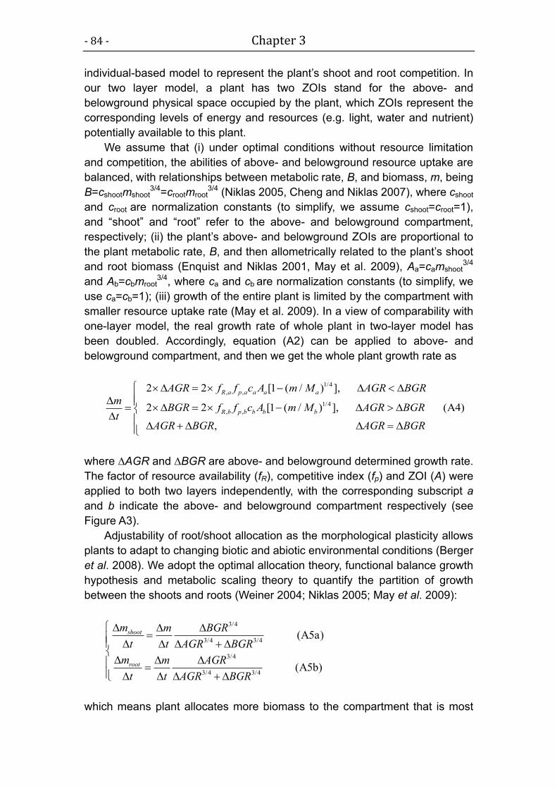
- 84 - Chapter 3

individual-based model to represent the plant’s shoot and root competition. In

our two layer model, a plant has two ZOIs stand for the above- and

belowground physical space occupied by the plant, which ZOIs represent the

corresponding levels of energy and resources (e.g. light, water and nutrient)

potentially available to this plant.

We assume that (i) under optimal conditions without resource limitation

and competition, the abilities of above- and belowground resource uptake are

balanced, with relationships between metabolic rate, B, and biomass, m, being

B=cshootmshoot3/4=crootmroot

3/4 (Niklas 2005, Cheng and Niklas 2007), where cshoot

and croot are normalization constants (to simplify, we assume cshoot=croot=1),

and “shoot” and “root” refer to the above- and belowground compartment,

respectively; (ii) the plant’s above- and belowground ZOIs are proportional to

the plant metabolic rate, B, and then allometrically related to the plant’s shoot

and root biomass (Enquist and Niklas 2001, May et al. 2009), Aa=camshoot3/4

and Ab=cbmroot3/4, where ca and cb are normalization constants (to simplify, we

use ca=cb=1); (iii) growth of the entire plant is limited by the compartment with

smaller resource uptake rate (May et al. 2009). In a view of comparability with

one-layer model, the real growth rate of whole plant in two-layer model has

been doubled. Accordingly, equation (A2) can be applied to above- and

belowground compartment, and then we get the whole plant growth rate as

1/4

, ,

1/4

, ,

2 2 [1 ( / ) ],

2 2 [1 ( / ) ], (A4)

,

R a p a a a a

R b p b b b b

AGR f f c A m M AGR BGR

mBGR f f c A m M AGR BGR

tAGR BGR AGR BGR

where ∆AGR and ∆BGR are above- and belowground determined growth rate.

The factor of resource availability (fR), competitive index (fp) and ZOI (A) were

applied to both two layers independently, with the corresponding subscript a

and b indicate the above- and belowground compartment respectively (see

Figure A3).

Adjustability of root/shoot allocation as the morphological plasticity allows

plants to adapt to changing biotic and abiotic environmental conditions (Berger

et al. 2008). We adopt the optimal allocation theory, functional balance growth

hypothesis and metabolic scaling theory to quantify the partition of growth

between the shoots and roots (Weiner 2004; Niklas 2005; May et al. 2009):

3/4

3/4 3/4

3/4

3/4 3/4

(A5a)

(A5b)

shoot

root

m m BGR

t t AGR BGR

m m AGR

t t AGR BGR

which means plant allocates more biomass to the compartment that is most

Chapter 3 - 85 -

limiting growth for increasing its uptake of resource. An allometric form (3/4) of resources allocation was used here as metabolic balance, we also tested the original allocation of linearity which only lead to a small difference on root/shoot ratio but do not change our general findings.

An individual’s mortality rate is proportional to its mass-specific

metabolism (as current total metabolic rate divide by body mass; Brown et al.

2004). Based on this, we assume that individuals die if their actual growth rate

(∆m/∆t, represent actual metabolic rate) falls below a threshold of their basal

metabolic rate (allometrically scaled with body mass), i.e. 3% of m3/4.

Therefore, individual plants may die due to metabolic inactivation driven by

above- or/and belowground resource limitation, competition, senescence

(when m approaches M) or combinations thereof. This provides a more

realistic representation of relevant ecological process than in previous models

(Stoll et al. 2002; Chu et al. 2009, 2010). In addition, we are able to ascribe the

mortality of individual plants to above- or belowground process explicitly.

In total, equations (A4), (A5a) and (A5b) clearly showed how a plant’s

growth, biomass allocation and mortality are jointly determined by above- and

belowground resource level and local competition.

Figure A3. A visual illustration of the two-layer zone-of-influence (ZOI) approach

including both above- and belowground competition. The above- and belowground

ZOIs (green: aboveground, gray: belowground) are allometrically related to the plant

shoot and root biomass, respectively. Plants only compete for the resources in

overlapped areas with their neighbours which can occur independently at above- and

belowground compartment (arrows indicate the overlapped area of aboveground

competition).

- 86 - Chapter 3

References

Berger, U., Piou, C., Schiffers, K. & Grimm, V. (2008). Competition among plants: Concepts, individual-based modelling approaches, and a proposal for a future research strategy. Perspect. Plant Ecol., 9, 121-135.

Brown, J.H., Gillooly, J.F., Allen, A.P., Savage, V.M. & West, G.B. (2004). Toward a metabolic theory of ecology. Ecology, 85, 1771-1789.

Chu, C.J., Weiner, J., Maestre, FT, Xiao, S., Wang, Y.-S., Li, Q., Yuan, J.L., Zhao, L.Q., Ren, Z.W. and Wang, G.(2009), Positive interactions can increase size inequality in plant populations. J. Ecol., 97, 1401–1407

Chu, C.J., Weiner, J., Maestre, F.T., Wang, Y.S., Morris, C., Xiao, S. et al. (2010). Effects of positive interactions, size symmetry of competition and abiotic stress on self-thinning in simulated plant populations. Ann. Bot., 106, 647-652.

Deng, J.M., Wang, G.X., Morris, E.C., Wei, X.P., Li, D.X., Chen, B.M. et al. (2006). Plant mass-density relationship along a moisture gradient in north-west China. J. Ecol., 94, 953–958.

Enquist, B.J. (2002). Universal scaling in tree and vascular plant allometry: toward a general quantitative theory linking plant form and function from cells to ecosystems. Tree Physiol., 22, 1045-1064.

Enquist, B.J. & Niklas, K.J. (2001). Invariant scaling relations across tree-dominated communities. Nature, 410, 655-660.

Enquist, B.J., West, G.B. & Brown, J.H. (2009). Extensions and evaluations of a general quantitative theory of forest structure and dynamics. Proc. Natl Acad. Sci. USA., 106, 7046-7051.

Grimm, V., Berger, U., Bastiansen, F., Eliassen, S., Ginot, V., Giske, J. et al. (2006). A standard protocol for describing individual-based and agent-based models. Ecol. Model., 198, 115-126.

Grimm, V., Berger, U., DeAngelis, D.L., Polhill, J.G., Giske, J. & Railsback, S.F. (2010). The ODD protocol: A review and first update. Ecol. Model.. 221, 2760-2768.

Grimm, V. & Railsback, S.F. (2005). Individual-based modeling and ecology. Princeton University Press, Princeton and Oxford.

Hou, C., Zuo, W., Moses, M.E., Woodruff, W.H., Brown, J.H. & West, G.B. (2008). Energy uptake and allocation during ontogeny. Science, 322, 736-739.

Lambers, H., Chapin, F.S. & Pons, T.L. (2008). Plant physiological ecology. 2nd edition. Springer Verlag, New York, pp. 134–143.

Maestre, F.T., Callaway, R.M., Valladares, F. & Lortie, C.J. (2009). Refining the stress-gradient hypothesis for competition and facilitation in plant communities. J. Ecol., 97, 199–205.

May, F., Grimm, V. & Jeltsch, F. (2009). Reversed effects of grazing on plant diversity: the role of below-ground competition and size symmetry. Oikos, 118, 1830–1843.

Molofsky, J. & Bever, J.D. (2002). A novel theory to explain species diversity in landscapes: positive frequency dependence and habitat suitability. Proc. R. Soc. Lond., B, Biol. Sci., 269, 2389–2393.

Molofsky, J., Bever, J.D. & Antonovics, J. (2001). Coexistence under positive frequency dependence. Proc. R. Soc. Lond., B, Biol. Sci., 2001, 268–277.

Niklas, K.J. (2005). Modelling below-and above-ground biomass for non-woody and woody plants. Ann. Bot., 95, 315-321.

Niklas, K.J. & Enquist, B.J. (2001). Invariant scaling relationships for interspecific plant biomass production rates and body size. Proc. Natl Acad. Sci. USA., 98, 2922-2927.

Price, C.A., Enquist, B.J. & Savage, V.M. (2007). A general model for allometric covariation in botanical form and function. Proc. Natl Acad. Sci. USA., 104, 13204-13209.

Sack, L., Maranon, T., Grubb, P.J., Enquist, B.J. & Niklas, K.J. (2002). Global allocation rules for patterns of biomass partitioning. Science, 296, 1923a.

Schwinning, S. & Weiner, J. (1998). Mechanisms determining the degree of size asymmetry in competition among plants. Oecologia, 113, 447-455.

Chapter 3 - 87 -

Stoll, P., Weiner, J., Muller-Landau, H., Müller, E. & Hara, T. (2002). Size symmetry of competition alters biomass–density relationships. Proc. R. Soc. Lond. B: Biol. Sci., 269, 2191-2195.

Travis, J.M.J., Brooker, R.W., Clark, E.J. & Dytham, C. (2006). The distribution of positive and negative species interactions across environmental gradients on a dual-lattice model. J. Theor. Biol., 241, 896–902.

Weiner, J., Stoll, P., Muller-Landau, H. & Jasentuliyana, A. (2001). The effects of density, spatial pattern, and competitive symmetry on size variation in simulated plant populations. The American Naturalist, 158, 438-450.

Weiner, J. (2004). Allocation, plasticity and allometry in plants. Perspectives in Plant Ecology, Evolution and Systematics, 6, 207-215.

West, G.B., Brown, J.H. & Enquist, B.J. (1999). A general model for the structure and allometry of plant vascular systems. Nature, 400, 664-667.

West, G.B., Brown, J.H. & Enquist, B.J. (2001). A general model for ontogenetic growth. Nature, 413, 628-631.

West, G.B., Enquist, B.J. & Brown, J.H. (2009). A general quantitative theory of forest structure and dynamics. Proc. Natl Acad. Sci., 106, 7040-7045.

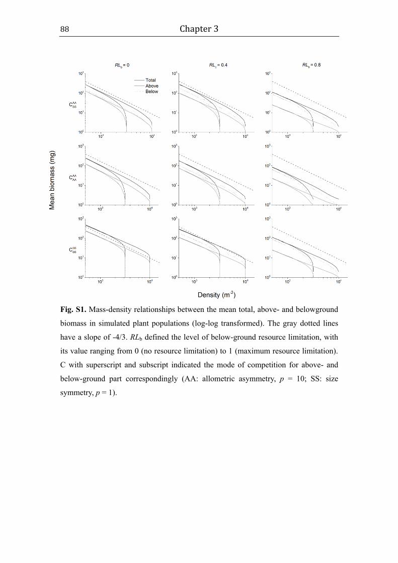
88 Chapter 3

Fig. S1. Mass-density relationships between the mean total, above- and belowground

biomass in simulated plant populations (log-log transformed). The gray dotted lines

have a slope of -4/3. RLb defined the level of below-ground resource limitation, with

its value ranging from 0 (no resource limitation) to 1 (maximum resource limitation).

C with superscript and subscript indicated the mode of competition for above- and

below-ground part correspondingly (AA: allometric asymmetry, p = 10; SS: size

symmetry, p = 1).

Chapter 3 89

Table S1. Slopes and intercepts of mass-density relationships between the mean total,

above- and belowground biomass in simulated plant populations (log-log transformed;

as estimated by standard major axis regression). RLb defined the level of belowground

resource limitation, with its value ranging from 0 (no resource limitation) to 1

(maximum resource limitation). CA: complete asymmetry, p = ∞; AA: allometric

asymmetry, p = 10; SS: size symmetry, p = 1; CS: complete symmetry, p = 0.

Resource limitation Mode of Competition Mean total biomass

RLb Aboveground Belowground Slope 95% CI Intercept 95% CI R2

0 CA CA -1.450 -1.509 -1.399 6.423 6.243 6.616 0.990

0 CA AA -1.475 -1.537 -1.416 6.502 6.290 6.707 0.988

0 CA SS -1.417 -1.461 -1.377 6.333 6.196 6.479 0.993

0 CA CS -1.439 -1.482 -1.401 6.420 6.289 6.563 0.993

0 AA CA -1.475 -1.538 -1.413 6.502 6.288 6.710 0.988

0 AA AA -1.351 -1.391 -1.316 6.109 5.987 6.242 0.996

0 AA SS -1.359 -1.394 -1.329 6.174 6.068 6.286 0.996

0 AA CS -1.401 -1.426 -1.379 6.348 6.273 6.430 0.998

0 SS CA -1.417 -1.462 -1.376 6.333 6.195 6.480 0.993

0 SS AA -1.359 -1.394 -1.329 6.174 6.068 6.286 0.996

0 SS SS -1.100 -1.110 -1.092 5.647 5.618 5.678 0.999

0 SS CS -1.351 -1.365 -1.342 6.764 6.728 6.805 0.994

0 CS CA -1.439 -1.482 -1.401 6.420 6.289 6.563 0.993

0 CS AA -1.401 -1.425 -1.380 6.348 6.273 6.429 0.998

0 CS SS -1.351 -1.363 -1.340 6.764 6.727 6.803 0.994

0 CS CS -1.060 -1.060 -1.059 5.868 5.866 5.870 1.000

0.4 CA CA -1.319 -1.344 -1.298 5.845 5.776 5.921 0.997

0.4 CA AA -1.319 -1.345 -1.294 5.849 5.771 5.929 0.996

0.4 CA SS -1.391 -1.421 -1.363 6.261 6.170 6.352 0.992

0.4 CA CS -1.425 -1.448 -1.403 6.405 6.337 6.474 0.994

0.4 AA CA -1.315 -1.340 -1.293 5.834 5.762 5.911 0.997

0.4 AA AA -1.288 -1.309 -1.269 5.758 5.697 5.822 0.998

0.4 AA SS -1.292 -1.313 -1.273 5.980 5.921 6.044 0.996

0.4 AA CS -1.311 -1.345 -1.279 6.286 6.190 6.387 0.957

0.4 SS CA -1.325 -1.352 -1.301 5.884 5.810 5.970 0.996

0.4 SS AA -1.281 -1.298 -1.267 5.754 5.707 5.805 0.999

0.4 SS SS -1.096 -1.101 -1.093 5.428 5.416 5.441 1.000

0.4 SS CS -1.017 -1.017 -1.016 5.391 5.390 5.393 1.000

0.4 CS CA -1.333 -1.361 -1.308 5.919 5.841 6.005 0.996

0.4 CS AA -1.285 -1.303 -1.268 5.775 5.722 5.831 0.998

0.4 CS SS -1.102 -1.108 -1.097 5.483 5.466 5.501 0.999

0.4 CS CS -1.021 -1.021 -1.020 5.398 5.397 5.400 1.000

0.8 CA CA -1.286 -1.303 -1.271 5.436 5.387 5.489 0.996

0.8 CA AA -1.263 -1.274 -1.251 5.373 5.336 5.409 0.998

0.8 CA SS -1.143 -1.151 -1.135 5.155 5.131 5.179 0.999

0.8 CA CS -1.038 -1.041 -1.035 4.889 4.880 4.898 1.000

0.8 AA CA -1.285 -1.301 -1.270 5.433 5.387 5.484 0.996

90 Chapter 3

0.8 AA AA -1.256 -1.267 -1.244 5.350 5.318 5.387 0.998

0.8 AA SS -1.132 -1.137 -1.127 5.118 5.102 5.134 0.999

0.8 AA CS -1.034 -1.035 -1.032 4.874 4.870 4.878 1.000

0.8 SS CA -1.284 -1.301 -1.269 5.434 5.385 5.482 0.996

0.8 SS AA -1.257 -1.258 -1.237 5.329 5.297 5.361 0.998

0.8 SS SS -1.127 -1.132 -1.123 5.106 5.092 5.121 0.999

0.8 SS CS -1.033 -1.034 -1.032 4.870 4.867 4.873 1.000

0.8 CS CA -1.285 -1.302 -1.269 5.436 5.387 5.487 0.996

0.8 CS AA -1.248 -1.259 -1.238 5.331 5.300 5.365 0.998

0.8 CS SS -1.122 -1.127 -1.118 5.092 5.079 5.106 0.999

0.8 CS CS -1.033 -1.034 -1.032 4.871 4.867 4.874 1.000

Resource limitation Mode of Competition Mean aboveground biomass


0 CA CA -1.450 -1.507 -1.396 6.122 5.932 6.310 0.990

0 CA AA -1.477 -1.543 -1.417 6.204 5.991 6.423 0.988

0 CA SS -1.387 -1.432 -1.348 5.907 5.775 6.054 0.993

0 CA CS -1.392 -1.432 -1.353 5.922 5.790 6.056 0.993

0 AA CA -1.474 -1.533 -1.414 6.198 5.989 6.395 0.988

0 AA AA -1.351 -1.392 -1.315 5.807 5.685 5.943 0.996

0 AA SS -1.333 -1.367 -1.303 5.758 5.658 5.870 0.996

0 AA CS -1.359 -1.382 -1.338 5.869 5.800 5.944 0.997

0 SS CA -1.443 -1.491 -1.401 6.145 5.999 6.299 0.993

0 SS AA -1.384 -1.420 -1.350 5.977 5.861 6.091 0.996

0 SS SS -1.100 -1.110 -1.109 5.346 5.315 5.377 0.999

0 SS CS -1.308 -1.321 -1.299 6.282 6.244 6.321 0.995

0 CS CA -1.471 -1.516 -1.430 6.293 6.154 6.436 0.993

0 CS AA -1.438 -1.464 -1.414 6.203 6.124 6.290 0.997

0 CS SS -1.390 -1.404 -1.378 6.623 6.583 6.667 0.993

0 CS CS -1.060 -1.060 -1.059 5.567 5.565 5.569 1.000

0.4 CA CA -1.300 -1.324 -1.280 5.414 5.349 5.486 0.997

0.4 CA AA -1.299 -1.322 -1.278 5.409 5.343 5.478 0.997

0.4 CA SS -1.314 -1.340 -1.290 5.586 5.510 5.667 0.994

0.4 CA CS -1.318 -1.339 -1.298 5.616 5.557 5.681 0.995

0.4 AA CA -1.294 -1.316 -1.274 5.396 5.333 5.462 0.998

0.4 AA AA -1.271 -1.289 -1.253 5.327 5.273 5.383 0.999

0.4 AA SS -1.227 -1.242 -1.212 5.340 5.292 5.389 0.997

0.4 AA CS -1.138 -1.170 -1.107 5.232 5.137 5.330 0.950

0.4 SS CA -1.313 -1.338 -1.291 5.496 5.423 5.573 0.997

0.4 SS AA -1.272 -1.287 -1.258 5.368 5.325 5.416 0.999

0.4 SS SS -1.070 -1.073 -1.067 4.929 4.920 4.938 1.000

0.4 SS CS -0.888 -0.889 -0.886 4.434 4.431 4.438 1.000

0.4 CS CA -1.333 -1.359 -1.309 5.583 5.506 5.665 0.996

0.4 CS AA -1.286 -1.303 -1.270 5.436 5.385 5.488 0.998

0.4 CS SS -1.100 -1.105 -1.095 5.089 5.073 5.107 1.000

0.4 CS CS -0.899 -0.900 -0.897 4.450 4.444 4.456 0.999

0.8 CA CA -1.152 -1.155 -1.149 4.477 4.467 4.488 1.000

0.8 CA AA -1.138 -1.114 -1.136 4.438 4.432 4.444 1.000

0.8 CA SS -1.020 -1.022 -1.018 4.138 4.132 4.144 1.000

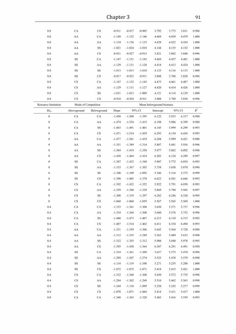
Chapter 3 91

0.8 CA CS -0.911 -0.917 -0.905 3.792 3.773 3.811 0.996

0.8 AA CA -1.149 -1.152 -1.146 4.469 4.459 4.479 1.000

0.8 AA AA -1.134 -1.136 -1.133 4.428 4.422 4.434 1.000

0.8 AA SS -1.021 -1.024 -1.018 4.144 4.135 4.152 1.000

0.8 AA CS -0.921 -0.927 -0.915 3.821 3.802 3.840 0.996

0.8 SS CA -1.147 -1.151 -1.143 4.469 4.457 4.481 1.000

0.8 SS AA -1.129 -1.131 -1.128 4.418 4.413 4.424 1.000

0.8 SS SS -1.013 -1.015 -1.010 4.125 4.116 4.133 1.000

0.8 SS CS -0.917 -0.923 -0.911 3.808 3.788 3.828 0.996

0.8 CS CA -1.147 -1.152 -1.143 4.473 4.461 4.487 1.000

0.8 CS AA -1.129 -1.131 -1.127 4.420 4.414 4.426 1.000

0.8 CS SS -1.011 -1.013 -1.009 4.121 4.114 4.129 1.000

0.8 CS CS -0.918 -0.924 -0.911 3.808 3.789 3.830 0.996

Resource limitation Mode of Competition Mean belowground biomass


0 CA CA -1.450 -1.508 -1.395 6.122 5.933 6.317 0.990

0 CA AA -1.474 -1.534 -1.415 6.198 5.986 6.399 0.988

0 CA SS -1.443 -1.491 -1.401 6.145 5.999 6.299 0.993

0 CA CS -1.471 -1.514 -1.429 6.293 6.154 6.436 0.993

0 AA CA -1.477 -1.541 -1.419 6.204 5.999 6.421 0.988

0 AA AA -1.351 -1.389 -1.314 5.807 5.681 5.936 0.996

0 AA SS -1.384 -1.419 -1.350 5.977 5.862 6.092 0.996

0 AA CS -1.438 -1.464 -1.414 6.203 6.124 6.289 0.997

0 SS CA -1.387 -1.432 -1.348 5.907 5.775 6.054 0.993

0 SS AA -1.333 -1.367 -1.303 5.758 5.658 5.870 0.996

0 SS SS -1.100 -1.109 -1.092 5.346 5.316 5.375 0.999

0 SS CS -1.390 -1.405 -1.378 6.623 6.581 6.666 0.993

0 CS CA -1.392 -1.432 -1.352 5.922 5.791 6.058 0.993

0 CS AA -1.359 -1.380 -1.339 5.869 5.790 5.945 0.997

0 CS SS -1.308 -1.319 -1.297 6.282 6.246 6.320 0.995

0 CS CS -1.060 -1.060 -1.059 5.567 5.565 5.569 1.000

0.4 CA CA -1.333 -1.361 -1.308 5.650 5.571 5.737 0.996

0.4 CA AA -1.334 -1.364 -1.308 5.660 5.576 5.752 0.996

0.4 CA SS -1.440 -1.473 -1.407 6.213 6.110 6.315 0.992

0.4 CA CS -1.487 -1.514 -1.462 6.411 6.334 6.494 0.993

0.4 AA CA -1.331 -1.359 -1.306 5.643 5.564 5.728 0.996

0.4 AA AA -1.312 -1.335 -1.289 5.563 5.489 5.633 0.998

0.4 AA SS -1.332 -1.355 -1.312 5.908 5.840 5.978 0.995

0.4 AA CS -1.395 -1.430 -1.364 6.387 6.291 6.491 0.958

0.4 SS CA -1.334 -1.361 -1.309 5.657 5.575 5.470 0.996

0.4 SS AA -1.289 -1.307 -1.274 5.525 5.478 5.579 0.998

0.4 SS SS -1.114 -1.119 -1.108 5.271 5.255 5.288 1.000

0.4 SS CS -1.072 -1.072 -1.071 5.418 5.415 5.421 1.000

0.4 CS CA -1.332 -1.360 -1.308 5.650 5.572 5.735 0.996

0.4 CS AA -1.284 -1.302 -1.269 5.510 5.462 5.563 0.998

0.4 CS SS -1.104 -1.110 -1.099 5.258 5.242 5.277 0.999

0.4 CS CS -1.070 -1.071 -1.069 5.414 5.411 5.417 1.000

0.8 CA CA -1.340 -1.365 -1.320 5.485 5.416 5.559 0.993

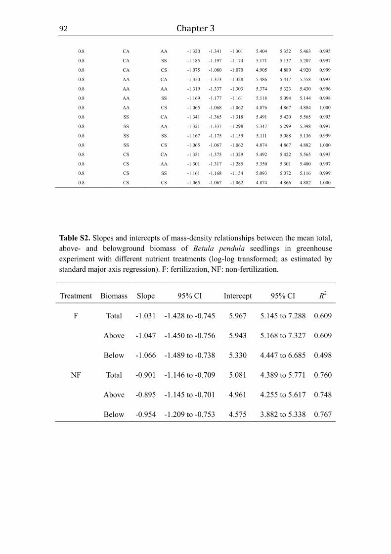
92 Chapter 3

Table S2. Slopes and intercepts of mass-density relationships between the mean total,

above- and belowground biomass of Betula pendula seedlings in greenhouse

experiment with different nutrient treatments (log-log transformed; as estimated by

standard major axis regression). F: fertilization, NF: non-fertilization.

0.8 CA AA -1.320 -1.341 -1.301 5.404 5.352 5.463 0.995

0.8 CA SS -1.185 -1.197 -1.174 5.171 5.137 5.207 0.997

0.8 CA CS -1.075 -1.080 -1.070 4.905 4.889 4.920 0.999

0.8 AA CA -1.350 -1.373 -1.328 5.486 5.417 5.558 0.993

0.8 AA AA -1.319 -1.337 -1.303 5.374 5.323 5.430 0.996

0.8 AA SS -1.169 -1.177 -1.161 5.118 5.094 5.144 0.998

0.8 AA CS -1.065 -1.068 -1.062 4.876 4.867 4.884 1.000

0.8 SS CA -1.341 -1.365 -1.318 5.491 5.420 5.565 0.993

0.8 SS AA -1.321 -1.337 -1.298 5.347 5.299 5.398 0.997

0.8 SS SS -1.167 -1.175 -1.159 5.111 5.088 5.136 0.999

0.8 SS CS -1.065 -1.067 -1.062 4.874 4.867 4.882 1.000

0.8 CS CA -1.351 -1.375 -1.329 5.492 5.422 5.565 0.993

0.8 CS AA -1.301 -1.317 -1.285 5.350 5.301 5.400 0.997

0.8 CS SS -1.161 -1.168 -1.154 5.093 5.072 5.116 0.999

0.8 CS CS -1.065 -1.067 -1.062 4.874 4.866 4.882 1.000

Treatment Biomass Slope 95% CI Intercept 95% CI R2

F Total -1.031 -1.428 to -0.745 5.967 5.145 to 7.288 0.609

Above -1.047 -1.450 to -0.756 5.943 5.168 to 7.327 0.609

Below -1.066 -1.489 to -0.738 5.330 4.447 to 6.685 0.498

NF Total -0.901 -1.146 to -0.709 5.081 4.389 to 5.771 0.760

Above -0.895 -1.145 to -0.701 4.961 4.255 to 5.617 0.748

Below -0.954 -1.209 to -0.753 4.575 3.882 to 5.338 0.767

Chapter 4

Exploring the interplay between modes of positive

and negative plant interactions *

Abstract

Facilitation (positive interaction) has received increasing attention in plant

ecology over the last decade. Just as for competition, distinguishing different

modes of facilitation (mutualistic, commensal or even antagonistic) may be

crucial. We therefore introduce the new concept of symmetric vs. asymmetric

facilitation and present a generic individual-based zone-of-influence model.

The model simultaneously implements different modes of both facilitation and

competition among individual plants via their overlapping zone of influence.

Because we consider facilitation modes as a continuum related to

environmental context, we integrated this concept with the stress gradient

hypothesis (SGH) by exploring differences in spatial pattern formation in

self-thinning plants along a stress gradient in our model. The interplay among

* A slightly revised version of this chapter has been published as Yue Lin1, 2

, Uta Berger1,

Volker Grimm2, 3

, and Qian-Ru Ji4 (2012) Differences between symmetric and asymmetric

facilitation matter: exploring the interplay between modes of positive and negative plant

interactions. Journal of Ecology 100: 1482–1491.

1 Institute of Forest Growth and Computer Science, Dresden University of Technology, P.O.

1117, 01735 Tharandt, Germany; 2 Helmholtz Centre for Environmental Research – UFZ,

Department of Ecological Modelling, 04318 Leipzig, Germany; 3 Institute for Biochemistry

and Biology, University of Potsdam, Maulbeerallee 2, 14469 Potsdam, Germany; 4

Institute of Hydrobiology, Dresden University of Technology, Zellescher Weg 40, 01062

Dresden, Germany

- 94 - Chapter 4

modes of interaction creates distinctly varied spatial patterns along stress

gradients. When competition was symmetric, symmetric facilitation (mutualism)

consistently led to plant aggregation along stress gradients. However,

asymmetric facilitation (commensalism) produces plant aggregation only under

more benign conditions but tends to intensify local competition and spatial

segregation when conditions are harsh. When competition was completely

asymmetric, different modes of facilitation contributed little to spatial

aggregation. Symmetric facilitation significantly increased survival at the

severe end of the stress gradient, which supports the claim of the SGH that

facilitation should have generally positive net effects on plants under high

stress levels. Asymmetric facilitation, however, was found to increase survival

only under intermediate stress conditions, which contradicts the current

predictions of the SGH. Our modelling study demonstrates that the interplay

between modes of facilitation and competition affects different aspects of plant

populations and communities, implying context-dependent outcomes and

consequences. The explicit consideration of the modes and mechanisms of

interactions (both facilitation and competition) and the nature of stress factors

will help to extend the framework of the SGH and foster research on facilitation

in plant ecology.

Keywords: asymmetry, competition, metabolic scaling theory, plant-plant

interaction, plant population and community dynamics, self-thinning, spatial

pattern, stress gradient hypothesis, symmetry

Chapter 4 - 95 -

4.1 Introduction

The role of positive interactions in driving population and community dynamics

has received significant attention and is now widely recognized in both

empirical and theoretical ecology (Bertness & Callaway 1994; Brooker et al.

2008; Bronstein 2009; Maestre et al. 2009; Fajardo & McIntire 2011; McIntire &

Fajardo 2011). In plant ecology, positive interactions are usually referred to as

facilitation, which has been defined as the beneficial effects of neighbours via

the amelioration of habitat (Bertness & Callaway 1994; Bronstein 2009); e.g.

via moderation of stress, enrichment of nutrients, or increased access to

nutrients. Facilitation has been shown particularly important when considering

the performance of plants under stressful environmental conditions. ‘Stress’ is

not a precise concept (Maestre et al. 2009), and can be biotic and abiotic

(Bronstein 2009). The best-understood examples of plant facilitation were

mostly carried out under abiotic stress conditions (Bronstein 2009). Moreover,

the characteristics of abiotic stress factors are also different and can be

resource-independent (e.g. wind, frost and salinity) or resource-dependent

(e.g. water, nutrient and light; Maestre et al. 2009).

The “stress gradient hypothesis” (SGH) proposes that competition and

facilitation may act simultaneously, but the relative importance of facilitation

and competition will vary inversely along gradients of abiotic stress (Bertness

& Callaway 1994). Under high stress conditions, facilitation should be

dominant over competition in affecting community structures (Bertness &

Callaway 1994; Brooker et al. 2008; Maestre et al. 2009). The SGH was

originally formulated at the interspecific level, but recent studies revealed that

SGH is also valid at the intraspecific level (Chu et al. 2008, 2009; Eränen &

Kozlov 2008; McIntire & Fajardo 2011). The interplay between facilitation and

competition can thus drive intraspecific population dynamics (Chu et al. 2008,

2009, 2010; Jia et al. 2011; McIntire & Fajardo 2011), community structure

- 96 - Chapter 4

(Gross 2008; Xiao et al. 2009), community diversity (Cavieres & Badano 2009),

and ecosystem functions (Callaway et al. 2002; Kikvidze et al. 2005); and can

even have evolutionary consequences (Bronstein 2009; McIntire & Fajardo

2011).

However, there are also studies which do not support SGH predictions, as

facilitative effects have not been detected under some extreme stress

conditions (Tielbörger & Kadmon 2000; Maestre et al. 2005, 2009). This

indicates that the conceptual framework underlying the SGH might need

further refinement (Maestre et al. 2009). Moreover, whereas numerous studies

have explored the consequences of different modes of competition, i.e.

symmetric versus asymmetric competition (Schwinning & Weiner 1998;

Weiner et al. 2001; Stoll & Bergius 2005; Berger et al. 2008), different modes

of facilitation have not yet been explored. Inconsistent definitions of facilitation

and the lack of differentiation between the impacts of plant-plant interactions

on beneficiary and benefactor individuals have recently been identified as

important gaps in current research (Brooker et al. 2008; Bronstein 2009;

Brooker & Callaway 2009; Pakeman et al. 2009). Refining and clarifying the

concept of facilitation is crucial for understanding how facilitation arises,

persists and evolves, and then could help extend the general SGH framework

and improve plant ecology research in general (Brooker et al. 2008; Bronstein

2009; Maestre et al. 2009).

According to different definitions, modes of facilitation can be mutualistic

(+/+) or commensal (+/0) amongst plants (Brooker et al. 2008; Bronstein 2009).

However, a more continuous approach to facilitative interactions might be

more accurate and useful, as has been the case for the corresponding

continuous approach to exploring competitive interactions (Schwinning &

Weiner 1998). We therefore suggest using a new concept of modes of

facilitation: any facilitation among plants, no matter whether inter- or

intra-specific, can be placed along a continuum ranging from completely

symmetric facilitation (interacting plants receive the same amount of benefit

Chapter 4 - 97 -

from each other, irrespective of their species or sizes) to completely

asymmetric facilitation (Vellend 2008; the beneficiary plant receives all benefits

but there are no positive effects on the benefactor; Table 4.1). Thus,

mutualistic cases are expected to be at the symmetric end of the facilitation

continuum, and commensal cases at the asymmetric end (Fig. S1).

Table 4.1 Definition and description of facilitation modes. The index q determines the

mode of facilitation among plants (see equation 5-5 and Appendix A).

Mode of

facilitation Effect and definition

Index

value

Expected prevalent

nature of stress factor

Complete

symmetry

All plants receive the same

amount of benefit from each

other, irrespective of their

species or sizes

q = 0

Symmetry:

temperature, moisture,

nutrient, salinity,

pollution, wind

desiccation, altitude etc.

Partial

symmetry

Benefit increases with

benefactor’s size, but less

than proportionally

0 < q < 1

Proportional

symmetry

Benefit is proportional to

benefactor’s size (equal gain

per unit size)

q = 1

Partial

asymmetry

Benefit increases with

benefactor’s size

super-linearly

q > 1 Asymmetry:

light, UV-radiation,

transpiration, tide, water,

nutrient fixation,

pollution, wind,

herbivory, etc.

Complete

asymmetry

The beneficiary plant

receives all benefits, with no

advantage to the benefactor

plants

q = ∞

This new conceptual model (with its terminology) has two main advantages:

it is analogous, and therefore directly comparable to the widely used and

important concept of symmetric and asymmetric competition (Schwinning &

- 98 - Chapter 4

Weiner 1998; Weiner et al. 2001; Stoll & Bergius 2005; Berger et al. 2008); it

also offers a quantitative and operational means of evaluating facilitative

impacts.

The analogy between different modes of competition and facilitation is

evident. In reality, competition and facilitation often interact: clusters of cohorts

facilitate each other against cold or wind desiccation (symmetric facilitation),

but they may also compete for nutrients and water (symmetric competition;

Fajardo & McIntire 2011). Adult nurse plants facilitate the growth and survival

of small plants of their own or other species (asymmetric facilitation), which

may lead to asymmetric light competition if the crown of an adult plant is very

dense or the small plants are not “stress-tolerant” (Reinhart et al. 2006;

Maestre et al. 2009). In general, modes of interaction depend on both the

ecological traits of the interacting plants and the nature of the stress factors

themselves (Maestre et al. 2009).

Competition usually leads to the spatial segregation of plants, implying that

distributions are more regular than aggregated (Stoll & Bergius 2005; Perry et

al. 2006). However, spatial aggregation is ubiquitous amongst varied plant

systems, especially in harsh environments (Bertness & Callaway 1994; Haase

2001; Perry et al. 2006). Because SGH predicts that facilitation should

dominate in such harsh environments, facilitation is believed to be an

important factor explaining plant aggregation in addition to other ecological

factors (e.g. topography, resource availability and dispersal) (Bertness &

Callaway 1994; Haase 2001; Perry et al. 2006). It has indeed been shown that

facilitation tends to maintain the aggregation of seedling cohorts and

established plants (Bertness & Callaway 1994; Fajardo & McIntire 2011; Jia et

al. 2011; McIntire & Fajardo 2011), but we do not yet know whether this is

generally true for different modes of facilitation and at different stress levels.

Consequently, we do not know how different modes of competition modify

the effects of facilitation on plants and structure their populations and

communities in different environmental contexts (Brooker et al. 2008). To

Chapter 4 - 99 -

address this issue, we implemented different modes of facilitation and

competition in a generic individual-based model based on the

zone-of-influence (ZOI) approach of Weiner et al. (2001). Plant growth and

density-dependent mortality are described according to a growth model as

deriving from “metabolic scaling theory” (MST; Brown et al. 2004; Savage et al.

2010) to provide mechanistic representation of plant response to stress. To

simplify, we restrict ourselves to intraspecific plant interactions. Specifically,

we addressed the following questions at both the plant population and

individual levels: (1) How does the interplay of different modes of competition

and facilitation change spatial pattern formation during self-thinning in

conspecific cohorts that initially have a random or aggregated distribution; and

(2) How do combinations of modes of competition and facilitation alter the

intensity of local plant interactions along a stress gradient?

4.2 Methods

4.2.1 The model

Metabolic scaling theory (MST) predicts quantitative relationships amongst

metabolic processes using empirical measurements and theoretical

assumptions (West et al. 2001; Enquist 2002; Enquist et al. 2009; Savage et al.

2010). We adopted these relationships as the basis of our individual growth

model for plants (see Chapter 2). The model is derived from an energy

conservation equation (Enquist & Niklas 2001; West et al. 2001; Hou et al.

2008) and takes into account respiration and three basic energy-demanding

processes: biomass maintenance, ion transport and biosynthesis (Lambers et

al. 2008). It provides a mechanistic and quantitative basis for linking the

energy used in metabolism of plants under abiotic stress to local interactions

and population dynamics. The growth model is:

- 100 - Chapter 4

dm/dt = am3/4 – bm = am3/4 [ 1 – ( m / M0)1/4 ] (4-1)

where m is total plant biomass, a and b are species-specific constants

(Chapter 2) determined by systematic variation of the in vivo metabolic rate of

different taxa (West et al. 2001), and M0 = (a/b)4 is the asymptotic maximum

size of a plant (calculated for dm/dt = 0). The term am3/4 in equation (4-1)

dominates during early plant growth and provides a good quantitative

description of plant growth (Enquist et al. 2009).

Because stress can be resource-independent or resource-dependent

(Maestre et al. 2009), we assume abiotic stress factors act in one or both of

two ways: by restricting the energy intake rate and burdening biomass

maintenance. This assumption provides a mechanistic basis for representing

the effects of stress on plant performance (Lambers et al. 2008). Accordingly,

the growth model with stress is:

dm/dt = (1 – S) am3/4 [ 1 – ( m / Ms)1/4 ] (4-2)

where S is a dimensionless efficiency factor that indicates the level of stress,

ranging from 0 (no stress) to 1 (extreme stress). Ms = (1–S)4M0 is the

maximum plant biomass achievable under stress.

Our individual-based model (IBM; Grimm & Railsback 2005) is described in

detail in the Supporting Information, following the ODD protocol (Overview,

Design concepts, Details) for describing individual-based models (Grimm et al.

2006; Grimm et al. 2010). In the following, we describe the model’s main

elements. In our IBM, a plant’s circular ZOI (Weiner et al. 2001), A, is the

physical space in which a plant acquires resources and represents the energy

and resources potentially available to the plant. This space is allometrically

related to plant biomass, m, as c0A = m3/4 (Enquist & Niklas 2001), where c0 is

a normalization constant. We represent plant interaction by calculating the

overlapping areas among the plants’ ZOIs (Weiner et al. 2001; Chu et al. 2008,

2009, 2010). Competition and facilitation under abiotic stress are incorporated

Chapter 4 - 101 -

by using dimensionless factors or indexes, fp and fq, respectively. With these

assumptions, equation (4-2) becomes:

dm/dt = fpfqcA[ 1 – ( m / M)1/4 ] (4-3)

where fp is the index of competition, fq refers to the abiotic stress (S) modified

by facilitation (see below), c = ac0 is the initial growth rate in units of biomass

per area and time, and M = (fpfq)4M0 is the maximum biomass achievable

under stress in the presence of competition and facilitation. Modes of

competition among plants can be defined along a continuum from completely

asymmetric competition (largest plants obtain all contested resources) to

completely symmetric competition (resources in areas of overlap are divided

equally among all overlapping individuals, irrespective of their relative sizes;

Schwinning & Weiner 1998). To represent the different modes of competition,

we define the index of competition, fp, as

,1

1

( ) /o

j

pn i i

p no o knk p

j jj

v mf A A A

v m

(4-4)

This index refers to the fraction of resources available in a given area to a plant

i after the loss of potential resources from areas overlapping neighbours with

biomass mj (Schwinning & Weiner 1998). Ano is the area with no overlap from

neighbours, and Ao,k denotes the no areas overlapping nj different neighbours.

The number of overlapping areas, no, can vary due to the position and number

of neighbours (see Appendix A). Parameter p indicates the mode of


(p approaching infinity). In this article we restrict ourselves to intraspecific

competition and facilitation, and assume, therefore, that the species-specific

weighting constants of competition vi and vj equal 1.

Similarly, we define the index of facilitation modifying abiotic stress, fq, as

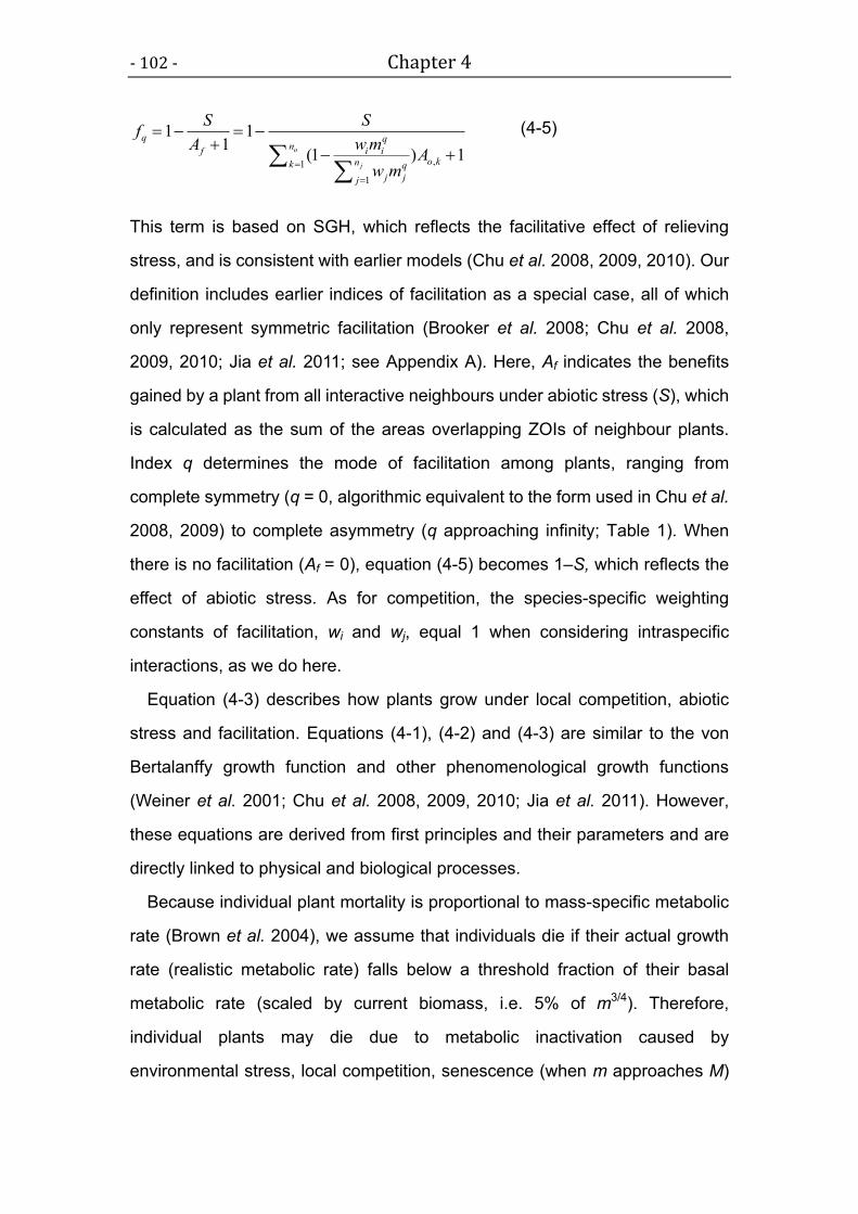
- 102 - Chapter 4

,1

1

1 11

(1 ) 1o

j

q qn

i ifo knk q

j jj

S Sf

wmAA

w m

(4-5)

This term is based on SGH, which reflects the facilitative effect of relieving

stress, and is consistent with earlier models (Chu et al. 2008, 2009, 2010). Our

definition includes earlier indices of facilitation as a special case, all of which

only represent symmetric facilitation (Brooker et al. 2008; Chu et al. 2008,

2009, 2010; Jia et al. 2011; see Appendix A). Here, Af indicates the benefits

gained by a plant from all interactive neighbours under abiotic stress (S), which

is calculated as the sum of the areas overlapping ZOIs of neighbour plants.

Index q determines the mode of facilitation among plants, ranging from

complete symmetry (q = 0, algorithmic equivalent to the form used in Chu et al.

2008, 2009) to complete asymmetry (q approaching infinity; Table 1). When

there is no facilitation (Af = 0), equation (4-5) becomes 1–S, which reflects the

effect of abiotic stress. As for competition, the species-specific weighting

constants of facilitation, wi and wj, equal 1 when considering intraspecific

interactions, as we do here.

Equation (4-3) describes how plants grow under local competition, abiotic

stress and facilitation. Equations (4-1), (4-2) and (4-3) are similar to the von

Bertalanffy growth function and other phenomenological growth functions

(Weiner et al. 2001; Chu et al. 2008, 2009, 2010; Jia et al. 2011). However,

these equations are derived from first principles and their parameters and are

directly linked to physical and biological processes.

Because individual plant mortality is proportional to mass-specific metabolic

rate (Brown et al. 2004), we assume that individuals die if their actual growth

rate (realistic metabolic rate) falls below a threshold fraction of their basal

metabolic rate (scaled by current biomass, i.e. 5% of m3/4). Therefore,

individual plants may die due to metabolic inactivation caused by

environmental stress, local competition, senescence (when m approaches M)

Chapter 4 - 103 -

or combinations thereof.

Our model was implemented in NetLogo 4.1.3 (Wilensky 1999). The source

code is available in the online supporting information of the publication

(http://onlinelibrary.wiley.com/doi/10.1111/j.1365-2745.2012.02019.x/suppinfo).

4.2.2 Scenarios and analysis

We investigated 2 modes of facilitation (q = 0: completely symmetric and q = ∞:

completely asymmetric) and 2 modes of competition (p = 0: completely

symmetric and p = ∞: completely asymmetric), at 3 stress levels (S = 0.1, 0.5

and 0.9). Two initial conditions were used: 300 initial plants distributed over

space either with aggregation or randomly (Fig. 4.1). For both aggregated and

random initial location scenarios, all simulations (42 scenarios in total) began

with exactly the same plant locations (i.e. using the same random number

seed), so that differences in results can be ascribed entirely to the interplay

among modes of competition and facilitation at different stress levels. (In

simulations not reported here, we used other initial densities, initial locations,

and interaction combinations to confirm that our general conclusions were not

artefacts of initial conditions.)

Ripley’s K function is widely used to analyse the spatial point pattern of

plants (Ripley 1981; Stoll & Bergius 2005; Perry et al. 2006). Here, we

employed the variance-stabilizing K function, the so-called Ripley’s L function,

to evaluate spatial pattern dynamics. The L function, L(r), characterizes the

point pattern at certain scales (r), with an expected value of zero under the null

hypothesis of complete spatial randomness (CSR). We carried out 499 Monte

Carlo simulations for each scenario to determine the 95% confidence

envelopes of the L function for CSR. Observed L(r) values out of the envelopes

indicate significant aggregation or regularity. Spatial point pattern data were

collected at 6 densities (300, 250, 200, 150, 100 and 50 plants) during the

self-thinning process. All statistical analyses were accomplished using R

2.11.1 (R Development Core Team, 2010).

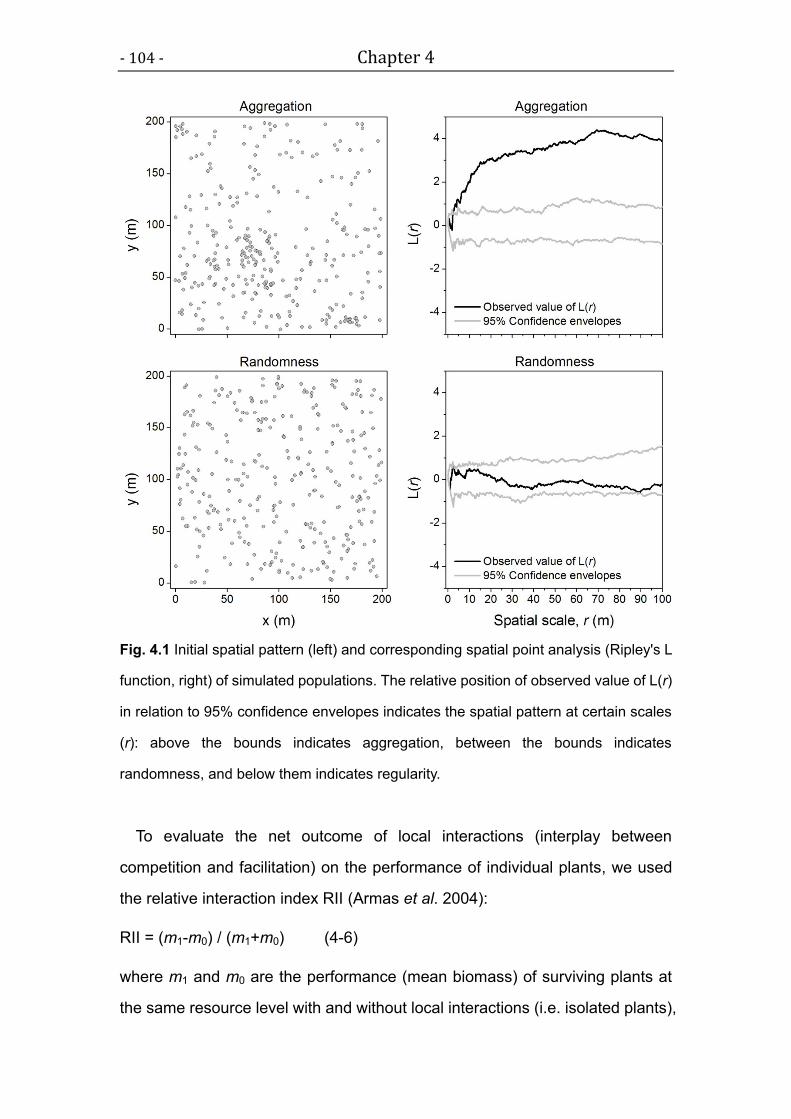
- 104 - Chapter 4

Fig. 4.1 Initial spatial pattern (left) and corresponding spatial point analysis (Ripley's L

function, right) of simulated populations. The relative position of observed value of L(r)

in relation to 95% confidence envelopes indicates the spatial pattern at certain scales

(r): above the bounds indicates aggregation, between the bounds indicates

randomness, and below them indicates regularity.

To evaluate the net outcome of local interactions (interplay between

competition and facilitation) on the performance of individual plants, we used

the relative interaction index RII (Armas et al. 2004):

RII = (m1-m0) / (m1+m0) (4-6)

where m1 and m0 are the performance (mean biomass) of surviving plants at

the same resource level with and without local interactions (i.e. isolated plants),

Chapter 4 - 105 -

respectively. Values of RII from -1 to 1 indicate the net outcome of interactions

as negative (from -1 to 0), neutral (equal to 0) and positive (from 0 to 1). To

estimate m0, we using equation (4-2) for plant growth in all scenarios.

4.3 Results

The interplay between competition and facilitation strongly influenced spatial

pattern formation in the plant population along the stress gradient. Different

modes of competition and facilitation also led to distinct spatial patterns. With

aggregated initial locations (Fig. 4.1), facilitation was vital for maintaining

aggregated patterns if competition was completely symmetric (CCS, p = 0) (Fig.

4.2). Without facilitation (NF), aggregation was maintained only until the

number of surviving plants decreased to 200 (Fig. 4.2a−c). With symmetric

facilitation (FCS, q = 0), plant aggregation patterns can be maintained (Fig.

4.2d−f) even at quite low density (100 plants), depending on the level of stress.

Aggregated patterns are particularly robust at high stress levels, which is

consistent with the predictions of SGH.

In contrast, with asymmetric facilitation (FCA, q = ∞), aggregating (Figs 4.2g

and 4.2h) can be maintained only at mild or intermediate stress levels (S = 0.1

and 0.5). Under harsh conditions (S = 0.9), aggregation disappears early in the

self-thinning process (Fig. 4.2i), a result that deviates from predictions of SGH.

However, modes of facilitation had little effect on maintaining aggregation

when competition was completely asymmetric (CCA, p = ∞; Fig. S2).

The importance of facilitation for creating aggregation became more obvious

when the initial pattern was random (Fig. 4.3). Under completely symmetric

competition without facilitation and under benign condition, there was some

slight spatial aggregation (values of L(r) were very close to the upper boundary

of the 95% confidence envelopes defining lack of aggregation) at very small

scales (Fig. 4.3a), but this aggregation instantly disappeared when stress

- 106 - Chapter 4

increased (Fig 4.3b and 4.3c). In contrast, more pronounced aggregation

patterns emerged in the presence of facilitation: symmetric facilitation

consistently forced aggregation under harsh conditions (Fig. 4.3d−f);

asymmetric facilitation led to aggregation only when stress was milder (Fig.

4.3g−i). Nevertheless, asymmetric competition can largely override the effects

of facilitation on spatial pattern formation at all stress levels, leading to

non-aggregative (even regular) spatial distributions (Fig. S3). This is in

agreement with empirical findings (Stoll & Bergius 2005).

Fig. 4.2 Spatial dynamics (black, aggregation; grey, randomness; white, regularity)

during self-thinning, with aggregated initial locations and completely symmetric

competition (CCS, p = 0) in the absence (NF) or presence of facilitation (FCS,

completely symmetric facilitation, q = 0; FCA, completely asymmetric facilitation, q = ∞)

at different levels of abiotic stress (S).

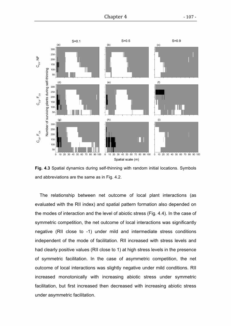
Chapter 4 - 107 -

Fig. 4.3 Spatial dynamics during self-thinning with random initial locations. Symbols

and abbreviations are the same as in Fig. 4.2.

The relationship between net outcome of local plant interactions (as

evaluated with the RII index) and spatial pattern formation also depended on

the modes of interaction and the level of abiotic stress (Fig. 4.4). In the case of

symmetric competition, the net outcome of local interactions was significantly

negative (RII close to -1) under mild and intermediate stress conditions

independent of the mode of facilitation. RII increased with stress levels and

had clearly positive values (RII close to 1) at high stress levels in the presence

of symmetric facilitation. In the case of asymmetric competition, the net

outcome of local interactions was slightly negative under mild conditions. RII

increased monotonically with increasing abiotic stress under symmetric

facilitation, but first increased then decreased with increasing abiotic stress

under asymmetric facilitation.

- 108 - Chapter 4

Fig. 4.4 Relative interaction intensity (RII) during self-thinning under different modes

of competition (CCS, completely symmetric competition, p = 0; CCA, completely

asymmetric competition, p = ∞) in the absence (NF) or presence of facilitation (FCS,


at different levels of abiotic stress (S), and with aggregated initial locations.

Facilitation sometimes resulted in spatial aggregation (Figs 4.2 and 4.3)

even though the net outcome (RII) of local interaction was negative. This

spatial patterning also depended on the mode of competition. Such results

indicate that even though facilitation was responsible for resulting plant

aggregation, the net outcome of local interaction was not always positive under

harsh conditions. In other words, modes of interaction can have different

effects on different population characteristics, i.e. here individual growth (RII)

and spatial pattern.

Chapter 4 - 109 -

Symmetric facilitation not only mitigated abiotic stress but also delayed the

onset of mortality in the case of symmetric competition, at all stress levels

(Duncan’s test, P < 0.05). Symmetric facilitation delayed the self-thinning

process, as indicated by the increased survival over time (Fig. 4.5).

Asymmetric facilitation had the same effect only at intermediate stress levels,

not at harsh conditions (Duncan’s test, P > 0.05). However, in the case of

asymmetric competition, the effects of facilitation were relatively weak.

Fig. 4.5 Temporal dynamics of density-dependent mortality under different modes of

competition (CCS, complete symmetric competition, p = 0; CCA, complete asymmetric

competition, p = ∞) in the absence (NF) or presence of facilitation (FCS, completely

symmetric facilitation, q = 0; FCA, completely asymmetric facilitation, q = ∞) at different

levels of abiotic stress (S), and for both initial location scenarios.

- 110 - Chapter 4

4.4 Discussion

We have introduced the new concept of modes of facilitation, i.e. symmetric

versus asymmetric facilitation, and have used an individual-based model to

explore how these facilitation modes affect plant populations differently.

Specifically, we explored how the interplay between different modes of

competition and facilitation changes spatial pattern formation during

self-thinning in populations that start with either random or aggregated

distributions, and how combinations of competition and facilitation modes alter

the intensity of local plant interactions along a stress gradient.

Our main finding was that the spatial aggregation of plants can be attributed

to different modes of facilitation if competition is symmetric rather than

asymmetric, whereas non-aggregative (regular) patterns indicate strong

asymmetric competition driving density-dependent mortality (Stoll & Bergius

2005). Facilitation by itself can play an important role in promoting plant

aggregation independent of other ecological factors ignored in our scenarios

(e.g. seed dispersal, recruitment, and environmental heterogeneity); moreover,

different modes of facilitation led to different spatial and temporal patterns.

In our simulations of harsh conditions, plants had highest biomass

accumulation and survival under the combination of symmetric competition

and facilitation. This result emerged from growing in association with

neighbours due to facilitation and the increased importance of facilitation at

higher stress levels as predicted by SGH. McIntire & Fajardo (2011) found that

spatial aggregation and symmetric interactions in Nothofagus pumilio are

essential for the species’ success under harsh conditions. Seedlings growing

in clustered cohorts facilitate each other and have higher survival rates than

isolated individuals under stress of wind desiccation. With seedlings growing in

clusters, natural grafts (physiological and physical merging of stem, branch or

root) occur in later growth stages, and multi–stemmed trees survive better than

single-stemmed trees. The mode of facilitation and competition among grafted

Chapter 4 - 111 -

plants is considered to be symmetric because the transport of resources and

assimilates is bidirectional (Silvertown & Charlesworth 2001; Lambers et al.

2008). The combination of symmetric facilitation and competition in these tree

clusters decreases the impact of stress and the onset of competition among

them (Fajardo & McIntire 2010; Tarroux & DesRochers 2011). Therefore,

mortality is lower within clusters and leads to aggregation, an outcome we also

found in our model.

Because we based our model of facilitation on SGH, a monotonic increase

in the importance of facilitation with increasing stress should be expected due

to the assumptions underlying equation (4-5). Surprisingly, this effect was

outweighed by asymmetric facilitation. Our study indicated that with symmetric

competition, asymmetric facilitation first promotes plant aggregation under mild

and intermediate stress conditions, but then brings about spatial

disaggregation at the more stressful end of the gradient (Fig. 4.2g−i).

Moreover, asymmetric facilitation was found to delay the self-thinning process

(indicated by increased survival over time) only under intermediate stress

conditions (Fig. 4.5). This is because under very stressful conditions, plants

are very sensitive to physical stress and local competition. Competition will

thus aggravate the mortality of those individuals that were disadvantaged by

asymmetric facilitation. Asymmetric facilitation can thus promote plant survival

and aggregation only if the environment is less harsh, as we observed in our

model.

Our results regarding asymmetric facilitation are consistent with recent

empirical findings that the SGH is not fully supported by observations (Maestre

et al. 2009). Reduced positive effects on plant survival have been observed in

arid areas at high stress levels (Tielbörger & Kadmon 2000; Maestre et al.

2005; Maestre et al. 2009). A switch from negative to positive and back to

negative effects on plant survival was found in a semi-arid steppe along a

gradient of decreasing rainfall (Maestre & Cortina 2004). Similarly, Tielbörger &

Kadmon (2000) found that the effect of desert shrubs on abundance and

- 112 - Chapter 4

reproductive success of understory annuals shifted from positive to neutral and

to negative with decreasing annual rainfall.

Our findings suggest a mechanism explaining such exceptions to the SGH’s

prediction of monotonic increasing net positive effect with stress: the nature of

abiotic stress factors is also important (Maestre et al. 2009). Abiotic stress

factors not only alter the mode of competition (Schwinning & Weiner 1998;

Berger et al. 2008), but also the mode of facilitation (Maestre et al. 2009). It is

therefore important to ask how symmetric and asymmetric facilitation are

interrelated with different kinds of stress factors. In the light of the new concept

presented here, it should be expected that if the effect of stress is

symmetrically mitigated by other individuals, symmetric facilitation should

usually be prevalent (detected via plant aggregation or positive RII in our

simulation). Using an individual-based model, Chu et al. (2009) found that

symmetric facilitation (mutualism) among plants can increase plant biomass

and size inequality in conspecific populations. Their results are consistent with

empirical findings for an annual species (Elymus nutans) in alpine meadows

(although they worked with clonal ramets, which probably confounded

physiological integration with positive interactions among individuals; Fajardo

& McIntire 2011). The mode of facilitation in their experiment was probably

symmetric because frost is the most important stress factor in their research

area (Chu et al. 2009): all individuals endure the same degree of low

temperature stress, which is not asymmetrically mitigated by other individuals.

In contrast, when the stress factor is “pre-mitigable” and/or directional (e.g.

higher ultraviolet radiation due to ozonosphere depletion or direct damage

caused by wind), facilitation should be more asymmetric (Fig. S1). For

example, in a conspecific plant population under strong ultraviolet radiation,

taller plants (benefactor) will suffer most from radiation stress but their crowns

can reduce stress in the understory microenvironment. As a result, smaller

plants (beneficiary) can receive disproportionately more benefit from their

neighbouring taller plants for maintenance and growth, and therefore survive

Chapter 4 - 113 -

longer. Asymmetric facilitation should thus reduce size inequality in plant

populations, which is in contrast to symmetric facilitation that can increase size

inequality (Chu et al. 2009). This effect of asymmetric facilitation is observed in

our model and consistent with empirical studies (Zhang et al. 2012). To the

best of our knowledge, effects of different modes of facilitation have not been

addressed systematically in empirical experiments yet, so we suggest this

topic for future research.

To answer our second research question about the effect of different

combinations of competition and facilitation on local interactions, we employed

the index RII to measure the direction and magnitude of local interactions

along a stress gradient. We found a monotonically increasing strength of

facilitation relative to competition for symmetric facilitation but not for

asymmetric facilitation. Negative interaction was dominant under mild and less

harsh conditions.

Our results indicate that even though facilitation can lead to plant

aggregation at the population level, the net outcome and intensity of local

interactions at the individual plant level is not necessarily positive. In particular,

we found that for some scenarios (e.g. CCS, FCA, S = 0.5), competition is the

dominant process when assessing plant growth (the net outcome is negative

as indicated by RII; Fig. 4.4), whereas the corresponding spatial aggregation

and greater survival probability indicate a dominance of facilitation (Figs 4.2,

4.3 and 4.5). In other words, the intensity of interaction (as the net outcome

between competition and facilitation) is insufficient to express the relative

importance of competition and facilitation on structuring plant systems

(Brooker et al. 2005). Furthermore, our findings imply that facilitation may be

more common than generally believed, but its important role in structuring

populations and communities can be hidden simply because it is hard to detect.

Thus, establishing whether competition or facilitation is the dominant process

in plant populations or communities can be difficult, because competition and

facilitation act simultaneously (Callaway 2007) but can affect different aspects

- 114 - Chapter 4

of plant populations or communities.

Nevertheless, the importance of facilitation has been clearly detected in arid,

alpine and arctic habitats, which are assumed highly sensitive to global change

(Callaway et al. 2002; Brooker et al. 2008). It is therefore crucial to better

understand both the mode of facilitation and nature of stress factors, because

the facilitative effect from key species is essential for system diversity and

stability in such conditions (Brooker et al. 2008; Vellend 2008). Although we

focused here on intraspecific interactions, our approach can easily be used to

analyse communities. Our conclusions may thus also be relevant for plant

communities.

To conclude, our study is the first to quantitatively define different modes of

facilitation, and it is also the first attempt to integrate different modes of

facilitation with different modes of competition into the SGH. We showed that

facilitation can have an important influence on population structure. Moreover,

different modes of facilitation and competition can affect different aspects of

plant populations and communities, implying context-dependent outcomes and

consequences. Explicit consideration of modes and mechanisms of interaction

(both facilitation and competition) and the nature of stress factors may help us

extend the SGH framework and foster research on facilitation in ecology

(Brooker et al. 2008; Maestre et al. 2009).

Acknowledgements

We thank Anne Fetsch, Jacob Weiner, Franka Huth, Rui-Chang Zhang and

Ming Yue for their kind help. We thank Steve Railsback for language editing.

We thank three anonymous reviewers and the handling editor for valuable

comments and suggestions. The first author was supported by Helmholtz

Impulse and Networking Fund through Helmholtz Interdisciplinary Graduate

School for Environmental Research (HIGRADE).

Chapter 4 - 115 -

References

Armas, C., Ordiales, R. & Pugnaire, F.I. (2004). Measuring plant interactions: a new

comparative index. Ecology, 85, 2682-2686.

Berger, U., Piou, C., Schiffers, K. & Grimm, V. (2008). Competition among plants:


research strategy. Perspectives in Plant Ecology, Evolution and Systematics, 9,

121-135.

Bertness, M.D. & Callaway, R. (1994). Positive interactions in communities. Trends in

Ecology & Evolution, 9, 191-193.

Bronstein, J.L. (2009). The evolution of facilitation and mutualism. Journal of Ecology, 97,

1160-1170.

Brooker, R.W. & Callaway, R.M. (2009). Facilitation in the conceptual melting pot. Journal

of Ecology, 97, 1117-1120.

Brooker, R., Kikvidze, Z., Pugnaire, F.I., Callaway, R.M., Choler, P., Lortie, C.J. &

Michalet, R. (2005) The importance of importance. Oikos, 109, 63-70.

Brooker, R.W., Maestre, F.T., Callaway, R.M., Lortie, C.L., Cavieres, L.A., Kunstler, G., et

al. (2008). Facilitation in plant communities: the past, the present, and the future.

Journal of Ecology, 96, 18-34.


metabolic theory of ecology. Ecology, 85, 1771-1789.

Callaway, R.M. (2007) Positive Interactions and Interdependence in Plant Communities.

Springer, Dordrecht.

Callaway, R.M., Brooker, R.W., Choler, P., Kikvidze, Z., Lortie, C.J., Michalet, R., et al.

(2002). Positive interactions among alpine plants increase with stress. Nature,

417, 844-848.

Cavieres, L.A. & Badano, E.I. (2009). Do facilitative interactions increase species richness

at the entire community level? Journal of Ecology, 97, 1181-1191.

Chu, C.J., Maestre, F.T., Xiao, S., Weiner, J., Wang, Y.S., Duan, Z.H., et al. (2008).

Balance between facilitation and resource competition determines

biomass–density relationships in plant populations. Ecology Letters, 11,

1189-1197.

Chu, C.J., Weiner, J., Maestre, F.T., Xiao, S., Wang, Y.S., Li, Q., et al. (2009). Positive

interactions can increase size inequality in plant populations. Journal of Ecology,

97, 1401-1407.

Chu, C.J., Weiner, J., Maestre, F.T., Wang, Y.S., Morris, C., Xiao, S., et al. (2010). Effects


self-thinning in simulated plant populations. Annals of Botany, 106, 647-652.

- 116 - Chapter 4

Enquist, B.J. (2002). Universal scaling in tree and vascular plant allometry: toward a


ecosystems. Tree Physiology, 22, 1045-1064.


communities. Nature, 410, 655-660.

Enquist, B.J., West, G.B. & Brown, J.H. (2009). Extensions and evaluations of a general

quantitative theory of forest structure and dynamics. Proceedings of the National

Academy of Sciences, 106, 7046.

Eränen, J.K. & Kozlov, M.V. (2008). Increasing intraspecific facilitation in exposed

environments: consistent results from mountain birch populations in two subarctic

stress gradients. Oikos, 117, 1569–1577.

Fajardo, A. & McIntire, E.J. (2010). Merged trees in second-growth, fire-origin forests in

Patagonia, Chile: positive spatial association patterns and their ecological

implications. American journal of botany, 97, 1424-1430.

Fajardo, A. & McIntire, E.J. (2011). Under strong niche overlap conspecifics do not

compete but help each other to survive: facilitation at the intraspecific level.


Graham, B.F. & Bormann, F.H. (1966). Natural root grafts. The Botanical Review, 32,

255-292.

Grimm, V., Berger, U., Bastiansen, F., Eliassen, S., Ginot, V., Giske, J., et al. (2006). A

standard protocol for describing individual-based and agent-based models.

Ecological modelling, 198, 115-126.


The ODD protocol: A review and first update. Ecological modelling, 221,

2760-2768.


University Press, Princeton and Oxford.

Haase, P. (2001). Can isotropy vs. anisotropy in the spatial association of plant species

reveal physical vs. biotic facilitation? Journal of Vegetation Science, 12, 127-136.

Hou, C., Zuo, W., Moses, M.E., Woodruff, W.H., Brown, J.H. & West, G.B. (2008). Energy

uptake and allocation during ontogeny. Science, 322, 736.

Jia, X., Dai, X.F., Shen, Z.X., Zhang, J.Y. & Wang, G.X. (2011). Facilitation can maintain

clustered spatial pattern of plant populations during density-dependent mortality:

insights from a zone-of-influence model. Oikos, 120, 472-480.

Kikvidze, Z., Pugnaire, F.I., Brooker, R.W., Choler, P., Lortie, C.J., Michalet, R., et al.

(2005). Linking patterns and processes in alpine plant communities: a global study.

Ecology, 86, 1395-1400.

Lambers, H., Chapin, F.S. & Pons, T.L. (2008). Plant physiological ecology. 2nd edition.

Springer Verlag, New York.

Chapter 4 - 117 -

Maestre, F.T., Callaway, R.M., Valladares, F. & Lortie, C.J. (2009). Refining the

stress-gradient hypothesis for competition and facilitation in plant communities.


Maestre, F.T. & Cortina, J. (2004) Do positive interactions increase with abiotic stress? A

test from a semi-arid steppe. Proceedings of the Royal Society of London, Series

B, 271, S331-S333.

Maestre, F.T., Valladares, F. & Reynolds, J.F. (2005). Is the change of plant–plant

interactions with abiotic stress predictable? A meta-analysis of field results in arid

environments. Journal of Ecology, 93, 748-757.

McIntire, E.J. & Fajardo, A. (2011). Facilitation within Species: A Possible Origin of

Group-Selected Superorganisms. The American Naturalist, 178, 88-97.

Pakeman, R.J., Pugnaire, F.I., Michalet, R., Lortie, C.J., Schiffers, K., Maestre, F.T., et al.

(2009). Is the cask of facilitation ready for bottling? A symposium on the

connectivity and future directions of positive plant interactions. Biology Letters, 5,

577-579.

Perry, G.L., Miller, B.P. & Enright, N.J. (2006). A comparison of methods for the statistical

analysis of spatial point patterns in plant ecology. Plant Ecology, 187, 59-82.

R Development Core Team (2010) R: a language and environment for statistical

computing. R Foundation for Statistical Computing, URL http://www.R-project.org.

Last accessed 17 February 2012.

Reinhart, K.O., Maestre, F.T. & Callaway, R.M. (2006) Facilitation and inhibition of

seedlings of an invasive tree (Acer platanoides) by different tree species in a

mountain ecosystem. Biological Invasions, 8, 231–240.

Ripley, B.D. (1981) Spatial Statistics. John Wiley and Sons, New York.

Savage, V.M., Bentley, L.P., Enquist, B.J., Sperry, J.S., Smith, D.D., Reich, P.B., et al.

(2010). Hydraulic trade-offs and space filling enable better predictions of vascular

structure and function in plants. Proceedings of the National Academy of Sciences,

107, 22722.


asymmetry in competition among plants. Oecologia, 113, 447-455.

Silvertown, J.W. & Charlesworth, D. (2001) Introduction to plant population biology.

Blackwell Publishing Limited, Oxford, UK.

Stoll, P. & Bergius, E. (2005). Pattern and process: competition causes regular spacing of

individuals within plant populations. Journal of Ecology, 93, 395-403.

Sthultz C.M, Gehring C.A, & Whitham T.G. 2007. Shifts from competition to facilitation

between a foundation tree and a pioneer shrub across spatial and temporal scales

in a semi-arid woodland. New Phytologist, 173, 135-145.

Tarroux, E. & DesRochers, A. (2011). Effect of natural root grafting on growth response of

jack pine (Pinus banksiana; Pinaceae). American Journal of botany, 98, 967-974.

http://www.sciencedirect.com/science?_ob=RedirectURL&_method=externObjLink&_locator=url&_issn=00029297&_origin=article&_zone=art_page&_plusSign=%2B&_targetURL=http%253A%252F%252Fwww.R-project.org

- 118 - Chapter 4

Tielbörger, K. & Kadmon, R. (2000). Temporal environmental variation tips the balance

between facilitation and interference in desert plants. Ecology, 81, 1544-1553.

Vellend, M. (2008). Effects of diversity on diversity: consequences of competition and

facilitation. Oikos, 117,1075-1085.

Weiner, J., Stoll, P., Muller-Landau, H. & Jasentuliyana, A. (2001). The effects of density,


populations. The American Naturalist, 158, 438-450.

West, G.B., Brown, J.H. & Enquist, B.J. (2001). A general model for ontogenetic growth.

Nature, 413, 628-631.

Wilensky, U. (1999). NetLogo. Center for Connected Learning and Computer-Based

Modeling, Northwestern University. Available at:

http://ccl.northwestern.edu/netlogo/. Last accessed 17 February 2012.

Zhang, R.C., Lin, Y., Yue, M., Li, Q., Zhang, X.F., Liu, X., Chi, H., Chai, Y.F. & Wang, M.

(2012) Effects of Ultraviolet-B Irradiance on Intraspecific Competition and

Facilitation of Plants: Self-Thinning, Size Inequality, and Phenotypic Plasticity.

PLoS ONE, 7, e50822.

Chapter 4 - 119 -


ODD protocol – model description of pi model with competition

and facilitation




Purpose

The aim of this model is to evaluate the multiple effects of the modes of

competition and facilitation under abiotic stress on regulating plant population

dynamics, specifically on spatial pattern formation induced by

density-dependent mortality. In particular, we test whether different modes of

facilitations at individual plant level can result in the spatial aggregation of the

population. The model does not represent specific species, but generic ones.

Entities, state variables, and scales


A1). Plants are characterized by the following state variables: initial growth rate,

initial biomass, maximum biomass (asymptotic biomass), current biomass and

their position, i.e. coordinates of the stem. Each individual plant has its own

circular zone-of-influence (ZOI). The ZOI stands for the physical space

occupied by a plant, and represents the energy and resources potentially

available to this plant, which is allometrically related to its body mass.

Neighbouring plants only compete for the resources when their ZOIs are

overlapping.



torus world with a size of 200 × 200 patches (Grimm & Railsback 2005). Each

patch represents 1 m2 or 1 cm2 for woody- and non-woody plants, respectively.

The state of each patch is characterized by its resource availability. We use a

homogeneous environment here as all patches have the same, and constant,

degree of abiotic stress. One time step in the model represents approximately

one year for woody plants and one day for non-woody plants.

- 120 - Chapter 4





(woody/non-woody)

Plants

c Initial growth rate 1 ± 0.1 [kg m-2 time step-1] /

[mg cm-2 time step-1]

m0 Initial body mass 2 ± 0.2 [kg] / [mg]

M0 Maximal biomass 2×106 ± 2×105 [kg] / [mg]

m Current biomass [kg] / [mg]

A Zone of influence [m-2] / [cm-2]

Patches

S Abiotic stress level [0, 1]

Initialization


Density Number of plants 300 [ha-1] / [m-2]

Random seed To generate random number 123456789

(Aggregation) Number of cohort 6 (50 individuals / cohort)

(Aggregation) Cluster scale (diameter) 50% of the world size

Process overview and scheduling


distributed in the world. The processes of local competition, facilitation, growth

and mortality of each plant are fulfilled within each time step. In each step,

individual plants first sense the environment qualities of patches within their

ZOIs, the area (radius) of an individual plant’s ZOI is determined by its current

biomass. When their ZOIs are overlapping, individuals compete and facilitate

within the overlapping area. Thus, the overlapping area reflecting resources is

divided according to the mode of competition. At the same time, under abiotic

stress in the presence of facilitation, the overlapping area reflecting the

ameliorated habitat by neighbours is also divided according to the mode of

facilitation. Considering the outcome of the interaction process, all individual

plants grow according to the growth function. Plants with growth rates falling

below a threshold die and are removed immediately. The state variables of the

Chapter 4 - 121 -

plants are synchronously updated within the subroutines, i.e. changes to state

variables are updated only after all individuals have been processed (Grimm &

Railsback 2005).

Design concepts



ZOI approach, with the effects of different modes of competition and facilitation

under abiotic stress.


relationship or self-thinning trajectories (i.e. size distribution and spatial

distribution, respectively), population size inequality and spatial pattern, are

emerged from local interactions among plants under abiotic stress of their

environment.

Interaction: Individual plants interact via competition for resources and

facilitation from neighbours in the overlapping area of their ZOIs.

Stochasticity: Initial growth rate, initial biomass, maximum biomass and

initial position of plants are randomly taken from the intervals given in Table 1.

This introduces a certain level of heterogeneity among individual

characteristics to take into account that real plants are never exactly identical.

Observation: Spatial point patterns of plants, population size, biomass of

each plant, and mean biomass of all living plants are the main observations.

Initialization

If the initial spatial pattern is aggregation, we randomly choose several patches

(determined by the number of cohorts) as centers and to transplant groups of

individual plants (initial density / number of cohorts) among the centers within a

certain cluster diameter. In the case of randomness, individual plants are

randomly distributed according to the chosen initial density. Resources and

abiotic stress are spatially and temporally constant. Each plant has an initial

biomass (m0), maximal biomass (M0) and initial growth rate (c) drawn from

truncated normal distributions with average and intervals given in Table A1.

Input



Submodels

Plant growth

- 122 - Chapter 4

In our individual-based model the plant’s ZOI stands for the physical space

occupied by a plant and represents the energy and resources potentially



constant. Accordingly, Eqn (4-1) can be rewritten as

dm/dt = cA [ 1 – ( m / M0)1/4 ] (A1)

and with abiotic stress, it becomes

dm/dt = (1 – S) cA [ 1 – ( m / Ms)1/4 ] (A2)

where c = ac0, is the initial growth rates in units of mass per area and time

interval. For simplicity, we choose c = 1 ± 0.1 in our model. In addition, we

simulate the model with different c values. As expected, the results from

different values were qualitatively similar (consist with our findings).

Competition and facilitation under abiotic stress

Competition and facilitation are incorporated by using dimensionless factors or

indexes, fp and fq respectively. With the above assumptions, equation (A2)

becomes:

dm/dt = fpfqcA[ 1 – ( m / M)1/4 ] (A3)

where M = (fpfq)4M0 is the maximum achievable biomass under stress with

competition and facilitation.

As for competition, the modes of resource-mediated competition among





different modes of competition explicitly, we describe the competitive index fp

as

,1

1

( ) /o

j

pn i i

p no o knk p

j jj

v mf A A A

v m

(A4)

This factor thus refers to the fraction of resources available in the area

which plant i could obtain after a loss of potential resources due to areas

overlapped by neighbours of sizes mj (Schwinning and Weiner 1998). Ano is

the area not overlapping with neighbours, Ao,k denotes the no areas

overlapping with nj different neighbours. Parameter p determines the mode of

Chapter 4 - 123 -

competition, ranging from complete symmetry (p=0) to complete asymmetry (p

approaching infinity; for details and examples see Figure A2). In this research,

we restrict ourselves to intraspecific facilitation and competition, and assume

therefore the species-specific weighting constant of competition vi and vj equal

1 here, as conspecific case.

Simultaneously, assuming the effect of facilitation is additive (Molofsky

2001; Molofsky & Bever 2002; Chu et al. 2008, 2009), we define the effect of

different modes of facilitation, fq, as

,1

1

1 11

(1 ) 1o

j

q qn

i ifo knk q

j jj

S Sf

wmAA

w m

(A5)

This factor is based on SGH, which reflects the facilitative effect of

relieving stress and is consist with other model (Chu et al. 2008, 2009, 2010;

Jia et al. 2011; for details and examples see Figure A2). To keep things simple,

we follow the assumption of Chu et al. (2008, 2009) that the ZOI, A, is the

same for competition and facilitation (they could be different). Where Af refers

to the benefit gained by plant from all interactive neighbours, and is calculated

as the sum of the areas (ZOIs) overlapped with neighbour plants. The index q

determines the mode of facilitation among plants, ranging from complete

symmetry (q = 0, algorithmic equivalent to the form used in Chu et al. 2008;

2009) to complete asymmetry (q approaching infinity; see Table 1 for the

complete form and definitions). Since we investigate the monopopulation here,

to simplify, we assume the species-specific weighting constant w equals 1 here

as the conspecific case, so the facilitation is size dependent. When there is no

facilitation (Af =0), equation (A5) becomes 1–S, which reflects the effect of

abiotic stress.

Figure A2. An example of calculating the interactive indexes (equations A4

and A5) with different modes of competition and facilitation by dividing plants’

- 124 - Chapter 4

ZOI (zone-of-influence). Three plants with sizes m1, m2 and m3 are interacting

in this example. For plant 1, its ZOI (A) was divided into four parts: Ano, the

area not overlapping with the other two plants; Ao,1, the area overlapping with

plant 2; Ao,2, the area overlapping with plants 2 and 3; Ao,3, the area

overlapping with plant 3.

Then the actual area that plant 1 can take from Ao,1 is

1 1,1 ,12

1 21

p p

o o p pp

jj

m mA A

m mm

For Ao,2,

1 1,2 ,23

1 2 31

p p

o o p p pp

jj

m mA A

m m mm

And for Ao,3,

1 1,3 ,32

1 31

p p

o o p pp

jj

m mA A

m mm

therefore, the competitive index for plant 1 is:

where 3/4

1 0/A m c . For plant 1, the benefit received from neighbours is

and the facilitative index for plant 1 under abiotic stress is:

In total, equation (A3) clearly shows how a plant’s growth rate is jointly

determined by abiotic stress, S, competition, fp, and facilitation fq. This also

implies that a plant’s final size is usually smaller than its asymptotic maximum

size (M0) during environmental stress and local competition, but can increase

by the beneficial effects of neighbour plants via the amelioration of habitat.

Mortality

An individual’s mortality rate is proportional to its mass-specific metabolism (as

current total metabolic rate divide by body mass; Brown et al. 2004). Based on

Chapter 4 - 125 -

this, we assume that individuals die if their actual growth rate (dm/dt, realistic

metabolic rate) falls below a threshold fraction of their basal metabolic rate

(allometrically scaled with body mass), i.e. 5% of m3/4. Therefore, individual

plants may die due to metabolic inactivation driven by abiotic stress,

competition, senescence (when m approaches M) or combinations thereof.

This provides a more realistic representation of relevant ecological process

than in previous models (Stoll et al. 2002; Chu et al. 2009, 2010; Jia et al.

2011).

References


metabolic theory of ecology. Ecology, 85, 1771-1789.

Chu, C.J., Maestre, F.T., Xiao, S., Weiner, J., Wang, Y.S., Duan, Z.H. et al. (2008).


biomass–density relationships in plant populations. Ecol. Lett., 11, 1189-1197.

Chu, C.J., Weiner, J., Maestre, FT, Xiao, S., Wang, Y.S., Li, Q., Yuan, J.L., Zhao, L.Q.,

Ren, Z.W. and Wang, G.(2009), Positive interactions can increase size inequality

in plant populations. J. Ecol., 97, 1401–1407

Chu, C.J., Weiner, J., Maestre, F.T., Wang, Y.S., Morris, C., Xiao, S. et al. (2010). Effects


self-thinning in simulated plant populations. Ann. Bot., 106, 647-652.

Enquist, B.J. (2002). Universal scaling in tree and vascular plant allometry: toward a


ecosystems. Tree Physiol., 22, 1045-1064.


communities. Nature, 410, 655-660.

Enquist, B.J., West, G.B. & Brown, J.H. (2009). Extensions and evaluations of a general

quantitative theory of forest structure and dynamics. Proc. Natl Acad. Sci. USA.,

106, 7046-7051.

Grimm, V., Berger, U., Bastiansen, F., Eliassen, S., Ginot, V., Giske, J. et al. (2006). A

standard protocol for describing individual-based and agent-based models. Ecol.

Model., 198, 115-126.


The ODD protocol: A review and first update. Ecol. Model., 221, 2760-2768.


University Press, Princeton and Oxford.

Hou, C., Zuo, W., Moses, M.E., Woodruff, W.H., Brown, J.H. & West, G.B. (2008). Energy

uptake and allocation during ontogeny. Science, 322, 736-739.

Jia, X., Dai, X.F., Shen, Z.X., Zhang, J.Y. & Wang, G.X. (2011) Facilitation can maintain


insights from a zone-of-influence model. Oikos, 120, 472-480.

Lambers, H., Chapin, F.S. & Pons, T.L. (2008). Plant physiological ecology. 2nd edition.

- 126 - Chapter 4

Springer Verlag, New York, pp. 134-143.

Maestre, F.T., Callaway, R.M., Valladares, F. & Lortie, C.J. (2009). Refining the

stress-gradient hypothesis for competition and facilitation in plant communities. J.

Ecol., 97, 199–205.

Molofsky, J. & Bever, J.D. (2002). A novel theory to explain species diversity in landscapes:

positive frequency dependence and habitat suitability. Proc. R. Soc. Lond., B, Biol.

Sci., 269, 2389–2393.

Molofsky, J., Bever, J.D. & Antonovics, J. (2001). Coexistence under positive frequency

dependence. Proc. R. Soc. Lond., B, Biol. Sci., 2001, 268–277.

Niklas, K.J. (2005). Modelling below-and above-ground biomass for non-woody and

woody plants. Ann. Bot., 95, 315-321.

Niklas, K.J. & Enquist, B.J. (2001). Invariant scaling relationships for interspecific plant

biomass production rates and body size. Proc. Natl Acad. Sci. USA., 98,

2922-2927.

Price, C.A., Enquist, B.J. & Savage, V.M. (2007). A general model for allometric

covariation in botanical form and function. Proc. Natl Acad. Sci. USA., 104,

13204-13209.

Sack, L., Maranon, T., Grubb, P.J., Enquist, B.J. & Niklas, K.J. (2002). Global allocation

rules for patterns of biomass partitioning. Science, 296, 1923a.


asymmetry in competition among plants. Oecologia, 113, 447-455.

Stoll, P., Weiner, J., Muller-Landau, H., Müller, E. & Hara, T. (2002). Size symmetry of

competition alters biomass–density relationships. Proc. R. Soc. Lond. B: Biol. Sci.,

269, 2191-2195.

Travis, J.M.J., Brooker, R.W., Clark, E.J. & Dytham, C. (2006). The distribution of positive

and negative species interactions across environmental gradients on a dual-lattice

model. J. Theor. Biol., 241, 896–902.

West, G.B., Brown, J.H. & Enquist, B.J. (1999). A general model for the structure and

allometry of plant vascular systems. Nature, 400, 664-667.

West, G.B., Brown, J.H. & Enquist, B.J. (2001). A general model for ontogenetic growth.

Nature, 413, 628-631.

West, G.B., Enquist, B.J. & Brown, J.H. (2009). A general quantitative theory of forest

structure and dynamics. Proc. Natl Acad. Sci., 106, 7040-7045.

Chapter 4 - 127 -

Fig. S1. Conceptual model of the occurrence of mutualism versus commensalism in a

continuum of symmetric versus asymmetric facilitation.

Fig. S2. Spatial dynamics (black, aggregation; grey, randomness; white, regularity)

during self-thinning with aggregated initial locations and completely asymmetric

competition (CCA, p = ∞) in the absence (NF) or presence of facilitation (FCS,


at different levels of abiotic stress (S).

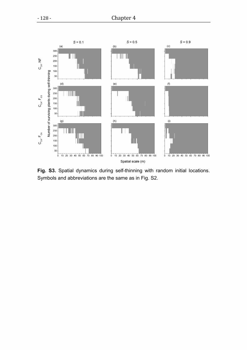
- 128 - Chapter 4

Fig. S3. Spatial dynamics during self-thinning with random initial locations.

Symbols and abbreviations are the same as in Fig. S2.

Chapter 5

Metabolic scaling theory predicts near ecological

equivalence in plants *

Abstract

Both niche and neutral theory aim to explain biodiversity patterns but seem

incompatible: whilst niche theory is based on the differences between species,

neutral models assume there are no such differences. Ecological equivalence

mediated by trade-offs however, is consistent with neutral theory whilst

allowing for ecological differences as suggested by niche theory. Here we show

with data from 375 plant species that metabolic scaling theory predicts such

trade-offs and thus supports ecological equivalence, at least as a near

approximation. This highlights a potentially important role for metabolic scaling

and points the way to a possible reconciliation between niche and neutral

theory.

Keywords: allometric scaling, neutral theory, ecological equivalence,

functional equivalence, demography, trade-offs, birth rate, death rate

* Manuscript in preparation

Yue Lin, Uta Berger, Volker Grimm, Qian-Ru Ji, James Rosindell, Jens Kattge, Helge

Bruelheide, and Richard Sibly

- 130 - Chapter 5

5.1 Introduction

Ecological difference among species (niche difference) is the conceptual basis

has been established since Darwin for explaining species coexistence and

diversity. By contrast, neutral theory (Hubbell 2001) provides models that

assume all species are ecologically identical. The idea received enormous

attention due to its accurate predictions despite its surprising simplicity, and

controversial assumption of ecological equivalence (Chave 2004; Rosindell et

al. 2012) which seems to be violated by many observable species-specific

characteristics.

One important aspect of neutral theory, however, has not yet been

sufficiently appreciated: ecological differences do not necessarily lead to

differences in net fitness (Chave 2004; Allouche & Kadmon 2009; Lin, Zhang,

& He 2009). Ecological equivalence regarding trade-offs between birth and

death rates among different species is still consistent with the neutral

assumption but allows for functional differences as suggested by niche theory

(Hubbell 2001; Chave 2004; Allouche & Kadmon 2009; Lin et al. 2009). It has

been shown in the simulation models that these birth-death trade-offs can be

incorporated into neutral theory without impairing its ability to predict

biodiversity patterns (Chave 2004; Lin et al. 2009; Rosindell et al. 2012).

Although predictions of neutral model have been tested extensively

(Hubbell 2001, 2005, 2006, 2008; Chave 2004; Allouche & Kadmon 2009; Lin

et al. 2009; Rosindell, Hubbell, & Etienne 2011), the cornerstone of neutral

theory which is the hypothesis of ecological equivalence has rarely been tested

(Hubbell 2008). Such ecological equivalence amongst individuals (species),

namely the demographic trade-offs, can be attributed to the intrinsic

explanations as neutral assumption assumed and/or the extrinsic explanations

as niche differences suggested. The intrinsic explanations are determined

essentially by the metabolism of organisms, whereas the extrinsic

Chapter 5 - 131 -

explanations are mainly related to external factors of environment such as

competition, resource, disease, predation or disaster (McCoy & Gillooly 2008).

In this study, we attempt to give a mechanistic, generic explanation for

these observed birth-death trade-offs, and thus provide a new and compelling

explanation for the success of neutral theory in a non-neutral world. To test our

predictions, we compiled data of demographic rates of 375 plant species which

include different functional groups and cover 11 orders of magnitude in plant

size ranging from mosses to trees.

The explanation we seek is provided by building on a base given by the

metabolic scaling theory (MST). This theory of ecology predicts quantitative

relationships between various functional traits of organisms and their body size

based on their metabolic rates (Brown et al. 2004; Price et al. 2010).

Extensions of MST yield that birth and death rates, b and d, are strongly

governed by the mass-specific metabolic rate (B), and thus should show the

body size (M) and temperature dependence (Brown et al. 2004; McCoy &

Gillooly 2008; Price et al. 2010) as:

b ∝ d ∝ B ∝ M -1/4e-E/kT (5-1)

where e-E/kT is the Boltzmann-Arrhenius factor which describes the exponential

increase in biochemical reaction rates with body temperature (Brown et al.

2004; Marbà et al. 2007; McCoy & Gillooly 2008; Price et al. 2010), E the

average activation energy of rate-limiting biochemical metabolic reactions (≈

0.32 eV for plants), k the Boltzmann’s constant (= 8.62×10－5 eV K－1), and T

the absolute temperature (Kelvin).

Although such scaling relationships have partly been statistically validated

before (Brown et al. 2004; Marbà, Duarte, & Agustí 2007; Price et al. 2010), so

far they were not linked to neutral theory. A reasonable estimation of overall

fitness (R0) can be measured as the ratio of birth rate over death rate which

- 132 - Chapter 5

gives the lifetime reproductive success or intrinsic rate of increase (Hubbell

2001; Chave 2004; Niklas 2007; Allouche & Kadmon 2009) leading to

R0 = b / d ∝ M -1/4 e-E/kT / M -1/4 e-E/kT ∝ M 0 (5-2)

Thus, fitness is predicted to be invariant with respect to body size, temperature,

as well as the metabolic rate across different functional groups of plant species.

It is almost self-explanatory that birth-death trade-offs is strongly governed by

the metabolic constrains of organisms, in other words, the intrinsic

mechanisms are expected to be the primary explanations. If this is true, the

overall fitness should be a constant among individuals and species, and the

ecological equivalence is to be expected as R0 = 1, which is also the parameter

setting of neutral models (Hubbell 2001; Chave 2004; Allouche & Kadmon

2009).

5.2 Materials and Methods

Temperature dependence of metabolism. Coexisting plant species in a

community can be assumed to experience the same temperature, so the

Boltzmann-Arrhenius factor can be omitted among species that coexisting in a

certain community. Moreover, the data set of birth and death rates analyzed in

this study also shows temperature independence (Student’s t-test, P = 0.43 and

P = 0.50 respectively), which is consistent with previous studies suggesting that

metabolic rates of plant are less temperature dependent than those of animals

(Marbà et al. 2007; Niklas 2007; Allouche & Kadmon 2009). Such findings

might also due to either statistical ‘‘noise’’ or the narrow band of temperature in

the data set (Marbà et al. 2007; Niklas 2007).

Data Compilation. Because the predictions of MST are base on a fractal-like

architecture of transporting network, so we compiled data on individual

average body masses, natural birth and death rates from a broad array of

higher plant species (excluding phytoplankton, algae, and macro-algae which

Chapter 5 - 133 -

do not have fractal-like architectures). Our data set includes mosses,

seaweeds, ferns, grasses, herbs, succulents, shrubs, lianas, mangroves as

well as other tree species. Each taxonomic group is represented by a diversity

of species and with plant body sizes span a very broad range (7.0×10-3 to

1.1×107g). All these data were primarily compiled from published data sets and

some are gathered from large census plots.

Measure of birth rate. We calculated the birth rates (b, in year -1) from initial

number of individuals (N0) and the number of new-born individuals (Nb) during

the time past between census interval (t, in year) as:

0 0ln ( ) ln ( )bN N Nb

t

(5-3)

Measure of death rate. The death rates (d, in year -1) are calculated as:

0ln ( ) ln ( )N Sd

t

(5-4)

where S indicates the number of survivors in the later census.

Estimate of tree mass. Tree mass (M, dry biomass in grams) that cannot

directly get was estimated from DBH (diameter at breast height in centimeters)

by using an allometric equation:

M = 78·DBH 2.5 (5-5)

this equation was fitted for a compilation of independent data set which

enclosing a very broad range of size for tree flora (Marbà et al. 2007).

Data Analysis. Because we are intend to answer different biological questions,

both Model I and II regressions are applied in our work by following the

suggestions about model selection (Smith 2009). To test the relationship

between body size (M) and the birth rates, death rates, and overall fitness (R0),

the allometric equations are fitted to log-transformed data by using ordinary

least squares regression (OLS, Model I regression). This is because we are

interested about how demographic rates change with plant body size. We use

- 134 - Chapter 5

the reduced major axis regression (RMA, Model II regression) for

log-transformed data fitting between birth and death rates. Because we

attempt to ascertain the actuality of ecological equivalence (b = d), meaning

that the bivariate relationship is symmetric and regardless of which variable is

dependent and which is independent.

5.3 Results and Discussion

Our analysis of data confirms that most plant populations examined here

are ecologically equivalent. Death rate, d, is proportional to the birth rate, b, as

d = 1.104 b 1.001 (Fig. 5.1 A). This does not differ statistically from the

equivalence in vital rates (b = d) assumed by neutral model. Furthermore,

observed distribution of the intrinsic rate of increase (R0 = b / d) is unimodal

with a mean of 1 (Fig. 5.1 B), implying a validity of nearly ecological

equivalence (Hubbell 2008).

In agreement with theoretical predictions, the data shows that species

balance high birth rates with high death rates according to mass-specific

metabolic rates and scale as -1/4 power of body mass (Fig. 5.2, A and B). The

overall fitness, R0, scales as M 0.006, and does not differ statistically from the

predicted mass invariance (M 0) (Fig. 5.2 C). Such results imply that ecological

equivalence as demographic trade-offs among different plant species are

largely constrained by intrinsic mechanisms of individual metabolic rate,

despite the fact that ecologically extrinsic factors exist in nature.

Nevertheless, the results also point to substantial variation (Fig. 5.1A) that

cannot be explained by metabolic constraints alone. Such variation might be

viewed as an indicator of non-neutral process among species from particular

communities, suggesting that both intrinsic and extrinsic constraints may

contribute to population and community dynamics. Therefore, it is more

relevant to test the relative contributions of intrinsic and extrinsic factors in

different populations and communities.

Chapter 5 - 135 -

Fig. 5.1 (A) The relationship between birth rates and death rates of plants (375

species). Red line shows the fitted reduced major axis regression (P < 0.0001, 95%

confidence intervals, exponent: 0.950 to 1.056, constant: 0.966 to 1.271). (B)

Distribution of the intrinsic rate of increase (overall fitness, calculated as the ratio

between birth rate and mortality rate, R0 = b / d) of plant species.

- 136 - Chapter 5

Fig. 5.2 (A) The relationship between plant body size and birth rates. Black

line shows the fitted ordinary least squares regression (OLS, Model I

regression; P < 0.0001, 95% confidence intervals, exponent: -0.315 to -0.232,

constant: 0.237 to 0.372). (B) The relationship between plant body size and

Chapter 5 - 137 -

death rates. Black line shows the fitted OLS regression (P < 0.0001, 95%

confidence intervals, exponent: -0.273 to -0.241, constant: 0.408 to 0.545). (C)

The relationship between plant body size and overall fitness (intrinsic rate of

increase, calculated as the ratio between birth rate and death rate, R0 = b / d).

Black line shows the fitted OLS regression (P < 0.707, 95% confidence

intervals, exponent: -0. 024 to 0.036, constant: 0.697 to 0.964).

Overall, our study indicates that neutrality as assumed by neutral theory

might be the consequence of scaling relationships which emerges from

constraints, trade-offs, and evolved characteristics of metabolism and

physiology. Meanwhile, MST also predicts different functional traits across

different functional groups of species (Brown et al. 2004; Price et al. 2010).

Thus, niches and neutrality are not excluding each other but might in fact have

the same mechanistic root. The current debate about whether niche or neutral

mechanisms structure natural communities might miss the point. The real

question should be when and why one of these factors dominates. Our

initiative work may provide some insights regarding the relative importance of

niche vs. neutral based process on community assembly and species

diversity.

References

Allouche, O. & Kadmon, R. (2009) A general framework for neutral models of

community dynamics. Ecology letters, 12, 1287–1297.

Brown, J.H., Gillooly, J.F., Allen, A.P., Savage, V.M. & West, G.B. (2004)

Toward a metabolic theory of ecology. Ecology, 85, 1771–1789.

Chave, J. (2004) Neutral theory and community ecology. Ecology Letters, 7,

241–253.

Hubbell, S.P. (2001) The Unified Neutral Theory of Biodiversity and

Biogeography. Princeton University Press.

Hubbell, S.P. (2005) Neutral theory in community ecology and the hypothesis

of functional equivalence. Functional ecology, 19, 166–172.

Hubbell, S.P. (2006) Neutral theory and the evolution of ecological

equivalence. Ecology, 87, 1387–1398.

- 138 - Chapter 5

Hubbell, S.P. (2008) Approaching ecological complexity from the perspective

of symmetric neutral theory. Tropical forest community ecology.

Wiley-Blackwell, Chichester, UK, 143–159.

Lin, K., Zhang, D.Y. & He, F. (2009) Demographic trade-offs in a neutral model

explain death-rate-abundance-rank relationship. Ecology, 90, 31–38.

Marbà, N., Duarte, C.M. & Agustí, S. (2007) Allometric scaling of plant life

history. Proceedings of the National Academy of Sciences, 104, 15777.

McCoy, M.W. & Gillooly, J.F. (2008) Predicting natural mortality rates of plants

and animals. Ecology letters, 11, 710–716.

Niklas, K.J. (2007) Sizing up life and death. Proceedings of the National

Academy of Sciences, 104, 15589.

Price, C.A., Gilooly, J.F., Allen, A.P., Weitz, J.S. & Niklas, K.J. (2010) The

metabolic theory of ecology: prospects and challenges for plant biology.

New Phytologist, 188, 696–710.

Rosindell, J., Hubbell, S.P. & Etienne, R.S. (2011) The Unified Neutral Theory

of Biodiversity and Biogeography at Age Ten. Trends in Ecology &

Evolution.

Rosindell, J., Hubbell, S.P., He, F., Harmon, L.J. & Etienne, R.S. (2012) The

case for ecological neutral theory. Trends in Ecology & Evolution, 27,

203–208.

Smith, R.J. (2009) Use and misuse of the reduced major axis for line‐fitting.

American journal of physical anthropology, 140, 476–486.

Chapter 6

General discussion

The general aim of my dissertation was to investigate the role of plant

interactions in driving population dynamics. Both theoretical and empirical

approaches were employed, such as individual-based models (IBMs) and

greenhouse experiment. All my studies are conducted on the basis of

metabolic scaling theory (MST, Brown et al. 2004, Price et al. 2010), because

the complex, spatially and temporally varying structures and dynamics of

ecological systems are considered to be largely consequences of biological

metabolism (Brown et al. 2004). On the other hand, MST didn’t consider the

important role of plant interactions and was found to be invalid in some

environmental conditions. Integrating the effects of plant interactions and

environmental conditions into MST may be essential for reconciling MST with

observed variations in nature. Such integration will improve the development

of theory, and will help us to understand the relationship between individual

level process and system level dynamics.

In the following, I will discuss what we in general learned from the work

presented in this thesis. First, I will discuss the pros and cons of mechanistic

and phenomenological models, in particular whether it paid to develop and use

an ontogenetic growth model. Then I will turn to plant competition and how

modelling it can be integrated with MST. Next, facilitation in combination with

competition will be discussed as a framework for exploring interactions of

plants with each other and their abiotic environment. The final two sections will

be devoted to synthesis: first, of plant competition, MST, and Neutral Theory,

and finally of the approach to addressing ecological questions used in this

thesis, Individual-Based Ecology.

- 140 - Chapter 6

Mechanistic models versus Phenomenological models

In the beginning of this dissertation, we deduced a mechanistic growth model

for plant. It is important that we use a mechanistic growth model derived from

MST rather than a phenomenological growth model, as usually has been done

so far in other plant IBMs (e.g., Weiner et al. 2001, Stoll et al. 2002, Stoll and

Bergius 2005, Chu et al. 2008, 2009, 2010, May et al. 2009). First, our

mechanistic growth model is based on the energy budget of the individuals

during growth which captures the key features of metabolic process of

organisms (West et al. 2001, Hou et al. 2008). Such mechanistic models

driven by ‘first principles’ are more flexible and are capable of capturing

adaptive responses of individuals to their environment than phenomenological

models, which are statistically fitted to existing data and forego any attempt in

explaining the underlying mechanisms (Hilborn and Mangel 1997, Grimm and

Railsback 2005, Martin et al. 2012). Second, the mechanistic models can be

easily extended to predict further patterns by deduction (e.g., the reproduction

biomass of individual plant, in Appendix of Chapter 1), whereas

phenomenological models are usually induced by patterns that were observed.

Mechanistic models are more likely to work correctly when extrapolating

beyond the current states than empirical models. Third, ecological or

mathematical artifacts are easier to be prevented if using mechanistic models

deduced from physical or physiological rules. For instance, in many IBMs plant

growth is assumed to be negatively and linearly related to resource

competition and environmental stress (Weiner et al. 2001, Stoll et al. 2002,

Stoll and Bergius 2005, Chu et al. 2008, 2009, 2010, May et al. 2009, Jia et al.

2011), with maximum body size kept constant. This phenomenological

assumption is both mathematical and ecological incorrect, because it implies

that plants can reach their optimal size regardless environmental conditions.

Fourth, in contrast to previous models used in plant IBMs (Wyszomirski 1983,

Wyszomirski et al. 1999, Weiner et al. 2001, May et al. 2009), our model is not

Chapter 6 - 141 -

only able to explain the observed variation in both root-shoot allocation

patterns, but also simultaneously describe the mass-density relationships (in

Chapter 3).

Yet, the merits of phenomenological/statistical models should not be

underestimated, especially when the aim is only to describe (or predict) rather

than to understand the mechanisms. Both the mechanistic models and

phenomenological models are useful, it is more relevant to ask how to choose

a model properly, in particular in IBMs. The POMIC (pattern-oriented modeling

information criterion, Piou et al. 2009) offers a rigorous statistical approach of

model selection which is in a context of POM (pattern-oriented modeling) and

is more efficient and specialized for IBMs. Nevertheless, in IBMs, with all other

things being equal, mechanistic models are arguably more powerful because

they can explain underlying processes driving observed patterns. Meanwhile,

the phenomenological models can also be used to stimulate and improve our

understandings on the mechanisms underlying observed patterns. A case in

point is how the ‘Kleiber’s law’ urge MST to come out (Brown et al. 2004).

Plant competition

In Chapter 2, we investigated the role of different modes of competition in

altering the prediction of MST on plant self-thinning trajectories. Our

spatially-explicit individual-based zone-of-influence (ZOI) model was

developed to investigate the hypothesis that MST may be compatible with the

observed variation in plant self-thinning trajectories if different modes of

competition and different resource availabilities are considered. Our one-layer

ZOI model supported our hypothesis that (i) size-symmetric competition (e.g.

belowground competition) will lead to significantly shallower self-thinning

trajectories than size-asymmetric competition as predicted by MST; and (ii)

individual-level metabolic processes can predict population-level patterns

when surviving plants are barely affected by local competition, which is more

likely to be in the case of asymmetric competition. In contrast to our findings,

- 142 - Chapter 6

some researchers proposed that asymmetric competition is more important to

explain the deviations predicted by MST (Coomes and Allen 2009, Coomes et

al. 2011). However, this debate again is due to a failure of distinguishing

between the ‘importance’ and ‘intensity’ of competition (Welden and Slauson

1986): we respect to the competitive effect on population level (mass-density

relationship) which is about the importance of competition, whereas they focus

on competitive response of single tree (individual tree growth) which is more

related to the intensity of competition.

In Chapter 3, we go further and add a bit more complexity by considering

the phenotypic plasticity and adaptive behaviour of plants in changing

environments. A two-layer ZOI model was developed which considers

allometric biomass allocation to shoots or roots and represents both above-

and belowground competition simultaneously via independent ZOIs. In

addition, we also performed greenhouse experiment to evaluate the model

predictions. Both our theoretical model and experiment demonstrated that:

plants are able to adjust their biomass allocation in response to environmental

factors, and such adaptive behaviours of individual plants, however, can alter

the relative importance of above- or belowground competition, thereby

affecting plant mass-density relationships at population level. Root competition,

which is assumed to be more symmetric, can strongly affect the growth of

surviving plants therefore alter the mass-density relationships. Invalid

predictions of MST are likely to occur where competition occurs belowground

(symmetric) rather than aboveground (asymmetric). Consequently, models or

theories which only consider aboveground part are not appropriate for the

cases where belowground processes predominate (Deng et al. 2006, Berger

et al. 2008). In addition to previous studies which do not consider the linkage

between above- and belowground competition, our study implies that adaptive

behaviours of plants such as allometry can modify ecological mechanisms and

subsequently the constraints set by MST. This has important implications for

many forests and eco-regions, e.g., for using allometry-based models to

Chapter 6 - 143 -

predict carbon storage and sequestration.

Plant competitions and metabolic scaling theory

Chapter 2 and 3 jointly showed that, MST, like principles from energetics and

biomechanics, sets limits on the behaviour of individuals and therefore of

populations and communities. In some ecological situations these limits will

dominate, and MST will predict higher-level behaviour. In many cases however,

other constraints will determine the patterns observed. Our most important

conclusion is that the behaviour of populations and communities may be

dominated by internal physiological mechanisms addressed by MST or by

ecological factors beyond the individual level, such as the type of resource

limitation and the mechanisms of competition among individuals. In the latter

cases MST will not be predictive, although nor will it be violated. The claim that

MST provides a ‘universal law’ for quantitatively linking the energetic

metabolism of individuals to ecological system dynamics is thus neither

completely right nor wrong: the real question is when and which factors

dominate in a given situation. However, our studies show that cross-level tests

are needed to explore and develop individual-level theories. Martin et al.

(2012), who used an individual-based population model of Daphnia based on

Dynamic Energy Budget theory (Kooijman 2009), arrived at the same

conclusion. Without doubts, the consideration of plant interactions is critical for

understanding variation in observed patterns.

Plant competition and facilitation

In Chapter 4, we introduced the new concept of modes of facilitation, i.e.

symmetric versus asymmetric facilitation, and developed an individual-based

model to explore how the interplay between different modes of competition and

facilitation changes spatial pattern formation in plant populations, and how

combinations of competition and facilitation modes alter the intensity of local

- 144 - Chapter 6

plant interactions along a stress gradient. Our study shows that facilitation by

itself can play an important role in promoting plant aggregation independent of

other ecological factors (e.g. seed dispersal, recruitment, and environmental

heterogeneity). Such finding identifies the origin of an important mechanism

underlying self-organization: the process of local facilitation among plants that

set against the background of overall control by environmental constrains.

Our results also indicate that the indices widely used to estimate intensity

of local interactions is too limited to represent the relative importance of

different modes of interactions in structuring plant system dynamics. Different

modes of facilitation and competition can affect different aspects of plant

populations and communities, leading to variously spatial and temporal

patterns, and implying context-dependent outcomes and consequences. For

instance, we find that the net outcome of local interactions among plants can

show a dominance of competition when using the index of relative interaction

intensity, in spite of the fact that local facilitation plays an important role in

structuring spatial aggregation. Although the intensity of interaction as the net

outcome is measurable, but the relative importance of competition and

facilitation in structuring system dynamics is much more complicated. To clarify

some debates in current ecological researches, it is necessary to distinguish

the differences between intensity and importance of different modes of

competition and facilitation, and to develop a comprehensive approach rather

than only use some indices. Moreover, a moderate mixture of positive and

negative interactions is demonstrated to stabilize population dynamics (Mougi

and Kondoh 2012). The diversity of species and interaction types may be the

essential element of biodiversity that maintains ecological communities, and

may hold the key to understanding population and community dynamics

(Grimm and Railsback 2005, Mougi and Kondoh 2012).

Towards a synthesis of metabolic scaling, niche, and neutral theory

In Chapter 5, we went from population level to community level and explored

Chapter 6 - 145 -

the possibility of combining the MST and unified neutral theory of biodiversity

(UNT, Hubbell 2001). Studies addressing UNT have largely focused on testing

the predictions of neutral models, whereas the fundamental assumption of

ecological equivalence has rarely been tested with empirical studies. Our

analysis of extensive data confirms that most plant populations examined are

nearly neutral in a sense of demographic trade-offs, which can mostly be

explained by a simple allometric scaling rule that based on MST. This

demographic equivalence regarding birth-death trade-offs between different

species and functional groups is consistent with the assumption of neutral

theory but allows functional differences between species (K. Lin et al. 2009).

Both niche and neutral mechanisms may be essential processes in community

assembly. In agreement with this, a new theoretical framework proposed four

basic processes in a community: natural selection (niche mechanisms),

ecological drift (neutral mechanisms), dispersal limitation and speciation. But

the relative importance of these four processes varies among communities

(Vellend 2008).

Current debate about whether niche or neutral mechanisms structure

natural communities apparently missing the point. Our initial study provides

some insights into this debate: the real question should be when and why one

of these factors dominates. Because UNT emphasizes neutral mechanisms

(ecological drift) as the main drivers of community assembly, for this reason

the demographic dynamics of all species in a certain community should be a

martingale. However, our results also show the variation of demographic

trade-offs that cannot be explained by metabolic constraints alone. Such

variation may be viewed as an indicator of non-neutral mechanisms (e.g.,

interactions and natural selection) among species in the communities, and the

goodness of fit (the coefficient of determination) may be viewed as the

contribution of neutral mechanisms. The empirical tests about the relative

importance of different mechanisms in natural communities are urgently

needed.

- 146 - Chapter 6

MST or similar bio-energetic theories (e.g., Dynamic energy budget

theory, Kooijman 2009) have the potential to unify existing biodiversity theories,

which are focused on abundances and species number, and link them to

questions regarding ecosystem functioning, e.g. productivity, plasticity, stability,

respiration, carbon flux etc. Such a synthesis of bio-energetic and

demographic theories is needed to better understand the relationship between

diversity and function of ecosystems and to unify future research in biodiversity

theory and management.

The Individual-Based Ecology

Ecology as a developing science is full of fresh ideas, but most of the

influential ideas still have not been mathematically well developed (Lawton

1999, Ghilarov 2003, Simberloff 2004, Grimm and Railsback 2005, Scheiner

and Willig 2008, 2011, Odenbaugh 2011a). Elaborate theories of ecology

which reflect ‘physics envy’ often omit the differences among organisms and

their traits, which I so-called ‘the assumption of spherical trees in a vacuum’.

However, since organisms are not just atoms such ‘physics envy’ theories are

of little use if we are going to understand the emergent properties of complex

systems such as population dynamics or community assembly out of

ecological traits, behaviours and interactions of individual organisms

(DeAngelis and Gross 1992, Breckling et al. 2005, Grimm and Railsback 2005).

The legendary ecologist MacArthur claimed “the best ecologists had blurry

vision so they could see the big patterns without being overly distracted by the

contradictory details” (Odenbaugh 2010, 2011b). Yet, an approach that can

‘zoom in and zoom out’ would be more appropriate if we are going to

understand the ecologically complex systems from individual levels (Grimm

and Railsback 2005). Accounting for omitted details often leads to more

refined theories. For instance, the van der Waals equation was derived as a

more precise version of the ideal gas law by incorporating the facts that

molecules have a nonzero volume and that they’re attracted to each other, for

http://en.wikipedia.org/wiki/Van_der_Waals_equation

Chapter 6 - 147 -

which Johannes van der Waals received the Nobel Prize for Physics in 1910

(Fox 2011). As in all such quests, it is important to keep in mind Einstein’s

dictum ‘seek simplicity, and distrust it’. Nevertheless, the main challenge in

ecology is to understand complexity and how it emerges from the adaptive

traits of individuals (Levin 2000, Grimm and Railsback 2005) which is the

major goal of individual-based ecology. The approaches of individual-based

and pattern-oriented modelling are promising to achieve the synthesis.

References




9:121–135.

Breckling, B., F. Müller, H. Reuter, F. Hölker, and O. Fränzle. 2005. Emergent properties

in individual-based ecological models—introducing case studies in an ecosystem

research context. Ecological Modelling 186:376–388.



Chu, C. J., F. T. Maestre, S. Xiao, J. Weiner, Y. S. Wang, Z. H. Duan, and G. Wang. 2008.


biomass–density relationships in plant populations. Ecology Letters

11:1189–1197.


and G. Wang. 2010. Effects of positive interactions, size symmetry of competition

and abiotic stress on self-thinning in simulated plant populations. Annals of Botany

106:647–652.

Chu, C. J., J. Weiner, F. T. Maestre, S. Xiao, Y. S. Wang, Q. Li, J. L. Yuan, L. Q. Zhao, Z.

W. Ren, and G. Wang. 2009. Positive interactions can increase size inequality in

plant populations. Journal of Ecology 97:1401–1407.

Coomes, D. A., and R. B. Allen. 2009. Testing the metabolic scaling theory of tree growth.





DeAngelis, D. L., and L. J. Gross. 1992. Individual-based models and approaches in

ecology: populations, communities and ecosystems. Chapman & Hall.

Deng, J. M., G. X. Wang, E. C. Morris, X. P. Wei, D. X. Li, B. Chen, C. M. Zhao, J. Liu, and

- 148 - Chapter 6

Y. Wang. 2006. Plant mass–density relationship along a moisture gradient in

north-west China. Journal of Ecology 94:953–958.

Fox, J. 2011. Why macroecology needs ‘microecology’: revisiting an Oikos classic.

http://oikosjournal.wordpress.com/2011/05/03/why-macroecology-needs-microec

ology-revisiting-an-oikos-classic/

Ghilarov, A. M. 2003. The changing place of theory in 20th century ecology: from

universal laws to array of methodologies. Oikos 92:357–362.

Grimm, V., and S. F. Railsback. 2005. Individual-Based Modeling and Ecology. Princeton

University Press.

Hilborn, R., and R. H. M. Mangel. 1997. The Ecological Detective: Confronting Models

with Data. Princeton University Press.

Hou, C., W. Zuo, M. E. Moses, W. H. Woodruff, J. H. Brown, and G. B. West. 2008.

Energy uptake and allocation during ontogeny. Science 322:736–739.

Hubbell, S. P. 2001. The unified neutral theory of biodiversity and biogeography.


Jia, X., X. F. Dai, Z. X. Shen, J. Y. Zhang, and G. X. Wang. 2011. Facilitation can maintain


insights from a zone-of-influence model. Oikos 120:472–480.

Kooijman, B. 2009. Dynamic Energy Budget Theory for Metabolic Organisation, 3rd

edition. Cambridge University Press.

Lawton, J. H. 1999. Are there general laws in ecology? Oikos:177–192.

Levin, S. A. 2000. Fragile Dominion: Complexity and the Commons. Basic Books.

Lin, K., D. Y. Zhang, and F. He. 2009. Demographic trade-offs in a neutral model explain

death-rate-abundance-rank relationship. Ecology 90:31–38.

Martin, B. T., E. I. Zimmer, V. Grimm, and T. Jager. 2012. Dynamic Energy Budget theory

meets individual-based modelling: a generic and accessible implementation.

Methods in Ecology and Evolution 3:445–449.

May, F., V. Grimm, and F. Jeltsch. 2009. Reversed effects of grazing on plant diversity:

the role of below‐ground competition and size symmetry. Oikos 118:1830–1843.

Mougi, A., and M. Kondoh. 2012. Diversity of Interaction Types and Ecological

Community Stability. Science 337:349–351.

Odenbaugh, J. 2010. Robert H. MacArthur.

Odenbaugh, J. 2011a. A General, Unifying Theory of Ecology? The Theory of Ecology:51.

Odenbaugh, J. 2011b. Philosophical themes in the work of Robert H. MacArthur.

Philosophy of Ecology 11:109.

Piou, C., U. Berger, and V. Grimm. (2009) Proposing an information criterion for

individual-based models developed in a pattern-oriented framework. Ecological

Modelling 220: 1957-1967.

Price, C. A., J. F. Gilooly, A. P. Allen, J. S. Weitz, and K. J. Niklas. 2010. The metabolic

theory of ecology: prospects and challenges for plant biology. New Phytologist

188:696–710.

Scheiner, S. M., and M. R. Willig. 2008. A general theory of ecology. Theoretical Ecology

1:21–28.

Scheiner, S. M., and M. R. Willig. 2011. The Theory of Ecology. University of Chicago

Chapter 6 - 149 -

Press.

Simberloff, D. 2004. Community ecology: Is it time to move on? The American Naturalist

163:787–799.

Stoll, P., and E. Bergius. 2005. Pattern and process: competition causes regular spacing

of individuals within plant populations. Journal of Ecology 93:395–403.


competition alters biomass–density relationships. Proceedings of the Royal

Society of London. Series B: Biological Sciences 269:2191–2195.

Vellend M (2010) Conceptual synthesis in community ecology. Quarterly Review of

Biology, 85, 183–206.

Weiner, J., P. Stoll, H. Muller‐Landau, and A. Jasentuliyana. 2001. The effects of density,


populations. The American Naturalist 158:438–450.

Welden, C. W., and W. L. Slauson. 1986. The intensity of competition versus its

importance: an overlooked distinction and some implications. Quarterly Review of

Biology:23–44.

West, G. B., J. H. Brown, and B. J. Enquist. 2001. A general model for ontogenetic growth.

Nature 413:628–631.

Wyszomirski, T. 1983. Simulation model of the growth of competing individuals of a plant

population. Ekologia Polska 31.

Wyszomirski, T., I. Wyszomirska, and I. Jarzyna. 1999. Simple mechanisms of size

distribution dynamics in crowded and uncrowded virtual monocultures. Ecological

Modelling 115:253–273.

Acknowledgments - 151 -

Acknowledgments

I have met many wonderful people during my PhD studies, I am really grateful to all

of them!

First of all, I would like to thank my advisor Uta Berger for all her generous help.

Uta gave me the freedom, trust and support to bring in my own ideas into this research

topic. But her opportune advices can always remind me the dreamer to put my feet on

the ground. I appreciate that she opened the door of mangroves to me and brought me

to an interesting field.

Many thanks go to my co-advisor Volker Grimm, who just has the magic to make

me be full of enthusiasm in my studies. When I was not convinced of my work, he

was the one who believed the merits of it even more than me. His ‘Scientific writing

course’ is the best course I have ever had.

I cannot express myself in words how thankful I am to Uta and Volker. I greatly

profited from their experience in science and life. The ‘facilitations’ I have received

from them are ‘completely asymmetric’. Without their supervision, I would never

have the opportunity to arrive the present thesis. As I said before, they are my mentors

forever.

There are a lot of people who helped me for some of my studies. I would like to thank

wholeheartedly: Franka Huth for her kind help on the greenhouse experiments, it

was so pleasure working with her. Jacob Weiner who is a co-author of one of my

manuscripts, his insightful comment not only improved the manuscript but also my

knowledge and experience of doing science. Juliane Vogt and Peter Frohberg, we

are “the best team in mangrove”. Prof. Dr. Steven Railsback for his help on my paper.

Prof. Dr. C. Edward Proffitt, Prof. Dr. Donna Devlin, and Prof. Dr. Candy Feller

for their kindly help during our research stays in Florida. Dr. Ulf Mehlig and Dr.

Moirah Menezes for their warmly help on our work in Brazil. Prof. Dr. James

Brown, Prof. Dr. Brian Enquist, Prof. Dr. Chen Hou, and Dr. Jian-Ming Deng for

their contributive suggests to my studies. Prof. Dr. Richard Sibly and Dr. James

Rosindell, Dr. Jens Kattge, and Prof. Dr. Helge Bruelheide for their kind help and

discussions on one of my manuscript. Dr. Stephen Wolfram, the conversation with

him inspired me to think the relationship between physics and ecology.

I wish to thank everyone in the Institut für Waldwachstum und Forstliche Informatik

for a friendly working atmosphere. Many thanks go to all my colleagues for their

moral support in daily PhD life, especially, Martin Schubert, Ronny Peters,

Andreas Tharang, Uwe Grüters, Mariana Vidal, Soledad Luna, Aor Pranchai,

Ursula Behr and Gisela Metzig. I am also grateful to my “doctoral bother”

Muhammad Ali Imron who is now in Indonesia.

- 152 - Acknowledgments

I would like also to thank Prof. Dr. Florian Jeltsch for accepting to evaluate my

dissertation, and Prof. Dr. Sven Wagner and Prof. Dr. Michael Müller to be on my

defense committee. I am also grateful for the help of Mrs. Bärbel Lommatzsch.

I could not have completed this doctoral dissertation without the support of

HIGRADE (Helmholtz Impulse and Networking Fund through Helmholtz

Interdisciplinary Graduate School for Environmental Research) fellowship. Many

thanks to my colleagues in UFZ.

At last, my love goes to my wife, Qian-Ru Ji for all her support and love during this

PhD thesis, for cheering me up and for her always so proud of me.

感谢我的母亲和父亲，没有你们的理解和支持，就没有我现在的一切。

感谢我的岳父和岳母，把茜茹交给了我，让我们可以自由自在的生活。

你们，是我们永远的港湾，我们取得的一切成绩也同样属于你们。

the role of different modes of interactions among

Documents