FEDERAL RESERVE BANK OF SAN FRANCISCO

WORKING PAPER SERIES

The Rise in Home Currency Issuance

Galina B. Hale Federal Reserve Bank of San Francisco

Peter Jones

University of California, Berkeley

Mark M. Spiegel Federal Reserve Bank of San Francisco

May 2016

The views in this paper are solely the responsibility of the authors and should not be interpreted as reflecting the views of the Federal Reserve Bank of San Francisco or the Board of Governors of the Federal Reserve System.

Working Paper 2014-19 http://www.frbsf.org/economic-research/publications/working-papers/wp2014-19.pdf

The Rise in Home Currency Issuance

Galina B. Hale

Federal Reserve Bank of San Francisco

Peter Jones

University of California, Berkeley

Mark M. Spiegel∗

Federal Reserve Bank of San Francisco

May 4, 2016

Abstract

Firms in countries outside global financial centers have traditionally found it difficult toplace bonds in international markets in their own currencies. Looking at a large sample ofprivate international bond issues in the last 20 years, however, we observe an increase in bondsdenominated in issuers’ home currencies. This trend appears to have accelerated notably afterthe global financial crisis. We present a model that illustrates how the global financial crisiscould have had a persistent impact on home currency bond issuance. The model shows thatfirms that issue for the first time in their home currencies during disruptive episodes, such as thecrisis, find their relative costs of issuance in home currencies remain lower after conditions returnto normal, partly due to the increased depth of the home currency debt market. Empirically, weshow that increases in home currency foreign bond issuance occurred predominantly in advancedeconomies with good fundamentals and especially in the aftermath of the crisis. Consistent withthe predictions of the model, financial firms – which are more homogeneous than their non-financial counterparts – in countries with stable inflation and low government debt increasedhome currency issuance by more. Our results point to the importance of both global financialmarket conditions and domestic economic policies in the share of home currency issuance.

JEL classification: F34, F36, F65, E52

Keywords: original sin, bond, debt, crisis, currency

∗We thank Philippe Bacchetta, Nicola Borri, Wenxin Du, Mathias Hoffman, Ken Kletzer, Catherine Mann, AndyRose, Asani Sarkar, Frank Warnock, and participants at the May 2014 SCIEA meeting, the West Coast Workshop onInternational Economics in Santa Clara in October 2014, the SNB Workshop on Foreign Currency lending in Europesince the Financial Crisis in Zurich in November 2014, Barcelona GSE forum in 2015, as well as seminar participantsat the BIS, University of Basel, and University of Zurich for useful comments. We are grateful to Javier Quintero forable research assistance. All errors are our own. The views in this paper are solely the responsibility of the authorsand should not be interpreted as reflecting the views of the Board of Governors of the Federal Reserve System or anyother person associated with the Federal Reserve System.

1 Introduction

It has become conventional wisdom that most countries do not borrow internationally in their own

currency, a phenomenon Eichengreen and Hausmann (1999) dubbed “original sin.”1 Indeed, Haus-

mann and Panizza (2003) point out that 97 percent of debt is issued in the five largest currencies,

henceforth “global currencies”—the U.S. Dollar, the euro, the British pound, the yen, and the Swiss

franc—yet borrowers in countries that are home to these currencies only account for 83 percent of

all debt issues. Theory predicts that foreign investors will demand premia on debt denominated

in high-risk countries’ currencies because of associated currency devaluation risk. As a result, bor-

rowers from high-risk countries often choose to denominate international debt in a global currency.

However, foreign currency debt may subject borrowers to currency mismatch, resulting in balance

sheet effects under exchange rate shocks.2 It may also limit the expansionary policy options of

monetary authorities, as countercyclical depreciation actions increase default risk for sovereign and

private borrowers facing currency mismatches (Eichengreen et al., 2007).

Academics and policymakers have long debated whether original sin results from poor poli-

cies and institutions or from structural features of international capital markets (Hausmann and

Panizza, 2011). More recently, developments have helped mitigate original sin through both chan-

nels. Inflation stabilization, often achieved through recently-adopted inflation targeting policies,

has garnered several previously-suspect countries new credibility, as regimes with formal inflation

targets have not only proven to be durable,3 but also have exhibited less exchange rate volatility,

and fewer sudden stops (Rose, 2007). Technological advancements may have also have decreased

the transaction and information costs of issuing in smaller currencies, reducing pressure for assets

to be issued only in global “reserve” currencies.

At the same time, the attractiveness of issuing in global currencies has changed as international

financial markets have evolved. Hale and Spiegel (2012) suggest that the advent of the European

1Eichengreen and Hausmann (1999) also use this term to describe the related fact that most countries also do notborrow domestically in their own currency at extended maturities. The focus of most subsequent work on originalsin and this paper, however, concerns the international dimension of original sin.

2For the importance of balance sheet effects see, for example, Krugman (1999), Schneider and Tornell (2004), andCalvo et al. (2008).

3Only Finland and Spain have abandoned inflation targets, doing so to join the European Monetary Union.

2

Monetary Union brought about a decline of the dollar’s dominance in international bond markets

by establishing a second global currency; of course, the introduction of the Euro mechanically

increased the number of countries able to borrow internationally in their own currency, but more

importantly, reduced the marked advantages of issuing in dollars. More recently, the global financial

crisis of 2008-09 disrupted the equilibrium in global financial centers, creating shortages of the U.S.

dollar, shaking the euro, and bringing global currency yields to the zero lower bound.

These changes appear to have mitigated the incidence of original sin. Hausmann and Panizza

(2011) update their earlier work (Hausmann and Panizza, 2003) with developing country data

through 2008, finding a small reduction in the incidence of original sin, limited to a few countries.

Burger and Warnock (2012) and Burger et al. (2015) document a strong trend of increasing U.S.

investment in local currency private and public bonds of emerging markets from 2001 to 2011. Du

and Schreger (2015a) demonstrate that between 2005 and 2011 the increase in foreign holding of

local currency debt issued by emerging markets was not unique to U.S. investors. They also show,

however, that this increase was primarily driven by increased foreign participation in domestic

sovereign bond markets. In fact, they do not observe a substantial increase in foreign holdings of

local currency corporate debt of emerging market borrowers.

We revisit the incidence of original sin using a large sample of private issues from non-global

currency countries, presenting evidence that countries’ abilities to borrow internationally in their

own currency has significantly increased over the last 20 years, and particularly since 2008. Fur-

thermore, we find that borrowers from many countries have, in fact, been “baptized” from original

sin, and now enjoy the ability to issue debt internationally in their home currencies. We present

a model to inform a discussion of the determinants of original sin and “baptism,” highlighting the

role of the global financial crisis. While most of the literature to date concentrates on half of the

borrower’s tradeoff— the costs and benefits of issuing in home currencies — we also emphasize the

other half—changes in the costs of issuing in a global currency—to explain the decline of original

sin.

Using micro-level data from Dealogic’s DCM Analytics (a.k.a. Bondware), we analyze the cur-

rency denomination of firms’ international bond issues by 10,037 firms from 32 non-global currency

3

countries between 1995 and 2013. We limit our empirical analysis to international bonds issued

by private sector firms for two reasons: First, as the 1998 Russian crisis showed, foreign participa-

tion in local bond markets can be very volatile, while issuance in international markets are more

stable; second, the data available on international bond issuance is much more consistent across

countries and therefore allows for a more systematic analysis. We did not find any robust patterns

in sovereign bond issuance and therefore excluded them from our analysis.4 We document a secular

decline in the use of the global currencies, and an increase in the share of deals denominated in

firms’ home currencies, which substantially accelerated after 2008.

We propose a simple model to better understand the circumstances under which firms’ propen-

sities to systematically issue a larger ratio of international debt in their home currencies might

increase, alleviating the incidence of origin sin. Our central assumptions are, first, that firms have

heterogeneous abilities to issue in their home currency, and pay country-specific premia on issues

denominated in their country’s currency relative to cost of issuing in a global currency; second,

that firms ”unseasoned” in issuing debt in their home currency pay an additional premium the

first time they issue debt in their home currency; third, that country-specific premia depend not

only upon conditions in the country itself, but also global economic conditions; and fourth, that

transaction costs associated with issuing in a given currency fall with increased overall issuance in

that currency. Specifically, we assume that country-specific premia decrease in the event of a global

crisis, due to either uncertainty in or shortages of global currencies (Caballero and Farhi, 2013), or

because of yield chasing by global investors. The model demonstrates how in the event of a crisis,

a temporary shock to the relative cost of home currency debt issuance may induce some firms to

issue in their home currency for the first time. This increase in the share of firms “seasoned” in

home currency issuance permanently reduces future home currency issuance costs. The result is

a post-crisis equilibrium that may differ from the pre-crisis equilibrium, even as macroeconomic

fundamentals return to normal. Because home currency premia are country-specific, the impact of

the crisis on firms’ susceptibility to original sin will differ across countries.

The model produces three testable hypotheses: first, non-global currency countries with bet-

4Currency composition of sovereign debt, including local debt purchased by foreign investors, is analyzed by Duand Schreger (2015b) and Alfaro and Kanczuk (2013).

4

ter fundamentals are more likely to have experienced an increase in the share of home currency

denominated foreign bond issues; second, countries with better fundamentals are also more likely

to increase the share of home currency issuance following the global financial crisis; third, these

effects are more pronounced the less dispersed are the firms’ idiosyncratic costs of issuing in home

currency. We then verify these hypotheses in the data.

First, we examine the characteristics of non-global currency countries that experienced a substan-

tive increase in the share of deals issued in home currency after the crisis. To do so, we estimate

country-industry cross-section regressions to investigate whether there was an increase in home

currency issuance from pre- to post- crisis years, controlling for industry fixed effects. We find

that advanced economies5 were more likely to experience an increase in home currency issuance.

Moreover, countries with low pre-crisis government debt and no history of recent inflation were also

more likely to increase their home currency deal share after the crisis.

Turning to issue-level panel regressions, we find no secular increase in the probability of home

currency issuance for borrowers from advanced economies, but instead a discrete increase in this

share following the global financial crisis. In contrast, for borrowers from emerging economies, we

observe a secular positive trend in the probability of home currency issuance that is uninterrupted

by the crisis and is not explained by changes in macroeconomic fundamentals.

For advanced economies, we also find that recent episodes of high inflation and high ratios

of government debt to GDP are jointly associated with lower probabilities of issuing in home

currencies, supporting the view that original sin results, at least in part, from poor policies.6

However, macroeconomic variables don’t seem to affect the probability of home currency issuance

for borrowers from emerging economies. We interpret this finding as suggesting that fundamentals

in emerging markets are too poor on average for those nations to increase their firms’ home currency

borrowing prospects through improved national policies.7

In terms of issue-specific variables, the results corroborate our model in at least three important

5We heretofore use the term ”advanced economies” to identify non-global-currency industrial countries.6These results are consistent with the results from a cross-country analysis of total, international and domestic,

local currency debt as of 2001 in Burger and Warnock (2006).7McCauley et al. (2015) show that in recent years emerging markets dollar borrowing was on the rise.

5

ways: (i) firms in industries with larger export shares are less likely to issue in home currency;

(ii) larger issues are less likely to be denominated in home currencies; and (iii) firms that have

previously issued in their home currency—which we refer to as being “seasoned” in home currency

issuance—are more likely to do so again.8

Our firm-level data set allows us to distinguish between financial and non-financial borrowers.

The model predicts that the more similar is the group of borrowers, the easier it is for them

to transition to home currency issuance. While financial firms are a rather homogeneous group,

the non-financial firms in our sample come from a large variety of industries. We would therefore

expect non-financial firms to be more diverse in terms of their propensity to issue in home currency.

Consistent with this prediction, we find that the increase in home currency issuance by advanced

economies in the aftermath of the crisis was entirely driven by financial firms. Moreover, the

significant sensitivity to macros variables, such as inflation history and debt-to-GDP ratio is also

only observed among financial firms.

Thus, the data show that improvement in macroeconomic fundamentals in advanced economies

helped their financial firms increase issuance in home currency. At the same time, the global

financial crisis brought about a temporary increase in the cost of borrowing in global currencies that

had persistent effects. Moreover, countries with better fundamentals prior to the crisis experienced

a larger increase in the share of home currency bond issuance afterwards. These results highlight

the interplay between domestic policies and features of international capital markets in explaining

the incidence of original sin.

The paper proceeds as follows. In section 2 we describe our data and present trends in the data

that motivate our analysis. In section 3 we present our model and its empirical application. Section

4 brings model prediction to the data. Section 5 concludes.

8Introducing a time trend in combination with firm fixed effects removes this effect.

6

2 Data Description

2.1 Data sources

Our empirical analysis is based on micro-level data from Dealogic’s DCM Analytics (a.k.a. Bond-

ware), which covers most new issues on the international bond market (Hale and Spiegel, 2012).

We limit our analysis to issues placed by private companies in foreign markets—those explicitly

marketed to foreign investors and labeled by Dealogic as “international issues.”9 Dealogic’s deal-

level data provide the name and nationality of the issuer,10 the deal amount, and currency. With

this information we classify deals as denominated either in home or foreign currency, and borrowers

as either seasoned or unseasoned in home, and separately in foreign, currency issuance.

In total, our sample contains 16,584 international bond issues by 2,147 firms from 30 countries

between 1995 and 2013.11 Excluded from this sample are the global currency countries—countries

whose currencies have traditionally dominated international trade invoicing and asset issuance

(Eichengreen et al., 2007): the U.S., the U.K, Japan, Switzerland, and all euro area countries.12

We also exclude financial centers, most notably Hong Kong and Singapore. We split the sample

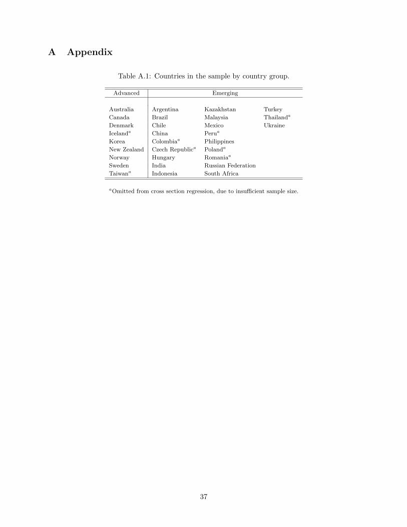
into borrowers from 9 advanced and 21 emerging economies, which are listed in Appendix Table

A.1. Appendix Table A.2 shows the number of deals and amounts borrowed by each group for each

year in our sample.

There are two primary weaknesses in our bond issuance data. First, the data only provide limited

issuer information and do not include firm identifiers that could be matched to other sources.

Consequently, we cannot include firm-level controls beyond issue size and bond issuance history.

Second, coverage of bonds issued in domestic markets is uneven across countries, which precludes

us from controlling for domestic issuance.13

9Some of these bonds may have explicit restrictions that forbid their trading in domestic markets.10We use “issuer nationality of operations” to identify deal nationality. This implies that bonds issued through

offshore financial centers do not get assigned the nationality of the offshore center, but rather the country of residenceof the issuer.

11We limit the sample to countries with at least 19 issues during the sample period (one per year on average), aminimum threshold for meaningful analysis.

12For the discussion of the currency composition of eurozone debt, see Bacchetta and Merrouche (2015).13For an analysis of domestic market bond issuance that uses alternative data sources, see Du and Schreger (2015a).

7

We match this bond-level data with country-level data from two sources: Gross government

debt and inflation data come from the IMF’s World Economic Outlook database. Exchange rate

data come from the IMF’s International Financial Statistics (IFS) database. Appendix Table A.3

presents summary statistics for variables used in our analysis.

DCM Analytics does not allow us to identify whether the issuer is an exporter or not, but we proxy

for firm export shares using country-industry-year export shares in total production. We construct

this measure in three steps. Country-industry export data with SITC descriptions come from the

United Nations Conference on Trade and Development. Using these descriptions we assign 2-digit

SITC codes to the data. Industrial production data at the 2-digit ISIC code level come from the

United Nations Industrial Development Organization. Next, we create a correspondence between

2-digit ISIC codes and 2-digit SITC codes to merge the export data with the industrial production

data. Finally, using 4-digit SIC descriptions included in the DCM Analytics data for each issuer, we

create a correspondence between 2-digit SIC codes and 2-digit ISIC codes to merge the (industry

level) ratio of exports to industrial production for each borrower.

2.2 Trends in home currency issuance across countries and over time

To motivate our discussion, we first document global trends and cross-country comparisons in the

data. In Figure 1, we examine the prevalence of global currencies across three major time periods

in our sample: pre-euro (1995-1998), euro pre-crisis (1999-2007), and post-crisis (2010-2013).14

Although not a global currency, we separate bond issues in the Hong Kong dollar whose dynamics

are likely driven by developments in China. In the pre-euro period the top five global currencies

dominate international debt issuance.15

The introduction of the euro prompts a substantial increase in the share of debt issued in the

euro at the expense of the yen, the U.S. dollar and the Swiss franc, as discussed in Hale and Spiegel

(2012) as well as an increase in British pound issuance. After the crisis, euro-denominated issuance

declines, reflecting concerns over the sovereign debt crisis in the euro area. A decrease in the

14We omit 2008-2009 to avoid potential oddities in the data that could be driven by crisis-specific circumstances.15For the dynamics of euro-denominated bond issuance, see the ECB July 2014 publication “The international role

of the euro,” pages 54-79.

8

share denominated in yen, British pound, Hong Kong dollar, and Swiss franc accompany the euro’s

decline. More striking is the substantial increase in the share denominated in “Other” currencies,

driven by large increases in the use of the Australian dollar (AUD), the Norwegian Krone (NOK),

and the Swedish Krona (SEK).

One potential source of this observed increase in non-global currency issuance could be that firms

in countries home to those currencies began issuing in their own currencies. Figure 2 shows for-

eign and home currency bond issuance by firms in advanced, and separately, by firms in emerging

economies. The top panel shows total debt in real US dollars; the bottom panel shows the num-

ber of deals. For both advanced and emerging economies, issuance in home currencies increased

throughout the sample, but particularly after the crisis. This increase is more pronounced for the

number of deals, rather than volume, implying that small deals are more likely to be denominated

in home currency than large ones.16

In Figure 3 we separate new issuers in the international bond market from those that previously

issued in foreign currency (seasoned in foreign currency), and those that previously issued in home

currency (seasoned in home currency), and show the prevalence of home currency issuance for each

type of borrower over time. Prior to 2000, firms in advanced economies that were seasoned in

home currency were much more likely to issue in their home currency again than firms that entered

international bond markets for the first time and firms that previously issued in foreign currencies.

Home currency issuance was much less common in emerging economies over the same period. An

increase in the ratio of firms issuing in home currency after the crisis is apparent for advanced

economies and noisily so for emerging economies.

Finally, in Figure 4 we show the change in the share of international bonds denominated in

home currency before and after the crisis (between 2002-2006 and 2010-2013). While some coun-

tries experienced small declines in the share of home currency issues,17 most countries, advanced

and emerging alike, experienced increases, with Australia, Canada, China, Norway, and Sweden

experiencing the most substantial hikes.

16Note also the drop of issuance in 2008, especially by emerging economies.17The exception is Hungary, with a 15 percentage point decline in its share of home currency issuance, due to the

severe balance of payments crisis it experienced as a result of the global financial crisis.

9

3 Determinants of transition to home currency issuance: model

What explains the above trends, and, in particular, the discrete increase in home currency issuance

following the global financial crisis? To shed light on this, we construct a model of an individual

firm’s choice between issuing a bond in their own home currency, or a global currency. The model

builds upon a similar set of assumptions as Hale and Spiegel (2012), but incorporates dynamics

that allow for an increased role of country fundamentals.

Our model characterizes the determinants of an individual debt issuer’s choice of currency de-

nomination, illuminating the circumstances under which firms might choose to issue a larger portion

of debt in their home currency.

We frame the model in terms of a representative firm from an economy which is atomistic in

terms of world financial conditions. There are 3 periods, t = 0, 1 and 2. Each firm issues one dollar

in one-period debt in periods 0 and 1 to finance an investment. The firm must decide whether

to issue in their home currency, h, or a foreign “hard” currency, f . Each firm, i, enters period 0

exogenously designated as either seasoned or unseasoned in issuing in their home currency, as a

result of past behavior which we do not model. Investments pay a fixed return Y in periods 1 and

2; any profits earned are immediately paid out as dividends.18

There are 2 ε̄ atomistic firms in the country. Firms therefore issue a total volume of 2 ε̄ in debt

each period. Firm income is invariant with respect to their financing choice, so decisions are solely

based on minimizing financing costs, with our analysis focusing on the currency denomination

decision.

We assume that four factors influence a firm’s choice of currency:

1. There exist economies of scale in total issuance in the home currency. Let Vt represent the

total volume of issues in the home currency at time t.

2. Firms differ in their ability to issue in the foreign currency. We model this by assuming that

in each period each firm receives an idiosyncratic shock, ε, which measures its disadvantage

in issuing in the foreign currency. We assume that these shocks are i.i.d., and distributed on

18In the same period that profits are earned.

10

support [−ε, ε] with mean 0 and density f(ε). These shocks could proxy for the denominations

of firms’ export revenues, foreign currency stock trading, or relative hedging ability.

3. Firms unseasoned in issuing in their home currency pay a premium, u, the first time they

issue in their home currency. While this assumption is not necessary to obtain our results,

we introduce it because we observe that early in the sample firms that previously issued in

home currency were more likely to do so again (Figure 3).

4. Firms pay a country-specific premium, ωt, on issues denominated in their home currency.

ωt is a function of policies and macroeconomic conditions in the home country, as well as

global economic conditions, as it measures the relative premium on issuing in home currency

compared to issuing in foreign currency. We assume that ωt are likewise i.i.d. and distributed

on support [ω, ω] with mean τ > 0 and density g(ω).

Given our assumptions, a firm that is issuing in its home currency for the first time (i.e. one

that is “unseasoned”) pays interest rate rh,ut , which satisfies

rh,ut = 1 + u+ ωt + σ(Vt) (1)

in each period, where the world interest rate is exogenous and, without loss of generality, set to

1; σ(Vt) represents the additional cost of issuing in the home currency due to scale diseconomies,

which depend on the volume of transactions in that currency, Vt. For simplicity, we assume that

we are in a range of positive scale economies at the market level by setting σ(·) ≥ 0, and σ′(·) ≤ 0.

In each period, a firm seasoned in home currency issuance pays

rh,st = 1 + ωt + σ(Vt). (2)

Alternatively, a firm issuing in the foreign currency pays interest rate

rft = 1 + ε. (3)

To ensure a sub-game perfect equilibrium, we solve the model backwards, beginning in period 2.

11

There are no decisions made in period 2. Firms earn their income Y from their period 1 investments,

pay outstanding debt obligations, and distribute profits as dividends. Their debt obligation is equal

to rh,u2 , rh,s2 , or rf2 , based on their period 1 action.

In period 1 firms make their currency denomination decisions. By equations (1), (2), and (3), an

unseasoned firm i will prefer to issue in its home currency in period 1 if,

εi ≥ u+ ω1 + σ(V1), (4)

while a seasoned firm j will prefer to issue in its home currency if,

εj ≥ ω1 + σ(V1). (5)

Note that positive issuance in home currency by seasoned firms when V1 = 0 requires ε̄ ≥ ω1 +σ(0).

We adopt this parameter restriction, along with the assumption that a positive number of firms

enter period 1 seasoned to ensure an interior solution in the number of firms choosing to issue in

their home currency.19

Let θu1 represent the share of unseasoned firms that issue in home currency in period 1. By (4),

θu1 = 1− F [u+ ω1 + σ(V1)], (6)

where F (•) is the cumulative density of realizations of ε that lie below •. Similarly, let θs1 represent

the share of seasoned firms that issue in home currency in period 1. By (5),

θs1 = 1− F [ω1 + σ(V1)]. (7)

Let S1 represent the share of firms that enter period 1 seasoned in home currency issuance either

because they issued in their home currency in period 0 or because they entered period 0 already

19In our sample we observe countries with positive home currency bond issuance in most years as well as countrieswith zero home currency bond issuance.

12

seasoned. Total period 1 issuance in home currency satisfies

V1 = 2 ε̄(S1θs1 + (1− S1)θu1 ). (8)

To solve the model analytically, we impose functional forms for the economies of scale function

as well as a distribution for ε. For simplicity, we follow Hale and Spiegel (2012) and assume that

the scale economy function satisfies σ(Vt) = α − β Vt, where α and β are exogenous parameters,

which satisfy the characteristics assumed above, and ε is distributed uniformly along the interval

[−ε̄, ε̄] with mean 0. Given these assumptions, equations (6) and (7) become

θu1 =ε̄− u− ω1 − α+ β V1

2ε̄(9)

and

θs1 =ε̄− ω1 − α+ β V1

2ε̄. (10)

Solving, we obtain

V1 =(ε̄− ω1 − α)− (1− S1)u

1− β. (11)

We require β < 1 so that V1 is positive and finite.

Given this restriction, it can be seen by inspection of (11) that second-period home currency

issuance is increasing in S1, the share of first-period seasoned firms. The intuition is straightforward:

firms that enter period 1 seasoned have reduced costs of home currency issuance going forward, so

a greater share of seasoned firms find it cost effective to issue in home currency than unseasoned

firms.

Because of the scale economies in the model, there are strategic complementarities between the

currency denomination decisions of firms. In particular, a low home currency equilibrium is possible

where no firms issue in home currency. The resulting small scale of operations leaves no issuance

in home currency the optimal decision for an individual firm. However, we focus on the “good

13

equilibrium” of the model, in the sense that each firm behaves as if all firms with realizations of ε

above their relevant thresholds choose to issue in their home currency, resulting in a total volume

of lending in home currency that validates this decision for the individual firm.

Given the country shock ω1, define εu∗ as the realization of ε that leaves unseasoned firms

indifferent between issuing in home and foreign currency. By equations (4) and (11), εu∗ satisfies

εu∗|ω1 =(ω1 + α)− βε̄+ (1− βS1)u

1− β, (12)

which is linear in ω1. Unseasoned firms will issue in foreign currency if ε < εu∗ and in their home

currency if ε < εu∗.

Similarly, define εs∗ as the realization of ε that leaves seasoned firms indifferent between issuing

in home and foreign currency. By equations (5) and (11), εs∗ satisfies

εs∗|ω1 =(ω1 + α)− βε̄+ β(1− S1)u

1− β. (13)

Seasoned firms will issue in foreign currency if ε < εs∗ and in home currency if ε > εs∗ .

By (12) and (13), (εu∗1 |ω1) > (εs∗1 |ω1). In other words, a larger proportion of seasoned firms will

issue in their home currency. In particular, firms with realizations of ε in the range εu∗1 |ω1 > ε >

εs∗1 |ω1 will issue in home currency if they are seasoned and in foreign currency if they are not.

Period 1 issuance costs are incorporated in period 0 issuance decisions. The period 0 expected

cost of issuance for a firm that is unseasoned in period 1, E(cu1), satisfies

E(cu1) = 1 +

∫ ω̄

ω

[∫ εu∗|ω1

−ε̄εdf(ε) +

(ω1 + α)− βε̄+ (1− βS1)u

1− β

∫ ε̄

εu∗|ω1

df(ε)

]dg(ω), (14)

while the expected cost of issuance for a seasoned firm, E(cs1), satisfies

E(cs1) = 1 +

∫ ω̄

ω

[∫ εs∗|ω1

−ε̄εdf(ε) +

(ω1 + α)− βε̄+ β(1− S1)u

1− β

∫ ε̄

εs∗|ω1

df(ε)

]dg(ω). (15)

The expected savings on period 1 issuance costs from entering that period seasoned in home cur-

14

rency issuance satisfies

E(cu1−cs1) =

∫ ω̄

ω

[∫ εu∗|ω1

εs∗|ω1

(ε− (ω1 + α)− βε̄+ β(1− S1)u

1− β

)df(ε) + (1− βu)

∫ ε̄

εu∗|ω1

df(ε)

]dg(ω) > 0.

(16)

Recall that ε and ω1 are distributed uniformly with means 0 and τ > 0, respectively. E(cu1 − cs1)

then simplifies to

E(cu1 − cs1) =(1− βu)[ε̄− τ − α+ βS1u]− u(1− u)

(1− β)2ε̄. (17)

Let S0 be the share of firms that enter period 0 seasoned in home currency issuance, per our

assumptions. S1 satisfies

S1 = S0 + (1− S0)θu0 . (18)

E(cu1 − cs1) is then linear in θu0

E(cu1 − cs1) =(1− βu)[ε̄− τ − α+ βuS0]− u(1− u) + (1− βu)(1− S0)θu0

(1− β)2ε̄. (19)

We next turn to the period 0 issuance decision. In period 0, firms face similar cost schedules,

subject to the period 0 realization of the aggregate shock, ω0. However, they must additionally

consider the value of entering period 1 seasoned in home currency issuance. For simplicity, we

assume that investors discount earnings at the world gross interest rate of 1.20

As before, consider the issuance decisions of seasoned and unseasoned firms separately. Let vu,h0

represent the value in period 0 to an unseasoned firm that issues in the home currency. vu,h0 satisfies

vu,h0 = 2Y − (1 + u+ ω0 + α− β V0)− E(cs1). (20)

20That is, a 0 discount rate.

15

Similarly, let vs,h0 represent the period 0 value of a seasoned firm with realization ε that issues in

the home currency. vs,h0 satisfies

vs,h0 = 2Y − (1 + ω0 + α− β V0)− E(cs1). (21)

Let vu,f0 |εi represent the value to an unseasoned firm i that issues in the foreign currency and

therefore remains unseasoned in home currency in period 1. vu,f0 |εi satisfies

vu,f0 |εi = 2Y − (1 + εi)− E(cu1). (22)

Finally, let vs,f0 |εj represent the value to a seasoned firm j that issues in the foreign currency. vs,f0

satisfies

vs,f0 |εj = 2Y − (1 + εj)− E(cs1). (23)

Define εu∗|ω0 as the value of ε conditional on the realization of ω0 that leaves an unseasoned firm

indifferent between issuing in home and foreign currency. By (20) and (22), εu∗|ω0 satisfies

εu∗|ω0 = (u+ ω0 + α− β V0)− E(cu1 − cs1). (24)

Similarly, define εs∗|ω0 as the value of ε conditional on the realization of ω0 that leaves a seasoned

firm indifferent between issuing in home and foreign currency. By (21) and (23), εs∗|ω0 satisfies

εs∗|ω0 = (ω0 + α− β V0). (25)

The share of unseasoned firms that issue in home currency in period 0 then satisfies

θu0 =ε̄− (u+ ω0 + α− β V0) + E(cu1 − cs1)

2ε̄, (26)

16

while the share of seasoned firms that issue in home currency in period 0 satisfies

θs0 =ε̄− (ω0 + α− β V0)

2ε̄. (27)

Total period 0 issuance in home currency satisfies

V0 = 2 ε̄(S0θs0 + (1− S0)θu0 ). (28)

Equations (19), (26), (27), and (28) then give us a system of four equations with four unknowns:

E(cu1 − cs1), θu0 , θs0, and V0. Solving for V0 yields

V0 =1

(1− β)[(1− βS0)2ε̄− (1− S0)β][S0[ε̄− (ω0 + α)](1− β)2ε̄

+(1− S0){(1− β)[ε̄− (u+ ω0 + α)] + (1− βu)(ε̄− τ − α+ βuS0)− u(1− u)}](29)

where the denominator must be positive for stability. This solution leads to the following proposi-

tion.

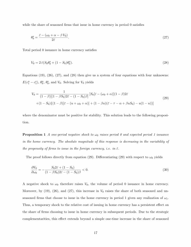
Proposition 1 A one-period negative shock to ω0 raises period 0 and expected period 1 issuance

in the home currency. The absolute magnitude of this response is decreasing in the variability of

the propensity of firms to issue in the foreign currency, i.e. in ε̄.

The proof follows directly from equation (29). Differentiating (29) with respect to ω0 yields

∂V0

∂ω0= − S02ε̄+ (1− S0)

(1− βS0)2ε̄− (1− S0)β< 0. (30)

A negative shock to ω0 therefore raises V0, the volume of period 0 issuance in home currency.

Moreover, by (19), (26), and (27), this increase in V0 raises the share of both seasoned and un-

seasoned firms that choose to issue in the home currency in period 1 given any realization of ω1.

Thus, a temporary shock to the relative cost of issuing in home currency has a persistent effect on

the share of firms choosing to issue in home currency in subsequent periods. Due to the strategic

complementarities, this effect extends beyond a simple one-time increase in the share of seasoned

17

firms.

We relate ωt to countries’ macroeconomic and monetary policies, considering them exogenous to

firm issuance decisions. Extending our model to a multi-country global economy, countries with

better policies, and hence lower ωt on average, will (1) have a larger share of firms issuing in home

currency; and (2) be more likely to be influenced by a temporary decline in ωt due to a change in

global economic circumstances.21

Lastly, we turn to the implications of the variability of firm propensity to issue in foreign currency

for the magnitude of this response. By (30), the cross partial satisfies

∂2V0

∂ω0∂ε̄=

2(1− S0)

[(1− βS0)2ε̄− (1− S0)β]2> 0, (31)

indicating that the more similar the firms, the larger the response to changes in ωt.

Our model therefore makes three testable predictions. First, countries with better economic

fundamentals are likely to have a larger share of bonds issued in their home currency. Second,

given a temporary decline in the relative cost of home currency issuance, countries with sufficiently

sound fundamentals will experience a greater increase in the share of home currency issuance than

countries with worse policies. Such relative advantages could arise from an increase in the cost of

issuing in global currencies, as observed during the global financial crisis. Finally, our cross-partial

results indicate that an increase in ε̄ implies that firms that differ more in their propensity to issue

in foreign currency are less responsive as a group to temporary changes in the relative cost of home

currency issuance. We interpret this result as consistent with our empirical finding that responses

to the crisis were stronger among our financial firm sub-sample, as financial firms are likely more

homogeneous. We test these hypotheses empirically in the next section.

21This is because for countries with better fundamentals prior to the crisis, S0 will be higher and one can showthat ∂2V0/∂ω0∂S0 > 0.

18

4 Empirical analysis

This section proceeds as follows. First we look at the determinants of transition to issuing a higher

share of debt in home currency during and immediately after the global financial crisis. Next we

conduct an issue-level panel analysis to test for potential compositional changes in the set of issuers.

4.1 Country-level analysis

Our model predicts that a discrete global event that temporarily lowers the relative cost of home

currency issuance for all countries will have a persistent positive impact on the share of home

currency issuance for countries with sufficiently sound fundamentals. During the financial crisis,

the relative cost of issuing in one’s own currency likely declined, as markets experienced a dollar

shortage initially, and later, the stability of the euro came into question.22 Moreover, zero or near-

zero policy rates in the U.S., U.K., and euro area resulted in yield-chasing by institutional investors

and increased demand for assets in alternative currencies. As a result, we posit that the crisis

offered firms in countries with sufficiently attractive macroeconomic characteristics an increased

opportunity to issue foreign debt in their own currency.

As we observed in Figure 4, some countries experienced a substantial increase in the share of home

currency issuance after the crisis, while others did not. To understand what factors determined

whether or not a given country experienced an increase in their home currency share of debt, we

estimate the probability of an increase in the average share of home currency issuance between

2002-2006 and 2009-2013 using a cross-country probit model. To control for changes in industry

composition, we compute changes in home currency issuance by country-industry (at SIC2-level)

and estimate the regressions on country-industry cross-section.

We draw upon the original sin literature in specifying macroeconomic covariates. Inflation rates

are likely to be important to investors weighing currency risk. We include a variable indicating

a history of high inflation in the issuer’s country, defined as the number of years since inflation

exceeded 10 percent rate prior to the crisis. We also expect fiscal solvency to impact investors’

22Du and Schreger (2015a) show that local currency spreads on emerging markets’ sovereign bonds declined relativeto foreign currency spreads during the crisis.

19

interest in the country’s currency assets, so we include the debt-to-GDP ratio of the issuer’s country.

We also include interaction of these two variables.23

The results are reported in Table 1. Even though the effect of the change in industry export share

is not significant (column (1)), we find that the regressions have a much better fit if we control

for industry fixed effects (columns (2)-(4)). With industry fixed effects, we find that advanced

economies were more likely to experience an increase in home currency issuance than emerging

economies. However, neither the depth of the crisis, as measured by the GDP decline during the

crisis, nor currency depreciation during the crisis, had an effect. We experimented with a host

of additional macroeconomic variables—both their pre-crisis levels and their changes—but none

altered our main results.

Both “low government debt” and time since high inflation enter our regressions significantly and

in the expected direction. Their interaction reveals that it is the combination of high inflation

and high debt that is detrimental to home currency issuance. For countries with debt less than 48

percent of GDP, inflation history does not matter.24 Alternatively, debt to GDP only matters for

countries that experienced high inflation less than 10 years ago.25

In summary, advanced economies were more likely to experience an increase in home currency

issuance following the global financial crisis as were countries that had both low government debt

and no recent history of high inflation. These results indicate that while fundamentals matter

in manner predicted by the original sin literature, global financial market conditions are also an

important (albeit frequently overlooked) factor explaining original sin. When global currency mar-

kets run smoothly, small currency markets find it difficult to break through; however, when global

currency markets are disrupted, the space for smaller, but stable, currency markets is created.

23For interpretation purposes, in the interaction, the “low debt” variable is measured as 100% minus the debt-to-GDP ratio. In our data, the debt-to-GDP ratio ranges from 8 to 80 percent in 2006.

24The overall effect of inflation history is only significant at 5-percent level if the “low debt” indicator is below52—in other words, if debt is above 48 percent of GDP.

25The overall effect of the low debt indicator is only statistically significant at the 5-percent level if a countryexperienced high inflation in the last 9 years.

20

4.2 Firm-level analysis

Next, we analyze the currency denomination of 16,584 individual bond issues by 2,147 firms from

the 30 non-global currency countries listed in Appendix Table A.1. Issues are denominated in an

issuer’s home currency or a foreign currency, which we assume to be determined by the relative cost

of borrowing in a global versus home currency, rf −rh. Since we cannot observe the counterfactual,

we obviously do not observe this relative cost, and moreover the information on issuance cost is

incomplete in the data. Thus, we have a latent variable model,

I(issue in home currency) =

1 if rf − rh > 0

0 if rf − rh ≤ 0,

rf − rh = X ′β + ε,

where X is a set of explanatory variables that include country fundamentals, issue size, whether

the issuer previously issued in home or foreign currency, as well as a time trend, post-crisis period

indicator, and firm fixed effects. We estimate this model using a linear probability approach

in order to estimate panel regressions with firm fixed effects. Our results, however, are robust to

using conditional logit specifications that allow for firm fixed effects. Since many of our explanatory

variables are country-year level, while our unit of observation is a bond issue, we cluster standard

errors on country-year pairs.

Our model predicts that countries with better fundamentals will have a lower cost of issuing

in home currency, resulting in a larger share of home currency issuance by private firms. Many

differences across countries could account for differences in home currency issuance that are not

captured in our model, such as scale advantages due to country size, quality of contract enforcement,

et cetera. Time-invariant factors are captured by firm fixed effects. Thus, we modify our hypothesis

in dynamic terms: when a country’s fundamentals improve, we expect to observe an increased share

in firm home currency issuance. Because the dynamics are likely to be different across countries,

we separately estimate the effects for advanced and emerging economies in our main regressions.

The results are reported in Table 2, with firm fixed effects included in every regression.

21

In columns (1) and (5) we only include issue-specific variables that, according to our model,

may affect a firm’s probability of issuing in home currency for advanced and emerging economies,

respectively. Consistent with the interpretation of the firm’s idiosyncratic shock ε as the firm’s

export revenues, we find that firms that operate in industries with a higher export share are less

likely to issue in home currency, with the effect statistically significant for advanced economies.

These firms have global currency revenue streams that makes borrowing in global currencies more

attractive. We also find that for firms in both advanced and emerging economies, larger issues are

less likely to be denominated in home currency. There are two reasons for this: first, firms need

a sufficiently deep market to successfully place a large issue; second, larger issues are likely to be

from larger firms, which may be more adept at hedging their positions. In addition, larger firms

are also more likely to be exporters (Melitz, 2003), and given that we are only about to control for

the industry’s export share, part of this effect could be captured in deal size variation.

In the model, we assume that issuing in home currency for the first time is costly. Thus, we

expect issuers seasoned in home currency to be more likely to issue in home currency than issuers

that are not. While our model does not explicitly include a cost associated with issuing in a

global currency for the first time, we might expect such a cost from the literature and our prior

work. Our empirical model therefore includes a cost associated with issuing in any currency for

the first time. Thus, we control for firms’ past experience issuing in both home, and separately in

foreign currency, the omitted benchmark group being new issuers accessing the international bond

market for the first time. The interpretation of these indicators—whether the issuer is seasoned

in home and foreign currencies—is slightly complicated by our firm fixed effects; the coefficients

are identified only by firms that became seasoned during our sample period. Firms in advanced

economies that are seasoned in home currency are more likely to issue in home currency again,

consistent with assumptions in the model.26 For firms in emerging economies, being seasoned in

foreign currency does not affect the probability of issuing in home currency. This may be due to

the fact that only a small number of firms from emerging markets repeatedly borrowed in home

currency. These issue-specific variables, along with firm fixed effects, explain about a third of the

variation in home currency issuance for firms in advanced economies and slightly more than that

26This effect goes away once we include time trend.

22

for firms in emerging economies.

In columns (2) and (6) we add a simple linear trend to test whether the secular trend away

from original sin and towards more home currency issuance in international markets documented

in Figures 2 and 3 is explained by changes in the composition of borrowers. However, even with

firm fixed effects and other issue-specific controls, we still observe a statistically significant upward

trend in home currency issuance. In columns (3) and (7) we test whether this reflects a long-

term trend or a change that occurred since the global financial crisis by including, along with the

trend, a post-crisis indicator. We find no evidence of a secular trend for advanced economies, but

instead an increase in home currency issuance after the global financial crisis. Emerging economies,

by contrast, do appear to have a secular upward trend in home currency issuance, and lack any

detectable crisis-specific effect.

In columns (4) and (8) we add country-specific characteristics to understand the role of macroe-

conomic fundamentals. Included are the same variables we found important in our cross-section

analysis—the government debt to GDP ratio and a history of high inflation. Here, a history of

high inflation is a binary variable that indicates whether that country had at least one year in the

previous 10 where the average inflation rate exceeded 10 percent. This results in a simple inter-

pretation of the interaction between these variables, which we include to allow for high inflation

to have a differential effect co-dependent on the level of fiscal debt. We experimented with a host

of additional macroeconomic variables that could potentially impact the probability of issuing in

home currency, but did not find robust results. Most notably, controlling for inflation history, we

did not find an effect specific to explicit inflation target policies.

Our results suggest that short-term macroeconomic fundamentals matter only for issuance de-

cisions in advanced economies. For these countries, the higher is the government debt, the more

important is the history of inflation. In particular, with debt-to-GDP ratio exceeding 49 percent, a

history of high inflation negatively affects the probability of firms issuing in home currency.27 We

don’t observe any effects of macroeconomic fundamentals for firms in emerging economies .

27The total effect of high inflation for countries with a debt to GDP ratio of 38 percent or more is negative andbecomes statistically significant at 5 percent level when the debt-to-GDP ratio reaches49 percent.

23

4.3 Issuer heterogeneity

Our data allow us to distinguish between two important sets of borrowers: financial and non-

financial companies. These two groups differ in many ways and frequently the markets for financial

and non-financial companies’ bonds are viewed as separate. One important distinction from the

point of view of our model predictions, is that financial firms are much more homogeneous. Our

model predicts that a bond market with firms that are more homogeneous will be more sensitive

to exogenous changes in relative issuance costs.

To test this prediction, we divide our data into issues by financial firms–including those that are

part of large vertical conglomerates–and issues by non-financial firms. We repeat our analysis with

firm fixed effects and report our main regressions in Table 3. We find that our main results are

mostly driven by bonds issued by financial firms from advanced economies (column (1)) — only

for this group do we observe a positive increase in home currency issuance in the aftermath of the

global financial crisis and sensitivity to better fundamentals.

For non-financial firms from advanced economies as well as for financial firms from emerging

economies we observe a small secular trend towards increased home currency issuance (columns (2)

and (3)). For financial firms from emerging economies we in fact observe a slowdown in the trend

after the global financial crisis.

As before, we find that larger issues are less likely to be denominated in home currency. We also

find that financial firms that are parts of corporations that are in exporting sectors are less likely

to issue in home currency, also consistent with our model.

Together, these results indicate that both global financial market conditions and macroeconomic

fundamentals influence an advanced economy firm’s ability to borrow internationally in its home

currency. While idiosyncratic firm factors account for the probability that firms borrow abroad in

home currency in all countries, only in advanced economies do we observe a statistically significant

increase in home currency issuance following the global financial crisis. This probability is higher

if a firm’s home country does not have a combination of high debt-to-GDP and a history of high

inflation, and is driven by the financial firms in our sample, which are more homogeneous than

the non-financial firms. In emerging economies, macroeconomic fundamentals are still by and large

24

below the threshold that would allow for a substantial increase in home currency issuance from

an event such as the global financial crisis, but we observe a small secular upward trend in home

currency issuance by emerging market firms as well.

4.4 Robustness tests

We conducted a number of robustness tests for the regressions that produce our main results —

firm-level regressions for advanced economies, all firms and financial firms only, reported in column

(4) of Table 2 and column (1) of Table 3, respectively. The results are presented in Appendix Table

A.4.

Our first test is whether our regressions are misspecified in terms of the underlying error dis-

tribution because we estimate a linear probability regression specification. Since our benchmark

regressions include firm fixed effects, probit version of this regression is not identified, however, we

can estimate a conditional logit regression. We can see from columns (1) and (2) that our results

remain qualitatively unchanged, for both full sample of firms and for financial firms only.28

Our next test is whether our results are driven by specific countries included in our sample. One

country that tends to stand out is China, which experienced a number of economic changes during

our sample period, including increased bond issuance, for reasons that are largely orthogonal to our

model’s argument. China is included in the group of emerging economies in our analysis, thus, it

cannot be driving the results for advanced economies. Another country that stands out specifically

in our analysis, is Sweden, in that we observe a large increase in Swedish kronor denominated bonds.

We want to make sure that Sweden is not the only country that drives our results. Excluding it from

the sample, we observe from columns (3) and (4) that the results remain qualitatively unchanged,

but are in fact larger in magnitude and more statistically significant.

In the paper we focused exclusively on bonds issued by private firms, financial and non-financial.

We find that including sovereign bond issues in the sample does not alter our results (column (5)).

However, when we conduct similar analysis for sovereign issues only, we do not find any significant

results (column (6)). This is because our data source only includes bonds that are issued explicitly

28Magnitudes of coefficients are, of course, different, because they have different interpretation.

25

in international markets and in recent years sovereign were issuing more in domestic markets in

both home and foreign currencies, while allowing foreign investors access to these markets (Du and

Schreger, 2015b).

Finally, we are concerned that there is heterogeneity with respect to foreign ownership of bond

issuers and want to make sure foreign-owned firms don’t drive our results. Thus, for our final

robustness test, we exclude all borrowers that have foreign parents (regardless of parent nationality,

as long as it is not the same as borrower nationality), which contribute about 13 percent to the

total number of bond issues in our regressions. As we can see from columns (7) and (8), the results

remain unchanged.

5 Conclusion

The evidence presented above demonstrates a reduction in the incidence of original sin in a large

sample of individual foreign bond issuances, highlighting the role of macroeconomic conditions that

explain a country’s propensity to overcome original sin and begin issuing foreign bonds denominated

in their home currencies. Furthermore, we hypothesize that the global financial crisis of 2008-2009

offered countries with sufficiently attractive macroeconomic characteristics a “baptism” of sorts.

This set the stage for a new equilibrium in the global economy—one in which a broader set of

countries are able to issue debt internationally in their own currency. We find that those countries

that were able to take advantage of the temporary disruption and near-zero interest rates in global

financial markets were the ones with a combination of low government debt and a history of

stable inflation. These macroeconomic characteristics are consistent with the channels highlighted

in the original sin literature, namely the costliness of default on home currency debt through

higher inflation. Advanced economies with lower government debt and inflation were more likely

to increase home currency foreign bond issuance during our sample period. These characteristics

were insignificant for emerging economies, however. As a group, these countries’ fundamentals

still appear to be on average below the threshold at which improved domestic macroeconomic

characteristics could result in an observable increase in the incidence of home currency issuance.

Our paper also contributes to the discussion of global reserve currency dominance, as our data

26

indicates a decline in the role of global currencies in the international bond market. Going forward,

many anticipate the end of a dollar-dominated global monetary system. Before the crisis, based on

factors such as home market size, available liquidity, and rates of return, Chinn and Frankel (2008)

predicted that the euro could surpass the U.S. dollar as the dominant global reserve currency by

2015.

A related issue is whether the international financial system is moving away from reserve-currency

dominance. Eichengreen and Flandreau (2012) argue that it was desirable policies, not scale

economies, that led to the ascent of the dollar at the expense of the British sterling. Prior to

that, these currencies shared the reserve currency relatively equally [Eichengreen and Flandreau

(2009)]. A number of studies envision a multi-polar world going forward, with a non-trivial re-

gional role for the renminbi [e.g. Dobson and Masson (2008) and Eichengreen (2012)]. This stance

remains controversial as the dollar’s inertial advantages are likely to maintain its preeminence as

the sole global currency for some time to come (Goldberg, 2010). For example, the severe dollar

funding needs of foreign banks during the global financial crisis demonstrated that the dollar was

still the reserve currency as recently as 2008-2009. That said, it is apparent that firms from ad-

vanced countries now issue a larger proportion of their debt in their home currency than they did

previously.

27

References

Alfaro, L. and Kanczuk, F. (2013). Debt redemption and reserve accumulation. NBER WP 19098.

Bacchetta, P. and Merrouche, O. (2015). Countercyclical foreign currency borrowing: Eurozonefirms in 2007-2009. Swiss Finance Institute Research Paper No. 15-63.

Burger, J. D., Sengupta, R., and Warnock, Francis E., W. V. C. (2015). U.s. investment in globalbond markets: As the fed pushes, some emes pull. Economic Policy, 30(84):729–766.

Burger, J. D. and Warnock, F. E. (2006). Local currency bond markets. IMF Staff Papers, 53:115–132.

Burger, J. D. and Warnock, Francis E., W. V. C. (2012). Emerging local currency bond markets.Financial Analysis Journal, 68(4):73–93.

Caballero, R. and Farhi, E. (2013). A model of the safe asset mechanism (sam): Safety traps andeconomic policy. NBER WP 18737.

Calvo, G., Izquierdo, A., and L.F., M. (2008). Systemic sudden stops: The relevance of balance-sheet effects and financial integration. NBER WP 14026.

Chinn, M. and Frankel, J. (2008). Why the euro will rival the dollar. International Finance,11(1):49–73.

Dobson, W. and Masson, P. R. (2008). When will the renminbi become a world currency? ChinaEconomic Review, 20:124–135.

Du, W. and Schreger, J. (2015a). Local currency sovereign risk. Journal of Finance, forthcoming.

Du, W. and Schreger, J. (2015b). Sovereign risk, currency risk, and corporate balance sheets.mimeo.

Eichengreen, B. (2012). International liquidity in a multipolar world. American Economic Review,102(3):207–212.

Eichengreen, B. and Flandreau, M. (2009). The rise and fall of the dollar, or when did the dollarreplace sterling as the leading reserve currency? European Review of Economic History, 63:666–694.

Eichengreen, B. and Flandreau, M. (2012). The federal reserve, the bank of england and the riseof the dollar as an international currency, 1914-39. Open Economies Review, 23(1):57–87.

Eichengreen, B. and Hausmann, R. (1999). Exchange rates and financial fragility. NBER WorkingPapers: 7418.

Eichengreen, B., Hausmann, R., and Panizza, U. (2007). Currency mismatches, debt intolerance,and the original sin: Why they are not the same and why it matters. In Capital Controls andCapital Flows in Emerging Economies: Policies, Practices and Consequences, pages 121–170.National Bureau of Economic Research, Inc. and Chicago University Press.

Goldberg, L. (2010). Is the international role of the dollar changing? FRBNY Current Issues,16(1):1–7.

28

Hale, G. B. and Spiegel, M. M. (2012). Currency composition of international bonds: The emueffect. Journal of International Economics, 88:134–149.

Hausmann, R. and Panizza, U. (2003). On the determinants of original sin: An empirical investi-gation. Journal of international Money and Finance, 22:957–990.

Hausmann, R. and Panizza, U. (2011). Redemption or abstinence? original sin, currency mis-matches and counter cyclical policies in the new millennium. Journal of Globalization and De-velopment, 2(1).

Krugman, P. (1999). Balance sheets, the transfer problem, and financial crises. In Isard, P., Razin,A., and Rose, A. K., editors, International finance and financial crises: Essays in honor of RobertP. Flood, Jr., pages 31–44. Kluwer Academic Publishers and International Monetary Fund.

McCauley, R., McGuire, P., and Sushko, V. (2015). Dollar credit to emerging market economies.BIS Quarterly Review.

Melitz, M. J. (2003). The impact of trade on intra–industry reallocations and aggregate industryproductivity. Econometrica, 71:1695–1725.

Rose, A. (2007). A stable international monetary system emerges: Inflation targeting is brettonwoods, reversed. Journal of International Money and Finance, 26:663–691.

Schneider, M. and Tornell, A. (2004). Balance sheet effects, bailout guarantees and financial crises.The Review of Economic Studies, 71(3).

29

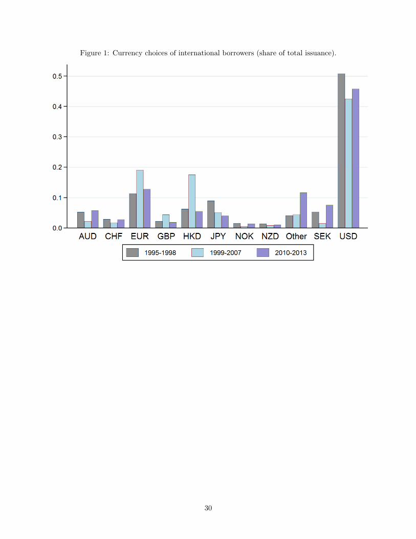
Figure 1: Currency choices of international borrowers (share of total issuance).

30

Figure 2: Bond issuance by currency and country group.

 

31

Figure 3: Share of number of bonds issued in home currencyby firm’s prior experience and country group.

 

32

Figure 4: Change in the share of bonds issued in home currency between 2002-2006 and 2009-2013.

33

Table 1: Cross-section regressions:Probability of increase in the ratio of home currency issuance.

(1) (2) (3) (4)

Years Since Infl. >10% (a) 0.34*** 0.68*** 0.66*** 0.64**

(0.12) (0.23) (0.24) (0.28)

100% - Debt / GDP (b) 0.12*** 0.23** 0.23** 0.23**

(0.046) (0.095) (0.094) (0.11)

(a) ∗ (b) -0.0057*** -0.012*** -0.012*** -0.011**

(0.002) (0.0042) (0.0042) (0.0047)

Advanced economy 0.77 2.22** 2.53*** 2.56***

(0.56) (0.88) (0.91) (0.90)

Change in industry export sharec 0.16

(3.58)

Real GDP decline (crisis)d -0.86 -1.02

(1.27) (1.6)

Currency depreciation (crisis)e -0.40

(1.38)

Industry FEs No Yes Yes Yes

Observations 42 34 34 34

Pseudo R2 0.23 0.66 0.67 0.67

Unit of observation is country-industry (SIC2). Dependent variable is equal to 1 if the share

of home currency bonds increased from 2002-2006 average to 2009-2013 average, 0 otherwise.

Probit regression. Only countries with at least 10 issues in 2002-2006 and in 2009-2013

are included in the regressions. *(P< 0.10), **(P< 0.05), ***(P< 0.01).aNumber of years since inflation exceeded 10 percent before 2006.bDebt is Gross government debt. Debt/GDP ratio is as of 2006.cChange in industry export share from average in 2002-06 to average 2009-13.dReal GDP decline (crisis) is cumulative percentage points decline in GDP in 2007-08.eCurrency depreciation (crisis) is cumulative percentage points depreciation against USD in 2007-08.

34

Table 2: Issue-Level Regressions: Probability of Home Currency Issuance.

Advanced Economies Emerging Economies

(1) (2) (3) (4) (5) (6) (7) (8)

Trend 0.0093*** -0.00018 -0.003 0.0081*** 0.012** 0.012**

(0.0023) (0.0028) (0.0029) (0.0031) (0.0049) (0.0049)

Post Crisis 0.11*** 0.12*** -0.042 -0.043

(0.026) (0.034) (0.028) (0.028)

High inflation (a) 0.25* -0.011

(0.14) (0.065)

Debt / GDP 0.00071 -0.00075

(0.0011) (0.00097)

(a) ∗ (b) -0.0069*** -0.000017

(0.0025) (0.00095)

Export Share -0.41** -0.34** -0.33** -0.34** -0.061 -0.067 -0.079 -0.053

(0.16) (0.16) (0.16) (0.16) (0.062) (0.080) (0.093) (0.093)

Deal Amount -0.15*** -0.16*** -0.17*** -0.17*** -0.098* -0.12** -0.12** -0.13**

(0.037) (0.038) (0.038) (0.040) (0.057) (0.056) (0.055) (0.056)

Seasoned Dom. Cur. 0.066*** 0.019 0.0031 -0.0075 -0.14 -0.16** -0.16** -0.16**

(0.016) (0.015) (0.016) (0.018) (0.086) (0.081) (0.081) (0.081)

Seasoned For. Cur. -0.009 -0.036* -0.021 -0.018 0.020 -0.00011 0.00021 -0.0015

(0.02) (0.02) (0.019) (0.018) (0.014) (0.015) (0.015) (0.015)

Observations 14020 14020 14020 14020 2564 2564 2564 2564

Adjusted R2 0.30 0.31 0.32 0.32 0.39 0.39 0.39 0.39

Unit of observation is an individual bond issue. Dependent variable is equal to 1 if issue

is denominated in home currency, 0 otherwise. Linear probability model with firm fixed effects.(a)Recent high inflation = 1 if inflation over 10 percent was observed in last 10 years,

0 otherwise. (b)Debt is gross government debt. Regressions include firm FEs.

Robust standard errors clustered on country-year. *(P< 0.10), **(P< 0.05), ***(P< 0.01).

35

Table 3: Issue-Level Regressions: Probability of Home Currency Issuance: Financial and non-financial firms.

Advanced Economies Emerging Economies

FIN non-FIN FIN non-FIN

(1) (2) (3) (4)

Trend -0.0045 0.019* 0.017** 0.0051

(0.0032) (0.011) (0.0070) (0.0053)

Post Crisis 0.13*** -0.039 -0.061* -0.026

(0.038) (0.12) (0.037) (0.051)

High inflation (a) 0.24* 0.54 0.0062 -0.042

(0.14) (0.74) (0.10) (0.093)

Debt / GDP (b) 0.00073 0.0018 -0.00091 -0.00058

(0.0012) (0.0028) (0.0014) (0.0025)

(a) ∗ (b) -0.0067*** -0.011 0.00004 -0.00019

(0.0025) (0.011) (0.0015) (0.0024)

Export Share -0.39** -0.18 0.044 -0.45

(0.17) (0.25) (0.046) (0.35)

Deal Amount -0.16*** -0.50*** -0.13** -0.082

(0.037) (0.16) (0.056) (0.15)

Seasoned Dom. Cur. -0.14 0.10 -0.14 -0.24

(0.018) (0.087) (0.097) (0.17)

Seasoned For. Cur. -0.036 -0.039 -0.014 0.022

(0.027) (0.034) (0.018) (0.025)

Observations 12474 1546 1505 1059

Adjusted R2 0.31 0.42 0.31 0.48

Unit of observation is an individual bond issue. Dependent variable is equal to 1 if issue

is denominated in home currency, 0 otherwise. Linear probability model with firm fixed effects.(a)Recent high inflation = 1 if inflation over 10 percent was observed in last 10 years,

0 otherwise. (b)Debt is gross government debt. Regressions include firm FEs.

FIN = firm is listed as a financial sector firm, including financial divisions of corporates.

Robust standard errors clustered on country-year. *(P< 0.10), **(P< 0.05), ***(P< 0.01).

36

A Appendix

Table A.1: Countries in the sample by country group.

Advanced Emerging

Australia Argentina Kazakhstan Turkey

Canada Brazil Malaysia Thailanda

Denmark Chile Mexico Ukraine

Icelanda China Perua

Korea Colombiaa Philippines

New Zealand Czech Republica Polanda

Norway Hungary Romaniaa

Sweden India Russian Federation

Taiwana Indonesia South Africa

aOmitted from cross section regression, due to insufficient sample size.

37

Table A.2: Issues and amount by year and country group.

Number of Issues Amount (Real USD Bila)

Year Emerging Advanced Emerging Advanced

1995 13 211 1.5 16.3

1996 59 364 5.4 29.4

1997 81 403 8.2 33.9

1998 56 335 6.2 32.4

1999 39 392 4.0 41.6

2000 77 453 6.3 35.0

2001 84 636 7.2 46.0

2002 66 676 5.5 43.8

2003 124 800 14.9 56.0

2004 136 1015 18.8 66.6

2005 169 908 21.4 72.8

2006 236 1001 23.3 96.1

2007 207 1191 27.6 95.2

2008 82 1044 9.1 111.0

2009 106 1010 21.6 110.4

2010 216 1059 38.0 109.3

2011 200 748 30.2 84.1

2012 263 984 44.7 108.1

2013 350 790 51.9 86.1

Total 2564 14020 345.8 1274.2

aBase 1982-1984.

38

Table A.3: Summary statistics by country group.

N Mean Std. Dev. Min. Max

Advanced (9 Countries)

Home currency issue 14020 0.11 0.32 0 1

Deal amount (Bil. real USD)a 14020 0.09 0.16 0.00 2.32

Seasoned home cur. issuer 14020 0.68 0.47 0 1

Seasoned for. cur. issuer 14020 0.93 0.25 0 1

Gross govt. debt/GDP 14020 36.81 24.46 8.6 101.7

Inflation >10% last 10 years 14020 0.03 0.18 0 1

Emerging (21 Countries)

Home currency issue 2564 0.06 0.24 0 1

Deal amount (Bil. real USD)a 2564 0.13 0.13 0.00 1.40

Seasoned home cur. issuer 2564 0.07 0.25 0 1

Seasoned for. cur. issuer 2564 0.58 0.49 0 1

Gross govt. debt/GDP 2564 40.41 22.60 3.8 139.4

Inflation >10% last 10 years 2564 0.75 0.43 0 1aBase 1982-1984.

39

Table A.4: Issue-Level Regressions: Probability of Home Currency Issuance: Advanced economies.Robustness tests.

Conditional Logit Exclude Sweden Include Only Exclude foreign-owned

All FIN All FIN sovereign sovereign All FIN

(1) (2) (3) (4) (5) (6) (7) (8)

Trend -0.041 -0.072 -0.0009 -0.0025 -0.0032 -0.0019 -0.0029 -0.0045

(0.088) (0.11) (0.0019) (0.0019) (0.0029) (0.0027) (0.0029) (0.0032)

Post Crisis 1.66*** 1.92*** 0.049*** 0.053*** 0.12*** 0.046 0.12*** 0.13***

(0.63) (0.72) (0.016) (0.016) (0.034) (0.049) (0.035) (0.039)

High inflation (a) 6.86** 6.16** 0.90** 1.08*** 0.15 0.065 0.18 0.19

(3.28) (2.99) (0.36) (0.36) (0.14) (0.099) (0.13) (0.13)

Debt / GDP (b) 0.033 0.032 0.0037*** 0.0039*** 0.0006 -0.0001 0.0004 0.0004

(0.07) (0.077) (0.0006) (0.0006) (0.0011) (0.0005) (0.0011) (0.0012)

(a) ∗ (b) -0.16*** -0.15*** -0.021** -0.026*** -0.0049** -0.0012 -0.0056** -0.0058**

(0.06) (0.055) (0.008) (0.008) (0.002) (0.0017) (0.0024) (0.0024)

Export Share -2.82 -4.37 -0.35** -0.40** -0.34** -0.32 -0.64

(9.92) (23.3) (0.17) (0.18) (0.16) (0.29) (0.47)

Deal Amount -3.56*** -3.18*** -0.062*** -0.062*** -0.16*** -0.0067 -0.17*** -0.16***

(0.95) (0.80) (0.022) (0.022) (0.037) (0.008) (0.040) (0.038)

Seasoned 0.23 0.15 -0.044*** -0.042*** -0.006 -0.037 -0.0023 -0.011

Dom. Cur. (0.86) (1.06) (0.014) (0.013) (0.018) (0.038) (0.019) (0.019)

Seasoned -0.33 -0.41 -0.003 -0.038 -0.017 0.007 0.009

For. Cur. (2.29) (3.17) (0.019) (0.030) (0.018) (0.018) (0.022)

Observations 11200 10823 11265 10011 14333 313 12255 10948

Adjusted R2 0.331 0.310 0.323 0.00817 0.266 0.237

Unit of observation is an individual bond issue. Dependent variable is equal to 1 if issue

is denominated in home currency, 0 otherwise. Linear probability model with firm fixed effects.(a)Recent high inflation = 1 if inflation over 10 percent was observed in last 10 years,

0 otherwise. (b)Debt is gross government debt. Regressions include firm FEs.

Advanced economies only, the sample of firms as indicated.

FIN = firm is listed as a financial sector firm, including financial divisions of corporates.

Robust standard errors clustered on country-year. *(P< 0.10), **(P< 0.05), ***(P< 0.01).

40