The Riemann Zeta Function

David Jekel

June 6, 2013

In 1859, Bernhard Riemann published an eight-page paper, in which heestimated “the number of prime numbers less than a given magnitude” usinga certain meromorphic function on C. But Riemann did not fully explainhis proofs; it took decades for mathematicians to verify his results, and tothis day we have not proved some of his estimates on the roots of ξ. EvenRiemann did not prove that all the zeros of ξ lie on the line Re(z) = 1

2 . Thisconjecture is called the Riemann hypothesis and is considered by many thegreatest unsolved problem in mathematics.

H. M. Edwards’ book Riemann’s Zeta Function [1] explains the histor-ical context of Riemann’s paper, Riemann’s methods and results, and thesubsequent work that has been done to verify and extend Riemann’s theory.The first chapter gives historical background and explains each section ofRiemann’s paper. The rest of the book traces later historical developmentsand justifies Riemann’s statements.

This paper will summarize the first three chapters of Edwards. Mypaper can serve as an introduction to Riemann’s zeta function, with proofsof some of the main formulae, for advanced undergraduates familiar withthe rudiments of complex analysis. I use the term “summarize” loosely;in some sections my discussion will actually include more explanation andjustification, while in others I will only give the main points. The paperwill focus on Riemann’s definition of ζ, the functional equation, and therelationship between ζ and primes, culminating in a thorough discussion ofvon Mangoldt’s formula.

1

Contents

1 Preliminaries 3

2 Definition of the Zeta Function 32.1 Motivation: The Dirichlet Series . . . . . . . . . . . . . . . . 42.2 Integral Formula . . . . . . . . . . . . . . . . . . . . . . . . . 42.3 Definition of ζ . . . . . . . . . . . . . . . . . . . . . . . . . . . 5

3 The Functional Equation 63.1 First Proof . . . . . . . . . . . . . . . . . . . . . . . . . . . . 73.2 Second Proof . . . . . . . . . . . . . . . . . . . . . . . . . . . 8

4 ξ and its Product Expansion 94.1 The Product Expansion . . . . . . . . . . . . . . . . . . . . . 94.2 Proof by Hadamard’s Theorem . . . . . . . . . . . . . . . . . 10

5 Zeta and Primes: Euler’s Product Formula 12

6 Riemann’s Main Formula: Summary 13

7 Von Mangoldt’s Formula 157.1 First Evaluation of the Integral . . . . . . . . . . . . . . . . . 157.2 Second Evaluation of the Integral . . . . . . . . . . . . . . . . 177.3 Termwise Evaluation over ρ . . . . . . . . . . . . . . . . . . . 197.4 Von Mangoldt’s and Riemann’s Formulae . . . . . . . . . . . 22

2

1 Preliminaries

Before we get to the zeta function itself, I will state, without proof, someresults which are important for the later discussion. I collect them here sosubsequent proofs will have less clutter. The impatient reader may skip thissection and refer back to it as needed.

In order to define the zeta function, we need the gamma function, whichextends the factorial function to a meromorphic function on C. Like Edwardsand Riemann, I will not use the now standard notation Γ(s) where Γ(n) =(n−1)!, but instead I will call the function Π(s) and Π(n), will be n!. I givea definition and some identities of Π, as listed in Edwards section 1.3.

Definition 1. For all s ∈ C except negative integers,

Π(s) = limN→∞

(N + 1)sN∏n=1

n

s+ n.

Theorem 2. For Re(s) > −1, Π(s) =∫∞0 e−xxs dx.

Theorem 3. Π satisfies

1. Π(s) =∏∞n=1(1 + s/n)−1(1 + 1/n)s

2. Π(s) = sΠ(s− 1)

3. Π(s)Π(−s) sinπs = πs

4. Π(s) = 2√πΠ(s/2)Π(s/2− 1/2).

Since we will often be interchanging summation and integration, thefollowing theorem on absolute convergence is useful. It is a consequence ofthe dominated convergence theorem.

Theorem 4. Suppose fn is nonnegative and integrable on compact sub-sets of [0,∞). If

∑fn converges and

∫∞0

∑fn converges, then

∑∫∞0 fn =∫∞

0

∑fn.

2 Definition of the Zeta Function

Here I summarize Edwards section 1.4 and give additional explanation andjustification.

3

2.1 Motivation: The Dirichlet Series

Dirichlet defined ζ(s) =∑∞

n=1 n−s for Re(s) > 1. Riemann wanted a def-

inition valid for all s ∈ C, which would be equivalent to Dirichlet’s forRe(s) > 1. He found a new formula for the Dirichlet series as follows. ForRe(s) > 1, by Euler’s integral formula for Π(s) 2,∫ ∞

0e−nxxs−1 dx =

1

ns

∫ ∞0

e−xxs−1 dx =Π(s− 1)

ns.

Summing over n and applying the formula for a geometric series gives

Π(s− 1)∞∑n=1

1

ns=∞∑n=1

∫ ∞0

e−nxxs−1 dx =

∫ ∞0

e−xxs−1

1− e−xdx =

∫ ∞0

xs−1

ex − 1dx.

We are justified in interchanging summation and integration by Theorem 4because the integral on the right converges at both endpoints. As x → 0+,ex−1 behaves like x, so that the integral behaves like

∫ a0 x

s−2 dx which con-verges for Re(s) > 1. The integral converges at the right endpoint becauseex grows faster than any power of x.

2.2 Integral Formula

To extend this formula to C, Riemann integrates (−z)s/(ez − 1) over a thepath of integration C which “starts” at +∞, moves to the origin along the“top” of the positive real axis, circles the origin counterclockwise in a smallcircle, then returns to +∞ along the “bottom” of the positive real axis.That is, for small positive δ,∫

C

(−z)s

ez − 1

dz

z=

(∫ δ

+∞+

∫|z|=δ

+

∫ +∞

δ

)(−z)s

ez − 1

dz

z.

Notice that the definition of (−z)s implicitly depends on the definitionof log(−z) = log |z| + i arg(−z). In the first integral, when −z lies onthe negative real axis, we take arg(−z) = −πi. In the second integral,the path of integration starts at z = δ or −z = −δ, and as −z proceedscounterclockwise around the circle, arg(−z) increases from −πi to πi. (Youcan think of the imaginary part of the log function as spiral staircase, andgoing counterclockwise around the origin as having brought us up one level.)In the last integral, arg(−z) = πi. (Thus, the first and last integrals do not

4

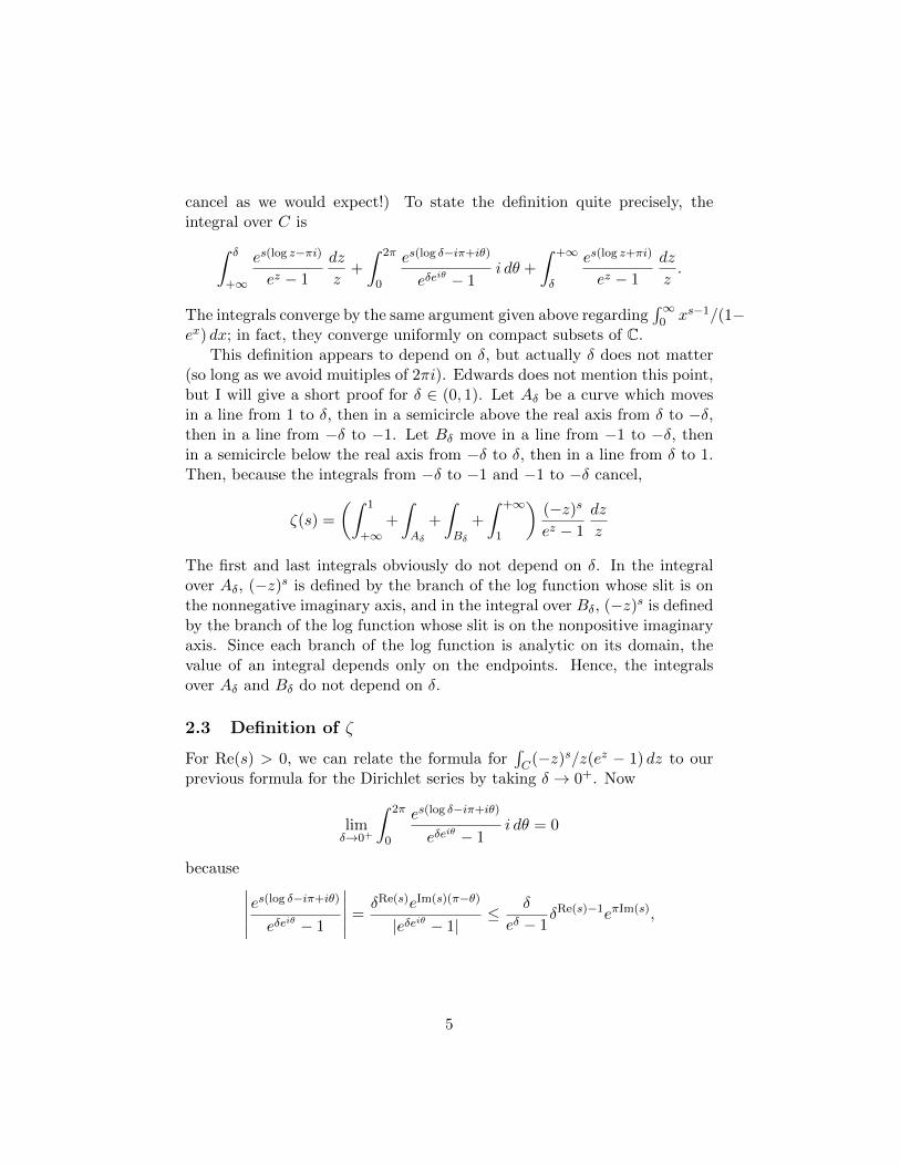
cancel as we would expect!) To state the definition quite precisely, theintegral over C is∫ δ

+∞

es(log z−πi)

ez − 1

dz

z+

∫ 2π

0

es(log δ−iπ+iθ)

eδeiθ − 1i dθ +

∫ +∞

δ

es(log z+πi)

ez − 1

dz

z.

The integrals converge by the same argument given above regarding∫∞0 xs−1/(1−

ex) dx; in fact, they converge uniformly on compact subsets of C.This definition appears to depend on δ, but actually δ does not matter

(so long as we avoid muitiples of 2πi). Edwards does not mention this point,but I will give a short proof for δ ∈ (0, 1). Let Aδ be a curve which movesin a line from 1 to δ, then in a semicircle above the real axis from δ to −δ,then in a line from −δ to −1. Let Bδ move in a line from −1 to −δ, thenin a semicircle below the real axis from −δ to δ, then in a line from δ to 1.Then, because the integrals from −δ to −1 and −1 to −δ cancel,

ζ(s) =

(∫ 1

+∞+

∫Aδ

+

∫Bδ

+

∫ +∞

1

)(−z)s

ez − 1

dz

z

The first and last integrals obviously do not depend on δ. In the integralover Aδ, (−z)s is defined by the branch of the log function whose slit is onthe nonnegative imaginary axis, and in the integral over Bδ, (−z)s is definedby the branch of the log function whose slit is on the nonpositive imaginaryaxis. Since each branch of the log function is analytic on its domain, thevalue of an integral depends only on the endpoints. Hence, the integralsover Aδ and Bδ do not depend on δ.

2.3 Definition of ζ

For Re(s) > 0, we can relate the formula for∫C(−z)s/z(ez − 1) dz to our

previous formula for the Dirichlet series by taking δ → 0+. Now

limδ→0+

∫ 2π

0

es(log δ−iπ+iθ)

eδeiθ − 1i dθ = 0

because ∣∣∣∣∣es(log δ−iπ+iθ)eδeiθ − 1

∣∣∣∣∣ =δRe(s)eIm(s)(π−θ)

|eδeiθ − 1|≤ δ

eδ − 1δRe(s)−1eπIm(s),

5

but δ/(eδ − 1)→ 1 and δRe(s)−1 → 0. Hence,∫C

(−z)s

ez − 1

dz

z= lim

δ→0+

(∫ δ

+∞

es(log z−πi)

ez − 1

dz

z+

∫ +∞

δ

es(log z+πi)

ez − 1

dz

z

)

= (eiπs − e−iπs)∫ ∞0

zs−1

ez − 1dz.

But this integral is exactly Π(s− 1)∑∞

n=1 n−s. Therefore, for Re(s) > 1,

∞∑n=1

1

ns=

1

2i(sinπs)Π(s− 1)

∫C

(−z)s

ez − 1

dz

z

By Theorem 3, 1/2i(sinπs)Π(s − 1) = Π(−s)/2πi. Therefore, Riemanngives the following definition of the zeta function, which coincides with theDirichlet series for Re(s) > 1:

Definition 5. ζ(s) =Π(−s)

2πi

∫C

(−z)s

ez − 1

dz

z.

Theorem 6. For Re(s) > 1, ζ(s) =

∞∑n=1

1

ns.

The integral over C converges uniformly on compact subsets of C becauseez grows faster than any power of z. It follows that the integral defines ananalytic function. Thus, ζ is analytic except possibly at the positive integerswhere Π(−s) has poles. Because the Dirichlet series converges uniformly onRe(s) > 1+δ for any positive δ, we see ζ is actually analytic for s = 2, 3, 4 . . . ,and it is not too hard to check that the integral has a zero there which cancelsthe pole of Π. Thus, ζ is analytic everywhere except 1 where it has a simplepole.

3 The Functional Equation

Riemann derives a functional equation for ζ, which states that a certainexpression is unchanged by the substitution of 1− s for s.

Theorem 7. Π(s

2− 1)π−s/2ζ(s) = Π

(1− s

2− 1

)π−1/2+s/2ζ(1− s).

He gives two proofs of this functional equation, both of which Edwardsdiscusses (sections 1.6 and 1.7). I will spend more time on the first.

6

3.1 First Proof

Fix s < 1. Let DN = {z : δ < |z| < (2N + 1)π} \ (δ, (2N + 1)π). Weconsider Dn split along the positive real axis. Let CN be the same contouras C above except that the starting and ending point is (2N + 1)π ratherthan +∞. Then∫

∂DN

(−z)s

ez − 1

dz

z=

∫|z|=(2N+1)π

(−z)s

ez − 1

dz

z−∫CN

(−z)s

ez − 1

dz

z.

We make similar stipulations as before regarding the definition of log(−z);that is, arg(−z) is taken to be −πi on the “top” of the positive real axis and−πi on the “bottom.” Note that the integrand is analytic except at polesat 2πin. If log z were analytic everywhere, the residue theorem would give∫

∂DN

(−z)s

ez − 1

dz

z= 2πi

∑z∈Dn

Res

((−z)s

z(ez − 1), z

).

In fact, we can argue that this is still the case by spliting Dn into two piecesand considering an analytic branch of the log function on each piece. Thisargument is similar to the one made in the last section and is left to thereader.

The residue at each point 2πin for integer n 6= 0 is computed by inte-grating over a circle of radius r < 2π:

1

2πi

∫|z−2πin|=r

(−z)s

ez − 1

dz

z= − 1

2πi

∫|z−2πin|=r

(−z)s−1 z − 2πin

ez − 1

dz

z − 2πin.

Since (−z)s−1 is analytic at z = 2πin and (z − 2πin)/(ez − 1) has a remov-able singularity (its limit is 1), we can apply Cauchy’s integral formula toconclude that the residue is −(−2πin)s−1. Hence,∫CN

(−z)s

ez − 1

dz

z=

∫|z|=(2N+1)π

(−z)s

ez − 1

dz

z+2πi

N∑n=1

((−2πin)s−1 + (2πin)s−1

).

As we take N → ∞, the left side approaches the integral over C. I claimthe integral on the right approaches zero. Notice 1/(1 − ez) is bounded on|z| = (2N + 1)π. For if |Re(z)| > π/2, then |ez − 1| ≥ 1 − eπ/2 by thereverse triangle inequality. If |Im(z) − 2πin| > π/2 for all integers n, then|ez − 1| > 1 because Im(ez) < 0. For |z| = (2N + 1)π, at least one of thesetwo conditions holds. The length of the path of integration is 2π(2N + 1)π

7

and |(−z)s/z| ≤ (2N + 1)s−1, so the whole integral is less than a constanttimes (2N + 1)s, which goes to zero as N →∞ because we assumed s < 0.

Therefore, taking N →∞ gives∫C

(−z)s

ez − 1

dz

z= 2πi(2π)s−1(is−1 + (−i)s−1)

∞∑n=1

ns−1.

From our definition of the log function,

is−1 + (−i)s−1 =1

i(is − (−i)s) =

1

i(eπis/2 − e−πis/2) = 2 sin

πs

2.

Substituting this into the previous equation and multiplying by Π(−s)/2πigives

ζ(s) = Π(−s)(2π)s−1(

2 sinπs

2

)ζ(1− s), s < 0.

Applying various identities of Π from Theorem 3 will put this equation intothe form given in the statement of the theorem. Since the equation holdsfor s < 0 and the functions involved are all analytic on C except for somepoles at certain integers, the equation holds on all of C \ Z.

3.2 Second Proof

The second proof I will merely summarize. Riemann applies a change ofvariables in the integral for Π to obtain

1

nsπ−s/2Π

(s2− 1)

=

∫ ∞0

e−n2πxxs/2−1 dx, Re(s) > 1.

Summing this over n gives

π−s/2Π(s

2− 1)ζ(s) =

∫ ∞0

φ(x)xs/2−1 dx,

where φ(x) =∑∞

n=1 e−n2πx. (We have interchanged summation and inte-

gration here; this is justified by applying Theorem 4 to the absolute valueof the integrand and showing that

∫∞0 φ(x)xp dx converges for all real p.) It

turns out φ satisfies1 + 2φ(x)

1 + 2φ(1/x)=

1√x

as Taylor section 9.2 or Edwards section 10.6 show. Using this identity,changing variables, and integrating by parts, Riemann obtains

Π(s

2− 1)π−s/2ζ(s) =

∫ ∞1

φ(x)(xs/2 + x1/2−s/2)dx

x+

1

s(1− s).

8

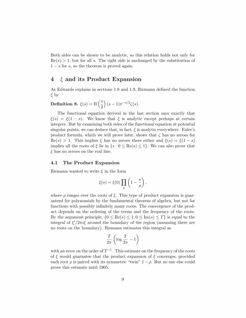
Both sides can be shown to be analytic, so this relation holds not only forRe(s) > 1, but for all s. The right side is unchanged by the substitution of1− s for s, so the theorem is proved again.

4 ξ and its Product Expansion

As Edwards explains in sections 1.8 and 1.9, Riemann defined the functionξ by

Definition 8. ξ(s) = Π(s

2

)(s− 1)π−s/2ζ(s).

The functional equation derived in the last section says exactly thatξ(s) = ξ(1 − s). We know that ξ is analytic except perhaps at certainintegers. But by examining both sides of the functional equation at potentialsingular points, we can deduce that, in fact, ξ is analytic everywhere. Euler’sproduct formula, which we will prove later, shows that ζ has no zeroes forRe(s) > 1. This implies ξ has no zeroes there either and ξ(s) = ξ(1 − s)implies all the roots of ξ lie in {s : 0 ≤ Re(s) ≤ 1}. We can also prove thatξ has no zeroes on the real line.

4.1 The Product Expansion

Riemann wanted to write ξ in the form

ξ(s) = ξ(0)∏ρ

(1− s

ρ

),

where ρ ranges over the roots of ξ. This type of product expansion is guar-anteed for polynomials by the fundamental theorem of algebra, but not forfunctions with possibly infinitely many roots. The convergence of the prod-uct depends on the ordering of the terms and the frequency of the roots.By the argument principle, {0 ≤ Re(s) ≤ 1, 0 ≤ Im(s) ≤ T} is equal to theintegral of ξ′/2πiξ around the boundary of the region (assuming there areno roots on the boundary). Riemann estimates this integral as

T

2π

(log

T

2π− 1

)with an error on the order of T−1. This estimate on the frequency of the rootsof ξ would guarantee that the product expansion of ξ converges, providedeach root ρ is paired with its symmetric “twin” 1−ρ. But no one else couldprove this estimate until 1905.

9

4.2 Proof by Hadamard’s Theorem

Hadamard proved that the product representation of ξ was valid in 1893.His methods gave rise to a more general result, the Hadamard factorizationtheorem. Edwards devotes chapter 2 to Hadamard’s proof of the productformula for ξ. But for the sake of space I will simply quote Hadamard’stheorem to justify that formula. The reader may consult Taylor chapter8 for a succinct development of the general theorem, which I merely statehere, as given in [2]:

Theorem 9 (Hadamard’s Factorization Theorem). Suppose f is entire. Letp be an integer and suppose there exists positive t < p+ 1 such that |f(z)| ≤exp(|z|t) for z sufficiently large. Then f can be factored as

f(z) = zmeh(z)∞∏k=1

Ep

(z

zk

),

where {zk} is a list of the roots of f counting multiplicity, m is the order ofthe zero of f at 0, h(z) is a polynomial of degree at most p, and Ep(w) =(1− w) exp(

∑pn=1w

n/n).

To apply the theorem, we must estimate ξ. To do this we need Riemann’salternate representation of ξ based on the result of the previous section

ξ(s) =1

2− s(1− s)

2

∫ ∞1

φ(x)(xs/2 + x1/2−s/2)dx

x,

which Edwards derives in section 1.8. Using more integration by parts andchange of variables, we can show that

ξ(s) = 4

∫ ∞1

d

dx

[x3/2φ′(x)

]x−1/4 cosh

(12(s− 1

2) log x)dx.

Substituting the power series for coshw =∑∞

n=0wn/(2n)! will show that

the power series for ξ(s) about s = 12 has coefficients

a2n =4

(2n)!

∫ ∞1

d

dx

[x3/2φ′(x)

]x−1/4(12 log x)2n dx.

Direct evaluation of (d/dx)[x3/2φ′(x)] will show that the integrand is posi-tive. Hence, ξ has a power series about 1

2 with real, positive coefficients.This is all we need to derive a “simple estimate” of ξ as Edwards does

in section 2.3:

10

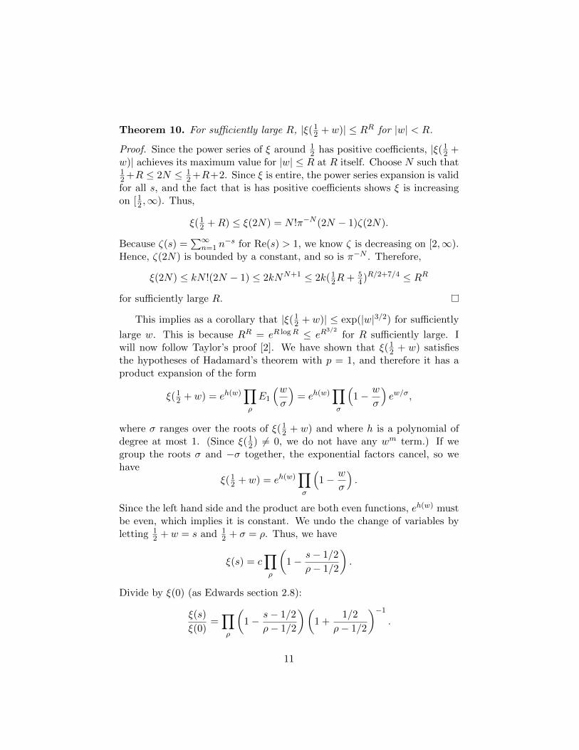
Theorem 10. For sufficiently large R, |ξ(12 + w)| ≤ RR for |w| < R.

Proof. Since the power series of ξ around 12 has positive coefficients, |ξ(12 +

w)| achieves its maximum value for |w| ≤ R at R itself. Choose N such that12 +R ≤ 2N ≤ 1

2 +R+2. Since ξ is entire, the power series expansion is validfor all s, and the fact that is has positive coefficients shows ξ is increasingon [12 ,∞). Thus,

ξ(12 +R) ≤ ξ(2N) = N !π−N (2N − 1)ζ(2N).

Because ζ(s) =∑∞

n=1 n−s for Re(s) > 1, we know ζ is decreasing on [2,∞).

Hence, ζ(2N) is bounded by a constant, and so is π−N . Therefore,

ξ(2N) ≤ kN !(2N − 1) ≤ 2kNN+1 ≤ 2k(12R+ 54)R/2+7/4 ≤ RR

for sufficiently large R.

This implies as a corollary that |ξ(12 + w)| ≤ exp(|w|3/2) for sufficiently

large w. This is because RR = eR logR ≤ eR3/2

for R sufficiently large. Iwill now follow Taylor’s proof [2]. We have shown that ξ(12 + w) satisfiesthe hypotheses of Hadamard’s theorem with p = 1, and therefore it has aproduct expansion of the form

ξ(12 + w) = eh(w)∏ρ

E1

(wσ

)= eh(w)

∏σ

(1− w

σ

)ew/σ,

where σ ranges over the roots of ξ(12 + w) and where h is a polynomial ofdegree at most 1. (Since ξ(12) 6= 0, we do not have any wm term.) If wegroup the roots σ and −σ together, the exponential factors cancel, so wehave

ξ(12 + w) = eh(w)∏σ

(1− w

σ

).

Since the left hand side and the product are both even functions, eh(w) mustbe even, which implies it is constant. We undo the change of variables byletting 1

2 + w = s and 12 + σ = ρ. Thus, we have

ξ(s) = c∏ρ

(1− s− 1/2

ρ− 1/2

).

Divide by ξ(0) (as Edwards section 2.8):

ξ(s)

ξ(0)=∏ρ

(1− s− 1/2

ρ− 1/2

)(1 +

1/2

ρ− 1/2

)−1.

11

Each term in the product is a linear function of s which is 0 when s = ρ and1 when s = 0. Hence, each term is 1− s/ρ and we have

Theorem 11. ξ has a product expansion

ξ(s) = ξ(0)∏ρ

(1− s

ρ

),

where ρ ranges over the roots of ξ, and ρ and 1− ρ are paired.

5 Zeta and Primes: Euler’s Product Formula

The zeta function is connected to prime numbers by

Theorem 12. For Re(s) > 1,

ζ(s) =∏p

(1− p−s)−1,

where p ranges over the prime numbers.

This identity is derived from the Dirichlet series in the following way.Edwards does not give the proof, but for the sake of completeness I includea proof adapted from Taylor [2].

Proof. Let pn be the nth prime number. Define sets SN and TN inductivelyas follows. Let S0 be the positive integers. For N ≥ 0, let TN+1 be the set ofnumbers in SN divisible by PN and let SN+1 = SN \ TN+1. Notice that SNis the set of positive integers not divisible by the first N primes, and TN+1

exactly {pN+1m : m ∈ SN}. I will show by induction that for Re(s) > 1,

ζ(s)N∏n=1

(1− 1

psn

)=∑n∈SN

1

ns.

Since S0 = Z+, we have ζ(s) =∑

n∈S0n−s. Now suppose the statement

holds for N . Multiply by (1− p−sN+1):

ζ(s)N+1∏n=1

(1− 1

psn

)=

(1− 1

psN+1

) ∑n∈SN

1

ns

=∑n∈SN

1

ns−∑n∈SN

1

(PN+1n)s

=∑n∈SN

1

ns−

∑n∈TN+1

1

ns=

∑n∈SN+1

1

ns,

12

where the last equality holds because SN \ TN+1 = SN+1 and TN+1 ⊂ SN .This completes the induction.

The proof will be complete if we show that∑

n∈SN n−s approaches 1 as

N →∞. Notice that if 1 < n ≤ N < PN , then n 6∈ SN . This is because anyprime factor of n has to be less than or equal to PN , but all multiples of allprimes pn ≤ PN have been removed from SN . Hence,∣∣∣∣∣ ∑

n∈SN

1

ns− 1

∣∣∣∣∣ =

∣∣∣∣∣ ∑N≤n∈SN

1

ns

∣∣∣∣∣ ≤ ∑N≤n∈SN

∣∣∣∣ 1

ns

∣∣∣∣ ≤ ∞∑n=N

∣∣∣∣ 1

ns

∣∣∣∣ .We are justified in applying the triangle inequality here because the right-most sum converges absolutely. Indeed, the sum on the right is smaller thanany positive ε for N sufficiently large. Hence, the limit of

∑n∈SN n

−s is1.

Taking the log of this formula gives log ζ(s) = −∑

p log(1 − p−s) forRe(s) > 1. Since log(1− x) = −

∑∞n=1 x

n/n, we have

log ζ(s) =∑p

∞∑n=1

1

np−sn.

There is a problem in that log z is only defined up to multiples of 2πi.However, it is easy to make the statement rigorous. We simply say that theright hand side provides one logarithm for ζ. We can also argue that it isanalytic.

6 Riemann’s Main Formula: Summary

Riemann uses the formula for log ζ(s) to evaluate J(x), a function whichmeasures primes. Since I am going to prove Von Mangoldt’s similar formulalater, I will only sketch Riemann’s methods here. J(x) is a step functionwhich starts at J(0) = 0 and jumps up at positive integers. The jump is1 at primes, 1

2 at squares of primes, 13 at cubes of primes, etc. J can be

written as

J(x) =∑p

∞∑n=1

1

nu(x− pn),

where u(x) = 0 for x < 0, u(0) = 12 , and u(x) = 1 for x > 0. We can obtain

a formula for π(x), the number of primes less than x from J(x).

13

Since J(x) ≤ x and J(x) = 0 for x < 2, we know that for Re(s) > 1,∫∞0 J(x)x−s−1 dx converges. Hence, by Theorem 4, we can integrate term

by term and∫ ∞0

J(x)x−s−1 dx =∑p

∞∑n=1

1

n

∫ ∞pn

x−s−1 dx =1

s

∑p

∞∑n=1

1

np−sn,

which is s−1 log ζ(s).Through a change of variables and Fourier inversion, Riemann recovers

J(x) from the integral formula:

J(x) =1

2πi

∫ a+i∞

a−i∞(log ζ(s))xs

ds

s,

where a > 1 and the integral is defined as the Cauchy principal value

limT→+∞

∫ a+iT

a−iT(log ζ(s))xs

ds

s,

He then integrates by parts and shows the first term goes to zero to obtain:

J(x) = − 1

2πi

∫ a+i∞

a−i∞

d

ds

[log ζ(s)

s

]xs ds.

Applying ξ(s) = Π(s/2)(s − 1)π−s/2ζ(s) together with the product for-mula for ξ gives:

log ζ(s) = log ξ(s) +s

2log π − log(s− 1)− log Π

(s2

)= log ξ(0) +

∑ρ

log

(1− s

ρ

)+s

2log π − log(s− 1)− log Π

(s2

).

He substitutes this into the integral for J(x), then evaluates the integralterm by term as

J(x) = Li(x)−∑

Imρ>0

[Li(xρ) + Li(x1−ρ)] +

∫ ∞x

dt

t(t2 − 1) log t+ log ξ(0),

where Li(x) is the Cauchy principal value of∫ x0 1/ log x dx. The evaluation

requires too much work to explain it completely here (Edwards sections1.13-1.16), but the term-by-term integration itself is even more difficult tojustify, and Riemann’s main formula was not proved until Von Mangoldt’swork in 1905.

14

7 Von Mangoldt’s Formula

Von Mangoldt’s formula is essentially the same as Riemann’s, except thatinstead of considering log ζ(s), he considers its derivative ζ ′(s)/ζ(s). Bydifferentiating the formula for log ζ(s) as a sum over primes, we have

ζ ′(s)

ζ(s)= −

∑p

∞∑n=1

p−ns log p, Re(s) > 1.

Instead of J(x), we use a different step function ψ(x) defined by

ψ(x) =∑p

∞∑n=1

(log p)u(x− pn).

Van Mangoldt shows that

ψ(x) = x−∑ρ

xρ

ρ+

∞∑n=1

x−2n

2n− ζ ′(0)

ζ(0),

by showing that both sides are equal to

− 1

2πi

∫ a+i∞

a−i∞

ζ ′(s)

ζ(s)xsds

s.

(In the sum over ρ, we pair ρ with 1−ρ and sum in order of increasing Im(ρ).In the integral from a− i∞ to a+ i∞ we take the Cauchy principal value.)His proof, like Riemann’s, depends on several tricky termwise integrations.

7.1 First Evaluation of the Integral

First, we show that the integral is equal to ψ(x). We let Λ(m) be the sizeof the jump of ψ at m; it is log p if m = pn and zero otherwise. We thenrewrite the series for ζ ′/ζ and ψ as

ζ ′(s)

ζ(s)= −

∞∑m=1

Λ(m)m−s, ψ(x) =

∞∑m=1

Λ(m)u(x−m).

The rearrangement is justified because the series converge absolutely. Wethen have

− 1

2πi

∫ a+i∞

a−i∞

ζ ′(s)

ζ(s)xsds

s=

1

2πi

∫ a+i∞

a−i∞

( ∞∑m=1

Λ(m)xs

ms

)ds

s.

15

We want to integrate term by term. This is justifiable on a finite intervalbecause the series converges uniformly for Re(s) ≥ a > 1 (since Λ(m) ≤logm and x is constant). Thus, we have

1

2πi

∫ a+ih

a−ih

( ∞∑m=1

Λ(m)xs

ms

)ds

s=

1

2πi

∞∑m=1

Λ(m)

∫ a+ih

a−ih

xs

ms

ds

s.

To take the limit as h → ∞ and evaluate the integral, we will need thefollowing lemma, which can be proved by straightforward estimates andintegration by parts.

Lemma 13. For t > 0,

limh→+∞

1

2πi

∫ a+ih

a−ihtsds

s= u(t− 1) =

0 t < 112 , t = 1

1, t > 1.

For 0 < t < 1 and for 1 < t, the error∣∣∣∣ 1

2πi

∫ a+ih

a−ihtsds

s− u(t− 1)

∣∣∣∣ ≤ ta

πh| log t|.

Let x/m be the t in the lemma and noticing u(x/m− 1) = u(x−m), wehave

Λ(m)

∣∣∣∣ 1

2πi

∫ a+ih

a−ih

xs

ms

ds

s− u(x−m)

∣∣∣∣ ≤ (x/m)a logm

πh| log x− logm|

The right hand side is summable over m because (logm)/| log x − logm|approaches 1 as m→∞ and (x/m)a is summable. Thus, for fixed x,

∞∑m=1

Λ(m)

∣∣∣∣∫ a+ih

a−ih

xs

ms

ds

s− u(x−m)

∣∣∣∣ ≤ K

h,

for some constant K. Hence, the limit of the sum as h → ∞ is zero. Thisargument assumes x 6= m, but if x is an integer, we can simply throw awaythe terms where m ≤ x, since finitely many terms do not affect convergence.This implies

limh→∞

1

2πi

∞∑m=1

Λ(m)

∫ a+ih

a−ih

xs

ms

ds

s=

∞∑m=1

Λ(m)u(x−m),

or

− 1

2πi

∫ a+i∞

a−i∞

ζ ′(s)

ζ(s)xsds

s= ψ(x).

This completes the first evaluation of the integral.

16

7.2 Second Evaluation of the Integral

For the second evaluation, we use a different formula for ζ ′/ζ. Differentiate

log ζ(s) = log ξ(0) +∑ρ

log

(1− s

ρ

)+s

2log π − log(s− 1)− log Π

(s2

)to obtain

−ζ′(s)

ζ(s)=∑ρ

1

ρ− s− 1

2log π +

1

s− 1+

d

dslog Π

(s2

)In order to justify termwise differentiation, we use the fact proved by Hadamard(and which we will not prove here!) that

∑ρ 1/ρ with the roots ρ and 1− ρ

paired converges absolutely. We order the terms by increasing |Im(ρ)|. Sincelim|Im(ρ)|→∞

ρρ−s = 1, ∣∣∣∣ 1

ρ− s

∣∣∣∣ < ∣∣∣∣kρ∣∣∣∣

for any fixed s, for Im(ρ) sufficiently large. In fact, on the set {s : Re(s) >1 + δ,−a < Im(s) < a}, we can bound |1/(ρ− s)| uniformly by |1/(ρ− s0)|where s0 = 1 + δ + ai. This shows that the series converges uniformly oncompact sets and term-by-term differentiation is justified.

In the preceding formula, substitute the product formula for Π(s) =∏∞n=1(1 + s/n)−1(1 + 1/n)s from Theorem 3:

d

dslog Π

(s2

)=

d

ds

∞∑n=1

(s log

(1 +

1

2n

)− log

(1 +

s

2n

))

=∞∑n=1

(log

(1 +

1

2n

)+

1

2n+ s

)This termwise differentiation is justifiable because the differentiated seriesconverges uniformly on compact subsets of C with Re(s) > 1. The readermay verify this: Use the power series for log(1 + t) and show that each termof the differentiated series is less than a constant times 1/n2.

Using these formulae, we have

−ζ′(s)

ζ(s)+ζ ′(0)

ζ(0)=∑ρ

1

ρ− s−∑ρ

1

ρ+

1

s− 1+ 1 +

∞∑n=1

(1

2n+ s+

1

2n

)

−ζ′(s)

ζ(s)=

s

s− 1−∑ρ

s

ρ(s− ρ)+

∞∑n=1

s

2n(s+ 2n)− ζ ′(0)

ζ(0).

17

This is the formula for ζ ′/ζ we intend to integrate term by term. To do this,we need another lemma. The reader may try deducing this lemma from theprevious one using a change of variables and Cauchy’s theorem.

Lemma 14. For a > 1 and x > 1,∫ a+i∞

a−i∞

1

s− βxs ds = xβ

The lemma allows us immediately to integrate the first and last terms:

1

2πi

∫ a+i∞

a−i∞

s

s− 1xsds

s= x, − 1

2πi

∫ a+i∞

a−i∞

ζ ′(0)

ζ(0)xsds

s=ζ ′(0)

ζ(0).

The lemma also tells us what the value of other integrals will be, if we canjustify term-by-term integration.

First, consider

1

2πi

∫ a+i∞

a−i∞

( ∞∑n=1

s

2n(s+ 2n)

)xsds

s.

Because the series converges uniformly on compact subsets of {Re(s) > 1},we can integrate term by term over a finite interval. We only have to worryabout taking the limit

limh→∞

∞∑n=1

1

2πi

1

2n

∫ a+ih

a−ih

xs

s+ 2nds.

To justify the termwise limit, we begin by showing that the sum of thelimits converges. By Lemma 14,

1

2πi

1

2n

∫ a+i∞

a−i∞

xs

s+ 2nds =

x−2n

2n.

This is clearly summable over n (in fact, it sums to −12 log(1 − x−2)). We

now show that the sum before we take the limit (that is, the sum of thepartial integrals) converges, using the estimate

Lemma 15. For x > 1, a > 0, and d > c ≥ 0,∣∣∣∣ 1

2πi

∫ a+di

a+ci

ts

sds

∣∣∣∣ ≤ K

(a+ c) log t.

18

By change of variables,∫ a+ih

a−ih

xs

s+ 2nds = x−2n

∫ a+2n+ih

a+2n−ih

xs

sds = 2x−2n

∫ a+2n−ih

a+2n

xs

sds.

And by Lemma 15,∣∣∣∣2x−2n 1

2πi

∫ a+2n−ih

0

xs

sds

∣∣∣∣ ≤ 2Kx−2n

(a+ 2n) log x≤ K ′

n2.

Hence, the sum of the partial integrals is summable. This implies thatevaluating the limit termwise is valid. This is because for any ε > 0, wecan choose N large enough that the sum of the first N infinite integrals iswithin ε of the complete sum. By choosing N larger if necessary, we canmake the sum of the first N finite integrals within ε/3 of its limit, uniformlyin h. Then by choosing h large enough, we can make the first N integralsbe within ε/3N of their limits. Thus, the two partial sums are within ε/3of each other, and so the infinite sum of the infinite integrals is within ε ofthe infinite sum of the finite integrals.

All that remains is to evaluate the integral of∑

ρ s/ρ(ρ− s).

7.3 Termwise Evaluation over ρ

We will need the following lemma on the density of the roots of ξ, givenin Edwards section 3.4. The proof of this lemma is highly nontrivial. It isultimately based on Hadamard’s results.

Lemma 16. For T sufficiently large, ξ has fewer than 2 log T roots in T ≤Im(ρ) ≤ T + 1.

We want to evaluate

1

2πi

∫ a+i∞

a−i∞

(∑ρ

s

ρ(s− ρ)

)xsds

s.

We first note that we can exchange summation and integration for a finiteintegral:

limh→∞

∑ρ

1

2πi

∫ a+ih

a−ih

xs

ρ(s− ρ)ds.

Uniform convergence of the series is obtained from Hadamard’s result that∑ρ |ρ −

12 |−2 converges. After pairing the terms for ρ and 1 − ρ, we can

19

show that each term of the series is less than a constant times |ρ − 12 |−2.

The proof is merely a manipulation of fractions and is left to the reader.We already know the limit exists because we have shown that all the

other terms in von Mangoldt’s formula have limits as h→∞. Von Mangoldtconsiders the diagonal limit

limh→∞

∑|Im(ρ)|≤h

xρ

ρ

∫ a+ih

a−ih

xs−ρ

s− ρds.

He shows that∑ρ

xρ

ρ

∫ a+ih

a−ih

xs−ρ

s− ρds−

∑|Im(ρ)|≤h

xρ

ρ

∫ a+ih

a−ih

xs−ρ

s− ρds

approaches zero, so that the diagonal limit exists and is equal to the originallimit. If ρ is written as β + iγ, then we can estimate the sum of roots withpositive γ as∑

γ>h

∣∣∣∣xρρ∣∣∣∣ ∣∣∣∣ 1

2πi

∫ a+ih

a−ih

xs−ρ

s− ρds

∣∣∣∣ ≤∑γ>h

xβ

γ

∣∣∣∣∣ 1

2πi

∫ a−β+i(γ+h)

a−β+i(γ−h)

xt

tds

∣∣∣∣∣ ,This, in turn, is less than or equal to∑

γ>h

xβ

γ

Kxa−β

(a− β + γ − h) log x

by Lemma 15, which is less than or equal to

Kxa

log x

∑γ>h

1

γ

K

γ(γ − h+ c) log x,

where c = a− 1 so that 0 < c ≤ a− β. By writing the roots with γ < 0 as1− ρ = 1− β − iγ and making a change of variables, the reader may verifythat the same chain of inequalities applies with β replaced by 1−β, but thec we chose works for that case as well. Hence, the sum over all roots can beestimated by twice the above estimate.

Now take h sufficiently large that Lemma 16 applies. Arrange the rootsinto groups where h + j ≤ γ < h + j + 1 for each integer j. There are atmost 2 log(h + j) roots in each group, so summing over j makes the abovequantities smaller than a constant multiple of

∞∑j=0

log(h+ j)

(h+ j)(j + c).

20

This sum converges and as h → ∞, it approaches zero; the proof of this isleft to the reader.

We now only have to evaluate the diagonal limit, and we know that itexists. We will show that∑

|Im(ρ)|≤h

xρ

ρ

∫ a+ih

a−ih

xs−ρ

s− ρds−

∑|Im(ρ)|≤h

xρ

ρ

approaches zero as h → ∞. This will prove that∑

ρ xρ/ρ converges and

is equal to the diagonal limit. By similar reasoning as before, the abovedifference is smaller than twice∑

0<γ≤h

∣∣∣∣xρρ∣∣∣∣ ∣∣∣∣ 1

2πi

∫ a−β−iγ+ih

a−β−iγ−ih

xt

tdt− 1

∣∣∣∣ ,which is no larger than∑0<γ≤h

∣∣∣∣xρρ∣∣∣∣∣∣∣∣∣ 1

2πi

∫ a−β+i(h+γ)

a−β−i(h+γ)

xt

tdt− 1

∣∣∣∣∣+ ∑0<γ≤h

∣∣∣∣xρρ∣∣∣∣∣∣∣∣∣ 1

2πi

∫ a−β+i(h−γ)

a−β+i(h+γ)

xt

tdt

∣∣∣∣∣by path additivity of integrals and the triangle inequality. By Lemmas 13and 15 and similar manipulation as before, this is less than or equal to

∑0<γ≤h

xβ

γ

xa−β

π(h+ γ) log x+∑

0<γ≤h

xβ

γ

Kxa−β

γ(a− β + h− γ) log x

≤ xa

π log x

∑0<γ≤h

1

γ(h+ γ)+Kxa

log x

∑0<γ≤h

1

γ(c+ h− γ),

where c = a − 1. Our object is to show that this series approach zero ash→∞. We fix an H such that the estimate of Lemma 16 holds for h ≥ H.There are only finitely many terms where γ ≤ H, and it is easy to see eachterm approaches zero as h → ∞. The remaining terms we put into groupswhere h + j ≤ γ < h + j + 1 as before and apply the estimate of Lemma16. We estimate the quantity by convergent series which approach zero ash → ∞; since the argument is similar to the one we did before, I will skipthe details.

This completes the proof that

1

2πi

∫ a+i∞

a−i∞

(∑ρ

s

ρ(s− ρ)

)xsds

s= lim

h→∞

∑|Im(ρ)|≤h

xρ

ρ

∫ a+ih

a−ih

xs−ρ

s− ρds =

∑ρ

xρ

ρ.

21

7.4 Von Mangoldt’s and Riemann’s Formulae

We have now evaluated term by term

1

2πi

∫ a+i∞

a−i∞

(s

s− 1−∑ρ

s

ρ(s− ρ)+∞∑n=1

s

2n(s+ 2n)− ζ ′(0)

ζ(0)

)xsds

s,

showing that

x−∑ρ

xρ

ρ+

∞∑n=1

x−2n

2n− ζ ′(0)

ζ(0)= − 1

2πi

∫ a+i∞

a−i∞

ζ ′(s)

ζ(s)xsds

s= ψ(x).

The one thing missing from von Mangoldt’s formula is the evaluation ofζ ′(0)/ζ(0) which Edwards performs in section 3.8. It is log 2π.

Von Mangoldt used his formula to prove Riemann’s main formula; Ed-wards explains this proof in section 3.7. Von Mangoldt used a differentmethod from Riemann’s and did not directly justify Riemann’s term-by-term integration, although three years later in 1908, Landau did just that.Von Mangoldt’s formula can also be used to prove the prime number theo-rem, which says essentially that ψ(x)/x approaches 1 as x→∞.

References

[1] Harold M. Edwards. Riemann’s Zeta Function. 1974. Dover Publica-tions.

[2] Joseph L. Taylor. Complex Variables. 2011. American MathematicalSociety.

22