an introduction to the riemann zeta function content …michel.waldschmidt/articles/pdf/zeta... ·...
TRANSCRIPT
Artin L–functions, Artin primitive roots Conjecture and applications
CIMPA-ICTP Research School, Nesin Mathematics Village 2017
An introduction to the Riemann zeta function
Michel Waldschmidt
Content of this file (29 pages).
• p.2–3: a list of references.
• p. 4–22: from the book Arithmetics by M. Hindry: p. 127–131, 134–139,
148–155.
• p. 23–29: from ´
Elements d’analyse et d’algebre (et de theorie des nom-
bres) by P. Colmez : p. 40–43 and 51–53.
Further main references (not included in this file):
• Lectures on the Riemann zeta function by H. Iwaniec, Chap. 1–12, p.
3–43.
• An introduction to the theory of the Riemann zeta-function by S. J. Pat-
terson, Chap. 1–11, p. 1–66.
• An introduction to zeta functions by P. Cartier, p 1–63.
1
References
LMFDB is the database of L-functions, modular forms, and related objects. It
is an extensive database of mathematical objects arising in Number Theory.
http://www.lmfdb.org/
A basic course in number theory, containing the basic elements of analytic num-
ber theory, is
• M. Hindry, Arithmetics, Universitext, Springer, London, 2011. Trans-
lated from the 2008 French original.
Perhaps the simplest and more direct introduction to the Riemann zeta function
is contained in the recent small (and a bit synthetic) book :
• H. Iwaniec, Lectures on the Riemann zeta function, vol. 62 of University
Lecture Series, American Mathematical Society, Providence, RI, 2014.
Chapters 5–7 (p.21–26) present the theory from the beginning to the functional
equation; chapters 8–11 (p.27–42) contain the rest of the basic theory, ending
with the proof of PNT.
A discussion of the special values of the Riemann zeta function is included in
• P. Cartier, An introduction to zeta functions, in From number theory
to physics (Les Houches, 1989), Springer, Berlin, 1992, pp. 1–63.
One of the most classical reference is
• G. H. Hardy and E. M. Wright, An introduction to the theory of
numbers, Oxford University Press, Oxford, sixth ed., 2008. Revised by D.
R. Heath-Brown and J. H. Silverman, With a foreword by Andrew Wiles.
Other classical books, all containing the basic theory of ⇣(s), are:
• A. E. Ingham, The distribution of prime numbers, Cambridge Mathe-
matical Library, Cambridge University Press, Cambridge, 1990. Reprint
of the 1932 original, With a foreword by R. C. Vaughan.
2
• E. C. Titchmarsh, The theory of the Riemann zeta-function, The Claren-
don Press, Oxford University Press, New York, second ed., 1986. Edited
and with a preface by D. R. Heath-Brown.
• T. M. Apostol, Introduction to analytic number theory, Springer-Verlag,
New York-Heidelberg, 1976. Undergraduate Texts in Mathematics.
• A. A. Karatsuba, Basic analytic number theory, Springer-Verlag, Berlin,
1993. Translated from the second (1983) Russian edition and with a
preface by Melvyn B. Nathanson.
• S. J. Patterson, An introduction to the theory of the Riemann zeta-
function, vol. 14 of Cambridge Studies in Advanced Mathematics, Cam-
bridge University Press, Cambridge, 1988.
• H. Davenport, Multiplicative number theory, vol. 74 of Graduate Texts
in Mathematics, Springer-Verlag, New York, third ed., 2000. Revised and
with a preface by Hugh L. Montgomery.
• H. L. Montgomery and R. C. Vaughan, Multiplicative number theory.
I. Classical theory, vol. 97 of Cambridge Studies in Advanced Mathemat-
ics, Cambridge University Press, Cambridge, 2007.
• G. Tenenbaum, Introduction to analytic and probabilistic number theory,
vol. 163 of Graduate Studies in Mathematics, American Mathematical
Society, Providence, RI, third ed., 2015. Translated from the 2008 French
edition by Patrick D. F. Ion.
• P. Colmez, ´
Elements d’analyse et d’algebre (et de theorie des nombres),
les editions de l’ecole polytechnique, 2011, 678 pages.
3

§1. Elementary Statements and Estimates 127
1.6. Theorem. As x tends to infinity, we have the following asymptoticbehavior:
π(x; a, b) := card{p prime , p ! x, p ≡ a mod b} ∼ xφ(b) log x
· (4.4)
In this section, we will expand on some so-called “elementary” methods(which in this context means that they do not involve complex variables)which can be used to prove the previous assertions, except for Dirichlet’stheorem on arithmetic progressions and the prime number theorem. Theywill however allow us to prove a partial version: there exist two constants,c1, c2 > 0, such that c1x/ log x ! π(x) ! c2x/ log x.
1.7. Lemma. The following estimate holds: n log 2 ! log(2n
n
)! n log 4.
Proof. From the binomial theorem, we know that(2n
n
)! ∑2n
k=0
(2nk
)=
(1+1)2n = 4n. Next, we have the following lower bound:(
2n
n
)=
(2n)!(n!)2
=
2n(2n − 1) · · · (n + 1)n(n − 1) · · · 1
" 2n. #
1.8. Lemma. The following formula holds: ordp(n!) =∑
m!1
⌊npm
⌋;
furthermore, the sum can be restricted to m ! log n/ log p.
Proof. Write n! =1 ·2 ·3 · · ·n =∏n
k=1 k. The number of integers ! n whichare divisible by p is ⌊n/p⌋, and the number of integers ! n divisible by p2
is ⌊n/p2⌋, etc. Thus ordp(n!) is the sum of the ⌊n/pm⌋. Finally, pm ! n isequivalent to m ! log n/ log p, hence the first statement is proved. #
We can therefore write
log(
2n
n
)=
∑
p"2n
ordp
(2n
n
)log p =
∑
p"2n
⎛
⎝∑
m!1
⌊2npm
⌋− 2
⌊npm
⌋⎞
⎠ log p.
(4.5)To find a lower bound, we only keep the terms that satisfy n < p ! 2n. Infact, such a p clearly divides
(2nn
)= (2n)!/(n!)2, and thus we obtain
n log 4 " log(
2n
n
)"
∑
n<p"2n
log p = θ(2n) − θ(n).
From this, we obtain an upper bound of the form θ(x) ! Cx. This is truebecause
128 4. Analytic Number Theory
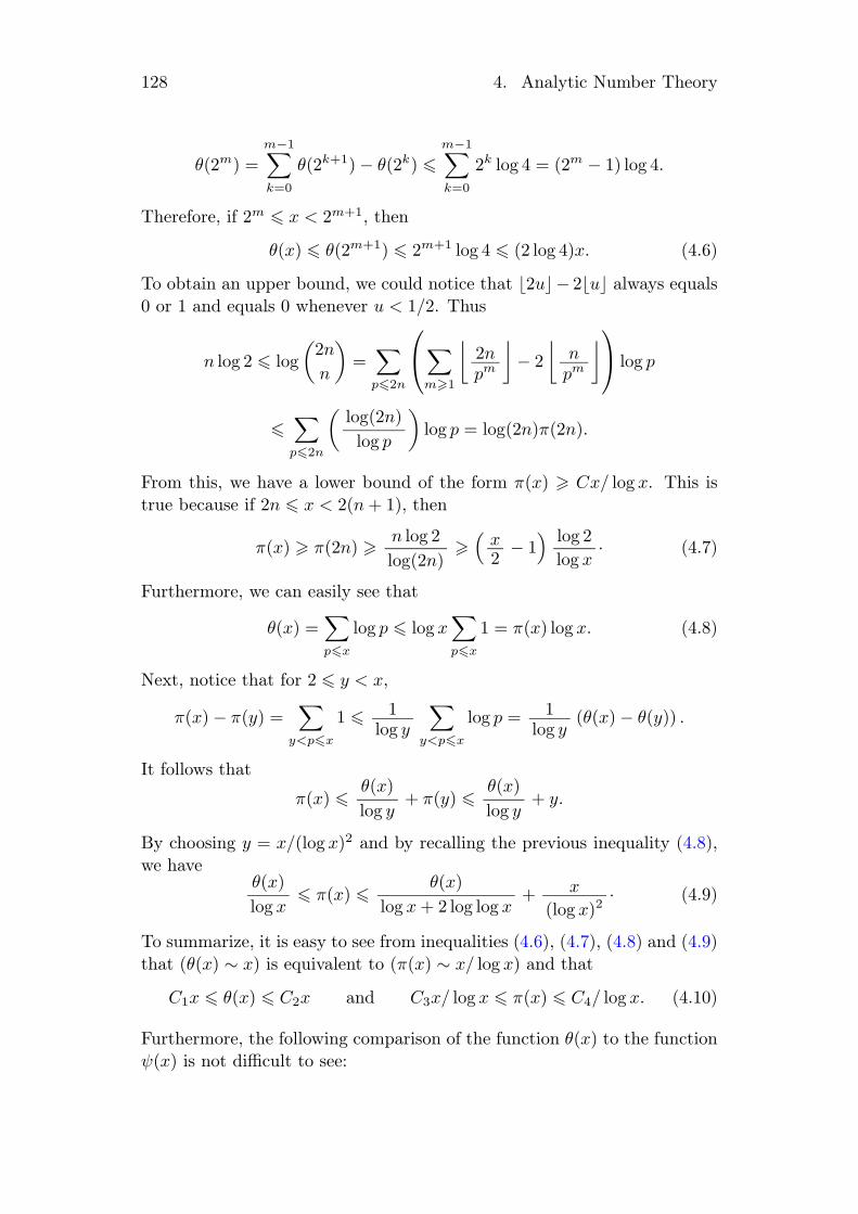
θ(2m) =m−1∑
k=0
θ(2k+1) − θ(2k) !m−1∑
k=0
2k log 4 = (2m − 1) log 4.
Therefore, if 2m ! x < 2m+1, then
θ(x) ! θ(2m+1) ! 2m+1 log 4 ! (2 log 4)x. (4.6)
To obtain an upper bound, we could notice that ⌊2u⌋− 2⌊u⌋ always equals0 or 1 and equals 0 whenever u < 1/2. Thus
n log 2 ! log(
2n
n
)=
∑
p"2n
⎛
⎝∑
m!1
⌊2npm
⌋− 2
⌊npm
⌋⎞
⎠ log p
!∑
p"2n
(log(2n)log p
)log p = log(2n)π(2n).
From this, we have a lower bound of the form π(x) " Cx/ log x. This istrue because if 2n ! x < 2(n + 1), then
π(x) " π(2n) " n log 2log(2n)
"(
x2 − 1
) log 2log x
· (4.7)
Furthermore, we can easily see that
θ(x) =∑
p"x
log p ! log x∑
p"x
1 = π(x) log x. (4.8)
Next, notice that for 2 ! y < x,
π(x) − π(y) =∑
y<p"x
1 ! 1log y
∑
y<p"x
log p = 1log y
(θ(x) − θ(y)) .
It follows thatπ(x) ! θ(x)
log y+ π(y) ! θ(x)
log y+ y.
By choosing y = x/(log x)2 and by recalling the previous inequality (4.8),we have
θ(x)log x
! π(x) ! θ(x)log x + 2 log log x
+ x(log x)2
· (4.9)
To summarize, it is easy to see from inequalities (4.6), (4.7), (4.8) and (4.9)that (θ(x) ∼ x) is equivalent to (π(x) ∼ x/ log x) and that
C1x ! θ(x) ! C2x and C3x/ log x ! π(x) ! C4/ log x. (4.10)
Furthermore, the following comparison of the function θ(x) to the functionψ(x) is not difficult to see:

§1. Elementary Statements and Estimates 129
θ(x) ! ψ(x) :=∑
pm"x
log p = θ(x) + θ(√
x) + θ( 3√
x) + . . .
! θ(x) +log(x)log 2
θ(√
x) ! θ(x) + C log x√
x.
Finally, if we denote by pn the nth prime number, we have π(pn) = n by def-inition. The prime number theorem therefore implies that n ∼ pn/ log(pn)and that pn ∼ n log n. We can check that the latter statement is in factequivalent to the prime number theorem.
1.9. Lemma. (Abel’s formula) Let A(x) :=∑
n"x an and f be a functionof class C 1. Then,
∑
y<n"x
anf(n) = A(x)f(x) − A(y)f(y) −∫ x
yA(t)f ′(t)dt. (4.11)
Proof. We first point out that∫ n+1
n A(t)f ′(t)dt = A(n)∫ n+1
n f ′(t)dt =A(n) (f(n + 1) − f(n)). Therefore, setting N = ⌊x⌋ and M = ⌊y⌋ yields∫ N
MA(t)f ′(t)dt =
N−1∑
n=M
∫ n+1
nA(t)f ′(t)dt =
N−1∑
n=M
A(n + 1) (f(n) − f(n))
=N∑
n=M+1
f(n)(A(n − 1) − A(n)) + f(N)A(N) − A(M)f(M)
= −N∑
n=M+1
f(n)an + f(N)A(N) − A(M)f(M).
This proves the formula when x and y are integers. For the general formula,observe that∫ x
⌊x⌋A(t)f ′(t)dt = A(⌊x⌋) (f(x) − f(⌊x⌋)) = A(x)f(x) − A(⌊x⌋)f(⌊x⌋).#
Applications. 1) The formula gives a fairly precise comparison betweenthe “sum” and the “integral” (see Exercise 4-6.10 for some refinements). Tobe more precise, if we take an = 1 and integrate by parts, we have:
N∑
n=M+1
f(n) =∫ N
Mf(t)dt +
∫ N
M(t − ⌊t⌋)f ′(t)dt. (4.12)
If we choose f(t) = 1/t, we obtain
130 4. Analytic Number Theory
N∑
n=1
1n = 1 +
∫ N
1
dtt
−∫ N
1(t − ⌊t⌋) dt
t2
= log N +(
1 −∫ ∞
1(t − ⌊t⌋) dt
t2
)+
∫ ∞
N(t − ⌊t⌋) dt
t2
= log N + γ + O(
1N
),
where γ := 1 −∫ ∞1 (t − ⌊t⌋) dt
t2is Euler’s constant.
2) Take an = 1, so A(t) = ⌊t⌋, y = 1 and f(t) = log t. We therefore have
log (⌊x⌋!) = ⌊x⌋ log(x) −∫ x
1
⌊t⌋dtt
= x log x −∫ x
1dt + (⌊x⌋ − x) log x −
∫ x
1
⌊t⌋ − tt
dt
= x log x − x + O(log x).
We should point out that Stirling’s formula gives a slightly more precisestatement, namely n! ∼ nne−n
√2πn, and hence log(n!) = n log n − n +
12 log n + 1
2 log(2π) + ϵ(n) where limn→∞ ϵ(n) = 0.
Furthermore, we see that
log (⌊x⌋!) =∑
p"x
ordp (⌊x⌋!) log p
=∑
p"x
∑
m!1
⌊x
pm
⌋log p
= x∑
p"x
log pp +
∑
p"x
log p(⌊
xp
⌋− x
p
)+
∑
p"x
∑
m!2
⌊x
pm
⌋log p
= x∑
p"x
log pp + O(x),
where the last estimate comes from the upper bound θ(x) =∑
p"x log p =O(x), from (4.6) and the estimate
∑
p"x
∑
m!2
⌊x
pm
⌋log p ! x
∑
p"x
∑
m!2
log p
pm = x∑
p"x
log p
p(p − 1)= O(x).
From this, we can deduce the first formula in Proposition 4-1.2,∑
p"x
log pp = log x + O(1). (4.13)
§2. Holomorphic Functions (Summary/Reminders) 131
To get the second, we apply Abel’s formula (Lemma 4-1.9) letting f(t) =1/ log t and an = log p/p if n = p is prime and an = 0 otherwise. By setting
A(x) =∑
p"x
log pp , we have that
∑
p"x
1p =
∑
n"x
anf(n)
=A(x)log x
+∫ x
2
A(t)dt
t(log t)2
= 1 + O(1/ log x) +∫ x
2
dtt log t
+∫ x
2
(A(t) − log t)t(log t)2
dt
= log log x − log log 2 + 1 +∫ ∞
2
(A(t) − log t)t(log t)2
dt + O(1/ log x).
2. Holomorphic Functions(Summary/Reminders)
This section, without proofs, is a summary of some of the fundamentalproperties of functions of a complex variable that we will be using. It couldbe helpful to use [74] as a reference.Concerning series, we will use the product rule for calculating the productof two absolutely convergent series:
( ∞∑
n=0
an
)( ∞∑
n=0
bn
)=
∞∑
n=0
(n∑
k=0
akbn−k
),
as well as rearrangement of the order of summation in a series with positiveterms am,n:
∞∑
n=0
( ∞∑
m=0
am,n
)=
∞∑
m=0
( ∞∑
n=0
am,n
).
A power series S(z) =∑∞
n=0 anzn is said to have a radius of convergenceR " 0 (possibly R = 0 or R = +∞) if the series converges for all |z| < Rand diverges for all |z| > R; furthermore, the convergence is absolute inthe interior of the disc of convergence and the function is of class C∞ withS(k)(z) =
∑∞n=k n(n− 1) · · · (n− k + 1)anzn−k. In fact, the function S can
be expanded as a power series around every point z0 ∈ D(0, R), in otherwords, for every z ∈ D(z0, r) ⊂ D(0, R), we have S(z) =
∑∞n=0 bn(z − z0)n
(with bn = S(n)(z0)/n!). Such a function only has a finite number ofzeros in every closed disc (or compact set) which is contained in D(0, R).We define the multiplicity of a zero, z0, as the integer k such that S(z) =
134 4. Analytic Number Theory
The series converges normally at every point in the open disk D(1, 1) ={z ∈ C | |1 − z| < 1}, and the convergence is uniform (and also normal)on every closed disk with center 1 and radius r < 1. Therefore, F (z) isholomorphic on D(1, 1). If z is a real number in the interval ]0, 2[, we cansee that F (z) = log z (ordinary logarithm), and in particular,
exp (F (z)) = z.
The previous formula indicates that the two functions, the identity andexp ◦F , which are analytic on the disk D(1, 1), coincide on the segment]0, 2[ and hence on the whole disk. Thus F defines a complex logarithm onthe disk |z − 1| < 1.
2.8. Definition. Let f(z) be a holomorphic function on U . We saythat F (z) is a branch of the logarithm of f on U (and we write, with aslight abuse of notation, F (z) = log f(z)) if F (z) is holomorphic and ifexp (F (z)) = f(z).
2.9. Remark. If F (z) is a branch of the logarithm of f , then f is never0 on U , we have |exp (F (z))| = exp (Re F (z)) = |f(z)|, and hence
Re log f(z) = log |f(z)|.
Likewise, f ′(z)/f(z) = F ′(z) exp (F (z)) / exp (F (z)) = F ′(z), and also
ddz
log f(z) =f ′(z)f(z)
·
Finally, if F1 and F2 are two logarithms, then F2(z) = F1(z)+2kπi on anyconnected set U .
This remark suggests that we should construct the logarithm of f(z) as anantiderivative f ′(z)/f(z), with the condition that f is not zero. We haveseen that this is possible if U is simply connected.
2.10. Proposition. Let U be a simply connected open subset of thecomplex plane and f(s) a holomorphic function without any zeros in U .Then there exists a holomorphic branch F (s) = log f(s) on U . Two suchbranches differ by an integer multiple of 2πi.
We will finish this summary by explaining the notion of an infinite prod-uct. The first idea consists of saying that a product is convergent iflimN
∏Nn=0 pn exists. This could be confusing because it is not true that
such a product is zero if and only if one of the factors is zero. For example,it can be easily checked that
§3. Dirichlet Series and the Function ζ(s) 135
limN→∞
N∏
n=1
(1 − 1
n + 1
)= 0.
We can overcome this inconvenience by defining infinite products a littledifferently. Observe first that a necessary condition for the convergenceof a non-zero product
∏n pn is to have limn pn = 1; it therefore does not
hurt to assume that pn = 1 + un where un tends to zero. In particular,log(1 + un) =
∑∞k=1(−1)kuk
n/k is well-defined when |un| < 1 and hencewhen n ! n0, which justifies the following definition.
2.11. Definition. A product∏∞
n=0(1+un) is convergent (resp. absolutelyconvergent) if there exists n0 such that |un| < 1 for all n ! n0 and theseries
∑∞n=n0
log(1 + un) is convergent (resp. absolutely convergent). Aproduct of functions
∏∞n=0(1+un(z)) is uniformly convergent on K if there
exists n0 such that |un(z)| < 1 for all n ! n0 and z ∈ K and the series∑∞n=n0
log(1 + un(z)) is uniformly convergent (on K).
2.12. Lemma. A product P :=∏∞
n=0(1 + un) is absolutely convergentif and only if the series
∑∞n=0 |un| is convergent. If P is convergent, it is
zero if and only if one of the factors 1 + un is zero.
2.13. Proposition. Let (un(z)) be a sequence of holomorphic functionson an open set U such that the series
∑n log(1+un(z)) converges uniformly
on every compact subset of U .
i) Then the function defined by the infinite product
P (z) :=∞∏
n=0
(1 + un(z))
is holomorphic on U .ii) For every z0 ∈ U , only a finite number of pn(z) := 1 + un(z) are zero
at z0, and hence
ordz0 P (z) =∞∑
n=0
ordz0 pn(z).
3. Dirichlet Series and the Function ζ(s)
We call a Dirichlet series a series of the form F (s) =∑∞
n=1an
ns · We willnow state its first important property.

136 4. Analytic Number Theory
3.1. Proposition. Let F (s) =∑∞
n=1an
ns be a Dirichlet series that wewill assume to be convergent at s0. Then it converges uniformly on the setsEC,s0 = {s ∈ C | Re(s − s0) ! 0, |s − s0| " C Re(s − s0)}.
Proof. For M ! 1, set AM (x) :=∑
M<n!x ann−s0 . By the hypothesis,we then have |AM (x)| " ϵ(M) where ϵ(M) tends to zero as M tends toinfinity. Abel’s formula gives
∑
M<n!N
ann−s =∑
M<n!N
ann−s0n−(s−s0)
= AM (N)N−(s−s0) + (s − s0)∫ N
MAM (t)t−(s−s0+1)dt.
We can find an upper bound for the integral as follows:∣∣∣∣∣
∫ N
MAM (t)t−(s−s0+1)dt
∣∣∣∣∣ " ϵ(M)∫ N
Mt−(σ−σ0+1)dt
= ϵ(M) M−(σ−σ0) − N−(σ−σ0)
(σ − σ0)·
By restricting to an angular sector EC,s0 bounded by σ − σ0 = Re(s) −Re(s0) ! 0 and |s − s0| = C(σ − σ0), we obtain
∣∣∣∣∣∣
∑
M<n!N
ann−s
∣∣∣∣∣∣" ϵ(M)(1 + C),
which suffices to show the uniform convergence on this sector (cf. the figurebelow). #
the domain |s − s0| " σ − σ0
cos θ
The following corollary is a result of the general theorems recalled in theprevious section (in particular, Proposition 4-2.6).
3.2. Corollary. Every Dirichlet series F (s) =∑∞
n=1an
ns has an abscissaof convergence, say σ0, such that the series converges for Re(s) > σ0 and
§3. Dirichlet Series and the Function ζ(s) 137
diverges for Re(s) < σ0. Furthermore, the function F defined by the se-ries is holomorphic in the half-plane of convergence Re(s) > σ0, and itsderivatives are given by F (k)(s) =
∑∞n=1 an(− log n)kn−s.
Proof. It suffices to let σ0 = inf{σ ∈ R | the series converges at σ}, thento observe that every compact set in the (open) half-plane of convergenceis contained in a sector, as above, where the convergence is uniform. #
3.3. Remarks. 1) If a Dirichlet series converges at s0 = σ0 + it0 tothe number S, then the proof of Proposition 4-3.1 (above) shows thatS = limϵ→0+ F (σ0 + ϵ + it0).2) Set A(t) :=
∑n!t an. The previous proof allows us to establish the
formula∞∑
n=1
ann−s = s
∫ ∞
1
⎛
⎝∑
n!t
an
⎞
⎠ t−s−1dt = s
∫ ∞
1A(t)t−s−1dt. (4.14)
In particular, if A(t) =∑
n!t an is bounded, then the series convergeswhenever Re(s) > 0.
The most famous Dirichlet series is the Riemann zeta function, definedby the series
∑∞n=1 n−s. It is well-known, at least for real values and the
general case follows from the real case, that the abscissa of convergence is+1.
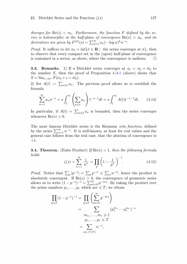
3.4. Theorem. (Euler Product) If Re(s) > 1, then the following formulaholds
ζ(s) =∞∑
n=1
1ns =
∏
p
(1 − 1
ps
)−1
. (4.15)
Proof. Notice that∑
p |p−s| =∑
p p−σ " ∑n n−σ, hence the product is
absolutely convergent. If Re(s) > 0, the convergence of geometric seriesallows us to write (1 − p−s)−1 =
∑∞m=0 p−ms. By taking the product over
the prime numbers p1, . . . , pr which are " T , we obtain
∏
p!T
(1 − p−s)−1 =∏
p!T
( ∞∑
m=0
p−ms
)
=∑
m1, . . . , mr ! 1p1, . . . , pr " T
(pm11 · · · pmr
r )−s
=∑
n∈N (T )
n−s,
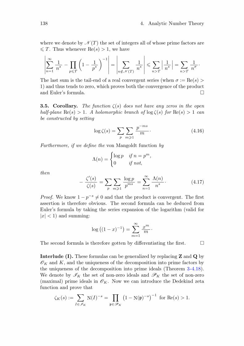
138 4. Analytic Number Theory
where we denote by N (T ) the set of integers all of whose prime factors are" T . Thus whenever Re(s) > 1, we have
∣∣∣∣∣∣
∞∑
n=1
1ns −
∏
p!T
(1 − 1
ps
)−1∣∣∣∣∣∣=
∣∣∣∣∣∣
∑
n/∈N (T )
1ns
∣∣∣∣∣∣"
∑
n>T
∣∣∣ 1ns
∣∣∣ =∑
n>T
1nσ ·
The last sum is the tail-end of a real convergent series (when σ := Re(s) >1) and thus tends to zero, which proves both the convergence of the productand Euler’s formula. #
3.5. Corollary. The function ζ(s) does not have any zeros in the openhalf-plane Re(s) > 1. A holomorphic branch of log ζ(s) for Re(s) > 1 canbe constructed by setting
log ζ(s) =∑
p
∑
m"1
p−ms
m · (4.16)
Furthermore, if we define the von Mangoldt function by
Λ(n) =
{log p if n = pm,0 if not,
then
−ζ ′(s)ζ(s)
=∑
p
∑
m"1
log p
pms =∞∑
n=1
Λ(n)ns · (4.17)
Proof. We know 1− p−s = 0 and that the product is convergent. The firstassertion is therefore obvious. The second formula can be deduced fromEuler’s formula by taking the series expansion of the logarithm (valid for|x| < 1) and summing:
log((1 − x)−1
)=
∞∑
m=1
xm
m ·
The second formula is therefore gotten by differentiating the first. #
Interlude (I). These formulas can be generalized by replacing Z and Q byOK and K, and the uniqueness of the decomposition into prime factors bythe uniqueness of the decomposition into prime ideals (Theorem 3-4.18).We denote by IK the set of non-zero ideals and PK the set of non-zero(maximal) prime ideals in OK . Now we can introduce the Dedekind zetafunction and prove that
ζK(s) :=∑
I∈IK
N(I)−s =∏
p∈PK
(1 − N(p)−s
)−1 for Re(s) > 1.
§4. Characters and Dirichlet’s Theorem 139
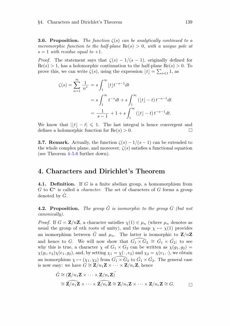
3.6. Proposition. The function ζ(s) can be analytically continued to ameromorphic function to the half-plane Re(s) > 0, with a unique pole ats = 1 with residue equal to +1.
Proof. The statement says that ζ(s) − 1/(s − 1), originally defined forRe(s) > 1, has a holomorphic continuation to the half-plane Re(s) > 0. Toprove this, we can write ζ(s), using the expression ⌊t⌋ =
∑n!t 1, as
ζ(s) =∞∑
n=1
1ns = s
∫ ∞
1⌊t⌋t−s−1dt
= s
∫ ∞
1t−sdt + s
∫ ∞
1(⌊t⌋ − t) t−s−1dt
= 1s − 1 + 1 + s
∫ ∞
1(⌊t⌋ − t) t−s−1dt.
We know that |⌊t⌋ − t| " 1. The last integral is hence convergent anddefines a holomorphic function for Re(s) > 0. #
3.7. Remark. Actually, the function ζ(s)− 1/(s− 1) can be extended tothe whole complex plane, and moreover, ζ(s) satisfies a functional equation(see Theorem 4-5.6 further down).
4. Characters and Dirichlet’s Theorem
4.1. Definition. If G is a finite abelian group, a homomorphism fromG to C∗ is called a character. The set of characters of G forms a groupdenoted by G.
4.2. Proposition. The group G is isomorphic to the group G (but notcanonically).
Proof. If G = Z/nZ, a character satisfies χ(1) ∈ µn (where µn denotes asusual the group of nth roots of unity), and the map χ '→ χ(1) providesan isomorphism between G and µn. The latter is isomorphic to Z/nZand hence to G. We will now show that !G1 × G2
∼= G1 × G2; to seewhy this is true, a character χ of G1 × G2 can be written as χ(g1, g2) =χ(g1, e2)χ(e1, g2), and, by setting χ1 = χ(· , e2) and χ2 = χ(e1, ·), we obtainan isomorphism χ '→ (χ1, χ2) from !G1 × G2 to G1 × G2. The general caseis now easy: we have G ∼= Z/n1Z × · · ·× Z/nrZ, hence
G ∼= (Z/n1Z × · · ·× Z/nrZ)b
∼= !Z/n1Z × · · ·× !Z/nrZ ∼= Z/n1Z × · · ·× Z/nrZ ∼= G. #

148 4. Analytic Number Theory
Dedekind zeta function of the field Q(exp(2πi/m)), which explains in amore conceptual manner why the coefficients are positive.
5. The Prime Number TheoremWe will prove the following form of the prime number theorem.
5.1. Theorem. The integral∫ ∞1 (θ(t) − t)t−2dt is convergent.
We will show that the convergence of this integral implies θ(x) ∼ x, andhence π(x) ∼ x/ log x. To see this, suppose that lim sup θ(x)x−1 > 1, thenthere exists ϵ > 0 and xn tending to infinity such that θ(xn)x−1
n ! 1 + ϵ.For t ∈ [xn, (1 + ϵ/2)xn], we therefore have
θ(t) − t
t2! θ(xn) − (1 + ϵ/2)xn
t2! ϵxn/2
t2! ϵxn
2(1 + ϵ/2)2x2n
,
and consequently∫ (1+ϵ/2)xn
xn
θ(t) − t
t2dt ! ϵ2
4(1 + ϵ/2)2,
which contradicts the convergence of the integral. We can therefore con-clude that lim sup θ(x)x−1 " 1. A symmetric argument shows thatlim inf θ(x)x−1 ! 1. It follows that lim θ(x)x−1 = 1.
To prove the theorem, we will use the following result from complex analysis(due to Newman, see [55, 81]) concerning the Laplace transform.
5.2. Theorem. (“The analytic theorem”) Let h(t) be a bounded, piecewisecontinuous function. Then the integral
F (s) =∫ +∞
0h(u)e−sudu
is convergent and defines a holomorphic function on the half-plane Re(s) >0. Suppose that this function can be analytically continued to a holomorphicfunction on the closed half-plane Re(s) ! 0. Then the integral convergesfor s = 0 and
F (0) =∫ +∞
0h(u)du.
Let us provisionally admit that this result is true and see how to apply it
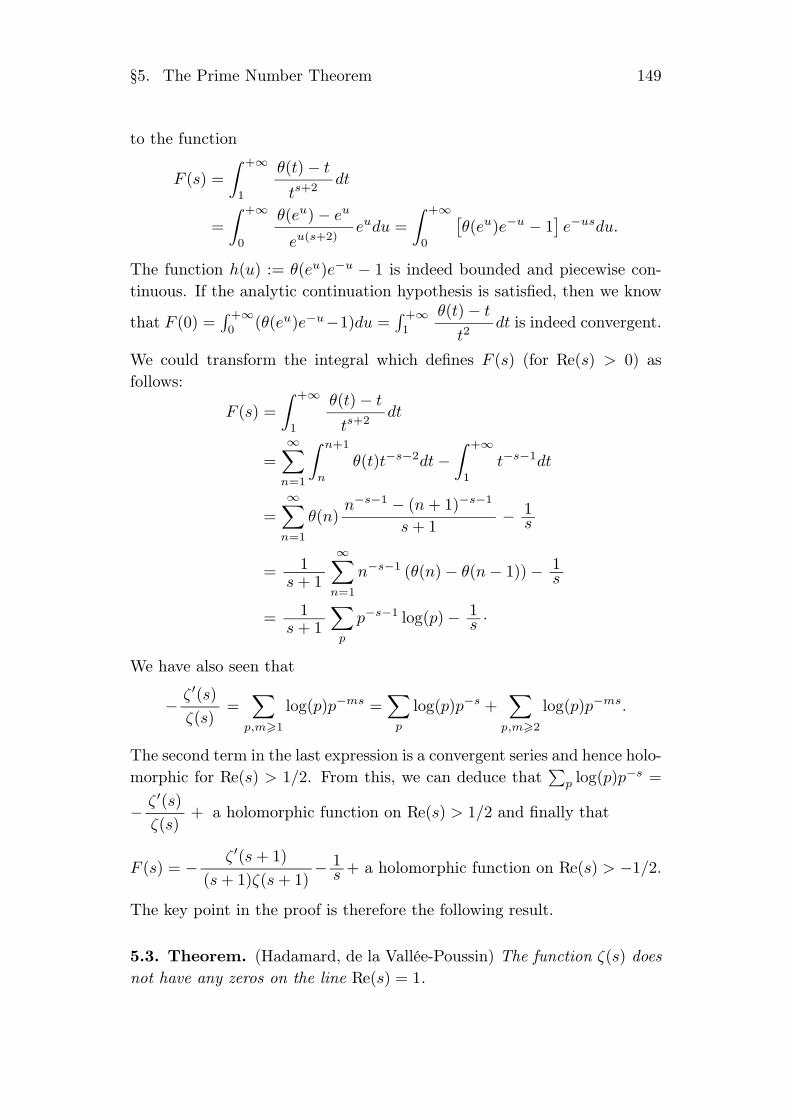
§5. The Prime Number Theorem 149
to the function
F (s) =∫ +∞
1
θ(t) − t
ts+2dt
=∫ +∞
0
θ(eu) − eu
eu(s+2)eudu =
∫ +∞
0
[θ(eu)e−u − 1
]e−usdu.
The function h(u) := θ(eu)e−u − 1 is indeed bounded and piecewise con-tinuous. If the analytic continuation hypothesis is satisfied, then we know
that F (0) =∫ +∞0 (θ(eu)e−u−1)du =
∫ +∞1
θ(t) − t
t2dt is indeed convergent.
We could transform the integral which defines F (s) (for Re(s) > 0) asfollows:
F (s) =∫ +∞
1
θ(t) − t
ts+2dt
=∞∑
n=1
∫ n+1
nθ(t)t−s−2dt −
∫ +∞
1t−s−1dt
=∞∑
n=1
θ(n)n−s−1 − (n + 1)−s−1
s + 1 − 1s
= 1s + 1
∞∑
n=1
n−s−1 (θ(n) − θ(n − 1)) − 1s
= 1s + 1
∑
p
p−s−1 log(p) − 1s ·
We have also seen that
−ζ ′(s)ζ(s)
=∑
p,m!1
log(p)p−ms =∑
p
log(p)p−s +∑
p,m!2
log(p)p−ms.
The second term in the last expression is a convergent series and hence holo-morphic for Re(s) > 1/2. From this, we can deduce that
∑p log(p)p−s =
−ζ ′(s)ζ(s)
+ a holomorphic function on Re(s) > 1/2 and finally that
F (s) = −ζ ′(s + 1)
(s + 1)ζ(s + 1)− 1
s + a holomorphic function on Re(s) > −1/2.
The key point in the proof is therefore the following result.
5.3. Theorem. (Hadamard, de la Vallée-Poussin) The function ζ(s) doesnot have any zeros on the line Re(s) = 1.
150 4. Analytic Number Theory
Proof. We start with the formula
4 cos(x) + cos(2x) + 3 = 2(1 + cos(x))2 ! 0.
Recall that
log ζ(σ + it) =∑
p,m
p−mσ−mit
m , and
log |ζ(σ + it)| =∑
p,m
p−mσ
m cos(mt log p).
This implies that
log(|ζ(σ + it)|4|ζ(σ + 2it)|ζ(σ)3
)
=∑
p,m!1
p−mσ
m (4 cos(mt log p) + cos(2mt log p) + 3) ! 0.
We can conclude from this, assuming σ > 1, that
|ζ(σ + it)|4|ζ(σ + 2it)|ζ(σ)3 ! 1. (4.22)
Now, if ζ(s) had a zero of order k at 1 + it and with order ℓ at 1 + 2it,then |ζ(σ + it)| ∼ a(σ − 1)k, |ζ(σ + 2it)| ∼ b(σ − 1)ℓ and ζ(σ) ∼ (σ − 1)−1
(where σ tends to 1 from above). The left-hand side of inequality (4.22) istherefore (asymptotically) equivalent to c(σ− 1)4k+ℓ−3, which implies that4k + ℓ − 3 " 0, and hence k = 0. #
5.4. Corollary. The function defined on Re(s) > 1 by
G(s) := −ζ ′(s)sζ(s)
− 1s − 1
extends to a holomorphic function on Re(s) ! 1.
Proof. The previous theorem shows that the function ζ ′(s)/ζ(s) is holo-morphic on the line Re(s) = 1, except for s = 1. Consequently, thefunction G(s) also is. To study G(s) in a neighborhood of s = 1, weuse the fact that ζ(s) has a simple pole at s = 1, and consequentlyζ ′(s)/ζ(s) = −1/(s − 1) + g(s), where g(s) is holomorphic in a neigh-borhood of 1. Thus G(s) is indeed holomorphic in a neighborhood of 1 andhence on the line Re(s) = 1. #
Appendix. Proof of the “analytic theorem”
Recall the statement of the analytic result used in the proof of the primenumber theorem.
§5. The Prime Number Theorem 151
5.5. Theorem. If h(t) is a bounded piecewise continuous function, thenthe integral (the Laplace transform of h)
F (s) =∫ +∞
0h(u)e−sudu
is convergent and defines a function which is holomorphic on the half-planeRe(s) > 0. Suppose that this function can be analytically continued to aholomorphic function on the closed half-plane Re(s) ! 0. Then the integralfor s = 0 converges and
F (0) =∫ +∞
0h(u)du.
Proof. The first part is analogous to the theorem of convergence for Dirich-let series (see Exercise 4-6.2). We will therefore prove the second state-ment. For a (large) real number T , let FT (s) :=
∫ T0 h(t)e−stdt; these
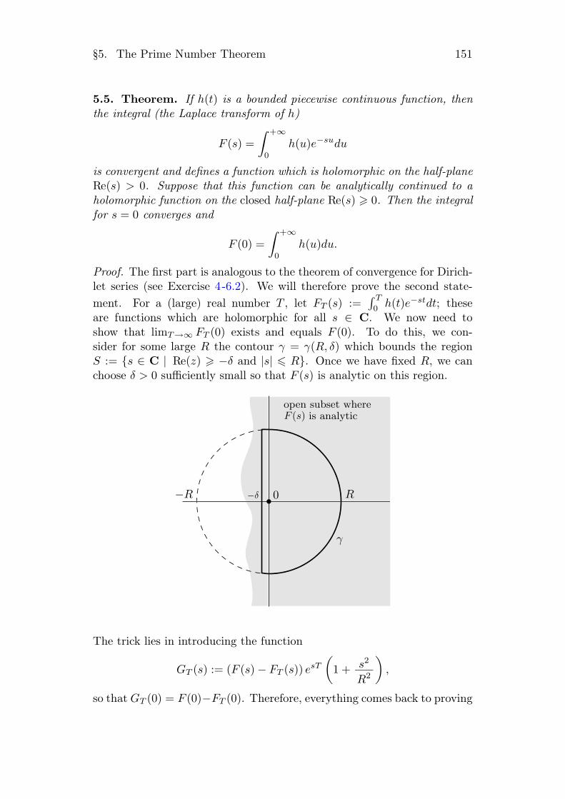
are functions which are holomorphic for all s ∈ C. We now need toshow that limT→∞ FT (0) exists and equals F (0). To do this, we con-sider for some large R the contour γ = γ(R, δ) which bounds the regionS := {s ∈ C | Re(z) ! −δ and |s| " R}. Once we have fixed R, we canchoose δ > 0 sufficiently small so that F (s) is analytic on this region.
The trick lies in introducing the function
GT (s) := (F (s) − FT (s)) esT
(1 + s2
R2
),
so that GT (0) = F (0)−FT (0). Therefore, everything comes back to proving
152 4. Analytic Number Theory
that limT→∞ GT (0) = 0. To do this, we will use the residue theorem a firsttime, noticing that
GT (0) = F (0) − FT (0) = 12πi
∫
γ(F (s) − FT (s)) esT
(1 + s2
R2
)dss ·
To find an upper bound on this integral, we cut the contour into two pieces:γ1, which is the piece of γ which lives in the half-plane Re(s) > 0, and γ2,which lives in the half-plane Re(s) < 0. We then carry out the followingcomputation.
Let s be a number such that |s| = R or s = Reiθ. Then we have∣∣∣∣e
sT
(1 + s2
R2
)1s
∣∣∣∣ = eRe(s)T∣∣e−iθ + eiθ
∣∣ 1R
= eRe(s)T 2 Re(s)R2
·
We also have the upper bound
|F (s) − FT (s)| =∣∣∣∣∫ ∞
Th(t)e−stdt
∣∣∣∣ " M
∫ ∞
T
∣∣e−st∣∣ dt = Me−Re(s)T
Re(s)·
This gives us∣∣∣∣
12πi
∫
γ1
(F (s) − FT (s)) esT
(1 + s2
R2
)dss
∣∣∣∣ " MR
·
Thus assuming that R is very large, this part of the integral will be ar-bitrarily small. Now, cut the integral over γ2 into two pieces, I1 and I2,where
I1 := 12πi
∫
γ2
F (s)esT
(1 + s2
R2
)dss ,
I2 := 12πi
∫
γ2
FT (s)esT
(1 + s2
R2
)dss ·
To find an upper bound on I2, observe first that FT (s) is entire. Theresidue theorem (or actually the Cauchy formula in this case) allows usto then replace the contour γ2 by the arc of a circle of radius R whichlives in the half-plane Re(s) < 0 and, by using the same upper bounds, toconclude that |I2| " M/R. To find an upper bound of I1, simply notice
that the function F (s)esT
(1 + s2
R2
)1s converges to 0 when T tends to
+∞ and converges uniformly on every compact set contained in Re(s) < 0.Consequently,
limT→∞
12πi
∫
γ2
F (s)esT
(1 + s2
R2
)dss = 0.
§5. The Prime Number Theorem 153
By putting the three upper bounds together, we see that
|FT (0) − F (0)| " 2MR
+ ϵ(T )
where ϵ(T ) tends to zero (in a way dependent on R). We needed to showthat limFT (0) = F (0), which is now accomplished. #
Supplement. Analytic continuation and the functional equationWe will now outline the main steps of the proof of the following theoremdue to Riemann.
5.6. Theorem. (The functional equation of the Riemann zeta function)The function ζ(s)−1/(s−1) can be analytically continued to the whole com-plex plane. Furthermore, the function ζ(s) satisfies the functional equationgiven by
ξ(s) = ξ(1 − s), (4.23)
where ξ(s) := π−s/2Γ(s/2)ζ(s).
As a preliminary, we will recall the construction of the function Γ(s) andthe Poisson formula which gives the functional equation for the theta series.
5.7. Lemma. The integral Γ(s) :=∫ ∞0 e−tts−1dt defines a holomorphic
function for Re(s) > 0, which satisfies the functional equation Γ(s + 1) =sΓ(s). It can be continued to all of C as a meromorphic function withsimple poles at 0,−1,−2,−3, . . . .
Proof. Showing that the integral is convergent does not pose any problems.The functional equation can be obtained by integrating by parts. Thefunctional equation also allows us to analytically continue by induction fromRe(s) > −n to Re(s) > −n − 1 by using the fact that Γ(s) = s−1Γ(s + 1).Finally, the expression
Γ(s) = 1s(s + 1) · · · (s + n)
Γ(s + n + 1)
makes it clear where the poles are. #
We can also prove that for all s, Γ(s) = 0 (see Exercise 4-6.19).
5.8. Lemma. (Poisson formula) Let f(x) be an integrable function overR (i.e., in L1(R)). We define its Fourier transform by
f(y) :=∫ +∞
−∞f(x) exp(2πixy)dx
154 4. Analytic Number Theory
and assume that the function∑
n∈Z f(x + n) is of bounded variation on[0, 1] and continuous. Then the following formula holds:
∑
n∈Z
f(n) =∑
m∈Z
f(m). (4.24)
Proof. We introduce the function G(x) :=∑
n∈Z f(x + n) (the hypothesesguarantee the existence and continuity of such a function), which is clearlya periodic function. Dirichlet’s theorem on Fourier series allows us to writeits Fourier expansion as
G(x) =∑
m∈Z
G(m) exp(2πimx),
where the Fourier coefficients can be calculated as follows:
G(m) :=∫ 1
0G(t) exp(−2πimt)dt =
∑
n∈Z
∫ 1
0f(t + n) exp(−2πimt)dt
=∫ +∞
−∞f(x) exp(−2πixm)dx = f(−m).
This gives ∑
n∈Z
f(x + n) =∑
m∈Z
f(m) exp(−2πimx).
The Poisson formula follows from that by taking x = 0. #
This formula is most often applied to a function f which is continuouslydifferentiable and fast decreasing (i.e., f(x) = O(|x|−M ) for all M), andtherefore the function G is itself continuously differentiable. This is thecase when applying the formula to the following “theta” function.
5.9. Corollary. The function2 θ(u) :=∑
n∈Z exp(−πun2
)satisfies the
functional equation for all u ∈ R∗+ given by:
θ(1/u) =√
u θ(u). (4.25)
Proof. It suffices to apply the Poisson formula to the function f(x) =exp(−πux2) and to verify that f(y) = exp(−πy2/u)/
√u. #
Proof. (of Theorem 4-5.6) We start with the following computation (where
2We hope that the context will allow the reader to distinguish this function from theTchebychev function θ(x) =
Pp"x log p.

§5. The Prime Number Theorem 155
we introduce t = πn2u) which is valid for Re(s) > 1.
ξ(s) = π−s/2Γ(s/2)ζ(s) =∑
n!1
∫ ∞
0e−tts/2π−s/2n−s dt
t
=∫ ∞
0
⎧⎨
⎩∑
n!1
exp(−πun2)
⎫⎬
⎭us/2 duu
=∫ ∞
0θ(u) us/2du
u
where
θ(u) :=∑
n!1
exp(−πun2
)=
θ(u) − 12 ·
Let us point out that θ(u) = O(exp(−πu)) when u tends to infinity andthat the functional equation of the function θ can be translated into
θ(
1u
)=
√u θ(u) + 1
2(√
u − 1). (4.26)
By using the simple computation∫ ∞1 t−s = 1/(s − 1) and the functional
equation of the theta function (4.25), we obtain
ξ(s) =∫ 1
0θ(u) us/2du
u +∫ ∞
1θ(u) us/2du
u
=∫ ∞
1θ(1/u) u−s/2du
u +∫ ∞
1θ(u) us/2du
u
=∫ ∞
1
{√uθ(u) + 1
2(√
u − 1)} u−s/2du
u +∫ ∞
1θ(u) us/2du
u
=∫ ∞
1θ(u)
{u
s2 + u
1−s
2
}duu + 1
s − 1 − 1s ·
We have a priori obtained the desired expression only for Re(s) > 1,but we can easily see that the integral defines an entire function sinceθ(u) = O(exp(−πu)) and since it is symmetric under the transformations '→ 1 − s. #
Supplement without proofs
1) To establish the prime number theorem, we could, in the place of the “an-alytic theorem”, use Ikehara’s theorem [40] (sometimes called the Ikehara-Wiener theorem), which is more powerful but also more tricky to prove. Wewill settle with stating the theorem. Its extension to the case of a multiplepole was proven by Delange [25].
40 P. COLMEZ
seulement si son terme general tend vers 0), nous avons consacre un chapitre aleur construction (la construction du corps Cp est un peu plus longue que cellede C, mais pas beaucoup) et un chapitre a l’analyse sur Zp. Le dernier chapitreest, quant a lui, consacre a la construction de la fonction zeta p-adique. Lesecond chapitre contient beaucoup plus de choses que ce qui est necessaire pourcette construction (les mesures suffiraient, mais les distributions deviennentindispensables pour construire des fonction L p-adiques plus generales, parexemple celles attachees aux formes modulaires). Pour d’autres points de vuesur les nombres p-adiques, le lecteur pourra consulter les livres p-adic numbers,
p-adic analysis, and zeta-functions et p-adic analysis : a short course on recent
work de Koblitz ou An introduction to G-functions de Dwork, Gerotto etSullivan. L’enonce precis du theoreme de Mazur et Wiles n’est pas donne dansle texte, pas plus que l’application au theoreme de Kummer et nous renvoyonsle lecteur interesse aux livres Introduction to cyclotomic fields de Washingtonou Cyclotomic fields I and II de Lang (pour le theoreme de Kummer, on peutaussi lire la demonstration dans l’ouvrage de Borevich et Chafarevitch dejacite).
CHAPITRE I
LA FONCTION ZETA DE RIEMANN
I.1. Prolongement analytique et valeurs aux entiers negatifs
Soit ζ(s) =!+∞
n=1 n−s ="
p(1 − p−s)−1 la fonction zeta de Riemann. Soit
Γ(s) =
# +∞
t=0e−tts
dt
tla fonction Γ d’Euler. Cette fonction est holomorphe
pour Re(s) > 0 et satisfait l’equation fonctionnelle Γ(s + 1) = sΓ(s), ce quipermet de la prolonger en une fonction meromorphe sur C tout entier.
Lemme I.1.1. Si Re(s) > 1, alors
ζ(s) =1
Γ(s)
# +∞
0
1
et − 1ts
dt
t.
Demonstration. Il suffit d’ecrire1
et − 1sous la forme
!+∞n=1 e−nt et d’utiliser
la formule
# +∞
0e−ntts
dt
t=
Γ(s)
ns.
ARITHMETIQUE DE LA FONCTION ZETA 41
Proposition I.1.2. Si f est une fonction C∞ sur R+ a decroissance rapide a
l’infini, alors la fonction
L(f, s) =1
Γ(s)
# +∞
0f(t)ts
dt
t
definie pour Re(s) > 0 admet un prolongement holomorphe a C tout entier et,
si n ∈ N, alors L(f,−n) = (−1)nf (n)(0).
Demonstration. Soit ϕ une fonction C∞ sur R+, valant 1 sur [0, 1] et 0 sur[2,+∞[. On peut ecrire f sous la forme ϕf+ (1 − ϕ)f et L(f, s) sous laforme L(ϕf, s) + L((1−ϕ)f, s) et comme (1−ϕ)f est nulle dans un voisinage
de 0 et a decroissance rapide a l’infini, l’integrale
# +∞
0f(t)ts
dt
tdefinit une
fonction holomorphe sur C tout entier. Comme de plus, 1/Γ(s) s’annule auxentiers negatifs, on a L((1− ϕ)f,−n) = 0 si n ∈ N. On voit donc que, quittea remplacer f par (1 − ϕ)f , on peut supposer f a support compact. Uneintegration par partie nous fournit alors la formule L(f, s) = −L(f ′, s + 1) siRe(s) > 1, ce qui permet de prolonger L(f, s) en une fonction holomorphe surC tout entier. D’autre part, on a
L(f,−n) = (−1)n+1L(f (n+1), 1) = (−1)n+1# +∞
0f (n+1)(t)dt = (−1)nf (n)(0),
ce qui termine la demonstration.
On peut en particulier appliquer cette proposition a f0(t) =t
et − 1. Soit
!+∞n=0 Bntn/n! le developpement de Taylor de f0 en 0. Les Bn sont des nombres
rationnels appeles nombres de Bernoulli et qu’on retrouve dans toutes lesbranches des mathematiques. On a en particulier
B0 = 1, B1 = −1
2, B2 =
1
6, B4 =
−1
30, . . . , B12 =
−691
2730,
et comme f0(t) − f0(−t) = −t, la fonction f0 est presque paire et B2k+1 = 0si k ! 1. Un test presque infaillible pour savoir si une suite de nombres a unrapport avec les nombres de Bernoulli est de regarder si 691 apparaıt dans lespremiers termes de cette suite.
Theoreme I.1.3(i) La fonction ζ a un prolongement meromorphe a C tout entier, holo-
morphe en dehors d’un pole simple en s = 1 de residu 1.
(ii) Si n ∈ Q, alors ζ(−n) = (−1)nBn+1
n + 1; en particulier, ζ(−n) ∈ Q.
Demonstration. On a ζ(s) = 1s−1L(f0, s−1) comme on le constate en utilisant
la formule Γ(s) = (s− 1)Γ(s − 1) ; on en deduit le resultat.
42 P. COLMEZ
I.2. Valeurs aux entiers positifs pairs
Proposition I.2.1. Si z ∈ C− Z, alors
1
z+
+∞$
n=1
% 1
z + n+
1
z − n
&= πcotg πz.
Demonstration. Notons F(z) la fonction
F(z) =1
z+
+∞$
n=1
% 1
z + n+
1
z − n
&=
1
z+
+∞$
n=1
2z
z2 − n2.
La convergence absolue de la serie dans le second membre montre que F(z)est une fonction meromorphe sur C, holomorphe sur C − Z avec des polessimples de residu 1 en les entiers, que F est impaire et periodique de periode 1.La fonction G(z) = F(z) − πcotg πz est donc holomorphe sur C, impaire etperiodique de periode 1.
Si −1/2 " x " 1/2, on a |z2 − n2| ! y2 + n2 − 1/4 et |z| " y + 1/2. Onobtient donc
'''+∞$
n=1
2z
z2 − n2
''' "
+∞$
n=1
'''2z
z2 − n2
''' "
+∞$
n=1
2y + 1
y2 − 14 + n2
"
# +∞
0
2y + 1
y2 − 14 + x2
dx =π
2·
2y + 1(
y2 − 14
.
Comme la fonction πcotg πz est bornee sur |Im(z)| ! 1, il existe c > 0 telque |G(z)| " c si z = x + iy et −1/2 " x " 1/2, y ! 1. De plus, G etantholomorphe, il existe c′ > 0 tel que |G(z)| " c′ si z = x + iy et −1/2 " x "
1/2, 0 " y " 1 et G etant impaire et periodique de periode 1, on a alors|G(z)| " sup(c, c′) quel que soit z ∈ C. La fonction G est donc bornee sur C
tout entier, donc constante et nulle car impaire. Ceci permet de conclure.
Maintenant, on a d’une part
1
z+
+∞$
n=1
2z
z2 − n2=
1
z−
+∞$
n=1
2z+∞$
k=0
z2k
n2k+2=
1
z− 2
+∞$
k=1
ζ(2k)z2k−1,
et d’autre part,
πcotg πz = iπe2iπz + 1
e2iπz − 1= iπ +
2iπ
e2iπz − 1= iπ +
1
z
+∞$
n=0
Bn(2iπz)n
n!.
On en deduit le resultat suivant.

ARITHMETIQUE DE LA FONCTION ZETA 43
Theoreme I.2.2. Si k est un entier ! 1, alors
ζ(2k) = −1
2B2k
(2iπ)2k
(2k)!.
En particulier, π−2kζ(2k) est un nombre rationnel.
I.3. Polylogarithmes et valeurs aux entiers positifs
de la fonction zeta
1. Polylogarithmes
Si k est un entier ! 1, on note Lik(z) la fonction definie, pour |z| < 1, parla formule
Lik(z) =+∞$
n=1
zn
nk.
Ces fonctions Lik, appelees polylogarithmes (Li2 est le dilogarithme, Li3 letrilogarithme. . .), ont ete introduites par Leibnitz, mais n’ont commence ajouer un role important que depuis une vingtaine d’annees ; on s’est apercurecemment qu’elles apparaissaient naturellement dans de multiples questions(volumes de varietes hyperboliques, valeurs aux entiers des fonctions zetas,cohomologie de GLn(C)...).
On a Li1(z) = − log(1 − z), etd
dzLik(z) = z−1Lik−1(z), ce qui permet
de prolonger analytiquement Lik(z), par recurrence sur k, en une fonctionholomorphe multivaluee sur C − {0, 1}. (On est oblige de supprimer 0 bienque la serie
!+∞n=1 zn/nk n’ait pas de singularite en 0 car, apres un tour autour
de 1, la fonction Li1(z) = − log(1− z) augmente de 2iπ et donc vaut 2iπ en 0,ce qui fait que Li2(z) =
)z−1Li1(z) a une singularite logarithmique en 0.)
Pour prolonger analytiquement log z et les Lik(z), k ! 1, il faut choisir unchemin γz dans C − {0, 1} reliant un point fixe (nous prendrons 1/2 commepoint de base de tous nos chemins) a z et poser
log z = − log 2 +
#
γz
dt
t,
Li1(z) = log 2 +
#
γz
dt
1− t
Lik(z) =+∞$
n=1
2−n
nk+
#
γz
Lik−1(t)dt
t.et
ARITHMETIQUE DE LA FONCTION ZETA 51
Cette formule etant valable quel que soit ϕ, la formule d’inversion de Fourier!!ϕ(0) = ϕ(0) nous permet de d’obtenir l’egalite
cn = ζ(n)cn−1
qui permet de conclure.
Remarque I.3.9. En voyant la formule du theoreme, on se dit qu’il doit existerune « decomposition » de SLn en morceaux refletant la factorisation naturelledu volume de SLn(R)/SLn(Z). C’est cette vague intuition qui mene a laK-theorie et aux regulateurs de Borel (cf. demonstration du theoreme I.3.7).
I.4. Equation fonctionnelle de la fonction zeta
Soit ξ(s) = π−s/2Γ(s/2)ζ(s).
Theoreme I.4.1. La fonction ξ(s) admet un prolongement meromorphe a C tout
entier, holomorphe en dehors de poles simples de residus respectifs −1 et 1 en
s = 0 et s = 1, et verifie l’equation fonctionnelle
ξ(s) = ξ(1− s).
Demonstration. Il y a un nombre assez consequent de methodes pour arri-ver au resultat. Nous en donnerons deux dans ce no et une autre au § III.4(cf. th. III.4.5).
1. Premiere methode : la fonction theta
Si t > 0, on a" +∞
−∞e−πtx2
e−2iπxydx = e−πt−1y2" +∞
−∞e−πt(x+it−1y)2dx = t−1/2e−πt−1y2
.
(C’est classique ; faire le changement de variables u =√
t(x + it−1y), uti-liser le theoreme des residus pour revenir sur la droite reelle et la formule# +∞−∞ e−πu2
du = 1 pour conclure.)
Si t > 0, soit θ(t) =$
n∈Z e−πtn2. La formule de Poisson
%
n∈Z
ϕ(n) =%
n∈Z
" +∞
−∞ϕ(x)e−2iπnxdx,
utilisee pour ϕ(x) = e−πtx2, nous fournit l’equation fonctionnelle
θ(t) = t−1/2θ(t−1).
52 P. COLMEZ
On a alors
ξ(s) =1
2
" +∞
0(θ(t)− 1)ts/2 dt
t
=1
2
" 1
0(t−1/2θ(t−1)− 1)ts/2 dt
t+
1
2
" +∞
1(θ(t)− 1)ts/2 dt
t
et on peut changer t en t−1 dans la premiere integrale pour obtenir
ξ(s) = −1
s+
1
s− 1+
1
2
" +∞
1(θ(t)− 1)(ts/2 + t(1−s)/2)
dt
t.
On en deduit le resultat car θ(t)− 1 est a decroissance rapide a l’infini, ce quiimplique que l’integrale est une fonction holomorphe de s sur C tout entier,et le membre de droite est evidemment invariant par s #→ 1− s.
2. Deuxieme methode : integrale sur un contour
Si c > 0, soit Cc le contour obtenu en suivant la droite reelle de +∞ a cπ,puis en parcourant le carre de sommets cπ(±1±i) dans le sens trigonometrique,et en retournant en +∞ le long de l’axe reel. Soit
Fc(s) =
"
Cc
1
ez − 1(−z)s
dz
z,
ou (−z)s = exp(s log(−z)) et la branche du logarithme choisie est celle dontla partie imaginaire est comprise entre −π et π ; en particulier, on a (−z)s =e−iπszs de +∞ a cπ et (−z)s = eiπszs de cπ a +∞ (apres avoir parcouru lecarre). Comme 1
ez−1 est a decroissance rapide a l’infini, la fonction Fc(s) estholomorphe sur C pour tout c qui n’est pas un entier pair (pour eviter les polesde 1
ez−1). D’autre part, le theoreme des residus montre que Fc(s) ne dependpas de c si c reste dans un intervalle du type ]2N, 2N + 2[, avec N ∈ N. Enparticulier, on a F1(s) = Fc(s) quel que soit c ∈ ]0, 2[. Si Re(s) > 1, quand ctend vers 0, l’integrale sur le carre de sommets cπ(±1 ± i) tend vers 0, et onobtient, en passant a la limite
F1(s) = e−iπs" 0
+∞
1
ez − 1zs dz
z+eiπs
" +∞
0
1
ez − 1zs dz
z= 2i · sin πs ·Γ(s) ·ζ(s).
Maintenant, quand N tend vers +∞, la fonction F2N+1(s) tend vers 0 quandRe(s) < 0 car 1
ez−1 est majoree, independamment de N, sur C2N+1. Ladifference entre F1(s) et F2N+1(s) peut se calculer grace au theoreme desresidus. La fonction 1
ez−1(−z)s−1 a des poles en z = ±2iπ,±4iπ, . . . ,±2Niπdans le contour delimite par la difference entre C2N+1 et C1. Si k ∈ {1, . . . ,N},le residu de 1
ez−1(−z)s−1 est (2kπ)s−1e−iπ(s−1)/2 en 2ikπ et (2kπ)s−1eiπ(s−1)/2
ARITHMETIQUE DE LA FONCTION ZETA 53
en −2ikπ, ce qui nous donne
1
2iπ(F2N+1(s)− F1(s)) = 2 cos π
s− 1
2·
N%
k=1
(2kπ)s−1.
En passant a la limite, on obtient donc F1(s) = 4iπ·cos(π s−12 )·(2π)s−1 ·ζ(1−s),
si Re(s) < 0. On en deduit l’equation fonctionnelle
sinπs · Γ(s) · ζ(s) = cos πs− 1
2· (2π)s · ζ(1− s).
Pour passer de cette equation fonctionnelle a celle de ξ, il faut utiliser lesformules classiques
Γ(s)Γ(1− s) =π
sinπs, Γ
&s2
'Γ&s + 1
2
'= 21−sΓ
&12
'Γ(s), et Γ
&12
'=√π.
I.5. Fonctions L de Dirichlet
1. Caracteres de Dirichlet et sommes de Gauss
Si d est un entier, on appelle caractere de Dirichlet modulo d un morphismede groupes de (Z/dZ)∗ dans C∗. L’image d’un caractere de Dirichlet est bienevidemment incluse dans le groupe des racines de l’unite.
Si d′ est un diviseur de d et χ est un caractere de Dirichlet modulo d′, onpeut aussi voir χ comme un caractere de Dirichlet modulo d en composant χavec la projection (Z/dZ)∗ → (Z/d′Z)∗. On dit que χ est de conducteur d sion ne peut pas trouver de diviseur d′ de d distinct de d, tel que χ provienned’un caractere modulo d′. De maniere equivalente, χ est de conducteur d siquel que soit d′ diviseur de d distinct de d, la restriction de χ au noyau de laprojection (Z/dZ)∗ → (Z/d′Z)∗ n’est pas triviale.
Si χ est un caractere de Dirichlet modulo d, on note χ−1 le caractere deDirichlet modulo d defini par χ−1(n) = (χ(n))−1 si n ∈ (Z/dZ)∗.
Si χ est un caractere de Dirichlet modulo d, on considere aussi souvent χcomme une fonction periodique sur Z de periode d en composant χ avec laprojection naturelle de Z sur Z/dZ et en etendant χ par 0 sur les entiers nonpremiers a d. On a donc χ−1(n) = (χ(n))−1 si (n, d) = 1, mais χ−1(n) = 0 si(n, d) = 1.
Si d est un entier, χ un caractere de Dirichlet de conducteur d et si n ∈ Z,on definit la somme de Gauss tordue G(χ, n) par la formule
G(χ, n) =%
a mod d
χ(a)e2iπna/d
et on pose G(χ) = G(χ, 1).