the relationship between technological development paths and the

ISSN 1341-4356 CGER-REPORT / CGER-I044-2000

The Relationship between Technological Development Paths and the Stabilization of Atmospheric Greenhouse Gas Concentrations

in Global Emissions Scenarios

Tsuneyuki Morita, Nebosja Nakicenovic and John Robinson

Contributors: Junich Fujino, Kejun Jiang, Shunsuke Mori, Hugh Pitcher,

Keywan Riahi, R. Alexander Roehrl, Kenji Yamaji

Center of Global Environmental Research (CGER) National Institute for Environmental Studies

2

The Relationship between Technological Development Paths and the Stabilization of Atmospheric Greenhouse Gas Concentrations

in Global Emissions Scenarios†

Tsuneyuki Morita1), Nebosja Nakicenovic2) and John Robinson3)

1) National Institute for Environmental Studies of Japan

16-2, Onogawa, Tsukuba, 305-0053 Japan phone: +81-298-50-2541, fax: +81-298-50-2572, email: [email protected]

2) International Institute for Applied Systems Analysis A-2361 Laxenburg, Austria

phone: +43-2236-807-411, fax: +43 2236 807 488, email: [email protected] 3) Sustainable Development Research Institute, University of British Columbia

B5 2202 Main Mall, Vancouver V6T 1Z4 Canada phone: +1-604-822-8198, fax: +1-604-822-9191, email: [email protected]

Contributors:

Junich Fujino (Japan), Kejun Jiang (China), Shunsuke Mori (Japan), Hugh Pitcher

(USA), Keywan Riahi (IIASA), R. Alexander Roehrl (IIASA), Kenji Yamaji (Japan)

Abstract This paper compares technological development paths that determine future mitigation

scenarios aimed at stabilizing atmospheric CO2 concentrations. Future social and economic

development paths have already been compared in relation to their impact on climate

mitigation by Morita, Nakicenovic and Robinson (2000). This paper is an expansion of that

earlier comparison. Forty stabilization scenarios are reviewed, and all use as their baseline the

new scenarios by the Intergovernmental Panel on Climate Change (IPCC) published in the

Special Report on Emission Scenarios (Nakicenovic et al, 2000).

Several common tendencies and characteristics can be observed across the scenarios. First, the

different technological development paths described in the baseline IPCC scenarios require

† As this study was supported by a database development program of CGER (Center of Global Environmental Research) which have been contributing to IPCC review processes, the opportunity to publish this paper was kindly given by CGER.

mailto:[email protected]



3

that: CO2 emissions be reduced by different levels; different schedules for the reductions be

adopted; and, different technology/policy measures be chosen to stabilize atmospheric CO2

concentrations - even to achieve the same stabilization level. Second, no one single measure is

sufficient for the development, adoption and diffusion of mitigation options to achieve

stabilization within the accepted time-frame. Third, the level of technology/policy measures

needed to achieve stabilization toward the end of the 21st century or beginning of the 22nd

century will be greatly affected by the choice of technological development paths over next

decades. The paper also identifies some characteristics in technological measures across the

different technological development paths to achieve the stabilization targets.

1. Introduction Future social and technological development paths will have a significant influence on global

climate change because these paths will determine levels of emissions of greenhouse gases

(GHG), such as CO2, and aerosols, such as SO2, and also strongly affect climate impacts,

adaptative capacity and mitigative capacity. Therefore, the policies and technologies to be

implemented to stabilize the future atmospheric GHG concentrations will depend on the paths

chosen for future development. This suggests that there is a wide range of policy/technology

options available to mitigate global climate by stabilizing GHG concentrations at a chosen

level.

To assess GHG stabilization technologies and policies, it is necessary to consider carefully the

range of possible assumptions about social and technological developments that underlie the

baseline scenarios of future economic development. The policy/technology options designed

to stabilize concentrations in a future world with reference to high baseline GHG emissions are

entirely different from those for a world with low baseline emissions. Also, it is necessary to

assess what packages of technology/policy measures are robust against different world

development paths.

The Intergovernmental Panel on Climate Change (IPCC) developed a set of new emission

scenarios based on a wide range of social and technological development paths. A range of

emission scenarios was quantified based on different future paths for economic social and

4

technological development, but they did not include any climate policy or mitigation measures

additional to those already in place. These scenarios are published in the “Special Report on

Emission Scenarios” by the IPCC (Nakicenovic et al., 2000) and are called SRES scenarios for

short.

The authors of this paper coordinated a special project to establish mitigation scenarios based

on these SRES scenarios. Nine modeling teams participated in the project and more than 70

mitigation scenarios were quantified based on the SRES scenarios. These are called

‘post-SRES’ scenarios.

A description and comparison of the post-SRES scenarios has already been published as a

special issue of the journal “Environmental Economics and Policy Studies”, and it focuses on

the differences in social development paths (Morita, Nakicenovic and Robinson, 2000). In that

paper, more than 40 stabilization scenarios, based on different social and economic

development paths, were compared and robust technology/policy measures were discussed in

relation to different future worlds and different stabilization targets. A key finding of this work

was that the future direction of technological development has significant implications for

future GHG emissions and aerosol emissions as well as future technological mitigation.

This paper extends the earlier work by providing an overview and comparison of the

post-SRES scenarios from the perspective of long-term technological development. First, the

technological development paths in the post-SRES are presented and compared to those in the

IPCC SRES baselines scenarios. Second, 41 post-SRES scenarios are compared. Third and

finally, several findings are summarized.

2. Quantification of new stabilization scenarios that use different technological

development paths.

The outline of SRES scenarios is summarized in Appendix 1. SRES scenarios comprise four

scenario families. One of the four families - the A1 family - contains very high economic

growth scenarios. It is characterized by a strong commitment to: education; high rates of

investment; various technology innovations; increased international mobility of people;

5

promotion and implementation of ideas; and, a general use of technology that has been

accelerated by advances in communication technologies.

With its high rate of economic growth, futures in the A1 family generate great pressures on the

energy resource base. As a result, this set of scenarios has a particularly large level of

uncertainty with regard to the future directions of technological progress in the energy field.

Thus, the A1 scenario family is divided into 3 groups that are each based on alternative

directions of technological change in the energy system.

The three A1 groups are distinguished by their technological emphasis: A1FI is a fossil fuel

intensive scenario, incorporating, for example, clean coal technologies and new technologies

for unconventional oil and gas; A1T has an emphasis on non-fossil fuel energy sources, such as

solar, wind, fuel cell, and nuclear technologies; and, A1B is balanced across all energy sources.

‘Balanced’ is defined as not relying too heavily on one particular energy source and

incorporates the assumption that similar improvement rates apply to all energy supplies and

end-use technologies.

The first stage of the post-SRES project to quantify mitigation scenarios based on SRES

focused on the differences in social and economic development paths among the four scenario

families. An outline of the first stage of the project is provided in Appendix 2.

In the second stage of the post-SRES project, additional comparisons among technological

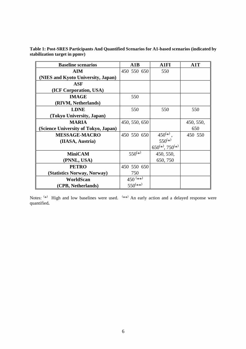
development were conducted. Table 1 shows the 41 scenarios that enable a comparison of

different development paths.

Five modeling teams - AIM, LDNE, MARIA, MESSAGE-MACRO and MiniCAM - prepared

additional mitigation scenarios based on A1FI and A1T technology development paths. These

paths are compared with A1B scenarios for different stabilization targets. The technical

methodologies used to quantify the stabilization scenarios are explained in Appendix 2.

6

Table 1: Post-SRES Participants And Quantified Scenarios for A1-based scenarios (indicated by stabilization target in ppmv)

Notes: (*) High and low baselines were used. (**) An early action and a delayed response were quantified.

Baseline scenarios A1B A1FI A1T AIM

(NIES and Kyoto University, Japan) 450 550 650 550

ASF (ICF Corporation, USA)

IMAGE (RIVM, Netherlands)

550

LDNE (Tokyo University, Japan)

550 550 550

MARIA (Science University of Tokyo, Japan)

450, 550, 650 450, 550, 650

MESSAGE-MACRO (IIASA, Austria)

450 550 650 450(*) , 550(*)

650(*), 750(*)

450 550

MiniCAM (PNNL, USA)

550(*) 450, 550, 650, 750

PETRO (Statistics Norway, Norway)

450 550 650 750

WorldScan (CPB, Netherlands)

450 (**) 550(**)

7

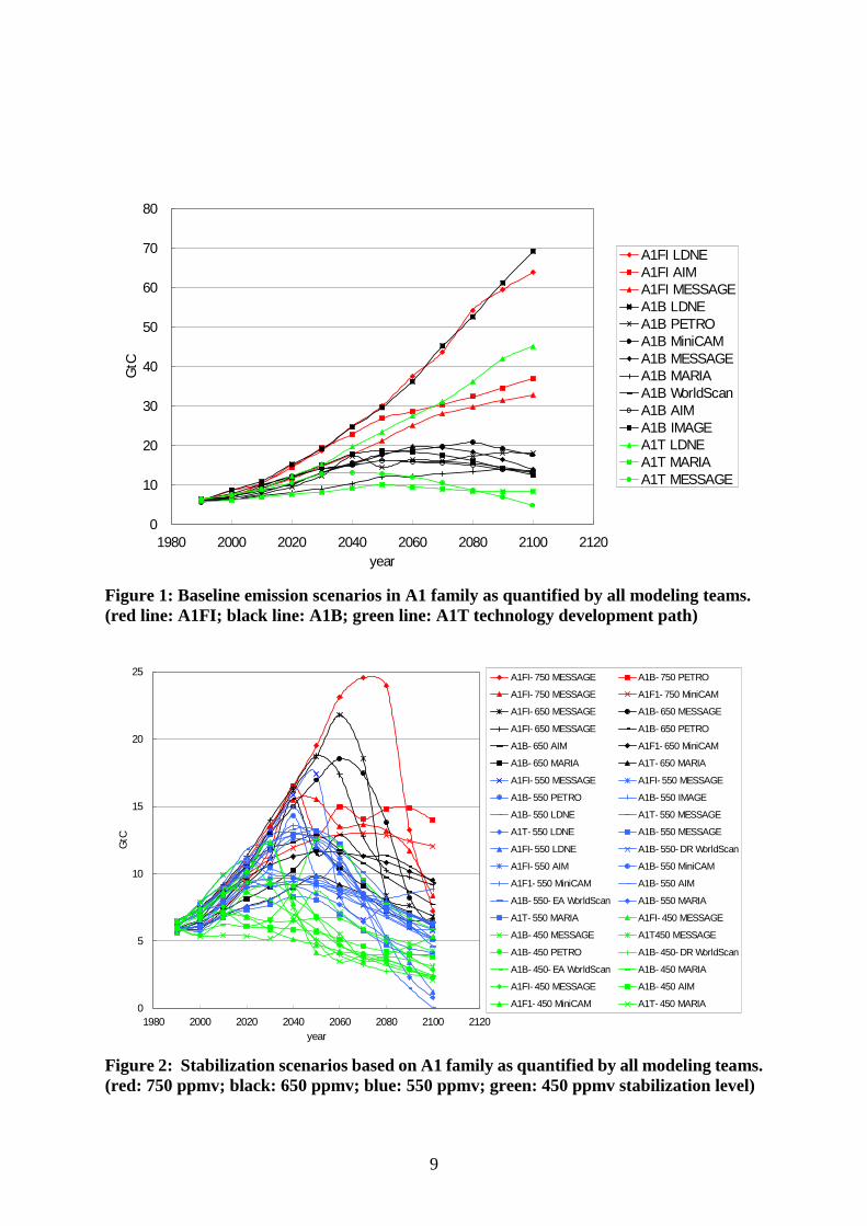
3. Comparison of stabilization scenarios Figure 1 shows CO2 emission scenarios used as the baselines for stabilization scenarios.

LDNE shows exceptionally high emissions, but it carries a great deal of uncertainty because of

a lack of time to harmonize all quantitative scenarios. As a result, the technological

development path of A1FI is considered to show the highest emission path and A1T is

considered to show the lowest emission path. The main conclusion from this comparison is

that technology developments determine to a large extent future CO2 emission trajectories.

These differences between the baseline scenarios imply differences in the amount by which the

concentration of atmospheric CO2 must be reduced to achieve stabilization. In turn, this

results in a selection of different technology/policy measures, and as a consequence it means

different financial costs to stabilize the CO2 concentration even at the same level in different

scenarios. Technological change is a key component in bringing down the cost of mitigation

options and their contribution to emission reductions.

Figure 2 shows stabilization scenarios based on different A1 development paths. It is clear that

stabilization targets at low levels require low emission trajectories and high stabilization levels

require high emission trajectories. This range of trajectories is caused by several factors, in

particular model structures that determine trajectory patterns, baseline emissions that

determine technology and policy options, and a carbon cycle model that determines the

cumulative emissions.

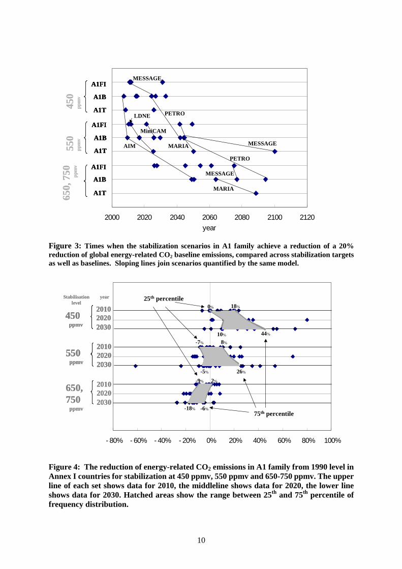
Figure 2 shows emissions paths of stabilization scenarios and thus does not directly indicate the

differences in technology development paths among stabilization scenarios. Figure 3

compares the times when the stabilization scenarios achieve a 20% reduction in relation to the

global baseline emissions. This figure compares not only technology development baselines

but also stabilization targets and illustrates in this way the difference among the technological

development paths across stabilization scenarios. As shown, the higher the level of baseline

emissions caused by the selected technology development path, as well as the lower the

stabilization level that is required, the earlier the emission reduction from the baseline level. It

must be stressed that technology/policy measures need to be introduced earlier if a fossil fuel

intensive technological development path is chosen.

8

Figure 4 was prepared to respond to a key policy question related to ‘reduction levels’ in the

first quarter of the 21st century. The ‘reduction level’ is the amount by which Annex 1

countries have to reduce their CO2 emissions from the 1990 level for the atmospheric CO2

concentration to be stabilized at 450 ppmv, 550 ppmv and 650-750 ppmv. In order to identify

a range of middle course scenarios, the figure shows the range between the 25th and 75th

percentile of frequency distribution. If an A1 world is selected over the next 100 years, the

Kyoto target becomes the minimum required to stabilize concentrations at 450 ppmv and 550

ppmv. If 450 ppmv is required, Annex 1 emission levels after 2010 have to be reduced much

more than the 2010 level. In the 550 ppmv stabilization scenario, the Kyoto commitment may

be adequate to achieve stabilization.

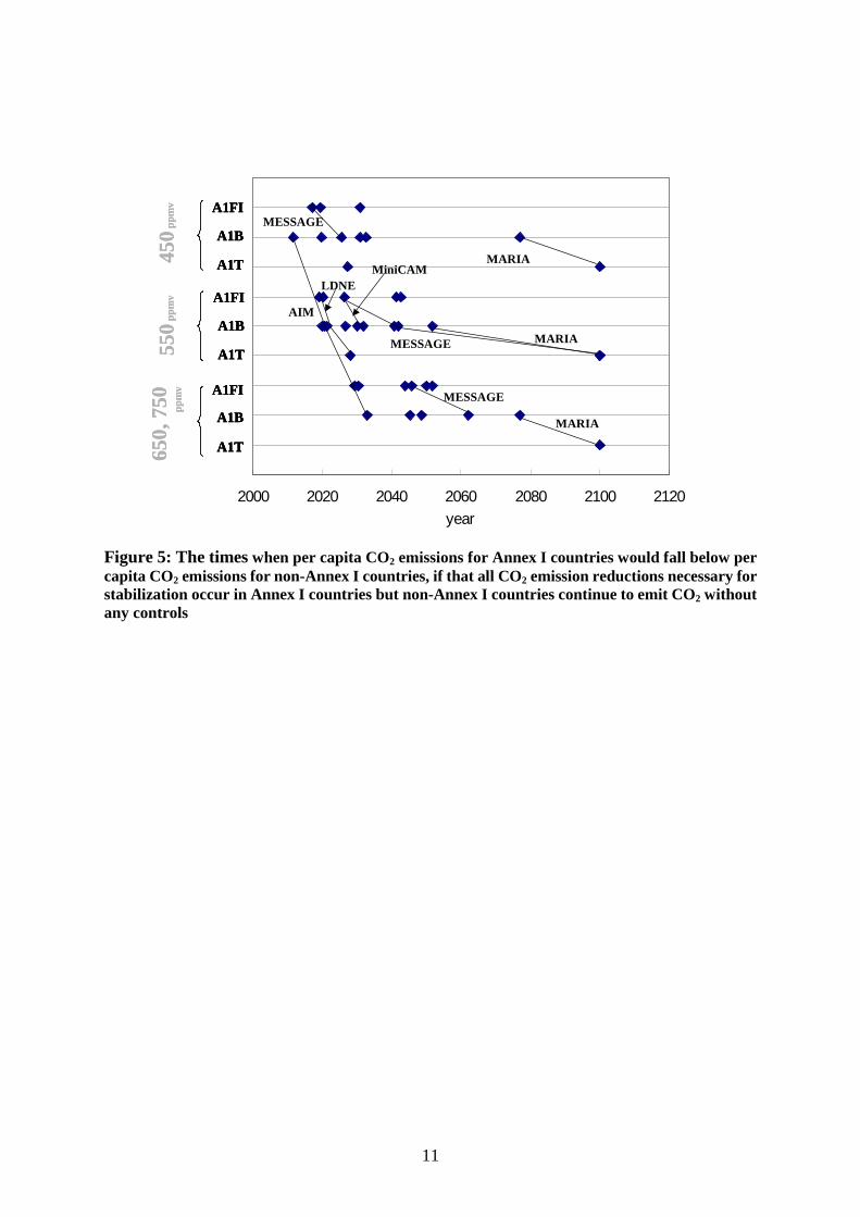
Figure 5 illustrates mitigation options for developing countries. It shows the times when per

capita CO2 emissions in Annex 1 countries fall below per capita CO2 emissions in non-Annex

1 countries based on the assumption that all CO2 emission reductions necessary to achieve

stabilization occur in Annex 1 countries while non-Annex 1 countries emit CO2 without any

controls. Most of the post-SRES scenarios based on A1 world indicate that per capita Annex I

emissions would fall below per capita non-Annex I emissions in the 21st century. This situation

occurs before 2050 in quarter of the scenarios. The times at which stabilization is achieved is

significantly affected by future technology development paths as well as stabilization targets.

As a result, the selection of technology development paths will strongly influence the time at

which developing countries will need to begin to diverge from baseline emissions.

9

Figure 1: Baseline emission scenarios in A1 family as quantified by all modeling teams. (red line: A1FI; black line: A1B; green line: A1T technology development path)

Figure 2: Stabilization scenarios based on A1 family as quantified by all modeling teams. (red: 750 ppmv; black: 650 ppmv; blue: 550 ppmv; green: 450 ppmv stabilization level)

0

10

20

30

40

50

60

70

80

1980 2000 2020 2040 2060 2080 2100 2120

year

GtC

A1FI LDNEA1FI AIMA1FI MESSAGEA1B LDNEA1B PETROA1B MiniCAMA1B MESSAGEA1B MARIAA1B WorldScanA1B AIMA1B IMAGEA1T LDNEA1T MARIAA1T MESSAGE

0

5

10

15

20

25

1980 2000 2020 2040 2060 2080 2100 2120

year

GtC

A1FI-750 MESSAGE A1B-750 PETRO

A1FI-750 MESSAGE A1F1-750 MiniCAM

A1FI-650 MESSAGE A1B-650 MESSAGE

A1FI-650 MESSAGE A1B-650 PETRO

A1B-650 AIM A1F1-650 MiniCAM

A1B-650 MARIA A1T-650 MARIA

A1FI-550 MESSAGE A1FI-550 MESSAGE

A1B-550 PETRO A1B-550 IMAGE

A1B-550 LDNE A1T-550 MESSAGE

A1T-550 LDNE A1B-550 MESSAGE

A1FI-550 LDNE A1B-550-DR WorldScan

A1FI-550 AIM A1B-550 MiniCAM

A1F1-550 MiniCAM A1B-550 AIM

A1B-550-EA WorldScan A1B-550 MARIA

A1T-550 MARIA A1FI-450 MESSAGE

A1B-450 MESSAGE A1T450 MESSAGE

A1B-450 PETRO A1B-450-DR WorldScan

A1B-450-EA WorldScan A1B-450 MARIA

A1FI-450 MESSAGE A1B-450 AIM

A1F1-450 MiniCAM A1T-450 MARIA

10

Figure 3: Times when the stabilization scenarios in A1 family achieve a reduction of a 20% reduction of global energy-related CO2 baseline emissions, compared across stabilization targets as well as baselines. Sloping lines join scenarios quantified by the same model.

Figure 4: The reduction of energy-related CO2 emissions in A1 family from 1990 level in Annex I countries for stabilization at 450 ppmv, 550 ppmv and 650-750 ppmv. The upper line of each set shows data for 2010, the middleline shows data for 2020, the lower line shows data for 2030. Hatched areas show the range between 25th and 75th percentile of frequency distribution.

2000 2020 2040 2060 2080 2100 2120

year

A1FI

A1B

A1T

A1FI

A1B

A1T

A1FI

A1B

A1T

450

ppm

v55

0pp

mv

650,

750 pp

mv

AIM

LDNE

MARIA

MARIA

MESSAGE

MESSAGE

MESSAGE

MiniCAM

PETRO

PETRO

2000 2020 2040 2060 2080 2100 2120

year

A1FI

A1B

A1T

A1FI

A1B

A1T

A1FI

A1B

A1T

450

ppm

v55

0pp

mv

650,

750 pp

mv

2000 2020 2040 2060 2080 2100 2120

year

A1FI

A1B

A1T

A1FI

A1B

A1T

A1FI

A1B

A1T

450

ppm

v55

0pp

mv

650,

750 pp

mv

A1FI

A1B

A1T

A1FI

A1B

A1T

A1FI

A1B

A1T

A1FI

A1B

A1T

A1FI

A1B

A1T

A1FI

A1B

A1T

450

ppm

v55

0pp

mv

650,

750 pp

mv

AIM

LDNE

MARIA

MARIA

MESSAGE

MESSAGE

MESSAGE

MiniCAM

PETRO

PETRO

-80% -60% -40% -20% 0% 20% 40% 60% 80% 100%

550ppmv

201020202030

yearStabilisation level

450ppmv

201020202030

650, 750

ppmv

201020202030

25th percentile

75th percentile

0% 18%

8%-7%

10% 44%

26%-5%

-9% 2%

-6%-18%

-80% -60% -40% -20% 0% 20% 40% 60% 80% 100%

550ppmv

201020202030


450ppmv

201020202030

650, 750

ppmv

201020202030

25th percentile

75th percentile

0% 18%

8%-7%

10% 44%

26%-5%

-9% 2%

-6%-18%

-80% -60% -40% -20% 0% 20% 40% 60% 80% 100%

550ppmv

201020202030


450ppmv

201020202030

650, 750

ppmv

201020202030

550ppmv

201020202030

550ppmv

201020202030


450ppmv

201020202030

450ppmv

201020202030

650, 750

ppmv

201020202030

25th percentile

75th percentile

0% 18%

8%-7%

10% 44%

26%-5%

-9% 2%

-6%-18%

11

Figure 5: The times when per capita CO2 emissions for Annex I countries would fall below per capita CO2 emissions for non-Annex I countries, if that all CO2 emission reductions necessary for stabilization occur in Annex I countries but non-Annex I countries continue to emit CO2 without any controls

2000 2020 2040 2060 2080 2100 2120

year

A1FI

A1B

A1T

A1FI

A1B

A1T

A1FI

A1B

A1T

450p

pmv

550p

pmv

650,

750 pp

mv

AIM

LDNE

MARIA

MARIA

MARIA

MESSAGE

MESSAGE

MESSAGE

MiniCAM

2000 2020 2040 2060 2080 2100 2120

year

A1FI

A1B

A1T

A1FI

A1B

A1T

A1FI

A1B

A1T

450p

pmv

550p

pmv

650,

750 pp

mv

2000 2020 2040 2060 2080 2100 2120

year

A1FI

A1B

A1T

A1FI

A1B

A1T

A1FI

A1B

A1T

450p

pmv

550p

pmv

650,

750 pp

mv

A1FI

A1B

A1T

A1FI

A1B

A1T

A1FI

A1B

A1T

A1FI

A1B

A1T

A1FI

A1B

A1T

A1FI

A1B

A1T

450p

pmv

550p

pmv

650,

750 pp

mv

AIM

LDNE

MARIA

MARIA

MARIA

MESSAGE

MESSAGE

MESSAGE

MiniCAM

12

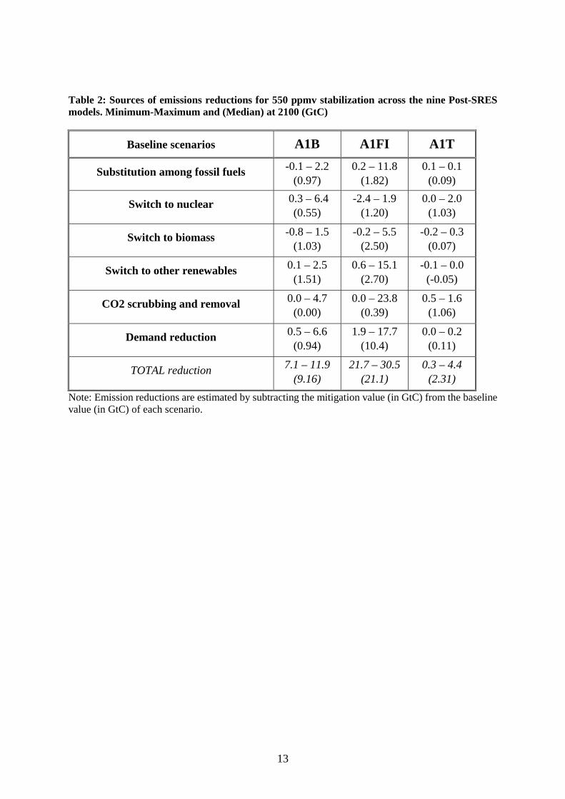
4. Comparison of technology/policy measures and assessment of robustness As discussed in the previous sections, the technology/policy measures required to achieve

stabilization are significantly affected by future technological development paths. To compare

the differences in technology/policy measures, the sources of emission reductions are

estimated in Table 2. This summarizes the contribution of several mitigation options and/or

measures for the post-SRES scenarios. The numbers represent the emission reduction (in Giga

tons of Carbon, GtC) between the baseline and the stabilization cases. For simplicity, the table

only shows the range from the maximum to the minimum as well as the medium value in 2100

for the 550 ppmv stabilization case. In the table, the demand reduction includes technological

efficiency improvements for both energy use technology and energy supply technology, social

efficiency improvements such as public transport introduction, dematerialization promoted by

lifestyle changes and the introduction of recycling systems

The following conclusions can be drawn from this table:

1) No single measure will be sufficient to stabilize atmospheric CO2 concentrations,

even if a specific technology development path is selected;

2) If a fossil fuel intensive technological development path is selected, the reduction in

end-use energy demand should become a very important countermeasure otherwise CO2

scrubbing and removal technology needs to be deployed. Substitution of fossil fuels is more

effective in conjunction with carbon removal and storage; and,

3) The contribution of energy demand reduction, substitution among fossil fuels and

switching to renewable energy are all relatively large. The contribution of nuclear energy and

CO2 scrubbing and removal differ significantly among the models and also across technology

development paths.

13

Table 2: Sources of emissions reductions for 550 ppmv stabilization across the nine Post-SRES models. Minimum-Maximum and (Median) at 2100 (GtC)

Baseline scenarios A1B A1FI A1T

Substitution among fossil fuels -0.1 – 2.2 (0.97)

0.2 – 11.8 (1.82)

0.1 – 0.1 (0.09)

Switch to nuclear 0.3 – 6.4 (0.55)

-2.4 – 1.9 (1.20)

0.0 – 2.0 (1.03)

Switch to biomass -0.8 – 1.5 (1.03)

-0.2 – 5.5 (2.50)

-0.2 – 0.3 (0.07)

Switch to other renewables 0.1 – 2.5 (1.51)

0.6 – 15.1 (2.70)

-0.1 – 0.0 (-0.05)

CO2 scrubbing and removal 0.0 – 4.7 (0.00)

0.0 – 23.8 (0.39)

0.5 – 1.6 (1.06)

Demand reduction 0.5 – 6.6 (0.94)

1.9 – 17.7 (10.4)

0.0 – 0.2 (0.11)

TOTAL reduction 7.1 – 11.9 (9.16)

21.7 – 30.5 (21.1)

0.3 – 4.4 (2.31)

Note: Emission reductions are estimated by subtracting the mitigation value (in GtC) from the baseline value (in GtC) of each scenario.

14

5. Concluding remarks Several main conclusions emerge from this review.

First, because the technological development paths are different, the CO2 emissions produced

by following each path must be reduced by different amounts. Each path requires the adoption

of different technology/policy measures and different financial expenditures to stabilize the

concentration of CO2 - even where the same concentration is achieved in different scenarios.

Second, the higher the level of baseline emissions and the lower the required stabilization level,

the earlier must the emission reduction from the baseline level must be achieved. It must be

stressed that technology/policy measures need to be introduced earlier in the first half of the

21st century if a fossil fuel intensive technological development path is chosen.

Third, the selection of technology development paths also determines the time at which

developing countries need to begin to diverge from the baseline emissions. Most of the

Post-SRES scenarios based on A1 world suggest that developing countries need to prepare to

diverge from baseline emissions in the first half of the 21st century.

Fourth, no single measure is sufficient to stabilize atmospheric CO2 concentrations,

independent of which specific baseline technology development path is selected. Therefore,

policy integration across an array of technologies, sectors and regions is essential if climate

policies are to be successful.

Fifth, energy demand reduction, substitution among fossil fuels and switching to renewable

energy sources make a relatively large contribution to the success of climate mitigation policies

across all different technological paths.

Finally, if a fossil fuel intensive technological development path is selected, the reduction in

end-use energy demand should become a very important countermeasure, otherwise CO2

scrubbing and removal technologies need to be developed.

15

This paper represents the early stages of systematic studies on the relationships between

technological development paths and climatic policy/technology measures. The potential for

more valuable work on this globally important topic is large. Analysis is needed of more

consistent relationships between technological development paths and technology options for

climatic stabilization. Mitigation scenarios in developing countries should be examined in

relation to the choice of future technological development paths. Also, studies are needed of

the effects of technological development paths on mitigation technologies to reduce

non-energy and non-CO2 gaseous emissions.

Most importantly, the feasibility and/or applicability of various technology options as well as

technological development path have to be examined more systematically in relation to the

socio-political assumptions underlying the different SRES baseline worlds. For example, the

choice of future development paths will influence or even determine some aspects of future

social structures. In turn, social structures will influence or determine whether a particular

technological development path is followed and/or a technology option accepted. In this

respect, a key area for future research lies in examining the degree of choice that exists with

respect to achieving different development paths, and the types of decisions and policies that

can be expected to reinforce or contribute to the achievement of such paths. It is more difficult

to provide clear answers to such qualitative issues. However as the analysis presented in this

paper suggests, the SRES and post-SRES approach of combining narrative storylines and

model quantifications opens the door to new approaches to considering of these critical

questions.

16

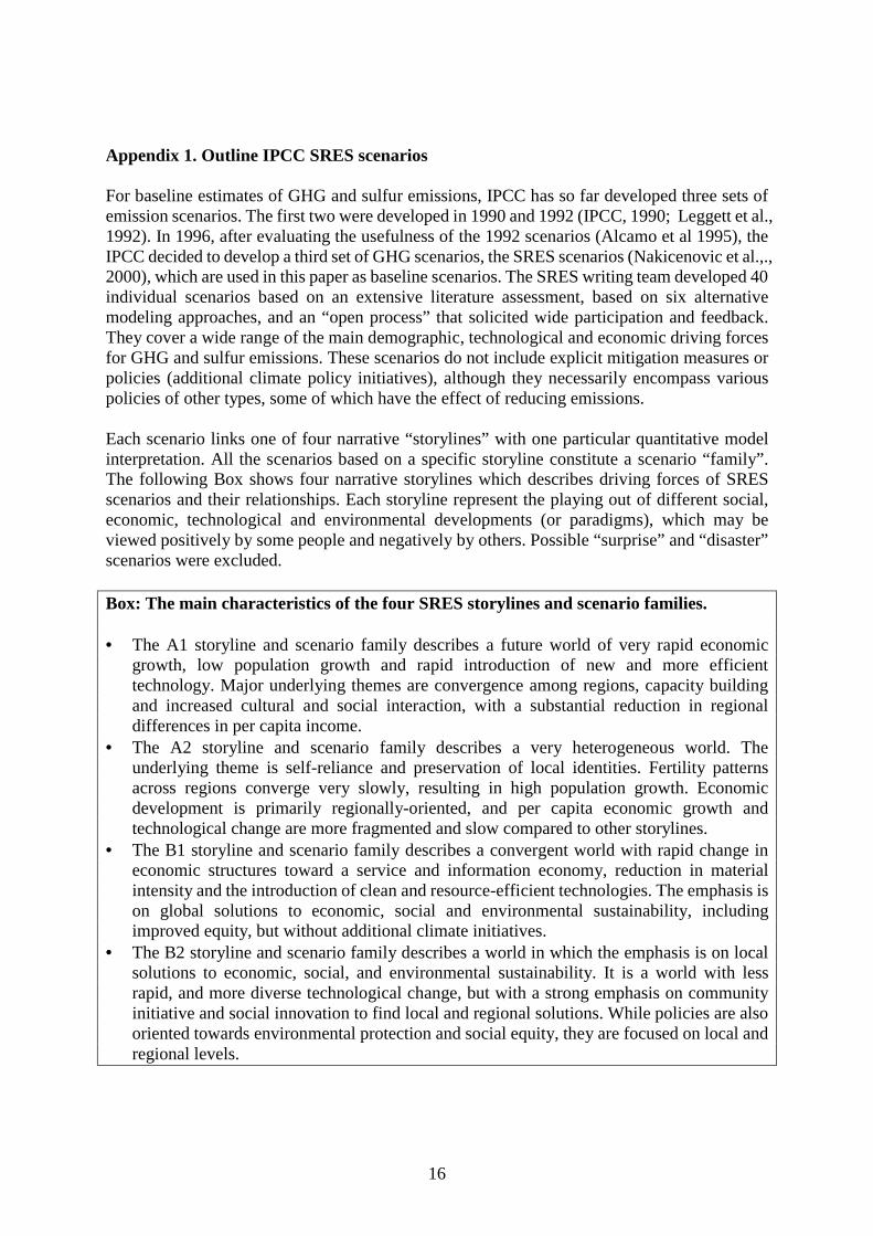
Appendix 1. Outline IPCC SRES scenarios For baseline estimates of GHG and sulfur emissions, IPCC has so far developed three sets of emission scenarios. The first two were developed in 1990 and 1992 (IPCC, 1990; Leggett et al., 1992). In 1996, after evaluating the usefulness of the 1992 scenarios (Alcamo et al 1995), the IPCC decided to develop a third set of GHG scenarios, the SRES scenarios (Nakicenovic et al.,., 2000), which are used in this paper as baseline scenarios. The SRES writing team developed 40 individual scenarios based on an extensive literature assessment, based on six alternative modeling approaches, and an “open process” that solicited wide participation and feedback. They cover a wide range of the main demographic, technological and economic driving forces for GHG and sulfur emissions. These scenarios do not include explicit mitigation measures or policies (additional climate policy initiatives), although they necessarily encompass various policies of other types, some of which have the effect of reducing emissions. Each scenario links one of four narrative “storylines” with one particular quantitative model interpretation. All the scenarios based on a specific storyline constitute a scenario “family”. The following Box shows four narrative storylines which describes driving forces of SRES scenarios and their relationships. Each storyline represent the playing out of different social, economic, technological and environmental developments (or paradigms), which may be viewed positively by some people and negatively by others. Possible “surprise” and “disaster” scenarios were excluded. Box: The main characteristics of the four SRES storylines and scenario families. • The A1 storyline and scenario family describes a future world of very rapid economic

growth, low population growth and rapid introduction of new and more efficient technology. Major underlying themes are convergence among regions, capacity building and increased cultural and social interaction, with a substantial reduction in regional differences in per capita income.

• The A2 storyline and scenario family describes a very heterogeneous world. The underlying theme is self-reliance and preservation of local identities. Fertility patterns across regions converge very slowly, resulting in high population growth. Economic development is primarily regionally-oriented, and per capita economic growth and technological change are more fragmented and slow compared to other storylines.

• The B1 storyline and scenario family describes a convergent world with rapid change in economic structures toward a service and information economy, reduction in material intensity and the introduction of clean and resource-efficient technologies. The emphasis is on global solutions to economic, social and environmental sustainability, including improved equity, but without additional climate initiatives.

• The B2 storyline and scenario family describes a world in which the emphasis is on local solutions to economic, social, and environmental sustainability. It is a world with less rapid, and more diverse technological change, but with a strong emphasis on community initiative and social innovation to find local and regional solutions. While policies are also oriented towards environmental protection and social equity, they are focused on local and regional levels.

17

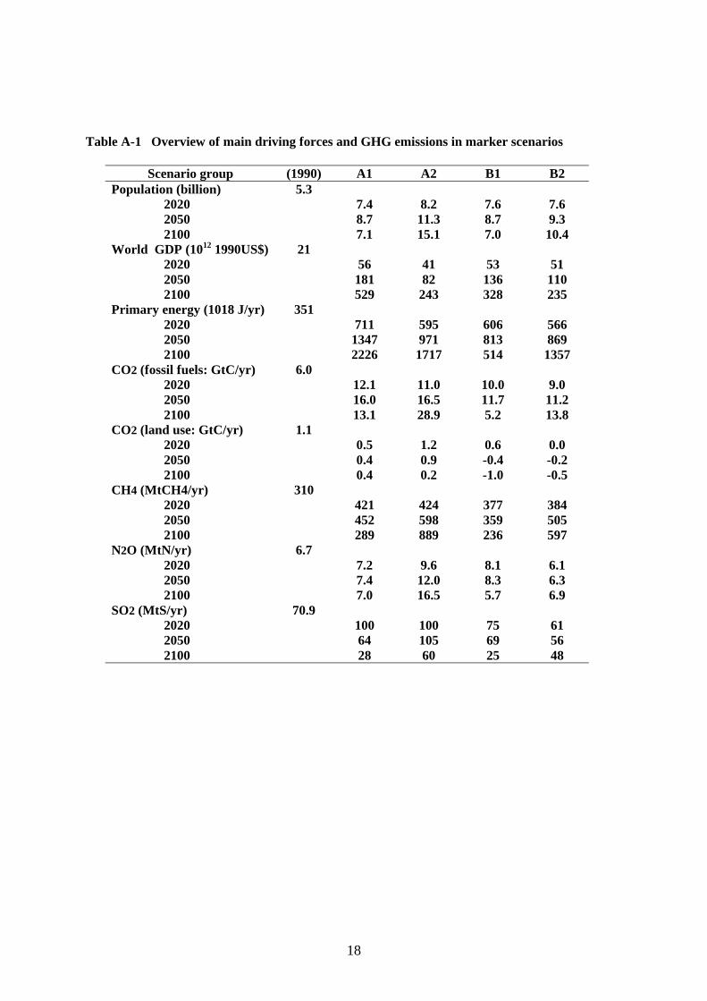
In addition, scenarios in the A1 family were categorized into three groups according to their technological emphasis -- on coal, oil and gas (A1FI), non-fossil energy sources (A1T) or a balance of all three (A1B). The last group, a balanced A1 is simply noted here as “A1”. Six different models, AIM, ASF, IMAGE, MARIA, MESSAGE-MACRO and MiniCAM were used that are representative of different modeling approaches and different integrated assessment frameworks in the literature. One preliminary scenario from each family, referred to as a “marker,” was posted on the SRES web site, and the markers were intensively tested for reproducibility using different modeling approaches with “harmonized” common assumptions of population growth, GDP growth, and final energy use. Table 1 summarizes the main demographic, technological, social and economic driving forces across the maker scenarios in 2050 and 2100. These drive the energy and land-use changes that are the major sources of GHG emissions. The 40 SRES scenarios cover most of the range of carbon dioxide, other GHG, and sulfur emissions found in the recent scenario literature. Table 1 summarizes main driving forces and GHG and sulfur emissions of the maker scenarios at 1990, 2020, 2050, and 2100 year. CO2 emissions in A1 are highest in growth rate in the first quarter of the 21st century, peak at the middle of the century in terms of absolute emission levels, and then decrease toward 2100. In A2, CO2 emissions are in the middle of the range of scenarios in the first half of 21 century, but become very high in the latter half of the century. In the B1 world, CO2 emissions decline after the second quarter of the 21st century even without any climate policy, and this scenario family has the lowest emission levels in the latter half of the century. CO2 emissions in B2 world are lowest in the first half of the 21st century, but continue to increase in the second half, and the emissions reach a similar level to that in A1 in 2100.

18

Table A-1 Overview of main driving forces and GHG emissions in marker scenarios

Scenario group (1990) A1 A2 B1 B2

Population (billion) 2020 2050 2100 World GDP (1012 1990US$) 2020 2050 2100 Primary energy (1018 J/yr) 2020 2050 2100 CO2 (fossil fuels: GtC/yr) 2020 2050 2100 CO2 (land use: GtC/yr) 2020 2050 2100 CH4 (MtCH4/yr) 2020 2050 2100 N2O (MtN/yr) 2020 2050 2100 SO2 (MtS/yr) 2020 2050 2100

5.3

21

351

6.0

1.1

310

6.7

70.9

7.4 8.7 7.1

56

181 529

711

1347 2226

12.1 16.0 13.1

0.5 0.4 0.4

421 452 289

7.2 7.4 7.0

100 64 28

8.2

11.3 15.1

41 82

243

595 971

1717

11.0 16.5 28.9

1.2 0.9 0.2

424 598 889

9.6

12.0 16.5

100 105 60

7.6 8.7 7.0

53

136 328

606 813 514

10.0 11.7 5.2

0.6 -0.4 -1.0

377 359 236

8.1 8.3 5.7

75 69 25

7.6 9.3

10.4

51 110 235

566 869

1357

9.0 11.2 13.8

0.0 -0.2 -0.5

384 505 597

6.1 6.3 6.9

61 56 48

19

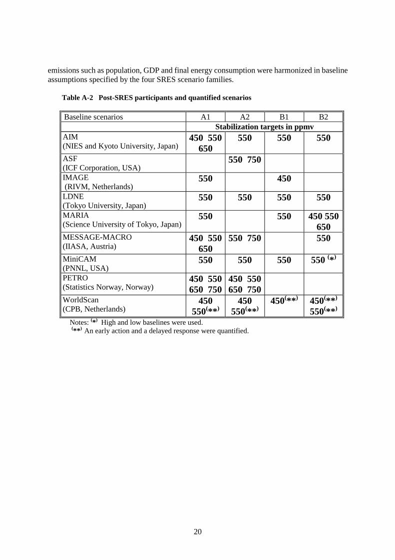
Appendix 2. Outline of Post-SRES Scenarios The new mitigation and stabilization scenarios developed in the Post-SRES effort are based on the four SRES scenario families as baselines. A “Call for Scenarios” was sent by the authors of this paper to more than one hundred researchers in March 1999, and modelers from around the world were invited to prepare quantified stabilization scenarios for two or more concentration levels of atmospheric CO2 in the year 2150, based on one or more of the four SRES scenario families. Alternative concentration ceilings include 450, 550 (minimum requirement), 650, and 750 ppmv, and harmonization with the SRES scenarios was required by tuning reference cases to SRES GDP, population and final energy trajectories. Responding to the call, nine modeling teams participated in the comparison program, included six modeling teams that originally developed the SRES scenarios and three other teams: the AIM team (see article by Jiang, Morita, Masui & Matsuoka in this special issue), the ASF team (see article by Sankovski, Barbour & Pepperin this special issue), the IMAGE team, LDNE team (Yamaji, Fujino & Osada), the MESSAGE-MACRO team (Riahi & Roehrl), the MARIA team (Mori), the MiniCAM team (Pitcher), the PETRO team (Kverndokk, Lindhot & Rosendahl) and the WorldScan team (Bollen, Manders & Timmer). The analyses of eight of these teams are summarized elsewhere in this Special Report Table A-2 shows all the modeling teams and stabilized concentration levels, which were adopted as stabilization targets by each modeling team. Most of the modeling teams analysed more than two SRES baseline scenarios, and half of them analysed more than one stabilization case for at least one of these baselines. This allows a systematic review to be conducted to clarify the relationship between baseline scenarios and mitigation policies/technologies. In total, fifty 1 Post-SRES scenarios were analysed by the nine modeling teams. Because of time constraints, the modeling teams focused their analyses mostly on the energy-related CO2 emissions. However, half of the modeling teams, including AIM, IMAGE, MARIA and MiniCAM, have also tried to quantify mitigation scenarios in non-energy CO2 emissions. The modeling teams that did not estimate non-energy CO2 emissions, introduced exogenous scenarios for these emissions from outside of their models. In order to check the performance of CO2 concentration stabilization for each post-SRES mitigation scenario, a special “generator” (Matsuoka, in this Special Issue) was used by the modeling teams to convert the CO2 emission into CO2 concentrations trajectories. , In addition, the generator was used by them to estimate the eventual level of atmospheric CO2 concentration by 2300 based on the 1990 to 2100 CO2 emissions trajectories from the scenarios This generator is based on the Bern Carbon Cycle Model (Joos et al 1996), which was used in the IPCC Second Assessment Report (IPCC 1995). Using this generator, each modeling team adjusted their mitigation scenarios so that the interpolated CO2 concentration reach one of the alternative fixed target level at 2150 year within 5% error. Further constraint was that the interpolated emission curve should be smooth also after 2100, the end of the time-horizon of the scenarios. This adjustment played an important role in the post-SRES for harmonizing emissions concentrations levels across the stabilization scenarios. The key driving forces of

1Forty-four scenarios are listed on Table 2, but the MiniCAM team quantified two mitigation scenarios for B2-550 ppmv and the WorldScan team did also two scenarios for A1-550, A2-550, B1-450, B2-450 and B2-550 ppmv.

20

emissions such as population, GDP and final energy consumption were harmonized in baseline assumptions specified by the four SRES scenario families.

Table A-2 Post-SRES participants and quantified scenarios

Baseline scenarios A1 A2 B1 B2 Stabilization targets in ppmv AIM (NIES and Kyoto University, Japan)

450 550 650

550 550 550

ASF (ICF Corporation, USA)

550 750

IMAGE (RIVM, Netherlands)

550 450

LDNE (Tokyo University, Japan)

550 550 550 550

MARIA (Science University of Tokyo, Japan)

550 550 450 550 650

MESSAGE-MACRO (IIASA, Austria)

450 550 650

550 750 550

MiniCAM (PNNL, USA)

550 550 550 550 (*)

PETRO (Statistics Norway, Norway)

450 550 650 750

450 550 650 750

WorldScan (CPB, Netherlands)

450 550(**)

450 550(**)

450(**) 450(**) 550(**)

Notes: (*) High and low baselines were used. (**) An early action and a delayed response were quantified.

21

Acknowledgements

The Authors would like to thank all the participants in post-SRES program for their

tremendous efforts in such short period. We also greatly appreciate the very important advice

on the program design provided by Jae Edmons and Rob Swart. This program is supported by

the Global Environmental Research Program of the Japan Environment Agency.

References Alcamo, J., Bouwman, A., Edmonds, J., Gruebler, A., Morita, T., Sugandhy, A (1995) An Evaluation of the IPCC IS92 Emission Scenarios. In Climate Change 1994, Radiative Forcing of Climate Change and An Evaluation of the IPCC IS92 Emission Scenarios. Cambridge University Press. Bollen J., Manders T., Timmer H. (2000) The Benefits and Costs of Waiting--Early action versus delayed response in the post-SRES stabilization scenarios. Special Issue: "Long-term Scenarios on Socioeconomic Development and Climatic Policies," Environmental Economics and Policy Studies, 4 (2). IPCC (1990): Report of the Expert Group on Emission Scenarios. IPCC (1995) Climate Change, The Science of Climate Change, Contribution of Working Group 1 to the Second Assessment Report of the Intergovernmental Panel on Climate Change. Cambridge University Press. Jiang K., Morita T., Masui T., Matsuoka Y. (2000) Global Long-Term GHG Mitigation Emission Scenarios Based on AIM. Special Issue: "Long-term Scenarios on Socioeconomic Development and Climatic Policies," Environmental Economics and Policy Studies, 4 (2). Joos F. et al. (1996) An efficient and accurate representation of complex oceanic and biospheric models of anthropogenic carbon uptake. Tellus, 48B, 389-417. Kverndokk S., Lindholt L., Rosendahl K.E. (2000) Stabilization of CO2 concentrations: Mitigation scenarios using the Petro model. Special Issue: "Long-term Scenarios on Socioeconomic Development and Climatic Policies," Environmental Economics and Policy Studies, 4 (2). Legett, J., Pepper, W., Swart, R (1992): Emission Scenarios for IPCC: An Update. In Climate Change 1992, Supplementary Report to the IPCC Scientific Assessment, Houghton, J., Callander, B, Varney, S. (eds), Cambridge University Press. Matsuoka Y. (2000) Development of a Stabilization Scenario Generator for Long-Term Climatic Assessment. Special Issue: "Long-term Scenarios on Socioeconomic Development and Climatic Policies," Environmental Economics and Policy Studies, 4 (2). Mori S. (2000) Effects of Carbon Emission Mitigation Options under Carbon Concentration Stabilization Scenarios. Special Issue: "Long-term Scenarios on Socioeconomic Development and Climatic Policies," Environmental Economics and Policy Studies, 4 (2).

22

Morita, T., N. Nakicenovic and J. Robinson (2000) Overview of Mitigation Scenarios for Global Climate Stabilization based on New IPCC Emission Scenarios (SRES), Environmental Economics and Policy Studies, 3(2). Nakicenovic, N. et al. (IPCC) (2000): Special Report on Emission Scenarios. Cambridge University Press, 599 pp. Pitcher H. (2000) An Assessment of Mitigation Options in a Sustainable Development World. Special Issue: "Long-term Scenarios on Socioeconomic Development and Climatic Policies," Environmental Economics and Policy Studies, 4 (2). Rana A., Morita T. (2000) Scenarios for Greenhouse Gas Emissions Mitigation: A Review of Modeling of Strategies and Policies in Integrated Assessment Models. Special Issue: "Long-term Scenarios on Socioeconomic Development and Climatic Policies," Environmental Economics and Policy Studies, 4 (2). Riahi K., Roehrl R.A. (2000) Robust Energy Technology Strategies for the 21st Century--Carbon dioxide mitigation and sustainable development. Special Issue: "Long-term Scenarios on Socioeconomic Development and Climatic Policies," Environmental Economics and Policy Studies, 4 (2). Sankovski A., Barbour W., Pepper W. (2000) Climate Change Mitigation in the Regionalized World. Special Issue: "Long-term Scenarios on Socioeconomic Development and Climatic Policies," Environmental Economics and Policy Studies, 4 (2). Yamaji K., Fujino J., Osada K. (2000) Global Energy System to Maintain Atmospheric CO2 Concentration at 550 ppm. Special Issue: "Long-term Scenarios on Socioeconomic Development and Climatic Policies," Environmental Economics and Policy Studies, 4 (2).

23

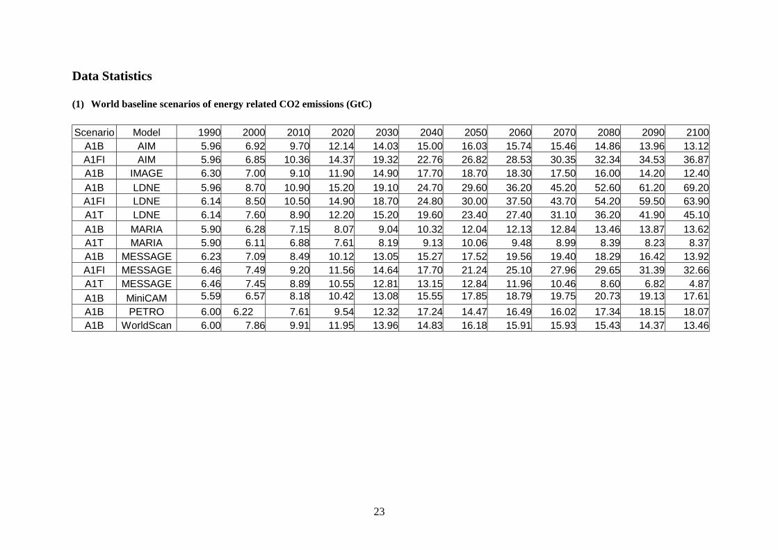
Data Statistics (1) World baseline scenarios of energy related CO2 emissions (GtC) Scenario Model 1990 2000 2010 2020 2030 2040 2050 2060 2070 2080 2090 2100

A1B AIM 5.96 6.92 9.70 12.14 14.03 15.00 16.03 15.74 15.46 14.86 13.96 13.12 A1FI AIM 5.96 6.85 10.36 14.37 19.32 22.76 26.82 28.53 30.35 32.34 34.53 36.87 A1B IMAGE 6.30 7.00 9.10 11.90 14.90 17.70 18.70 18.30 17.50 16.00 14.20 12.40 A1B LDNE 5.96 8.70 10.90 15.20 19.10 24.70 29.60 36.20 45.20 52.60 61.20 69.20 A1FI LDNE 6.14 8.50 10.50 14.90 18.70 24.80 30.00 37.50 43.70 54.20 59.50 63.90 A1T LDNE 6.14 7.60 8.90 12.20 15.20 19.60 23.40 27.40 31.10 36.20 41.90 45.10 A1B MARIA 5.90 6.28 7.15 8.07 9.04 10.32 12.04 12.13 12.84 13.46 13.87 13.62 A1T MARIA 5.90 6.11 6.88 7.61 8.19 9.13 10.06 9.48 8.99 8.39 8.23 8.37 A1B MESSAGE 6.23 7.09 8.49 10.12 13.05 15.27 17.52 19.56 19.40 18.29 16.42 13.92 A1FI MESSAGE 6.46 7.49 9.20 11.56 14.64 17.70 21.24 25.10 27.96 29.65 31.39 32.66 A1T MESSAGE 6.46 7.45 8.89 10.55 12.81 13.15 12.84 11.96 10.46 8.60 6.82 4.87 A1B MiniCAM 5.59 6.57 8.18 10.42 13.08 15.55 17.85 18.79 19.75 20.73 19.13 17.61 A1B PETRO 6.00 6.22 7.61 9.54 12.32 17.24 14.47 16.49 16.02 17.34 18.15 18.07 A1B WorldScan 6.00 7.86 9.91 11.95 13.96 14.83 16.18 15.91 15.93 15.43 14.37 13.46

24

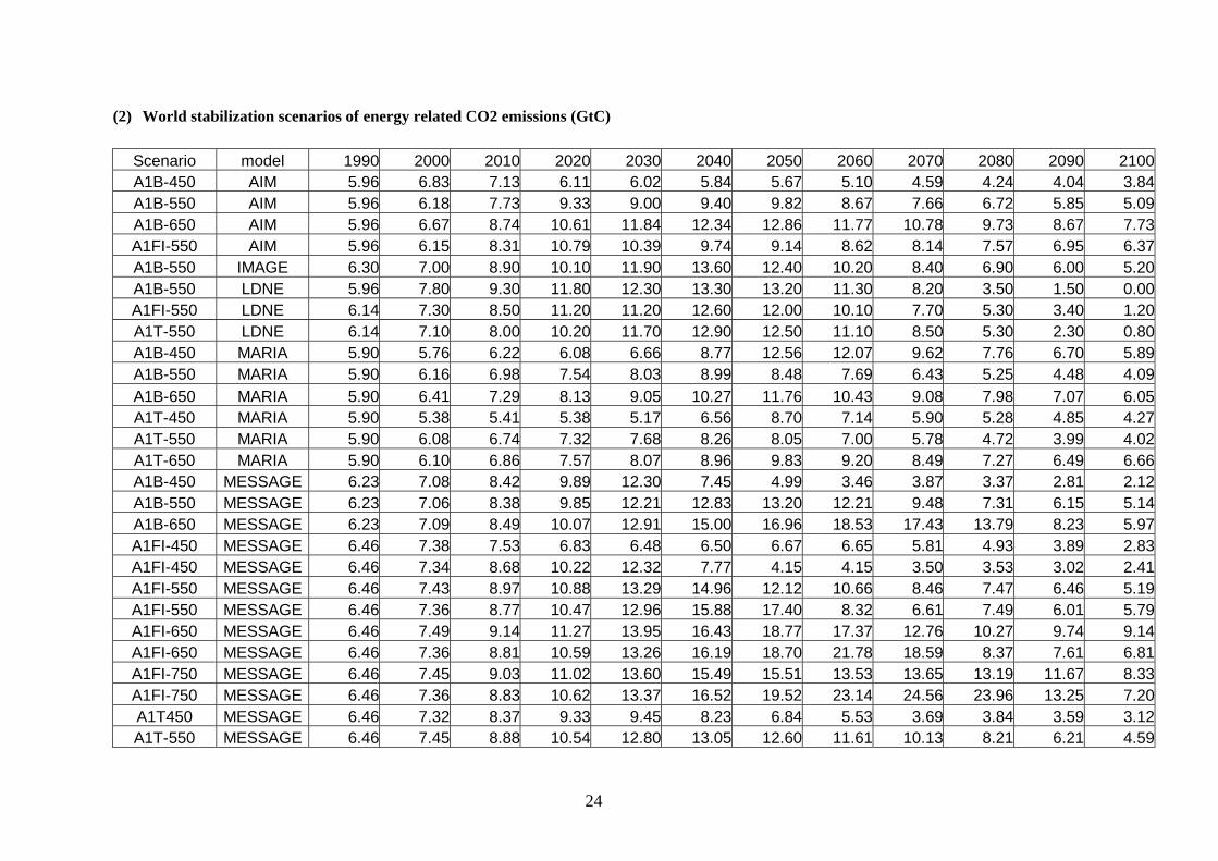
(2) World stabilization scenarios of energy related CO2 emissions (GtC)

Scenario model 1990 2000 2010 2020 2030 2040 2050 2060 2070 2080 2090 2100 A1B-450 AIM 5.96 6.83 7.13 6.11 6.02 5.84 5.67 5.10 4.59 4.24 4.04 3.84 A1B-550 AIM 5.96 6.18 7.73 9.33 9.00 9.40 9.82 8.67 7.66 6.72 5.85 5.09 A1B-650 AIM 5.96 6.67 8.74 10.61 11.84 12.34 12.86 11.77 10.78 9.73 8.67 7.73 A1FI-550 AIM 5.96 6.15 8.31 10.79 10.39 9.74 9.14 8.62 8.14 7.57 6.95 6.37 A1B-550 IMAGE 6.30 7.00 8.90 10.10 11.90 13.60 12.40 10.20 8.40 6.90 6.00 5.20 A1B-550 LDNE 5.96 7.80 9.30 11.80 12.30 13.30 13.20 11.30 8.20 3.50 1.50 0.00 A1FI-550 LDNE 6.14 7.30 8.50 11.20 11.20 12.60 12.00 10.10 7.70 5.30 3.40 1.20 A1T-550 LDNE 6.14 7.10 8.00 10.20 11.70 12.90 12.50 11.10 8.50 5.30 2.30 0.80 A1B-450 MARIA 5.90 5.76 6.22 6.08 6.66 8.77 12.56 12.07 9.62 7.76 6.70 5.89 A1B-550 MARIA 5.90 6.16 6.98 7.54 8.03 8.99 8.48 7.69 6.43 5.25 4.48 4.09 A1B-650 MARIA 5.90 6.41 7.29 8.13 9.05 10.27 11.76 10.43 9.08 7.98 7.07 6.05 A1T-450 MARIA 5.90 5.38 5.41 5.38 5.17 6.56 8.70 7.14 5.90 5.28 4.85 4.27 A1T-550 MARIA 5.90 6.08 6.74 7.32 7.68 8.26 8.05 7.00 5.78 4.72 3.99 4.02 A1T-650 MARIA 5.90 6.10 6.86 7.57 8.07 8.96 9.83 9.20 8.49 7.27 6.49 6.66 A1B-450 MESSAGE 6.23 7.08 8.42 9.89 12.30 7.45 4.99 3.46 3.87 3.37 2.81 2.12 A1B-550 MESSAGE 6.23 7.06 8.38 9.85 12.21 12.83 13.20 12.21 9.48 7.31 6.15 5.14 A1B-650 MESSAGE 6.23 7.09 8.49 10.07 12.91 15.00 16.96 18.53 17.43 13.79 8.23 5.97 A1FI-450 MESSAGE 6.46 7.38 7.53 6.83 6.48 6.50 6.67 6.65 5.81 4.93 3.89 2.83 A1FI-450 MESSAGE 6.46 7.34 8.68 10.22 12.32 7.77 4.15 4.15 3.50 3.53 3.02 2.41 A1FI-550 MESSAGE 6.46 7.43 8.97 10.88 13.29 14.96 12.12 10.66 8.46 7.47 6.46 5.19 A1FI-550 MESSAGE 6.46 7.36 8.77 10.47 12.96 15.88 17.40 8.32 6.61 7.49 6.01 5.79 A1FI-650 MESSAGE 6.46 7.49 9.14 11.27 13.95 16.43 18.77 17.37 12.76 10.27 9.74 9.14 A1FI-650 MESSAGE 6.46 7.36 8.81 10.59 13.26 16.19 18.70 21.78 18.59 8.37 7.61 6.81 A1FI-750 MESSAGE 6.46 7.45 9.03 11.02 13.60 15.49 15.51 13.53 13.65 13.19 11.67 8.33 A1FI-750 MESSAGE 6.46 7.36 8.83 10.62 13.37 16.52 19.52 23.14 24.56 23.96 13.25 7.20 A1T450 MESSAGE 6.46 7.32 8.37 9.33 9.45 8.23 6.84 5.53 3.69 3.84 3.59 3.12 A1T-550 MESSAGE 6.46 7.45 8.88 10.54 12.80 13.05 12.60 11.61 10.13 8.21 6.21 4.59

25

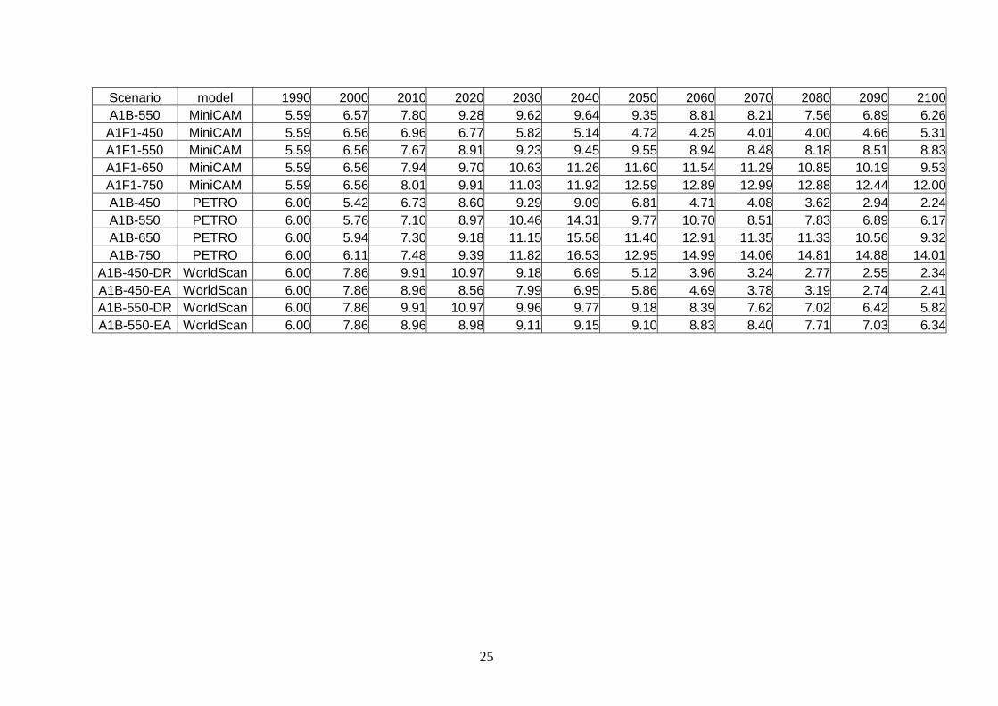
Scenario model 1990 2000 2010 2020 2030 2040 2050 2060 2070 2080 2090 2100 A1B-550 MiniCAM 5.59 6.57 7.80 9.28 9.62 9.64 9.35 8.81 8.21 7.56 6.89 6.26 A1F1-450 MiniCAM 5.59 6.56 6.96 6.77 5.82 5.14 4.72 4.25 4.01 4.00 4.66 5.31 A1F1-550 MiniCAM 5.59 6.56 7.67 8.91 9.23 9.45 9.55 8.94 8.48 8.18 8.51 8.83 A1F1-650 MiniCAM 5.59 6.56 7.94 9.70 10.63 11.26 11.60 11.54 11.29 10.85 10.19 9.53 A1F1-750 MiniCAM 5.59 6.56 8.01 9.91 11.03 11.92 12.59 12.89 12.99 12.88 12.44 12.00 A1B-450 PETRO 6.00 5.42 6.73 8.60 9.29 9.09 6.81 4.71 4.08 3.62 2.94 2.24 A1B-550 PETRO 6.00 5.76 7.10 8.97 10.46 14.31 9.77 10.70 8.51 7.83 6.89 6.17 A1B-650 PETRO 6.00 5.94 7.30 9.18 11.15 15.58 11.40 12.91 11.35 11.33 10.56 9.32 A1B-750 PETRO 6.00 6.11 7.48 9.39 11.82 16.53 12.95 14.99 14.06 14.81 14.88 14.01

A1B-450-DR WorldScan 6.00 7.86 9.91 10.97 9.18 6.69 5.12 3.96 3.24 2.77 2.55 2.34 A1B-450-EA WorldScan 6.00 7.86 8.96 8.56 7.99 6.95 5.86 4.69 3.78 3.19 2.74 2.41 A1B-550-DR WorldScan 6.00 7.86 9.91 10.97 9.96 9.77 9.18 8.39 7.62 7.02 6.42 5.82 A1B-550-EA WorldScan 6.00 7.86 8.96 8.98 9.11 9.15 9.10 8.83 8.40 7.71 7.03 6.34

26

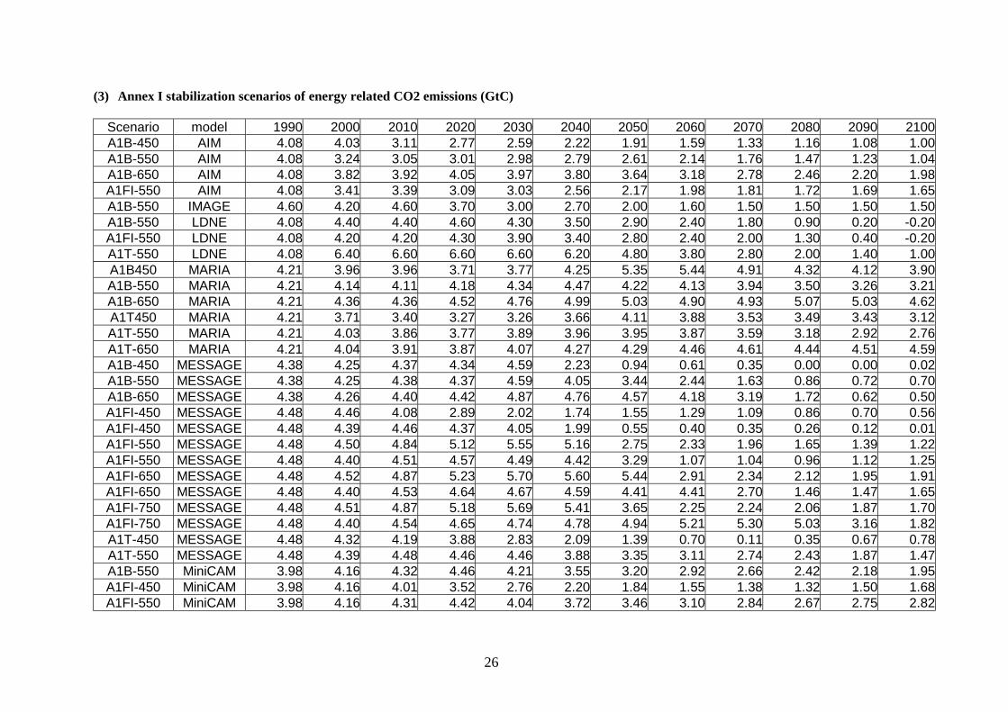
(3) Annex I stabilization scenarios of energy related CO2 emissions (GtC)

Scenario model 1990 2000 2010 2020 2030 2040 2050 2060 2070 2080 2090 2100 A1B-450 AIM 4.08 4.03 3.11 2.77 2.59 2.22 1.91 1.59 1.33 1.16 1.08 1.00 A1B-550 AIM 4.08 3.24 3.05 3.01 2.98 2.79 2.61 2.14 1.76 1.47 1.23 1.04 A1B-650 AIM 4.08 3.82 3.92 4.05 3.97 3.80 3.64 3.18 2.78 2.46 2.20 1.98 A1FI-550 AIM 4.08 3.41 3.39 3.09 3.03 2.56 2.17 1.98 1.81 1.72 1.69 1.65 A1B-550 IMAGE 4.60 4.20 4.60 3.70 3.00 2.70 2.00 1.60 1.50 1.50 1.50 1.50 A1B-550 LDNE 4.08 4.40 4.40 4.60 4.30 3.50 2.90 2.40 1.80 0.90 0.20 -0.20 A1FI-550 LDNE 4.08 4.20 4.20 4.30 3.90 3.40 2.80 2.40 2.00 1.30 0.40 -0.20 A1T-550 LDNE 4.08 6.40 6.60 6.60 6.60 6.20 4.80 3.80 2.80 2.00 1.40 1.00 A1B450 MARIA 4.21 3.96 3.96 3.71 3.77 4.25 5.35 5.44 4.91 4.32 4.12 3.90 A1B-550 MARIA 4.21 4.14 4.11 4.18 4.34 4.47 4.22 4.13 3.94 3.50 3.26 3.21 A1B-650 MARIA 4.21 4.36 4.36 4.52 4.76 4.99 5.03 4.90 4.93 5.07 5.03 4.62 A1T450 MARIA 4.21 3.71 3.40 3.27 3.26 3.66 4.11 3.88 3.53 3.49 3.43 3.12 A1T-550 MARIA 4.21 4.03 3.86 3.77 3.89 3.96 3.95 3.87 3.59 3.18 2.92 2.76 A1T-650 MARIA 4.21 4.04 3.91 3.87 4.07 4.27 4.29 4.46 4.61 4.44 4.51 4.59 A1B-450 MESSAGE 4.38 4.25 4.37 4.34 4.59 2.23 0.94 0.61 0.35 0.00 0.00 0.02 A1B-550 MESSAGE 4.38 4.25 4.38 4.37 4.59 4.05 3.44 2.44 1.63 0.86 0.72 0.70 A1B-650 MESSAGE 4.38 4.26 4.40 4.42 4.87 4.76 4.57 4.18 3.19 1.72 0.62 0.50 A1FI-450 MESSAGE 4.48 4.46 4.08 2.89 2.02 1.74 1.55 1.29 1.09 0.86 0.70 0.56 A1FI-450 MESSAGE 4.48 4.39 4.46 4.37 4.05 1.99 0.55 0.40 0.35 0.26 0.12 0.01 A1FI-550 MESSAGE 4.48 4.50 4.84 5.12 5.55 5.16 2.75 2.33 1.96 1.65 1.39 1.22 A1FI-550 MESSAGE 4.48 4.40 4.51 4.57 4.49 4.42 3.29 1.07 1.04 0.96 1.12 1.25 A1FI-650 MESSAGE 4.48 4.52 4.87 5.23 5.70 5.60 5.44 2.91 2.34 2.12 1.95 1.91 A1FI-650 MESSAGE 4.48 4.40 4.53 4.64 4.67 4.59 4.41 4.41 2.70 1.46 1.47 1.65 A1FI-750 MESSAGE 4.48 4.51 4.87 5.18 5.69 5.41 3.65 2.25 2.24 2.06 1.87 1.70 A1FI-750 MESSAGE 4.48 4.40 4.54 4.65 4.74 4.78 4.94 5.21 5.30 5.03 3.16 1.82 A1T-450 MESSAGE 4.48 4.32 4.19 3.88 2.83 2.09 1.39 0.70 0.11 0.35 0.67 0.78 A1T-550 MESSAGE 4.48 4.39 4.48 4.46 4.46 3.88 3.35 3.11 2.74 2.43 1.87 1.47 A1B-550 MiniCAM 3.98 4.16 4.32 4.46 4.21 3.55 3.20 2.92 2.66 2.42 2.18 1.95 A1FI-450 MiniCAM 3.98 4.16 4.01 3.52 2.76 2.20 1.84 1.55 1.38 1.32 1.50 1.68 A1FI-550 MiniCAM 3.98 4.16 4.31 4.42 4.04 3.72 3.46 3.10 2.84 2.67 2.75 2.82

27

Scenario model 1990 2000 2010 2020 2030 2040 2050 2060 2070 2080 2090 2100 A1FI-650 MiniCAM 3.98 4.16 4.42 4.75 4.53 4.31 4.11 3.90 3.70 3.51 3.28 3.05 A1FI-750 MiniCAM 3.98 4.16 4.44 4.84 4.67 4.52 4.41 4.30 4.20 4.12 3.98 3.83 A1B-450 PETRO 4.10 3.00 3.27 3.59 4.07 2.03 1.58 0.91 0.74 0.63 0.49 0.36 A1B-550 PETRO 4.10 3.36 3.66 4.00 4.47 5.07 2.29 2.06 1.60 1.38 1.15 0.98 A1B-650 PETRO 4.10 3.54 3.87 4.23 4.71 5.64 2.70 2.55 2.17 2.04 1.78 1.48 A1B-750 PETRO 4.10 3.70 4.05 4.45 4.95 5.92 3.09 3.02 2.74 2.71 2.56 2.26


28

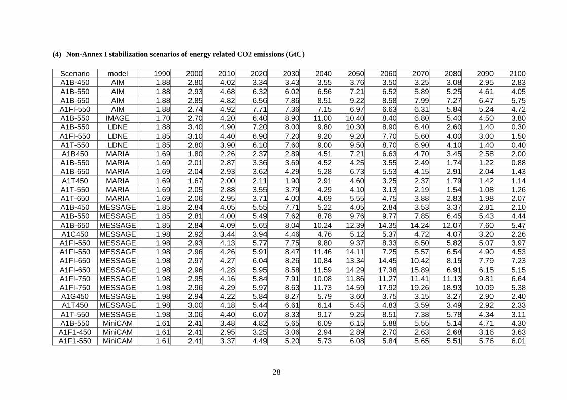
(4) Non-Annex I stabilization scenarios of energy related CO2 emissions (GtC)

Scenario model 1990 2000 2010 2020 2030 2040 2050 2060 2070 2080 2090 2100 A1B-450 AIM 1.88 2.80 4.02 3.34 3.43 3.55 3.76 3.50 3.25 3.08 2.95 2.83 A1B-550 AIM 1.88 2.93 4.68 6.32 6.02 6.56 7.21 6.52 5.89 5.25 4.61 4.05 A1B-650 AIM 1.88 2.85 4.82 6.56 7.86 8.51 9.22 8.58 7.99 7.27 6.47 5.75 A1FI-550 AIM 1.88 2.74 4.92 7.71 7.36 7.15 6.97 6.63 6.31 5.84 5.24 4.72 A1B-550 IMAGE 1.70 2.70 4.20 6.40 8.90 11.00 10.40 8.40 6.80 5.40 4.50 3.80 A1B-550 LDNE 1.88 3.40 4.90 7.20 8.00 9.80 10.30 8.90 6.40 2.60 1.40 0.30 A1FI-550 LDNE 1.85 3.10 4.40 6.90 7.20 9.20 9.20 7.70 5.60 4.00 3.00 1.50 A1T-550 LDNE 1.85 2.80 3.90 6.10 7.60 9.00 9.50 8.70 6.90 4.10 1.40 0.40 A1B450 MARIA 1.69 1.80 2.26 2.37 2.89 4.51 7.21 6.63 4.70 3.45 2.58 2.00 A1B-550 MARIA 1.69 2.01 2.87 3.36 3.69 4.52 4.25 3.55 2.49 1.74 1.22 0.88 A1B-650 MARIA 1.69 2.04 2.93 3.62 4.29 5.28 6.73 5.53 4.15 2.91 2.04 1.43 A1T450 MARIA 1.69 1.67 2.00 2.11 1.90 2.91 4.60 3.25 2.37 1.79 1.42 1.14 A1T-550 MARIA 1.69 2.05 2.88 3.55 3.79 4.29 4.10 3.13 2.19 1.54 1.08 1.26 A1T-650 MARIA 1.69 2.06 2.95 3.71 4.00 4.69 5.55 4.75 3.88 2.83 1.98 2.07 A1B-450 MESSAGE 1.85 2.84 4.05 5.55 7.71 5.22 4.05 2.84 3.53 3.37 2.81 2.10 A1B-550 MESSAGE 1.85 2.81 4.00 5.49 7.62 8.78 9.76 9.77 7.85 6.45 5.43 4.44 A1B-650 MESSAGE 1.85 2.84 4.09 5.65 8.04 10.24 12.39 14.35 14.24 12.07 7.60 5.47 A1C450 MESSAGE 1.98 2.92 3.44 3.94 4.46 4.76 5.12 5.37 4.72 4.07 3.20 2.26 A1FI-550 MESSAGE 1.98 2.93 4.13 5.77 7.75 9.80 9.37 8.33 6.50 5.82 5.07 3.97 A1FI-550 MESSAGE 1.98 2.96 4.26 5.91 8.47 11.46 14.11 7.25 5.57 6.54 4.90 4.53 A1FI-650 MESSAGE 1.98 2.97 4.27 6.04 8.26 10.84 13.34 14.45 10.42 8.15 7.79 7.23 A1FI-650 MESSAGE 1.98 2.96 4.28 5.95 8.58 11.59 14.29 17.38 15.89 6.91 6.15 5.15 A1FI-750 MESSAGE 1.98 2.95 4.16 5.84 7.91 10.08 11.86 11.27 11.41 11.13 9.81 6.64 A1FI-750 MESSAGE 1.98 2.96 4.29 5.97 8.63 11.73 14.59 17.92 19.26 18.93 10.09 5.38 A1G450 MESSAGE 1.98 2.94 4.22 5.84 8.27 5.79 3.60 3.75 3.15 3.27 2.90 2.40 A1T450 MESSAGE 1.98 3.00 4.18 5.44 6.61 6.14 5.45 4.83 3.59 3.49 2.92 2.33 A1T-550 MESSAGE 1.98 3.06 4.40 6.07 8.33 9.17 9.25 8.51 7.38 5.78 4.34 3.11 A1B-550 MiniCAM 1.61 2.41 3.48 4.82 5.65 6.09 6.15 5.88 5.55 5.14 4.71 4.30 A1F1-450 MiniCAM 1.61 2.41 2.95 3.25 3.06 2.94 2.89 2.70 2.63 2.68 3.16 3.63 A1F1-550 MiniCAM 1.61 2.41 3.37 4.49 5.20 5.73 6.08 5.84 5.65 5.51 5.76 6.01

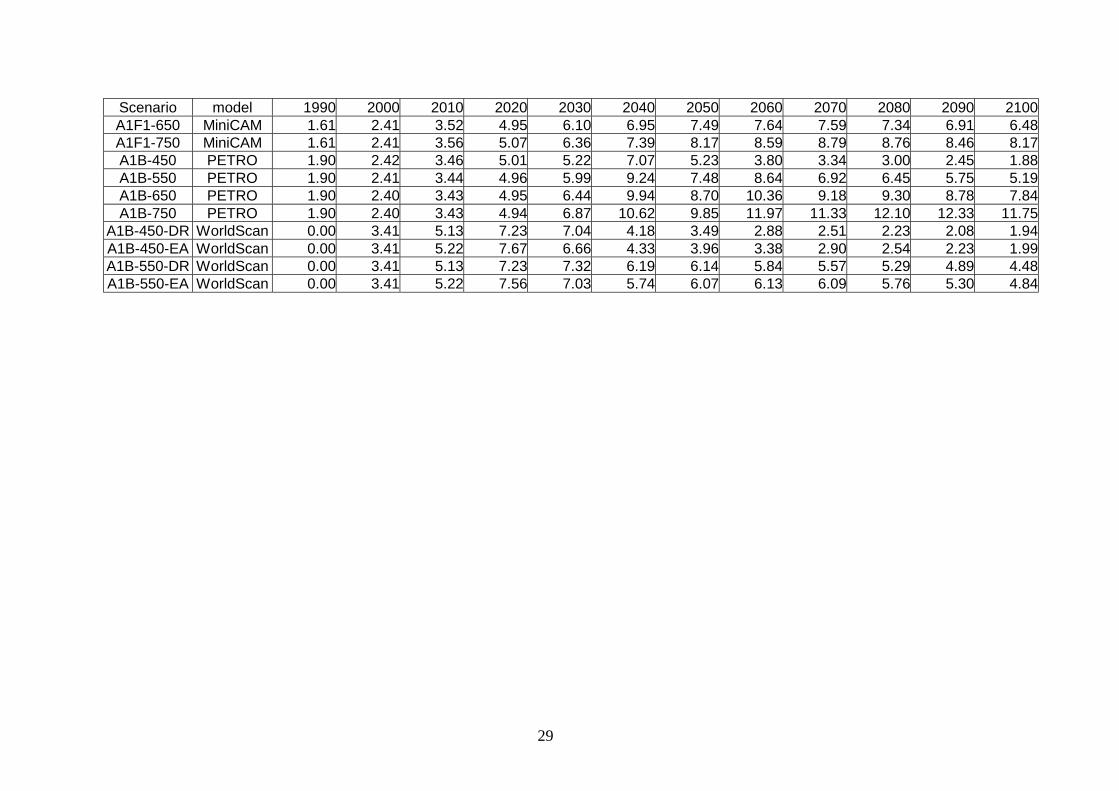
29

Scenario model 1990 2000 2010 2020 2030 2040 2050 2060 2070 2080 2090 2100 A1F1-650 MiniCAM 1.61 2.41 3.52 4.95 6.10 6.95 7.49 7.64 7.59 7.34 6.91 6.48 A1F1-750 MiniCAM 1.61 2.41 3.56 5.07 6.36 7.39 8.17 8.59 8.79 8.76 8.46 8.17 A1B-450 PETRO 1.90 2.42 3.46 5.01 5.22 7.07 5.23 3.80 3.34 3.00 2.45 1.88 A1B-550 PETRO 1.90 2.41 3.44 4.96 5.99 9.24 7.48 8.64 6.92 6.45 5.75 5.19 A1B-650 PETRO 1.90 2.40 3.43 4.95 6.44 9.94 8.70 10.36 9.18 9.30 8.78 7.84 A1B-750 PETRO 1.90 2.40 3.43 4.94 6.87 10.62 9.85 11.97 11.33 12.10 12.33 11.75


the relationship between technological development paths and the

Documents