the queen’s tower imperial college london south kensington, sw7 28th jan 2007 | ashley brown...

The Queen’s TowerThe Queen’s TowerImperial College LondonImperial College LondonSouth Kensington, SW7South Kensington, SW7

28th Jan 2007 | Ashley Brown

Profiling floating point Profiling floating point value ranges for value ranges for reconfigurable reconfigurable

implementationimplementation

Workshop on Reconfigurable Computing at 2007

Ashley Brown, 28th Jan 2007

28th Jan 2007 | Ashley Brown # 2

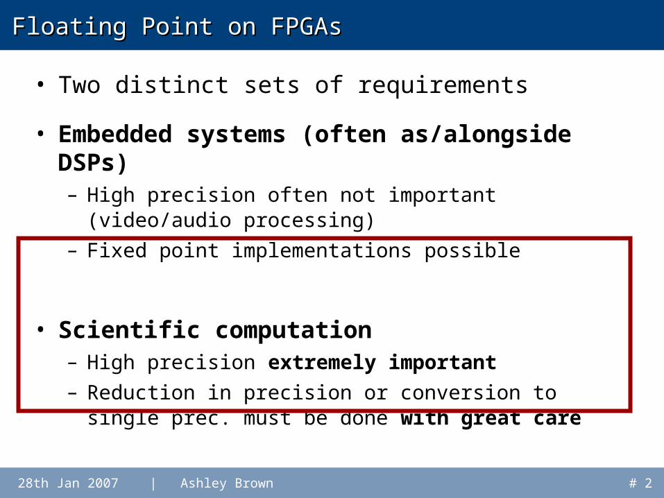
Floating Point on FPGAsFloating Point on FPGAs

• Two distinct sets of requirements

• Embedded systems (often as/alongside DSPs)– High precision often not important (video/audio

processing)– Fixed point implementations possible

• Scientific computation– High precision extremely important– Reduction in precision or conversion to single prec.

must be done with great care


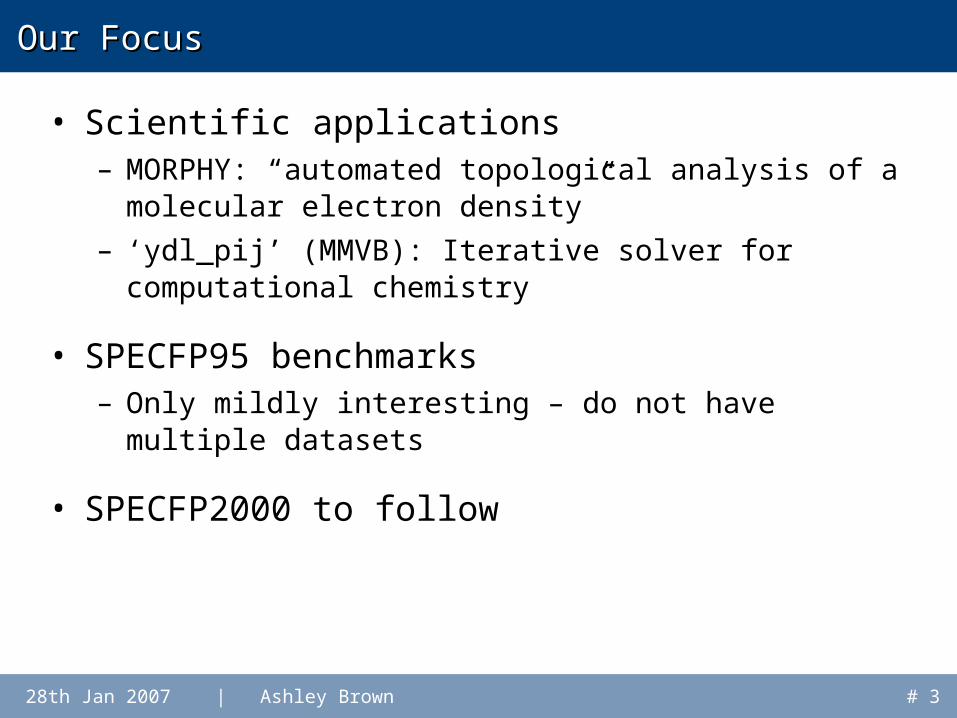
Our FocusOur Focus

• Scientific applications– MORPHY: “automated topological analysis of a

molecular electron density”– ‘ydl_pij’ (MMVB): Iterative solver for computational

chemistry

• SPECFP95 benchmarks– Only mildly interesting – do not have multiple

datasets

• SPECFP2000 to follow


The ProblemThe Problem

• D.P. floating point on FPGAs uses a lot of area

• Density is improving: but still want to squeeze more in!– Re-using hardware can reduce concurrency

• Scientific applications: typically 64-bit floating point

• Often full precision is (believed to be) required– Is this really the case?

• We have more options than single or double


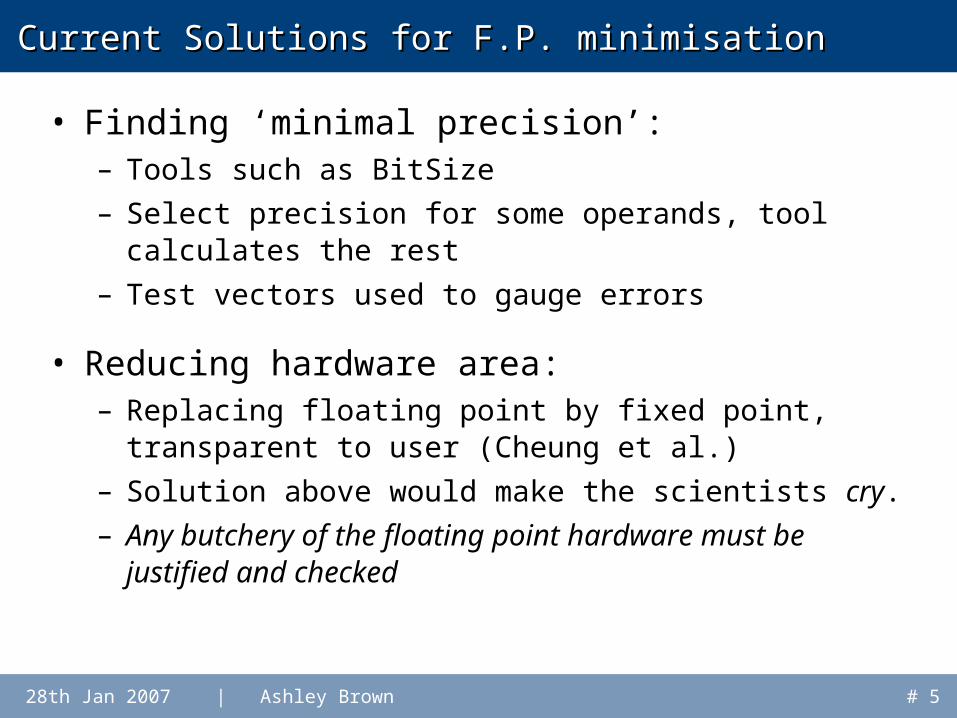
Current Solutions for F.P. minimisationCurrent Solutions for F.P. minimisation

• Finding ‘minimal precision’:– Tools such as BitSize– Select precision for some operands, tool calculates

the rest– Test vectors used to gauge errors

• Reducing hardware area:– Replacing floating point by fixed point, transparent

to user (Cheung et al.)– Solution above would make the scientists cry.– Any butchery of the floating point hardware must be

justified and checked


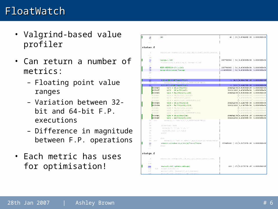
FloatWatchFloatWatch

• Valgrind-based value profiler

• Can return a number of metrics:– Floating point value

ranges– Variation between 32-bit

and 64-bit F.P. executions

– Difference in magnitude between F.P. operations

• Each metric has uses for optimisation!


0

50000000

100000000

150000000

200000000

250000000

300000000

Value Magnitude

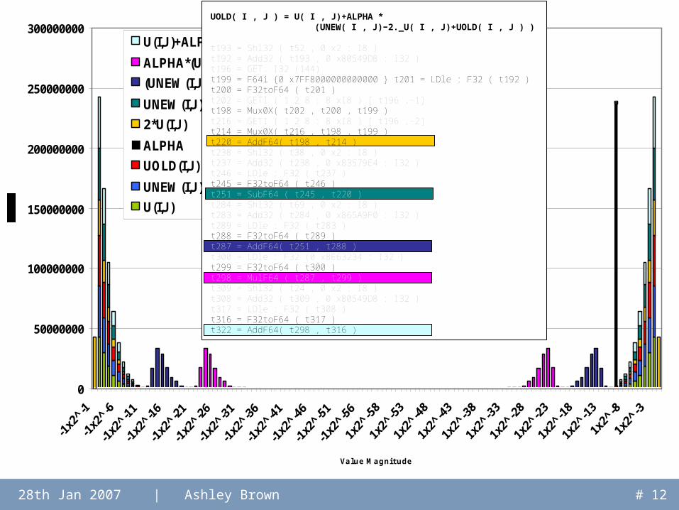
U(I,J)+ALPHA*(UNEW(I,J)-2.*U(I,J)+UOLD(I,J))

ALPHA*(UNEW(I,J)-2.*U(I,J)+UOLD(I,J))

(UNEW(I,J)-2.*U(I,J)+UOLD(I,J))

UNEW(I,J)-2.*U(I,J)

2*U(I,J)

ALPHA

UOLD(I,J)

UNEW(I,J)

U(I,J)

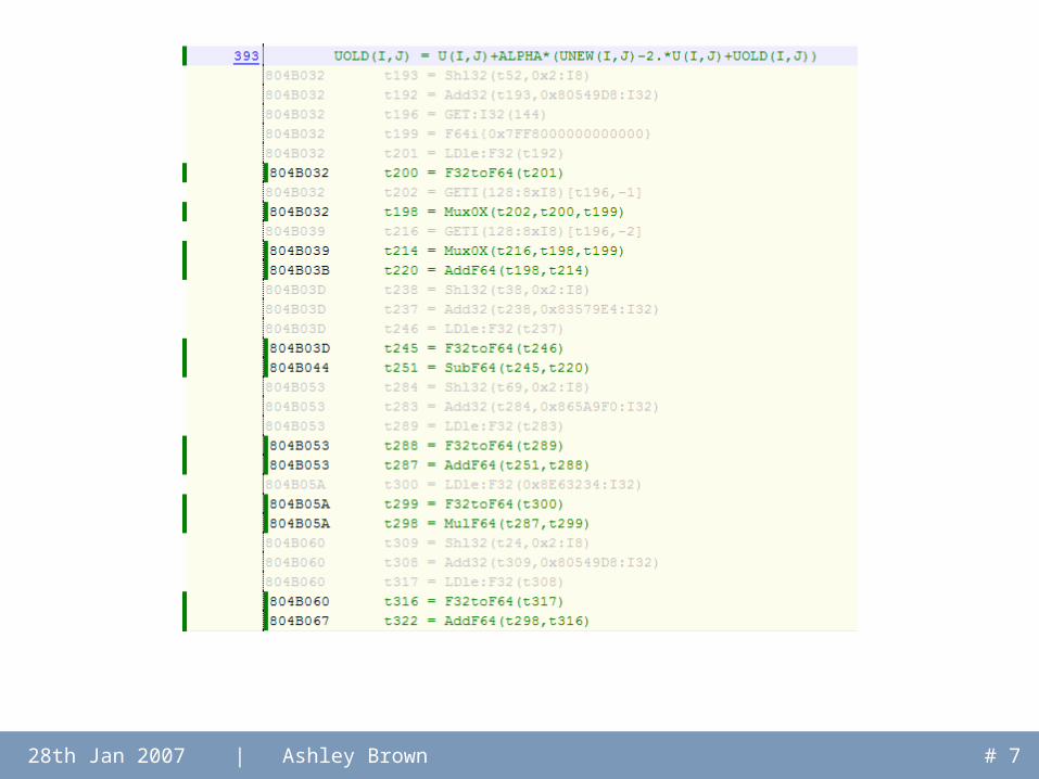
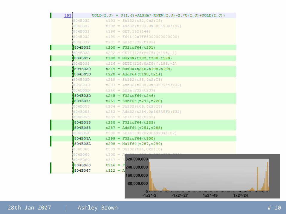
UOLD( I , J ) = U( I , J )+ALPHA * (UNEW( I , J )−2. _U( I , J )+UOLD( I , J ) )

t 193 = Shl 32 ( t 52 , 0 x2 : I 8 )t 192 = Add32 ( t 193 , 0 x80549D8 : I 32 )t 196 = GET: I 32 ( 144)t 199 = F64i {0 x7FF8000000000000 } t 201 = LDl e : F32 ( t 192 )t 200 = F32t oF64 ( t 201 )t 202 = GETI ( 1 2 8 : 8 xI 8 ) [ t 196 , −1]t 198 = Mux0X( t 202 , t 200 , t 199 )t 216 = GETI ( 1 2 8 : 8 xI 8 ) [ t 196 , −2]t 214 = Mux0X( t 216 , t 198 , t 199 )t 220 = AddF64( t 198 , t 214 )t 238 = Shl 32 ( t 38 , 0 x2 : I 8 )t 237 = Add32 ( t 238 , 0 x83579E4 : I 32 )t 246 = LDl e : F32 ( t 237 )t 245 = F32t oF64 ( t 246 )t 251 = SubF64 ( t 245 , t 220 )t 284 = Shl 32 ( t 69 , 0 x2 : I 8 )t 283 = Add32 ( t 284 , 0 x865A9F0 : I 32 )t 289 = LDl e : F32 ( t 283 )t 288 = F32t oF64 ( t 289 )t 287 = AddF64( t 251 , t 288 )t 300 = LDl e : F32 ( 0 x8E63234 : I 32 )t 299 = F32t oF64 ( t 300 )t 298 = Mul F64 ( t 287 , t 299 )t 309 = Shl 32 ( t 24 , 0 x2 : I 8 )t 308 = Add32 ( t 309 , 0 x80549D8 : I 32 )t 317 = LDl e : F32 ( t 308 )t 316 = F32t oF64 ( t 317 )t 322 = AddF64( t 298 , t 316 )


What does this tell us?What does this tell us?

• Alpha is constant (but could have found that from source)

• Memory operands all fall within the same range

• Result falls within the same range as memory operands

• Intermediate values result in a shift in the range

• Optimisation: we do not need double precision– A custom floating point format would suffice


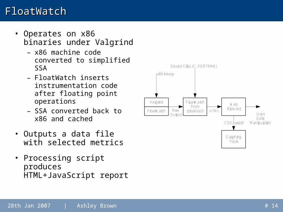
FloatWatchFloatWatch

• Operates on x86 binaries under Valgrind– x86 machine code

converted to simplified SSA

– FloatWatch inserts instrumentation code after floating point operations

– SSA converted back to x86 and cached

• Outputs a data file with selected metrics

• Processing script produces HTML+JavaScript report

Valgrind

FloatWatch

FloatWatchPost-

processorRawOutput

Web Browser

Graphing Tools

UserData

ManipulationCSV export

x86 binary

Source Files (C, FORTRAN)

HTML


ReportReport

• Dynamic HTML interface– Copy HTML file from computing cluster to desktop,

no installation required

• Select/deselect source lines, SSA “instructions”– Dynamic in-page graph – Table for exporting to GNU-plot, Excel etc.

• View value ranges at instruction, source line, function, file and application levels.


Optimisation OpportunitiesOptimisation Opportunities

• Reduce floating point unit– Reduced precision– Restricted normalisation

• Use an alternative representation– Non-standard floating point (e.g. 48-bit)– Fixed point– Dual fixed-point

• Minimisation of redundancy– Remove denormal handling unless required– Remove or predict zero-value calculations


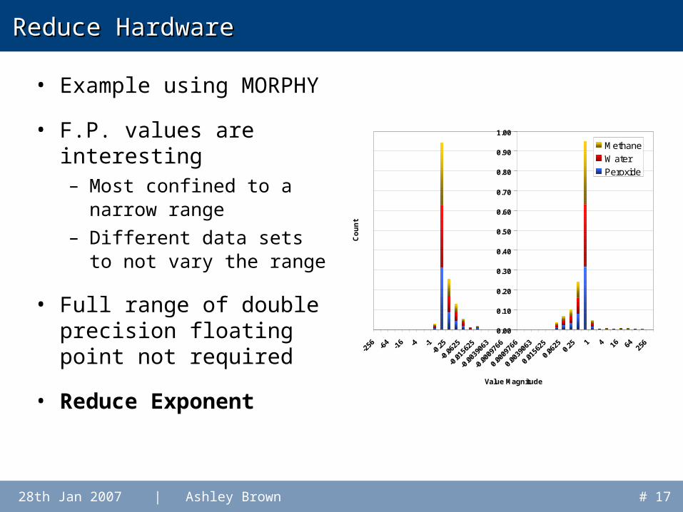
Reduce HardwareReduce Hardware

• Example using MORPHY

• F.P. values are interesting– Most confined to a

narrow range– Different data sets to

not vary the range

• Full range of double precision floating point not required

• Reduce Exponent

0.00

0.10

0.20

0.30

0.40

0.50

0.60

0.70

0.80

0.90

1.00

-256 -6

4-1

6 -4 -1-0

.25

-0.0

625

-0.0

1562

5

-0.0

0390

63

-0.0

0097

66

0.00

0976

6

0.00

3906

3

0.01

5625

0.06

250.

25 1 4 16 64 256

Value Magnitude

Co

un

t

Methane

Water

Peroxide


Reduce Hardware – Alignment/NormalisationReduce Hardware – Alignment/Normalisation

• Most expensive step: shifting for add/subtract– Operand alignment– Normalisation

• Set limits on alignment to reduce hardware size– Trap to software to perform other alignments

• Provisional results: only shift-by-4 required for some applications


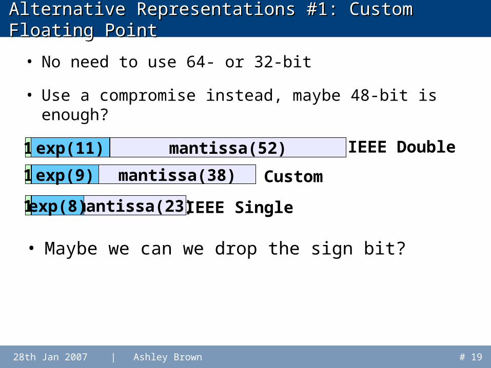
Alternative Representations #1: Custom Floating Alternative Representations #1: Custom Floating PointPoint

• No need to use 64- or 32-bit

• Use a compromise instead, maybe 48-bit is enough?

1 mantissa(52)exp(11)



IEEE Single

Custom

IEEE Double

• Maybe we can we drop the sign bit?


Alternative Representations #2: Fixed PointAlternative Representations #2: Fixed Point

• For very narrow ranges, fixed point may be an option

• Must be treated with extreme care

• Dual fixed-point format provides another possibility– Two different formats: different fixed point positions– 1 bit reserved to switch between formats


““Pipeline Prediction”Pipeline Prediction”

• Similar concept to branch prediction

• Build a selection of pipelines with different performance characteristics– Slow but generic version– Fast version with limited range, reduced operand

alignment– Compromise in between

• Predict which version is best to use (how?)


True Reconfiguration – Temporal ProfilingTrue Reconfiguration – Temporal Profiling

• Value ranges can vary for different application phases

• Potential to reconfigure hardware as phases change

• Test applications have not shown this behaviour so far– Small kernels only– Full applications would be expected to show this

behaviour


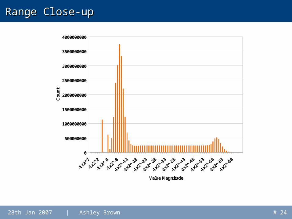
Profiling Results – SPECFP95 ‘mgrid’Profiling Results – SPECFP95 ‘mgrid’

0

500000000

1000000000

1500000000

2000000000

2500000000

3000000000

3500000000

4000000000

-1x

2^

65

-1x

2^

-45

-1x

2^

-15

5

-1x

2^

-26

5

-1x

2^

-37

5

-1x

2^

-48

5

-1x

2^

-59

5

-1x

2^

-70

5

-1x

2^

-81

5

-1x

2^

-92

5

1x

2^

-10

12

1x

2^

-90

2

1x

2^

-79

2

1x

2^

-68

2

1x

2^

-57

2

1x

2^

-46

2

1x

2^

-35

2

1x

2^

-24

2

1x

2^

-13

2

1x

2^

-22

Value Magnitude

Co

un

t

Operations producing zero

Two ranges: similar shapes


Range Close-upRange Close-up

0

500000000

1000000000

1500000000

2000000000

2500000000

3000000000

3500000000

4000000000

-1x2

^7

-1x2

^2

-1x2

^-3

-1x2

^-8

-1x2

^-13

-1x2

^-18

-1x2

^-23

-1x2

^-28

-1x2

^-33

-1x2

^-38

-1x2

^-43

-1x2

^-48

-1x2

^-53

-1x2

^-58

-1x2

^-63

-1x2

^-68

Value Magnitude

Co

un

t


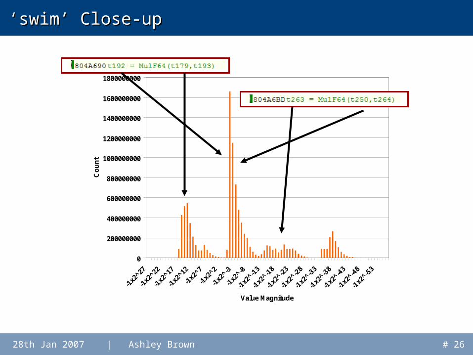
Profiling Results – SPECFP95 ‘swim’Profiling Results – SPECFP95 ‘swim’

0

1000000000

2000000000

3000000000

4000000000

5000000000

6000000000

-1x

2^

47

-1x

2^

26

-1x

2^

5

-1x

2^

-16

-1x

2^

-37

-1x

2^

-58

-1x

2^

-79

-1x

2^

-10

0

-1x

2^

-12

1

-1x

2^

-14

2

1x

2^

-15

4

1x

2^

-13

3

1x

2^

-11

2

1x

2^

-91

1x

2^

-70

1x

2^

-49

1x

2^

-28

1x

2^

-7

1x

2^

14

1x

2^

35

Value Magnitude

Co

un

t

Sawtooth caused by multiplication


‘‘swim’ Close-upswim’ Close-up

0

200000000

400000000

600000000

800000000

1000000000

1200000000

1400000000

1600000000

1800000000

-1x2

^27

-1x2

^22

-1x2

^17

-1x2

^12

-1x2

^7

-1x2

^2

-1x2

^-3

-1x2

^-8

-1x2

^-13

-1x2

^-18

-1x2

^-23

-1x2

^-28

-1x2

^-33

-1x2

^-38

-1x2

^-43

-1x2

^-48

-1x2

^-53

Value Magnitude

Co

un

t


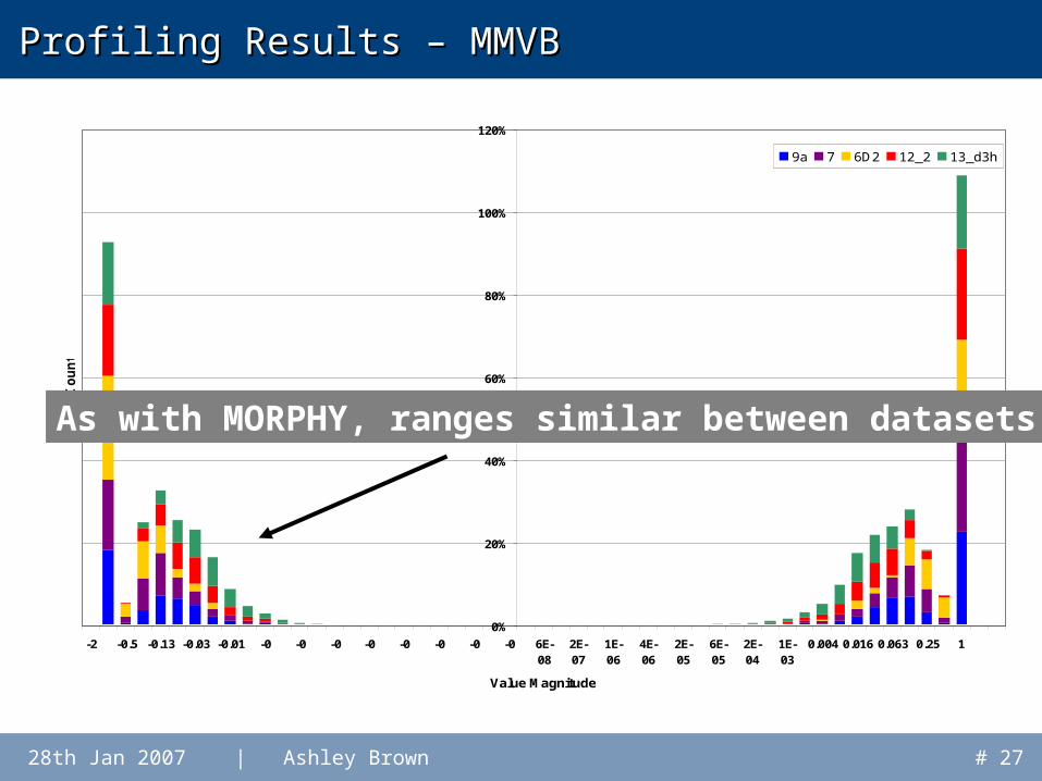
Profiling Results – MMVBProfiling Results – MMVB

0%

20%

40%

60%

80%

100%

120%

-2 -0.5 -0.13 -0.03 -0.01 -0 -0 -0 -0 -0 -0 -0 -0 6E-08

2E-07

1E-06

4E-06

2E-05

6E-05

2E-04

1E-03

0.004 0.016 0.063 0.25 1

Value Magnitude

Co

un

t

9a 7 6D2 12_2 13_d3h

As with MORPHY, ranges similar between datasets


Problems with this approachProblems with this approach

• No guarantees that values do not occur outside identified ranges

• Not all applications will demonstrate behaviour similar to MORPHY– Value ranges could vary wildly with different

datasets

• Valgrind is slow


Future WorkFuture Work

• State-based profiling:– profile functions based on call-stack– allows context-dependent configurations

• Active simulation– Test new representations to check for rounding

errors

• Use results in practice– FPGA implementations for real applications– Modelling of large-scale deployments

The Queen’s TowerThe Queen’s TowerImperial College LondonImperial College LondonSouth Kensington, SW7South Kensington, SW7

28th Jan 2007 | Ashley Brown

Any Questions?Any Questions?

JezebelJezebel1916 Dennis ‘N’ Type Fire Engine1916 Dennis ‘N’ Type Fire Engine

Royal College of Science Motor ClubRoyal College of Science Motor ClubImperial College Union, SW7Imperial College Union, SW7

the queen’s tower imperial college london south kensington, sw7 28th jan 2007 | ashley brown...

Documents

floating point hardware

ashley brownfloating

bitsizeselect precision

floating pointoften

asalongside dspshigh

errorsreducing hardware

reconfigurable computing

automated topological