the public sector, migration, and heterogeneity
TRANSCRIPT

University of KentuckyUKnowledge
University of Kentucky Doctoral Dissertations Graduate School
2011
THE PUBLIC SECTOR, MIGRATION, ANDHETEROGENEITYCarlos J. LopesUniversity of Kentucky, [email protected]
Click here to let us know how access to this document benefits you.
This Dissertation is brought to you for free and open access by the Graduate School at UKnowledge. It has been accepted for inclusion in University ofKentucky Doctoral Dissertations by an authorized administrator of UKnowledge. For more information, please contact [email protected].
Recommended CitationLopes, Carlos J., "THE PUBLIC SECTOR, MIGRATION, AND HETEROGENEITY" (2011). University of Kentucky DoctoralDissertations. 38.https://uknowledge.uky.edu/gradschool_diss/38

ABSTRACT OF DISSERTATION
Carlos J. Lopes
The Graduate School
University of Kentucky
2011
THE PUBLIC SECTOR, MIGRATION, AND HETEROGENEITY
____________________________________
ABSTRACT OF DISSERTATION____________________________________
A dissertation submitted in partial fulfillment of therequirements for the degree of Doctor of Philosophy in the
College of Business and Economicsat the University of Kentucky
ByCarlos J. Lopes
Lexington, Kentucky
Co-Directors: Dr. John Garen, Professor of Economics and Dr. William Hoyt, Professor of Public Policy and Economics
Lexington, Kentucky
2011
Copyright © Carlos J. Lopes 2011

ABSTRACT OF DISSERTATION
THE PUBLIC SECTOR, MIGRATION, AND HETEROGENEITY
Questions on the optimal size of government always provoke intense political
debate. At the center of this is the public goods problem, where certain goods and
services are “under-provided” by the market due to problems with rivalry and
excludability. These goods are usually provided by the public sector and financed
through taxes. Questions emerge over the optimal level of provision, as different
individuals value these goods differently. This dissertation consists of two studies which
address preferences for the size of government from different perspectives.
The first study provides a method that can be used to estimate demand for changes
in levels of public provision. Using individual level Census data on migration from 1990
and 2000, I demonstrate how preferences are revealed through migration responses.
Though policy convergence precludes the estimation of optimal levels for different
demographic groups, I find that balanced-budget increases in education expenditures tend
to attract most demographic groups while other expenditures tend to repel most
individuals. Young, college educated, relatively high-income individuals tend to be more
responsive to, and therefore appear to have higher preference intensity for, fiscal changes.
This is true even when controlling for their increased propensity to migrate. Evidence
inconsistent with welfare migration is found, suggesting that policies intended to address
the race-to-the-bottom in welfare benefits may be counterproductive. In addition, the
ability of the Tiebout migration process to homogenize a jurisdiction is limited by
relatively small fiscal changes among jurisdictions and similar migration responses
among demographic groups.
The second study empirically explores the effect of ethnic heterogeneity on
government size for countries throughout the world. In the developed world,
heterogeneity is found to reduce the size of budgetary government, consistent with
previous studies and predictions in the literature. In the undeveloped world, however,
heterogeneity is found to increase the size of non-budgetary government and may
increase the overall size of government.
KEYWORDS: Migration, Heterogeneity, Fiscal Policy, Tax Competition, Public Choice
Carlos J. Lopes
December 8, 2010
THE PUBLIC SECTOR, MIGRATION, AND HETEROGENEITY
By
Carlos J. Lopes
Dr. John Garen Co-Director of Dissertation
Dr. William Hoyt Co-Director of Dissertation
Dr. Christopher Bollinger Director of Graduate Studies
December 8, 2010

RULES FOR THE USE OF DISSERTATIONS
Unpublished dissertations submitted for the Doctor's degree and deposited in the University of Kentucky Library are as a rule open for inspection, but are to be used only with due regard to the rights of the authors. Bibliographical references may be noted, but quotations or summaries of parts may be published only with the permission of the author, and with the usual scholarly acknowledgments.
Extensive copying or publication of the dissertation in whole or in part also requires the consent of the Dean of the Graduate School of the University of Kentucky.
A library that borrows this dissertation for use by its patrons is expected to secure the signature of each user.
Name Date

DISSERTATION
Carlos J. Lopes
The Graduate School
University of Kentucky
2011

THE PUBLIC SECTOR, MIGRATION, AND HETEROGENEITY
____________________________________
DISSERTATION____________________________________
A dissertation submitted in partial fulfillment of therequirements for the degree of Doctor of Philosophy in the
College of Business and Economicsat the University of Kentucky
ByCarlos J. Lopes
Lexington, Kentucky
Co-Directors: Dr. John Garen, Professor of Economics and Dr. William Hoyt, Professor of Public Policy and Economics
Lexington, Kentucky
2011
Copyright © Carlos J. Lopes 2011

ACKNOWLEDGEMENTS
The following dissertation could not have been completed without the input from
key individuals. I would like to thank John Garen and William Hoyt for their patience,
direction, and advice. I wish to thank Christopher Bollinger and Eugenia Toma for their
insight and inspiration (and also their patience). I also would like to thank Christopher
Jepsen and David Wildasin, whose comments substantially improved the final product.
Finally I would like to thank Alina Zapalska for providing encouragement and support
during my undergraduate career.
TABLE OF CONTENTS
Acknowledgements..............................................................................................................ii
List of Tables.......................................................................................................................iv
List of Figures......................................................................................................................v
Chapter 1: Introduction........................................................................................................1Demand Estimation Techniques......................................................................................2Public Provision, Heterogeneity, and Political Institutions.............................................7Outline of Dissertation..................................................................................................10
Chapter 2: Literature Review.............................................................................................14The Preference Revelation Problem..............................................................................14Tiebout Migration and Fiscal Competition...................................................................16Empirical Tests of Fiscal Competition..........................................................................22Demand Estimation ......................................................................................................29Migration.......................................................................................................................33Synthesis.......................................................................................................................39
Chapter 3: Fiscal Policy and Migration.............................................................................42Theoretical Model and Empirical Specification...........................................................44Data...............................................................................................................................54Results...........................................................................................................................57
Chapter 4: Heterogeneity and Government Involvement in the Economy........................87
Chapter 5: Heterogeneity, Political Rights and the Public Sector.....................................95Data...............................................................................................................................96Results.........................................................................................................................102Conclusion...................................................................................................................106
Chapter 6: Discussion and Conclusions...........................................................................121
References........................................................................................................................126
VITA................................................................................................................................141
iii

LIST OF TABLES
Table 1.1: Seat Changes, U.S. Congressional Elections....................................................12Table 1.2: State and Local Centralization Over Time........................................................13Table 3.1: Average Level of Taxes and Expenditure in 1995............................................73Table 3.2: Average 5-Year Change.....................................................................................74Table 3.3: Demographics and Migrants by Group, 2000 Census .....................................75Table 3.4: Average 5-Year Tax and Expenditure Changes by Group.................................76Table 3.5: Logit Estimation, Probability of Migration, Per Capita Fiscal Measures.........77Table 3.6: Relative Standard Deviation, Fiscal Measures.................................................78Table 3.7: Logit Estimation, Probability of Migration, Per Capita, Per Income, and Mixed Fiscal Measures..............................................................................79Table 3.8: Logit Estimation, Probability of Migration, Per Capita and Per Income Fiscal Measures, 1990 ..................................................................79Table 3.9: Relative Changes in Total Taxes and Expenditures, Ages 25-60......................80Table 3.10: Full Sample, 2000 and 1990 Censuses...........................................................81Table 3.11: Marginal Effect, Balanced Budget Changes in Fiscal Categories on P(x)......82Table 3.12: Simulated Distributional Effect, Average State, Balanced Budget Changes in Fiscal Categories..............................................83Table 3.13: Simulated Distributional Effect in Florida, Balanced Budget Changes in Fiscal Categories..............................................84Table 3.14: Simulated Distributional Effect in Nevada, Balanced Budget Changes in Fiscal Categories..............................................85Table 3.15: Simulated Distributional Effect in Kentucky, Balanced Budget Changes in Fiscal Categories..............................................86Table 5.1: Summary Statistics, 2008................................................................................108Table 5.2: Heterogeneous Countries................................................................................109Table 5.3: Homogeneous Countries.................................................................................110Table 5.4: Other Notable Countries..................................................................................111Table 5.5: Countries With Low Political Rights, 2008....................................................112Table 5.6: Countries with High Political Rights, 2008....................................................113Table 5.7: Political Rights, Ethnic Heterogeneity, and Government, 2005-2008............114Table 5.8: Political Rights, Heterogeneity, and Government (GDP pc omitted).............115Table 5.9: Countries.........................................................................................................116Table 5.10: Summary Statistics, 1985-2008....................................................................119Table 5.11: Political Rights, Ethnic Heterogeneity, and Government, 1985-2008..........120
iv

LIST OF FIGURES
Figure 3.1: Migration Weights...........................................................................................50Figure 3.2: Migration and Public Provision.......................................................................52Figure 3.3: Disaggregated Migration and Public Provision...............................................53Figure 3.4: Within-Group Polarization..............................................................................60
v

Chapter 1: Introduction
Results from the recent 2010 U.S. congressional elections have generated the
largest number of seat changes in the House of Representatives since 1948. While this is
the largest recent change, Table 1.1 provides data on US Congressional elections since
1930. This table shows that large swings and changes in power have been relatively
common throughout history. In order for such changes to take place, a relatively large
portion of the voting population must be dissatisfied with the representatives who they
previously voted into office.
There are a number of possible explanations. One possibility is that a myopic
voting base changes its preferences depending on the state of the economy (Alesina and
Rosenthal, 1995). GDP growth data included in Table 1.1 provides evidence from
congressional elections consistent with this idea. GDP growth is negatively correlated
with Democratic gains and positively correlated with Republican gains.1
A second possibility is that politicians are not responsive to the demands of voters
(Besley and Case, 1995; Jacobs and Shapiro, 2000). In the long-run, this could generate
a voting base that views elections with apathy and chooses not to participate.
I provide an additional explanation. Voters may be rationally ignorant when
deciding which policies to support. Due to high information costs, voters have little
incentive to educate themselves about each politician's political platform, especially
considering the possibility that candidates may change their position once elected. On
the other hand, individuals are more likely to have credible information about, and
1 d=−0.29 p=0.07
, r=0.27
p=0.09
1

therefore more likely to form a strong opinion about, incumbent politicians and policies
that were actually enacted. Ceteris paribus, when faced with two policy options given by
two different candidates, voters may find it difficult to form a strong preference for one
versus the other. However, voters may find it easier to evaluate the performance of a
particular policy after it has been enacted, or a politician who has been in office.
In this sense, voters are less likely to cast a vote for than against a particular
policy or politician. Therefore, elections may not necessarily give us an idea of the
politicians and policies that voters want, but rather an indication of how strongly voters
do not want the politicians and policies they already have.
Under the first explanation, election outcomes depend on the state of the
economy. Under the other explanations, policies enacted by elected politicians do not
necessarily represent the preferences of the voting base. Regardless of the explanation, if
voters are consistently dissatisfied with the policy proposals of elected representatives,
then election outcomes will provide a questionable estimate of demand for public
provision. Alternative methods are likely to provide more efficient indicators of demand
for public provision.
Demand Estimation Techniques
A functioning market for true public goods does not exist due to problems with
rivalry and excludability. In addition, public provision of private goods crowds out some
private transactions in the affected markets.2 Due to these problems, demand for
publicly-provided goods cannot be estimated directly from observed market transactions.
As a practical matter, these goods are provided through the political process, and
2 See Tullock (1969) and Barzel (1969). Barzel (1973) demonstrates this empirically for education.
2

individuals must attempt to express their preferences through this process. In
democracies, this involves supporting the candidate whose platform most closely matches
the individual's preferences, though limited information can be inferred from election
outcomes.
Ciriacy-Wantrup (1947) suggested that individuals could be directly asked how
much they would be willing to pay for additional quantities of the publicly-provided
good. This approach became known as the contingent valuation method, and uses
surveys to elicit demand for public provision.
Hotelling (1947) suggested another method that estimates demand indirectly by
observing transactions involving related goods. Individuals who engage in certain
observable behaviors are assumed to have revealed their preference for these related
goods. For example, the value of publicly-provided recreational facilities can be
estimated by observing transportation expenditures incurred by individuals to reach a
park. Methods based on this approach are known as revealed preference methods, since
actions taken by individuals are assumed to reveal their demand for goods and services.
This study provides a framework for a revealed preference demand estimation
method based on interjurisdictional competition for mobile labor. Tiebout (1956)
theorized that under specific conditions, an efficient market-based solution to the public
goods problem does exist. Perfectly mobile individuals with full information about
policy mixes in a large number of jurisdictions will migrate to the jurisdiction that
provides the levels and types of provision they desire. In equilibrium, individuals will
sort, and preferences in each jurisdiction will become homogeneous. In reality,
3

individuals are not perfectly mobile and there are a limited number of jurisdictions. This
prevents migration from producing a perfectly efficient outcome. However, this type of
migration can still provide information about preferences for public provision.
Under theories of fiscal competition, jurisdictions can compete with one another
for these mobile residents because individuals compare their demand for publicly
provided goods and services to fiscal policy in different jurisdictions when making these
migration decisions. These migration decisions are observable at the individual level.
This study uses data on these migration decisions and fiscal policies in competing
jurisdictions to estimate demand for publicly provided goods. I argue that migration
outcomes are potentially a better indicator of policy preferences than that of election
outcomes or survey responses for several reasons.
First, the probability that one vote will have a decisive effect on an election
outcome is small. In addition, policy changes are subject to institutional constraints, and
the election of a particular politician does not guarantee that a specific policy will change
in any particular way. Because the expected benefit from voting is relatively small,
rational voters have few reasons to inform themselves about the issues. Similarly, survey
respondents have little incentive to truthfully reveal their preferences or collect
information. Potential migrants know that they will leave behind the fiscal regime of
their initial jurisdiction, and subject themselves to the policies of their destination
jurisdiction. Because the costs and benefits of migration are more certain, migrants have
greater incentives to research available options.
Secondly, elections and survey responses are unlikely to produce a stable set of
4

preferences that can be used to guide fiscal policy. Kramer (1973) notes that “a very
modest degree of heterogeneity of tastes” can produce Condorcet cycling in
multidimensional policy space. Put differently, voters in a majoritarian system may not
be able to rationally determine where to spend an additional dollar because there may not
be a product that voters would prefer to all others in pairwise contests, especially when
there are a wide range of tastes and preferences. This is because preference intensity is
usually not addressed by voting systems or surveys. If results indicate that voters prefer
education to police protection to anti-poverty programs, but also prefer anti-poverty
programs to education, then these responses are of questionable use. We could not use
them to decide where to spend the next dollar, or if the next dollar should even be spent.
In contrast, migrants consider their preference intensity across all dimensions before
making decisions, thus negating the possibility of cycling.
In addition, the platforms of winning political parties do not provide the detailed
information needed to construct demand schedules for specific types of public provision.
Voters in the US traditionally perceive that the probability they will affect the outcome of
an election is greater if they vote for one of the two leading political parties and believe
that they must “choose the lesser of two evils.” By doing so, voters limit their choices of
policy combinations. These individuals may act as “single-issue” voters who cast their
vote based on the one policy dimension they feel is most important. It would be difficult
to estimate preferences for fiscal policy from election outcomes and exit polls because it
would be erroneous to assume that an individual agrees entirely with the platform of the
candidate that he or she voted for. Surveys tend to similarly “pigeonhole” responses.
5

In contrast, migrants have a multitude of potential destinations to choose from.
This allows them more options to search for a better match between their preferences and
policy outcomes. As all of these jurisdictions have pre-existing policy mixes, migrating
to one of them will are guarantee that migrants have some direct control over the policy
mix they are exposed to in the short run. For these reasons, migration decisions may be a
better indicator of demand for public provision of goods and services. Policies that are
most likely to attract mobile residents can be deduced from migration outcomes.
There are some potential shortcomings from using migration. In general, low-
income individuals have lower migration rates, and this may make them appear to be
more satisfied with public policies than high-income individuals. In reality, it is difficult
to determine whether those who did not migrate are satisfied migrants or unsatisfied
individuals who face relatively high moving costs. In addition, Tiebout-style migration is
thought to be more likely at the local level because information and migration costs are
lower. However, both of these costs have been falling over time due to technology and
we might expect more interjurisdictional migration at the state level (Rhode and Strumpf,
2003). Also, information on competing jurisdictions may be easier to obtain at the state,
rather than local level. In addition, Tax Foundation data from 1902-2001, shown in Table
1.2, suggests that centralization at the state-local level has continued through 2001. This
suggests that policies of higher levels of government are becoming more relevant, and
state-level Tiebout migration should be more apparent in recent data.
6

Public Provision, Heterogeneity, and Political Institutions
Tiebout migration cannot provide a completely efficient solution to the public
goods problem by matching preferences to policy mixes. It also cannot completely
homogenize jurisdictions. In reality, individuals with different preferences will reside in
the same jurisdiction. This preference heterogeneity might be expected to affect public
provision.
A number of empirical studies have documented an inverse relationship between
ethnic heterogeneity and some types of government spending.3 Many studies attribute
this relationship to a relatively efficient transfer of information within tight-knit
homogeneous groups that increases both the prevalence of group norms and the costs of
violating these norms. Under these “technology” and “strategy selection” mechanisms,
individuals are more likely to express preferences closer to the group mean because they
are more likely to be aware of and consider group interests when expressing their
political opinion, and the penalties for defectors may be considerably greater.4 It may
also be possible that individuals in certain groups genuinely have similar preferences
because of shared experiences, and these preferences differ between groups. Under this
“preference” mechanism, a diversity of groups will imply a diversity of preferences, and
the lack of political consensus may produce lower levels of public provision.5
Any observed homogeneity of within-group preferences can be attributed to either
actual preferences or the homogenizing effect resulting from the technology or strategy
3 Poterba (1997), Easterly and Levine (1997), Alesina, Baqir and Easterly (1999), LaPorta et al (1999), Tanzi and Schuhknecht (2000).
4 Glaeser et al (2000), Alesina and LaFerrara (2000), Costa and Kahn (2003), Miguel and Gugerty (2005), Habyarimana et al (2007), Lyall (2010).
5 Mueller and Murrell (1986), Alesina and LaFerrara (2000), Alesina and LaFerrara (2005)
7

selection mechanisms, making it difficult to distinguish between these mechanisms.
Experimental methods provide evidence of the technology and strategy mechanisms by
demonstrating that individuals will change their behavior depending on their ethnic
similarity to other players, but find less evidence of the preference mechanism.
An analysis of migration decisions can provide evidence consistent with the
preference mechanism by estimating preferences separately for individuals in different
demographic groups. As these individuals are migrants, the bonds between them and
their new community may be relatively weak, and may be less aware of or responsive to
group norms. Because these individuals can more effectively sever group ties, they also
face reduced costs for defecting from group norms.
In democracies, all of these mechanisms have the ability to affect fiscal policy
because individuals can express their political views. If individuals in developing nations
find themselves subject to a non-democratic government, they may have less political
power, and these mechanisms will be less likely to affect policy outcomes. In these
cases, the standard relationship between government and heterogeneity may not apply.
In some cases, a positive relationship between heterogeneity and government size
may emerge. Alesina et al (2000) find a positive relationship between ethnic
fragmentation and government employment. They conclude that politicians can create
public employment opportunities for members of interest groups. By doing so,
politicians can disguise redistributive efforts and consolidate political power. Glaeser and
Saks (2006) show that racial fractionalization is correlated with corruption. Annett
(2001) shows that if ethnic fractionalization leads to political instability, higher levels of
8

government consumption will result, as politicians in power attempt to appease opposing
political forces.
Boettke (2001) argues that the Soviet Union used regulations and restrictions on
market activity as an alternative to conventional taxation to extract resources from the
economy. Brennan (2002) suggests that in some cases, regulation can act as an
alternative to Pigouvian taxes and subsidies. He notes that regulation is more efficient
because it avoids the excess burden problems by taxes and “provides greater degrees of
freedom in focusing behavioural adjustment on those individuals whose performance
generates external benefits.” On the other hand, regulation may be less efficient because
it is likely to involve higher enforcement costs, and more information is required to find
socially efficient quantities. Regulations would be expected to appear if governments
perceive that these benefits outweigh these costs. If fiscal policy is ultimately a series of
Pigouvian taxes and subsidies, regulation becomes a substitute for fiscal policy.
If regulation and fiscal policy are substitutes, then budgetary measures will
understate government size, especially in developing countries. Musgrave (1969) states
that countries with a relatively low level of development are more likely to rely on
indirect taxes (e.g., sales taxes) than direct taxes (e.g., income taxes) because
administration of the latter is too costly. Even indirect taxation may be less useful in
countries with undeveloped financial systems and large undergound barter economies. In
these cases, regulations may be the most viable alternative. Tanzi (1998) finds that
developing nations cannot collect taxes as efficiently as developing nations can, and find
it more difficult to engage in budgetary redistribution. Governments in these nations
9

would be more likely to enact regulations and engage in quasi-fiscal activities.6 Gupta et
al (2003) empirically find that transition economies have reduced government
expenditures as a share of GDP, but relatively high overall levels of government
involvement in the economy. When non-budgetary government is taken into
consideration, the relationship between heterogeneity and government size may be
different.
Outline of Dissertation
The remainder of this study consists of four additional chapters. Chapter 2 uses
standard public finance literature to provide a background for a review of three strands of
literature. First, the standard models of tax competition are contrasted with the Leviathan
model. Alternative models of tax competition are discussed briefly. Empirical tests of
these theories are also examined. Second, indirect methods of demand estimation and
revealed preference techniques are briefly explored. Finally, I review empirical studies
that link migration trends with taxation and publicly provided goods and services.
Chapter 3 is an empirical study of migration patterns, fiscal policy and
heterogeneity. This study focuses on interstate migration in the United States from 1985-
2000. Individual migration decisions are interpreted as preferences for relative changes
in fiscal policies between states. This study differs from previous migration studies in
that it uses individual, rather than aggregate data. Because individuals do not consider
the effect of their migration decision on the fiscal policy of their state of origin, this
approach avoids some problems faced by aggregate studies. While this is not the first
6 Quasi-fiscal activities are activities that simulate fiscal policy using implicit taxes and subsidies, but do not affect conventionally measured budget deficits. Examples include subsidized lending and exchange rates guarantees (Mackenzie and Stella, 1996).
10

study that uses individual level migration data, it is to my knowledge the first revealed
preference analysis that is not limited to one specific fiscal policy or demographic group.
Chapter 4 reviews the literature on the relationships between heterogeneity,
government size, and political institutions, while Chapter 5 examines these relationships
empirically. Specifically, the effect of heterogeneity is examined in both democratic and
non-democratic countries, and particular attention is given to non-budgetary forms of
intervention. Chapter 6 summarizes the conclusions of the previous chapters and
explains their contributions to the literature. Policy implications are discussed, as are
avenues for future research.
11

Table 1.1: Seat Changes, U.S. Congressional Elections
Election YearHouse of Representatives Senate
GDP GrowthDemocratic Republican Democratic Republican
1930 -16 +19 -8 +8 -8.61932 +97 -101 +12 -12 -13.11934 +9 -14 +9 -10 10.91936 +12 -15 +5 -6 131938 -72 +81 -7 +6 -3.41940 +5 -7 -3 +3 8.81942 -45 +47 -8 +9 18.51944 +20 -18 -1 +1 8.11946 -54 +55 -11 +12 -10.91948 +75 -75 +9 -9 4.41950 -28 +28 -5 +5 8.71952 -22 +22 -2 +2 3.81954 +19 -18 +2 -2 -0.61956 +2 -2 0 0 21958 +49 -48 +16 -12 -0.91960 -20 +21 -1 +1 2.51962 -4 +2 +3 -3 6.11964 +36 -36 +2 -2 5.81966 -48 +47 -3 +3 6.51968 -4 +5 -5 +5 4.81970 +12 -12 -2 +1 0.21972 -13 +12 +2 -2 5.31974 +49 -48 +3 -3 -0.61976 +1 -1 0 +1 5.41978 -15 +15 -3 +3 5.61980 -35 +34 -12 +12 -0.31982 27 -26 0 0 -1.91984 -16 +16 +2 -2 7.21986 +5 -5 +8 -8 3.51988 +2 -2 +1 -1 4.11990 +7 -8 +1 -1 1.91992 -9 +9 0 0 3.41994 -54 +54 -8 +8 4.11996 +2 -2 -2 +2 3.71998 +5 -5 0 0 4.42000 +1 -2 +4 -4 4.12002 -7 +8 -2 +2 1.82004 -3 +3 -4 +4 3.62006 31 -30 +6 -6 2.72008 24 -24 +8 -8 02010 -68 +64 -6 +6 N/A
Source: Clerk of the U.S. House of Representatives, BEA
12

Table 1.2: State and Local Centralization Over TimeExpenditures Revenues
Year State Share (%) Local Share (%) State Share (%) Local Share (%)1902 12.42 87.58 17.46 81.871913 13.16 86.84 17.73 81.671922 19.2 80.80 23.87 74.041932 24.13 75.87 28.83 68.231942 32.65 67.35 45.73 47.751952 34.96 65.04 46.21 45.521962 36.14 63.86 43.34 43.341972 38.06 61.94 44.22 39.361982 40.32 59.68 47.79 36.281992 43.37 56.63 48.41 36.452001 44.01 55.99 39.33 30.64
Source: Tax Foundation, Inc., Facts and Figures on Government Finance, 38th ed.,(Washington D.C.: Tax Foundation, Inc., 2005), Table D1, pp. 143-144
13

Chapter 2: Literature Review
Modern economic analysis of public finance began to emerge in the late 19th
century when Pantaleoni (1883) conceptually applied the marginal theory of value to
public economics, suggesting that public funds should be distributed in such a way as to
receive the highest total utility. Sax (1884, 1887) noted a conflict between resources that
are employed to produce goods intended to benefit the “collective,” and those employed
to produce “individual” goods. De Viti De Marco (1888) stated that an individual's share
of the cost of a publicly provided good should depend on that individual's marginal
utility, though he pointed out that finding these marginal utilities would be impractical.
Wicksell (1896) suggested that the questions of taxation and spending be combined into
one, and that government expenditures should only increase as long as the value of the
goods and services supplied exceed the value of the resources needed (e.g., tax revenue)
to supply them. Theoretically, efficient public provision of goods and services could
occur without forcible taxation if the state would charge individuals according to their
demand for goods and services. This would result in unanimous agreement on the level
of government expenditures.
The Preference Revelation Problem
Lindahl (1919) formally depicted the equilibrium that would result when these
individual tax prices are set, and described a method that could be used to find these
prices. Individuals could be asked to reveal the quantity of goods they would prefer at a
given price, then individual prices could be altered until all individuals desired an equal
quantity of the public good. Assuming that individuals would truthfully reveal their
14

preferences, finding the optimal quantity would still be problematic, as suggested by
Musgrave (1939), since this process only provides for an equitable distribution of tax
burdens.
Samuelson (1954) provided a complete theory and described the efficient level of
publicly-provided good as one that sets the marginal social utility equal to the marginal
social cost, and assigns Lindahl taxes to individuals according to the benefit received.
This would result in agreement on tax rates and a level of publicly-provided good that is
neither inefficiently large nor small.
Samuelson acknowledged Wicksell's earlier point that individuals would have
strong incentives to under-represent their preferences for publicly provided goods in
order to decrease their tax burden and free-ride. This “preference revelation problem”
prevents the practical implementation of a Pareto optimal allocation of resources.
In the absence of unanimous consent, the function and size of government is
ultimately determined by political institutions. These political processes spark fierce
debate over policy changes that produce both winners and losers, with individuals
preferring different levels of government involvement in a number of policy dimensions.
Because of inefficiencies in tax systems and difficulties assessing each individual's true
preferences for government, it becomes difficult to determine whether levels of
government are in general inefficiently large or small.7
In most cases, individuals can choose to participate in these political processes. In
his popular treatise on individual responses to organizational inefficiencies, Hirschman
7 One proposed solution involves complicated voting mechanisms that provide incentives for individuals to truthfully reveal their preferences, such as the Groves-Clarke mechanism. However, the costs to implement these mechanisms generally exceed the inefficiencies associated with second-best solutions.
15

(1970) referred to two options. The first of these is “voice.” In democracies, individuals
who are dissatisfied with policy formulations can voice their preferences by contacting
their representatives or voting in elections. Though the probability that a single
individual will have an effect on a political outcome is relatively low, the cost of
exercising these options is also relatively low.
Hirschman referred to another option as “exit,” where an individual chooses to
leave the group. Barone (1912) observed that individuals who face large enough burdens
may emigrate from the jurisdiction. By doing so, they can migrate to another jurisdiction
with a more favorable policy mix. While this option is more costly, it avoids the political
process and gives individuals some direct control over the fiscal policies to which they
are exposed.
Tiebout Migration and Fiscal Competition
Tiebout (1956) suggested that migration in response to fiscal policy could provide
an efficient decentralized solution to the public goods problem, at least at the local level.
If individuals with complete information could freely migrate among a large number of
jurisdictions, each with different mixes of publicly provided goods and services, then
they would choose to locate in the jurisdiction that best suits their interests. In this world,
residents would be matched with their desired levels of government, and the fiscal
preferences of the population within each community would become relatively
homogeneous.
While Tiebout's solution may provide a welfare-enhancing outcome, it alone is
unlikely to provide a completely efficient solution to the public goods problem because
16

the assumptions are too restrictive. In reality, migration is not costless, and if moving
costs are high enough, mobile residents may choose to remain in an area, even if they
would be better off in another jurisdiction. There are a limited number of jurisdictions to
choose from. Individuals may not be able to find a location with policies that perfectly
suit their needs, and may have to settle for some inefficiencies. Information on tax
burdens and policies in different jurisdictions can only be acquired at a cost, and
individuals may not have complete information when making decisions.
In addition, those who do migrate may impose externalities on others. Weisbrod
(1964) argued that the costs of publicly-provided education accrue to the jurisdiction
where students currently reside, while benefits from publicly-provided education accrue
to jurisdictions where individuals ultimately reside. Buchanan and Goetz (1972)
described two types of fiscal externalities that are generated as an individual migrates
into a jurisdiction. The individual provides a benefit to the destination jurisdiction by
providing additional tax revenues. The individual may impose a cost if publicly-provided
club goods are consumed.8
Some individuals can provide net benefits or net costs to a jurisdiction. High-
income individuals tend to contribute more to the tax base than low-income individuals,
and are therefore more likely to provide net benefits. If these high-income individuals
are also likely to emigrate out of a jurisdiction in order to avoid relatively high tax
burdens, the tax base in the original jurisdiction may begin to erode, forcing a subsequent
reduction in expenditures. Benefits from redistribution programs enacted in other
jurisdictions may spillover into the original jurisdiction. To the extent that low-income
8 Goods and services that are partially rival, or congestible in consumption. See Buchanan (1965).
17
individuals are mobile, they may emigrate in search of greater benefits. As high-income
individuals flee from low-income individuals, a cycle begins. This cycle, along with the
possibility that governments may preemptively reduce welfare benefits to prevent
emigration of high-income residents, contributes to a “race to the bottom” in
redistribution programs. Stigler (1957) provides this as justification for centralization of
redistributive efforts. Regardless of the level of centralization of redistribution, a
Tiebout-style equilibrium is prevented.
In the absence of complete centralization, jurisdictions may begin to bid against
one another in order to attract mobile individuals and capital. The idea that jurisdictions
compete for mobile factors was noted as early as Hayek (1939) in his discussion of
interstate federalism. Oates and Schwab (1988) suggest that interjurisdictional
competition involves three potential sources of inefficiencies, including conflicts of
interest within heterogeneous groups, access to efficient tax instruments, and differences
between the will of the electorate and policy. A large amount of theoretical work covers
the relationship between this competition and these inefficiencies.
Tiebout's original article suggested that the homogenizing effect of competition
would soften any conflicts of interest over time as individuals sort themselves. Wallis
and Oates (1988) suggest that heterogeneity is a mechanism through which
decentralization reduces the size of the public sector. With homogeneous preferences,
the public sector is likely to be larger as the marginal cost of public provision is relatively
low due to economies of scale. Decentralization enhances efficiency only to the extent
that local governments can better accommodate small geographically sorted groups.
18

Oates (1972) suggested that tax competition may be harmful because the ability of
mobile factors to flee from tax burdens forces governments reduce rates in order to attract
capital, thereby undermining the efficiency of tax instruments. Wilson (1986), Gordon
and Wilson (1986) and Zodrow and Mieszkowski (1986) provide formal theoretical
foundations for this view. These models, collectively referred to as “tax competition”
models, assume that benevolent governments attempt to finance the provision of goods
and services through the use of distortionary taxes. Any distorting taxes will reduce the
net of tax return on capital and cause an outflow of mobile capital. The tax base in the
initial jurisdiction erodes as tax revenue from the migrating capital is lost. In addition to
this, migrating capital may provide positive externalities for the destination jurisdiction.
In order to attract mobile capital, provision is reduced to an inefficiently low level. These
theories exemplify the standard Pigouvian view of interjurisdictional tax competition for
mobile factors (Besley and Smart, 2002).
Other theories concentrate on the principal-agent problem between the
constituency and politicians, and generally find this competition to be beneficial.
Rauscher (1996, 1998) formalized the Leviathan theory, concluding that if politicians are
not perfectly altruistic and distortionary taxes are used, then competition for mobile
factors will serve to increase the efficiency of the public sector and eliminate bureaucratic
waste. This is because the inefficiencies that result when politicians create unwanted
programs will tend to drive mobile constituents away. Ceteris paribus, decentralization
helps facilitate this competition by decreasing moving costs and giving mobile
individuals more alternative jurisdictions to choose from.
19

Another mechanism by which decentralization may affect the principal-agent
problem is through changes in tax structure. Puviani (1896) noted that certain tax
instruments may be less noticeable to taxpayers, causing them to underestimate the tax
price they pay for goods and services. Winer (1983) suggested that centralized revenue
collection along with intergovernmental grants may serve a similar purpose. If less
complex tax systems decrease taxpayer information costs, and local governments are
likely to use fewer and less complex tax instruments, then decentralization of revenue
collection can also reduce waste by decreasing the negative effects of fiscal illusion. In a
Pigouvian twist on this argument, decentralization could also reduce the size of
government as jurisdictions with few tax instruments becomes more vulnerable to the
effects of fiscal stress. For example, in a jurisdiction that relies solely on sales taxes,
revenues may be more vulnerable to the effects of business cycles.9
Besley and Smart (2002) find that the ability of competition to improve welfare
under Leviathan ultimately depends upon the political environment. Competition is
welfare improving only if it increases the ability of voters to detect “bad” incumbents.
This would be possible if there are a sufficient number of “good” politicians for voters to
observe. In contrast, if most politicians are wasteful, then voters will be unable to detect
such behavior with yardstick measures. Under this theory, competition can reduce
limited amounts of bureaucratic waste, but is ineffective if waste is widespread.
Both the Pigouvian and Leviathan models predict that increased competition
resulting from decentralization will reduce the size of the public sector, though they make
9 For a detailed discussion, see Buchanan (1967), Wagner (1976), Breeden and Hunter (1985), and Misiolek and Elder (1988).
20

different predictions about the welfare effects of fiscal competition. Edwards and Keen
(1996) consider both the positive and negative welfare effects by modifying the Zodrow
and Mieszkowski model to allow for self-interested behavior by policy makers. In this
model, decentralization increases the ability of fiscal policy to induce capital flight,
thereby increasing the size of the deadweight losses that result from taxes. On the other
hand, if policy makers coordinate or centralize tax collection, incentives for bureaucratic
waste may emerge. The net welfare effect of centralization depends on both the costs of
deadweight loss and the propensity of policy makers to waste tax revenue.
Decentralization is more likely to be welfare-enhancing if policy makers are more
wasteful.
Other theories suggest that tax competition may actually increase the size of the
public sector. Williams (1966) suggests that if positive fiscal externalities, or “spillins”
are used as inputs to production, then it is conceivable that the public sector may over-
provide some of these goods in the aggregate. Aaron (1969) theorized that because the
marginal cost of providing a pure public good to another individual is zero, public
provision can be increased to levels that are inefficiently high as a type of investment in
order to attract migrants. As additional residents move into the jurisdiction the average
tax bill will fall and the marginal social benefit will rise, ultimately resulting in a greater
efficient quantity of public goods for all residents. Lee (1997) uses a two-period model
to show that jurisdictions may over-provide goods and services in order to attract
imperfectly mobile capital. Black and Hoyt (1989) suggest that there can be positive
welfare implications when jurisdictions offer direct payments to attract capital. Wilson
21

(2005) shows that if publicly-provided goods and services can attract capital by
improving its productivity, and taxes are levied on capital, then welfare-improving
“expenditure” competition may increase the size of government. Because conflicting
theories make different predictions about the overall welfare effects of tax competition,
this question is fundamentally empirical.
Empirical Tests of Fiscal Competition
Empirical tests of fiscal competition date back to Adams (1965), who examines
per capita spending on a number of publicly-provided goods in a cross section of 478
counties in 1957. He finds that as the number of government jurisdictions within a
county fall, per capita expenditures rise. Oates (1972) finds little evidence of a
relationship between centralization and tax revenue for a cross section of countries.
Giertz (1981) finds a positive relationship in a study of state and local governments
within the U.S. and concludes that these relationships are more important in subnational
governments. This may be because individuals have greater freedom to migrate to other
states within the United States than they do to migrate to other countries, making tax
competition more relevant at lower levels of government. Sjoquist (1982) finds evidence
of an inverse relationship between the level of expenditures and the number of
jurisdictions in a 1972 cross section of metropolitan areas in the southern U.S.
DiLorenzo (1983) constructs Herfindahl-style measures of competition in taxes and
expenditures for local governments within large counties in the US in 1975, and
concludes that competition is generally associated with a reduction in the level of public
fiscal activity.
22

Oates (1985) may have been the first to explicitly mention the Leviathan model in
an empirical test. In this study he examines two cross-sections of countries and US states
but is unable to find any evidence of a link between centralization and the size of
government. Nelson (1986) finds little evidence of Leviathan behavior in a cross section
of US states, though he points out that such studies cannot definitively confirm its
existence. In a later study, Nelson (1987) suggests that the type of government service
must also be considered. If state government expenditures are frequently for different
services than local government expenditures, then differing levels of publicly provided
goods may be explained by different preferences. If, for example, citizens in a particular
jurisdiction preferred higher expenditures on a service that is more likely to be provided
by local governments, such as education, then higher expenditures on these programs
would be correlated with decentralization. By controlling for the type of expenditure,
Nelson finds evidence consistent with Leviathan behavior using data similar to that used
by Oates. By considering education spending separately, Bell (1988) finds that
expenditures are associated with a higher share of funding being collected at the state
relative to the local level, providing evidence of a positive relationship between
centralization and the level of spending.
Schneider (1986) examines the relationship between fragmentation and
government growth using a sample of U.S. suburbs. Using data taken from the Census of
Governments in 1972 and 1977, he finds that an increase in the number of municipalities
in a standard metropolitan statistical area is associated with a reduction in the growth of
expenditures per capita. Eberts and Gronberg (1988) use a larger cross section from 1977
23

and find that spending falls as the number of general-purpose governmental units increase
in metropolitan areas. They find no evidence of a connection, however, at the state level.
Forbes and Zampelli (1989) and Zax (1989) point out that there will theoretically
be greater mobility at the local level simply because moving costs between local
jurisdictions are lower than moving costs between larger states. By comparing the
number of competing county governments in various metropolitan areas, Forbes and
Zampelli find evidence of increasing county budget size as the number of counties
increases. These results appear consistent with an inverse relationship between
centralization and government size, however this study does not directly control for local
government expenditures. Using data from 1982 and focusing on smaller local
governments, Zax finds that as the number of local governments per square mile increase
within a county, or the county share of the county-local budget decreases, total
government revenue tends to fall, providing evidence consistent with the decentralization
hypothesis. In a study of Canada, Kneebone (1992) finds that decentralization at the
local level is negatively related to expenditures while decentralization at the provincial
level is not, and attributes this to Tiebout effects.
In a time-series analysis of the U.S. from 1946-1985, Marlow (1988) finds a
positive relationship between centralization at the federal level and total government size.
Joulfaian and Marlow (1990) use similar total government expenditure data for cross
sections in 1981 and 1984. They find that the level of centralization and the number of
separate governments within a state are both inversely related to total government
expenditures.
24

Raimondo (1989) disaggregates public expenditures using repeated cross sections
from 1960, 1970, and 1980. He finds evidence consistent with the decentralization
hypothesis for aggregated expenditures and welfare expenditures, and finds evidence
partially consistent with the decentralization hypothesis for expenditures on hospitals and
highways. He finds evidence contrary to the decentralization hypothesis for expenditures
on education, though this is the expected result according to Nelson's preference
argument. Eberts and Gronberg (1990) also disaggregate expenditures, and use different
measures of local government structure. They also find evidence consistent with the
decentralization hypothesis. In a working paper version, Eberts and Gronberg (1989)
also conclude that increased mobility is associated with a general reduction in the size of
the local public sector as a share of personal income, though the particular relationships
differ depending on the type of good and the migrating group.
Heil (1991) suggested that the observed positive relationship between
centralization and government size may be mainly due to interjurisdictional competition
for mobile factors. Because mobility is essentially restricted by national borders, a
relationship between centralization and government would be less obvious in a cross-
section of countries. He found no evidence of a relationship between centralization and
government size in a 1985 cross section of countries. Stein (1999) finds evidence of an
inverse relationship between centralization and the size of the public sector in a cross
section of South American countries, and concludes that this may indicate relatively large
gains from economies from scale.
25

Feld, et al. (2003) examine decentralization using a panel of data from 1980-1998
from Switzerland. They find an overall negative relationship between centralization and
the size of the public sector, though this is tempered by the ability of local governments
to export taxes through user fees. They find no evidence that jurisdictional fragmentation
has an effect on government size, concluding that the overall effect is mainly attributable
to competition between competing jurisdictions. Campbell (2004) suggests that the
vertical relationship between municipalities and counties must be considered, and finds
no evidence that municipal and county expenditures are substitutes. She finds that
decentralization decreases municipal expenditures but has no effect on county
expenditures, while jurisdictional fragmentation as measured by the number of
governments per capita reduces county expenditures but has no effect on municipal
expenditures. In a study using data from China, Zhu and Krug (2006) find that
decentralization from the central to the province level is associated with an overall
increase in government expenditures, while further decentralization to the local level is
associated with a decrease in expenditures.
Grossman (1989) and Grossman and West (1994) find a positive relationship
between intergovernmental grants as a share of local revenue and expenditures and find
evidence of the “collusion hypothesis.” They conclude that vertical tax collusion reduces
the level of competition between governments. Citizens cannot flee, for example, from
taxes collected by a central government, and local governments may concede taxing
authority to a central government in exchange for the ability to increase expenditures.
Ehdaie (1994) uses international data from 1977-1987 and finds that simultaneous
26

decentralization of revenue and expenditure functions is associated with a reduction in
the size of government. Shadbegian (1999) studies a panel of US states, and finds
evidence consistent with both the decentralization hypothesis and the collusion
hypothesis. Lalvani (2002) finds similar evidence for a panel of Indian states, also
finding that intergovernmental transfers serves to reduce the relationship between
centralization and the size of the public sector. Jin and Zou (2002) use panel data from
32 countries to find that revenue decentralization is negatively related to spending. They
find no evidence of a relationship between spending and expenditure decentralization.
Rodden (2003) uses a large panel of international data to study the growth of
governmental units. He notes that the budget-share measures of centralization may be
misleading because certain programs are funded and administered at the local level due to
a federal mandate, and the level of fiscal autonomy in these countries may be overstated.
Scandanavian countries, for example, are highly decentralized according to this measure,
but have relatively large public sectors. For this reason, he uses an error-correction
model with country fixed effects to isolate long-term changes in fiscal autonomy. He
finds that decentralization is correlated with a smaller public sector and that this
relationship depends upon democratic governance and local revenue collection. While
local fiscal autonomy is a plausible explanation, he notes that results are mainly
attributable to data from Canada, Switzerland, and the U.S. It is possible that other
factors such as racial or linguistic heterogeneity could be relevant.
Fiva (2006) improves on previous studies by using data that controls for revenues
over which local governments have complete discretion (Stegarescu, 2005). By
27

examining 18 countries from 1970-2000, he finds that revenue decentralization is
inversely related while expenditure decentralization is positively related to the size of the
public sector. Prohl and Schneider (2009) find that both revenue and expenditure
decentralization are negatively related to growth of the public sector, though expenditure
decentralization has a stronger association. In addition, they find that local fiscal
autonomy and democratic institutions are inversely related to public sector growth.
These types of studies can only document a relationship between some measure of
centralization or fragmentation and government size. Hoyt (1995) points out that any
association between centralization and spending would be expected by various alternative
theories of tax competition, and these types of studies are unable to differentiate between
them. This is further complicated by the possibility that multiple theories are valid, and
various types of inefficiencies coexist.
A more interesting question is whether tax competition is welfare-enhancing or
welfare-impeding on net. However, the concept of overprovision or underprovision is
complex. Some individuals will always feel that certain goods and services are over-
provided, even in a purely Pigouvian world. Similarly, even when facing Leviathan,
certain groups will still feel that public provision of some service is too low. Rodden
(2003) states that “Leviathan will always be a dangerous beast for some and a figment of
the imagination for others.” Any attempt to empirically document overprovision or
underprovision is necessarily a restatement of the public goods problem, since the
optimal provision level must first be established.
28

Demand Estimation
In democratic societies, we assume that the election process produces politicians
who pursue the interests of voters. Levels of public provision ultimately emerge from the
political process through elections. Some studies have analyzed election outcomes in
order to extract the preferences of the underlying population. Kim and Fording (1998,
2003) match political party platform data to election outcomes to estimate the median
voter's preferences for a set of western democracies. This type of study does not examine
any deviation from party platforms, and therefore does not allow exploration of
preference heterogeneity. Also, because these type of analyses restrict voter ideology to a
one-dimensional left-right spectrum, it becomes difficult to disentangle preferences for
one type of publicly provided good from another. For this reason, these types of
estimates are better suited to answer questions of aggregate voter preference for overall
macroeconomic policy than they are to questions about the optimal provision of
individual publicly-provided goods.
The analysis of election outcomes can be thought of as a special case of the
contingent valuation method. More commonly, this method uses more detailed surveys
to establish preferences for public provision. While this method was originally used to
value environmental goods (Davis, 1963), it has been extended to other publicly-provided
goods including roads (Hensher and Sullivan, 2003), theaters (Hansen, 1997) and crime
prevention (Cohen et al, 2004).
Lyons and Lowery (1989) and Teske et al. (1993) use this method to elicit
satisfaction with local government provision of goods and services. While these studies
29

will be covered in more detail below, individuals who respond to hypothetical questions
in surveys have little incentive to provide an accurate description of their true
willingness-to-pay for a particular good. However, if survey responses guide policy,
respondents may begin to engage in strategic behavior. If individuals perceive that their
responses may affect their tax liabilities, they will have less incentive to truthfully reveal
their preferences and may attempt to “free-ride” on the tax contributions of others
(Wicksell, 1896).
Even if strategic bias were eliminated, and respondents did not attempt to
intentionally mislead survey administrators, contingent valuation methods may still be
unreliable. Diamond and Hausman (1994) suggest that survey responses are plagued
with problems and are useless as a tool to predict demand for publicly-provided goods.
Of these problems, the most notable is the “embedding effect,” popularized by Kahneman
and Knetsch (1992). As an example, when different groups are asked to value “public
goods,” responses for larger quantities may not be significantly different than responses
for lower quantities. All else equal, we should assume that rational individuals would
place higher values on larger quantities of goods. When survey responses violate this
non-satiation assumption, the results become suspicious. One explanation attributes this
to responses elicited from disinterested individuals with limited information. These
Individuals may be reporting a perceived moral value of contributing to these goods,
rather than their economic valuation of the goods, and may be answering a different
question than the survey administrator intended to ask.
30

Other approaches attempt to value demand indirectly from observed behavior.
These are generally known as “revealed preference” methods because individuals reveal
their preferences for certain goods and services as they engage in certain behaviors. One,
referred to as the Hotelling-Clawson travel cost method, estimates demand for
recreational goods by observing travel costs incurred by visitors. Clawson (1958) and
Trice and Wood (1958) implemented this method by collecting data on the distances
traveled to a particular attraction, then estimating the cost incurred by these individuals.
As fewer visitors are willing to travel greater distances, a demand curve can be
constructed.
In another application, Oates (1969) estimates demand for public provision of
education by observing relationships between levels of provision and property values. In
this study of the New York metro area, he found that property taxes negatively affected
home values, while education expenditures had a positive effect. The combined effects
suggested, however, that a balanced budget increase in education expenditures would
have a much smaller effect on property values. Anderson and Crocker (1971) and
Harrison and Rubinfeld (1978) also use hedonic housing price models to estimate
willingness-to-pay for pollution abatement.
Goldstein and Pauly (1981) point out that estimates of demand for local publicly-
provided goods that do not control for sorting behavior suffer from “Tiebout bias.” In an
empirical example of this, Brookshire et al (1982) compare pollution values from a
hedonic housing price model to those reported in a survey that asked individuals to report
their willingness to pay for pollution abatement in Los Angeles. They hypothesize that
31

housing prices will report higher values for pollution than survey responses because
individuals who are relatively pollution averse will incur a cost to move to a low-
pollution neighborhood, and this will reduce housing prices in high pollution areas.
Because pollution-averse individuals now live in a neighborhood with lower pollution,
they will not be willing to pay as much for a second marginal drop in pollution and they
will be less likely to express strong opinions. They find that survey responses report
lower values for pollution abatement than property values do, providing evidence
consistent with their theory and the Tiebout hypothesis.10 In this case, the difference
between revealed preference estimates and contingent valuation estimates gives us an
idea of the extent of Tiebout bias.
Rubinfeld et al. (1987) suggest that this type of bias is also present in studies of
income heterogeneity and private school enrollment. Communities with greater degrees
of income heterogeneity are observed to have a larger percentage of students enrolled in
private schools. While this could mean that high-income parents are more likely to send
their children to private school to avoid a negative peer effect, it could also mean that
communities with large numbers of private schools attract those with higher incomes.
Bergstrom et al. (1988) devised a method to test for efficient public provision of
education that involves the usage of an instrumental variables procedure to correct for
Tiebout bias.
10 In a meta-analysis of 79 studies, Carson et al (1996) also find that contingent valuation studies report lower values than revealed preference studies.
32

Migration
Migration studies date back to Ravenstein (1876, 1885, 1889) who examines the
1861, 1871, and 1881 censuses of the United Kingdom. He constructs migration patterns
by comparing an individual's birthplace to their current residence, and observes a number
of patterns that he refers to as the “laws of migration.” Within these laws are the ideas
that migration is more likely to to occur over relatively short distances, with
technological improvements in transportation, and when there are economic costs and
opportunities that differ between jurisdictions.
Barone (1912) suggests that fiscal policy can affect migration decisions, as
individuals compare the cost of their tax burden to the cost of migration when deciding
whether to emigrate from their current jurisdiction. Sjaastad (1962) provides a formal
theoretical basis for this view by modeling migration as investment decisions. He
concludes that individuals will migrate if the net present value of the benefits of
migration exceed the net present value of the costs, and uses this to explain why younger
individuals are more likely to migrate. He suggests that the relationship between these
costs and benefits depend on, among other things, the “revenue policies of state and local
governments.” Todaro (1969) theorized that individuals would consider employment risk
when considering a move from a rural to urban area. These ideas sparked numerous
empirical studies that attempt to document various predictors of migration.11 The
majority of these are beyond the scope of this study, which focuses specifically on fiscal
policy as a predictor of migration.
11 For extensive reviews, see Greenwood (1975, 1985, 1993), Greenwood et al (1991), Charney (1993), Dowding et al (1994), and Brueckner (2000).
33
Adams (1965) studies a panel of U.S. counties from 1957, and uses the percent of
households that had recently migrated into a jurisdiction as a predictor of demand for
different types of expenditures. He finds a positive relationship between in-migration and
per capita expenditures on police, fire, sanitation, recreation, street maintenance, and
general administrative expenditures. He interprets this as evidence that these services are
underprovided by the public sector. While he attributes this to an undervaluation of the
“preferences and tastes for public services of newcomers,” this is also consistent with a
strain on existing levels of public provision in growing jurisdictions. Jurisdictions may
find it more politically feasible to wait until the tax base grows before increasing the level
of public provision. Attempts to do this proactively would place a relatively large burden
on the existing tax base.
Cebula, et al (1973) and Cebula (1974) find that high levels of per capita spending
on welfare programs are associated with relatively high gross immigration of low-income
minorities over the migration period from 1965-1970. Though other studies confirm this
relationship, these early studies suffer from data aggregation problems. Cebula and
Avery (1983) find no significant relationship from 1970-1975, and attribute this to
problems using race as a proxy variable for low-income individuals.
Cebula (1977) finds that migration patterns are endogenously determined with
education spending for the same time period, in that education expenditures attract
individuals who are most interested in public provision of education, and these same
individuals affect education policy when they become residents. These early studies
generally focused on one type of expenditure or program.
34
Schneider and Logan (1982) estimate the effect of different categories of revenue
and expenditure policies on economic growth. They use growth rates for particular
groups as a proxy for migration, and find no evidence that expenditures or tax rates are
related to growth, though they do find that average tax receipts per capita are positively
associated with growth of rich households and negatively associated with growth of poor
households. In a similar study, Helms (1985) introduces the idea that taxes and
expenditures should be considered jointly to find the net effect on growth. He finds that
taxes are negatively associated with growth in general, but some types of taxes can have a
positive association when used to finance expenditures on education, health and
highways. He also finds that taxes used to finance transfer payments are negatively
associated with growth.
Sharp (1984) was one of the first studies to use individual-level micro data in a
migration study. In this study, the HUD's 1978 quality of urban life survey was used to
compare the likelihood of moving to statements about government in an open-ended
question about “problems.” Though nationally representative, relatively few usable
observations were found to be usable from this sample data, and limited evidence of
Tiebout sorting was found. Sharp points out the complexity of migration decisions and
the difficulty of attributing migration to a single factor.
Later studies used surveys that specifically asked about satisfaction with the
public sector and migration. These studies had the advantage of using data less subject to
interpretation, although samples were restricted to a select few cities and were not
nationally representative. Lyons and Lowery (1989a, 1989b) use micro data from
35

telephone surveys to study citizen response to dissatisfaction with tax and expenditure
policy at the local level. They compare data from Louisville, KY, which was
decentralized at the time, to that from Lexington, KY, which has a consolidated county-
local government. They find no evidence that residents from Louisville are more
satisfied with the public sector than are residents from Lexington, and contest the idea
that citizens in decentralized jurisdictions are more satisfied with the public sector. They
also find little evidence of Tiebout sorting, and attribute this to high information costs
about competing policies. They conclude that there are not enough individuals with
detailed knowledge of the local public sector relative to that in competing jurisdictions to
promote efficiency-enhancing Tiebout migration. Further, in areas where sufficient
competing jurisdictions exist, those who are likely to migrate due to dissatisfaction with
the public sector represent a relatively small subset of the population who are likely to
have less invested (both socially and financially) in their current residence.
In contrast, Percy and Hawkins (1992) conduct a similar study using survey data
from the Milwaukee area, finding results consistent with the Tiebout thesis. They
attribute this to MSA-wide data used in their study, as opposed to data from a single
county in the Lyons and Lowery study as well as unobservable characteristics that differ
between Milwaukee and Louisville.
Teske et al (1993) suggest that changes are driven more by competition for new
residents than attempts to retain current residents. Because of this, a subset of marginal
individuals can promote efficiency through Tiebout sorting. They support this view with
a survey of individuals from eastern Long Island used to determine the level of
36

information that individuals possess. They find that overall, only 21% of individuals
have accurate information about local school expenditures relative to competing
jurisdictions. On the other hand, high-income individuals with children in school are
more likely to have accurate information, especially if they are recent movers to the
jurisdiction. They suggest that policies are more likely to be responsive to the interests of
these relatively-well-informed incoming individuals. This idea is supported by Conway
and Rork (2006), though their study is based on aggregate data.
Other studies use nationally representative public micro samples. These surveys
are broader in scope, and normally do not ask individuals if they are satisfied with
different specific functions of government. Studies that rely on this data must infer this
information from responses to other questions. While this poses the problem of assuming
that these responses are related to preferences for government, it avoids the problems that
result from assuming that individuals are interested in and have information about the
goods and services in question. In addition, respondents have less of an incentive to
intentionally provide inaccurate information, as they are less likely to perceive that
responses about migration could be used to guide policy. Herzog and Schlottmann
(1986) use data from the 1980 Census to estimate the probability that an individual
migrated out of an MSA in response to fiscal policy. They find that education quality and
recreational opportunities reduce the probability that an individual will leave the
jurisdiction, while crime and taxes increase this probability. Fox, Herzog and
Schlottmann (1989) confirm this result, but find no evidence that education and welfare
expenditures attract individuals. They also find that property taxes increase the
37

probability that individuals will leave a jurisdiction, and income taxes reduce the
probability that individuals will move into a jurisdiction.
Blank (1988) uses micro data from the 1979 Current Population Survey to
determine the effect that welfare benefits have on locational decisions of female-headed
households. She then uses these estimates to simulate the effect of benefit changes in
different jurisdictions. Cushing (1993) uses 1980 Census data to examine the impact of
welfare programs on the metropolitan migration decisions of multiple groups, finding
support for the hypothesis that these programs attract low-income and female-headed
households.
Enchautegui (1997) performed a similar study also using data from the 1980
census. She compared wage and benefit differentials across states to migration decisions
to estimate the responsiveness of female migrants to benefit levels. She found the effects
of welfare differentials to be larger than that of wage differentials and also found the
largest effects to be on single mothers and those on public assistance. Overall effects,
however, were relatively small, as a 10% increase in welfare gains corresponds to an
increase in the probability of migration by approximately 0.2%.
Clark and Hunter (1992) and Conway and Houtenville (2001) used Census
aggregate migration data to examine characteristics that attract the elderly, finding
evidence that these individuals are attracted by expenditures on health and hospitals and
repelled by estate taxes and welfare expenditures.
Clark et al. (1996) use a 1/1000 sample from the 1990 Census to examine the
determinants of elderly migration with individual-level data. They find that elderly
38

individuals react to fiscal variables in different ways, depending on their age. The major
contribution of this article is the introduction of the “difference” model of migration that
compares 5-year changes in fiscal variables to migration decisions. For those who
migrated, 5-year changes represent differences in destination state characteristics from
characteristics in the state of origin. Compared to the “push” and “pull” models that
solely use characteristics of origin and destination states respectively, the “difference”
method is theoretically superior because it captures the effects of both.
A potential source of bias exists with these types of studies. Due to transportation
infrastructure or other factors, areas that have greater opportunities for migration will
have greater levels of both immigration and emigration regardless of preferences and
jurisdictional characteristics. Migrants to and from these areas will be over-represented
in the data.
Synthesis
This study aims to make contributions to each of these strands of literature.
Specifically, this study explores the extent to which migration data can be used to answer
questions of optimal public provision. Though migration cannot yield a completely
efficient solution to the public goods problem, migration decisions still provide useful
information. Assuming similar levels of tax progressivity, the average individual would
not be willing to migrate to a jurisdiction with a larger public sector unless they were
actually willing to pay for additional provision.
If individuals do “vote with their feet,” then migration outcomes provide some
indication of what these people are voting for, and preferences that are revealed through
39

migration outcomes can provide some indication of willingness to pay for public
provision. If certain groups of individuals respond positively to balanced budget
increases in certain types of expenditures, then this would be consistent with the idea that
these groups feel that this good is under-provided, and are willing to pay for increases in
provision. Conversely, if individuals are migrating away from increases in certain
expenditures, then this would be consistent with the idea that these individuals feel that
these expenditures are over-provided.
On the other hand, results from this study cannot necessarily settle the debate
between harmful and beneficial tax competition. This is because some theories that
suggest tax competition is harmful focus on the idea that migrants who leave a
jurisdiction impose external costs on those who remain in the initial jurisdiction, and
these external costs are not considered in this study. If results indicate that individuals
are migrating to jurisdictions with higher levels of public expenditures, this may be
consistent with some theories of harmful tax competition. However, it is also possible
that some individuals will move to jurisdictions with lower levels of public expenditures
because they feel that the level of provision in their initial jurisdiction is too high, while
at the same time still eroding the tax base in the initial jurisdiction. This would be
consistent with some models in both camps, and the net welfare effect would be unclear.
Results from this study contribute to the tax competition literature by providing
estimates of individual responses to changes in fiscal policies. This is not the first study
of migration responses to public policy, as most of the studies reviewed in the migration
section provide some estimates. However, the majority of these studies are limited in
40

scope or use aggregate data. If the policy goal is to attract certain types of residents, the
estimates produced in this study provide a blueprint for the most efficient way to do so.
This study also contributes to the empirical literature that tests for the presence of
Tiebout migration by providing an explanation for Rhode and Strumpf's (2003) lack of
evidence of homogenization among jurisdictions as a result of falling transportation and
information costs. Coughlin et al (2006) document convergence in fiscal policies across
US states from 1977-2002. While certain policies may attract one group of individuals,
this study finds that the same policies can attract other groups as well. If
interjurisdictional differences in fiscal policy are small, then jurisdictions would be less
likely to become homogenized over time.
Chapter 3 compares migration outcomes to relative changes in fiscal policy to
generate estimates of willingness-to-pay for changes in fiscal policy. Clark, Knapp and
White's (1996) difference model of migration is combined with the alternative state
weighting scheme used in Enchautegui's (1997) study. This study is larger in scope than
these previous studies, as a larger dataset is used to consider effects on the overall
population as well as a number of demographic subsamples. Similar to Helms (1985), a
wide range of fiscal policies are used as explanatory variables, though migration
outcomes are being modeled instead of economic growth.
41

Chapter 3: Fiscal Policy and Migration
Net-migration data from the 2000 Census generally highlights large movements to
the southern and western states in the US. One explanation for these movements is that
strong regional economic growth provided more opportunities to potential migrants.
Another set of explanations suggest that technological advances such as improvements in
air conditioning and transportation have also contributed to this outcome.
More recently, Glaeser and Tobio (2007) suggest that the regulatory environment
in the south promotes a relatively elastic housing supply and in turn, low housing costs,
which encourage migration to the south. While these theories explain large general
movements, outliers suggest there may be more to the story. A closer look at the same
data shows that Louisiana experienced a relatively large net outmigration of residents
over the 5-year period from 1995-2000 while neighboring states experienced large net
inmigration. Despite favorable amenities, few individuals are migrating to this state.
Similarly, and in constrast to surrounding states, Minnesota experienced a relatively large
net inmigration, despite having a relatively harsh climate.
Graves and Linneman (1979) suggest that state-specific characteristics, such as
crime rates, can affect migration. Public policies can affect these characteristics, and
therefore influence migration. Academic research has examined and generally confirmed
the existence of a connection, though the majority of these studies have focused primarily
on the effect of one particular policy, and many do not consider the effect of
expenditures. Helms (1985) connects multiple categories of public expenditures to
economic growth in a balanced-budget setting. This chapter conducts a similar study that
42

connects multiple categories of balanced-budget expenditures to migration decisions. If
citizen mobility in response to government behavior is the mechanism underlying
intergovernmental competition, as unsatisfied individuals move to more favorable
jurisdictions, then migration decisions may serve as indicators of the level of satisfaction
with government. This paper will examine migration responses to fiscal activity for a
number of demographic groups. This information is used to provide estimates of
revealed preferences for public provision among these groups.
This study examines Tiebout migration across state lines in response to changes in
fiscal policy. Tiebout migration is theoretically more likely at the local level, due to
lower moving and information costs. However, because of the centralization of state and
local governments, state fiscal policies should be relatively more important. According to
the Census Bureau, 15.9 percent of the population moved between 1998 and 1999. While
the majority (59.3 percent) of these were moves within the same county, 19.8 percent
were intrastate moves between counties, and 17.6 were interstate moves. These statistics
are relatively stable over the years, with roughly 3 percent of the population moving
intrastate between counties, and another 3 percent moving interstate in a given year.
In general, the majority of interstate moves are to metropolitan areas, and these
moves are motivated by something other than fiscal characteristics (e.g., employment
growth). However, individuals who migrate to a multi-state MSA must choose where to
reside. While fiscal characteristics may not explain the majority of migration decisions,
they are still important on the margin, and the greater availability of data on state level
migration decisions has driven the choice of states as the geographic level of observation.
43

Theoretical Model and Empirical Specification
The government in jurisdiction j chooses a combination of tax and expenditure
policies in order to maximize a utilitarian social welfare function, which is defined as:
max j ,G j
∑i
V ji x j
i ,G j , A j (3.1)
where Vij represents the indirect utility of individual i in jurisdiction j. Similar to
Enchautegui (1997), Conway and Houtenville (1998) and Gale and Heath (2000),
consumption of private goods is represented by x, public provision is represented by G,
and A refers to a vector of jurisdictional amenities. Consumption of private goods
depends on disposable income, which is a function of wages (wij), taxes (τi
j), and housing
prices (hj) in jurisdiction j.
x ji =x j
i w ji , j
i , h j (3.2)
where ∂ x j
i
∂w ji 0,
∂ x ji
∂ ji 0 and
∂ x ji
∂ h j0. While previous models examined aggregate
effects, this model examines the effect of different expenditure and tax combinations on
different individuals. Therefore, G and τ represent vectors of expenditure and tax
categories respectively. Earnings, tax rates, and housing prices are considered exogenous
to the individual, as are public expenditures and amenities in each period. Wages depend
on the number of laborers in a particular jurisdiction as well as the exogenously
determined level of physical capital. Housing prices depend on the number of individuals
in a jurisdiction. Governments can alter the population in their jurisdiction by attracting
individuals (or inducing them to leave) with fiscal policy. The inelasticity of land and
44

physical capital ultimately constrain the government's ability, as wages fall (rise) and
housing prices rise (fall) as individuals enter (leave) the jurisdiction. Governments also
face a balanced budget constraint that requires expenditures to be financed with taxes.
Individuals are not subject to a balanced budget constraint, as some consume more
publicly provided goods than they pay for in taxes and vice-versa.
In a two-period model, individuals begin at equilibrium in one of 48 initial
jurisdictions at time t. Individuals are assumed to initially be in the jurisdiction that
provides the highest available level of utility net of moving costs. Some will have chosen
this jurisdiction because the fiscal policies most closely suit their preferences. While
fiscal policy changes may still benefit these individuals, no other jurisdiction will provide
a higher level of utility. Other individuals may realize that they would receive a higher
level of utility in another jurisdiction, but choose to stay because of high moving costs.
In both cases, individuals are at equilibrium as they initially have no incentive to move
from the beginning jurisdiction. This condition is formally described in equation (3.3)
below:
max V 1t ,. . . ,V j−1
t , V j1t , . . . , V 48
t −V jt −C i0 (3.3)
where Ci represents moving costs which differ for each individual i and follow a
random distribution. By letting ΔV=Va-Vj, where Va=max(V1, … , Vj-1, Vj+1, … , V48),
condition (3.3) can be simplified as V t−C i0.
The assumption that individuals begin at equilibrium may introduce some
Tiebout bias. Individuals who have already moved prior to the beginning of the observed
45

migration period may face different costs for a second move. This may affect their
propensity to migrate during the migration period.
Exogenous shocks simultaneously occur in all jurisdictions, causing amenities and
levels of physical capital (and therefore wages) to change. In addition, fiscal policies in
each jurisdiction change, as governments attempt to increase aggregate utility.
Government policy responses will exhibit random variation for several reasons. One
source of variation is competition between political groups. These groups have different
levels of power across juridictions and may cater to a certain demographic or have
differing ideas about policies intended to raise social welfare. A second source of
variation may arise due to legal institutions that limit policy responses.12 In addition,
variation in transfers from a higher level of government may can contribute to variation
in policy response.13
In response to these changes, residents must then choose to remain in their
original state or migrate to another state. In period t+1, individuals maximize utility by
choosing which state to reside in, and will migrate out of jurisdiction j if the following
condition holds:
max V 1t1 , . . . , V j−1
t1 ,V j1t1 , . . . ,V 48
t1−V jt1−C i0 (3.4)
which simplifies to: V t1−C i0
12 For example, Kentucky's HB44 (1979) places an upper limit on annual increases in revenue collected via property tax to a nominal 4% above last year's receipts..
13 For example, states that successfully compete for “Race to the Top” funds will have more fiscal policy options than those that do not receive these transfers.
46

If individuals were assumed to be living in the utility maximizing state in period t,
inter-jurisdictional migration will only occur if changing conditions increase expected
utility in a different jurisdiction enough to justify incurring moving costs. For this
reason, fiscal changes in alternative states relative to those in the initial state are the main
determinants of migration. In order for an individual to move, both equations (3.3) and
(3.4) must hold, and the gain as a result of moving to another state must be sufficient to
offset moving costs. A necessary condition for this is that changes in at least one of the
alternative jurisdictions must be more favorable than changes in the initial jurisdiction j.
That is, ΔVt+1>ΔVt.
For individuals that did migrate, ΔVt+1 exceeded ΔVt. That is, Vat+1-Vj
t+1>Vat-Vj
t.
Rearranging yields Vat+1-Va
t>Vjt+1-Vj
t, which states that the utility change from the fiscal
policy change in the alternative jurisdiction exceeded the utility change in the initial
jurisdiction j. Specifically,
∂V∂ A
Aa∂V∂G
Ga∂V∂
a∂V∂P
Pa ∂V∂ A
A j∂V∂G
G j∂V∂
j∂V∂P
⋅ P j (3.5)
where ΔAa represents the change in amenities in the alternative jurisdiction. This can be
rewritten as
∂V∂ A Aa− A j
∂V∂G G a−G j
∂V∂
a− j ∂V∂P Pa− P j 0 (3.6)
For migrants, equation (3.6) is assumed to hold. By observing migration patterns
in response to changes in the state of origin relative to changes in alternative states,
utility-increasing changes in fiscal policy can be observed. If individuals are observed to
47
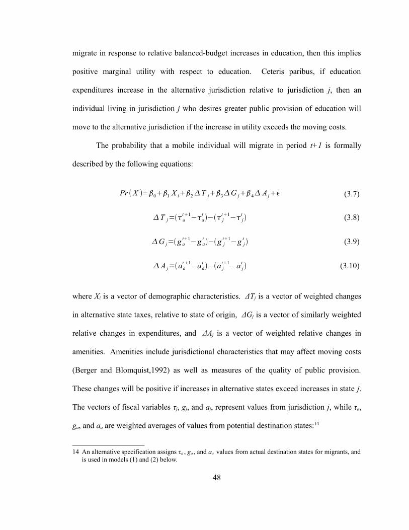
migrate in response to relative balanced-budget increases in education, then this implies
positive marginal utility with respect to education. Ceteris paribus, if education
expenditures increase in the alternative jurisdiction relative to jurisdiction j, then an
individual living in jurisdiction j who desires greater public provision of education will
move to the alternative jurisdiction if the increase in utility exceeds the moving costs.
The probability that a mobile individual will migrate in period t+1 is formally
described by the following equations:
Pr X =01 X i2T j3G j4 A j (3.7)
T j=at1−a
t − jt1− j
t (3.8)
G j=g at1−g a
t −g jt1−g j
t (3.9)
A j=aat1−aa
t −a jt1−a j
t (3.10)
where Xi is a vector of demographic characteristics. ΔTj is a vector of weighted changes
in alternative state taxes, relative to state of origin, ΔGj is a vector of similarly weighted
relative changes in expenditures, and ΔAj is a vector of weighted relative changes in
amenities. Amenities include jurisdictional characteristics that may affect moving costs
(Berger and Blomquist,1992) as well as measures of the quality of public provision.
These changes will be positive if increases in alternative states exceed increases in state j.
The vectors of fiscal variables τj, gj, and aj, represent values from jurisdiction j, while τa,
ga, and aa are weighted averages of values from potential destination states:14
14 An alternative specification assigns τa , ga , and aa
values from actual destination states for migrants, and is used in models (1) and (2) below.
48

gat = j
t (3.11)
at = j
t (3.12)
aat = j
t (3.13)
Γt, Θt, and Φt are matrices containing measures of expenditures, taxes, and amenities
respectively for each state at time t, and Ωj is a weighting matrix specific to jurisdiction j.
Five-year changes in the state of origin are compared to changes in alternative
states to create a measure of relative fiscal policy changes. Relative changes are the
change during the migration period in state levels of taxes and expenditures subtracted
from weighted nationwide average changes in state taxes and expenditures. Weighted
nationwide averages differ for each state, as alternative states weighted differently for
each state. The weighting matrix is similar to that used by Enchautegui (1997) and the
migration “flow” matrix used by Conway and Rork (2004). This weighting scheme uses
the actual number of migrants to destination states to create weights. Fiscal values for
alternative states are weighted by migrants to each alternative state as a fraction of total
outmigration from the home state j. Figure 3.1 illustrates this calculation. Potential
alternative states containing no immigrants originating from jurisdiction j are assigned a
weight of zero. Weighted values of each alternative state are summed to then generate τa ,
ga, and aa, which represent taxes, public provision, and amenities, respectively. This
“flow” method has the advantage of making no assumptions about determinants of
migration or moving costs, as it uses actual decisions made by individuals to predict
49

alternatives. For migrants, actual values for destination states are used in one
specification while predicted values are used in another specification.
Figure 3.1: Migration Weights
4 Out-Migrants 2 Out-Migrants
3 Out-Migrants
In this example, the tax increase in the theoretical next-best alternative state would be:
4⋅2%2⋅5%−3⋅3%423
= 2%
These specifications allow examination of fiscal changes in other states relative to
changes in the state of origin, and can be used to determine which changes are likely to
induce migration. These models are estimated using a logit procedure. Marginal effects
are calculated according to Anderson and Newell (2003).
Sonstelie and Portney (1978) suggest that municipalities can alter property values
with public provision and Brueckner (1982) describes a test that can be used to determine
provision levels that maximize property values. By constructing a relationship between
fiscal policy and the probability of attracting mobile individuals, this idea can be
50
AlternativeState A2% TaxIncrease
AlternativeState B5% TaxIncrease
Initial State
AlternativeState C3% Tax
Decrease

modified to create a test for optimal provision. In order to determine what fiscal policies
will maximize the probability that individuals will locate in a given jurisdiction, a
quadratic can be estimated.
Pr X =01T j2T j23G j4G j
2 (3.14)
12⋅2T j (3.15)
32⋅4G j (3.16)
Equation (3.14) will produce estimates of the effects on migration for a marginal
change in state characteristics. Equations (3.15) and (3.16) represent the marginal effect
of taxes and public provision, respectively. Figure 3.2 shows this relationship
graphically. P(Q) represents the probability that a mobile individual will reside in the
jurisdiction at the end of the migration period, either because they decided not to
emigrate, or they immigrated from another jurisdiction. Q represents balanced budget
public provision, since provision must be financed with taxes. Q represents g = τ for a
particular jurisdiction.
In reality, political rent and bureaucratic inefficiencies cause the total amount of τ
to exceed the value of g provided, and individuals will prefer a lower level of provision
than they would in a purely Pigouvian world with no inefficiencies. Q* represents the
optimal quantity of public provision when government inefficiencies are considered,
while QP represents that in a Pigouvian world. This study assumes that any inefficiencies
remain constant and similar across jurisdictions throughout the migration period, and
therefore have no bearing on individual migration decisions.
51

At extreme levels of Q, individuals will find the jurisdiction undesirable, either
due to low levels of provision or high taxes. Q* represents the level of Q that maximizes
the probability of attracting mobile residents. This also represents the optimal level of Q,
or “bliss point” according to mobile individuals. This relationship can be modeled with a
quadratic. At levels near Q*, marginal changes in Q will have little effect on P(Q). At
levels above (below) Q*, marginal increases will decrease (increase) P(Q). By observing
the changes in P(Q) associated with a given change in Q, we can observe the slope of
P(Q) for a particular value of Q. Using this information, Q* would be the level of Q for
which the slope would be zero for a marginal change in Q.
Figure 3.2: Migration and Public Provision
P(Q)
Q* QP Q
While Figure 3.2 represents the aggregation of the migration response curves for
all individuals in an economy, the relationship between P(Q) and Q is different for every
subgroup. Figure 3.3 shows this relationship for an economy with 2 subgroups. QH
52

represents the quantity of public provision that coincides with the bliss point for high-
income individuals, while QL represents the quantity that coincides with low-income
individuals. When individuals are aggregated, the economy-wide migration response
curve emerges. In general, fiscal policy may have a greater effect on the migration
decisions of high income individuals simply because they are more mobile to begin with.
If this is true, then the provision of QH will have a greater effect on the probability of
migration for high-income individuals than the provision of QL will have on low-income
individuals.
Figure 3.3: Disaggregated Migration and Public Provision
P(Q)
High Income Migrants
Low Income Migrants
QH Q* QL Q
If high-income individuals do prefer less public provision, then provision levels
below Q* will tend to attract a higher percentage of these individuals, ceteris paribus. In
certain cases this can change the demographic makeup of the population. At the most
extreme example with perfect mobility, provision levels would have a homogenizing
effect on the population (Tiebout, 1956). In the absence of perfect mobility, the
53
PH(QH)
PL(QH)

population may remain heterogeneous (Rhode and Strumpf, 2003). If QH is provided,
this will maximize the probability that mobile high-income individuals will locate in the
jurisdiction in question. This probability is represented by PH(QH). PL(QH) represents the
probability that a low-income individual will locate in the jurisdiction in question under
QH. Marginal increases from QH would be expected to increase the probability that low-
income individuals will locate in the jurisdiction. Through disaggregation, estimates will
produce preferred levels of provision for different subgroups.
In aggregate studies, the number of individuals that migrate to a certain state will
affect the fiscal policies of that state. If fiscal policy can attract migrants, but migrants
also affect fiscal policy, estimates will suffer from endogeneity bias. Because this study
uses micro data, endogeneity is assumed to not be present. Individuals do not take into
consideration the effect of their migration decision on the fiscal policies of their
destination state. Because migrants represent a minority of the overall population, it is
assumed that their decisions will have a relatively small effect on overall fiscal policies.
To the extent that policy change can be driven by mobile individuals, an aggregation
issue may still exist.
Data
As is common practice in migration studies, the analysis is restricted to the 48
contiguous U.S. States. State-level fiscal data from 1985-1990 and 1995-2000 are taken
from the Census Bureau. Measures of various taxes collected from own sources and
expenditures are converted to dollars per $1000 of personal income and dollars per
capita. These are then used to construct data on fiscal changes over the two migration
54
periods. Table 3.1 provides the average initial values of these fiscal measures for these
48 states.
These measures represent average levels of taxes and expenditures, and may not
represent actual levels experienced by a particular individual. While individual-level tax
estimates are available through NBER's Taxsim, it is more difficult to obtain accurate
individual-level estimates of burdens for other tax instruments. For this reason, estimates
of individual responses created from this data represent responses to average changes in
taxes rather than responses to changes in taxes for a particular subgroup.
Expenditures exceed state tax receipts since a large degree of expenditures are
financed with debt or federal funds. If the sum of changes in expenditures is equal to the
sum of changes in revenues, equations (3.7) and (3.14) will be unidentified. For this
reason, intergovernmental transfers are excluded as a source of revenue. Average 5 year
changes are provided in Table 3.2.
On average, real per capita total taxes rose by $511.59, from $1,768.73 to
$2,280.32, an increase of 29 percent. Similarly, expenditures rose by $995.05, from
$3,691.83 to $4,686.88, an increase of 27 percent. Relative changes are created from
these original fiscal changes by comparing the changes in the initial state to the changes
in the “next best” state. Fiscal policy changes in a theoretical “next-best” state are
computed using the weighting method discussed in the previous section. For migrants,
relative changes are constructed using two different methods. The first method, used by
Enchautegui (1997), compares changes in the initial state to changes in actual destination
states, while the second method assigns the same imputed values as with nonmigrants.
55

Individual-level data was taken from the decennial census. Demographic
information includes age, race, education, income, and number and age of children.
Table 3.3 provides summary demographic statistics by education and household income.
Data on migration is also taken from the decennial census, and results from
geographic location at the time of the census and a question asking individuals where
they lived 5 years ago. Those who lived in a different state are classified as migrants,
while those in the same state are considered non-migrants. Kaplan and Schulhofer-
Wohl (2010) find that in 2000, previous state locations were imputed by the Census
Bureau for individuals who did not respond to questions in the Current Population Survey
about migration. This process was more likely to assign alternative previous states to
those who did not migrate across state lines than to assign the same previous state to non-
respondents who actually did. Because of this, the data tends to overstate the number of
individuals who migrated. They find that from 1999-2005, the interstate migration rate
for the 10 to 12 percent of CPS respondents with imputed data is 3 to 5 times greater than
that of those with actual data. A lower 2 percent of the data in the 2000 decennial census
was imputed, and this bias will therefore be less prevalent in the decennial census (Nash,
2001). However, imputations that do exist in the decennial census could cause this study
to overstate the propensity of individuals to migrate in response to fiscal policy, as this
analysis relies heavily on migrant data.
Table 3.4 shows the average 5-year real changes experienced by individuals,
broken down by migrant status, education, and age. Ceteris paribus, younger individuals
and those with more years of education tend to be more likely to migrate. In all cases,
56

migrants experienced smaller increases in taxes and expenditures than nonmigrants.
While this is consistent with the idea that migrants are moving away from balanced
budget fiscal activity, this is also consistent with the idea that migrants are moving to
dense areas that experience economies of scale in public provision. Increases per capita
along with decreases as a share of personal income suggest that, for migrants, personal
income increased at a faster rate than taxes and expenditures.
In order to control for the quality of public provision, per capita violent crimes
data is taken from the Bureau of Justice Statistics. Average college entrance exam scores
by state are taken from ACT to be used as a proxy for school effectiveness. Average
energy costs by state are taken from the Energy Information Administration.
Results
Table 3.5 presents marginal effects for the logit models of equation (3.14) using
overall taxes and expenditures, per capital fiscal measures and the full sample. Models
(1) and (2) use imputed fiscal measures for alternative states for nonmigrants. Actual
alternative state values are used for migrants. Model (2) introduces quadratic terms for
taxes and expenditures. Models (3) and (4) are analogous, but use imputed values for
alternative states for all individuals. In general, taxes repel individuals and expenditures
attract individuals. For models (1) and (3), Wald tests reject the hypothesis that the net
effect of taxes and expenditures is zero with a confidence level in excess of 99%. As the
effects of taxes are larger in magnitude than the effects of expenditures, and the net effect
of additional fiscal activity is to reduce the probability that an individual will locate in a
particular jurisdiction. This suggests that mobile individuals are choosing to locate in
57

areas where fiscal government is growing at a slower rate. A $1000 per capita increase in
expenditures financed with state or local taxes would reduce the probability that an
individual will locate in the jurisdiction by 0.58 percent in model (1), and 2.29 percent in
model (3).
The quadratic specification in models (2) and (4) can be used to find estimates of
critical points for relative changes in taxes and expenditures. In model (2), the critical
point for tax changes is $0.65. In model (4), the critical tax change is -$1.70. The critical
expenditure change is $0.48 in model (2) and $1.30 in model (4). These estimates may
be of questionable use. Theoretically, all these critical points should represent maxima,
however, only relative taxes for model (4) represents a maxima. In the other cases the
estimated coefficients on the quadratic terms are positive, and the critical points derived
from these estimates represent minima. The models in these cases are fitting quadratics
that are convex with respect to the origin, suggesting that the data does not follow the
shape predicted in Figure 3.2. For the ranges of fiscal variables in the data, migration
responses could follow a shape similar to that of high income individuals at a high level
of public provision shown in Figure 3.3. In other words, over the range of fiscal changes
in the data, migration responses could be convex with respect to the origin because we
are in the tail of the normal distribution.
Another explanation is that groups may be polarized politically within
demographically homogeneous groups. There may be considerable divergence between
Democrats and Republicans, for example, within a relatively homogeneous community.
Some may care more about increasing expenditures while others may care more about
58

reducing taxes. This could generate a situation highlighted by Alesina, Baqir and
Easterly (1999), where the average individual's preference is, on average, considerably
different than that of the “median voter,” though policies are still dictated by the median
voter. In these cases, the data points may be following more extreme versions of the
subgroup migration response curves shown in Figure 3.3. This is illustrated below in
Figure 3.4. In this case, a median level of Q is set as a compromise between low levels of
provision and high levels of provision that would be preferred by one of the two
subgroups. This median level is not considered optimal by most individuals.
Consequently, marginal changes will attract one group but repel the other. A marginal
increase from Q* would repel some individuals who desire lower levels of provision, but
may attract substantially more individuals who desire higher levels of provision, and vice
versa. Q* may actually appear to minimize the probability that all individuals locate in
the jurisdiction. This probability, which is the sum of the probability curves for both
groups, is represented by the dotted line in Figure 3.4. If we never empirically observe
Q* falling below QL or above QH, then we might expect a quadratic model to fit a convex
curve. However, even when relatively small subsamples are considered in quadratic
models, minima persist.
59
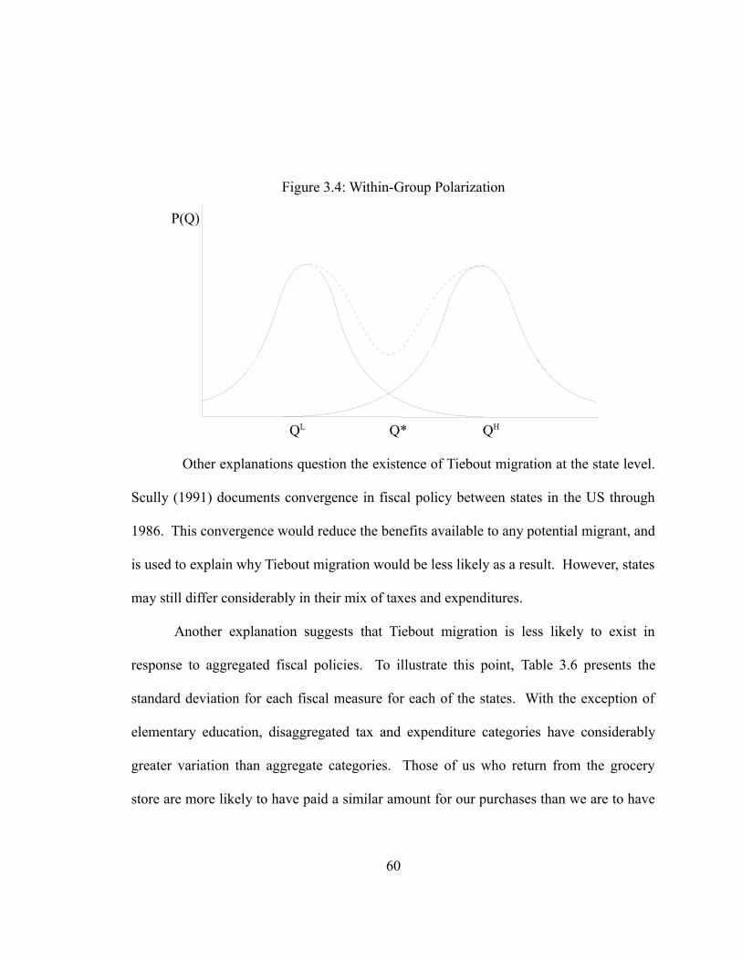
Figure 3.4: Within-Group Polarization
P(Q)
QL Q* QH
Other explanations question the existence of Tiebout migration at the state level.
Scully (1991) documents convergence in fiscal policy between states in the US through
1986. This convergence would reduce the benefits available to any potential migrant, and
is used to explain why Tiebout migration would be less likely as a result. However, states
may still differ considerably in their mix of taxes and expenditures.
Another explanation suggests that Tiebout migration is less likely to exist in
response to aggregated fiscal policies. To illustrate this point, Table 3.6 presents the
standard deviation for each fiscal measure for each of the states. With the exception of
elementary education, disaggregated tax and expenditure categories have considerably
greater variation than aggregate categories. Those of us who return from the grocery
store are more likely to have paid a similar amount for our purchases than we are to have
60

purchased a similar basket of goods. In the same way, individuals are more likely to
prefer different types of public provision than they are to prefer different expenditure
levels. Consequently, it may be more difficult to observe Tiebout-style migration in
response to aggregate expenditures than in response to individual expenditures.
Table 3.7 presents estimates using fiscal measures as a share of every $1000 in
personal income. Models (5) and (6) use actual values for migrants, while models (7)
and (8) impute values for migrants. The income share models differ from the per capita
models in that they suggest that individuals are migrating toward balanced budget
increases in provision. Model (5) suggests a $1 increase in expenditures financed
through additional taxes will increase the probability that an individual locates in the
jurisdiction by 0.097 percent, while model (7) suggests only 0.009 percent. Model (6)
fits a quadratic, and suggests critical relative decreases of $0.34 and $2.20 on taxes and
expenditures respectively. Model (8) also fits a quadratic, and suggests a decrease $6.00
for every $1000 of personal income in expenditures will maximize the probability of
location in a jurisdiction at the end of the migration period. Model (8) fits a convex
quadratic for taxes and suggests that a decrease of $6.25 will minimize the probability of
location in a jurisdiction. These quadratic estimates would also be subject to the caveats
discussed above.
The per capita measures are common in the literature, but can be criticized as the
cost of living varies across jurisdictions. Expenditures, while nominally greater in one
jurisdiction, may represent a lower level of public provision. Measures as a share of
personal income may overcome this limitation but may be subject to other weaknesses.
61

Because many of the goods in question are at least partially nonrival, relatively large
jurisdictions may realize significant economies of scale. If states with larger tax bases
can take advantage of economies of scale, expenditures as a share of personal income
may be lower than in a competing state even if the actual level of provision is higher.
A third specification uses per capita measures of expenditures in combination with
taxes as a share of personal income. The intuition is that individuals care about their tax
liabilities in proportion to their income, but do not consume publicly-provided goods in
proportion to their income. Estimates using this specification are also shown in Table
3.7. The marginal impact of balanced budget fiscal activity was calculated at the mean
income for all individuals. In a quasi-R2, the estimated coefficients from this model have
a predictive ability of somewhere between 2.59 and 6.33 percent greater than the constant
term alone (Shtatland et al,2000).
Table 3.8 provides results using data from the 1990 census for comparison. The
linear models produce evidence that individuals are moving away from taxes and towards
expenditures. On net, individuals are moving towards balanced budget increases in fiscal
activity. All four quadratic models in Table 3.8 fit convex functions, suggesting that the
critical tax increases and expenditure decreases appear to minimize the probability that
individuals will locate in a jurisdiction.
Table 3.9 reports income and tax coefficients for models (1) through (8) estimated
using a restricted sample that excludes individuals nearing retirement age. Results are
generally similar, with the exception of model (1) which suggests the relative balanced
62
budget increases in fiscal activity is positively associated with locational decisions. In
general, the imputed data provides smaller estimates of the effect of expenditures.
Table 3.10 presents the 2000 and 1990 results of linear models estimated with
disaggregated taxes and expenditures. Alternative state data is imputed for all individuals
in these models. These models allow the marginal effect of a balanced budget increase in
specific types of expenditures to be calculated. New expenditures are assumed to be
financed using different tax instruments in proportion to their original distribution as
shown in Table 3.1.
With the exception of corporate income taxes in the 1985-1990 migration period
and estate taxes for the 1995-2000 period, these models generate negative coefficients for
all taxes. Though the coefficient on estate taxes appears large, a $1 increase would more
than double estate taxes from the 1995 level of .73 for every $1,000 of personal income,
while a $1 increase in other taxes would be relatively small.
In general, education expenditures are positively related to migration decisions,
while expenditures in other categories are negatively related. This is consistent with the
conclusions of Evans and Karras (1994), who find that public expenditures on education
are productive and contribute to economic growth, but other expenditures do not. For the
1990 Census, welfare expenditures are positively related and higher education
expenditures are negatively related to migration decisions.
It seems counterintuitive that individuals would migrate away from increases in
safety, highway, and utility spending, given the theoretical idea and empirical
confirmation in Table 3.7 that individuals are attracted by public provision. This may be
63

attributable to characteristics of specific types of provision and unobservables. Spending
on public safety programs is valued in order to protect individuals from crime, a
characteristic that would tend to drive away mobile individuals, and for this reason
violent crime is included in the model as a control variable. Beyond crime control,
however, police and corrections services are of questionable value. Individuals may be
migrating away from areas with relatively large public safety programs but relatively
little crime. Additional expenditures in this case would be relatively ineffective,
compared to areas with high crime and low police expenditures.
Ceteris paribus, individuals should prefer additional spending on highways,
though individuals appear to migrate away from it. If spending on roads follows
disrepair, traffic congestion and need for new construction, a measure of this type of
spending may be a proxy for poor transportation infrastructure.
Certain types of provision, such as public utilities are commonly privatized. In
these cases, public spending on these programs will fall dramatically, though the
programs themselves remain in place. If inefficiencies provided incentives for
privatization, which in fact resulted in more efficient provision, then the public would be
more satisfied with the program, even though public spending on the program fell. This
may also be the case with highways, as toll roads in some states are privatized.
Table 3.11 presents the marginal effect of balanced budget changes for a variety of
demographic subsamples. Results are provided for subsamples in order to examine the
interaction effects of income, age and education. These subsamples demonstrate
considerable heterogeneity in willingness to pay for public provision. Most surprising is
64

the negative sign on balanced budget increases in welfare expenditures for low income
individuals. Results are similar for single-female-headed households at the bottom
quintile of the income distribution, a group that has traditionally had a strong empirical
link with welfare migration. These results require explanation.
When taxes are not considered, the marginal effect of relative changes in welfare
expenditures is positive for these individuals. This suggests that these balanced-budget
effects are being driven by individual responses to taxes. Low-income individuals have
different tax burdens than high-income individuals and are likely to pay the majority of
their taxes through different instruments. Low-income individuals, for example, are
likely to pay less through property and individual income taxes than are high-income
individuals. In addition, they are not likely to bear the full burden of additional welfare
expenditures with additional taxes. Therefore, these balanced-budget results should be
interpreted as the average individual's willingness-to-pay for additional quantities of
public provision, and do not conflict with previous empirical studies that document
welfare migration. Low-income individuals may not be “willing to pay” for additional
quantities of welfare expenditures, though they may still desire additional quantities and
may even be willing to engage in welfare migration, as evidenced by the positive
coefficients on welfare expenditures. In both cases, results indicate a negative
willingness-to-pay for all types of public provision.
Another puzzling result is the positive sign on balanced budget expenditures on
welfare and migration for the top income quintile. As would be expected, there is a
negative relationship between migration outcomes and welfare expenditures for this
65

group when taxes are not considered. Therefore, this result is driven solely by positive
coefficients on some of the tax variables. Only selective sales and corporate income
taxes generate negative coefficients for this group. As this group is more likely to receive
income from investments, they may prefer certain forms of taxes because the burden is
primarily borne by others. The relatively large coefficients on sales taxes may be positive
because sales taxes are thought to be more regressive, and these taxes are less likely to be
borne primarily by high-income individuals. Another explanation is that these tax
measures may be correlated with expenditure categories that high-income individuals
have strong preferences for. For example, relative changes in property taxes as a share of
personal income have a correlation with relative changes in expenditures on elementary
education of 0.36. Relative changes in individual income taxes have a correlation with
expenditures on higher education of 0.31. High income individuals may in fact dislike
taxes, but may value expenditures on education more. If this is the case, the coefficients
on property and income taxes will be upwardly biased, while the coefficients on
education will be downwardly biased. However, these two biases will tend to cancel
each other out when balanced budget changes are considered. These two examples
highlight the problem of examining individual group responses to aggregate tax changes.
Single-female-headed households in the bottom 20% if the income distribution do
not appear to be unsatisfied with the level of spending on safety programs including
police, fire, and corrections. These results differ from those of the full sample, which
migrate away from these expenditures. Perhaps these individuals are more likely to use
these services as they are more likely to live in low-income neighborhoods that are
66

inherently more dangerous. On the other hand, income constraints make these
individuals less likely to migrate, and they may be unable to escape from states with
increasing crime rates and increasing expenditures on these programs.
Policy makers may be most interested in attracting young college-educated
individuals. Estimates suggest that balanced-budget expenditures on elementary and
secondary education have the strongest positive relationship with migration for this
group. Expenditures on health programs have a smaller positive relationship, while other
expenditures have a negative relationship.
The final four columns in Table 3.11 provide estimates of the elasticity of
migration with respect to increases in fiscal categories broken down by educational
attainment. Individuals without a high-school diploma are less likely to migrate in
response to increases in expenditures on higher education. Similarly, individuals with a
high-school diploma but no college are likely to migrate away from increases in all fiscal
categories. Both of these results may partially be driven by the fact that these individuals
are unlikely to bear the full burden of any increases in taxes, and should be interpreted as
their willingness-to-pay for public provision, rather than their political preferences for
public provision. Those with some, but less than 4 years of college are migrating toward
balanced-budget increases in education expenditures. Interestingly, those with college
degrees seem willing to pay for increases in multiple types of expenditures, including
education, safety, and health.
Because different groups have different responses to changes in fiscal policies,
any changes to fiscal policy will have distributional implications. With the exception of
67

spending on higher education, fiscal policy changes are unlikely to attract one group
while repelling another. In most cases, all individuals would be attracted (or repelled) by
the same fiscal changes, but at different rates. These fiscal changes can have a larger
effect on individuals from a particular group.
Table 3.15 simulates the impact on the population of the average state of a $1
increase in each expenditure category financed with taxes. The data used to produce
these estimates is from a 1 in 20 sample of the underlying population, and results were
multiplied by 20 to produce simulated impacts on the underlying population. These
estimates use the mixed specification, and assume that individuals with larger incomes
will bear a larger share of the tax burden. Simulated impacts are calculated for various
demographic subcategories, including education, age, and income. In most cases,
education expenditures have a positive 5-year impact on population, while expenditures
in other categories tend to have a negative impact on population. Expenditures on higher
education tend to have a negative impact on the population with a high school diploma or
less education, as well as a negative impact on the population in the lower half of the
income distribution. These same expenditures on higher education tend to have a
positive impact on young individuals, those in the top half of the income distribution and
those with some college experience.
Higher education expenditures may in some cases attract those who wish to raise
their relatively low levels of education. Individuals respond to the Census survey with
their income and education levels at the end of the migration period, and some will have
had lower levels of income and education at the beginning of the migration period. In
68

some cases, individuals will have been attracted by states with higher education
expenditures that provide greater opportunities for individuals wishing to increase their
level of education.
Given that there are 171,421,060 individuals from the 48 continental states
represented in this study, there are approximately 3,571,272 individuals in the average
state. A $1 relative increase in expenditures per capita would therefore equate to an
annual increase of $3,571,272 in fiscal activity. Estimates of migration responses for
various demographic subgroups are presented in Table 3.12. These estimates are
produced using the number of individuals who actually moved during the migration
period as a base. A $1 increase in higher education expenditures per capita would attract
approximately 98 individuals to the average state over 5 years. In this case, the annual
cost to attract one of these individuals with higher education expenditures would be
approximately $36,441.55.
On the other hand, a $1 relative decrease (i.e., an annual reduction in fiscal
activity of $3,571,272) in expenditures per capita on police, fire, and corrections would
attract approximately 193 individuals in over years. In this case, approximately one
individual would be attracted for each $18,504.00 annual reduction in expenditures.
While this policy may increase the overall population, it may not be desirable as it also
slightly decreases the population of college-educated individuals and those in the top
income decile. Reductions in other programs, such as welfare and utilities, seem to
attract all individuals, but require larger annual reductions of $62,653.89 and $21,007.48
respectively, to attract one individual.
69

The estimates in Table 3.12 represent the average state, though there can be
considerable variation among states. For example, between 1995 and 2000, Florida was
more likely to attract individuals of retirement age, while Nevada was more likely to
attract young, single, college educated individuals. It is interesting to note that
individuals of retirement age do not appear to be affected by fiscal characteristics, though
a relatively large number are migrating to Florida. Many of these retired individuals are
likely migrating in search of unique amenities, and fiscal characteristics have relatively
little impact on their choices.
Tables 3.13, 3.14, and 3.15 provide estimates for Florida, Nevada, and Kentucky
respectively. Simulation estimates suggest that individuals can be attracted to Florida
with annual increases in higher education expenditures of $27,556.77, while Nevada can
attract individuals for $15,258.19. Because individuals are more likely to travel to these
states, marginal individuals can be attracted by these states with relatively low levels of
fiscal policy changes. On the other hand, individuals are less likely to travel to other
states. For example, Kentucky would have to spend approximately $40,229.06 in higher
education expenditures in order to attract or retain a mobile individual.
If individuals can be attracted with fiscal policy, then fiscal policy can also affect
the tax base in a jurisdiction. According to the Tax Foundation, the average state resident
in Florida, Nevada, and Kentucky paid $1,846, $1,423, and $1,183 respectively in state
taxes in 2000. While migrants are more likely to be high-income individuals who pay
higher than average taxes, it seems unlikely that tax receipts from these individuals would
be large enough to offset the cost to attract any of them with fiscal policy.
70

Conclusion
This chapter uses migration decisions to create revealed preference estimates of
willingness to pay for public provision. In general, high-income individuals and those
with a college education are more likely to be willing to pay for public provision.
Specifically, these individuals appear to be willing to pay for increases in expenditures on
education, and perhaps to a lesser extent, expenditures on healthcare. Most individuals
appear to be satisfied with the current level of spending on utilities, though those with a
college education seem to migrate away from it. This may be because they are migrating
into areas that are privatizing these functions. No one appears to be willing to pay for the
provision of highways. Expenditures on highways appear to have a positive benefit only
to low income individuals with less than a high school education. Perhaps high-income
individuals are migrating to areas with developed transportation infrastructures. These
areas may benefit from economies of scale and may be less likely to report an increase in
their per capita expenditures on roads.
Individuals are attracted to decreases in welfare spending. This also includes low-
income individuals who are more likely to benefit from such programs. While this may
seem counterintuitive, this result does not necessarily suggest that all low-income
individuals demand reductions in these programs, since there may be some unobservable
difference between low-income individuals who migrate and low-income individuals who
do not. However, this does suggest that welfare migration is not a significant problem,
and should not be used as a justification to reduce welfare spending and engage in a race-
to-the-bottom with other states.
71

According to these results, states that wish to attract (or create) young, relatively
high income, college educated individuals should increase spending on higher education
or health programs and finance this spending with reductions in spending on other
programs.
The ability of fiscal policy to homogenize a jurisdiction appears to be limited by
preexisting heterogeneity within the overall population. Young, educated and high
income individuals display higher intensity of preference. However, expenditures that
attract individuals from one group will likely attract individuals from other groups as
well. More radical changes in fiscal policies and/or other forms of government
intervention in the economy would likely produce more sorting and homogenization.
72

Table 3.1: Average Level of Taxes and Expenditure in 1995 (in 2000 Dollars)Per Capita Per $1000 of
Personal IncomeLevel Percentage Level Percentage
Total Taxes $1,768.73 - $69.96 -Property Taxes $614.54 34.74% $23.70 33.88%
General Sales Taxes $394.12 22.28% $16.01 22.89%Selective Sales Taxes $239.80 13.56% $9.52 13.61%
Individual Income Taxes $266.50 15.07% $10.50 15.02%Corporate Income Taxes $93.73 5.30% $3.67 5.25%
Estate Taxes $4.96 0.28% $0.18 0.26%Other Taxes $155.08 8.77% $6.37 9.10%
Total Expenditures $3,691.83 - $146.29 -Elementary Education $706.28 19.13% $28.32 19.36%
Higher Education $277.88 7.53% $11.29 7.72%Police, Fire, and
Corrections $182.75 4.95% $7.02 4.80%
Health and Hospitals $309.81 8.39% $12.47 8.52%Highways and Transportation $240.01 6.50% $9.63 6.58%
Welfare $565.34 15.31% $22.26 15.21%Utilities $234.16 6.34% $9.31 6.36%
Interest on Debt $211.08 5.72% $8.31 5.68%Other Expenditures15 $964.52 26.13% $37.68 25.76%
15 Includes all other expenditures. Values for this category are calculated by subtracting all other categories from total expenditures.
73

Table 3.2: Average 5-Year Change (2000 Dollars)Per Capita Per $1000 of
Personal IncomeTotal Taxes $511.59 $20.19
Property Taxes $92.62 $3.69General Sales Taxes $135.61 $5.42Selective Sales Taxes $41.97 $1.73
Individual Income Taxes $193.31 $7.50Corporate Income Taxes $3.04 $0.11
Estate Taxes $11.35 $0.44Other Taxes $33.69 $1.30
Total Expenditures $995.05 $40.52Elementary Education $245.63 $9.69
Higher Education $106.11 $4.36Police, Fire, and
Corrections $106.88 $4.34
Health and Hospitals $42.59 $1.84Highways and Transportation $85.83 $3.60
Welfare $97.45 $4.13Utilities $38.00 $1.50
Interest on Debt $17.40 $0.67Other Expenditures $255.17 $10.38
74

Table 3.3: Demographics and Migrants by Group, 2000 CensusEducation Full Sample Less than HS High School Some College College
N 8,571,053 1,671,182 2,579,283 2,341,035 1,979,553
Migrants 0.074 0.047 0.053 0.078 0.118
Household Income $63,494 $39,120 $51,640 $64,187 $98,699
Never Married 0.13 0.13 0.12 0.13 0.16
Female 0.53 0.52 0.54 0.55 0.50
Black 0.10 0.14 0.10 0.10 0.06
Hispanic 0.09 0.22 0.07 0.07 0.04
Avg Number of Children 0.65 0.61 0.61 0.73 0.69
Children (<6 yrs) Present 0.14 0.12 0.12 0.16 0.17
Older Children Present 0.28 0.25 0.27 0.31 0.28
Income Quantiles Bottom Income Quartile
25%-50% Income Quartile
50%-75% Income Quartile
Top IncomeQuartile
Top 5% Income Quantile
Top 1% Income Quantile
N 2,146,114 2,142,355 2,139,874 2,142,710 428,550 87,116
Migrants 0.065 0.073 0.074 0.084 0.093 0.092
Household Income $15,464 $37,810 $62,018 $138,760 $269,346 $432,130
Never Married 0.17 0.14 0.12 0.11 0.09 0.08
Female 0.60 0.52 0.50 0.50 0.49 0.49
Black 0.15 0.10 0.08 0.06 0.04 0.04
Hispanic 0.11 0.10 0.08 0.06 0.05 0.05
Avg Number of Children 0.51 0.67 0.76 0.71 0.70 0.81
Children (<6 yrs) Present 0.11 0.15 0.16 0.14 0.14 0.16
Older Children Present 0.21 0.27 0.32 0.32 0.30 0.34
75

Table 3.4: Average 5-Year Tax and Expenditure Changes by Group (Real 2000 Dollars)
Education Age N Migrants Fraction of Migrants
Real Tax Increase Experienced by
Migrants
Real Expenditure Increase Experienced
by Migrants
Real Tax Increase Experienced byNon-migrants
Real Expenditure Increase Experienced
by Non-migrants
Per Capita
Per $1000
Per Capita Per $1000
Per Capita Per $1000
Per Capita Per $1000
<HS
25-34 261,788 21,758 0.08 214.08 -0.44 943.68 19.25 422.09 2.74 1301.14 23.53
35-49 431,360 23,856 0.06 186.69 -1.11 924.63 19.25 404.50 2.30 1291.59 23.68
50-64 384,817 14,736 0.04 88.63 -2.72 828.10 19.42 376.05 1.57 1279.07 24.00
65+ 593,217 17,465 0.04 131.62 -3.05 874.11 17.37 361.53 1.08 1272.31 23.89
Total 1,671,182 77,815 0.05 163.42 -1.66 900.34 18.86 385.02 1.76 1283.15 23.81
HS
25-34 469,821 39,877 0.08 253.71 -0.41 1061.39 20.79 369.55 1.27 1277.26 23.79
35-49 908,028 48,764 0.05 207.84 -1.04 1005.97 20.81 359.69 0.91 1275.18 23.73
50-64 642,446 27,983 0.04 75.64 -3.18 822.90 19.09 354.22 0.72 1274.02 23.73
65+ 558,988 20,442 0.04 95.25 -3.81 826.85 16.47 357.34 0.59 1267.68 22.89
Total 2,579,283 137,066 0.05 177.40 -1.71 958.00 19.81 359.53 0.85 1273.60 23.56
HS+
25-34 531,414 63,368 0.12 285.41 -0.42 1112.41 20.30 388.30 1.61 1293.04 23.52
35-49 946,602 69,979 0.07 243.57 -0.68 1049.15 20.42 388.52 1.51 1290.79 23.19
50-64 551,836 34,765 0.06 136.83 -1.72 915.32 20.87 389.49 1.62 1289.76 23.30
65+ 311,183 15,444 0.05 102.35 -3.04 841.61 17.96 388.17 1.62 1281.22 23.08
Total 2,341,035 183,556 0.08 225.91 -0.99 1028.18 20.26 388.66 1.57 1289.72 23.27
College
25-34 443,495 100,831 0.23 377.12 -0.51 1258.96 18.95 394.54 1.34 1283.08 22.02
35-49 778,229 82,694 0.11 294.31 -0.90 1112.23 18.76 396.32 1.35 1276.83 21.73
50-64 503,452 36,115 0.07 163.68 -1.90 970.03 20.38 396.97 1.43 1279.20 21.92
65+ 254,377 14,445 0.06 64.21 -4.26 805.15 16.55 391.69 1.46 1274.31 22.20
Total 1,979,549 234,085 0.12 295.63 -1.09 1134.54 18.95 395.51 1.39 1278.34 21.90
Totals 8,571,053 632,522 0.07 233.51 -1.27 1036.61 19.51 380.47 1.35 1280.94 23.17
76

Table 3.5: Logit Estimation, Probability of Migration, Per Capita Fiscal Measures
Variable(1) (2) (3) (4)Non-Imputed Migrant Data Imputed Migrant Data
total taxes -0.000025 (0.000003)***
0.000065 (0.000002)***
-0.000003(0.000003)
-0.000017 (0.000003)***
total taxes2 0.000002 (0.000000)***
-0.0000002 (0.0000000)***
total expenditures 0.000043 (0.000001)***
0.000019 (0.000001)***
0.00001 (0.000001)***
-0.000013 (0.000002)***
total expenditures2 0.0000008 (0.0000000)***
0.0000002 (0.0000000)***
age -0.022357 (0.000145)***
-0.019048 (0.000048)***
-0.02246 (0.000147)***
-0.022529 (0.000145)***
age2 0.000145 (0.000001)***
0.000124 (0.000000)***
0.000146 (0.000001)***
0.000146 (0.000001)***
female -0.000839(0.000667)
0.000405(0.000594)
-0.000847(0.000666)
-0.000948(0.000667)
hispanic -0.029108 (0.001311)***
-0.04419 (0.001168)***
-0.037706 (0.001315)***
-0.038418 (0.001315)***
black -0.049961 (0.001226)***
-0.007126 (0.00108)***
-0.053417 (0.001227)***
-0.053389 (0.00123)***
highschool 0.000634(0.001189)
0.003947 (0.001052)***
0.002098 (0.001188)*
0.002304 (0.001188)*
somecollege 0.086423 (0.001149)***
0.06586 (0.001165)***
0.08601 (0.001146)***
0.085761 (0.001149)***
college 0.199108 (0.001128)***
0.161148 (0.001522)***
0.198909 (0.001125)***
0.198413 (0.001129)***
single -0.02041 (0.001003)***
-0.025278 (0.000852)***
-0.02044 (0.001004)***
-0.021157 (0.001003)***
child < 6 -0.00349 (0.00124)***
-0.002434 (0.0011)**
-0.004201 (0.001239)***
-0.00445 (0.00124)***
child > 5 -0.078228 (0.00131)***
-0.067246 (0.001241)***
-0.078612 (0.001309)***
-0.07872 (0.00131)***
number of children 0.005701 (0.000636)***
0.00505 (0.000567)***
0.006028 (0.000636)***
0.00617 (0.000636)***
unemployment -0.03117 (0.000674)***
-0.066637 (0.000763)***
-0.019398 (0.000706)***
-0.011568 (0.000773)***
poverty 0.001236 (0.00018)***
0.000002(0.00017)
0.003263 (0.000186)***
0.005166 (0.00019)***
energy prices 0.019845 (0.000953)***
-0.0186 (0.000927)***
0.027814 (0.000996)***
0.038261 (0.001039)***
test scores 0.012907 (0.001289)***
-0.000765(0.001198)
0.045585 (0.001365)***
0.041223 (0.001366)***
violent crime -0.008492 (0.000418)***
-0.011206 (0.000383)***
-0.002827 (0.000442)***
-0.005612 (0.000445)***
population density -3.53e10 (1.76e10)**
-1.26e12 (1.73e10)***
9.85e10 (1.83e10)***
-5.43e11 (2.16e10)***
* , **, and *** indicate p<0.10, p<0.05, and p<0.01, respectively.
77

Table 3.6: Relative Standard Deviation, Fiscal Measures
Tax Category Relative Standard Deviation Expenditure Category Relative Standard
Deviation
Per Capita Per Income Per Capita Per Income
Property Taxes 52.20 47.64 Elementary Education 30.08 27.55
General Sales Taxes 52.66 52.98 Higher Education 40.61 45.75
Selective Sales Taxes 67.92 68.24 Police, Fire, and Corrections 36.93 36.91
Individual Income Taxes 72.21 62.98 Health and Hospitals 104.30 101.82
Corporate Income Taxes 301.55 276.42 Highways and Transportation 71.15 69.33
Estate Taxes 122.94 124.96 Welfare 72.75 77.56
Other Taxes 311.83 287.55 Utilities 105.94 97.78
Other Expenditures 58.35 55.08
Total Taxes 39.91 34.17 Total Expenditures 25.54 28.79
78

Table 3.7: Logit Estimation, Probability of Migration, Per Capita, Per Income, and Mixed Fiscal Measures
2000 Census
(1) (2) (3) (4) (5) (6) (7) (8) (9) (10) (11) (12)
Per CapitaRelative Changes in Per Capita Tax and Expenditure Categories
Per IncomeRelative Changes in Tax and Expenditure Categories for
each $1000 of Personal Income
Mixed Relative Changes in Tax Categories as a Share of Mean Personal Income Combined with Relative Changes in
Expenditure Categories Per CapitaNon-Imputed Migrant Data Imputed Migrant Data Non-Imputed Migrant Data Imputed Migrant Data Non-Imputed Migrant Data Imputed Migrant Data
total taxes -0.000025 (0.00000)***
0.000065(0.00000)***
-0.00003 (0.00000)***
-0.000017(0.00000)***
-0.0003 (0.0001)***
0.0017 (0.0001)***
-0.00009 (0.00008)
-0.0005 (0.0001)***
-0.0001 (0.0001)
-0.0043 (0.0001)***
0.00039(0.00008)
0.00004(0.00009)
total taxes2 0.000002(0.00000)***
-0.0000002(0.00000)***
0.0022 (0.0000)***
-0.00007 (0.00000)***
-0.0021 (0.00001)***
-0.00012 (0.00000)***
total expenditures
0.000043 (0.00000)***
0.000019(0.00000)***
0.00001 (0.00000)***
-0.000013(0.00000)***
0.0010 (0.0000)***
0.0022 (0.0000)***
0.0004 (0.0000)***
0.0006 (0.0000)***
0.00004 (0.00000)***
0.00004 (0.00000)***
0.0000059(0.0000017)
0.00001 0.00000)***
total expenditures2
0.0000008(0.00000)***
0.0000002(0.00000)***
0.0005 (0.0000)***
0.00005 (0.00000)***
8.64e-7(5.63e-9)***
-1.7e-7(3.37e-9)**
net impact, additional $1
fisc0.002% -0.002% 0.07% 0.031% 0.03% 0.04%
critical tax change $0.65 -$1.70 -$0.32 -$0.28 -$1.02 $0.17
critical expenditure
change$0.48 $1.30 -$2.20 -$0.17 -$23.15 $29.41
Table 3.8: Logit Estimation, Probability of Migration, Per Capita and Per Income Fiscal Measures, 1990 1990 CensusN=7,628,856
(Imputed Migrant Data)
(3) (4) (5) (6)
Per CapitaRelative Changes in Per Capita Tax and Expenditure Categories
Per IncomeRelative Changes in Tax and Expenditure Categories for each $1000 of
Personal Income
total taxes -0.00004 (0.00000)***
-0.00015 (0.00000)***
-0.00003 (0.00000)***
-0.00198 (0.00088)***
total taxes2 0.0000002 (0.0000000)***
0.000031 (0.000001)***
total expenditures 0.00001 (0.00000)***
0.00007 (0.00000)***
0.00001 (0.00000)***
0.00073 (0.00004)***
total expenditures2 0.00000015 (0.00000000)***
0.00006 (0.00001)***
net impact, additional $1 fisc 0.005% 0.10%critical tax change $460.80 $32.38
critical expenditure change -$234.15 -$5.98
79
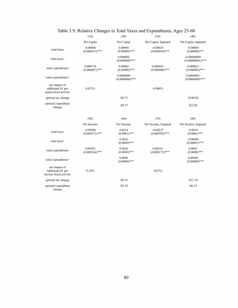
Table 3.9: Relative Changes in Total Taxes and Expenditures, Ages 25-60(1b) (2b) (3b) (4b)
Per Capita Per Capita Per Capita, Imputed Per Capita, Imputed
total taxes -0.00006 (0.000015)***
0.00004 (0.00000)***
-0.00010 (0.000016)***
-0.00004 (0.00000)***
total taxes2 0.000002 (0.000000)***
-0.00000009 (0.00000001)***
total expenditures 0.000170 (0.000007)***
0.00002 (0.00000)***
0.000041 (0.000008)***
-0.000011 (0.000002)***
total expenditures2 0.0000009 (0.0000000)***
0.0000002 (0.0000000)***
net impact of additional $1 per
capita fiscal activity0.011% -0.006%
optimal tax change -$8.71 -$189.96
optimal expenditure change -$9.57 $32.08
(5b) (6b) (7b) (8b)
Per Income Per Income Per Income, Imputed Per Income, Imputed
total taxes -0.00286 (0.000371)***
0.0018 (0.0001)***
-0.00237 (0.000392)***
-0.0010 (0.0001)***
total taxes2 0.0026 (0.0000)***
-0.00004 (0.00001)***
total expenditures 0.00383 (0.000166)***
0.0026 (0.0000)***
0.00163 (0.000175)***
0.0005 (0.0000)***
total expenditures2 0.0006 (0.0000)***
0.00004 (0.00000)***
net impact of additional $1 per
income fiscal activity0.10% -0.07%
optimal tax change -$0.35 -$11.78
optimal expenditure change
-$2.19 -$6.15
80

Table 3.10: Full Sample, 2000 and 1990 Censuses2000 Census (N=8,571,053) 1990 Census (N=7,628,856)
Variable Per Capita Per Income Mixed Per Capita Per Income
Δ Property Tax -0.0002 (0.0000)***
-0.0036 (0.0003)***
-0.0044 (0.0003)***
-0.00004 (0.00001)***
-0.0010 (0.0001)***
Δ General Sales Tax -0.00005 (0.00001)***
-0.0008 (0.0002)***
0.0007 (0.0002)***
-0.00004 (0.00001)***
-0.0003 (0.0001)**
Δ Selective Sales Tax -0.0004 (0.0000)***
-0.0087 (0.0003)***
-0.0078 (0.0003)***
-0.0007 (0.0000)***
-0.0104 (0.0003)***
Δ Individual Income Tax -0.00014 (0.00001)***
-0.0026 (0.0001)***
-0.0024 (0.0001)***
-0.0002 (0.0000)***
-0.0032 (0.0001)***
Δ Corporate Tax -0.0004 (0.0000)***
-0.0099 (0.0006)***
-0.0047 (0.0006)***
0.00013 (0.00003)***
0.0060 (0.0005)***
Δ Estate Tax 0.00022 (0.00006)***
0.0080 (0.0015)***
0.0064 (0.0015)***
-0.0011 (0.0001)***
-0.0153 (0.0017)***
Δ Interest on Debt -0.000022(0.000018)
-0.0016 (0.0005)***
0.0008(0.0005)
-0.0008 (0.0000)***
-0.0137 (0.0003)***
Δ Elementary Education 0.0003 (0.0000)***
0.0064 (0.0001)***
0.0002 (0.0000)***
0.0005 (0.0000)***
0.0082 (0.0001)***
Δ Higher Education 0.0003 (0.0000)***
0.0072 (0.0003)***
0.0003 (0.0000)***
-0.00011 (0.00002)***
-0.0021 (0.0003)***
Δ Safety -0.0003 (0.0000)***
-0.0078 (0.0004)***
-0.0003 (0.0000)***
-0.0005 (0.0000)***
-0.0101 (0.0004)***
Δ Health and Hospitals -0.00011 (0.00001)***
-0.0017 (0.0002)***
-0.00008 (0.00001)***
-0.00014 (0.00001)***
-0.0019 (0.0002)***
Δ Highways -0.00010 (0.00001)***
-0.0032 (0.0003)***
-0.00008 (0.00001)***
-0.00008 (0.00001)***
-0.0009 (0.0002)***
Δ Welfare -0.000004(0.000006)
-0.0007 (0.0001)***
-0.00003 (0.00001)***
0.0002 (0.0000)***
0.0034 (0.0002)***
Δ Utilities -0.0003 (0.0000)***
-0.0054 (0.0003)***
-0.0003 (0.0000)***
0.00012 (0.00001)***
0.0014 (0.0001)***
Δ Other Taxes -0.00011 (0.00001)***
-0.0039 (0.0004)***
-0.0037 (0.0004)***
0.0004 (0.0000)***
0.0047 (0.0002)***
Δ Other Expenditures 0.00009 (0.00001)***
0.0024 (0.0001)***
0.00006 (0.00001)***
0.00010 (0.00001)***
0.0021 (0.0001)***
Effect of Balanced Budget Changes on P(x)Elementary Education 0.0116*** 0.2804*** 0.0154*** 0.0356*** 0.6413***Higher Education 0.0105*** 0.3564*** 0.0229*** -0.0231 -0.3841Safety -0.0461*** -1.1431*** -0.0418*** -0.0659*** -1.1847***Health and Hospitals -0.0287*** -0.5308*** -0.0166*** -0.0262 -0.3657Highways -0.0275*** -0.6778 -0.0173*** -0.0204** -0.2633***Welfare -0.0180*** -0.4257*** -0.0114*** 0.0032 0.1678***Utilities -0.0432*** -0.8958*** -0.0367*** -0.0004*** -0.0329***Other Expenditures -0.0088*** -0.1228*** -0.0026*** -0.0019*** 0.0298***
81
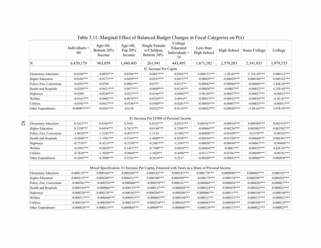
Table 3.11: Marginal Effect of Balanced Budget Changes in Fiscal Categories on P(x)
Individuals < 60
Age<60, Bottom 20%
Income
Age<60, Top 20% Income
Single Female w/Children,
Bottom 20%
College Educated
Individuals < 35
Less than High School High School Some College College
N 6,420,179 963,059 1,440,403 261,941 443,495 1,671,182 2,579,283 2,341,035 1,979,553$1 Increase Per Capita
Elementary Education 0.0109*** -0.0055*** 0.0304*** -0.0057*** 0.0385*** 0.000171*** -1.2E-05*** 5.31E-05*** 0.000113***Higher Education 0.0106*** -0.0171*** 0.0459*** -0.0187*** 0.0472*** -0.00029*** -0.00029*** 0.000188*** 0.000192***Police, Fire, Corrections -0.0391*** -0.0704 0.0001*** -0.0757 0.0127** -0.00043*** -0.00084*** -0.00068*** 1.44E-05***Health and Hospitals -0.0289*** -0.0621*** 0.0077*** -0.0690*** 0.0116*** -0.00038*** -0.0007*** -0.00032*** 6.35E-05***Highways -0.0309 -0.0249*** -0.0237*** -0.0166*** -0.0446*** -5.9E-05*** -0.00027*** -0.00027*** -0.00013***Welfare -0.0161*** -0.0402*** 0.0074*** -0.0354*** -0.0016** -0.00023*** -0.00032*** -0.00018*** -6.3E-07***Utilities -0.0383*** -0.0637*** -0.0146*** -0.0580*** -0.0281*** -0.00054*** -0.00067*** -0.00035*** -0.00011***Other Expenditures -0.000071*** -0.0301*** 0.0150 -0.0222*** 0.0116*** -0.00022*** -0.00024*** -5.5E-05*** 3.07E-05***
$1 Increase Per $1000 of Personal IncomeElementary Education 0.2412*** 0.0346*** 0.5942 0.0325*** 0.8253*** 0.005567*** -0.00016*** 0.000589*** 0.002519***Higher Education 0.3338*** 0.0454*** 0.7623*** -0.0146*** 0.7509*** -0.00444*** -0.00236*** 0.005885*** 0.003582***Police, Fire, Corrections -1.0034*** -1.2243*** -0.4937*** -1.3134 -0.1802*** -0.00808*** -0.01859*** -0.0176*** -0.00102***Health and Hospitals -0.5698*** -1.3501*** 0.3336*** -1.4409*** 0.4538*** -0.00636*** -0.01558*** -0.00664*** 0.002391***Highways -0.7710** -0.4215*** -0.7539*** -0.2461*** -1.3591*** -0.00058*** -0.00499*** -0.00667*** -0.00408***Welfare -0.3991*** -0.8824*** 0.1421*** -0.7308*** -0.0818*** -0.00464*** -0.0081*** -0.00475*** 4.43E-05***Utilities -0.7828*** -1.5920*** -0.0604*** -1.3628** -0.4496*** -0.01117*** -0.01561*** -0.00699*** -0.00181***Other Expenditures -0.1042*** -0.5088*** 0.3536*** -0.2814*** 0.2517 -0.00289*** -0.00433*** -0.00068*** 0.000839***
Mixed Specification: $1 Increase Per Capita, Financed with Taxes as a Share of Personal IncomeElementary Education 0.000135*** 0.000166*** 0.000240*** 0.000162*** 0.000347*** 0.000179*** 0.0000003*** 0.000062*** 0.000105***Higher Education 0.000215*** 0.000208*** 0.000431*** 0.000188*** 0.000509*** -0.000179*** -0.000128*** 0.000298*** 0.000203***Police, Fire, Corrections -0.000361*** -0.000534*** -0.000008*** -0.000578*** 0.000161*** -0.000469*** -0.000856*** -0.000656*** 0.000027***Health and Hospitals -0.000194*** -0.000066*** -0.000133*** -0.000137*** -0.000028*** -0.000124*** -0.000479*** -0.000262*** 0.000023***Highways -0.000228*** 0.000128*** -0.000363*** 0.000204*** -0.000508*** 0.000066*** -0.00011*** -0.000198*** -0.000148***Welfare -0.000117*** -0.000046*** -0.000053*** -0.000003*** -0.000104*** -0.00012*** -0.000231*** -0.000157*** -0.000021***Utilities -0.000326*** -0.000298*** -0.000214*** -0.000234*** -0.000342*** -0.000463*** -0.000588*** -0.000309*** -0.000129***Other Expenditures -0.000024*** 0.000015*** 0.000068*** 0.00009*** 0.000068*** -0.000139*** -0.000173*** -0.000022*** 0.00002***
82
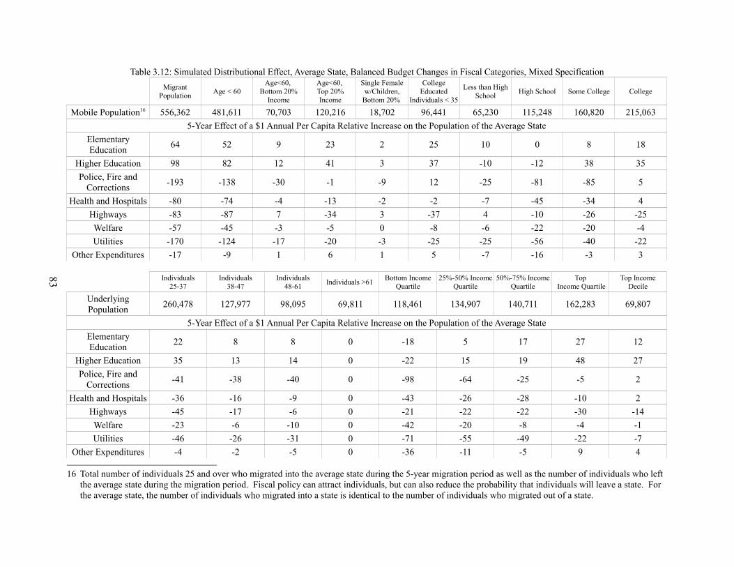
Table 3.12: Simulated Distributional Effect, Average State, Balanced Budget Changes in Fiscal Categories, Mixed SpecificationMigrant
Population Age < 60Age<60,
Bottom 20% Income
Age<60, Top 20% Income
Single Female w/Children,
Bottom 20%
College Educated
Individuals < 35
Less than High School High School Some College College
Mobile Population16 556,362 481,611 70,703 120,216 18,702 96,441 65,230 115,248 160,820 215,0635-Year Effect of a $1 Annual Per Capita Relative Increase on the Population of the Average State
Elementary Education 64 52 9 23 2 25 10 0 8 18
Higher Education 98 82 12 41 3 37 -10 -12 38 35Police, Fire and
Corrections -193 -138 -30 -1 -9 12 -25 -81 -85 5
Health and Hospitals -80 -74 -4 -13 -2 -2 -7 -45 -34 4Highways -83 -87 7 -34 3 -37 4 -10 -26 -25Welfare -57 -45 -3 -5 0 -8 -6 -22 -20 -4Utilities -170 -124 -17 -20 -3 -25 -25 -56 -40 -22
Other Expenditures -17 -9 1 6 1 5 -7 -16 -3 3
Individuals25-37
Individuals38-47
Individuals48-61 Individuals >61 Bottom Income
Quartile25%-50% Income
Quartile50%-75% Income
QuartileTop
Income QuartileTop Income
Decile
Underlying Population 260,478 127,977 98,095 69,811 118,461 134,907 140,711 162,283 69,807
5-Year Effect of a $1 Annual Per Capita Relative Increase on the Population of the Average StateElementary Education 22 8 8 0 -18 5 17 27 12
Higher Education 35 13 14 0 -22 15 19 48 27Police, Fire and
Corrections -41 -38 -40 0 -98 -64 -25 -5 2
Health and Hospitals -36 -16 -9 0 -43 -26 -28 -10 2Highways -45 -17 -6 0 -21 -22 -22 -30 -14Welfare -23 -6 -10 0 -42 -20 -8 -4 -1Utilities -46 -26 -31 0 -71 -55 -49 -22 -7
Other Expenditures -4 -2 -5 0 -36 -11 -5 9 4
16 Total number of individuals 25 and over who migrated into the average state during the 5-year migration period as well as the number of individuals who left the average state during the migration period. Fiscal policy can attract individuals, but can also reduce the probability that individuals will leave a state. For the average state, the number of individuals who migrated into a state is identical to the number of individuals who migrated out of a state.
83
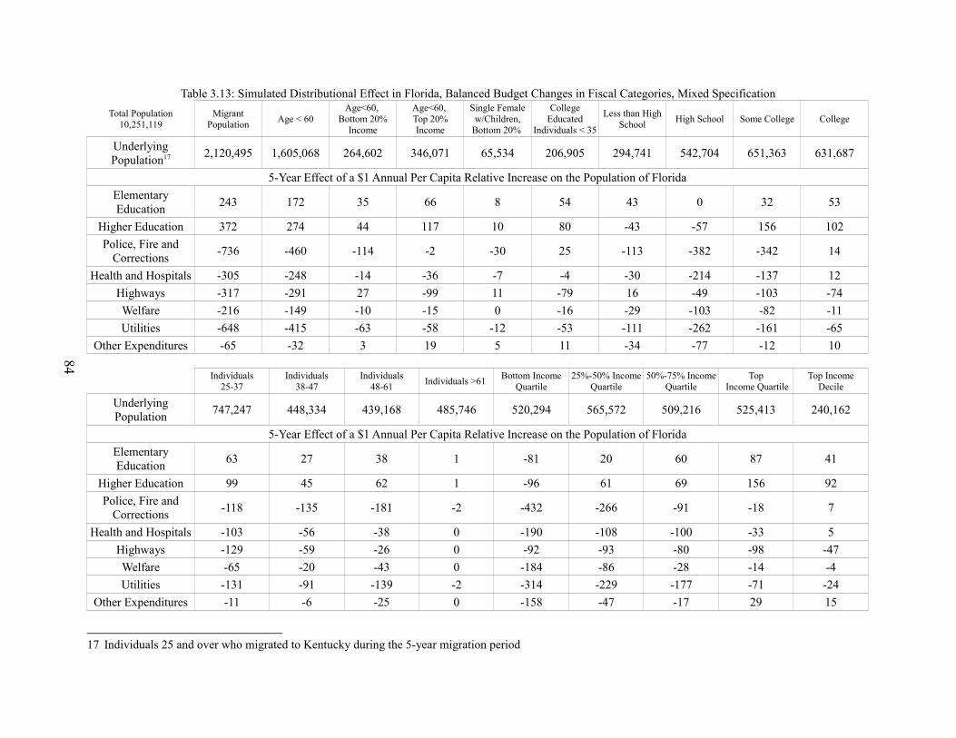
Table 3.13: Simulated Distributional Effect in Florida, Balanced Budget Changes in Fiscal Categories, Mixed SpecificationTotal Population
10,251,119Migrant
Population Age < 60Age<60,
Bottom 20% Income
Age<60, Top 20% Income
Single Female w/Children,
Bottom 20%
College Educated
Individuals < 35
Less than High School High School Some College College
Underlying Population17 2,120,495 1,605,068 264,602 346,071 65,534 206,905 294,741 542,704 651,363 631,687
5-Year Effect of a $1 Annual Per Capita Relative Increase on the Population of FloridaElementary Education 243 172 35 66 8 54 43 0 32 53
Higher Education 372 274 44 117 10 80 -43 -57 156 102Police, Fire and
Corrections -736 -460 -114 -2 -30 25 -113 -382 -342 14
Health and Hospitals -305 -248 -14 -36 -7 -4 -30 -214 -137 12Highways -317 -291 27 -99 11 -79 16 -49 -103 -74Welfare -216 -149 -10 -15 0 -16 -29 -103 -82 -11Utilities -648 -415 -63 -58 -12 -53 -111 -262 -161 -65
Other Expenditures -65 -32 3 19 5 11 -34 -77 -12 10
Individuals25-37
Individuals38-47
Individuals48-61 Individuals >61 Bottom Income
Quartile25%-50% Income
Quartile50%-75% Income
QuartileTop
Income QuartileTop Income
Decile
Underlying Population 747,247 448,334 439,168 485,746 520,294 565,572 509,216 525,413 240,162
5-Year Effect of a $1 Annual Per Capita Relative Increase on the Population of FloridaElementary Education 63 27 38 1 -81 20 60 87 41
Higher Education 99 45 62 1 -96 61 69 156 92Police, Fire and
Corrections -118 -135 -181 -2 -432 -266 -91 -18 7
Health and Hospitals -103 -56 -38 0 -190 -108 -100 -33 5Highways -129 -59 -26 0 -92 -93 -80 -98 -47Welfare -65 -20 -43 0 -184 -86 -28 -14 -4Utilities -131 -91 -139 -2 -314 -229 -177 -71 -24
Other Expenditures -11 -6 -25 0 -158 -47 -17 29 15
17 Individuals 25 and over who migrated to Kentucky during the 5-year migration period
84

Table 3.14: Simulated Distributional Effect in Nevada, Balanced Budget Changes in Fiscal Categories, Mixed SpecificationTotal Population
1,220,655Migrant
Population Age < 60Age<60,
Bottom 20% Income
Age<60, Top 20% Income
Single Female w/Children,
Bottom 20%
College Educated
Individuals < 35
Less than High School High School Some College College
Underlying Population18 454,403 375,464 60,628 71,050 15,085 31,927 76,519 123,092 158,247 96,545
5-Year Effect of a $1 Annual Per Capita Relative Increase on the Population of NevadaElementary Education 52 40 8 13 2 8 11 0 8 8
Higher Education 80 64 10 24 2 12 -11 -13 38 16Police, Fire and
Corrections -158 -108 -26 0 -7 4 -29 -87 -83 2
Health and Hospitals -65 -58 -3 -7 -2 -1 -8 -48 -33 2Highways -68 -68 6 -20 2 -12 4 -11 -25 -11Welfare -46 -35 -2 -3 0 -3 -8 -23 -20 -2Utilities -139 -97 -15 -12 -3 -8 -29 -59 -39 -10
Other Expenditures -14 -7 1 4 1 2 -9 -18 -3 2
Individuals25-37
Individuals38-47
Individuals48-61 Individuals >61 Bottom Income
Quartile25%-50% Income
Quartile50%-75% Income
QuartileTop
Income QuartileTop Income
Decile
Underlying Population 176,450 103,988 100,485 73,480 107,574 121,088 120,105 105,636 38,498
5-Year Effect of a $1 Annual Per Capita Relative Increase on the Population of NevadaElementary Education 15 6 9 0 -17 4 14 17 7
Higher Education 23 10 14 0 -20 13 16 31 15Police, Fire and
Corrections -28 -31 -41 0 -89 -57 -22 -4 1
Health and Hospitals -24 -13 -9 0 -39 -23 -23 -7 1Highways -30 -14 -6 0 -19 -20 -19 -20 -7Welfare -15 -5 -10 0 -38 -18 -7 -3 -1Utilities -31 -21 -32 0 -65 -49 -42 -14 -4
Other Expenditures -3 -1 -6 0 -33 -10 -4 6 2
18 Individuals 25 and over who migrated to Kentucky during the 5-year migration period
85

Table 3.15: Simulated Distributional Effect in Kentucky, Balanced Budget Changes in Fiscal Categories, Mixed SpecificationTotal Population
2,534,431Migrant
Population Age < 60Age<60,
Bottom 20% Income
Age<60, Top 20% Income
Single Female w/Children,
Bottom 20%
College Educated
Individuals < 35
Less than High School High School Some College College
Underlying Population19 357,550 316,221 59,277 58,250 16,596 50,899 51,771 87,777 105,541 65,203
5-Year Effect of a $1 Annual Per Capita Relative Increase on the Population of KentuckyElementary Education 41 34 8 11 2 13 8 0 5 5
Higher Education 63 54 10 20 2 20 -8 -9 25 11Police, Fire and
Corrections -124 -91 -25 0 -8 6 -20 -62 -55 1
Health and Hospitals -51 -49 -3 -6 -2 -1 -5 -35 -22 1Highways -53 -57 6 -17 3 -19 3 -8 -17 -8Welfare -36 -29 -2 -2 0 -4 -5 -17 -13 -1Utilities -109 -82 -14 -10 -3 -13 -20 -42 -26 -7
Other Expenditures -11 -6 1 3 1 3 -6 -12 -2 1
Individuals25-37
Individuals38-47
Individuals48-61 Individuals >61 Bottom Income
Quartile25%-50% Income
Quartile50%-75% Income
QuartileTop
Income QuartileTop Income
Decile
Underlying Population 170,467 83,370 65,837 37,886 92,718 95,433 88,844 80,565 30,449
5-Year Effect of a $1 Annual Per Capita Relative Increase on the Population of KentuckyElementary Education 15 6 6 0 -17 3 11 13 5
Higher Education 23 9 10 0 -20 10 12 24 12Police, Fire and
Corrections -27 -28 -30 0 -90 -45 -16 -3 1
Health and Hospitals -24 -12 -6 0 -40 -18 -18 -5 1Highways -30 -12 -4 0 -19 -16 -14 -15 -6Welfare -15 -4 -7 0 -38 -15 -5 -2 -1Utilities -30 -19 -23 0 -66 -39 -32 -11 -3
Other Expenditures -3 -1 -4 0 -33 -8 -3 4 2
19 Individuals 25 and over who migrated to Kentucky during the 5-year migration period
86

Chapter 4: Heterogeneity and Government Involvement in the Economy
While migration provides individuals an opportunity to “vote with their feet,”
there are a limited number of jurisdictions for individuals to migrate to and some
individuals will not be completely satisfied with the size and scope of the public sector.
Some individuals will demand greater levels of provision, while others will demand less,
and some preference heterogeneity will remain within jurisdictions.
Throughout history, heterogeneity has generated violent conflict, especially when
preferences differ (or at least are perceived to differ) along ethnic and/or cultural lines.
Perpetual ethnic conflict in the Balkans and the Caucasus provide a constant reminder.
Fearon and Laitin (1996) point out that interethnic cooperation is actually more common
than conflict primarily because individuals fear that any conflict between ethnic groups
can quickly spiral out of control. This provides strong incentives to avoid disputes, and
allows a heterogeneous population to exist in a stable long run equilibrium.
Page (2007) explains how individuals with different backgrounds and experiences
can enhance the ability of organizations to solve problems. On the other hand, Hall and
Leeson (2010) find evidence that students in heterogeneous schools have lower test
scores. Putnam (1995) points out that heterogeneous groups are less likely to trust and
cooperate with one another. Easterly and Levine (1997) and Zak and Knack (2001) find
an inverse relationship between heterogeneity and economic growth.
German Chancellor Angela Merkel claimed in Der Spiegel on October 16, 2010
that the German approach to multiculturalism has “absolutely failed,” and that
immigrants must begin to adopt the German language and culture. Schuck (2003)
87

suggests that government activity should be restricted to promoting tolerance and
preventing discrimination, since attempts to promote multiculturalism are unlikely to do
anything but increase ethnic tension. Similarly, Leeson (2007) suggests that interethnic
cooperation arises spontaneously, and government efforts to promote this cooperation can
be counterproductive.
In addition to affecting productivity in the private sector, the level of intergroup
cooperation and preference heterogeneity can also affect the public sector. Olson (1965)
suggested that the costs of coming to a group consensus increases with the number of
competing interests. Dahl and Tufte (1973) theorize that preference heterogeneity
produces a greater relative number of competing minority groups. If a consensus is
required for new policies to be implemented in a democracy, then an inverse relationship
between the number of minority groups and government size could result.
Cutler et al (1993) introduce this idea as the “community preference model,” and find
that preference for public provision may depend on an individual's similarity to others
within the jurisdiction. Under this model, greater levels of provision should be expected
in homogeneous jurisdictions.
Alesina and Spolaore (1997) present a formal model of country formation that
suggests a tradeoff between heterogeneity and country size. Large countries tend to have
larger populations and benefit from economies of scale in public provision. Large
countries also suffer from increased preference heterogeneity, as transactions costs are
higher and citizens are less likely to agree on the role of government in the economy.
88

These ideas have been tested empirically. Many studies have documented a
relationship between certain types of spending and heterogeneity. Easterly and Levine
(1997) find that ethnic diversity is inversely related to educational attainment and
infrastructure. LaPorta et al (1999) find that ethnic diversity is associated with
government corruption, regulation, and a lack of property rights. They find that
budgetary government size is inversely related to heterogeneity, and heterogeneous
countries are more likely to have governments that perform poorly. Alesina et al (1999)
find an inverse relationship between ethnic heterogeneity and government spending on
education, roads, sewers and sanitation among a sample of US metropolitan areas. Kuijs
(2000) finds that ethnic heterogeneity is inversely related to health and education
outcomes for a sample of countries from 1980.
Other empirical studies have documented an inverse relationship between
heterogeneity and levels of trust and cooperation, which would imply that heterogeneous
groups would demand less public provision. In one of the most interesting studies, Costa
and Kahn (2003a) find that Union Army soldiers who served in the Civil War and were
from fragmented jurisdictions or were serving in fragmented units were significantly
more likely to desert, be arrested, or go AWOL. Costa and Kahn (2003b) find that an
increase in fragmentation from the mid 1970s to 1990 reduces the probability of
volunteering and group membership for older Americans. Poterba (1997) and Goldin and
Katz (1999) find an inverse relationship between education spending and heterogeneity,
consistent with the idea that individuals care more about the education of members of
their own group. Swee (2010) finds that political partitioning from the 1992-1995
89

Bosnian War tended to homogenize the region. As a result, ethnic majorities experienced
an increase in the provision of education while ethnic minorities did not. Luttmer (2001)
finds that support for welfare spending in an area is higher among those living in areas
with larger percentages of individuals from the their own ethnic group. Vigdor (2004)
finds a lower census response rate in fragmented counties, consistent with the idea that
individuals in these areas have a lower sense of civic duty and are less likely to
cooperate. Alesina and LeFerrara (2002), Leigh (2006a, 2006b), and Putnam (2007) find
an inverse relationship between heterogeneity and survey measures of trust.
The mechanism behind this relationship seems obvious. In democracies, elections
link demand for public provision to actual provision levels. Under the assumption that
self-interested politicians attempt to extract rent from the voting base, there are relatively
few opportunities to do so, since unpopular politicians are easily removed from office.
However, these constraints do not apply in non-democratic countries, and relationships
between government spending and heterogeneity are less obvious. Leaders have different
levels of political control, and this control is affected by the number of competing citizen
groups. Heterogeneous populations may prefer less government, but if heterogeneity also
affects the relationship between preferences and actual provision, the net effect of
heterogeneity is uncertain.
In general, groups in non-democratic countries will affect political outcomes if
they have grievances and the opportunity to exert pressure on the state (Sorens, 2010). In
order to “appease” the group, leaders can either address the grievances or attack the
group's ability to exert political pressure. For the leader, the former act is costly since
90

resources spent on the group's demands are no longer available to be captured as rent.
The latter act is costly in the sense that political capital is spent whenever coercion is
used on the population, and this increases the probability of a leadership change. On the
other hand, the latter act may yield benefits in terms of additional opportunities to extract
rent in the future.
In unstable countries where a monopoly on violence has not developed,
“governments” can closely resemble violent non-state actors and resort to highly
repressive acts in order to establish and maintain control. Countries such as Afghanistan,
Chad, Somalia and Sudan provide contemporary examples.
McGuire and Olson (1996) theorize that it is in everyone's best interest for one
“bandit” to eventually monopolize theft, as a symbiotic relationship is formed between
the bandit and the victims. The bandit has an incentive to limit their extraction of rent
and provide some goods in order to secure future payments. A similar idea was
introduced earlier by Mises (1957), who suggested that public opinion controls public
policy in democracies as well as in dictatorships, as dictators must remain popular
enough to stay in power (Caplan, 2008).
However, in heterogeneous societies with competing interests, “public opinion” is
not well-defined, and would be less likely to constrain the actions of a dictator.
Successful dictators in these countries commonly use a “divide-and-rule” political
strategy to maintain power (Acemoglu, Robinson, and Verdier, 2004). Under this
strategy, the ruler does not necessarily appease all groups, but must ensure that groups do
not form the cooperative coalitions necessary to mount a successful challenge. As the
91

population becomes more fragmented, leaders face fewer constraints.
Weingast's (1995) sovereign-constituency transgression game can be extended to
illustrate this point. In order for a citizen to support the sovereign, the sovereign cannot
transgress that citizen's rights. While this is necessary to retain that citizen's support, it is
not sufficient, and citizens can still choose to oppose the sovereign. A certain percentage
of the population must be appeased, or else the sovereign loses power.
A simplified specification suggests that there are only two groups, and the
sovereign can transgress against one, both, or none of the groups. The groups move next,
and can choose to incur a cost and challenge the sovereign, even if the sovereign has not
transgressed. If both groups challenge, then the sovereign loses power. If only one group
challenges, then the challenge fails and the sovereign's transgressions are successful.
Because this is a repeated game, the folk theorem dictates that groups have
incentives to cooperate. If one group defects and allows the sovereign to exploit the other
it can be punished in a future game if the other group decides to reciprocate. In the event
that one group decides to challenge the sovereign, the other group will also challenge if
the gains from removing the sovereign from power exceed the costs of challenging.
Under this scenario, the sovereign has strong incentives to appease at least one group
(i.e., half of the population) in order to remain in power.
If Weingast's model is modified by allowing additional (more than two) groups,
these incentives may be reduced. Heterogeneous societies consist of larger numbers of
groups that are less interested about the welfare of other groups. In these societies it
would be more costly for multiple groups to organize and form a coalition. Ceteris
92

paribus, the sovereign can choose to transgress the rights from small groups with relative
impunity. Due to a “Niemoller Effect,” they may find it easier to single out and extract
resources from small groups. Individuals are less likely to object if they are not a
member of the group that the dictator is currently extracting rent from. In addition,
dictators can consolidate their power by paying rent to a small loyal subgroup of
“kingmakers” who are members of the same ethnic group in order to maintain hegemonic
control over the other groups (Gallego and Pitchik, 2004). Acemoglu et al (2007) show
that the presence of raw materials and foreign aid tend to increase this power, as both
provide resources that despots can use to placate opposition. They also state that low
levels of average productivity in the economy give kleptocrats more freedom to extract
rent.
Dictators in homogeneous countries are more likely to be constrained by public
opinion. Autocratic rulers do not necessarily have to provide productive goods, but they
likely do have to take some actions in an attempt to address public opinion. These
actions do not necessarily include productive public provision. Investments in mass
media, for example, can be used to increase the level of power held by the sovereign
(Debs, 2007). Some manage to establish a personality cult and directly manipulate public
opinion by fiat.
There are relatively few studies on government activity in these non-democratic
countries. This is partly because data is misleading. Schneider and Enste (2000) find that
developing countries have significantly larger shadow economies. Similarly, Dreher et al
(2007) show that poor government institutions appear to reduce the size of the economy,
93

but only because a significant portion of economic activity is being driven underground.
Johnson et al (1997) find that bribes and other forms of corruption act as substitutes for
official taxation, and are used to extract resources from the shadow economy in much the
same way that taxes can from the official economy. Studies that examine the size of
government in developing countries must control for these alternative forms of
intervention.
94

Chapter 5: Heterogeneity, Political Rights and the Public Sector
This study empirically explores the relationships between heterogeneity and the
public sector. Measures of ethnic heterogeneity are compared to various measures of
government intervention in the economy in order to determine the extent of the
relationship. While previous studies generally find an inverse relationship, this study
differs in that it assumes that these relationships depend upon the level of political rights
in a jurisdiction. Citizens are thought to have relatively more political power in
democracies, therefore changes in provision and government activity in these countries
will reflect the will of the underlying population. In countries where actions taken by
leaders are not subject to the same level of citizen scrutiny, government activity is less
likely to reflect the will of the population. If heterogeneous groups do prefer lower levels
of government activity, then inverse relationships should be more apparent in
democracies.
This study also differs from previous research by including non-budgetary forms
of government intervention in the analysis. In developing countries, conventional taxes
would fall on a relatively small base. This is because these countries have large
underground “shadow” economies. A large portion of economic activity may happen on
the black market, where individuals are paid cash in exchange for goods and services, and
there would be relatively little incentive to comply with income and/or sales tax
legislation. In other cases, individuals barter for goods and services, and this activity
would not be difficult to tax. Governments in these developing countries must rely on
other methods to extract the resources needed to finance operations. In some cases,
95

government officials elicit bribes as payment for their services. In other cases, property
is not well defined, and can be taken for public use. As previous studies focus primarily
on fiscal policy, they exclude countries with relatively large shadow economies that rely
on conventional taxation to a lesser extent.
In order to examine these relationships, the effect of ethnic heterogeneity on
measures of budgetary and non-budgetary government is estimated for a large panel of
countries. A limitation of this study is that cultural and political institutions can differ
widely between countries. Comparisons of countries placed into the categories of
dictatorships and democracies are not straightforward and may oversimplify these
differences.
Data
Data was taken from a variety of sources. The most common index of
heterogeneity used in recent literature is that constructed by Alesina et al (2002). This
index contains measures of ethnic, linguistic, and religious fractionalization for 215
countries and territories. These variables represent the probability that two randomly
selected individuals are from different groups, and are calculated according to equation
(5.1) below.
1−∑i
racei2
(5.1)
These probabilities are assumed to remain constant over time for each country.
Table 5.2 lists 2007 GDP per capita and information on notable historical figures for the
25 countries with the highest levels of ethnic fractionalization. With the exception of
96

Qatar, each of these countries has a recent history of conflict. In almost all cases, control
of the country was won through a military coup. In some cases, leaders were able to
maintain a large degree of political power and control the country for an extended period
of time. In other cases, leadership changed hands a number of times over a very short
period of time.
Table 5.3 lists the 25 countries with the lowest levels of ethnic fractionalization.
With few exceptions, these countries have relatively high levels of economic
development and are more likely to have democratic governments. The average level of
GDP per capita in 2007 for the most homogeneous countries is $14,281 higher than the
most heterogeneous countries. Homogeneity also appears to reduce conflict and increase
the level of stability in a country. However, the tendency of individuals in homogeneous
groups to be less suspicious of and less likely to question the actions of others can
backfire in certain cases.
North Korea is one of the most homogeneous countries in the world, and the only
homogeneous country to remain under the control of a dictator. Individuals are immersed
in propaganda at a young age, and are taught that they are members of a superior race,
and that their leaders (i.e., Kim Il Sung, Kim Jong Il and Kim Jong Un) exhibit the
highest level of moral, cultural, and genetic purity. Individuals monitor each other and
report any behavioral infractions to the authorities. Those suspected of violations are
sent, along with their families, to forced-labor camps. The stability of the North Korean
regime depends on this race-based nationalism (Myers, 2010).
François “Papa Doc” Duvalier is another relatively well-known despot who
97

maintained a highly repressive regime in Haiti until his death in 1971. He cultivated his
reputation as a voodoo priest to maintain control over a homogeneous population with an
overarching belief system. A personality cult was established by the dictators in both
North Korea and Haiti. Both leaders managed to convince the population to support their
autocratic rule. This may have been more difficult with a heterogeneous population.
Tables 5.2 and 5.3 suggest that heterogeneous countries are generally more likely
to be ruled by dictators, though perhaps less likely to be considered personality cults.
Table 5.4 presents a list of countries of notable historical significance for comparison.
Augusto Pinochet is notable because he managed to maintain control of a relatively
homogeneous Chile for over 25 years without establishing a personality cult. Relatively
high levels of economic growth may have contributed to political stability in this case.
Table 5.4 also suggests that some of the world's most famous dictators ruled
countries with average levels of heterogeneity. Among these are Fidel Castro, Nicolae
Ceauşescu, Francisco Franco, Saddam Hussein, and Manuel Noriega. One of the most
interesting characters is Saparmurat Niyazov of Turkmenistan, also known as
“Turkmenbashi the Great.” Niyazov is notable for renaming airports, cities, calendar
months, and passing meteorites after himself and family members, writing spiritual
guidebooks, and building large gold-plated statues of himself, one of which would rotate
to always face the sun. He is also known for political purges, a 60 percent unemployment
rate, and the closure of all hospitals outside the capital city, as they were deemed to be
unnecessary (Steyn, 2007).
While the U.S. has a reputation as a “melting pot,” the level of ethnic
98

heterogeneity is 0.49, which is lower than those countries in Table 5.2. This is partly due
to the way that ethnic groups are defined across countries. Ethnicity in the U.S. is
primarily determined by race, though it is determined by other characteristics, such as
tribal affiliation in many other countries. Due to the relatively large number of groups,
some of these countries are considered to be more heterogeneous than the U.S.
From these tables, an inverse relationship between heterogeneity and political
rights is apparent. Lower levels of GDP per capita provide evidence that these
heterogeneous countries also have lower levels of economic development. However, the
shadow economy must be also considered. While it seems unreasonable that individuals
in Liberia, Somalia, and the DRC can survive on less than $500 per year, it is likely that
most of these individuals produce a significant portion of their income via shadow wages.
Government interference in the economy in these cases will be fundamentally different
than in developed countries.
In order to measure non-budgetary government interference in the economy, data
was collected from the Fraser Institute's Economic Freedom of the World Index. This
dataset provides annual information on countries in each of 5 areas that include budgetary
government, legal environment, integrity of the monetary base, freedom to trade
internationally, and business freedom. This study emphasizes the legal environment and
business freedom, as these areas most closely represent non-budgetary government
activities that can act as “shadow taxes.”
The legal environment represents a composite of similar scores for individual
categories such as judicial integrity, military influence in the courts, and restrictions on
99

the sale of private property. Scores in these individual categories are generated from
various sources. One of these is the World Economic Forum's Global Competitiveness
Report. This report is generated from responses to surveys that are administered to
approximately 13,000 business executives worldwide. Respondents were asked to rate
their country's legal institutions on a scale of 1 to 7 with specific questions asked about
subtopics including legal protection of property rights, the independence of the judiciary,
and the ability of private businesses to challenge the legality of government actions in
court.. Another source used to calculate the legal environment score is the PRS Group's
International Country Risk Guide. This index produces risk scores using a proprietary
econometric model. A third source is the World Bank's Doing Business index, which
provides cross-sectional comparisons of the costs and time required to undertake
activities associated with running a private business. Activities included in this index are
the legal registration of property and the ability to enforce contracts.
Values for the Economic Freedom of the World's business freedom area represent
a similar composite of measures of credit restrictions and business regulations. Scores in
this area were also constructed from categories within the World Bank's Doing Business
index such as minimum wages, accessibility of credit, mandated costs of hiring and firing
workers, and licensing restrictions. In addition, survey response categories from the
Global Competitiveness Report were included in areas such as bribes, administrative
regulations, costs of dealing with bureaucracy, and the determination of wages through
collective bargaining.
Population data was taken from the World Bank's 2010 World Development
100

Indicators, and GDP per capita was taken from the Penn World Table. Values for GDP
per capita in 2008 were imputed using a Box-Jenkins ARMA model.
Political rights are measured using Freedom House's Gastil Index. This is a 7
point score that represents the level of political rights in each country. Autocratic
countries that received a 6 or 7 (the two lowest scores) in 2008 are listed in Table 5.5,
while Table 5.6 lists the democratic countries that received a score of 1, indicating the
highest level of political rights. Though there is an inverse relationship between
heterogeneity and political rights, there is a positive relationship between budgetary
government and political rights. Countries with low political rights also have lower
levels of legal or business rights. In many of the cases where government data is
unavailable (i.e., North Korea, Somalia, Sudan), it is obvious that few legal or business
freedoms exist.
Table 5.1 provides summary statistics and correlation tables for each of the
measures of government activity broken down by the level of political rights. Countries
with lower levels of political rights have lower levels of budgetary government, but
higher levels of non-budgetary activity. Because the measures of non-budgetary
government activity are based on a 1-10 scale, with 1 being the highest and 10 being the
lowest level of government activity, positive correlations between budgetary and non-
budgetary measures suggest that the actual activities are inversely related. All categories
of non-budgetary government activity are therefore inversely related to budgetary
activity. This is consistent with Boettke (2001) and Brennan's (2002) suggestion that
“subsidy and regulation are alternative technologies for securing the same policy
101

objective is familiar to those who make international comparisons of public sector size.”20
From the correlation tables, heterogeneity is inversely related to budgetary
government in countries with high levels of political rights. Heterogeneity is positively
related to non-budgetary government in countries with low levels of political rights.
Heterogeneity is inversely related to government ownership of private industry in
democracies, and restrictions on the sale of private property is positively associated with
heterogeneity in countries with low political rights. Also consistent with this finding, the
freedom to operate private business is positively associated with heterogeneity in
countries with high political rights, but not in other countries.
Results
The central contribution of this chapter is to document the relationship between
heterogeneity and government in countries with low levels of political rights, while
considering the fact that these countries may rely heavily on shadow taxes to “finance”
activity. Table 5.7 presents results of a random-effects model that is estimated for each of
the three measures of government activity by level of political rights for a panel of 139
countries from 2005-2008. Heterogeneity is found to have a strong negative effect on
budgetary governments in democracies, consistent with predictions in the literature.
Heterogeneity is also found to have a positive effect on the level of business freedom in
democracies.
Other than transfer payments, heterogeneity has little effect on budgetary
government in non-democratic countries. Heterogeneity is positively related to non-
budgetary government in non-democratic countries. If heterogeneity has no effect on
20 p.21
102

budgetary government, but is found to positively affect non-budgetary government, then
heterogeneity will have an overall positive relationship with government size in non-
democratic countries. This is consistent with theories by Sorens (2010) that suggest that
official ethnic discrimination depends upon political institutions.
For this sample, a fixed-effects specification was also estimated with
heterogeneity absent from the model. Hausman tests were performed to examine the
extent to which country-specific characteristics impact these results. In most cases,
results from fixed effects specifications were not significantly different from the random
effects specification. One notable exception is transfer payments, where estimates
produced with fixed and random effects specifications differ regardless of the level of
political rights. In addition, there are significant differences between fixed and random
effects estimates for budgetary government measures in democracies. In these cases,
countries likely have unique characteristics that explain fiscal policy in addition to those
being captured by the random effects specifications.
One concern is that splitting the data by the level of political rights introduces
endogeneity. If countries that have lower levels of political rights also have lower levels
of legal and economic rights, then the effect of heterogeneity may be biased. In addition,
bias will be introduced if the level of GDP per capita depends upon the level of
government intervention in the economy. This is likely if individuals reduce their
economic activity or move activity into a shadow economy in response to taxation. In
this case, estimates of the effect of GDP per capita on the level of government
involvement in the economy would be downwardly biased. More importantly, this biases
103

estimates of the effect of heterogeneity on government. Ideally, instruments could be
found to proxy for the initial value of GDP per capita. However, the availability of
reliable instruments is limited, especially for such a large panel of countries.
Table 5.8 presents the results of a random effects specification that omits GDP per
capita. In most cases, the estimated coefficients on ethnic heterogeneity are more
negative than those found in Table 5.7. This suggests that the estimates in Table 5.7 tend
to understate the effect of heterogeneity on government involvement in the economy.
Another concern is that the level of political rights in countries does not vary
much over time between 2005 and 2008. To address this, a larger panel of data is
constructed for 122 countries dating back to 1985 from the same sources. Due to the
limitations of the Economic Freedom of the World dataset, observations are included
once every 5 years for 1985, 1990, 1995, and 2000. Annual data exists from 2000
through 2008. Some countries, such as former members of the Soviet Union have no
observations prior to 1995. Values for population, GDP per capita, or budgetary
government values were imputed for countries that were missing one observation for one
of these variables. Data limitations exclude the categories of government enterprises and
investment, and legal restrictions on the sale of private property in this sample.
Included in this larger sample are countries that experienced significant changes
in political rights over time. Some of these, such as Albania, Hungary, Poland, and
Romania, transitioned from a communist government to a democracy after the fall of the
Iron Curtain. From 1985 to 1990, the average level of budgetary government activity in
these countries jumped from an average of 28.8% of GDP to 45.67% of GDP. Over the
104

same period of time the level of legal and property rights rose from 5.6 to 7.1, suggesting
non-budgetary government intervention in the economy fell.
Table 5.9 provides the average values for budgetary government, population, and
real gross national income per capita measures for each of the 122 countries in this larger
sample. Table 5.10 provides summary statistics and correlations. Heterogeneity is
inversely correlated with budgetary government and positively correlated with non-
budgetary government regardless of the level of political rights. Table 5.11 presents
results from a random effects model estimated for this larger panel. Results are generally
similar. In all cases, heterogeneity is inversely related to transfer payments.
Heterogeneity is only inversely related to budgetary government consumption in
democracies with high political rights. The inverse relationship between heterogeneity
and total budgetary government is approximately 10 percentage points higher in
democracies, primarily because of the effect on government consumption.
Heterogeneity is found to have an inverse effect on legal and property rights.
While the effect is of larger magnitude in countries with low political rights, and
heterogeneity may have a larger effect on non-budgetary government activity in non-
democratic countries, the result for democracies is unexpected. Perhaps additional legal
measures are needed to reduce conflict, or special interest lobbying in heterogeneous
democracies produces higher levels of intervention. Perhaps the legal system is more
developed in democracies and therefore produces lower scores on the surveys used to
generate the legal environment variable. In addition, survey responses may take time to
change while information on political institutions changes instantaneously with
105

institutional changes. Because of this, transitional economies may continue to receive
low survey scores for years after becoming a democracy.
While the effect of heterogeneity in democracies on legal freedom is negative in
both panels, it is only significant in the larger panel. Similarly, the effect of heterogeneity
in democracies on business freedom is positive in both panels, but only significant in the
smaller panel. Because of the subjective nature of non-budgetary measures, the net effect
of heterogeneity on overall government size in democracies remains unclear.
In non-democratic countries, heterogeneity does not reduce government
consumption, but does increase regulation and non-budgetary interference in the
economy. If transfer payments are excluded, the net effect of heterogeneity in this case is
to increase the overall size of government. It is interesting to note that in both Table 5.7
and Table 5.11, positive relationships between government consumption and GDP per
capita are consistent with “Wagner's Law.”
Conclusion
This chapter explores the relationships between heterogeneity and government
size. Inverse relationships between budgetary government consumption and transfer
payments are confirmed, at least for democracies. This is consistent with prior research
that suggests that heterogeneity of preferences reduces public provision and individuals
have less taste for redistribution in heterogeneous communities.
This study considers non-budgetary government as well, as developing countries
with large shadow economies frequently rely on regulation and other forms of
intervention in the economy. When these alternative forms of government are
106

considered, the standard relationship between heterogeneity and government size does
not hold. This study finds that the relationship may depend upon the level of political
rights.
Perhaps individuals in heterogeneous groups do prefer lower levels of public
provision. However, in non-democratic countries, preferences for government activity do
not necessarily materialize. No relationship between budgetary government consumption
and heterogeneity is found for these non-democratic countries, though a positive
relationship between non-budgetary government and heterogeneity is found.
In democratic countries, an inverse relationship between heterogeneity and
budgetary consumption is found. Unexpectedly, a positive relationship between
heterogeneity and non-budgetary intervention through the legal system is also found for
democratic countries, though this may be due to the way the variable is constructed. In
general, heterogeneity does reduce the size of budgetary government, but the effect of
heterogeneity on regulation and economic freedom is not clear.
107

Table 5.1: Summary Statistics, 2008 (N=139)
VariableMeans by Level of Political Rights
Low Political Rights Med Political Rights High Political Rights
Government Consumption(% of GDP) 20.96 17.13 24.34
Transfer Payments (% of GDP) 4.22 6.02 15.51
Total Government (% of GDP) 25.18 23.15 39.85
Government-Owned Enterprises 3.8 5.4 8.6
Legal and Property Rights 4.9 4.9 7.2
Freedom to Transfer Property 6.9 6.9 7.8
Business Freedom 6.2 6.7 7.3
Population (millions) 80.5 46.3 25.0
Real GDP Per Capita (2008 US$) $6,725.7321 $5,831.35 $22,276.24
Ethnic Heterogeneity 0.51 0.54 0.26
Correlations Between Measures of Government Activity
Total Budgetary Government
Government Enterprises
Legal and Property Rights
Freedom to Transfer Property
Government Enterprises 0.37***
Legal and Property Rights 0.62*** 0.47***
Freedom to Transfer Property 0.26*** 0.23*** 0.56***
Business Freedom 0.25*** 0.37*** 0.63*** 0.38***
VariableCorrelations with Ethnic Heterogeneity by Level of Political Rights
Low Political Rights Med Political Rights High Political Rights
Government Consumption(% of GDP) -0.01 -0.05 -0.30***
Transfer Payments (% of GDP) -0.62*** -0.12 -0.43***
Total Government (% of GDP) -0.22 -0.10 -0.42***
Government-Owned Enterprises -0.03 -0.29** -0.31**
Legal and Property Rights -0.66*** -0.09 -0.26*
Freedom to Transfer Property -0.73*** -0.21* 0.00
Business Freedom -0.15 -0.14 0.30*
Population (millions) -0.30 -0.05 0.02
Real GDP Per Capita (2008 US$) -0.10 -0.18 -0.11***
21 Oman and UAE have relatively high GDP per capita.
108

Table 5.2: Heterogeneous CountriesCountry Fractionalization GDP Per Capita22 Notable Figures
Uganda 0.93 $1,299 Idi Amin (1971-1979)*Yoweri Museveni (1986- )
Liberia 0.91 $409 Samuel Doe (1980-1990)*Charles Taylor (1990?-2003)*
Madagascar 0.88 $918 Didier Ratsiraka (1975-1993, 1997-2002)*DRC (Zaire) 0.87 $414 Mobuto (1965-1997)*Congo-Brazzaville 0.87 $3,965 Denis Sassou Nguesso (1979-1992, 1997- )*Cameroon 0.86 $2,938 Paul Biya (1982- )*Chad 0.86 $2,830 Idriss Déby (1990- )*Kenya 0.86 $2,191 Daniel arap Moi (1978-2002)*
Nigeria 0.85 $2,520
Yakubu Dan-Yumma Gowon (1966-1975)*Murtala Ramat Mohammed (1975-1976)*Olu ẹgun Ọbasanjọ (1976-1979, 1999-2007)*ṣSani Abacha (1993-1998)*
CAR 0.83 $924 Jean-Bédel Bokassa (1966-1979)*François Bozizé (2003- )*
Cote d'Ivoire 0.82 $2,377 Félix Boigny (1960-1993)*Sierra Leone 0.82 $1,988 Siaka Stevens (1967-1985)*
Somalia 0.81 $491Mohamed Siad Barre (1969-1991)*Mohamed Farrah Aidid (1995-1996)*Hussein Mohamed Farrah (1996-1997)
Yugoslavia 0.81 N/A Josip Broz Tito (1953-1980)*Slobodan Milošević (1989-2000)*
Guinea-Bissau 0.81 $658 Luís Cabral (1973-1980)João Vieira (1980-1999, 2005-2009)*
Djibouti 0.80 $4,650 Hassan Aptidon (1977-1999)*Libya 0.79 $24,281 Mu'ammar Al-Qadhafi (1969- )*Benin 0.79 $1,491 Mathieu Kérékou' (1972-1991)*Angola 0.79 $5,449 José Eduardo dos Santos (1979- )*Gambia 0.79 $1,554 Yahya Jammeh (1994- )*Zambia 0.78 $2,297 Kenneth Kaunda (1964-1991)*Afghanistan 0.77 $797Gabon 0.77 $9,179 Omar Bongo (1967-2009)*South Africa 0.75 $11,307Qatar 0.75 $104,707 Sheikh Hamad bin Kalifa Al Thani (1995- )Average - $7,901* leaders who seized power in a military coup or imposed legal restrictions on political competition.
22 Penn World Table, 6.3
109

Table 5.3: Homogeneous CountriesCountry Fractionalization GDP Per Capita Notable FiguresComoros 0.00 $1,808.31 Bob DenardSouth Korea 0.00 $24,949.65Japan 0.01 $32,063.24
North Korea 0.04 $1,900.00 (est.) Kim Il Sung (1972-1994)*Kim Jong Il (1994- )*
Tunisia 0.04 $10,641.26 Zine El Abidine Ben Ali (1987- )*Vanuatu 0.04 $5,929.65Malta 0.04 $23,006.44Bangladesh 0.05 $2,470.90 Sheikh Mujibur Rahman (1972-1975)*Portugal 0.05 $21,526.84 António de Oliveira Salazar (1932-1968)*Kiribati 0.05 $1,915.07Swaziland 0.06 $7,746.05 King Mswati III (1986- )Norway 0.06 $53,964.52Sweden 0.06 $35,270.78Marshall Islands 0.06 $7,649.58Iceland 0.08 $40,907.56Denmark 0.08 $36,198.32Tonga 0.09 $6,075.81 King Tāufa āhau Tupou IV (1965-2006)ʻAustralia 0.09 $39,694.06Cyprus 0.09 $26,780.39Haiti 0.10 $1,669.38 François (“Papa Doc”) Duvalier (1957-1971)*France 0.10 $31,446.69Netherlands 0.11 $36,394.13Austria 0.11 $38,302.66Italy 0.11 $30,505.24Poland 0.12 $15,447.54Average - $22,182* leaders who seized power in a military coup or imposed legal restrictions on political competition.
110

Table 5.4: Other Notable CountriesCountry Fractionalization GDP Per Capita Notable Figures
Cape Verde 0.42 $8,266.29 Aristides Pereira (1975-1991)*
Chile 0.19 $21,548.43 Augusto Pinochet (1974-1990)*
Cuba 0.59 $11,762.46 Fulgencio Batista (1940-1944, 1952-1959)*Fidel Castro (1959-2008)*
Equatorial Guinea 0.35 $17,680.07 Teodoro Obiang Nguema Mbasogo (1979- )*
Guinea 0.74 $3,794.40Lansana Conté (1984-2008)*Moussa Dadis Camara (2008-2009)*Sékouba Konaté (2009- )*
Ethiopia 0.72 $1,203.68 Meles Zenawi (1991- )*
Indonesia 0.74 $5,468.30 Suharto (1967-1998)*
Iraq 0.37 $5,103.17 Saddam Hussein (1979-2003)*
Mozambique 0.69 $2,306.26 Samora Machel (1975-1986)*
Panama 0.55 $9,480.51 Manuel Noriega (1983-1989)*
Romania 0.31 $10,506.91 Nicolae Ceauşescu (1965-1989)*
Rwanda 0.32 $1,216.32 Juvénal Habyarimana (1973-1994)*
São Tomé & Príncipe N/A $5,020.66 Manuel Pinto da Costa (1975-1991)*
Spain 0.42 $33,615.80 Francisco Franco (1939-1975)*
Sudan 0.71 $2,569.71 Gaafar Nimeiry (1969-1985)*Omar Hasan Ahmad al-Bashir (1989- )*
Tanzania 0.74 $944.89 Julius Nyerere (1964-1985)*
Togo 0.71 $951.65 Gnassingbé Eyadéma (1967-2005)
Turkmenistan 0.39 $12,118.94 Saparmurat Niyazov (1990-2006)*
United States 0.49 $45.597.07
Zimbabwe 0.39 $2,448.50 Robert Mugabe (1987- )** leaders who seized power in a military coup or imposed legal restrictions on political competition.
111

Table 5.5: Countries With Low Political Rights, 2008
Country Ethnic Heterogeneity
Budgetary Government Legal Rights Business
FreedomAlgeria 0.34 43.32% 4.5 5.2Angola 0.79 45.48% 3.3 5.1Armenia 0.13 22.44% 5.5 6.8Azerbaijan 0.20 26.99% 6.4 6.9Cambodia 0.21 - - -Cameroon 0.86 19.60% 3.5 6.4Congo, Rep. Of 0.87 28.48% 2.9 5.7Cote d'Ivoire 0.82 12.06% 3.1 6.1DRC (Zaire) 0.87 13.01% 2.1 4.3Egypt 0.18 24.94% 5.4 5.6Fiji 0.55 30.84% 6.0 8.8Gabon 0.77 21.14% 4.3 6.9Iran 0.67 27.15% 6.1 5.4Iraq 0.37 - - -Kazakhstan 0.62 26.18% 6.0 7.5Mauritania 0.62 23.19% 4.7 7.2Oman 0.44 32.16% 7.4 7.9Qatar 0.75 - - -Russia 0.25 39.59% 5.7 5.9Rwanda 0.32 13.22% 5.8 7.4Tajikistan 0.51 - - -Unit. Arab Em. 0.63 18.54% 7.2 7.6Belarus 0.32 - - -Chad 0.86 16.10% 2.2 5.7China 0.15 34.11% 6.4 5.6Cuba 0.59 - - -Equatorial Guinea 0.35 - - -Eritrea 0.65 - - -Guinea 0.74 - - -Laos 0.51 - - -Libya 0.79 - - -Myanmar 0.51 4.49% 3.2 3.7North Korea 0.04 - - -Saudi Arabia 0.18 - - -Somalia 0.81 - - -Sudan 0.71 - - -Swaziland 0.06 - - -Syria 0.54 16.96% 4.7 4.5Tunisia 0.04 29.13% 6.6 7.0Turkmenistan 0.39 - - -Uzbekistan 0.41 - - -Vietnam 0.24 8.38% 6.0 6.3Zimbabwe 0.39 52.08% 3.7 4.9Average 0.49 25.18% 4.9 6.2
112

Table 5.6: Countries with High Political Rights, 2008
Country Ethnic Heterogeneity
Budgetary Government Legal Rights Business
FreedomAustralia 0.09 35.55% 8.3 8.2Austria 0.11 52.46% 8.4 7.4Bahamas 0.42 20.66% 7.1 8.8Barbados 0.14 44.21% 7.8 7.1Belgium 0.56 56.70% 6.9 7.5Belize 0.70 21.26% 5.7 8.8Canada 0.71 37.30% 8.3 8.3Chile 0.19 27.10% 7.1 7.8Costa Rica 0.24 18.16% 6.6 6.8Cyprus 0.09 34.16% 6.8 6.9Czech Rep. 0.32 53.91% 6.4 7.5Denmark 0.08 53.63% 8.7 8.1Estonia 0.51 39.16% 7.2 7.6Finland 0.13 50.07% 8.7 7.2France 0.10 53.54% 7.3 7.0Germany 0.17 50.73% 8.2 6.3Ghana 0.67 21.99% 5.4 6.6Greece 0.16 39.22% 6.1 5.9Hungary 0.15 32.93% 6.3 7.3Iceland 0.08 39.40% 8.4 8.2Ireland 0.12 42.75% 7.9 7.8Israel 0.34 40.10% 5.9 6.3Italy 0.11 47.71% 5.7 6.5Japan 0.01 42.78% 7.5 7.7Korea, South 0.00 33.00% 6.8 6.4Lithuania 0.32 36.44% 6.6 6.8Luxembourg 0.53 55.16% 8.4 7.3Malta 0.04 44.23% 7.5 7.0Mauritius 0.46 20.56% 6.4 8.0Netherlands 0.11 57.95% 8.2 7.5New Zealand 0.40 35.95% 9.0 8.8Norway 0.06 49.49% 8.8 6.9Panama 0.55 19.85% 5.4 6.8Poland 0.12 42.34% 5.9 6.7Portugal 0.05 44.81% 6.8 6.2Slovak Rep 0.25 42.64% 6.2 7.7Slovenia 0.22 46.10% 6.0 6.8Spain 0.42 41.95% 6.6 6.7Sweden 0.06 57.46% 8.5 7.2Switzerland 0.53 30.46% 8.4 7.9United Kingdom 0.12 39.57% 8.1 7.9United States 0.49 32.87% 7.5 7.9Uruguay 0.25 27.09% 5.6 6.4Average 0.26 39.85% 7.2 7.3
113

Table 5.7: Political Rights, Ethnic Heterogeneity, and Government, 2005-2008Budgetary Government Non-Budgetary Government (Shadow Taxes)
Government Consumption(% of GDP)
Transfer Payments
(% of GDP)
Total Consumption and
Transfers(% of GDP)
Government Enterprises and
Investment (0-10)
Legal Rights(0-10)
Restrictions on the Sale of Private
Property (0-10)
Business Freedom(0-10)
Low Political Rights
(N=101, 31 countries)
Constant 15.68% 8.52% 24.02% 5.3 5.3 7.0 6.2
Ethnic Heterogeneity
1.21(6.51)
-7.99 (3.49)***
-6.68(8.21)
-0.10 (2.30)
-2.53 (0.72)***
-3.38 (1.45)**
-0.77 (0.73)
Population(millions)
0.006(0.007)
0.0002(0.004)
0.006(0.009)
-0.003 (0.003)
0.0004(0.0008)
0.0011(0.0016)
-0.0008 (0.0008)
GDP Per Capita (thousands)
0.35(0.20)
0.02(0.11)
0.35(0.25)
-0.08 (0.07)
0.12 (0.02)***
0.15 (0.05)***
0.07(0.02)
Hausman X2(2) (1.65) (7.37)** (0.72) (0.61) (1.72) (0.71) (2.32)
Medium Political Rights
(N=273, 75 countries)
Constant 16.72% 6.97% 19.20% 7.0 4.5 7.3 6.7
Ethnic Heterogeneity
4.04(3.23)
-3.26 (2.77)
1.13 (4.80)
-3.68 (1.41)***
-0.41(0.57)
-2.20 (1.10)**
-0.59(0.47)
Population(millions)
0.0020(0.0051)
0.0005(0.0044)
-0.001 (0.008)
-0.001 (0.002)
0.0008(0.0009)
0.0001(0.0017)
0.0006 (0.0007)
GDP Per Capita (thousands)
0.43 (0.10)***
0.08(0.08)
0.57 (0.14)***
0.01(0.00)
0.10 (0.02)***
0.10 (0.03)***
0.04 (0.01)***
Hausman X2(2) (1.47) (12.01)*** (0.88) (0.34) (4.53) (2.39) (0.31)
High Political Rights
(N=179, 47 countries)
Constant 22.09% 15.44% 37.75% 8.1 6.0 7.8 6.6
Ethnic Heterogeneity
-5.94 (3.52)*
-14.33 (4.10)***
-20.38 (6.38)***
-2.85 (1.27)**
-0.97 (0.54)*
-0.53(1.23)
1.13 (0.49)**
Population(millions)
0.014(0.015)
0.009(0.018)
-0.005 (0.028)
-0.001(0.005)
0.002(0.002)
0.0068(0.0053)
0.0003(0.0022)
GDP Per Capita (thousands)
0.17 (0.06)***
0.14 (0.08)*
0.29 (0.12)**
0.06 (0.02)**
0.07 (0.01)***
0.009(0.023)
0.019 (0.009)**
Hausman X2(2) (14.38)*** (6.38)** (14.73)*** (0.25) (0.13) (0.87) (6.90)**
* , **, and *** indicate p<0.10, p<0.05, and p<0.01, respectively.
114
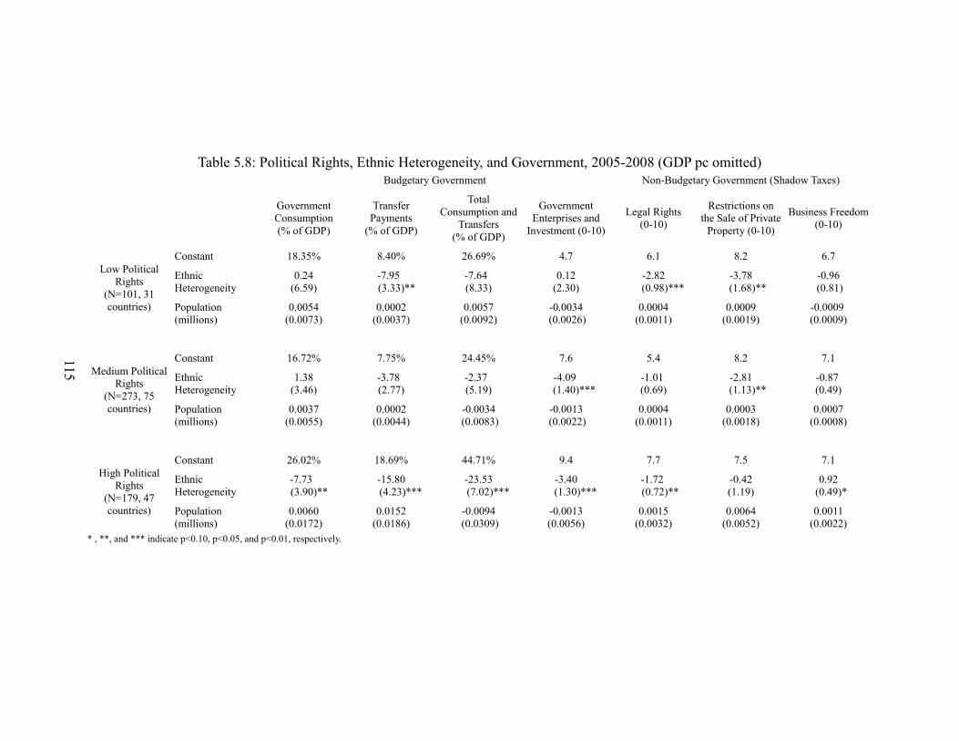
Table 5.8: Political Rights, Ethnic Heterogeneity, and Government, 2005-2008 (GDP pc omitted)Budgetary Government Non-Budgetary Government (Shadow Taxes)
Government Consumption(% of GDP)
Transfer Payments
(% of GDP)
Total Consumption and
Transfers(% of GDP)
Government Enterprises and
Investment (0-10)
Legal Rights(0-10)
Restrictions on the Sale of Private
Property (0-10)
Business Freedom(0-10)
Low Political Rights
(N=101, 31 countries)
Constant 18.35% 8.40% 26.69% 4.7 6.1 8.2 6.7
Ethnic Heterogeneity
0.24(6.59)
-7.95 (3.33)**
-7.64 (8.33)
0.12(2.30)
-2.82 (0.98)***
-3.78 (1.68)**
-0.96 (0.81)
Population(millions)
0.0054(0.0073)
0.0002(0.0037)
0.0057(0.0092)
-0.0034 (0.0026)
0.0004(0.0011)
0.0009(0.0019)
-0.0009 (0.0009)
Medium Political Rights
(N=273, 75 countries)
Constant 16.72% 7.75% 24.45% 7.6 5.4 8.2 7.1
Ethnic Heterogeneity
1.38(3.46)
-3.78 (2.77)
-2.37 (5.19)
-4.09 (1.40)***
-1.01 (0.69)
-2.81 (1.13)**
-0.87 (0.49)
Population(millions)
0.0037(0.0055)
0.0002(0.0044)
-0.0034 (0.0083)
-0.0013 (0.0022)
0.0004(0.0011)
0.0003(0.0018)
0.0007(0.0008)
High Political Rights
(N=179, 47 countries)
Constant 26.02% 18.69% 44.71% 9.4 7.7 7.5 7.1
Ethnic Heterogeneity
-7.73 (3.90)**
-15.80 (4.23)***
-23.53 (7.02)***
-3.40 (1.30)***
-1.72 (0.72)**
-0.42(1.19)
0.92 (0.49)*
Population(millions)
0.0060(0.0172)
0.0152(0.0186)
-0.0094 (0.0309)
-0.0013(0.0056)
0.0015(0.0032)
0.0064(0.0052)
0.0011(0.0022)
* , **, and *** indicate p<0.10, p<0.05, and p<0.01, respectively.
115

Table 5.9: Countries
Country Government Consumption
Transfer Payments
Total Gov't Share of GDP
Population(Millions)
Real GDP Per Capita,
2008 US $
Total Number of Observations
Albania 11.28% 6.85% 17.24% 3.1 $3,599.86 12
Algeria 25.83% 8.37% 32.80% 30.6 $5,786.63 12
Argentina 15.65% 9.03% 24.68% 36.9 $12,460.84 12
Australia 23.45% 11.99% 35.44% 19.4 $30,635.71 12
Austria 25.03% 26.25% 51.28% 8.1 $31,048.22 12
Bahamas 17.50% 3.68% 21.17% 0.3 $24,449.19 12
Bahrain 32.09% 3.40% 35.50% 0.7 $22,105.97 12
Bangladesh 6.05% 2.28% 7.75% 142.0 $1,944.11 12
Barbados 24.86% 4.80% 29.66% 0.3 $22,691.78 12
Belgium 26.77% 24.71% 51.48% 10.3 $29,169.77 12
Belize 17.38% 1.56% 18.94% 0.3 $8,095.72 10
Benin 13.79% 1.11% 14.45% 6.9 $1,364.84 12
Bolivia 16.74% 4.68% 21.42% 8.4 $3,397.99 12
Botswana 41.79% 9.13% 50.92% 1.7 $7,389.17 12
Brazil 23.91% 12.76% 36.67% 175.0 $8,672.19 12
Bulgaria 19.90% 16.89% 36.80% 8.0 $7,513.22 12
Burundi 18.24% 2.21% 20.45% 6.8 $760.08 12
Cameroon 13.07% 1.98% 15.05% 16.1 $2,690.67 12
Canada 26.15% 12.56% 38.70% 30.9 $31,253.94 12
Central Afr. Rep. 11.09% 0.00% 11.09% 3.8 $948.33 12
Chad 9.34% 0.67% 10.08% 8.8 $1,859.44 12
Chile 15.91% 11.06% 26.97% 15.4 $14,006.51 12
China 25.03% 6.82% 29.01% 1,250.0 $4,778.93 12
Colombia 21.51% 6.51% 28.02% 40.1 $6,797.42 12
Congo, Dem. R. 8.72% 0.65% 9.37% 52.5 $132.50 12
Congo, Rep. Of 28.70% 3.25% 31.44% 3.1 $3,793.24 12
Costa Rica 18.34% 5.20% 23.54% 4.0 $9,671.50 12
Cote d'Ivoire 13.82% 2.27% 15.71% 17.3 $2,577.80 12
Croatia 26.76% 20.24% 47.00% 4.5 $10,534.56 10
Cyprus 21.43% 12.44% 33.87% 0.8 $20,138.65 12
Czech Rep. 30.35% 27.87% 57.13% 10.3 $18,151.78 12
Denmark 34.69% 22.40% 57.09% 5.3 $29,683.18 12
Dominican Rep. 8.64% 4.13% 12.78% 8.9 $7,271.96 12
Ecuador 13.76% 1.73% 15.49% 12.2 $5,439.84 12
Egypt 14.12% 6.58% 20.70% 71.1 $4,667.85 12
El Salvador 10.17% 1.74% 11.91% 5.9 $5,061.63 12
Estonia 25.79% 13.42% 39.21% 1.4 $12,672.31 10
Fiji 23.85% 4.22% 28.07% 0.8 $5,429.55 10
Finland 29.40% 19.63% 49.03% 5.2 $26,829.02 12
France 29.09% 25.45% 54.54% 59.5 $26,860.10 12
Gabon 22.98% 1.33% 24.30% 1.2 $8,823.04 12
Germany 24.64% 26.08% 50.71% 81.7 $27,234.27 12
116
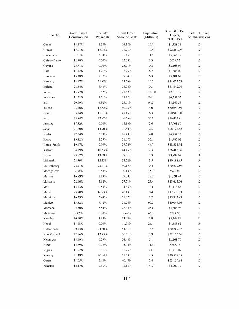
Country Government Consumption
Transfer Payments
Total Gov't Share of GDP
Population(Millions)
Real GDP Per Capita,
2008 US $
Total Number of Observations
Ghana 14.88% 1.50% 16.38% 19.8 $1,428.18 12
Greece 17.91% 18.34% 36.25% 10.9 $22,200.99 12
Guatemala 8.11% 3.34% 11.45% 11.5 $5,566.17 12
Guinea-Bissau 12.88% 0.00% 12.88% 1.3 $634.75 12
Guyana 25.71% 0.00% 25.71% 0.8 $2,263.99 12
Haiti 11.52% 1.21% 12.73% 8.7 $1,686.00 12
Honduras 15.38% 2.37% 17.74% 6.3 $3,301.61 12
Hungary 13.67% 21.88% 35.56% 10.2 $14,072.73 12
Iceland 28.54% 8.40% 36.94% 0.3 $31,842.76 12
India 15.97% 5.52% 21.49% 1,020.0 $2,815.15 12
Indonesia 11.71% 7.51% 19.22% 206.0 $4,257.52 12
Iran 20.69% 4.92% 25.61% 64.3 $8,247.55 12
Ireland 23.16% 17.82% 40.98% 4.0 $30,690.89 12
Israel 33.14% 15.01% 48.15% 6.3 $20,906.90 12
Italy 23.84% 22.82% 46.66% 57.8 $26,434.91 12
Jamaica 17.52% 0.98% 18.50% 2.6 $7,901.50 12
Japan 21.80% 14.70% 36.50% 126.0 $28,125.52 12
Jordan 22.54% 5.93% 28.48% 4.8 $4,954.15 12
Kenya 19.42% 2.25% 21.67% 32.1 $1,985.02 12
Korea, South 19.17% 9.09% 28.26% 46.7 $18,281.54 12
Kuwait 34.79% 10.53% 44.45% 2.3 $36,483.96 12
Latvia 23.62% 13.39% 37.01% 2.3 $9,887.67 10
Lithuania 22.39% 12.33% 34.72% 3.5 $10,198.65 10
Luxembourg 28.51% 22.61% 49.17% 0.4 $60,832.59 12
Madagascar 9.38% 0.88% 10.18% 15.7 $929.60 12
Malawi 16.89% 2.19% 19.09% 12.2 $1,091.43 12
Malaysia 22.10% 5.62% 27.71% 23.4 $13,655.06 12
Mali 14.13% 0.59% 14.66% 10.8 $1,113.68 12
Malta 23.90% 16.23% 40.13% 0.4 $17,530.33 12
Mauritius 16.39% 5.48% 21.87% 1.2 $15,312.43 12
Mexico 13.82% 7.42% 21.24% 97.3 $10,047.36 12
Morocco 22.50% 5.84% 28.34% 28.8 $4,866.92 12
Myanmar 8.42% 0.00% 8.42% 46.2 $214.50 12
Namibia 30.10% 3.34% 33.44% 1.9 $5,549.81 11
Nepal 11.08% 0.00% 11.08% 26.1 $1,688.62 10
Netherlands 30.13% 24.68% 54.81% 15.9 $30,267.97 12
New Zealand 22.86% 13.45% 36.31% 3.9 $22,125.66 12
Nicaragua 18.19% 6.29% 24.48% 5.1 $2,261.70 12
Niger 14.79% 0.79% 15.06% 11.5 $868.77 12
Nigeria 11.62% 0.11% 11.73% 128.0 $1,718.09 12
Norway 31.49% 20.04% 51.53% 4.5 $40,577.05 12
Oman 38.05% 2.40% 40.45% 2.4 $23,139.64 12
Pakistan 12.47% 2.66% 15.13% 141.0 $2,902.79 12
117

Country Government Consumption
Transfer Payments
Total Gov't Share of GDP
Population(Millions)
Real GDP Per Capita,
2008 US $
Total Number of Observations
Panama 19.23% 5.95% 25.18% 3.0 $7,281.20 12
Pap. New Guinea 21.59% 2.64% 24.17% 5.5 $2,142.01 12
Paraguay 12.01% 3.18% 15.18% 5.4 $4,763.64 12
Peru 12.59% 3.12% 15.71% 26.0 $5,301.55 12
Philippines 12.96% 2.40% 15.36% 78.5 $3,890.80 12
Poland 22.85% 20.98% 43.84% 38.1 $10,968.16 12
Portugal 23.44% 17.88% 41.32% 10.3 $18,008.36 12
Romania 14.87% 13.18% 28.05% 22.1 $3,265.83 12
Russia 25.18% 12.84% 38.02% 144.0 $9,669.73 10
Rwanda 11.95% 2.20% 14.15% 8.5 $987.05 10
Senegal 13.35% 2.70% 16.05% 10.1 $1,849.54 12
Sierra Leone 13.25% 2.04% 15.29% 4.6 $2,011.38 12
Singapore 20.49% 3.38% 23.86% 4.0 $32,728.01 12
Slovak Rep 25.61% 20.17% 43.72% 5.4 $12,691.25 10
Slovenia 26.51% 22.09% 48.60% 2.0 $19,834.21 10
South Africa 23.88% 5.20% 29.08% 43.7 $9,004.32 12
Spain 22.68% 16.01% 38.70% 41.8 $25,160.68 12
Sri Lanka 12.43% 5.03% 17.47% 18.8 $4,592.51 12
Sweden 35.49% 24.27% 59.75% 8.9 $27,774.18 12
Switzerland 16.82% 14.28% 31.10% 7.2 $34,513.85 12
Syria 17.23% 0.00% 17.23% 17.1 $2,491.44 12
Taiwan 18.44% 3.27% 21.71% 18.1 $20,194.72 12
Tanzania 17.38% 0.43% 17.82% 35.0 $753.57 12
Thailand 16.86% 2.48% 19.34% 62.9 $7,393.46 12
Togo 11.27% 2.13% 12.36% 5.4 $979.87 12
Trinidad & Tob. 19.66% 8.39% 28.05% 1.3 $16,985.83 12
Tunisia 20.13% 8.88% 29.01% 9.5 $7,831.60 12
Turkey 15.50% 5.56% 21.07% 66.7 $6,315.05 12
Uganda 14.11% 6.94% 21.05% 25.3 $1,038.86 12
Ukraine 25.56% 18.36% 42.01% 48.0 $7,018.26 10
Unit. Arab Em. 24.00% 1.48% 25.38% 3.4 $45,135.52 12
United Kingdom 24.54% 14.78% 39.32% 59.3 $27,118.53 12
United States 18.79% 12.83% 31.62% 283.0 $37,927.73 12
Uruguay 14.51% 14.94% 29.45% 3.3 $10,487.70 12
Venezuela 17.29% 11.25% 28.54% 24.5 $10,687.34 12
Zambia 16.75% 2.72% 19.47% 10.6 $1,450.29 12
Zimbabwe 27.12% 8.43% 35.55% 11.9 $3,484.93 12
118

Table 5.10: Summary Statistics, 1985-2008 (N=1436)
VariableMeans by Level of Political Rights
Low Political Rights Med Political Rights High Political Rights
Government Consumption(% of GDP) 18.52 17.61 23.72
Transfer Payments (% of GDP) 4.00 5.33 15.66
Total Government (% of GDP) 22.02 22.80 39.33
Government-Owned Enterprises 3.6 5.0 7.6
Legal and Property Rights 4.5 4.8 7.5
Freedom to Transfer Property 6.0 6.6 7.6
Business Freedom 5.4 6.1 6.9
Population (millions) 78.6 44.8 24.4
Real GDP Per Capita (2008 US$) $6,365.70 $6,656.05 $23,011.88
Ethnic Heterogeneity 0.54 0.52 0.27
Total Budgetary Government Legal and Property Rights
Legal and Property Rights 0.64***
Business Freedom 0.32*** 0.49***
VariableCorrelations with Ethnic Heterogeneity by Level of Political Rights
Low Political Rights Med Political Rights High Political Rights
Government Consumption(% of GDP) -0.19*** 0.02 -0.28***
Transfer Payments (% of GDP) -0.44*** -0.27*** -0.39***
Total Government (% of GDP) -0.33*** -0.12*** -0.40***
Legal and Property Rights -0.31*** -0.09** -0.27***
Business Freedom -0.08 -0.05 0.18***
Population (millions) -0.31*** -0.06 0.02
Real GDP Per Capita (2008 US$) -0.10* -0.20*** -0.16***
119

Table 5.11: Political Rights, Ethnic Heterogeneity, and Government, 1985-2008Budgetary Government Non-Budgetary Government
(Shadow Taxes)
Government Consumption(% of GDP)
Transfer Payments(% of GDP)
Total Consumption and Transfers
(% of GDP)
Legal Rights(0-10)
Business Freedom(0-10)
Low Political Rights
(N=268, 50 countries)
Constant 14.89% 14.26% 25.39% 5.4 4.6
Ethnic Heterogeneity
-1.21 (3.44)
-15.89 (3.28)***
-15.55 (4.81)***
-2.15 (0.84)***
0.74(0.75)
Population(millions)
0.0062(0.0044)
0.0018(0.0038)
0.0043 (0.0061)***
-0.0003 (0.0011)
0.0018 (0.0009)*
GDP Per Capita (thousands)
0.59 (0.09)***
0.04(0.06)
0.71 (0.12)***
0.06 (0.02)***
0.02(0.02)
Medium Political Rights
(N=671, 88 countries)
Constant 15.59% 11.94% 27.24% 4.8 5.6
Ethnic Heterogeneity
1.02(2.85)
-12.09 (2.57)***
-11.32 (4.50)***
-0.80(0.60)
0.33(0.42)
Population(millions)
0.0001(0.0047)
0.0025(0.0036)
0.0039(0.0066)
0.0013(0.0011)
0.0011(0.0008)
GDP Per Capita (thousands)
0.29 (0.06)***
0.056(0.042)
0.325 (0.078)***
0.052 (0.013)***
0.006(0.009)
High Political Rights
(N=497, 54 countries)
Constant 24.54% 17.98% 41.33% 6.0 6.7
Ethnic Heterogeneity
-8.19 (3.34)***
-15.82 (3.76)***
-25.15 (5.96)***
-1.34 (0.51)***
0.34(0.41)
Population(millions)
0.0099(0.0148)
0.0033(0.0167)
-0.0063 (0.0025)
-0.0031(0.0024)
0.0048 (0.0020)**
GDP Per Capita (thousands)
0.045(0.040)
0.046(0.046)
0.030(0.061)
0.082 (0.008)***
0.005(0.007)
120

Chapter 6: Discussion and Conclusions
This study explores different topics related to preferences for public provision by
heterogeneous groups. While the Tiebout mechanism may not produce a completely
efficient solution to the public goods problem, individual-level migration decisions may
still provide information about preferences for public provision. Chapter 3 tests this idea
using 2000 census migration data to explore the extent to which migration decisions can
be used to estimate demand for public provision of goods and services. Migration
patterns for various demographic groups are compared to relative changes in balanced-
budget fiscal policy outcomes taken from the census of governments.
In general, individuals are found to migrate in response to relative changes in
fiscal policies. However, the ability of provision to attract mobile individuals is limited
to expenditures on education, as individuals appear to be migrating away from increases
in other types of expenditures. Young individuals with relatively high levels of income
and/or education have more elastic migration responses to all types of fiscal policy. In
this analysis, each demographic subgroup is considered separately, and their underlying
level of mobility is captured in the estimated constant terms. Estimated differences
between each subgroup's migration responses in reaction to relative changes in fiscal
policy represent differences in preference intensity.
If, after controlling for their higher propensity to migrate, young college-educated
individuals are still more likely to move in response to relative changes in education
spending than individuals of retirement age, it must be the case that these young have a
higher preference intensity for education spending. While individuals of retirement age
121
may still feel strongly about education spending, they are less likely to consume publicly-
provided educational services. This contributes to the public finance literature by
providing a method to rank preference intensity for different types of public provision. A
detailed analysis using information at the local jurisdictional level would be able to
provide information on more fiscal categories.
One limitation of this study is that it does not control for tax progressivity at the
state level. A similar analysis using more detailed information on individual-level tax
burdens could be used to find the optimal levels of tax progressivity, and individual
demand for public provision could be matched to individual willingness-to-pay for
provision.
While preference intensity among groups can be ranked using this method, the
extent to which these policies can ultimately attract mobile individuals depends on the
underlying level of mobility. While migration outcomes are known, the overall level of
mobility in the population remains unclear, since satisfied mobile individuals who choose
not to move cannot be empirically separated from immobile, dissatisfied individuals.
Simulations provide upper and lower bound estimates of migration responses to
fiscal policy under the respective assumptions that the entire population, and only those
who actually migrated are mobile. Results indicate that an individual can be attracted to
a jurisdiction with an expenditure of somewhere between $479.11 and $6493.22 on
higher education.
One goal of this study was to create a revealed-preference method that can be
used to estimate demand for publicly provided goods and services. Quadratic
122

specifications are estimated in order to search for “bliss points.” If, for example, relative
changes in jurisdiction B are twice that of jurisdiction A, we might expect a greater
migration response with respect to jurisdiction B. Due to diminishing returns, this
migration response in jurisdiction B should be less than twice that in jurisdiction A, and
the estimated point where the migration response would be zero would be considered the
bliss point.
However, diminishing returns to relative changes do not regularly appear in the
aggregate fiscal data. This may be due to aggregation bias or policy convergence and
low levels of variation among jurisdictions. Individuals may be less aware of relatively
small fiscal changes, and there may initially be an increasing response to fiscal changes.
Because extreme fiscal changes do not appear in the data, we do not observe the
diminishing responses. Because of this, the quadratic specifications estimated in Table
3.7 are not concave with respect to the origin, and maxima (i.e., bliss points) cannot be
found.
This also provides insight into the race-to-the-bottom literature. Low-income
individuals are found to actually migrate away from balanced-budget increases in welfare
spending, inconsistent with welfare migration. Also inconsistent with the theory, college-
educated and high-income individuals do not appear more averse to welfare spending
than other groups. Brueckner (2000) finds that states most likely are competing with one
another in a race to lower welfare benefits, but in the absence of welfare migration these
actions would require additional justification. In addition, if welfare migration is not
widespread, then federal programs (e.g., matching grants) intended to address this
123

phenomenon would be counterproductive. This study shows that all individuals appear to
demand less provision of welfare, and that a reduction in provision reflects the underlying
preferences of the entire population.
Both the race-to-the-bottom literature and the Tiebout hypothesis suggest that
policies have the ability to change the demographic makeup within a jurisdiction.
Though certain fiscal policies may be more attractive to some individuals, the ability of
policy to have an affect on the population is limited in the short-run because fiscal
policies will attract individuals from many different demographic groups. Because of the
pre-existing level of demographic heterogeneity in the overall economy, some level of
demographic heterogeneity will remain within each jurisdiction.
Chapter 5 explores the relationship between heterogeneity and the size of
government, while considering the possibility that non-budgetary intervention through
regulation can also exist in addition to fiscal policy. Because there is relatively little
variation in heterogeneity in the U.S., this chapter explores this idea in an international
context. In general, heterogeneous countries are found to have lower levels of transfer
payments, consistent with predictions in the literature.
Additionally, the relationships between heterogeneity and government size are
found to be dependent upon the level of political rights in a country. In countries with
high levels of political rights, heterogeneous jurisdictions are found to have lower levels
of budgetary government consumption. In countries with low levels of political rights,
heterogeneity does not appear to have an effect on government consumption.
The effect of heterogeneity on non-budgetary government is unclear in
124

democracies. Heterogeneity is found to increase the size of non-budgetary government in
non-democratic countries. Also, the effect of heterogeneity on non-budgetary
government appears to be larger in countries with low levels of property rights. If
transfer payments are excluded, heterogeneity increases the overall size of government in
non-democratic countries.
A future study will explore the relationships between fiscal policy and
centralization in a federal system while explicitly controlling for this demographic
heterogeneity. If more centralized jurisdictions are larger than decentralized jurisdictions,
they are likely to have more heterogeneous populations. If these heterogeneity affects
preferences for public provision, then previous tests of the “Leviathan” theory that do not
consider heterogeneity may be biased. The inclusion of non-budgetary government
activity in such a study may yield insightful results.
In addition, previous research has found evidence of “Wagner's Law” in
industrialized nations, but little evidence in developing countries (Akitoby et al, 2006).
Future research will examine the extent to which these non-budgetary measures can be
used to explain this difference.
125

References
Aaron, H. J. “Local public expenditures and the 'migration effect'." Economic Inquiry 7, no. 4 (2007): 385–390.
Acemoglu, D., J. A Robinson, and T. Verdier. “Kleptocracy and divide-and-rule: a model of personal rule.” Journal of the European Economic Association 2, no. 2 (2004): 162–192.
Akitoby, B., B. Clements, S. Gupta, and G. Inchauste. “Public spending, voracity, and Wagner's law in developing countries.” European Journal of Political Economy 22, no. 4 (2006): 908–924.
Alesina, A., and E. Spolaore. 2005. The size of nations. The MIT Press.
Anderson, L. R, J. M Mellor, and J. Milyo. “An Experimental Study of the Effects of Inequality and Relative Deprivation on Trusting Behavior.” Working Paper (2005).
Anderson, L. R, J. M Mellor, and J. Milyo. “Induced heterogeneity in trust experiments.” Experimental Economics 9, no. 3 (2006): 223–235.
Anderson, Robert and Crocker, Thomas. "Air Pollution and Residential Property Values." Urban Studies, 8 (October 1971): 171-80.
Anderson, Soren and Richard G. Newell. “Simplified marginal effects in discrete choice models.” Economics Letters, 81 (2003): 321-326.
Annett, A. 2001. Social fractionalization, political instability, and the size of government. IMF Staff Papers: 561–592.
Barone, Enrico, 1912a, Studi di economia finanziaria, in Giornale degli economisti, in R. Musgrave & A.T. Peacock, eds.,Classics in the Theory of Public Finance. London-New York: Macmillan, 1958, pp.165-67.
Barzel, Yoram. “Two Propositions on the Optimum Level of Producing Collective Goods,” Public Choice 6 (Spring 1969): 31-37.
Barzel, Yoram. “Private Schools and Public School Finance.” The Journal of Political Economy, Vol. 81, No. 1 (Jan.-Feb., 1973): pp. 174-186.
Bastable, C. F. 1892. Public finance. London-New York: Macmillan and Co.
126

Bergstrom, Theodore C., Judith A. Roberts, Daniel L. Rubinfeld, and Perry Shapiro. “A test for efficiency in the supply of public education.” Journal of Public Economics 35, no. 3 (1988): 289–307.
Besley, Timothy, and Anne C. Case, "Does Electoral Accountability Affect Economic Policy Choices? Evidence from Gubernatorial Term Limits.” Quarterly Journal of Economics, Vol. 110, No. 3, (Aug., 1995): pp. 769-798
Besley, Timothy, and Anne C. Case, "Incumbent Behavior: Vote Seeking Tax Setting and Yardstick Competition," American Economic Review, LXXXV (1995): 25-45.
Besley, Timothy and Michael Smart. “Does tax competition raise voter welfare?” CEPR discussion paper 3131, 2002.
Black, Dan A., and William H. Hoyt. “Bidding for Firms.” The American Economic Review 79, no. 5 (December 1989): 1249-1256.
Boettke, Peter. 2001. Calculation and Coordination: Essays on Socialism and Transitional Political Economy. London: Routledge.
Breeden, Charles H., and William J. Hunter. “Tax Revenue and Tax Structure.” Public Finance Review 13, no. 2 (April 1, 1985): 216-224.
Brennan, Geoffrey. “Public finance, public choice and the political economy of regulation.” in Winer, S. L, and H. Shibata., ed., Political economy and public finance: the role of political economy in the theory and practice of public economics. Edward Elgar Pub.2002. 13-30.
Brennan, G., and Buchanan, J.M. (1980) The Power to Tax: Analytical Foundations of a Fiscal Constitution. Cambridge: Cambridge University Press.
Brookshire, David S., Mark A. Thayer, William D. Schulze, and Ralph C. d'Arge. “Valuing Public Goods: A Comparison of Survey and Hedonic Approaches.” The American Economic Review 72, no. 1 (March 1982): 165-177.
Brueckner, Jan K. “A Test for Allocative Efficiency in the Local Public Sector.” Journal of Public Economics 19 (1982): 311-331.
Brueckner Jan K. “Welfare Reform and the Race to the Bottom: Theory and Evidence.” Southern Economic Journal, Vol. 66, No. 3. (Jan., 2000), pp. 505-525.
Brueckner, J. K., and L. A. Saavedra. “Do local governments engage in strategic tax competition?” National Tax Journal 54 (2001): 203-29.
127

Buchanan, James M “Federalism and Individual Sovereignty.” Cato Journal v15 (1995): 2-3.
Buchanan, James M and Richard A Musgrave (1999). Public Finance and Public Choice: Two Contrasting Visions of the State. MIT
Bullock, Charles J. (1906) Selected Readings in Public Finance, Boston, Ginn.
Campbell, Colin D., “New Hampshire's Tax-Base Limits: An Example of the Leviathan Model,” Public Choice 78, (February 1994): 129-44.
Caplan, B. “Mises’ democracy–dictatorship equivalence theorem: A critique.” The Review of Austrian Economics 21, no. 1 (2008): 45–59.
Carroll, Robert and Michael Wasylenko. “Do State Business Climates Still Matter? Evidence of a Structural Change.” National Tax Journal 47 No. 1 (March, 1994): 19-37.
Carson, R. T, N. E Flores, K. M Martin, and J. L Wright. “Contingent valuation and revealed preference methodologies: comparing the estimates for quasi-public goods.” Land Economics (1996): 80–99.
Case, A.C., H.S. Rosen and J.R. Hines, “Budget spillovers and fiscal policy interdependence: Evidence from the states” Journal of Public Economics 52 (1993): 285-307.
Cebula, Richard J. (2003) Net interstate population growth rates and the Tiebout-Tullock hypothesis: New empirical evidence, 1990–2000. Atlantic Economic Journal 30:4, 414-421
Cebula, Richard J. “An Empirical Note on the Tiebout-Tullock Hypothesis.” The Quarterly Journal of Economics, Vol. 92, No. 4, (Nov., 1978), pp. 705-711
Cebula, Richard J. “Interstate Migration and the Tiebout Hypothesis: A Disaggregated Analysis,.” Journal of the American Statistical Association, 69, 1974, pp. 876-9.
Cebula, R. J., Kohn, R. M. and Vedder, R. K. "Some Determinants of Interstate Migration of Blacks, 1965-1970," Western Econ. J;, Dec. 1973, 11(4), pp. 500-505.
Chandra, Amitabh and Eric Thompson, “Does public infrastructure affect economic activity? Evidence from the rural interstate highway system.” Regional Science and Urban Economics 30 (2000) 457–490
Charney, A. H. “Migration and the public sector: a survey.” Regional Studies 27, no. 4 (1993): 313–326.
128

Ciriacy-Wantrup, S. V. “Capital Returns from Soil-Conservation Practices.” Journal of Farm Economics 29, no. 4 (November 1947): 1181-1196.
Clark, D.E. and W.J. Hunter. 1992. “The Impact of Economic Opportunity, Amenities and Fiscal Factors in Age-Specific Migration Rates,” Journal of Regional Science, 32(3) (August): 349-365.
Clark, David E., Thomas A. Knapp, and Nancy E. White. “Personal and Location-Specific Characteristics and Elderly Interstate Migration.” Growth and Change 27, no. 3 (1996): 327-351.
Clawson, Marion. 1959. Methods of Measuring the Demand for and Value of Outdoor Recreation, Reprint No. 10 (Washington, D. C.: Resources for the Future), February.
Cohen, M. A, R. T. Rust, S. Steen, and S. T. Tidd. “Willingness-to-pay for crime control programs.” Criminology 42 (2004): 89.
Conway, Karen Smith and Andrew J Houtenville, “Elderly Migration and State Fiscal Policy: Evidence from the 1990 Census Migration Flows.” National Tax Journal 54 (1), March 2001, 103-124.
Conway, K. S.; Houtenville, A. J. .Do the Elderly Vote with Their Feet?,. Public Choice, 97, 1998, pp. 663-85.
Conway, Karen Smith, and Jonathan C. Rork. “Diagnosis Murder: The Death of State ‘Death’ Taxes.” Economic Inquiry 42 No. 4 (October, 2004): 537–59.
Conway, K.S., Rork, J.C., 2006. State death taxes and elderly migration—The chicken or the egg? National Tax Journal 59 (1), 97–128.
Coomes, Paul A. and William H Hoyt, “Income taxes and the destination of movers in multistate MSAs.” Journal of Urban Economics, 2008, 920-937.
Costa, D. L. & Kahn, M. E. 2003a. “Cowards and Heroes: Group Loyalty in the American Civil War,” Quarterly Journal of Economics 118, 519–48.
Costa, D. L. and Kahn, M. E. (2003b), ‘Civic Engagement and Community Heterogeneity, An Economist’s Perspective’,Perspectives on Politics, 1, 103–11.
Coughlin, C. C, T. A Garrett, and R. Hernández-Murillo. “Spatial dependence in models of state fiscal policy convergence” Working Paper, St Louis Federal Reserve, (2006).
129

Cushing, Brian J. “The Effect of the Social Welfare System on Metropolitan Migration in the US, by Income Group, Gender and Family Structure.” Urban Studies 1993 30: 325-337
Cutler, D. M., D. W. Elmendorf, and R. J. Zeckhauser 1993. “Demographic Characteristics and the Public Bundle,” Public Finance/Finances Publiques, 48, 178–198.
Dahl, Robert Alan, and Edward R. Tufte. Size and Democracy. Stanford University Press, 1973.
Davis, R. K. “Recreation planning as an economic problem.” Nat. Resources J. 3 (1963): 239.
Deacon, Robert T. 1979. “The Expenditure Effects of Alternative Public Supply Institutions.” Public Choice 34, no. 3/4: 381-397.
De Viti de Marco, A. 1888. Il carattere teorico dell’economia finanziaria. Roma, Pasqualucci. Engl. translation of the first chapter: The “Theory” and “Application” of Economic Doctrines, Rivista di politica economica 37, no. 6-7: 277–303.
Dewenter, Kathryn L. and Paul H. Malatesta “State-Owned and Privately Owned Firms: An Empirical Analysis of Profitability, Leverage, and Labor Intensity.” The American Economic Review, Vol. 91, No. 1 (Mar., 2001), pp. 320-334
Diamond, J. “Wagner's "Law" and the Developing Countries.” The Developing Economies 15, no. 1, March 1977: 37–59.
DiLorenzo, Thomas J. 1983. “Economic Competition and Political Competition: An Empirical Note.” Public Choice 40, no. 2: 203-209.
Dowding, Keith, Peter John and Stephen Biggs, “Tiebout: A Survey of the Empirical Literature.” Urban Studies 1994; 31; 767
Dreher, A., P. G Méon, and F. Schneider. “The devil is in the shadow: do institutions affect income and productivity or only official income and official productivity?” CESifo Working Paper No. 2150, 2007.
Eberts, Randall W. and Timothy J. Gronberg (1990), “Structure, Conduct, and Performance in the Local Public Sector,” National Tax Journal 43(2), pp. 165-174.
Ehdaie, J. 1994. “Fiscal decentralization and the size of the government: an extension with evidence from cross-country data.” World Bank, Policy Research Working Paper Series.
130

Epple, Dennis and Richard E. Romano. “Ends against the middle: Determining public service provision when there are private alternatives.” Journal of Public Economics 62 (1996), 297-325.
Eris, Mehmet. “Population heterogeneity and growth.” Economic Modelling In Press, (2010).
Fiva, Jon (2006). “New Evidence on the Effect of Fiscal Decentralization on the Size and Composition of Government Spending.” Public Finance Analysis 62 (2): 250-80.
Forbes, Kevin F. and Ernest M. Zampelli, “Is Leviathan a Mythical Beast?” The American Economic Review, Vol. 79, No. 3 (Jun., 1989), pp. 568-577
Fossati, Amedeo. “Needs, the Principle of Minimum Means, and Public Goods in De Viti de Marco.” Journal of the History of Economic Thought, Forthcoming. Available at SSRN: http://ssrn.com/abstract=799684
Gabriel, Stuart A., Joe P. Mattey, and William L. Wascher, “Compensating differentials and evolution in the quality-of-life among U.S. states.” Regional Science and Urban Economics 33 (2003) 619-649.
Gale, L. R.; Heath, W. C. .Elderly Internal Migration in the United States Revisited,. Public Finance Review, 28, March, 2000, pp. 153-70.
Gallego, M., and C. Pitchik. “An economic theory of leadership turnover.” Journal of Public Economics 88, no. 12 (2004): 2361–2382.
Ghatak, S., P. Levine, and S. W Price. “Migration theories and evidence: an assessment.” Journal of Economic Surveys 10, no. 2 (1996): 159–198.
Giertz, J. Fred, “Centralization and Government Budget Size.” Publius v11,1 (1981).
Glaeser, Edward, Gyourko, Joseph and Raven Saks (2006) “Urban Growth and HousingSupply,” Journal of Economic Geography 6(1): 71-89.
Glaeser, E. L, and R. E Saks. 2006. “Corruption in America.” Journal of Public Economics 90, no. 6-7: 1053–1072.
Glaeser, Edward L. and Kristina Tobio, “The Rise of the Sunbelt.” HIER Discussion Paper 2135, April 2007.
Glaeser, E. L. et al. 2000. ‘Measuring Trust’, Quarterly Journal of Economics 115, 811–46.
131
Goldin, Claudia and Lawrence F. Katz. 1999. “Human Capital and Social Capital: The Rise of Secondary Schooling in America, 1910 to 1940.” Journal of Interdiscimplinary History. 29: 683-723.
Goldstein, G. S, and M. V Pauly. “Tiebout bias on the demand for local public goods.” Journal of Public Economics 16, no. 2 (1981): 131–143.
Graves, P.E. and P. Linneman. 1979. “Household Migration: Theoretical and Empirical Results.” Journal of Urban Economics, no 6, 383-404.
Greenwood, Michael. “Research on Internal Migration in the U.S.: A Survey.” Journal of Economic Literature 13 (June 1975): 397-433.
Greenwood, Michael. “Human Migration: Theory, Models, and Empirical Studies.” Journal of Regional Science, Vol. 25, No. 4, 1985.
Greenwood, M. J. “Migration: a review.” Regional Studies 27, no. 4 (1993): 295–296.
Greenwood, Michael J., Peter R. Mueser, David A. Plane, and Alan M. Schlottmann. “New directions in migration research.” The Annals of Regional Science 25, no. 4 (December 1, 1991): 237-270.
Grossman, Philip J., and Edwin G. West. 1994. “Federalism and the Growth of Government Revisited.” Public Choice 79, no. 1/2: 19-32.
Gupta, S., L. Leruth, L. De Mello, and S. Chakravarti. 2003. “Transition Economies: How appropriate is the size and scope of Government?” Comparative Economic Studies 45, no. 4: 554–577.
Habyarimana, James P., Macartan Humphreys, Daniel N. Posner, and Jeremy M. Weinstein, 2007. “Why Does Ethnic Diversity Undermine Public Goods Provision? An Experimental Approach.” American Political Science Review, Vol. 101, No. 4
Habyarimana, James, Macartan Humphreys, Daniel N. Posner & JeremyWeinstein. 2009. Coethnicity: Diversity and the Dilemmas of Collective Action. New York: Russell Sage Foundation.
Hall, Joshua C., and Peter T. Leeson. “Racial Fractionalization and School Performance.” American Journal of Economics and Sociology 69, no. 2 (4, 2010): 736-758.
Hansen, T. B. “The willingness-to-pay for the Royal Theatre in Copenhagen as a public good.” Journal of Cultural Economics 21, no. 1 (1997): 1–28.
132
Harden, J. William and William H. Hoyt. “Do States Choose Their Mix of Taxes to Minimize Employment Losses?” National Tax Journal 56, No. 1 (March, 2003): 7-26.
Harrison, David, and Daniel Rubinfeld. “Hedonic housing prices and the demand for clean air.” Journal of Environmental Economics and Management 5, no. 1 (1978): 81–102.
Hayek, F.A. 1939. ‘The Economic Conditions of Interstate Federalism.’ in Individualism and Economic Order. Chicago: University of Chicago Press, 255-272.
Helms, L. Jay, “The Effect of State and Local Taxes on Economic Growth: A Time Series-Cross Section Approach,” The Review of Economics and Statistics, 1985, pp. 574-582.
Hensher, D. A, and C. Sullivan. “Willingness to pay for road curviness and road type.” Transportation Research Part D: Transport and Environment 8, no. 2 (2003): 139–155.
Hirschman, Albert O,. Exit, Voice, and Loyalty: Responses to Decline in Firms, Organizations, and States. Cambridge, MA: Harvard University Press. 1970
Hirschman, Albert O. “Exit, Voice and the State.” World Politics, Vol. 31, No. 1 (Oct. 1978), 90-107.
Holtz-Eakin, Douglas, “Public-Sector Capital and the Productivity Puzzle.” The Review of Economics and Statistics, Vol. 76, No. 1 (Feb., 1994), pp. 12-21
Hotelling, H. 1949. Letter to National Park Service dated 1947 in An Economic Study of the Monetary Evaluation of Recreation in the National Parks. National Park Service and Recreational Planning Division, U.S. Department of the Interior, Washington, D.C.
Hoyt,W.H., 1991. “Property taxation, Nash equilibrium, and market power.” Journal of Urban Economics 30, 123–131.
Hoyt,W.H., 1992. “Market power of large cities and policy differences in metropolitan areas.” Regional Science and Urban Economics 22, 539–558.
Hoyt, W.H., 1993. “Tax competition, Nash equilibria, and residential mobility.” Journal of Urban Economics 34, 358–379
Hoyt,W.H., 1995. “Leviathan and local tax policies: do local governments maximize revenue.” Working Paper E-185-95, Center for Business and Economic Research, University of Kentucky.
133

Jacobs, L. R, and R. Y Shapiro. Politicians don't pander: Political manipulation and the loss of democratic responsiveness. University of Chicago Press, 2000.
Jin, Jing, and Heng-fu Zou. 2002. “How does fiscal decentralization affect aggregate, national, and subnational government size?” Journal of Urban Economics 52, no. 2 (September): 270-293.
Johnson, S., D. Kaufmann, A. Shleifer, M. I Goldman, and M. L Weitzman. “The unofficial economy in transition.” Brookings Papers on Economic Activity 1997, no. 2 (1997): 159–239.
Kahneman, D. and J. L. Knetsch, “Valuing public goods: The purchase of moral satisfaction” J. Environ. Econom. Manage., 22, 57-70 (1992).
Kaplan, Greg and Sam Schulhofer-Wohl. “Interstate Migration Has Fallen Less Than You Think: Consequences of Hot Deck Imputation in the Current Population Survey” Working Paper, Federal Reserve Bank of Minneapolis, Nov 2010.
Kau, J. B, and C. F. Sirmans. “New, repeat, and return migration: a study of migrant types.” Southern Economic Journal 43, no. 2 (1976): 1144–1148.
Kimenyi, M. S. “Ethnicity, governance and the provision of public goods.” Journal of African Economies 15, no. 1 (2006): 62.
Knack, S., and P. Keefer. “Does Social Capital Have An Economic Payoff? A Cross-Country Investigation.” Quarterly Journal of Economics 112, no. 4 (1997): 1251–1288.
Kneebone, Ronald D. 1992. Centralization and the size of government in Canada. Applied Economics 24, no. 12 (December): 1293.
La Porta R., F. Lopez de Silanes, A. Shleifer and R. Vishny (1999), “The Quality of Government”, Journal of Law, Economics and Organization, vol. 15, no. 1, March, pp. 222-279.
Laffer, Arthur and Stephen Moore (2007, December 10). The (Tax) War Between the States. Wall Street Journal (Eastern Edition), p.A.19.
Lee, K. “Tax Competition with Imperfectly Mobile Capital” Journal of Urban Economics 42, no. 2 (1997): 222–242.
Leeson, Peter T. “Balkanization and Assimilation: Examining the Effects of State-Created Homogeneity.” Review of Social Economy 65(2) 2007: 141-164.
134

Leigh, A. 2006a. “Trust, inequality and ethnic heterogeneity.” Economic Record 82, no. 258: 268–280.
Leigh, A. 2006b. “Does equality lead to fraternity?.” Economics letters 93, no. 1: 121–125.
Levitt, Steven, "The Effect of Prison Population Size on Crime Rates: Evidence from Prison Overcrowding Litigation." Quarterly Journal of Economics, 1996, 111(2), pp. 319-51.
Lindahl Erik. (1919): Die Gerechtigkeit der Besteuring, Lund: Gleerup. English translation: Just taxation-a positive solution. In Richard Musgrave and Alan Peacock, editors, Classics in the Theory of Public Finance, pages 98–123. Macmillan, London, 1958.
Llanto, G. 2009. Fiscal decentralization and local finance reforms in the Philippines. Discussion Papers. Phillippine Institute for Development Studies
Lowery, David, W. E. Lyons and Ruth Hoogland DeHoog, “The Empirical Evidence for Citizen Information and a Local Market for Public Goods.” The American Political Science Review, Vol. 89, No. 3 (Sep., 1995), pp. 705-707
Luttmer, E. F.P. “Group loyalty and the taste for redistribution.” Journal of Political Economy 109, no. 3 (2001).
Lyall, Jason. 2010 “Are Co-Ethnics More Effective Counter-Insurgents? Evidence from the Second Chechen War” American Political Science Review, 104:1 (February 2010), 1-20.
Mackenzie, G. A, and P. Stella. 1996. Quasi-fiscal operations of public financial institutions. Intl Monetary Fund.
Mauro, Paulo. “Corruption and growth.” The Quarterly Journal of Economics 110, no. 3 (1995): 681–712.
“Merkel erklärt Multikulti für gescheitert.” Spiegel Online [16 October 2010]. Available from: http://www.spiegel.de/politik/deutschland/0,1518,723532,00.html
Mincer, J. “Family migration decisions.” The Journal of Political Economy 86, no. 5 (1978): 749–773.
Mises, Ludwig von. 1957. Theory and History. New Haven, Connecticut: Yale University Press.
135

Misiolek, Walter S. and Harold W. Elder. “Tax Structure and the Size of Government: An Empirical Analysis of the Fiscal Illusion and Fiscal Stress Arguments” Public Choice, Vol. 57, No. 3 (1988), pp. 233-245
Mitchell, Robert Cameron and Richard T. Carson. Using surveys to value public goods: the contingent valuation method. Washington D.C., 1989, Resources for the Future
Mosca, Manuela. “De Viti de Marco, Historian of Economic Thought” (November 2002). Universita di Lecce Economics Working Paper No. 31/13. Available at SSRN: http://ssrn.com/abstract=448400 or doi:10.2139/ssrn.448400
Muth, Richard F. "Differential Growth Among Large U.S. Cities," in Papers in Quantitative Economics, edited by James P. Quirk and Arvid M. Zarley, Lawrence: The University Press of Kansas, 1968.
Muth, Richard F. “Migration: Chicken or Egg?.” Southern Economic Journal 37, no. 3 (January 1971): 295-306.
Myers, B. R. The cleanest race: how North Koreans see themselves--and why it matters. Melville House Publishing, 2010.
Nash, Fay F. “ESCAP II: Analysis of Census Imputations.” U.S. Census Bureau, Executive Steering Committee for ACE Policy II. Report Number 21, Sept 24, 2001
Nelson, Michael A., “Searching for Leviathan: Comment and Extension .” The American Economic Review, Vol. 77, No. 1, (Mar., 1987), pp. 198-204
Niskanen, William (1971). Bureaucracy and Representative Government. Chicago: Aldine, Atherton.
Niskanen, William, “The Peculiar Economics of Bureaucracy.” The American Economic Review, Vol 58, No 2, (May, 1968), pp. 293-305.
Niskanen, William (1992). “The Case for a New Fiscal Constitution.” Journal of Economic Perspectives, 6(2):13-24.
Oates, Wallace E. and John Wallis, “Decentralization in the Public Sector: An Empirical Study of State and Local Government," in H. Rosen, ed., Fiscal Federalism: Quantitative Studies (Chicago: University of Chicago Press, 1988), pp. 5-28.
Oates, Wallace E., “Searching for Leviathan: An Empirical Study” The American Economic Review, Vol. 75, No. 4, (Sep., 1985), pp. 748-757
136

Oates, W.E. (1969) “The effect of property taxes and local public spending on property values: an empirical study of tax capitalization and the Tiebout hypothesis,” Journal of Political Economy, 77, pp. 957-971.
Olson, Mancur, The Logic of Collective Action: Public Goods and the Theory of Groups, 1965, Harvard University Press.
Oxley, L. “Cointegration, causality and Wagner's Law: A test for Britain 1870-1913.” Scottish Journal of Political Economy 41, no. 3 (1994): 286.
Page, Scott E. The Difference: How the Power of Diversity Creates Better Groups, Firms, Schools, and Societies. 1st ed. Princeton University Press, 2008.
Poterba, J. M. 1997. “Demographic Structure and the Political Economy of Public Education”, Journal of Policy Analysis and Management 16, 48–66.
Putnam, R. D. “E Pluribus Unum: Diversity and community in the twenty-first century the 2006 Johan Skytte prize lecture.” Scandinavian Political Studies 30, no. 2 (2007): 137–174.
Puviani, Amilcare. 1896 “Il problema edonistico nella scienza delle finanze.” La Riforma Sociale, rassegna di scienza sociale e politiche. Anno III, Vol 6, pp. 297-309.
Ravenstein, E. G. The birthplaces of the people and the laws of migration. Trübner & Co., 1876. reprinted from The Geographical Magazine III, 173, 201, and 229 (1876).
Ravenstein, E. G. “The laws of migration.” Journal of the Statistical Society of London 48, no. 2 (1885): 167–235.
Ravenstein, E. G. “The laws of migration: second paper.” Journal of the Royal Statistical Society 52, no. 2 (1889): 241–305.
Rhode, Paul W. and Koleman S. Strumpf. “Assessing the Importance of Tiebout Sorting: Local Heterogeneity from 1850 to 1990.” American Economic Review, v 93, 5, 2003.
Rubinfield, D. L, P. Shapiro, and J. Roberts. “Tiebout bias and the demand for local public schooling.” The Review of Economics and Statistics 69, no. 3 (1987): 426–437.
Sachs, Natan B. 2009 “Experimenting with Identity: Islam, Nationalism and Ethnicity” Working Paper, Stanford University.
Sax, E. (1884), Das Wesen und die Aufgaben der Nationalökonomie, Vienna, Hölder.
Sax, E. (1887), Grundlegung der Theoretischen Staatswirthschaft, Vienna, Hölder.
137

Schneider, F., and D. Enste. Shadow economies around the world: size, causes, and consequences. International Monetary Fund, 2000.
Schuck, Peter H. Diversity in America: Keeping Government at a Safe Distance. Belknap Press of Harvard University Press, 2006.
Schwartz, A "Interpreting the Effect of Distance on Migration," Journal of Political Economy, Sept. / Oct., 1973, 81(5), pp. 1153-69.
Scully, Gerald W. “The Convergence of Fiscal Regimes and the Decline of the Tiebout Effect.” Public Choice, Vol 72. No 1 (Oct., 1991), pp. 51-59.
Shtatland, Ernest S., Sara Moore, and Mary B. Barton. “Why We Need an R2 Measure of Fit (and not only one) in Proc Logistic and Proc Genmod.” SUGI Proceeding 256-25, Sas Institute, 2000.
Sharp, Elaine B. “"Exit, Voice, and Loyalty" in the Context of Local Government Problems.” The Western Political Quarterly, Vol. 37, No. 1 (Mar., 1984), pp. 67-83
Shonchoy, A. 2010. “Determinants of Government Expenditure in Developing Countries-A Panel Data Approach” BRAC University Journal
Smith, V. K, and Y. Kaoru. 1990. “What have we learned since hotelling's letter?: A meta-analysis.” Economics Letters 32, no. 3: 267–272.
Sorens, Jason. “Fiscal Federalism: A Return to Theory and Measurement” (November 13, 2008). Available at SSRN: http://ssrn.com/abstract=1301096
Sorens, Jason. “The Politics and Economics of Official Ethnic Discrimination: A Global StatisticalAnalysis, 1950–2003.” International Studies Quarterly (2010) 54, 535–560
States of Opportunity. (2008, February 12). Wall Street Journal (Eastern Edition), p.A.16.
Stegarescu, D. (2005), Public Sector Decentralisation: Measurement Concepts and Recent International Trends.” Fiscal Studies, 301–333.
Steyn, Mark. “One-Man Stan..” Atlantic Monthly, March 2007.
Stigler, George J. “Economic Competition and Political Competition.” Public Choice 13 (September 1972): 91-106.
138

Stonecash, Jeffrey M. “Fiscal Centralization in the American States: Findings From Another Perspective.” Public Budgeting & Finance; Winter88, Vol. 8 Issue 4, pp. 81-89
Sugahara, K. 2009. “The Impact of Decentralization on Fiscal Competition: Evidence from Sub- National Governments in Japan.” Working Paper, Kyoto Sangyo University.
Stigler, G.J., 1957. '"Tenable Range of Functions of Local Government," in Joint Economic Committee, Subcommittee on Fiscal Policy, Federal Expenditure Policy for Economic Growth and Stability (Washington, DC, 1957), 213-19.
Tanzi, Vito, Fundamental Determinants of Inequality and the Role of Government (December 1998). IMF Working Paper, Vol. , pp. 1-24, 1998.
Tanzi, V., and L. Schuknecht. 2000. Public spending in the 20th century: A global perspective. Cambridge Univ Press.
Tax Foundation, Inc., Facts and Figures on Government Finance, 38th ed.,(Washington D.C.: Tax Foundation, Inc., 2005), Table D1, pp. 143-144
Teske, Paul Mark Schneider, Michael Mintrom, and Sam Best, “The Empirical Evidence for Citizen Information and A Local Market for Public Goods.” American Political Science Review, 89,1995: 707-709.
Todaro, Michael P. “A Model of Labor Migration and Urban Unemployment in Less Developed Countries.” The American Economic Review, Vol. 59, No. 1 (1969), pp. 138-148
Trice, Andrew H. and Samuel E. Wood. 1958. "Measurement of Recreation Benefits," Lands Economics 34 (February): 195-207.
Tullock, G. (1971) Public decisions as public goods, Journal of Political Economy, 79, pp. 913-919.
Tullock, G. “Social Cost and Government Action.” American Economic Review, Vol 59, No. 2, May 1969.
Umpfenbach, Karl. 1859. Lehrbuch der Finanzwissenschaft. Erlangen, Ferdinand Enke.
U.S. Census Bureau. Geographical Mobility, P20-497, P20-510, P20-520, P20-531, and P20-538. 1997-2001.
Vigdor, J. L. “Community composition and collective action: Analyzing initial mail response to the 2000 census.” Review of Economics and Statistics 86, no. 1 (2004): 303–312.
139

Wagner, Adolph. 1863. Die Ordnung des österreichischen Staathaushaltes, mit besonderer Rücksicht auf den Ausgabe-Etat und die Staatsschuld. Vienna, Carl Gerold.
Wagner, Adolph. Grundlegung der politischen Ökonomie, Bk. VI, ch. 3 (third edition, 1893). Leipzig, C.F. Winter.
Wagner, Richard E. 1976. “Revenue Structure, Fiscal Illusion, and Budgetary Choice.” Public Choice 25 (Spring): 45-61.
Wagner, Richard E., “Public Choice and the Diffusion of Classic Italian Public Finance” Il Pensiero Economico Italiano, 11 (Mar 1, 2003): 271-82
Wallis, J. (1991). “The political economy of new deal fiscal federalism.” Economic Inquiry 29:510-24.
Wallis, John Joseph and Wallace E. Oates. ‘Decentralization in the Public Sector: An Empirical Study of State and Local Government.’ in Rosen, Harvey S., ed., Fiscal federalism: quantitative studies. Chicago: National Bureau of Economic Research, 1988, 5-32.
Weisbrod, Burton. External Benefits of Public Education: An Economic Analysis. Princeton, N.J. 1964.
Williams, A. 1966. “The optimal provision of public goods in a system of local government.”TheJournal of Political Economy 74, no. 1: 18–33.
Wilson, John Douglas. “Welfare-improving competition for mobile capital.” Journal of Urban Economics, v 57, 1, January 2005, 1-18.
Wilson, J.D. 1999. Theories of tax competition. National Tax Journal 52: 269-304.
Wilson, J.D. and D.E. Wildasin, “Capital tax competition: bane or boon.” Journal of Public Economics 88 (2004) 1065–1091
Winer, S. (1983) “Some evidence on the effect of the separation of spending and taxing decisions.” Journal of Political Economy, 91, 126-40.
Jeffrey S. Zax “Is There a Leviathan in Your Neighborhood?” The American Economic Review, Vol. 79, No. 3 (Jun., 1989), pp. 560-567
Zak, P. J, and S. Knack. “Trust and growth.” The Economic Journal 111, no. 470 (2001): 295–321.
140

VITA
Carlos Lopes
Personal
Date of Birth: 02/16/1977
Place of Birth: Logan, West Virginia
Education
M.S. Economics, University of Kentucky, 2006.
B.B.A. Economics, Marshall University, 2005.
Publications
“The Role of a Market Economy in Economic Well-Being: How is Kentucky Doing?”
With J.Garen in Kentucky Annual Economic Report 2008. Center for Business
and Economic Research, University of Kentucky, Lexington, KY, 2008.
“Can Imports Mitigate Racial Earnings Inequality?” (with J. Agesa and R. Agesa),
Journal of Economic Studies, 2011 (forthcoming).
Professional Experience
Staff Economist, Kentucky Legislative Research Commission, February 2009-Present
Instructor, Asbury University, January 2009-Present
Intro to Macroeconomics (5 sections), Intro to Microeconomics (6 sections)
University of Kentucky, August 2006-December 2009
Principles of Microeconomics (6 Sections), Intermediate Microeconomics
Referee, Southern Economic Journal, 2008
141

Honors and Awards
Kentucky Opportunity Fellowship, 2008-2009
Max Steckler Fellowship, 2006
William G. Cook Economics Scholarship, 2005
142