LA-UR-98-1368 1

THE PROTON RADIOGRAPHY CONCEPTH.-J. Ziock, K. J. Adams, K. R. Alrick, J. F. Amann, J. G. Boissevain, M. L. Crow,S. B. Cushing, J. C. Eddleman, C. J. Espinoza, T. T. Fife, R. A. Gallegos, J. Gomez,

T. J. Gorman, N. T. Gray, G. E. Hogan, V. H. Holmes, S. A. Jaramillo, N. S. P. King,J. N. Knudson, R. K. London, R. P. Lopez, J. B. McClelland, F. E. Merrill, K. B. Morley,

C. L. Morris, C. T. Mottershead, K. L. Mueller, Jr., F. A. Neri , D. M. Numkena,P. D. Pazuchanics, C. Pillai, R. E. Prael, C. M. Riedel, J. S. Sarracino, H. L. Stacy,B. E. Takala, H. A. Thiessen, H. E. Tucker, P. L. Walstrom, G. J. Yates, J. D. Zumbro

(Los Alamos National Laboratory, Los Alamos, NM 87545)

E. Ables, M. B. Aufderheide, P. D. Barnes Jr., R. M. Bionta, D. H. Fujino, E. P. Hartouni,H.-S. Park, R. Soltz, D. M. Wright

(Lawrence Livermore National Laboratory, Livermore, CA 94550)

S. Balzer, P. A. Flores, R. T. Thompson(Bechtel, Nevada, Los Alamos Operations, Los Alamos, NM 87545)

R. Prigl, J. Scaduto, E. T. Schwaner(Brookhaven National Laboratory, Upton, NY 11973)

A. Saunders(University of Colorado, Boulder, CO 80309)

J. M. O’Donnell(University of Minnesota, Minneapolis, MN 55455; current address: Los Alamos National Lab)

ABSTRACT

Proton radiography is a new tool for advanced hydrotesting. It is ideally suited for providing multipledetailed radiographs in rapid succession (~ 200 ns between frames), and for work on thick systems (100’sof g/cm2 thick) due to the long nuclear interaction lengths of protons. Since protons interact both via theCoulomb and nuclear forces, protons can simultaneously measure material amounts and provide materialidentification. By placing cuts on the scattering angle using a magnetic lens system, image contrast can beenhanced to give optimal images for thick or thin objects. Finally the design of a possible protonradiography facility is discussed.

INTRODUCTION

We have developed a versatile new technique for obtaining a large number of flash radiographs in rapidsuccession. Our work is in support of the US Department of Energy’s Science Based StockpileStewardship (SBSS) program and, in particular, is aimed at developing a concept for the AdvancedHydrotest Facility (AHF). The cessation of all underground nuclear weapons tests by the United States inaccord with a proposed Comprehensive Test Ban Treaty has presented a significant challenge for theDepartment of Energy (DOE) nuclear weapons program with respect to certifying the performance,reliability, and safety of US nuclear weapons. The AHF is to be the ultimate above ground experimentaltool for addressing physics questions relating to the safety and performance of nuclear weapon primaries.1 In particular, the goal of the AHF is to follow the hydrodynamic evolution of dense, thick objects drivenby high explosives.

The radiographic technique we developed uses high energy protons as the probing particles. Thetechnique depends on the use of magnetic lenses to compensate for the small angle multiple Coulombscattering (MCS) that occurs as the charged protons pass through the object under study. The use of amagnetic lens turns the otherwise troubling complications of MCS into an asset. Protons undergo thecombined processes of nuclear scattering, small angle Coulomb scattering, and energy loss, each with itsown unique dependence on material properties atomic weight, atomic number (Z), electron configuration,and density. These effects make possible the simultaneous determination of both material amounts andmaterial identification. This multi-phase interaction suite also provides the flexibility to tune the sensitivityof the technique to make it useful for a wide range of material thicknesses.

LA-UR-98-1368 2

The magnetic optics provides a means of maintaining unit magnification between the object and the imageand the ability to move the image and hence detector planes far from the explosive object under test. Thisgreatly improves the signal to background value and reduces the complexity of the blast protection schemefor the detectors. The magnetic lens system also provides the capability to change the angular acceptance,which is crucial for the ability to perform material identification and to tune the sensitivity for objects ofvery different thicknesses.

Protons offer a number of other advantages as probing particles in radiography as they can be detectedwith 100% efficiency and the same proton can be detected multiple times by multiple detector layers. Forapplications, such as those foreseen at the AHF, where thick dense dynamic objects need to beradiographed multiple times in very rapid succession, protons are nearly ideal solutions as they are highlypenetrating, and the proton sources (accelerators) naturally provide the extended trains of short duration,high intensity beam bursts that are required. A single accelerator can easily provide enough intensity toallow the beam to be split many times to provide the multiple beams needed for simultaneous views of theobject allowing 3-D tomographic “movies” to be made, the ultimate goal of the AHF.

The following sections of this paper will present an overview of the principles of high energy protonradiography (PRAD), their implementation, and how these mesh with the currently perceived performancerequirements for the AHF. In addition, some of our initial PRAD results using both the 800 MeV beamavailable at the Los Alamos Neutron Scattering Center (LANSCE) and a secondary 10 GeV proton beam atthe Alternating Gradient Synchrotron (AGS) at the Brookhaven National Laboratory (BNL) will be given.Finally, a possible design for an AHF is examined. In a separate paper2 in these proceedings, we discussthe detector development effort associated with our work on PRAD.

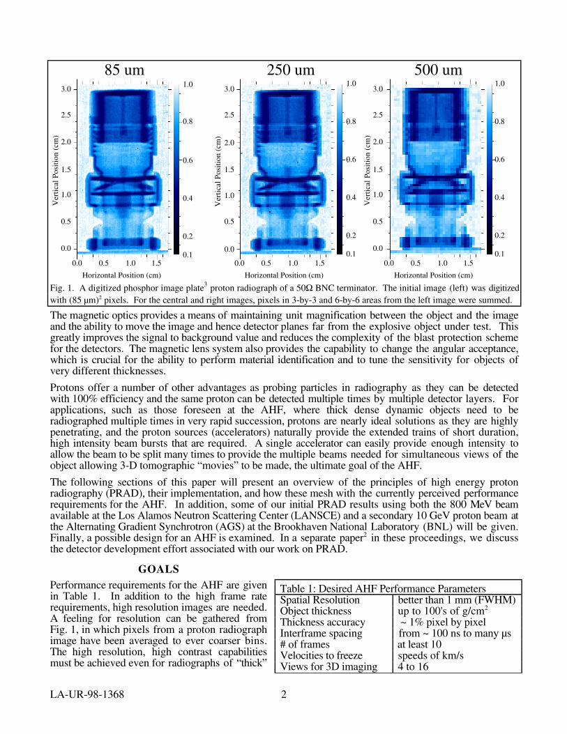
GOALSPerformance requirements for the AHF are givenin Table 1. In addition to the high frame raterequirements, high resolution images are needed.A feeling for resolution can be gathered fromFig. 1, in which pixels from a proton radiographimage have been averaged to ever coarser bins.The high resolution, high contrast capabilitiesmust be achieved even for radiographs of “thick”

Table 1: Desired AHF Performance ParametersSpatial Resolution better than 1 mm (FWHM)Object thickness up to 100's of g/cm2

Thickness accuracy ~ 1% pixel by pixelInterframe spacing from ~ 100 ns to many µs# of frames at least 10Velocities to freeze speeds of km/sViews for 3D imaging 4 to 16

85 um 250 um 500 um

0.0 0.5 1.0 1.5

Horizontal Position (cm)

0.0 0.5 1.0 1.5

Horizontal Position (cm)

0.0 0.5 1.0 1.5

Horizontal Position (cm)

0.0

0.5

1.0

1.5

2.0

2.5

3.0

Ver

tical

Pos

ition

(cm

)

0.0

0.5

1.0

1.5

2.0

2.5

3.0

Ver

tical

Pos

ition

(cm

)

0.0

0.5

1.0

1.5

2.0

2.5

3.0

Ver

tical

Pos

ition

(cm

)

0.1

0.2

0.4

0.6

0.8

1.0

0.1

0.2

0.4

0.6

0.8

1.0

0.1

0.2

0.4

0.6

0.8

1.0

Fig. 1. A digitized phosphor image plate3 proton radiograph of a 50Ω BNC terminator. The initial image (left) was digitizedwith (85 µm)2 pixels. For the central and right images, pixels in 3-by-3 and 6-by-6 areas from the left image were summed.

LA-UR-98-1368 3

objects, where “thick objects” are measured in units of 100’s of g/cm2. Thick objects strongly attenuatethe beam of probing particles in their region of maximum thickness, and potentially produce large amountsof background by scattering particles from thinner regions of the object into the area of the imagecorresponding to the thickest part of the object where few direct particles penetrate. Background issues arefurther complicated by the need to view the object simultaneously from several directions, leading to thepotential for scattering particles from one source into the detectors corresponding to another source. Tiedto the requirement for high precision measurements is the desire to obtain maximum precision with alimited budget of probing particles. This is further constrained by the dynamic range of the detectorsystem, which must count the number of transmitted particles in both the thin and thick regions of theobject. In the following section, the properties of the ideal probing particle will be derived, and we willshow that protons come very close to being such particles.

DESIRED PARTICLE ATTENUATION LENGTH

With a fixed budget of incident particles, one can calculate the ideal attenuation length (λ) for the probingparticles when radiographing an object of a given thickness (L). The ideal attenuation length will be theone that minimizes the fractional error in the difference between the number of particles transmitted by tworegions of the object that differ in thickness by an amount T. We start by assuming simple exponentialattenuation of the beam by the object

N(L) = Noexp(–L/λ), (1)where No is the number of incident particles per pixel, which is assumed to be known. The difference inthe number of particles transmitted through the two regions is given by

N(L) – N(L+ T) = Noexp(–L/λ) – Noexp(–(L+T)/λ) = Noexp(–L/λ) [1 – exp(–T/λ)]. (2)The error in the result given by eq. (2) is simply the square root of the sum of the squares of the errors ineach of the terms in the difference. Since, from counting statistics, the square of the error in N(L) issimply N(L), we have

error in difference = [N(L) + N(L+ T)]1/2 = [Noexp(–L/λ)]1/2 [1 + exp(–T/λ)]1/2. (3)In the limit of T → 0, exp(–T/λ) → 1 – T/λ, and eqs. (2) and (3) become respectively

N(L) – N(L+ T) = Noexp(–L/λ) [T/λ] (4)

error in difference = [N(L) + N(L+ T)]1/2 = [Noexp(–L/λ)]1/2 [2]1/2. (5)Taking the ratio of eq. (5) to eq. (4) in order to get the fractional error gives

fractional error in difference = [2Noexp(–L/λ)]1/2 / Noexp(–L/λ) [T/λ] = 21/2T–1λNo–1/2exp(L/2λ). (6)

Taking the derivative of that with respect to λ and setting the result to zero in order to find the value of λthat minimizes the fractional error gives

(d/dλ ) [fractional error in difference] = (2No)–1/2T–1exp(L/ 2λ) [1 – L/2λ] = 0. (7)

Solving for λ, we findλ = L / 2, (8)

namely the optimal attenuation length is one half the object thickness. Thus for thick objects measured inunits of 100’s of g/cm2, one wants attenuation lengths measured in the same units, not in 10’s of g/cm2.Table 2 gives nuclear interaction lengths for high energy protons (above kinetic energies of ~800 MeVnuclear interaction length values are largely energy independent) and attenuation lengths for 5 MeV x-rays(which have approximately the maximum penetrating depths in high Z materials). Also presented are theresulting fractional error in difference values as calculated using eq. (6) and assuming No = 100,000 andT = 0.01*L (i.e. a 1% thickness difference effect). Since this fractional error must be less than one forthere to be any chance of seeing the thickness difference, the table clearly demonstrates the advantage ofprotons for thick, high Z objects.

MULTIPLE COULOMB SCATTERING

Unlike x-rays, protons undergo a random walk as they pass through an object due to the myriad of smallangle charged particle collisions they have with the atoms in the object. This multiple Coulomb scattering(MCS), at first glance appears to be a great disadvantage for proton radiography since the protons no

LA-UR-98-1368 4

longer travel in a straight line, and an image, unless taken immediately downstream of the object, will beblurred because of the angular dispersion. (Even immediately downstream of the object, some blurringdue to the random walk will be evident.) To first order, the plane projected MCS angular distribution ofthe protons leaving the object is a Gaussian characterized by a root mean square (rms) plane projectiondeflection angle θo which is given by the expression4

θo(z) = 0.0136 GeV (βcp)–1 (z/Xo)1/2 [1 + 0.038 ln(z/Xo)] (9)

where c is the velocity of light, β c is the velocity of the proton, p is its momentum, and z/Xo is thethickness of the object, z, measured in units of radiation length, Xo. It should be noted that as the β of theproton approaches one, θo depends inversely on the momentum of the proton, and only grows as thesquare root of the object thickness. (The logarithmic term is on the order of 10% and has been ignoredhere.) The MCS has two effects. The first is the random walk itself, which leads to the limited blurringpreviously mentioned and is characterized by plane projection rms deviation, y, of the proton from itsunscattered location by the time it reaches the end of the object. That is given by

y(z) = 3–1/2 z θo(z). (10)The second is the additional blurring due to the random direction of the protons from MCS as they leavethe object and travel to the detector, which will be located a non-zero distance from the object. The firsteffect can be dealt with by simply raising the proton beam momentum. To set the scale, for proton beamsof 2, 5, 20, and 50 GeV/c beam, for a 20 radiation length object which is 10 cm thick, y = 2.16, 0.80,0.20, and 0.08 mm respectively. As seen from eqs. (9) and (10), the results improves linearly as thebeam momentum is increased, but grow worse as the product of the linear thickness of the object and thesquare root of the thickness of the object in radiation lengths. Since the object one wants to radiograph hasa known thickness, by choosing a sufficiently high momentum, the blur can be reduced to any desiredvalue. The rms angles θo for the same geometry and beam momenta are 37.4, 13.8, 3.4, and 1.4milliradians respectively. Since we intend to look at explosively driven dynamic objects, the detectorsneed to be quite distant from the object. Thus the second effect must be dealt with by a different means.The solution here relies on the fact that protons are charged and therefore their trajectories can be bent by amagnetic field. More specifically, one builds a magnetic lens. The center of the object is then placed at theobject plane of the long focal length magnetic lens. Similar to an optical lens, the magnetic lens collects allthe protons within its solid angle acceptance, and, regardless of their angle of emission from a point in theobject plane, puts them all back at the corresponding point in the image plane.

MAGNETIC LENS AND MATERIAL IDENTIFICATION

The overall magnetic lens system we have designed5 is shown schematically in Fig. 2. The two imaginglens cells thereof are inverting identity (–I) lenses. These cells are each comprised of four identicalquadrupole magnets operated at identical field strengths, but alternating polarities (+ – + –). They have thefeature that at the center of the gap between the two middle magnets of a cell, the protons are sortedradially solely by their scattering angle in the object, regardless of which point in the object plane theyoriginated from. This allows one to place a collimator at that location and use it to make cuts on the MCS

Table 2: Nuclear interaction lengths for protons and x-ray attenuation lengths4 and the fractional error indifference values for a 1% thickness difference and 100,000 incident particles per pixel.

High Energy Protons (~≥ 1 GeV) 5 MeV x-raysmaterial hydrogen graphite iron lead hydrogen graphite iron lead

λ (g/cm2) 5 0 . 8 8 6 . 3 131 .9 194 .0 21 38 34 23 Xo (g/cm2) 63.05 42.70 13.84 6 .37 L (g/cm2)

1 0 2 .51 4 .09 6 .13 8 .90 1.19 1 .94 1 .76 1.28 2 0 1 .38 2 .17 3 .18 4 .57 0.76 1 .11 1 .02 0.79 5 0 0 .74 1 .03 1 .43 1 .97 0.62 0 .66 0 .63 0.61

1 0 0 0 .61 0 .69 0 .86 1 .12 1.02 0 .63 0 .66 0.90 2 0 0 0 .81 0 .61 0 .63 0 .73 5.49 1 .18 1 .44 3.98 5 0 0 6 .23 1 .40 0 .79 0 .63 2779.31 24.46 47.46 1081.10

LA-UR-98-1368 5

angle in the object. As noted previously, the scattering angle distribution is approximately a Gaussian witha width, which, by eq. (9), depends on the number of radiation lengths of material the protons passedthrough. With the collimator, one can limit the transmitted particles to only those with an MCS angle lessthan the cut angle (θc). The number of transmitted particles Nc after such a cut is given by

N N d Nco o

c c

o

1

2exp

2 1 exp

2 0≈ −

≈ − −

∫ πθ

θθ

θθ

θ 2

2

2

2Ω , or N

Nc c

o

≈ − −

12

2exp

2

θθ

(11)

where N is the number of incident particles. Note that when θc >> θo, Nc = N, as expected. Using eq. (9)for θo, ignoring the small logarithmic term, and solving for z/Xo gives

z

X

cp

N

N

o

c

c

. ln

≈−

−

θ

β

2

213 6

12MeV

(12)

If we now build a lens system which consists of two of the –I lenses set back to back, the first with anaperture sufficient to pass essentially all the particles scattered by MCS (but not those scattered by inelasticnuclear interactions), the second with its aperture set so that it cuts into the MCS distribution, and thenplace detectors at the image planes of the two lenses, we get two independent measurements. The firstdepends on the number of nuclear interaction lengths of material in the object, while the second dependson the number of radiation lengths of material in the object. Since the values of nuclear interaction lengthand radiation length have different dependencies on material type as shown in Table 2, we are in a positionto determine both the amount of material in the object and what that material is. If the object has transitionsfrom one material type to two material types and then from two to three material types, ..., we can unfoldthe object in terms of material types and thickness for each material. (Note that a 1 to 2 material stepfollowed by a 2 to 3 material step can be unfolded, but a sudden 1 to 3 material step cannot be unfolded.)

It should also be noted that by using a single magnetic lens with just a MCS angle cut, one can achievehigh contrast proton radiography even when the object is too thin to provide good contrast using nuclearattenuation. Just as was the case for nuclear exponential beam attenuation, for pure MCS basedradiography of a given thickness object, there is an ideal cut angle that maximizes sensitivity to changes inobject thickness. The value of that optimal cut angle can be determined by the same process as lead to eq.(8), but for an attenuation that is given by eq. (11). Thus by changing the aperture to provide that optimal

Aperture 2Imaging Cell 2DiffuserUpstream Elements

(Matching Lens)ObjectPlane

ImagePlane 1

ImagePlane 2

Aperture 1Imaging Cell 1

X – plane

Y – plane

Fig. 2 Schematic of the PRAD magnetic lens system showing both the X and Y views. The beam is first prepared with adiffuser and matching lens to meet optics requirements. It then passes through the object being radiographed. Thetransmitted beam passes through an iris, or aperture located in the middle of the 4-quadrupole –I magnetic lens cell and isfocused on the first detector. It then enters the second identical –I lens cell, which this time has a smaller diameter iris, andis focused on a second detector. Together, the two detectors provide the information needed to reconstruct both the densityprofile and material composition of the object.

LA-UR-98-1368 6

MCS angle cut, one can tune the system to provide optimum sensitivity, regardless of the object thickness.This was done for the image shown in Fig. 1.

As can be seen in Fig. 2, the magnetic lens system has some additional elements upstream of the object.The proton beam passes through a thin diffuser, which gives a small angular divergence to the beam andthen passes through a set of magnets, which introduces a correlation between the radial position of aproton in the object plane and its angle. This is done to reduce magnetic lens induced aberrations in theidentity lens cells. These aberrations are both geometric and chromatic in nature. For the particularmomentum to which the lens is tuned, the relation between the location of a particle in the object plane,xobject, and its location in the image plane, ximage, for a magnetic lens is given by

ximage = R11xobject + R12φx, (13)where φx is the angle of the particle in the x-plane relative to the axis of the lens, and the R’s are constants,which characterize the magnetic lens. A similar equation holds for the y-coordinate. If instead of havingbeam particles with a single momentum (p), the particles have a spread in momentum, δp, eq. (13)becomes

ximage = (R11 + ∆R11´ + higher order terms)xobject + (R12 + R12´∆ + higher order terms) φx, (14)where ∆ ≡ δp/p and the R´ coefficients are distortion constants for the lens. When an object is placed inthe object plane, several things happen to the transmitted proton beam. First, the protons lose energy andthus momentum; their final average momentum p, being less than their incident momentum po. Themomentum loss in the object is not single valued, but instead covers a range ± δp due to random nature ofthe energy loss process and variations in the thickness of the object. Also, through MCS, an angulardivergence is introduced to the beam, which is characterized by θo, as given by eq. (9).

We are free to arrange the incident proton beam so that all the particles incident on the object plane have arelation between their angle and location in that plane given by φx = wx. Combining this with the effect ofthe MCS, we have φ x = w x + θo for the outgoing beam. Assuming the magnetic lens is tuned to theaverage momentum of the transmitted protons, eq. (14) becomes

ximage = R11xobject + R12φx + (R11´ + wR12´)xobject∆ + R12´θo∆ + higher order terms. (15)Making use of the fact that we have a –I lens, which implies R11 = –1 and R12 = 0, and ignoring the higherorder terms, eq. (15) becomes

ximage = –xobject + (R11´ + wR12´)xobject∆ + R12´θo∆. (16)We note that if we choose w such that w = – R11´/R12´, the xobject∆ term in eq. (16) becomes identicallyequal to zero, and thus all position dependent chromatic aberration terms vanish. The matching magnetsupstream of the object are used to establish that correlation, w, between x and φx. Thus eq. (16) becomes

ximage = –xobject + R12´θo∆, provided: w = – R11´/R12´. (17)In addition to the matching lens establishing the desired correlation between incident particle angle andlocation at the object plane, the lens provides some other useful functions. It further expands the incidentbeam allowing one to illuminate a large object, without making the upstream diffuser very thick. It alsohelps maintain a very uniform acceptance across the full field of view of the imaging lenses.

MOMENTUM SCALING

The remaining distortion term in eq. (17) is given by∆x = xobject + ximage = R12´ θo∆, (18)

which is characterized by the chromatic aberration coefficient of the lens, R12´, and the product θo∆. Forhigh momentum protons (> 1 GeV/c), the momentum loss is essentially independent of beam momentum.Therefore the fractional momentum bite of the beam, ∆, scales inversely proportional to the beammomentum. Likewise from eq. (9), the angle θο is also inversely proportional to the beam momentum.Thus the spatial resolution of the magnetic lens system improves as the square of the beam momentum.

Other factors also effect the overall spatial resolution that can be attained in proton radiography. There isthe spatial resolution of the detector system, which is essentially independent of momentum. There is alsothe effect of the non-zero thickness of the object, which by eq. (10) degrades the resolution. As discussedearlier, this effect scales as 1/p. If there is a vessel to contain the explosive blast in an AHF application,

LA-UR-98-1368 7

the MCS of the incoming and outgoing beams inthe vessel walls will produce a similar effect, butthis time linearly dependent on the separationbetween the object and the containment vesselwall. Due to the relatively large value of thisdistance, this will likely be the dominant termeffecting spatial resolution. The MCS in the vesselwall will change the value of the outgoing protonangle, which cannot be corrected for by themagnetic lens. This characteristic angle changemultiplied by the distance from the object to thevessel wall will be the amount of blur introduced.(If the vessel wall is closer to the image plane thanthe object plane, the relevant distance is the vesselwall to image plane separation.) The characteristicangle involved is again given by eq. (9) and thusscales as 1/p. As eq. (9) also shows, it dependson the thickness of the vessel wall in units ofradiation length, and therefore it is important to usethin, low-Z materials. The vessel wall thickness isless important for the incident beam, since there itaffects the desired correlation between the incidentparticle location at the object and the particle anglethere. This correlation was to remove the

chromatic spatial aberrations from the lens, which were already a higher order effect. In Fig. 3 we plotthe expected overall spatial image blurring as a function of beam momentum for the various terms andvarious containment vessel walls.

PROTON DETECTION

Protons, being charged particles, directly excite the detector medium, predominantly through Coulombinteractions with electrons in the medium. They thus generate a signal even for an extremely thin detector.Because of the mass difference between protons and electrons, there is very little deflection of the protonsby the detector, and therefore very little in the way of a detector produced background problem. Incontrast, x-rays, being uncharged, do not directly ionize the detector material as they pass through it. As amatter of fact, it takes one x-ray attenuation length for 63% of the x-rays to interact and generate a chargedparticle, which then leaves the excitation trail that a detector sees. X-rays predominantly interact throughlarge angle scattering, and due to the large required detector thickness are likely to have secondaryinteractions that produce backgrounds in the detector. Since protons can be detected by very thindetectors, no similar problem exists for them. Also in a thin detector, the proton is virtually undeflectedand therefore can be used for a second (or third) time, such as in a second magnetic lens system for MCSmaterial identification. Furthermore, multiple planes of detectors can detect the same proton, therebyachieving redundancy. The thinness of the proton detectors also makes them essentially blind to neutralsecondary particles generated in the object (neutrons and γ-rays), thereby reducing the potential for otherbackground problems.

BACKGROUNDS

Backgrounds in the case of proton radiography are very small, as we have verified both in Monte Carlostudies and in experiments. This results from the relatively long values of interaction (attenuation) lengthsfor protons and the large standoff distance for the detectors from the object, which is due to the magneticlens system. The magnetic lens also provides filtering of off-momentum background particles. At thesame time, the thin detectors are essentially blind to neutral secondary particles, which would otherwisedominate the relatively small background. In neither proton nor x-ray radiography are the “attenuated”particles cleanly removed from the beam. Some fraction of the “attenuated beam” will undergo one orseveral hard interactions in the object and/or surrounding material and still hit the detector in a location that

0.01

0.10

1.00

10FW

HM

Blu

rrin

g (m

m)

10 15 20 25 30 35 40 45 50 55 60Momentum (GeV/c)

lens

objectdetector

all, 2" steelal l , 2"" aluminum

all, 6" CH2 composite

Fig. 3. The momentum scaling for the various termseffecting spatial resolution. Shown are possible individualcontributions from the detector, object, and lens, and theoverall contribution when these are combined with differentcontainment vessels values.

LA-UR-98-1368 8

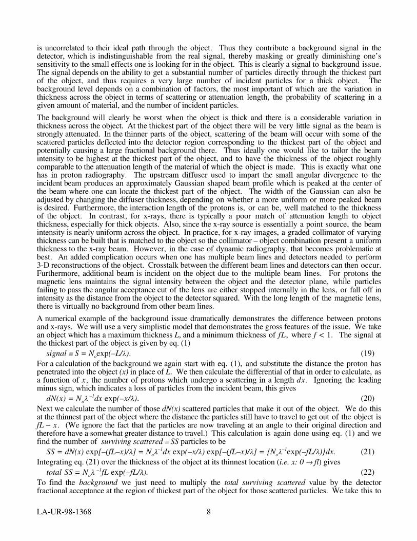
is uncorrelated to their ideal path through the object. Thus they contribute a background signal in thedetector, which is indistinguishable from the real signal, thereby masking or greatly diminishing one’ssensitivity to the small effects one is looking for in the object. This is clearly a signal to background issue.The signal depends on the ability to get a substantial number of particles directly through the thickest partof the object, and thus requires a very large number of incident particles for a thick object. Thebackground level depends on a combination of factors, the most important of which are the variation inthickness across the object in terms of scattering or attenuation length, the probability of scattering in agiven amount of material, and the number of incident particles.

The background will clearly be worst when the object is thick and there is a considerable variation inthickness across the object. At the thickest part of the object there will be very little signal as the beam isstrongly attenuated. In the thinner parts of the object, scattering of the beam will occur with some of thescattered particles deflected into the detector region corresponding to the thickest part of the object andpotentially causing a large fractional background there. Thus ideally one would like to tailor the beamintensity to be highest at the thickest part of the object, and to have the thickness of the object roughlycomparable to the attenuation length of the material of which the object is made. This is exactly what onehas in proton radiography. The upstream diffuser used to impart the small angular divergence to theincident beam produces an approximately Gaussian shaped beam profile which is peaked at the center ofthe beam where one can locate the thickest part of the object. The width of the Gaussian can also beadjusted by changing the diffuser thickness, depending on whether a more uniform or more peaked beamis desired. Furthermore, the interaction length of the protons is, or can be, well matched to the thicknessof the object. In contrast, for x-rays, there is typically a poor match of attenuation length to objectthickness, especially for thick objects. Also, since the x-ray source is essentially a point source, the beamintensity is nearly uniform across the object. In practice, for x-ray images, a graded collimator of varyingthickness can be built that is matched to the object so the collimator – object combination present a uniformthickness to the x-ray beam. However, in the case of dynamic radiography, that becomes problematic atbest. An added complication occurs when one has multiple beam lines and detectors needed to perform3-D reconstructions of the object. Crosstalk between the different beam lines and detectors can then occur.Furthermore, additional beam is incident on the object due to the multiple beam lines. For protons themagnetic lens maintains the signal intensity between the object and the detector plane, while particlesfailing to pass the angular acceptance cut of the lens are either stopped internally in the lens, or fall off inintensity as the distance from the object to the detector squared. With the long length of the magnetic lens,there is virtually no background from other beam lines.

A numerical example of the background issue dramatically demonstrates the difference between protonsand x-rays. We will use a very simplistic model that demonstrates the gross features of the issue. We takean object which has a maximum thickness L, and a minimum thickness of fL, where f < 1. The signal atthe thickest part of the object is given by eq. (1)

signal ≡ S = Noexp(–L/λ). (19)For a calculation of the background we again start with eq. (1), and substitute the distance the proton haspenetrated into the object (x) in place of L. We then calculate the differential of that in order to calculate, asa function of x, the number of protons which undergo a scattering in a length dx. Ignoring the leadingminus sign, which indicates a loss of particles from the incident beam, this gives

dN(x) = Noλ –1dx exp(–x/λ). (20)Next we calculate the number of those dN(x) scattered particles that make it out of the object. We do thisat the thinnest part of the object where the distance the particles still have to travel to get out of the object isfL – x. (We ignore the fact that the particles are now traveling at an angle to their original direction andtherefore have a somewhat greater distance to travel.) This calculation is again done using eq. (1) and wefind the number of surviving scattered ≡ SS particles to be

SS = dN(x) exp[–(fL–x)/λ] = Noλ–1dx exp(–x/λ) exp[–(fL–x)/λ] = Noλ–1exp(–fL/λ)dx. (21)Integrating eq. (21) over the thickness of the object at its thinnest location (i.e. x: 0 → fl) gives

total SS = Noλ –1fL exp(–fL/λ). (22)To find the background we just need to multiply the total surviving scattered value by the detectorfractional acceptance at the region of thickest part of the object for those scattered particles. We take this to

LA-UR-98-1368 9

be H. Thus we find the signal to background value ≡ S/B is given byS/B = Noexp(–L/λ) / [H Noλ –1fL exp(–fL/λ)] = λ(HfL)–1exp[–(1–f)L/λ]. (23)

In Table 3 are given some values of the S/B for different materials, values of L, and values of f, both for5 MeV x-rays and high energy protons. Also given are the beam transmission probabilities (S/No) at thethickest part of the object. We take H = 0.001. It should be noted that due to the limited momentumtransmission of the magnetic lens in proton radiography, the value of H for protons should be less thanthat for x-rays, improving the S/B value for protons relative to that for x-rays beyond the values shown.

A related issue addressed in Table 3 is the dynamic range required for the detector. If a uniform intensitybeam is incident on the object, the ratio, R, of the signal intensity at the thinnest part of the object to that atthe thickest part of the object (ignoring background) is given by

R = Noexp(–fL/λ) / [No exp(–L/λ)] = exp( (1–f)L/λ). (24)As Table 3 shows, R can be quite large for x-rays, especially when λ is small compared to L. In lookingat these values and considering the detector dynamic range and sensitivity, it is important to keep in mindthat the detector must, in addition, be able to see on the order of a 1% change in object thickness at thethickest part of the object.

The preceding calculations do not deal with the production of secondary particles in the object due tonuclear interactions. We examined this issue in a Monte Carlo study which used the latest version of theLAHET6 code, which in turn uses FLUKA7 to simulate the nuclear scattering and particle secondaryproduction. In the study, a zero diameter beam of 50 GeV protons was incident normal to a slabs of 238Uof different thicknesses. At the downstream face of the slab we recorded all outgoing particles. For thoseparticles, their particle type, location, and 3-momentum were recorded. Neutrons were tracked down tokinetic energies of 20 MeV. Due to the inability of LAHET to directly deal with γ-rays, and electrons andpositrons, these were ignored. The predominant source of γ-rays will be πo decays, whose number willbe about the same as those for π+ or π–, the dominant secondary charged particles. As the πo decaysessentially instantaneously, into two γ-rays, by the above arguments, their number will initially be aboutequal to the number of secondary charged particles. However, the γ-rays will be strongly attenuated in theobject, and the few surviving γ-rays will be spread over a large angular region and thus outside the angularacceptance of the magnetic lens system. Since they are also nearly invisible to the detectors, their omissionshould have a negligible effect on the results. Fig. 4 gives the angular distribution of all the particlesmaking it out of the back of the slab sorted by particle type. Fig. 5 shows a similar plot, but for outgoingparticle momentum. Both figures are for 500 g/cm2 of uranium, a very thick object, where the backgroundproblem will be most severe. In Table 4, we record the signal and background values for cuts on theoutgoing particle angle and momentum for different slab thicknesses. We consider signal particles to beprotons which have angles inside the outgoing angle cut, and a momentum which is greater than theexpected average momentum of protons exiting the slab minus 5%. As can be seen, secondary particlescontribute very little, and the dominant secondary particles are neutral and thus essentially invisible to thedetector.

Table 3: Signal to background values assuming H = 0.001.material λnuclear λ5 MeV x–ray L f (S/No)nuclear (S/No)x-ray S/Bnuclear S/Bx-ray Rnuclear Rx-ray

(g/cm2) (g/cm2) (g/cm2)iron 131.9 34 304 0.2 0.1 1.32E-04 3 4 4 0 . 4 6.3 1269.2iron 131.9 34 212 0.2 0.2 1.94E-03 8 5 7 5 . 4 3.6 147.7iron 131.9 34 9 1 0.2 0.5 6.79E-02 4143 216.3 1.7 8.6iron 131.9 34 304 0.5 0.1 1.32E-04 2 7 5 2 . 6 3.2 87.0iron 131.9 34 212 0.5 0.2 1.94E-03 5 5 6 14 .1 2.2 22.7iron 131.9 34 9 1 0.5 0.5 6.79E-02 2040 193.9 1.4 3.8

lead 194.0 23 447 0.2 0.1 3.67E-09 3 4 4 4.60E-05 6.3 5595334.9lead 194.0 23 312 0.2 0.2 1.27E-06 8 5 7 7.07E-03 3.6 52062.9lead 194.0 23 135 0.2 0.5 2.89E-03 4143 8 . 0 1.7 107.5lead 194.0 23 447 0.5 0.1 3.67E-09 2 7 5 6.24E-03 3.2 16496.5lead 194.0 23 312 0.5 0.2 1.27E-06 5 5 6 1.66E-01 2.2 886.8lead 194.0 23 135 0.5 0.5 2.89E-03 2040 18 .4 1.4 18.6

LA-UR-98-1368 10

EXPERIMENTAL WORK

We have carried out a number of experimental tests of the PRAD concept using magnetic imaging lenses.Some of these tests were carried out at the LANSCE facility, making use of its 800 MeV chopped protonbeam. The 800 MeV beam energy is too low to allow for the study of thick objects in which nuclearattenuation is important. This is due to the large dispersion in momentum loss by the protons at 800 MeV,both directly and as a result of variations in object thickness. As discussed earlier, this results in poor lensperformance and hence a blurred, poor quality image. However, by looking at thinner objects, we couldstill study the MCS part of the PRAD concept, the actual performance of the magnetic lens system, and bymaking use of the pulsed nature of the proton beam (one pulse every N×358 ns, N = integer), take asequence of radiographs of explosively driven events.

The ability to take high contrast, high resolution images using a MCS angle cut for a thin object isdemonstrated by the image shown in Fig. 1, which is a static radiograph taken using a phosphor imageplate as a detector. The object is a 50 Ω BNC terminator that is only 1.4 cm in diameter. The resistor andits leads inside the metal case of the terminator are clearly visible, as are the internal screw threads. Evensubmillimeter features are sharp.Radiographic images of a dynamic event areshown in Fig. 6. The object is a 58 mmdiameter half-sphere of high explosive (HE)which is in the process of detonating. Theseimages were again made with phosphorimage plates. Four different explosive shotswere fired to produce the four radiographs,with the proton beam timed to arrive atdifferent times relative to the detonationinitiation time. The different times are (top tobottom) 0.99 µs, 1.90 µs, 2.50µs, and3.25µs after detonation initiation. Alsoshown are the results of a reconstruction ofthe object from those radiographs. Theposition of the shock front (the glitch inFig. 6) associated with the detonation isseen to progress between the differentradiographs. The shock front is seen tocorrespond to about a 30% increase in local

0.00

1000

2000

3000

Num

ber

0 .0 0.2 0.4 0.6 0.8 1.0 1.2 1.4 1.6

Theta (radians)

neutrals

other charged

protons

0

1000

2000

3000

4000

Num

ber

0.000 0.005 0.010 0.015Theta (radians)

other chargedneutralsprotons

Fig. 4. Histograms of the number of outgoing particles of aparticular type as a function of scattering angle for 100,000incident 50 GeV protons on a 500 g/cm2 slab of 238U.

1.00

10

100

1000

10000

100000

Num

ber

0 5 10 15 20 25 30 35 40 45 50 Momentum (GeV/c)

neutralsprotons

other charged

1

10

100

1000

10000

Num

ber

47.5 48.0 48.5 49.0 49.5 50.0 50.5Momentum (GeV/c)

other chargedneutralsprotons

Fig. 5. Histograms of the number of outgoing particles ofa particular type as a function of momentum for 100,000incident 50 GeV protons on a 500 g/cm2 slab of 238U.

Table 4: Particle generation & survival in the given amount of 238U

no cut 10 mradθ cut

47.9 GeV/cmomentum cut

momentum andθ cut

50 g/cm2

protons 151840 77756 77015 76761 neutrals 211620 633 2 1 1 1 other charged 196658 837 0 0 100 g/cm2

protons 182034 60733 59584 59184 neutrals 448298 1017 3 6 1 4 other charged 331171 1364 0 0 200 g/cm2

protons 212593 36998 35597 35134 neutrals 883247 1318 4 5 2 3 other charged 473650 1691 0 0 500 g/cm2

protons 168694 8209 7473 7160 neutrals 1319912 935 1 1 5 other charged 397354 1044 0 0

LA-UR-98-1368 11

density. Behind the shock front a rarefaction can also be seen. For the above images, the collimatorinside the magnetic lens was set to provide a MCS angle cut of 10 milliradians.

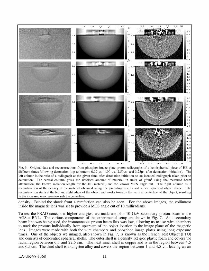
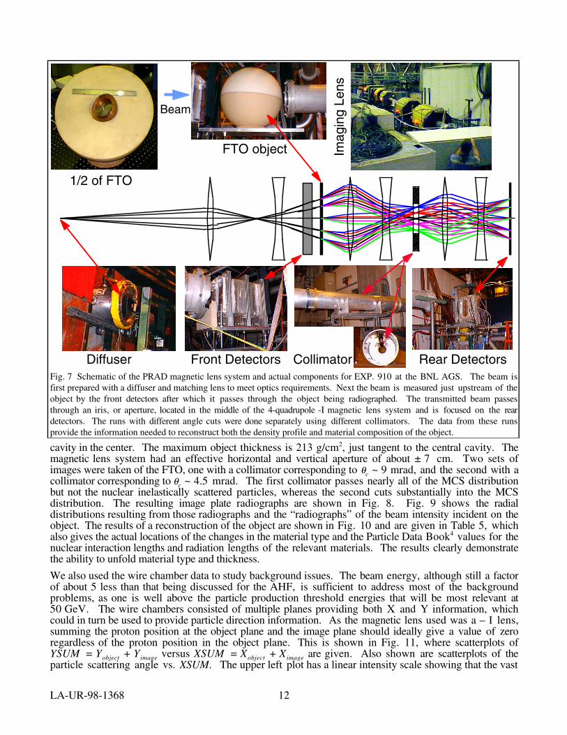
To test the PRAD concept at higher energies, we made use of a 10 GeV secondary proton beam at theAGS at BNL. The various components of the experimental setup are shown in Fig. 7. As a secondarybeam line was being used, the instantaneous proton beam flux was low, allowing us to use wire chambersto track the protons individually from upstream of the object location to the image plane of the magneticlens. Images were made with both the wire chambers and phosphor image plates using long exposuretimes. One of the objects we imaged, also shown in Fig. 7, is known as the French Test Object (FTO)and consists of concentric spherical shells. The outer shell is a density 1/2 g/cc plastic foam and covers theradial region between 6.5 and 22.5 cm. The next inner shell is copper and is in the region between 4.5and 6.5 cm. The third shell is a tungsten alloy and covers the region between 1 and 4.5 cm leaving an air

Fig. 6. Original data and reconstructions from phosphor image plate proton radiographs of a hemispherical piece of HE atdifferent times following detonation (top to bottom: 0.99 µs, 1.90 µs, 2.50µs, and 3.25µs after detonation initiation). Theleft column is the ratio of a radiograph at the given time after detonation initiation to an identical radiograph taken prior todetonation. The central column gives the unfolded amount of material in units of g/cm2 using the measured beamattenuation, the known radiation length for the HE material, and the known MCS angle cut. The right column is areconstruction of the density of the material obtained using the preceding results and a hemispherical object shape. Thereconstruction starts at the left and right edges of the object and works towards the vertical centerline of the object, resultingin the increased error seen towards the centerline.

LA-UR-98-1368 12

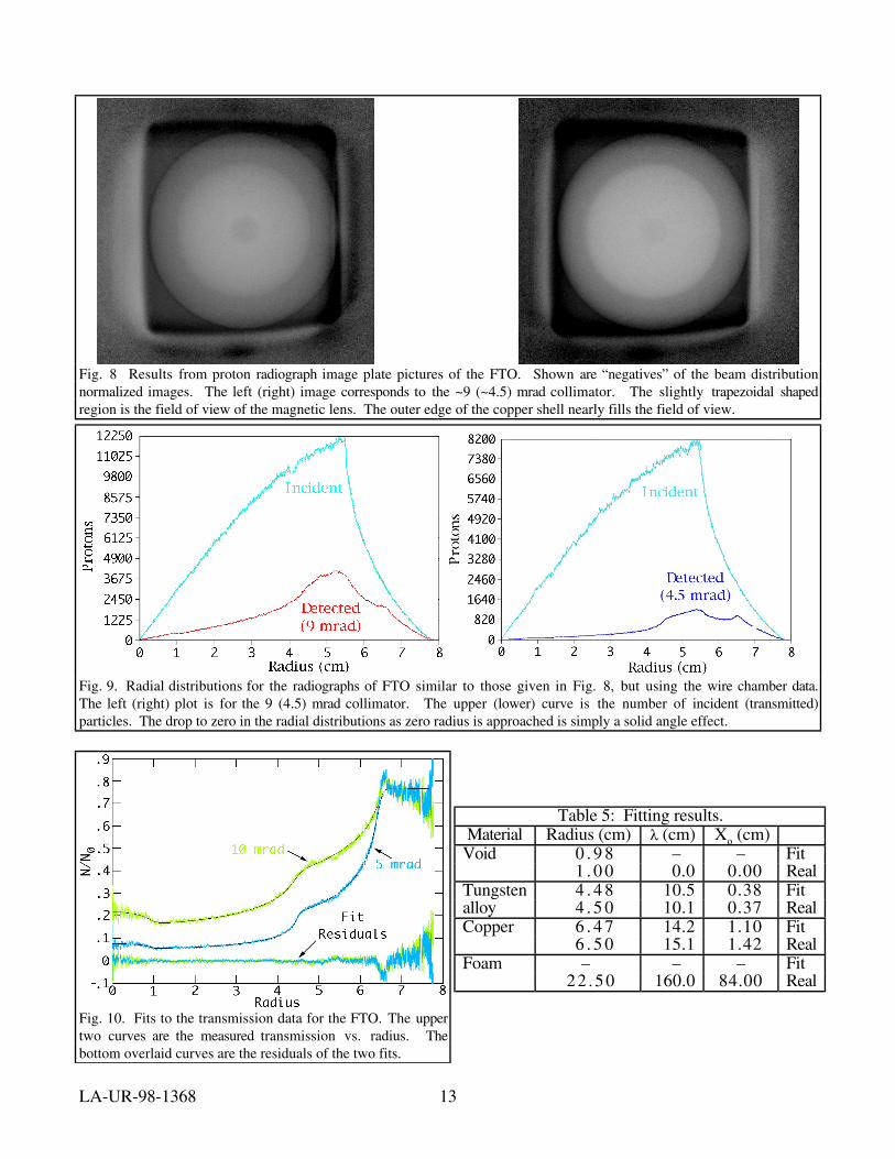
cavity in the center. The maximum object thickness is 213 g/cm2, just tangent to the central cavity. Themagnetic lens system had an effective horizontal and vertical aperture of about ± 7 cm. Two sets ofimages were taken of the FTO, one with a collimator corresponding to θc ~ 9 mrad, and the second with acollimator corresponding to θc ~ 4.5 mrad. The first collimator passes nearly all of the MCS distributionbut not the nuclear inelastically scattered particles, whereas the second cuts substantially into the MCSdistribution. The resulting image plate radiographs are shown in Fig. 8. Fig. 9 shows the radialdistributions resulting from those radiographs and the “radiographs” of the beam intensity incident on theobject. The results of a reconstruction of the object are shown in Fig. 10 and are given in Table 5, whichalso gives the actual locations of the changes in the material type and the Particle Data Book4 values for thenuclear interaction lengths and radiation lengths of the relevant materials. The results clearly demonstratethe ability to unfold material type and thickness.

We also used the wire chamber data to study background issues. The beam energy, although still a factorof about 5 less than that being discussed for the AHF, is sufficient to address most of the backgroundproblems, as one is well above the particle production threshold energies that will be most relevant at50 GeV. The wire chambers consisted of multiple planes providing both X and Y information, whichcould in turn be used to provide particle direction information. As the magnetic lens used was a – I lens,summing the proton position at the object plane and the image plane should ideally give a value of zeroregardless of the proton position in the object plane. This is shown in Fig. 11, where scatterplots ofYSUM = Yobject + Yimage versus XSUM = Xobject + Ximage are given. Also shown are scatterplots of theparticle scattering angle vs. XSUM. The upper left plot has a linear intensity scale showing that the vast

Diffuser Front Detectors Rear DetectorsCollimator

Imag

ing

Lens

Beam

1/2 of FTO

FTO object

Fig. 7 Schematic of the PRAD magnetic lens system and actual components for EXP. 910 at the BNL AGS. The beam isfirst prepared with a diffuser and matching lens to meet optics requirements. Next the beam is measured just upstream of theobject by the front detectors after which it passes through the object being radiographed. The transmitted beam passesthrough an iris, or aperture, located in the middle of the 4-quadrupole -I magnetic lens system and is focused on the reardetectors. The runs with different angle cuts were done separately using different collimators. The data from these runsprovide the information needed to reconstruct both the density profile and material composition of the object.

LA-UR-98-1368 13

Fig. 8 Results from proton radiograph image plate pictures of the FTO. Shown are “negatives” of the beam distributionnormalized images. The left (right) image corresponds to the ~9 (~4.5) mrad collimator. The slightly trapezoidal shapedregion is the field of view of the magnetic lens. The outer edge of the copper shell nearly fills the field of view.

Fig. 9. Radial distributions for the radiographs of FTO similar to those given in Fig. 8, but using the wire chamber data.The left (right) plot is for the 9 (4.5) mrad collimator. The upper (lower) curve is the number of incident (transmitted)particles. The drop to zero in the radial distributions as zero radius is approached is simply a solid angle effect.

Fig. 10. Fits to the transmission data for the FTO. The uppertwo curves are the measured transmission vs. radius. Thebottom overlaid curves are the residuals of the two fits.

Table 5: Fitting results.Material Radius (cm) λ (cm) Xo (cm)Void 0 . 9 8 – – Fit

1 . 0 0 0.0 0.00 RealTungsten 4 . 4 8 10.5 0.38 Fitalloy 4 . 5 0 10.1 0.37 RealCopper 6 . 4 7 14.2 1.10 Fit

6 . 5 0 15.1 1.42 RealFoam – – – Fit

22 .50 160.0 84.00 Real

LA-UR-98-1368 14

Fig. 11. Top left: two-dimensional histogram of XSUM vs. YSUM on a linear scale; top right on a logarithmic scale;bottom left: XSUM vs. scattering angle on a linear scale; bottom right: on a logarithmic scale with the additional restrictionthat both |XSUM| and |YSUM| be larger than 5 mm.

majority of events are not “problem” events. The upper right plot is the same data, but plotted on alogarithmic intensity scale to highlight the “problem” events. The bottom left plot shows on a linearintensity scale the proton scattering angle in the object as a function of XSUM and demonstrates that thelens also performs well over the relevant range of scattering angles. The bottom right plot shows the samedistribution but on a logarithmic intensity scale and only for “problem” events. The “problem” orbackground events are defined as those that have both |XSUM| > 5 mm and |YSUM| > 5 mm. (Thisexplains the missing events in the |XSUM| ≤ 5 mm region of the plot.) The information on background ismore qualitatively given in the histograms shown in Fig. 12. The events shown are from a radiograph ofthe FTO, where only those events that at the object plane were within a horizontal band of ± 5 mm heightcentered on the FTO were used. It should be noted that the events considered passed all the way throughto the imaging lens and to a trigger counter located behind the wire chambers at the image plane. (Thisexplains the shape of the object plane distributions in Fig. 12, where the central air cavity and copper totungsten transitions are evident.) The left column gives the X-distribution of those particles measured atthe object plane, whereas the right column is for the same particles, but measured at the image plane. Eachplot has two curves. The upper curve (darker) curve is for all events, whereas the lower (lighter) curve isfor the background events as defined previously. There were several problems with the experimentalsetup which caused larger than expected backgrounds. One problem was inadequate shielding upstream ofthe object which allowed particles outside the “field of view” of the upstream lens to reach the object andimage plane. Another problem was that the incident beam was by mistake not centered on the object; themajority of the beam actually missing the object and hitting the upstream magnets. The third problem wasinadequate thickness for the collimator, which allowed some of the protons that hit the collimator to stillreach the image plane. With the use of the wire chamber data, these types of events could be removed.This is shown in the lower two rows of histograms in Fig. 12. The measured “expected” background tosignal values can be read off of the bottom row histograms and are on the order of a few percent. A morecareful set-up would no doubt have improved these values.

LA-UR-98-1368 15

AHF PROTON ACCELERATOR COMPLEX

The AHF will be required to produce transmission radiographic images with high spatial and temporalresolution From 4 to 16 simultaneously-illuminated views and 25 or more time-separated exposures perview are desired. The desired beam-pulse structure needs to be flexible, with 1010 to 1011 protons in a 10-20 nsec-long pulse per view. A programmable time separation between pulses in each view which variesfrom a minimum of about 100 nsec to a maximum of many microseconds. These requirements lead to theuse of a low-duty-factor, slowly cycling proton synchrotron with a flexible multipulse beam-extractionsystem, feeding into a multistage beam-splitting transport system that transmits proton pulses to the testfacility.

The total number of protons in the ring is approximately 1013. This number follows from the followingarguments. If we want pixel by pixel measurements that have an accuracy of 1 part in A , we need A2

particles per pixels from counting statistics arguments alone. Allowing for other measurement errors suchas those associated with the detectors, we need to boost the number of particles by a factor of B . Thebeam is attenuated by the object by a factor of C, thus we need A2BC particles per pixel in the incidentbeam. Taking into account the area of the object we need an additional factor D given by (area of object) /(area of a pixel). If we now have E views, assume losses in the beam splitting chain are a factor of Foverall, and record G frames per view, the machine must deliver A2BCDEFG protons in a shot. Goingback to Table 1, and taking round number values, we have A ~ 100, B ~ 2, C ~ 5 (the Gaussian shaped

Fig. 12. Left: histograms of X positions at the object plane for events within a 1 cm high band in Y centered on the FTO atthe object plane. Right: histograms of positions at the image plane. Top: all events. Middle: events required to be in thelens field of view at the object. Bottom: events also required to be within the collimator acceptance. The upper lines are thesignal plus background. The lower lines are the background.

LA-UR-98-1368 16

beam centered on the thickest part of theobject helps here), D ~ (10 cm/250 µm)2 =160,000, E ~ 16 (beam splitting in ourdesign is in multiples of 2), F ~ 2, and G ~25, which approximately yields the 1013

value.

The nominal beam energy of 50 GeV is set by object thickness and also by the thickness of the vessel(windows) that must contain the blast. The present study is based on an 800-MeV linac, such as availableat LANSCE, which injects an H– beam directly into a 50 GeV synchrotron. Numerous protonsynchrotrons in the energy and/or intensity range needed for PRAD are presently in operation around theworld. Thus the technology required for a PRAD accelerator has already been demonstrated. A conceptualpoint design for a system that can meet the above requirements has been presented elsewhere8. Thesynchrotron is fairly conventional, except for use of a lattice with an imaginary transition γ and certainfeatures of the achromatic arcs.

There are two design parameters of a PRAD synchrotron that need some particular attention. First,simplicity of operation and low intensity suggests that a booster stage can be avoided. However, a criticalparameter is the magnetic field at injection time. For a 50 GeV synchrotron operating at 1.7 Tesla at fullenergy, the magnetic field at injection time with 800 MeV injection is 0.05 Tesla. This is thought to beabout the minimum practical field. Thus 50 GeV is the maximum practical energy for injection by theexisting LANSCE linac at Los Alamos. For a higher energy PRAD synchrotron, either a boostersynchrotron, or a higher energy injection linac would be required. (If constructed on a greenfield site, alower energy linac plus a small booster would be a more cost-effective injector solution.)

The second issue concerns beam extraction from the high-energy synchrotron. If single-turn extraction ischosen, then a pulse train of length equal to the circumference of the synchrotron is delivered to theexperiment. For a 1.5 km typical circumference of a 50 GeV synchrotron, this amounts to a total pulsetrain length of 5 microseconds. The bunch frequency in this train is the rf frequency of the synchrotron.We presently favor a 5 MHz rf frequency, thus providing bunch spacing of 200 ns. Loss-less extractionis possible if the kicker rise time is less than 200 ns, which is obtainable with today’s technology.

If single-bunch extraction were to be installed, it would be possible to make a quite flexible program ofpulse delivery that extends from spacing of 200 ns up to seconds. The total number of pulses available inthe reference scheme would be 25 pulses. For this mode of operation, it is likely that a well-terminatedsingle step kicker of 50 Ohm characteristic impedance would be used. For variable proton burst spacing, amodulator capable of providing 25 pulses with variable pulse spacing would have to be developed.Although no such modulator presently exists, it is believed that its development is not likely to present anyobstacles to construction of the facility.

Both beam transport and beam splitting are performed in the beam transport system (see Fig. 13). Thebeamlines are achromatic and isochronous; the latter feature is enforced by symmetry. In the presentexample, there are 12 beamlines illuminating the target from different angles, both in-plane and out-of-plane. At the end of each beamline, there is a 45-m target-illuminating section that includes a diffuser andmagnetic quadrupoles that prepare the beam size and convergence angles for object illumination. On theopposite side of the object containment chamber from each illuminating section, there are magnetic imaging

Table 6. Twelve-View Beamline SummaryTotal splitter sections 4Total straight cells 120Total bend cells 232Quadrupole Length (m) 704bore radius (cm) 0.5gradient (T/m) 2.5Number of Dipoles 928Dipole Length (m) 2.0gap (cm) 5.0field (T) 4.2

LINAC

50 GeV Ring

20 GeV Booster

Splitter Splitter

Splitter

Splitter0 scale 1000 m

Imagers

V

Fig. 13. Layout of the entire facility for 12 views, showing thelinac, booster, main ring, and beamlines.

LA-UR-98-1368 17

systems and detector arrays. The transport system parameters for the above design are listed in the Table 6exclusive of the matching and imaging lenses.

CONCLUSION

We have reviewed the basic concept of proton radiography and found that it should perform extremelywell and have substantial advantages of x-ray based radiography in the case of thick (100’s g/cm2) objects.In the case of thin objects, it still performs very well, with added bonus that it can be tuned to give highcontrast images regardless of how thin the object is. An added feature of proton radiography is the abilityto measure, not only the amount of material (as in standard radiography), but also the composition of theradiographed object in terms of material identities. These predictions have been confirmed in beam tests.The proton accelerator needed for a future Advanced Hydrotest Facility is not beyond the scope of existingproton accelerators. Furthermore proton accelerators naturally have the strobed pulse nature needed tofollow rapidly evolving dynamic events and can do so for an extended period of time.

1 InterScience, Inc., “Technology Review of Advanced Hydrodynamic Radiography”, March 6-7, 1996, ISI-TM96050701.93.2 H.-J. Ziock et al., “Detector Development for Dynamic Proton Radiography”, these proceedings.3 J. Miyahara et al., “A New Type Of X-Ray Area Detector Utilizing Laser Stimulated Luminescence”, Nucl. Instr. andMeth., A246 (1986) 572.

4 Particle Data Group, “Review of Particle Physics”, Phys. Rev. D54, (1996).5 C.T. Mottershead and J. D. Zumbro, “Magnetic Optics for Proton Radiography”, Proceedings of the 1997 Particle

Accelerator Conference, Vancouver, B. C., Canada (to be published).6 R. E. Prael, H. Lichtenstein, et. al., “User Guide to LCS: The LAHET Code System”, LA-UR-3014, (1989). For moreinformation see http://www-xdiv.lanl.gov/XCI/PROJECTS/LCS/ or contact R. Prael (505)667-7283.

7 A. Fasso, A. Ferrari, J. Ranft, P.R. Sala, G. R. Stevenson, J.M. Zazula, ”A Comparison of FLUKA Simulations withMeasurements of Fluence and Dose in Calorimeter Structures”, Nucl. Instr. and Meth. , A332 (1993) 459.

8 F. A. Neri, H. A. Thiessen, and P. L. Walstrom, “Synchrotrons and Beamlines for Proton Radiography”, Proceedings of the1997 Particle Accelerator Conference, Vancouver, B. C., Canada (to be published).