the process of statistical...
TRANSCRIPT

UNIT OVERVIEW
GOALS AND STANDARDS
MATHEMATICS BACKGROUND
UNIT INTRODUCTION
Mathematics BackgroundThe Process of Statistical Investigation
In Samples and Populations, students use their background knowledge of statistical investigations and probability to draw conclusions about samples and populations. Statistical investigations involve four parts:
• Posing questions
• Collecting data
• Analyzing data distributions
• Interpreting the data and the analysis to answer the questions
At the end of a statistical investigation, students need to communicate the results.
Students learned about data and statistical measures in Grade 6 during Data About Us. There are opportunities in Investigation 1 to review the Grade 6 content. The focus of Samples and Populations, however, is not on reviewing the material introduced in Grade 6. The focus is to extend the concepts developed in Grade 6. You should gauge whether or not your students would benefit from an additional quick refresher of concepts.
In Samples and Populations, students will use both data that are provided for them in the Student Edition and data that they generate. In both cases, students need to consider the process of statistical investigation.
When students collect their own data, they naturally tend to follow through with the process of statistical investigation. When students analyze a data set they have not collected, however, they need to understand the data first in order to complete any analysis. Have students think about why and how the data might have been collected.
Questions students should ask themselves• What question might have been asked in order to collect the data?
• How do you think the data were collected?
• Why are these data represented with this kind of display?
• How can you describe the data distribution?
• How can you use the results of the analysis to answer the original question?
13Mathematics Background
CMP14_TG07_U8_UP.indd 13 31/12/13 1:22 AM
Look for these icons that point to enhanced content in Teacher Place
Reviewing Types of Data and Attributes
AttributesIn Samples and Populations students use the word attributes, rather than variables, to describe qualities that certain data have. This is so that students do not confuse statistics concepts with algebra concepts. An attribute names a particular characteristic of a person, place, or thing about which data are being collected. For example, height is an attribute of male professional basketball players.
Categorical and Numerical Data ValuesStatistical questions result in answers that are either categorical or numerical data values.
Numerical data arise from questions for which the answers are numbers, counts, or measurements. For example, “How tall are these basketball players?” will result in answers such as 81 inches.
Categorical data arise from questions for which the answers are nonnumerical. For example, “Does each cookie in this batch of cookies have five chips?” will result in either the answer “yes” or the answer “no.”
Knowing whether an attribute is described with categorical or numerical values helps students to determine which measures of center to report and which displays to use. Students use both categorical and numerical data in Samples and Populations.
Reviewing Measures of Center and Measures of Spread
When students work with data, they are often interested in individual cases, particularly if the data are about themselves. Statisticians like to look at the overall distribution of a data set, however, rather than at individual cases. When statisticians analyze distributions rather than individual cases, they can consider properties of the distribution, such as measures of center, measures of spread, or shape. They also use graphs to help clarify the distribution.
Measures of Central TendencyThree measures of central tendency were addressed in Data About Us. In Samples and Populations, students deepen their understanding of and explore relationships between two measures of center, mean and median.
Samples and Populations Unit Planning14
Interactive ContentVideo
CMP14_TG07_U8_UP.indd 14 31/12/13 1:22 AM
UNIT OVERVIEW
GOALS AND STANDARDS
MATHEMATICS BACKGROUND
UNIT INTRODUCTION
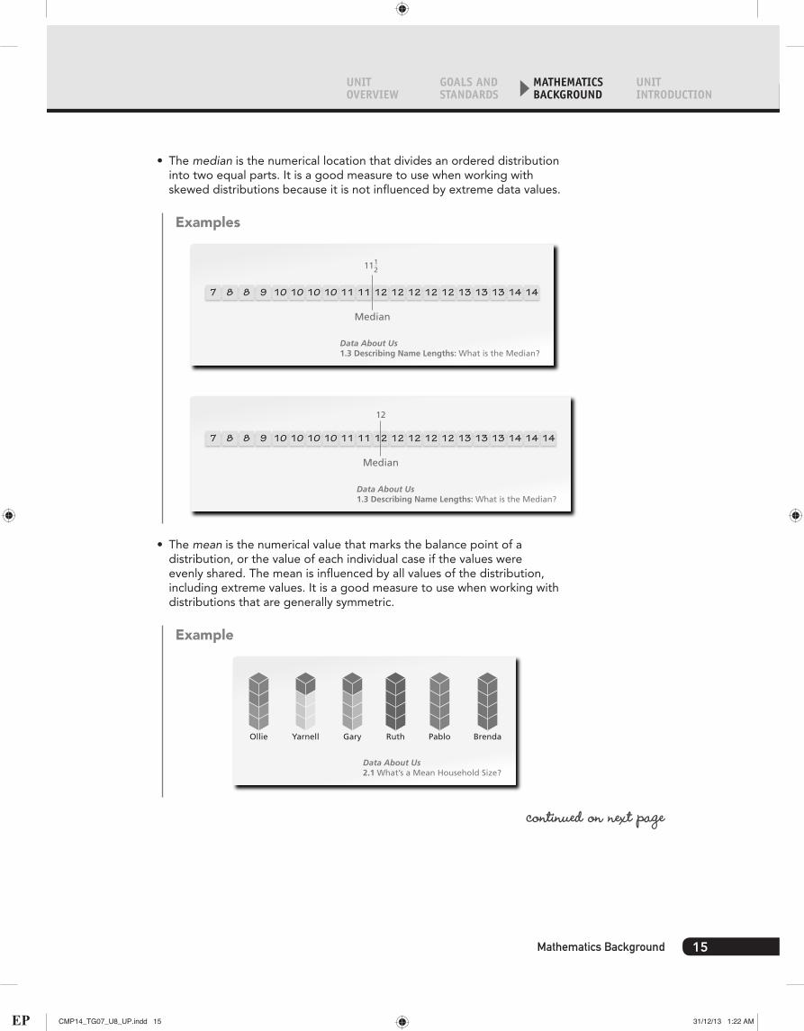
• The median is the numerical location that divides an ordered distribution into two equal parts. It is a good measure to use when working with skewed distributions because it is not influenced by extreme data values.
Examples
7 8 8 9 10 10 10 10 11 11 12 12 12 12 12 13 13 13 14 14
Median
1112
Data About Us1.3 Describing Name Lengths: What is the Median?
7 8 8 9 10 10 10 10 11 11 12 12 12 12 12 13 13 13 14 1414
Median
12
Data About Us1.3 Describing Name Lengths: What is the Median?
• The mean is the numerical value that marks the balance point of a distribution, or the value of each individual case if the values were evenly shared. The mean is influenced by all values of the distribution, including extreme values. It is a good measure to use when working with distributions that are generally symmetric.
Example
Ollie Yarnell Gary Ruth Pablo Brenda
Data About Us2.1 What’s a Mean Household Size?
continued on next page
15Mathematics Background
CMP14_TG07_U8_UP.indd 15 31/12/13 1:22 AM

Look for these icons that point to enhanced content in Teacher Place
• The mode is the most frequent value in a data set. In Samples and Populations, students will work with the mode on occasion, because it is the only measure of center that can be found for categorical data.
Example
2.4 Growing Samples: What Size Sample to Use?
Median Hours of Sleep6.0
� � � �
�����
�����
��
��
��
6.5 7.0 7.5 8.0 8.5 9.0 9.5 10.0
Samples of Size 5There can be anynumber of modes:no mode,1 mode,2 modes, etc.
8.0 and 8.5 occur themost frequently. 8.0and 8.5 are the modes.
Measures of SpreadVariability measures how close together or spread out a distribution of values is. Measures of spread describe the degree of variability of the data values and the data values’ deviations from, or differences from, the measures of center.
When students analyze the variability of a distribution, they consider the following.
• How alike or different are the data values from each other?
• Which data values occur more frequently or less frequently?
• How spread out or close together are the data values in relation to each other?
• How spread out or close together are the data values in relation to a measure of center?
Students in Grade 7 use three measures of spread to describe distributions of data, two of which are related to specific measures of center.
• The range is the difference between the maximum and the minimum data values. When considering the range, students can also describe where gaps exist or how the data cluster between the maximum and the minimum.
Samples and Populations Unit Planning16
Interactive ContentVideo
CMP14_TG07_U8_UP.indd 16 31/12/13 1:22 AM

UNIT OVERVIEW
GOALS AND STANDARDS
MATHEMATICS BACKGROUND
UNIT INTRODUCTION
Example
Investigation 3 ACE: Exercise 7
maximum value – minimum value = range17 – 9 = 8
10 2 3 4 5 6 7 8 9 1210 11 13 14 15 16 17 18Number of Letters
Name Lengths of U.S. Students
Mean = 12.43MAD = 1.83
• The interquartile range (IQR) is used in connection with the median. It is the range of the middle 50, of the ordered data values. It provides a numerical measure of how close or widely spread out the data values in the 2nd and 3rd quartiles of a distribution are from the median. The IQR is visually represented by the box of a box-and-whisker plot. The IQR also helps to identify outliers, data values that are unexpected compared to the other data values in a distribution.
Example
Investigation 1 ACE: Exercises 27–32
Q1 – Q3 = IQR173 – 113.5 = 59.5
Beats per Minute (bpm)
60 70 80 90 100 110 120 130 140 150 160 170 180 190
Exercise Heart Rate
continued on next page
17Mathematics Background
CMP14_TG07_U8_UP.indd 17 31/12/13 1:22 AM

Look for these icons that point to enhanced content in Teacher Place
• The mean absolute deviation (MAD) is used in connection with the mean. In some sets of data, data values are concentrated close to the mean. In other sets of data, the data values are more widely spread out. The MAD calculates the average distance between each data value and the mean in a distribution.
Example
• Find the difference of each data value and the mean.
• Add all the differences you found together.
• Divide that sum by the number of data values.
• The final quotient is the mean absolute deviation.
1510
5
56
1015
33
0
4012 16Number of Minutes
20 24 28 32 36
Scenic Trolley Wait Times
Data About Us3.3 Is It Worth the Wait? Determiningand Describing Variability Using the MAD
For all three measures of spread, the smaller the measure, the less variation of the data values; the larger the measure, the greater the variation of the data values. Smaller measures of spread indicate consistency, while larger measures of spread indicate inconsistency.
Exploring Variation
Variation refers to the similarities and differences found among data values in a distribution. When multiple samples are taken from one population, there is a natural variation that occurs. Data values vary within a single sample, and one sample of a population will vary from another sample of the same population. Understanding this variability is at the heart of understanding samples.
In Samples and Populations, students encounter the natural variation that occurs when studying different samples taken from the same population. Students will use statistics and data analysis to describe areas of stability (or consistency) in the natural variation of a distribution.
You can use questions such as the ones below to help students think about variation and stability.
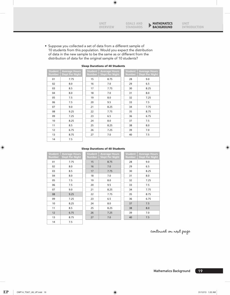
You analyze the distribution of a sample of 10 students’ sleep durations per night in order to draw conclusions about the sleep durations of a population of 40 students.
Samples and Populations Unit Planning18
Interactive ContentVideo
CMP14_TG07_U8_UP.indd 18 31/12/13 1:22 AM
UNIT OVERVIEW
GOALS AND STANDARDS
MATHEMATICS BACKGROUND
UNIT INTRODUCTION
• Suppose you collected a set of data from a different sample of 10 students from this population. Would you expect the distribution of data in the new sample to be the same as or different from the distribution of data for the original sample of 10 students?
StudentNumber
Average HoursSlept Per Night
01
02
03
04
05
06
07
08
09
10
11
12
13
14
7.75
8.0
8.5
8.0
7.5
7.5
9.0
9.25
7.25
8.25
8.5
6.75
8.75
7.5
StudentNumber
Average HoursSlept Per Night
15
16
17
18
19
20
21
22
23
24
25
26
27
8.75
7.0
7.75
7.0
8.0
9.5
8.25
7.75
6.5
8.0
8.25
7.25
7.0
StudentNumber
Average HoursSlept Per Night
28
29
30
31
32
33
34
35
36
37
38
39
40
9.0
6.5
8.25
8.0
7.25
7.5
7.75
8.75
6.75
7.5
8.0
7.0
7.5
Sleep Durations of 40 Students
StudentNumber
Average HoursSlept Per Night
StudentNumber
Average HoursSlept Per Night
28
29
30
31
32
33
34
35
36
37
38
39
40
9.0
6.5
8.25
8.0
7.25
7.5
7.75
8.75
6.75
7.5
8.0
7.0
7.5
Sleep Durations of 40 Students
15
16
17
18
19
20
21
22
23
24
25
26
27
8.75
7.0
7.75
7.0
8.0
9.5
8.25
7.75
6.5
8.0
8.25
7.25
7.0
01
02
03
04
05
06
07
08
09
10
11
12
13
14
7.75
8.0
8.5
8.0
7.5
7.5
9.0
9.25
7.25
8.25
8.5
6.75
8.75
7.5
Average HoursSlept Per Night
StudentNumber
continued on next page
19Mathematics Background
CMP14_TG07_U8_UP.indd 19 31/12/13 1:22 AM

Look for these icons that point to enhanced content in Teacher Place
StudentNumber
Average HoursSlept Per Night
Average HoursSlept Per Night
StudentNumber
Average HoursSlept Per Night
28
29
30
31
32
33
34
35
36
37
38
39
40
9.0
6.5
8.25
8.0
7.25
7.5
7.75
8.75
6.75
7.5
8.0
7.0
7.5
Sleep Durations of 40 Students
StudentNumber
15
16
17
18
19
20
21
22
23
24
25
26
27
8.75
7.0
7.75
7.0
8.0
9.5
8.25
7.75
6.5
8.0
8.25
7.25
7.0
01
02
03
04
05
06
07
08
09
10
11
12
13
14
7.75
8.0
8.5
8.0
7.5
7.5
9.0
9.25
7.25
8.25
8.5
6.75
8.75
7.5
• If you expect the distributions to be different, in what ways would the data be different (e.g., would there be differences among data values, locations of data values, measures of center or spread, or descriptions of shapes of distributions)?
6.0 6.5 7.0 7.5 8.0 8.5 9.0 9.5 10.0
Sleep Durations
(hours)
6.0 6.5 7.0 7.5 8.0 8.5 9.0 9.5 10.0
(hours)
Sleep Durations
Several questions may be used to highlight interesting aspects of variation.
•What does a distribution look like?
•How much do the data points vary from one another or from a measure of center?
In addition to these basic questions, students in Grade 7 begin to ask questions such as:
•Are there reasons why there is variation in these data?
•Are there reasons why two samples might vary from each other?
•Can you conclude anything about two samples, or about the population (or populations) from which they were drawn, by analyzing the difference between the two samples?
Samples and Populations Unit Planning20
Interactive ContentVideo
CMP14_TG07_U8_UP.indd 20 31/12/13 1:22 AM
UNIT OVERVIEW
GOALS AND STANDARDS
MATHEMATICS BACKGROUND
UNIT INTRODUCTION
Representing Data With Graphical Displays
Statisticians use data displays and statistics during the analysis part of the process of statistical investigation.
Students will construct and analyze graphs in Samples and Populations that they have already used a number of times during Grades K–6.
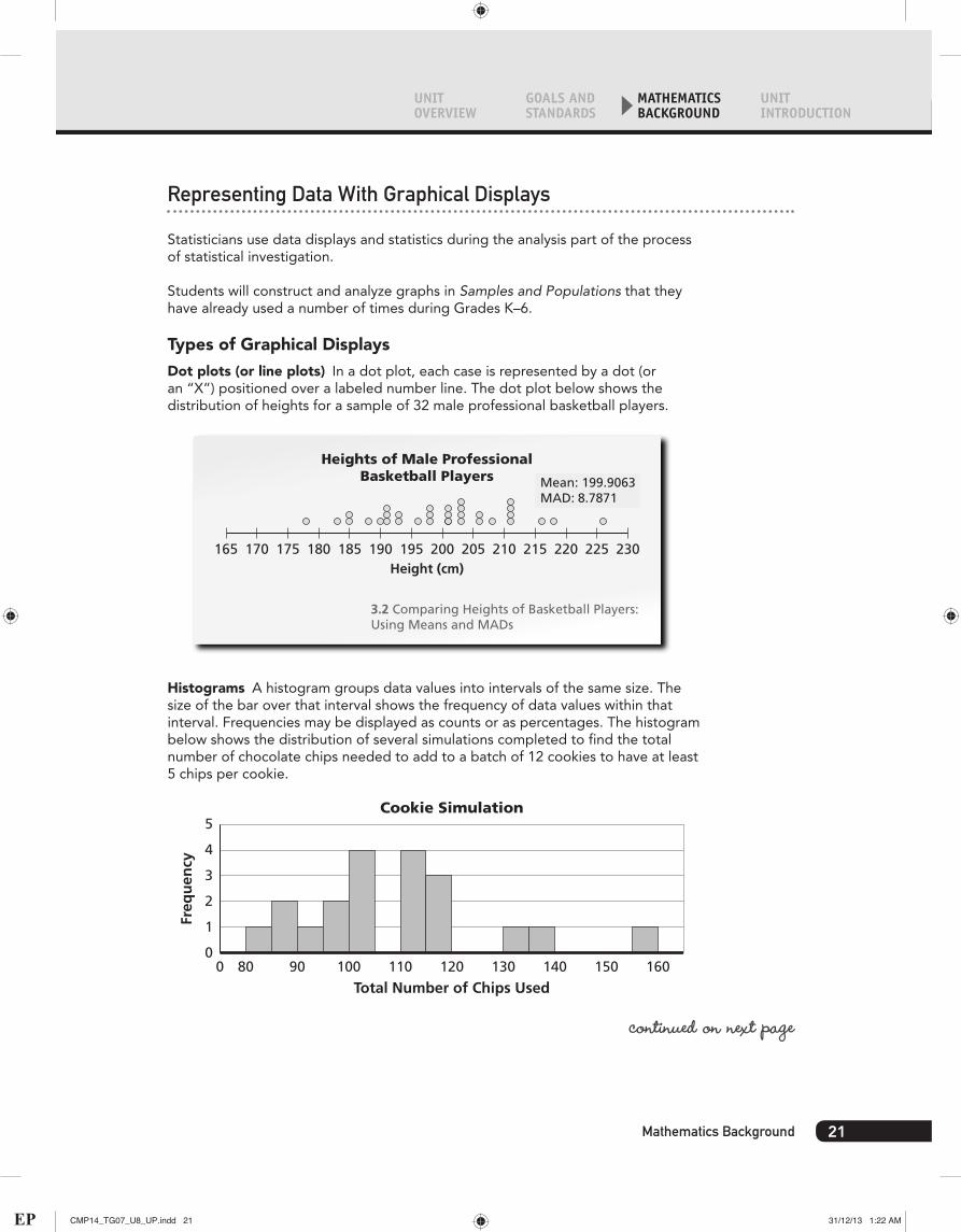
Types of Graphical DisplaysDot plots (or line plots) In a dot plot, each case is represented by a dot (or an “X”) positioned over a labeled number line. The dot plot below shows the distribution of heights for a sample of 32 male professional basketball players.
165 170 175 180 185 190 195 200 205 210 215 220 225 230
Heights of Male ProfessionalBasketball Players
Height (cm)
3.2 Comparing Heights of Basketball Players:Using Means and MADs
Mean: 199.9063MAD: 8.7871
Histograms A histogram groups data values into intervals of the same size. The size of the bar over that interval shows the frequency of data values within that interval. Frequencies may be displayed as counts or as percentages. The histogram below shows the distribution of several simulations completed to find the total number of chocolate chips needed to add to a batch of 12 cookies to have at least 5 chips per cookie.
Freq
uen
cy
1
00 80 90 100 110 120 130 140 150 160
2
3
4
5
Total Number of Chips Used
Cookie Simulation
continued on next page
21Mathematics Background
CMP14_TG07_U8_UP.indd 21 31/12/13 1:22 AM

Look for these icons that point to enhanced content in Teacher Place
Box-and-whisker plots Box plots are divided into quartiles and display properties of distributions, such as symmetry or skewness. The graphs below show the distributions of different size dog breeds; outliers and medians are marked.
Size
Midsize
Large
Small
10 12 14 16 18 20 22 24 26 28 302 4 6 8
Height (in.)
Heights of Dog Breeds
9
19
25
Reading Graphical DisplaysGraphs are a central component of data analysis and deserve special attention. There are three components of graph comprehension (Frances R. Curcio, Developing graph comprehension: elementary and middle school activities [Reston, VA: NCTM, 1989]).
165 170 175 180 185 190 195 200 205 210 215 220 225 230
Heights of Male ProfessionalBasketball Players
Height (cm)
3.2 Comparing Heights of Basketball Players:Using Means and MADs
Mean: 199.9063MAD: 8.7871
• Reading the data involves taking specific information from a graph to answer explicit questions. For example, how many male professional basketball players are 185 centimeters tall?
165 170 175 180 185 190 195 200 205 210 215 220 225 230
Heights of Male ProfessionalBasketball Players
Height (cm)
3.2 Comparing Heights of Basketball Players:Using Means and MADs
Two NBA players are185 centimeters tall.
Mean: 199.9063MAD: 8.7871
Samples and Populations Unit Planning22
Interactive ContentVideo
CMP14_TG07_U8_UP.indd 22 31/12/13 1:22 AM

UNIT OVERVIEW
GOALS AND STANDARDS
MATHEMATICS BACKGROUND
UNIT INTRODUCTION
• Reading between the data includes interpreting and integrating information presented in a graph. For example, what percent of heights for male professional basketball players are greater than the mean of 199.906 centimeters?
165 170 175 180 185 190 195 200 205 210 215 220 225 230
Heights of Male ProfessionalBasketball Players
Height (cm)
3.2 Comparing Heights of Basketball Players:Using Means and MADs
53% of the players aretaller than the mean of199.9063 centimeters.
Mean: 199.9063MAD: 8.7871
• Reading beyond the data involves extending, predicting, or inferring from data to answer implicit questions. For example, what is the typical height for male professional basketball players?
165 170 175 180 185 190 195 200 205 210 215 220 225 230
Heights of Male ProfessionalBasketball Players
Height (cm)
3.2 Comparing Heights of Basketball Players:Using Means and MADs
The typical height foran NBA player is199.9063 centimeters.
Mean: 199.9063MAD: 8.7871
Once students construct graphs, they use the graphs in the interpretation phase of the data-investigation process. This is when they need to ask questions about the graphs. The first two categories of questions—reading the data and reading between the data—are basic to understanding graphs. However, when students read beyond the data, they are exhibiting higher-order thinking skills, such as inference and justification.
23Mathematics Background
CMP14_TG07_U8_UP.indd 23 31/12/13 1:22 AM

Look for these icons that point to enhanced content in Teacher Place
Comparing Distributions
Students can compare two or more data sets with statistics. Students must sort out whether they are comparing data sets with equal numbers of data values (when counts can be used as frequencies) or data sets with unequal numbers of data values (when relative frequencies or percentiles need to be used).
Students often find it easier to start with data sets with equal numbers of data values and then move on to data sets with unequal numbers of data values. This progression helps students to more readily move from counts to percentiles, or relative frequencies. In Samples and Populations, most comparison work involves same-sized samples. There are good reasons for this. Students learn that statistics, such as the mean or median, drawn from samples of size 30 vary less than statistics drawn from samples of size 10. So, comparisons of samples are best when sample size is not another variable.
There are a few cases in which students compare unequal-sized data sets, primarily using box plots, a representation already organized using percentiles.
When comparing two or more data sets, the focus is on three features.
Center: Graphically, the center of a distribution is the point at which about half of the observations are on either side (median) or around which the distribution is balanced (mean). The two primary measures are the median and the mean for numerical data. These will have similar values for symmetric distributions, but the mean and median may be quite different for skewed distributions.
Example
The mean ofthe top dataset is 7.7. Themedian is 7.5.
The mean ofthe bottomdata set is7.675. Themedian is 7.5.
Comparing themeasures ofcenter, thesedata sets arevery similar.They have thesame medianand verysimilar means.
6.0 6.5 7.0 7.5 8.0 8.5 9.0 9.5 10.0
Sleep Durations
(hours)
6.0 6.5 7.0 7.5 8.0 8.5 9.0 9.5 10.0
(hours)
Samples and Populations Unit Planning24
Interactive ContentVideo
CMP14_TG07_U8_UP.indd 24 31/12/13 1:22 AM

UNIT OVERVIEW
GOALS AND STANDARDS
MATHEMATICS BACKGROUND
UNIT INTRODUCTION
Spread: The spread of a distribution refers to the variability of the data. If the observations cover a wide range, the spread is larger. If the observations are clustered around a single value, the spread is smaller. Three primary measures are the range, IQR (median), and MAD (mean).
Example
3.1 Solving an Archeological Mystery:Comparing Samples Using Box Plots
Site I
Site II
9 10 11 12 13 14 15 16 17 185 6 7 8
Neck Width (mm)
Site 1’s arrowhead neck widths aremuch more variable than Site II's.
The Site I data has a range of10 (18 – 8), while Site II only has arange of 5 (11 – 6).
Also, Site I’s IQR is 4 (15 – 11)while Site II's IQR is only 2 (9 – 7).
Shape: The shape of a distribution can be described as symmetrical or skewed. Shape also can be described by noticing number, size, and placement of gaps and clusters.
Example
Time (minutes)
Histogram E
44
2
4
6
046 48 50 52 54 56 58 60 62 64 66 68 70
Time (minutes)
Histogram F
44
2
4
6
046 48 50 52 54 56 58 60 62 64 66 68 70
Histogram F is fairlysymmetric but has nolarge clusters orgaps.
Histogram E isskewed to the leftand has a clusterfrom 56 minutes to64 minutes.
Data About UsLooking Back
continued on next page
25Mathematics Background
CMP14_TG07_U8_UP.indd 25 31/12/13 1:23 AM

Look for these icons that point to enhanced content in Teacher Place
Symmetry is an attribute used to describe the shape of a data distribution. When it is graphed, a symmetric distribution can be divided at the center so that each half is a mirror image of the other. A nonsymmetric distribution cannot.
When they are displayed graphically, some distributions of data have many more observations on one side of the graph than on the other. Distributions with data values clustered on the left and the tail extending to the right are said to be skewed right. Distributions with data values clustered on the right and the tail extending to the left are said to be skewed left.
The shape is symmetric.
The shape is skewed tothe left. Data are morespread out to the leftof the median.
The shape is skewed tothe right. Data are morespread out to the rightof the median.
4.2 Jumping Rope: Box-and-Whisker PlotsData About Us
0
5
140120100806040
10
15
20
25This histogram is skewed to the left.
0
10
6258545046
20
30
40
50
60This histogram is symmetric around the center.
Samples and Populations Unit Planning26
Interactive ContentVideo
CMP14_TG07_U8_UP.indd 26 31/12/13 1:23 AM

UNIT OVERVIEW
GOALS AND STANDARDS
MATHEMATICS BACKGROUND
UNIT INTRODUCTION
0
10
605040302010
20
30
40
50
60This histogram is skewed to the right.
Unexpected Features: Unexpected features may refer to gaps in the data (areas of the distribution where there are no observations) or the presence of outliers. An outlier is a value that one would not expect when examining the other values in a distribution. An extreme value is considered an outlier if it is at least 1.5 times the IQR less than the first quartile (Q1), or at least 1.5 times IQR greater than the third quartile (Q3). The box plot below shows two outliers. In addition, in some data situations, a data value being greater than 3 MADs less than or greater than the mean would be defined as an outlier.
0 5 10 15 20 25 30 35 40 45 50 55 60 65 70 75 80 85 90 95 100Top Speed (mi/h)
Wood-Frame Roller Coaster Speeds
Median
1.4 Are Steel-Frame Coasters Faster ThanWood-Frame Coasters? Using the IQR to Compare Samples
• 50 (Q1) – 15 = 35; there are two values (25 and 32) that are less than 35. These two values are outliers.
• 60 (Q3) + 15 = 75; no data values are above 75, so there are no outliers on the right-hand side of the box plot.
• The IQR is 10 (60 – 50)
• 1 × 10 (the IQR) = 1512
Sleep Last Night
2 2.5 3 3.5 4 4.5 5 5.5 6 6.5 7 7.5 8 8.5 9 9.5 10 10.5 11 11.5 12
Hours
Three values(5, 5.5, and 5.5)are outliers. Theyare outside ofthree MADs awayfrom the mean.
Three values (11.2,11.5, and 11.8) areoutliers. They areoutside of three MADsaway from the mean.
2.3 Choosing Random Samples: ComparingSamples Using Center and Spread
27Mathematics Background
CMP14_TG07_U8_UP.indd 27 31/12/13 1:23 AM

Look for these icons that point to enhanced content in Teacher Place
Variability Across Samples: Expected From Natural Variability or Due to Meaningful Differences Between Samples?
Variability is found in any set of data. Not all math test scores are the same, not all students watch the same number of hours of TV, and not all basketball players are the same heights. When students compare two sets of data, they should expect the distributions to be different. They need a way, however, to decide whether the differences are expected due to natural variability or to meaningful differences between samples.
For instance, in Problem 3.1, students compare box plots of six samples of arrowhead data. Looking at the two box plots below, you can see that the differences between the sample data from the Big Goose Creek site and Wortham Shelter site are fairly similar. They have a common attribute: they come from the same time period. Any differences in the samples of these two sites may simply be due to natural variability.
Length (mm)
Arrowheads
Site
10 15 20 25 30 35 40 45 50 55 60 65 70 75 80
Wortham Shelter
Big Goose Creek
On the other hand, consider the two dot plots below of male professional basketball player heights and female professional basketball player heights.
165 170 175 180 185 190 195 200 205 210 215 220 225 230
Heights of Male ProfessionalBasketball Players
Height (cm)
3.2 Comparing Heights of Basketball Players:Using Means and MADs
Mean: 199.9063MAD: 8.7871
Samples and Populations Unit Planning28
Interactive ContentVideo
CMP14_TG07_U8_UP.indd 28 31/12/13 1:23 AM
UNIT OVERVIEW
GOALS AND STANDARDS
MATHEMATICS BACKGROUND
UNIT INTRODUCTION
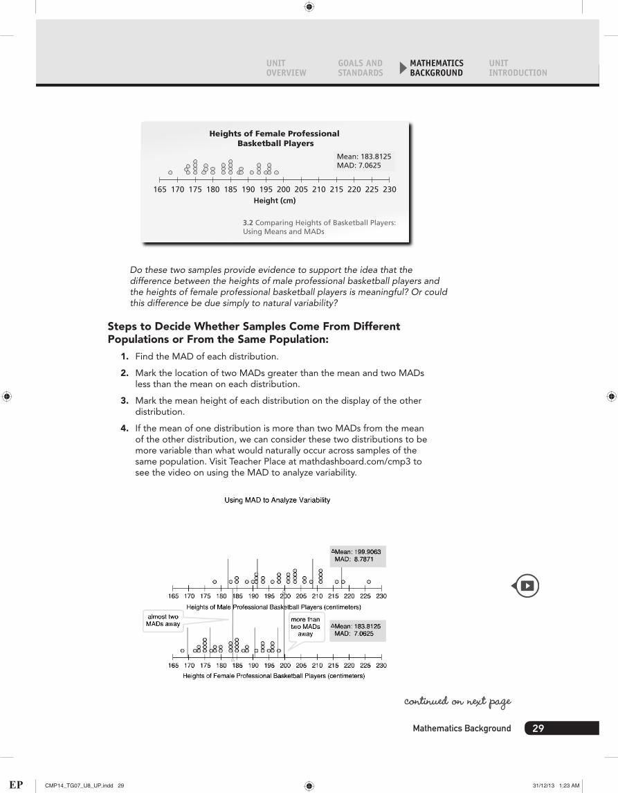
3.2 Comparing Heights of Basketball Players:Using Means and MADs
165 170 175 180 185 190 195 200 205 210 215 220 225 230
Heights of Female Professional Basketball Players
Height (cm)
Mean: 183.8125MAD: 7.0625
Do these two samples provide evidence to support the idea that the difference between the heights of male professional basketball players and the heights of female professional basketball players is meaningful? Or could this difference be due simply to natural variability?
Steps to Decide Whether Samples Come From Different Populations or From the Same Population:
1. Find the MAD of each distribution.
2. Mark the location of two MADs greater than the mean and two MADs less than the mean on each distribution.
3. Mark the mean height of each distribution on the display of the other distribution.
4. If the mean of one distribution is more than two MADs from the mean of the other distribution, we can consider these two distributions to be more variable than what would naturally occur across samples of the same population. Visit Teacher Place at mathdashboard.com/cmp3 to see the video on using the MAD to analyze variability.
continued on next page
29Mathematics Background
CMP14_TG07_U8_UP.indd 29 31/12/13 1:23 AM
Look for these icons that point to enhanced content in Teacher Place
While the two distributions in the animation above overlap in terms of spreads, the difference between the means is 16.047 cm. Additionally, as seen above, the mean height of each set of players is an unexpected value in the distribution of the other set of players. You can conclude, therefore, that there is a meaningful difference between the two distributions that is not due to natural variability. It is not likely that these two populations have similar distributions of heights.
Sampling Plans
A census takes information from the entire population. Generally, conducting a census is not possible or reasonable because of factors such as cost and the size of the population. Instead, sampling is used to gain information about a whole population by analyzing only a part of it.
RepresentativenessA central issue in sampling is the need for representative samples. This includes identifying a sampling plan that would result in as representative a sample as possible without concern for the effects of variability or size.
Students often have intuitive notions about representativeness. They can discuss ways in which certain samples may or may not be “fair,” or in more technical terms, may or may not represent characteristics of all the members of a population. The terms representative and bias will help students focus on whether they think data taken from a sample may be used to give a “fair” reflection of what is true about a population.
To ensure that samples are representative, or fair, statisticians try to use random sampling plans. Each person or object in the population needs to have an equally likely chance to be included as part of a sample.
The concept of randomness is not an easy one for many students to grasp. One context that may help students think about what it means to choose randomly is the draw-names-from-a-hat strategy. The random sampling plans encountered in this Unit may all be compared to the idea of writing each data value on an identical slip of paper, putting each piece of paper in a hat and mixing thoroughly, and then drawing out one or more slips of paper.
Random samples are not always representative of a population. All types of samples vary. Random samples, however, have two important characteristics:
• Random samples are free from bias.
• Random samples of a large enough size generally give good predictions about the populations from which they are drawn.
Samples and Populations Unit Planning30
Interactive ContentVideo
CMP14_TG07_U8_UP.indd 30 31/12/13 1:23 AM

UNIT OVERVIEW
GOALS AND STANDARDS
MATHEMATICS BACKGROUND
UNIT INTRODUCTION
Random Sampling PlansA number of strategies for selecting samples at random are mentioned in this Unit, such as using spinners, tossing number cubes, and generating lists of values using a calculator. These strategies rely on prior knowledge about probability that students bring to the Unit. There is an equally likely chance for any number to be generated by any spin, toss, or calculator key press. This number may be used to select a member of a population as part of a sample, which means there is an equally likely chance for any member of a population to be included in the sample. Visit Teacher Place at mathdashboard.com/cmp3 to see the video on Random Sampling.
Generating Samples From a CalculatorIf you use a calculator to generate random numbers, you will need to think about how random digits are generated on the calculators students are using. Most graphing calculators and many nongraphing calculators have a function for generating decimal numbers. The number of digits in each decimal may be specified (for example, .42 is a two-digit decimal). Students can treat the decimal numbers .00 to .99 as whole numbers for selecting students from the database, with .00 representing student 100, .01 representing student 1, .02 representing student 2, and so on. Some calculators have a random-integer generator. For these calculators, one or more numbers are entered as part of the command. The command consists of the maximum and minimum numbers with which you are working.
continued on next page
31Mathematics Background
CMP14_TG07_U8_UP.indd 31 31/12/13 1:23 AM

Look for these icons that point to enhanced content in Teacher Place
It is also important to check whether students’ calculators generate the same ordered set of random numbers each time the calculator is turned on. If so, the calculator uses a “seed value” that causes it to begin generating random numbers in a specific way. Consult the manual for each calculator to learn how to change the seed value so that each student can generate a different list of random numbers.
Other Sampling PlansIn addition to random sampling, students consider other types of sampling: convenience sampling, voluntary-response sampling, and systematic sampling. Samples selected using one of these three methods have a greater potential to be biased, or not representative, of the population from which they are drawn.
• convenience sampling: a sampling plan in which all of the participants are chosen because they are convenient
• systematic sampling: a sampling plan that chooses participants in a methodical or rule-based way
• voluntary-response sampling: a sampling plan in which the participants select themselves to be part of the sample
Type of Sampling Plan
Convenience Sampling
• surveying the people in your neighborhood• surveying the people who come through a register at the grocery store
• choosing Social Security Numbers at random by using a computer's random number generator• assigning each person at a school a student ID number and using a spinner to choose student ID numbers at random
• surveying every third household on your block• surveying every fourth person who comes into a bank.
• gathering information from callers who agree to answer survey questions at the end of a call• having a voluntary survey booth at a blood drive
Examples
Random Sampling
Systematic Sampling
Voluntary-ResponseSampling
Sampling Plans
Samples and Populations Unit Planning32
Interactive ContentVideo
CMP14_TG07_U8_UP.indd 32 31/12/13 1:23 AM

UNIT OVERVIEW
GOALS AND STANDARDS
MATHEMATICS BACKGROUND
UNIT INTRODUCTION
Sample SizesStudents should develop a sound, general sense about what makes a good sample size. As a rule of thumb, students should use samples with 30 data values. Even with good sampling strategies, summary statistics, such as means and medians, of the samples will vary.
The accuracy of a sample statistic as a predictor of the population statistic improves with the size of the sample. In Samples and Populations, Investigation 2, students demonstrate that samples of 30 generally have mean or median distributions that cluster fairly closely around the population mean or median. Sample sizes of 25 to 30 are appropriate for most of the contexts that students at this level encounter.
Sampling DistributionsA sampling distribution is a distribution of data values, each of which is a statistic drawn from a sample. For instance, suppose you collect a sample of size 10. You can find the mean of this sample. This mean is one data value in a sampling distribution.
Repeat the process. Find multiple samples of size 10, and find the mean of each. This distribution of means is called a sampling distribution of means. You can then investigate how much these means vary from each other. The same process can be done with medians.
Interesting concepts arise from studying sampling distributions. For example, the sampling distribution of means from samples of size 30 still shows variation, but it shows much less variation than the sampling distribution of means of samples of size 20, 10, and so on. Moreover, the greater the size of the sample, the more the sampling distribution of means clusters around the true mean of the population. A random sample of size 30 usually gives an accurate prediction of the mean of the population.
33Mathematics Background
CMP14_TG07_U8_UP.indd 33 31/12/13 1:23 AM