Solutions for Today | Options for Tomorrow

Handling Skewed Emission Distributions in Natural Gas Systems

LCA XVIII: September 26, 2018

James Littlefield, Dan Augustine, Selina Roman-White, Greg Cooney, and Timothy J. Skone, P.E.

2

DISCLAIMER"This report was prepared as an account of work sponsored by an agency of the United States Government. Neither the United States Government nor any agency thereof, nor any of their employees, makes any warranty, express or implied, or assumes any legal liability or responsibility for the accuracy, completeness, or usefulness of any information, apparatus, product, or process disclosed, or represents that its use would not infringe privately owned rights. Reference herein to any specific commercial product, process, or service by trade name, trademark, manufacturer, or otherwise does not necessarily constitute or imply its endorsement, recommendation, or favoring by the United States Government or any agency thereof. The views and opinions of authors expressed herein do not necessarily state or reflect those of the United States Government or any agency thereof."

AttributionKeyLogic Systems, Inc.’s contributions to this work were funded by the National Energy Technology Laboratory under the Mission Execution and Strategic Analysis contract (DE-FE0025912) for support services.

Disclaimer and Attribution

3

NETL’s Life Cycle Analysis (LCA) Program• Supports NETL and DOE Office of Fossil Energy• Supports inter- and intra-DOE initiatives• Conducts research to improve approaches to energy

analysis• Builds and maintains life cycle model and databases

Figure adapted from American Gas Association literature (AGA, 2014)

• Analyzes natural gas systems using a bottom-up, unit process perspective

4

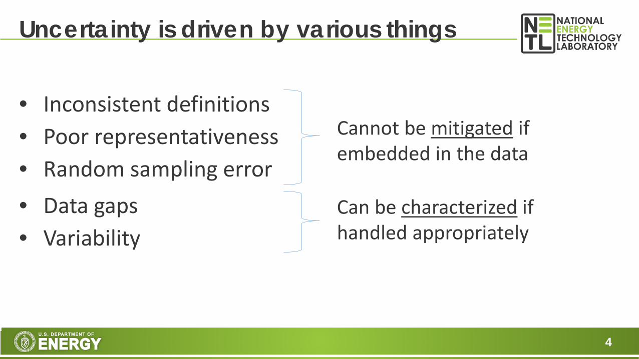
Uncertainty is driven by various things

• Inconsistent definitions• Poor representativeness• Random sampling error• Data gaps• Variability

Cannot be mitigated if embedded in the data

Can be characterized if handled appropriately

5

Deterministic modeling with selective scenarios

0

200

400

600

800

1,000

1,200

1,400N

GCC

NGC

C/CC

S

GTS

C

Flee

t

Coal

onl

y

10%

HP

10%

For

est R

esid

ue

Exist

ing

Gen

III+

Ons

hore

Con

vent

iona

l

Ons

hore

Adv

ance

d

Offs

hore

Gre

enfie

ld

Pow

er A

dditi

on

Upg

rade

Exist

ing

Geo

ther

mal

: Fla

sh S

team

Sola

r The

rmal

: Par

abol

ic T

roug

h

Natural Gas(2010 Domestic Mix)

Cofiring Nuclear Wind Conventional Hydropower

GHG

Em

issi

ons,

200

7 IP

CC 1

00-y

r GW

P(k

g CO

₂e/M

Wh)

RMA RMT ECF PT

Technology Assessment Compilation Report (2012)

• Deterministic modeling with scenarios that represent known constraints• Error bars represent extreme pairings of parameters and provide a bounding analysis

6

• Results do not include descriptive statistics• Overlap between scenarios implies equality, which hinders definitive conclusions

Deterministic modeling with possible outcomesLife Cycle GHG Footprint of a U.S. Energy Export Market for Coal and Natural Gas (2014)

0 400 800 1,200 1,600

Regional Coal

Russian NG (Yamal, RU to Shanghai, CN)

Regional LNG (Darwin, AU to Osaka, JP)

U.S. LNG (New Orleans, US to Shanghai, CN)

Regional Coal

Russian NG (Yamal, RU to Rotterdam, NL)

Regional LNG (Oran, DZ to Rotterdam, NL)

U.S. LNG (New Orleans, US to Rotterdam, NL)

Asia

Euro

pe

Greenhouse Gas Emissions AR5 20-yr GWP(kg CO₂e/MWh)

NG is 57% less to 13% greater than coal

NG is 57% less to 27% greater than coal

7

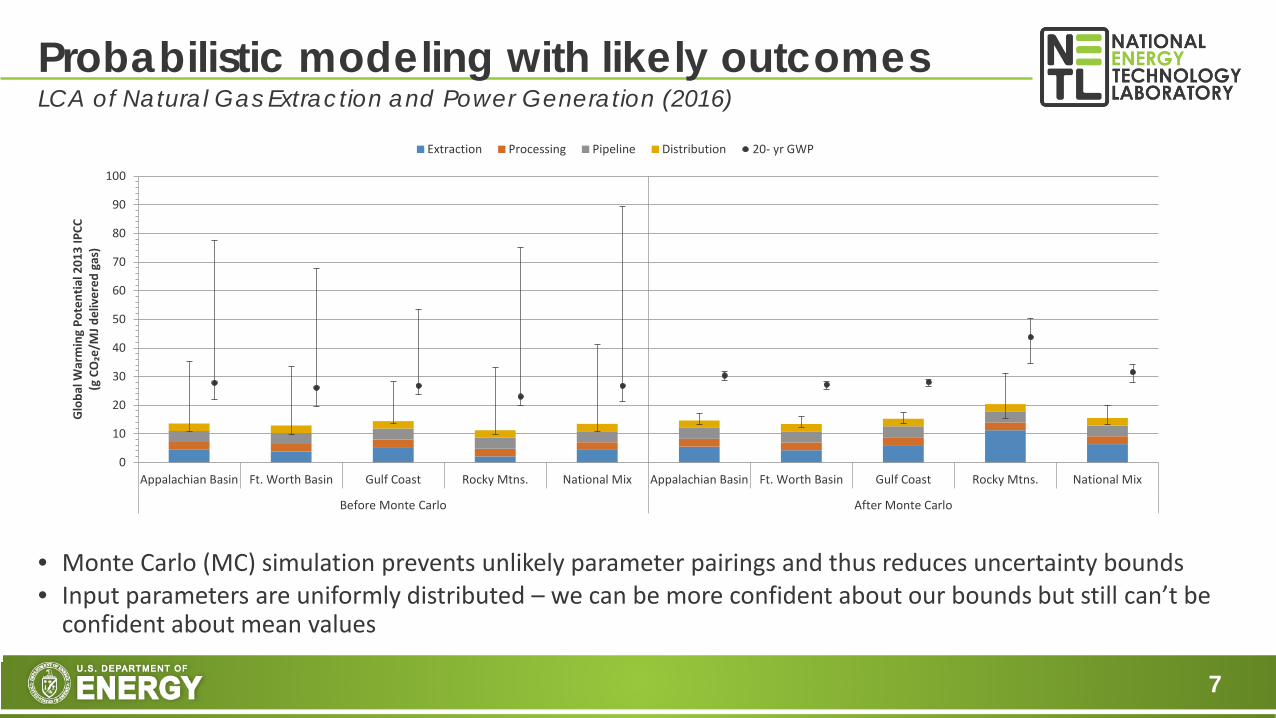
Probabilistic modeling with likely outcomes LCA of Natural Gas Extraction and Power Generation (2016)

0

10

20

30

40

50

60

70

80

90

100

Appalachian Basin Ft. Worth Basin Gulf Coast Rocky Mtns. National Mix Appalachian Basin Ft. Worth Basin Gulf Coast Rocky Mtns. National Mix

Before Monte Carlo After Monte Carlo

Glo

bal W

arm

ing

Pote

ntia

l 201

3 IP

CC(g

CO

₂e/M

J del

iver

ed g

as)

Extraction Processing Pipeline Distribution 20- yr GWP

• Monte Carlo (MC) simulation prevents unlikely parameter pairings and thus reduces uncertainty bounds• Input parameters are uniformly distributed – we can be more confident about our bounds but still can’t be

confident about mean values

8

Is Monte Carlo enough?

0

10

20

30

40

50

60

70

Freq

uenc

y

Transmission Equipment Leaks (count/facility-yr)

• Discarding outliers is not an option• Irregular distributions are prone to curve-fitting error• Lognormal distributions are infinitely long

Natural gas data are highly skewed…

9

Value of non-parametric bootstrapping

0

20

40

60

80

100

120

< 12.5 12.6 - 13.5 13.6 - 14.5 14.6 - 15.6 15.7 - 16.6 16.7 - 17.6 > 17.7

Freq

uenc

y

Transmission Equipment Leaks (count/facility-yr)

• Study objective: calculate average emissions, not likely emissions from a randomly selected well• Central limit theorem meets study objective without having a complete understanding of the data

Skewed, irregular distributions are resolved stochastically

10

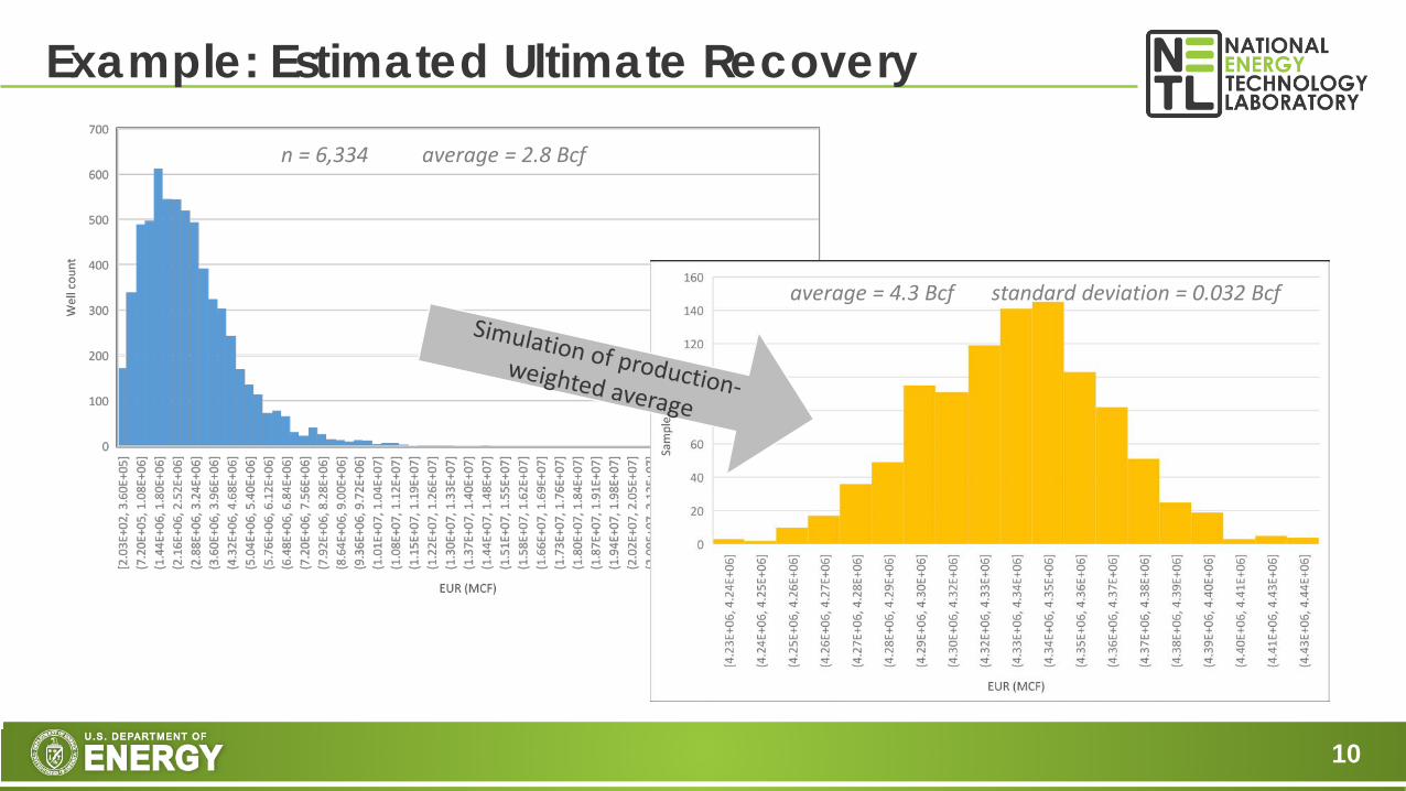
Example: Estimated Ultimate Recovery

n = 6,334 average = 2.8 Bcf

average = 4.3 Bcf standard deviation = 0.032 Bcf

11

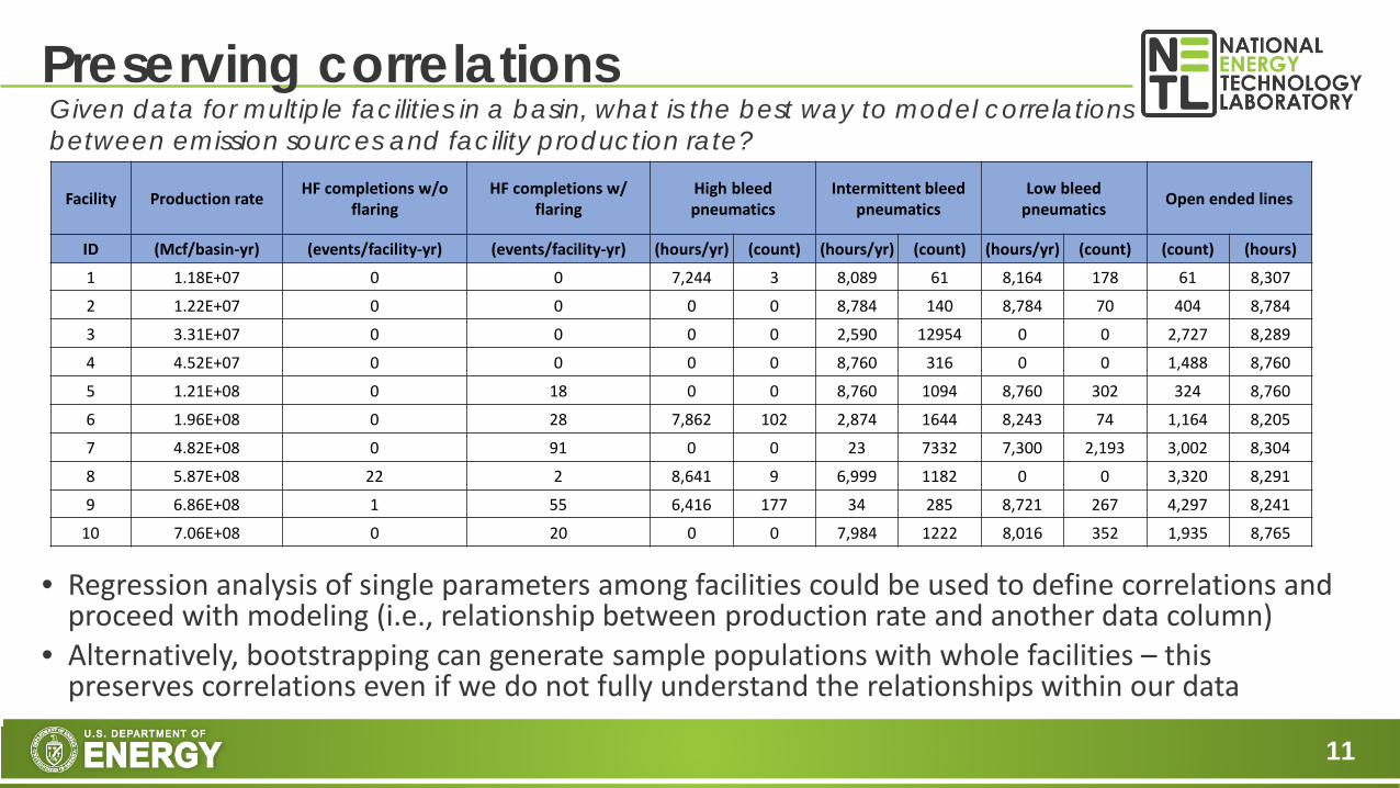
Preserving correlations

• Regression analysis of single parameters among facilities could be used to define correlations and proceed with modeling (i.e., relationship between production rate and another data column)

• Alternatively, bootstrapping can generate sample populations with whole facilities – this preserves correlations even if we do not fully understand the relationships within our data

Facility Production rate HF completions w/o flaring

HF completions w/ flaring

High bleed pneumatics

Intermittent bleed pneumatics

Low bleed pneumatics Open ended lines

ID (Mcf/basin-yr) (events/facility-yr) (events/facility-yr) (hours/yr) (count) (hours/yr) (count) (hours/yr) (count) (count) (hours)

1 1.18E+07 0 0 7,244 3 8,089 61 8,164 178 61 8,307

2 1.22E+07 0 0 0 0 8,784 140 8,784 70 404 8,784

3 3.31E+07 0 0 0 0 2,590 12954 0 0 2,727 8,289

4 4.52E+07 0 0 0 0 8,760 316 0 0 1,488 8,760

5 1.21E+08 0 18 0 0 8,760 1094 8,760 302 324 8,760

6 1.96E+08 0 28 7,862 102 2,874 1644 8,243 74 1,164 8,205

7 4.82E+08 0 91 0 0 23 7332 7,300 2,193 3,002 8,304

8 5.87E+08 22 2 8,641 9 6,999 1182 0 0 3,320 8,291

9 6.86E+08 1 55 6,416 177 34 285 8,721 267 4,297 8,241

10 7.06E+08 0 20 0 0 7,984 1222 8,016 352 1,935 8,765

Given data for multiple facilities in a basin, what is the best way to model correlations between emission sources and facility production rate?

12

0.00%

0.20%

0.40%

0.60%

0.80%

1.00%

1.20%

1.40%

0.00%

0.20%

0.40%

0.60%

0.80%

1.00%

1.20%

1.40%

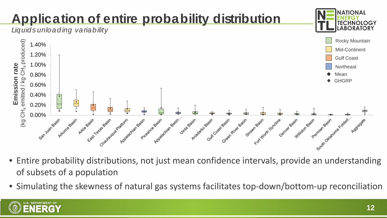
Application of entire probability distributionLiquids unloading variability

Emis

sion

rate

(k

g C

H4

emitt

ed /

kg C

H4

prod

uced

) Rocky Mountain

Mid-Continent

Gulf Coast

NortheastMeanGHGRP

• Entire probability distributions, not just mean confidence intervals, provide an understanding of subsets of a population

• Simulating the skewness of natural gas systems facilitates top-down/bottom-up reconciliation

13

• Deterministic comparisons are effective, until scenarios become too similar or error bounds overlap

• Stochastic methods allow us to represent likely uncertainty ranges, instead of possible uncertainty ranges

• Non-parametric bootstrapping simplifies highly variable, irregular distributions

• No single method is appropriate for all studies

Key TakeawaysParameterize with purpose and match methods to study objectives

14

Contact Information

Timothy J. Skone, P.E.Senior Environmental Engineer • U.S. DOE, NETL(412) 386-4495 • timothy.skone@netl.doe.gov

Greg CooneySenior Engineer • KeyLogicgregory.cooney@netl.doe.gov

James LittlefieldSenior Engineer • KeyLogicjames.littlefield@netl.doe.gov

netl.doe.gov/LCA LCA@netl.doe.gov @NETL_News