the potential impact of hydrodynamic leveling on the
TRANSCRIPT
Journal of Geodesy (2021) 95:90https://doi.org/10.1007/s00190-021-01543-3
ORIG INAL ART ICLE
The potential impact of hydrodynamic leveling on the quality of theEuropean vertical reference frame
Y. Afrasteh1 · D. C. Slobbe1 ·M. Verlaan2 ·M. Sacher3 · R. Klees1 · H. Guarneri1 · L. Keyzer1 · J. Pietrzak1 ·M. Snellen1 · F. Zijl2
Received: 29 October 2020 / Accepted: 9 July 2021 / Published online: 24 July 2021© The Author(s) 2021
AbstractThe first objective of this paper is to assess by means of geodetic network analyses the impact of adding model-basedhydrodynamic leveling data to the Unified European Leveling Network (UELN) data on the precision and reliability of theEuropean Vertical Reference Frame (EVRF). In doing so, we used variance information from the latest UELN adjustment. Themodel-based hydrodynamic leveling data are assumed to be obtained from not-yet existing hydrodynamic models coveringeither all European seas surrounding the European mainland or parts of it that provide the required mean water level withuniform precision. A heuristic search algorithm was implemented to identify the set of hydrodynamic leveling connectionsthat provide the lowest median of the propagated height standard deviations. In the scenario in which we only allow forconnections between tide gauges located in the same sea basin, all having a precision of 3 cm, the median of the propagatedheight standard deviations improved by 38% compared to the spirit leveling-only solution. Except for the countries around theBlack Sea, coastal countries benefit themost with amaximum improvement of 60% for Great Britain.We also found decreasedredundancy numbers for the observations in the coastal areas and over the entire Great Britain. Allowing for connectionsbetween tide gauges among all European seas increased the impact to 42%. Lowering the precision of the hydrodynamicleveling data lowers the impact. The results show, however, that even in case the assumed precision is 5 cm, the overallimprovement is still 29%. The second objective is to identify which tide gauges are most profitable in terms of impact. Ourresults show that these are the ones located in Sweden in which most height markers are located. The impact, however, hardlydepends on the geographic location of the tide gauges within a country.
Keywords Tide gauge · Quality · Hydrodynamic leveling · Network
1 Introduction
The assimilation of total water levels measured by tidegauges into a hydrodynamic model requires that both thehydrodynamic model and the observed water levels refer tothe same vertical datum. Total water level refers to the actuallevel of the water (with respect to a well-defined reference),which primarily varies due to tides, winds, and baroclinic
B Y. [email protected]
1 Delft University of Technology, Stevinweg 1, 2628 CN Delft,The Netherlands
2 Deltares, Boussinesqweg 1, 2629 HV Delft, The Netherlands
3 Federal Agency for Cartography and Geodesy,Richard-Strauss-Allee 11, 60598 Frankfurt am Main,Germany
effects (i.e., variations inwater density). Since hydrodynamicmodel domains typically do not stop at national boundaries,themodelers are suddenly confrontedwith the need for a uni-fied height datum. To fit their needs, this unified height datumshould be (i) accessible at islands and offshore platformsinside the model domain where tide gauges are available and(ii) highly accurate; we expect the standard deviation to be inthe order of 1 cm. The reason for the latter is that even smallerroneous tilts in the vertical reference surface may inducelarge water fluxes, which are a potential source of modelinstabilities. These requirements pose even in well-surveyedareas with a good geodetic infrastructure a tremendous chal-lenge for existing methods to realize a unified height datum.
Our area of interest serves in this respect as an illustra-tive example. The domain of the hydrodynamic model weare developing (i.e., the 3D DCSM-FM (Zijl et al. 2020))with the aim to forecast total water levels in the southern
123
90 Page 2 of 18 Y. Afrasteh et al.
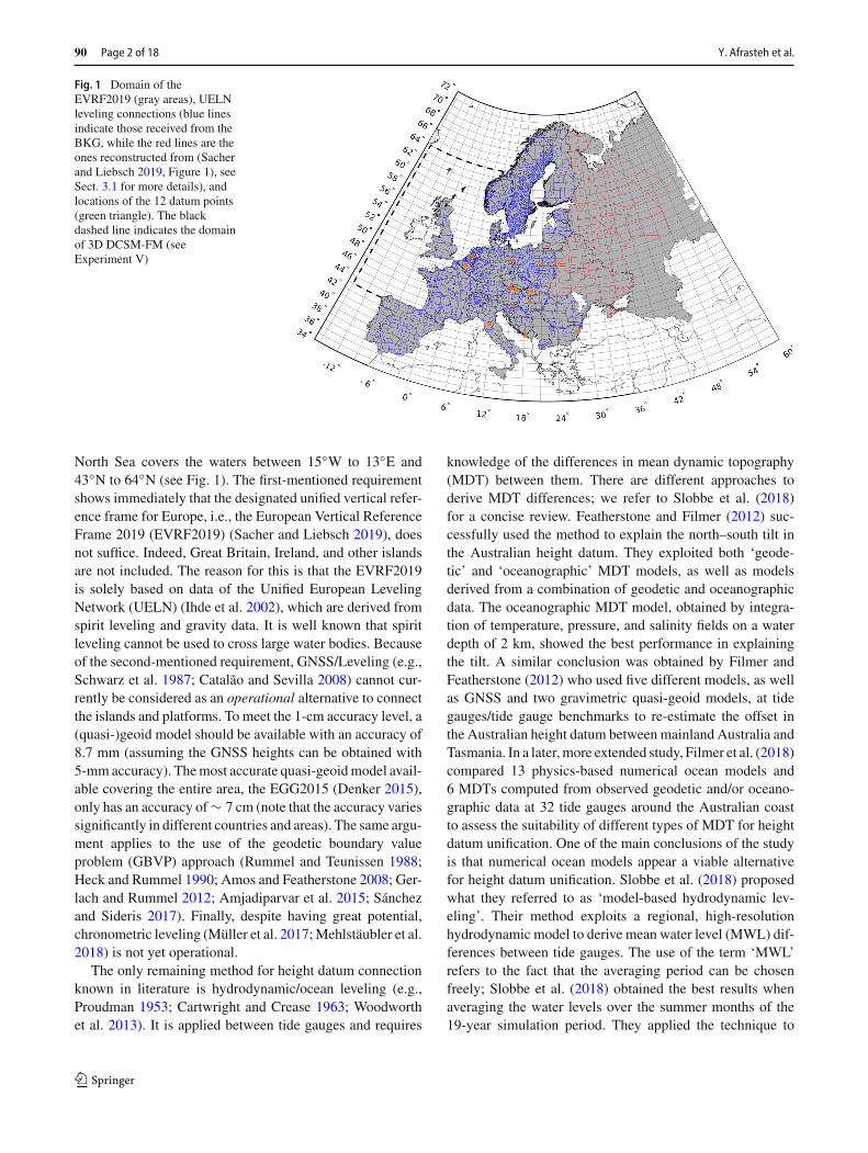
Fig. 1 Domain of theEVRF2019 (gray areas), UELNleveling connections (blue linesindicate those received from theBKG, while the red lines are theones reconstructed from (Sacherand Liebsch 2019, Figure 1), seeSect. 3.1 for more details), andlocations of the 12 datum points(green triangle). The blackdashed line indicates the domainof 3D DCSM-FM (seeExperiment V)
North Sea covers the waters between 15◦W to 13◦E and43◦N to 64◦N (see Fig. 1). The first-mentioned requirementshows immediately that the designated unified vertical refer-ence frame for Europe, i.e., the European Vertical ReferenceFrame 2019 (EVRF2019) (Sacher and Liebsch 2019), doesnot suffice. Indeed, Great Britain, Ireland, and other islandsare not included. The reason for this is that the EVRF2019is solely based on data of the Unified European LevelingNetwork (UELN) (Ihde et al. 2002), which are derived fromspirit leveling and gravity data. It is well known that spiritleveling cannot be used to cross large water bodies. Becauseof the second-mentioned requirement, GNSS/Leveling (e.g.,Schwarz et al. 1987; Catalão and Sevilla 2008) cannot cur-rently be considered as an operational alternative to connectthe islands and platforms. To meet the 1-cm accuracy level, a(quasi-)geoid model should be available with an accuracy of8.7 mm (assuming the GNSS heights can be obtained with5-mmaccuracy). Themost accurate quasi-geoidmodel avail-able covering the entire area, the EGG2015 (Denker 2015),only has an accuracy of∼ 7 cm (note that the accuracy variessignificantly in different countries and areas). The same argu-ment applies to the use of the geodetic boundary valueproblem (GBVP) approach (Rummel and Teunissen 1988;Heck and Rummel 1990; Amos and Featherstone 2008; Ger-lach and Rummel 2012; Amjadiparvar et al. 2015; Sánchezand Sideris 2017). Finally, despite having great potential,chronometric leveling (Müller et al. 2017;Mehlstäubler et al.2018) is not yet operational.
The only remaining method for height datum connectionknown in literature is hydrodynamic/ocean leveling (e.g.,Proudman 1953; Cartwright and Crease 1963; Woodworthet al. 2013). It is applied between tide gauges and requires
knowledge of the differences in mean dynamic topography(MDT) between them. There are different approaches toderive MDT differences; we refer to Slobbe et al. (2018)for a concise review. Featherstone and Filmer (2012) suc-cessfully used the method to explain the north–south tilt inthe Australian height datum. They exploited both ‘geode-tic’ and ‘oceanographic’ MDT models, as well as modelsderived from a combination of geodetic and oceanographicdata. The oceanographic MDT model, obtained by integra-tion of temperature, pressure, and salinity fields on a waterdepth of 2 km, showed the best performance in explainingthe tilt. A similar conclusion was obtained by Filmer andFeatherstone (2012) who used five different models, as wellas GNSS and two gravimetric quasi-geoid models, at tidegauges/tide gauge benchmarks to re-estimate the offset inthe Australian height datum between mainland Australia andTasmania. In a later,more extended study, Filmer et al. (2018)compared 13 physics-based numerical ocean models and6 MDTs computed from observed geodetic and/or oceano-graphic data at 32 tide gauges around the Australian coastto assess the suitability of different types of MDT for heightdatum unification. One of the main conclusions of the studyis that numerical ocean models appear a viable alternativefor height datum unification. Slobbe et al. (2018) proposedwhat they referred to as ‘model-based hydrodynamic lev-eling’. Their method exploits a regional, high-resolutionhydrodynamic model to derive mean water level (MWL) dif-ferences between tide gauges. The use of the term ‘MWL’refers to the fact that the averaging period can be chosenfreely; Slobbe et al. (2018) obtained the best results whenaveraging the water levels over the summer months of the19-year simulation period. They applied the technique to
123
The potential impact of hydrodynamic leveling on the quality of the European vertical... Page 3 of 18 90
transfer Amsterdam ordnance datum (Normaal AmsterdamsPeil, NAP) from the Dutch mainland to the Dutch Waddenislands. Based on a high-resolution 2Dhydrodynamicmodel,extended to account for depth-averaged water density vari-ations, Slobbe et al. (2018) showed that for each Waddenisland several connections are available that allow to transferNAP with (sub-)centimeter accuracy.
In view of the above-formulated requirements for a uni-fied height datum that meets the needs of the hydrodynamicmodelers, we believe that for our area of interest hydrody-namic/ocean leveling has great potential. In particular, theimplementation which exploits a numerical model. The rea-sons are threefold. First, because themethod indeed allows totransfer the height datum to all tide gauges inside the modeldomain. Second, because it is potentially accurate. Third,because a rigorous implementation (i.e., one that exploitsa hydrodynamic model that resolves all relevant 3D physi-cal processes) of the method is realizable in the short term.The second reason is suggested by the results obtained byWoodworth et al. (2013), Filmer et al. (2018), Slobbe et al.(2018). Despite the fact that the numerical models used inthese studies lacked spatial/temporal resolution and/or didnot account for all relevant 3D physical processes [(Wood-worth et al. 2013, Section 7.2) and (Slobbe et al. 2018,Section 5)], their performance was good in comparison withthe results obtained with alternative methods. Moreover, theuse of numerical models provides the freedom to choosethe averaging period. This allows to avoid, for example, thestorm periods. Regarding the last reason, indeed, many mod-els have been developed (see https://eurogoos.eu/models/ foran overview) although for different applications. Many ofthese are incomplete in terms of physics and/or lack of res-olution. As such, they are not suitable for our purpose. Atthe same time, however, we can highlight that all key build-ing blocks to design a model that resolves all relevant 3Dphysical processes are available. This applies not only to ourarea of interest, but in fact to almost all European waters.These building blocks include parallel software packagesthat can handle unstructured meshes needed to run large,high-resolutionmodels (e.g., Deltares 2021), high-resolutionmeteorological forcing reanalysis datasets (e.g., Hersbachet al. 2020), river discharge data (e.g., Donnelly et al. 2015;Wilkinson et al. 2014), and a high-resolution bathymetry(e.g., EMODnet Bathymetry Consortium 2018).
Indeed, to connect all tide gauges within the domain ofour hydrodynamic model we could follow the approach bySlobbe et al. (2018). That is, we connect all tide gauges tothe NAP. This approach, however, requires a model that hasa good performance at all tide gauge locations even thoughsome are at the same mainland and can be connected byspirit leveling. Apart from that, all errors in the vertical ref-erence of the involved Dutch tide gauge(s) propagate one toone to the vertical reference of the tide gauges of interest.
Because the former involves great efforts to achieve it andthe latter is not desirable, we propose combining ‘hydro-dynamic leveling data’ with the UELN data and use thecombined dataset to compute a new realization of the EVRSthat covers our whole domain of interest. This proposal is,indeed, a bit similar to what is advocated by Filmer et al.(2014). To maximize the network strength, we advocate toestablish hydrodynamic leveling connections in all Europeanwaters. This, of course, requires a model covering all Euro-peanwaters or a set ofmodels that each cover a separate basin.With hydrodynamic leveling connections, we mean connec-tions between tide gauge benchmarks that can be establishedby using the observation-derivedMWLs relativewith respectto the tide gauge benchmarks and the model-derived MWLdifferences between tide gauges. Note that here the model-derived MWL differences are obtained from models that donot assimilate geodetic information. The pursued strategyalso benefits other users of the EVRF as we may expect thatcombining both datasets improves the quality of the levelingnetwork and hence the derived VRF. In particular, addinghydrodynamic leveling data helps to detect/suppress system-atic errors that spirit leveling is susceptible to (e.g., Pennaet al. 2013).
The aim of this paper is twofold. First, to assess the impactof adding model-based hydrodynamic leveling connectionsto the UELN dataset on the quality of the EVRF. Second, toassess which connections, and hence tide gauges, are mostprofitable in terms of impact when realizing the EVRS. Thesecond objective is motivated by the fact that in Europe thereare many tide gauges. Not all of them can be used to establishhydrodynamic leveling connections. Indeed, a prerequisite isthat the benchmarks of the tide gauges located on the Euro-pean mainland are connected to the UELN. However, evenif this requirement is met, the location might be unsuitableif the local water levels are not resolved by the hydrody-namic model. The question, however, can also be turnedaround: which hydrodynamic leveling connections do havethe largest impact on the quality of the VRF? The answerto this question provides guidance where to focus in thedevelopment/calibration of the hydrodynamic model(s). Toachieve our objectives, we conducted several geodetic net-work analyses using different scenarios. For the UELN data,we relied on variance information from the latest UELNadjustment. The required MWL differences between tidegauges are assumed to have a uniform precision and areassumed to be obtained from not-yet existing hydrodynamicmodels (see above) covering all European Seas surroundingthe European mainland or parts of it. Indeed, the full poten-tial of hydrodynamic leveling is exploited when we haveone large model that allows to establish long-distance con-nections. In terms of model development, a more plausiblescenario is to start with models covering separate sea basins(e.g., the Mediterranean Sea). This implies that we can only
123
90 Page 4 of 18 Y. Afrasteh et al.
establish connections between tide gauges within the samesea basin.
The paper is organized as follows: Section 2 describes theheight network adjustment, the way the impact of addinghydrodynamic leveling data is assessed, and the methodused to determine which hydrodynamic leveling connectionsare actually added. Section 3 introduces the datasets usedthroughout this paper. Section 4 introduces the setup of theexperiments conducted in this study. The results of the exper-iments are presented and discussed in Sect. 5. Finally, weconclude by emphasizing the main findings and identifyingtopics for future research.
2 Methodology
2.1 Height network adjustment
The height network adjustment is conducted using weightedleast squares. For the two observation groups (i.e., the spiritand hydrodynamic leveling data), the Gauss–Markov modeltakes the form
y = Ax + e, (1)
where
y =(yslyhl
), A =
(Asl
Ahl
), and e =
(eslehl
). (2)
y is the observation vector, A is the design matrix, x is thevector of unknown parameters, e is the vector of residuals,and subscripts sl and hl stand for spirit leveling and hydro-dynamic leveling, respectively. The stochastic properties ofthe residuals are described by
E{e} = 0, D{e} = Qy =(Qsl 00 Qhl
), (3)
where E{.} denotes the statistical expectation operator, D{.}is the dispersion operator, Qy is the combined variance-co-variance matrix of the two observations groups, Qsl is thevariance-covariance matrix of the spirit leveling dataset, andQhl is the full variance-covariance matrix of the hydrody-namic leveling dataset. Qhl is obtained by error propagation,assuming a uniform precision for the difference betweenthe observation- and model-derived MWLs at a tide gaugelocation (where the observation-derived MWL is expressedrelative to the tide gauge bench mark). That is,
Qhl = AhlQdMWLAThl, (4)
where QdMWL is the diagonal variance-covariance matrix ofthe differences between the observation- and model-derived
MWLs at the tide gauge locations and Ahl is the designmatrix of the hydrodynamic leveling dataset. We assume thatthe contribution of the observation-derivedMWLs expressedrelative with respect to the tide gauge benchmarks to theerror budget of the hydrodynamic leveling data is negligible.According to us, this is justified for the following reason.Today’s instantaneous water levels are measured with a stan-dard deviation of a few centimeters, which implies that thestandard deviation of the mean is already at the sub-mm levelfor one month of data. Moreover, the connection betweenthe tide gauge zero and the tide gauge benchmark can easilybe determined using first-order leveling with sub-mm accu-racy too. Regarding the contribution of the model-derivedMWLs, we currently lack a proper stochastic model. It isexpected that some degree of spatial correlation exists andthat the accuracy will vary somewhat from location to loca-tion. The determination of a proper stochastic model willbe the subject of a future study. Here we will use the mostsimple model possible, namely the model which assumesuniform and uncorrelated noise. Note, anyway, that contraryto spirit leveling, the uncertainty of hydrodynamic levelingdata is likely independent of the distance between the twoinvolved tide gauges. In fact, the noise level mainly dependson the ability of the hydrodynamic model to represent thelocal MWL.
In realizing the EVRF2019, the datum defect is solved byadding the minimal constraint that for 12 datum points (seeFig. 1) the sum of the height changes is zero. The drawbackof using this constraint is that the propagated standard devi-ations of the adjusted heights depend on the height marker(also referred to as “height benchmark” or “leveling bench-mark”) distance to the datum points (Sacher and Liebsch2019). To assess the impact of adding hydrodynamic level-ing data on the quality of the leveling network, we conductedan experiment in which we used the constraint that the sumof height changes of all height markers is zero (Teunissen2006). This form ofminimal constraint adjustment, known asinner constraint adjustment, provides similar results as usingthe pseudo-inverse in the least-squares adjustment (Ogun-dare 2018). Indeed, to realize the EVRS the use of the innerconstraint adjustment is not a proper alternative to solve thedatum defect as also benchmarks in geodynamically unstableregions will affect the datum.
2.2 Assessing the impact of adding hydrodynamicleveling data
In general, the quality of a geodetic network can be char-acterized by (i) precision, (ii) reliability, and (iii) cost(Amiri-Simkooei et al. 2012). In this paper, we focus onthe first two criteria. The precision of a geodetic network isdescribed by the variance-covariance matrix of the estimated
123
The potential impact of hydrodynamic leveling on the quality of the European vertical... Page 5 of 18 90
parameters Qx̂ , with
Qx̂ =(ATQ−1
y A)−1
. (5)
In reporting the precision, we focus on the propagated stan-dard deviations (SDs) of the adjusted heights (i.e., the squareroot of the diagonal elements of Qx̂ ); themedian of this valuefor all height markers of the network, as well as the medianvalue per country. The median value for all height markersof the network is also used to determine which hydrody-namic leveling connections will be added to the network (seeSect. 2.3). Note that we use the median because the propa-gated height SDs for all height markers are not normallydistributed.
The reliability of a geodetic network refers to its abil-ity to detect and resist against outliers in the observations(Seemkooei 2001a).We study the impact on the reliability byanalyzing the redundancy numbers (see Seemkooei 2001b).The redundancy numbers are the diagonal elements of theso-called redundancy matrix R defined as
R = I − A(ATQ−1
y A)−1
ATQ−1y , (6)
where I is the identity matrix. Redundancy numbers expresshow the redundancy is distributed over the observations. Assuch, they depend on the configuration of the network andhow well the height markers are connected to each other.For uncorrelated measurements, their value ranges between0 and 1. The smaller/larger its value, the larger/smaller themagnitude of the outlier that can be detected as well as itsinfluence on the estimated parameters. It is desirable to havea networkwith relatively large and uniform redundancy num-bers, so that the ability to detect outliers is the same in everypart of the network (Baarda 1968). Similar to the way weanalyze the impact on precision, we will also report changesin the median value of the redundancy numbers for the entirenetwork and per country.
2.3 Choice of the hydrodynamic levelingconnections
Given N tide gauges, maximum N − 1 independent hydro-dynamic leveling connections can be established. By inde-pendent, we mean the connections that do not form anyclosed circuit. Indeed, the model-derived MWL differencesbetween the tide gauges are obtained from the MWLs atthe tide gauges. As such, adding a connection that closesa circuit does not add any new information and resultsthe full variance-covariance matrix obtained using Eq. 4 tobecome singular. The number of possible connections canbe extremely large. Considering N tide gauges, the numberof possibilities to establish N − 1 independent connections
among them equals K = NN−2 (Cayley’s formula (Aignerand Ziegler 1998)). Europe has a relatively dense networkof tide gauges that contains hundreds of stations. Assuming200 out of them can be used to establish hydrodynamic lev-eling connections, K equals 200198. To evaluate which set ofconnections has the largest impact, i.e. results in the lowestmedian SD of the adjusted heights, K least-squares solutionshave to be computed. Despite the fact that the computationalload can be reduced significantly by exploiting the recursiveleast-squares method (Teunissen 2006) and only computingthe diagonal elements of the variance-covariance matrix ofthe estimated unknowns, still evaluating all K solutions isnot feasible.
Therefore, we use a heuristic searchmethod that identifiesthe connections one by one. In each step, we first iden-tify all remaining possible connections (closed circuits arenot allowed) based on a depth-first search algorithm (Tar-jan 1972). Second, we identify which of these connectionsresults in the lowest median SD of the adjusted heights. Theidentified connection is added to the list of found connectionsand removed from the list of remaining ones. The search pro-cess continues until no more connections are possible. Theuse of this heuristic search method indeed reduces the com-putational load significantly. To identify the first connection,(N2
)least-squares solutions have to be computed. With every
connection we add, this number decreases with the numberof connections added in the previous step (always one) andthe ones that form a closed circuit.
To further reduce the computational load, we (i) reducedthe number of potential tide gauges (see Sect. 3.2) and (ii) didnot allow connections among tide gauges (a) located withinthe same country and (b) located in neighboring countriesfor which the number of spirit leveling connections betweenthe countries is larger than one.
3 Data
3.1 Spirit leveling network and data
From the Federal Agency for Cartography and Geodesy(BKG), we received (i) the locations of all UELN heightmarkers, (ii) a list of leveling connections (only contains anoverview of which height markers are connected; we did notreceive the actual geopotential differences) in all countriesexcept for Ukraine, Russia, and Belarus, (iii) the a priorivariances of the geopotential differences for the availableconnections, and (iv) the variances obtained byvariance com-ponent estimation (except for Great Britain, Ukraine, Russia,and Belarus). The reason why we did not receive the infor-mation for all countries is that either the BKG is not allowedto share the data (applies to the data of Ukraine, Russia,and Belarus), or the data have not been used in computing
123

90 Page 6 of 18 Y. Afrasteh et al.
the EVRF2019 and as such are not available at all (appliesto the variances obtained by variance component estimationfor the data of Great Britain). Missing the data in Ukraine,Russia and Belarus makes the connection of central Europeto the Fennoscandia region to be based on just two levelingobservations. This would artificially increase the impact ofadding hydrodynamic leveling data. Therefore, we decidedto reconstruct the missing leveling connections using Figure1 in Sacher and Liebsch (2019). Figure 1 shows both the partof the spirit leveling network obtained from the BKG and thereconstructed part. The data variances for the reconstructedconnections are determined using the computed distancesbetween the height markers and the reported standard devi-ations of unit weight per country (Sacher and Liebsch 2019,Table 3). In all experiments conducted in this study, we usedthe variances that the BKG obtained by variance componentestimation. For Great Britain, the a priori variances wereused.
To ease the interpretation of the results, all adjustmentsare conducted in terms of geometric quantities. That meansthat variances expressed in kgal mm have been convertedto meters, using the GRS80 (Moritz 2000) normal gravityvalue.
3.2 Candidate tide gauges and link to spirit levelingnetwork
Candidate tide gauges, i.e., tide gauges among which hydro-dynamic leveling connections can be established, have tobe located at the coast of one of the seas surrounding theUELN countries. Moreover, we only use tide gauges southof the TOPEX/Poseidon and Jason maximum latitude of66◦N. The waters in higher latitudes have lower densities ofhigh-quality satellite and in situ data for validation of hydro-dynamic models. On top of that, these regions typically havea poor bathymetry (Stammer et al. 2014). Both will nega-tively affect the ability of hydrodynamic models to representthe MWL.
Tide gauges are selected from the ones included in thePSMSL database (Holgate et al. 2013; PSMSL 2020). In thearea of interest, this database includes about 330 tide gauges.Indeed, more tide gauges are available (see, e.g., http://www.emodnet-physics.eu/Map/.). The PSMSL database isused, however, because the data are quality-controlled andprovided with extensive metadata. The metadata include,among others, descriptions of the tide gauge benchmarks andtheir locations. The latter information is indispensable whenimplementing hydrodynamic leveling.
To reduce the computational load (see Sect. 2.3), we onlyconsider those tide gauges that are locatedwithin 10 km fromthe nearest UELN height marker. This results in a total num-ber of 186 tide gauges. Figure 2 shows the locations of the tidegauges. The number of tide gauges per country is presented in
Table 1. To connect the tide gauges to theUELN,we added anartificial leveling connection between each tide gauge and thenearest UELN height marker. The variances for these addedartificial leveling connections are determined assuming theleveling is conducted with a precision of 0.5 mm/
√km cor-
responding to the precision of first-order leveling (FederalGeodetic Control Committee et al. 1984).
4 Experimental setup
In this section, we describe andmotivate the five experimentsconducted in this study.
Experiment 0: using spirit leveling data only—The impact ofadding hydrodynamic leveling is assessed by comparing theobtained realizations to the one obtained with spirit levelingdata only. Since our spirit leveling dataset is not identical tothe one used to obtain the EVRF2019 for reasons explainedin Sect. 3.1, in Experiment 0, we assess the performance ofwhat we refer to as the spirit leveling-only solution.
Experiment I: allowing for connections within basins only—Applying model-based hydrodynamic leveling between tidegauges requires the availability of a hydrodynamic modelbeing capable to resolve the local MWL. As pointed out inSect. 1, in terms of model development a more plausible sce-nario for a European-wide implementation of hydrodynamicleveling is to start with a set of models each covering a sep-arate sea basin. Assuming to have access to such a set ofmodels that allow to derive the MWL differences with uni-form precision, the objective of this experiment is to assessthe impact of adding hydrodynamic leveling connectionsbetween tide gauges located in the same sea basin to theUELN. Four basins are considered: the Mediterranean Sea,Black Sea, Baltic Sea, and the North-East Atlantic regionincluding the North Sea. Figure 2 shows per basin the loca-tions of all 186 PSMSL tide gauges that meet the criteriaoutlined in Sect. 3.2. We assume a uniform noise level of3 cm for each connection. This means a variance of 4.5 cm2
for the precision at which the model is able to reconstructthe MWL at each tide gauge location. Again, so far welack a proper stochastic model for the hydrodynamic lev-eling dataset. The 3-cm accuracy level is a bit lower thanthe accuracy obtained by Slobbe et al. (2018) for the con-nection of the Dutch Wadden island tide gauges to the NAP.Woodworth et al. (2013) stated that ocean leveling is pos-sible with a typical uncertainty of better than a decimeter.They also point out, however, that this statement “is sub-ject to reservations concerning the limitations in the oceanmodels available for analysis, and to the fact that a globalstudy remains to be made”. Given the fact that we pursue animplementation based on models that resolve all relevant 3Dphysical processes plus the fact that we useMWLdifferences
123

The potential impact of hydrodynamic leveling on the quality of the European vertical... Page 7 of 18 90
Fig. 2 Location of all tidegauges used in this study. Thedifferent colors refer to the foursea basins used inExperiments I–III: theMediterranean Sea (blue), BlackSea (red), Baltic Sea (magenta),and the North-East Atlanticregion including the North Sea(green). The black dashed lineindicates the domain of 3DDCSM-FM (see Experiment V)
rather than MDT differences (i.e., we ignore the storm surgeperiod in computing the MWL, see Sect. 1), we believe 3 cmis challenging but not unrealistic.
Experiment II: varying the noise level—In Experiment I, weassumed a uniform variance of 4.5 cm2 for themodel-derivedMWL at the tide gauge locations (corresponding to a preci-sion of 3 cm for each hydrodynamic leveling connection).To assess how the assumed noise level impacts the results, inExperiment II we varied the noise level of the hydrodynamicleveling data from 1 to 5 cm in steps of 1 cm.
Experiment III: using the inner constraint adjustment—Sofar,we assessed the impact of hydrodynamic leveling connec-tions on the quality of the EVRF. As explained in Sect. 2.1,the propagated SDs depend on the distance of the heightmarkers to the locations of the datum points. As discussed,we can avoid this dependency by considering the so-calledinner constraint adjustment. This is what we assess in thisexperiment. So, Experiment III differs from Experiment I inthe use of the constraint added to solve the datum defect.Note that in this experiment, the improvement is quantifiedwith respect to a spirit leveling-only solution obtained byapplying the same constraint.
Experiment IV: adding hydrodynamic leveling connectionsamong all European seas—This experiment aims to answerthe question how the quality impact changes when allowingconnections among all European seas. Indeed, this requiresa model covering all European seas. Note that in line withothers (e.g., Lea et al. 2015)we treat theBlack Sea as a closed
basin. This means that any connection between a Black Seatide gauge to one located at the coast of another sea is notallowed.
Experiment V: using the tide gauges within the 3D DCSM-FM domain only—In the project of which this study is part,we aim to develop a hydrodynamic model known as the 3DDCSM-FM (Zijl et al. 2020). One objective is to use thismodel to conduct hydrodynamic leveling. In Experiment V,we assess the quality impact in case we only have this modelavailable. That is, in case we can only exploit the tide gaugesavailablewithin the 3DDCSM-FMdomain (see Fig. 2). Notethat we only used the tide gauges that are located at a distanceof at least one degree from the boundaries.
5 Results and discussion
In this section,we present and discuss the results of the exper-iments introduced in Sect. 4. In doing so, we first assess forall experiments the impact on the quality of the EVRF2019(first research objective of this study). Thereafter, we assesswhich connections, andhence tide gauges, aremost profitablein terms of impact. These are the ones we need to focus onin the development of the hydrodynamic model(s) (secondresearch objective of this study).
123
90 Page 8 of 18 Y. Afrasteh et al.
5.1 The impact of adding hydrodynamic levelingdata on the quality of the EVRF
5.1.1 Experiment 0: using spirit leveling data only
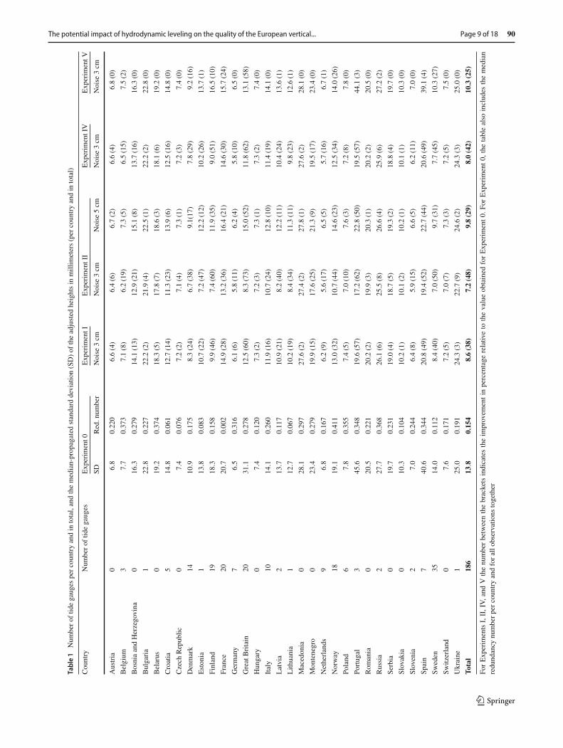
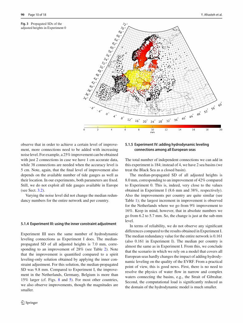
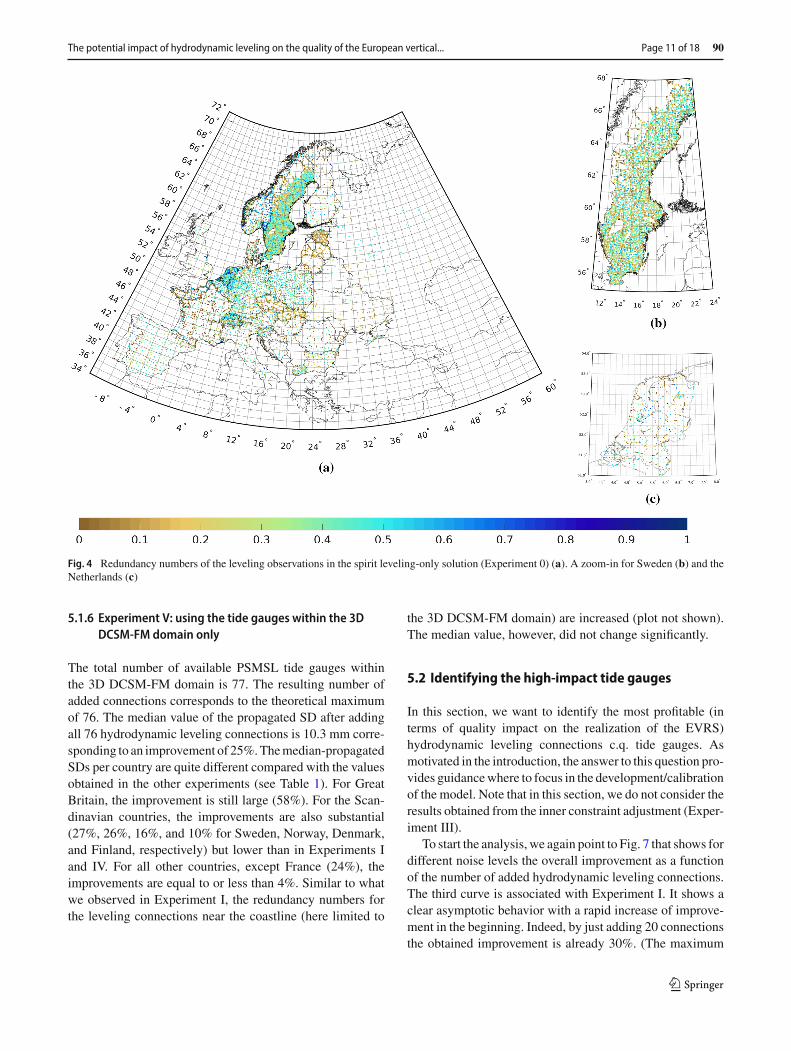
Figure 3 shows a map of the SDs of the adjusted heightsfor the spirit leveling-only solution (i.e., the solution whichserves as a reference in experiments I, II, IV, and V). Theycover a broad range of values, between ∼ 5 and ∼ 75 mm.The median value is 13.8 mm. Table 1 shows the medianSD per country. Both Table 1 and Fig. 3 clearly show thelarge regional deviations; the values are lowest at the cen-ter (including Belgium, Germany, the Netherlands, Austria,Czech Republic, and Poland) and increase toward the mar-gins. The mentioned countries all have high-quality levelingdata (see Table 3 of Sacher and Liebsch (2019)). Moreover,most of the datum points are located in these countries (seeFig. 1). As mentioned before, the propagated SDs are notonly affected by the precision of the observations, but alsoby the heightmarker distance to the datumpoints (Sacher andLiebsch 2019). The absence of a datumpoint in the Scandina-vian Peninsula explains why in Finland and Sweden (despitehaving high-quality leveling data) the adjusted height SDsare high compared to those in the center. Figure 4 shows amap of the redundancy numbers, and Table 1 presents themedian redundancy number per country and for the entirenetwork. Overall, the redundancy numbers are small withvalues ranging from 0.002 (France) to 0.411 (Norway). Thelow value for France can be explained by the fact that theFrench leveling network contains many height markers thatare only connected to one other height marker (see Fig. 1).The better the network is connected, the higher the redun-dancy numbers would be. By adding hydrodynamic levelingobservations, we expect to increase the redundancy numbersin the coastal areas.
5.1.2 Experiment I: allowing for connections within basinsonly
Given the total number of 186 candidate tide gauges(Sect. 3.2) spread over 4 separate sea basins, the numberof independent connections we can add is 182 (note that itis only allowed to establish connections within the same seabasins).
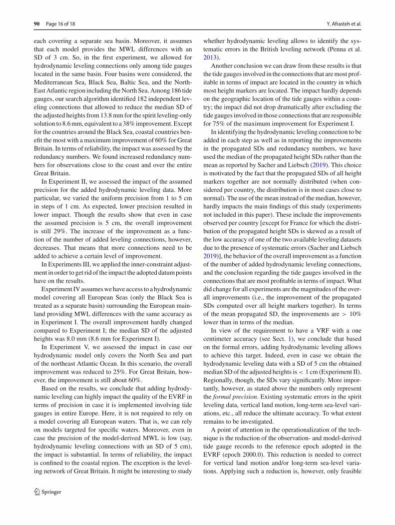
Adding all 182 connections reduces the median-propaga-ted SD of all adjusted heights from 13.8 to 8.6 mm. Thiscorresponds to an improvement of 38%. The improvementdiffers strongly per country as shown in Table 1; values rangefrom 1% (Slovakia) to 60% (Great Britain). We observelarger improvements for coastal countries, except for thecountries which are located along the Black Sea (see Fig. 5).We also notice a more significant improvement for coastalcountries at the perimeter of the UELN network (i.e., Portu-
gal, Spain, Great Britain, and the Scandinavian countries).The lower improvements for the Black Sea countries areexplained by the fact that hydrodynamic leveling connectionsthat link the Black Sea to the other European seas were notallowed. The reasonwhy the impact is largest inGreat Britaincan be understood when we consider that the existing con-nection of theGreat Britain leveling network to the remainingpart of the UELN is extremely weak; it is connected by justtwo leveling campaigns through the channel tunnel. Sincethere are many tide gauges in Great Britain, hydrodynamicleveling allows to tie Great Britain much stronger to the restof the UELN.
In terms of reliability, we observe increased redundancynumbers for the spirit leveling observations near the coastline(see Fig. 6). For most of these observations, the improvementis between 0.02 and 0.1. For about 1% of the observationsthe improvement is larger, the maximum being 0.9. In GreatBritain, the numbers increase almost throughout the wholecountry. Here, they range between 0 and 0.5. The medianredundancy number for Great Britain improves from 0.278 to0.462 (note that in computing this value the redundancy num-bers associated to the hydrodynamic leveling observationsare excluded). For the other countries, we hardly observedany change in the median redundancy number. (For that rea-son, they are not included in Table 1.) This is reflected bythe minor change in the median redundancy number for thewhole network (0.161 versus 0.154 for Experiment 0).
5.1.3 Experiment II: varying the noise level
The total number of added connections is the same as inExperiment I. Table 1 shows the median SDs when assum-ing a noise SD of 1 and 5 cm for each hydrodynamic levelingconnection. The values corresponding to the other noise lev-els are in between these values (the ones corresponding to anoise level of 3 cm are those of Experiment I). As expected,the quality impact lowers with increasing noise level. Forthe most optimistic scenario, we found an improvement of48%; however, for a noise level of 5 cm we still gain 29%.As expected, the values are quite different per country butshow the same behavior for different noise levels. We alwaysobserve the largest improvement in Great Britain and Por-tugal, though the magnitude decreases with increasing noiselevel (see Table 1).
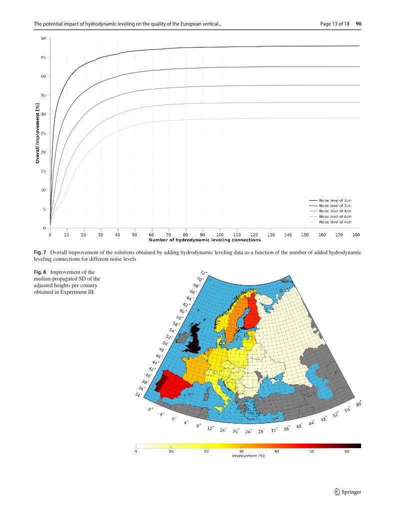
Figure 7 shows for all considered noise levels the improve-ment of the overall median-propagated height SD (i.e.,computed over all height markers) as a function of the num-ber of added hydrodynamic leveling connections. We noticethat the decrease of the level of improvement achieved byadding all connections is not linearly related to the increaseof the noise level. Indeed, the distance between the curvesfor the number of added connections being equal to 182 getssmaller and smaller when the noise level goes up. We also
123
The potential impact of hydrodynamic leveling on the quality of the European vertical... Page 9 of 18 90
Table1
Num
berof
tidegauges
percountryandin
total,andthemedian-propagated
standard
deviation(SD)of
theadjusted
heightsin
millim
eters(per
countryandin
total)
Cou
ntry
Num
berof
tidegaug
esExp
erim
ent0
Exp
erim
entI
Exp
erim
entII
Exp
erim
entIV
Exp
erim
entV
SDRed.n
umber
Noise
3cm
Noise
3cm
Noise
5cm
Noise
3cm
Noise
3cm
Austria
06.8
0.22
06.6(4)
6.4(6)
6.7(2)
6.6(4)
6.8(0)
Belgium
37.7
0.37
37.1(8)
6.2(19)
7.3(5)
6.5(15)
7.5(2)
BosniaandHerzegovina
016
.30.27
914
.1(13)
12.9(21)
15.1(8)
13.7(16)
16.3(0)
Bulgaria
122
.80.22
722
.2(2)
21.9(4)
22.5(1)
22.2(2)
22.8(0)
Belarus
019
.20.37
418
.3(5)
17.8(7)
18.6(3)
18.1(6)
19.2(0)
Croatia
514
.80.06
112
.7(14)
11.3(23)
13.9(6)
12.5(16)
14.8(0)
Czech
Republic
07.4
0.07
67.2(2)
7.1(4)
7.3(1)
7.2(3)
7.4(0)
Denmark
1410
.90.17
58.3(24)
6.7(38)
9.1(17
)7.8(29)
9.2(16)
Eston
ia1
13.8
0.08
310
.7(22)
7.2(47)
12.2(12)
10.2(26)
13.7(1)
Finland
1918
.30.15
89.9(46)
7.4(60)
11.9(35)
9.0(51)
16.5(10)
France
2020
.70.00
214
.9(28)
13.2(36)
16.4(21)
14.6(30)
15.7(24)
Germany
76.5
0.31
66.1(6)
5.8(11)
6.2(4)
5.8(10)
6.5(0)
GreatBritain
2031
.10.27
812
.5(60)
8.3(73)
15.0(52)
11.8(62)
13.1(58)
Hungary
07.4
0.12
07.3(2)
7.2(3)
7.3(1)
7.3(2)
7.4(0)
Italy
1014
.10.26
011
.9(16)
10.7(24)
12.8(10)
11.4(19)
14.1(0)
Latvia
213
.70.11
710
.9(21)
8.2(40)
12.2(11)
10.4(24)
13.6(1)
Lith
uania
112
.70.06
710
.2(19)
8.4(34)
11.3(11)
9.8(23)
12.6(1)
Macedon
ia0
28.1
0.29
727
.6(2)
27.4(2)
27.8(1)
27.6(2)
28.1(0)
Mon
tenegro
023
.40.27
919
.9(15)
17.6(25)
21.3(9)
19.5(17)
23.4(0)
Netherlands
96.8
0.16
76.2(9)
5.6(17)
6.5(5)
5.7(16)
6.7(1)
Norway
1819
.10.41
113
.0(32)
10.7(44)
14.6(23)
12.5(34)
14.0(26)
Poland
67.8
0.35
57.4(5)
7.0(10)
7.6(3)
7.2(8)
7.8(0)
Portugal
345
.60.34
819
.6(57)
17.2(62)
22.8(50)
19.5(57)
44.1(3)
Rom
ania
020
.50.22
120
.2(2)
19.9(3)
20.3(1)
20.2(2)
20.5(0)
Russia
227
.70.36
826
.1(6)
25.5(8)
26.6(4)
25.9(6)
27.2(2)
Serbia
019
.70.23
119
.0(4)
18.7(5)
19.3(2)
18.8(4)
19.7(0)
Slovakia
010
.30.10
410
.2(1)
10.1(2)
10.2(1)
10.1(1)
10.3(0)
Slovenia
27.0
0.24
46.4(8)
5.9(15)
6.6(5)
6.2(11)
7.0(0)
Spain
740
.60.34
420
.8(49)
19.4(52)
22.7(44)
20.6(49)
39.1(4)
Sweden
3514
.00.11
28.4(40)
7.0(50)
9.7(31)
7.7(45)
10.3(27)
Switzerland
07.6
0.17
17.2(5)
7.0(7)
7.3(3)
7.2(5)
7.5(0)
Ukraine
125
.00.19
124
.3(3)
22.7(9)
24.6(2)
24.3(3)
25.0(0)
Total
186
13.8
0.15
48.6(38)
7.2(48)
9.8(29)
8.0(42)
10.3(25)
ForExp
erim
entsI,II,IV,and
Vthenu
mberbetw
eenthebracketsindicatestheim
provem
entin
percentage
relativ
eto
thevalueob
tained
forExp
erim
ent0.
ForExp
erim
ent0,
thetablealso
includ
esthemedian
redu
ndancy
numberpercoun
tryandforallo
bservatio
nstogether
123
90 Page 10 of 18 Y. Afrasteh et al.
Fig. 3 Propagated SDs of theadjusted heights in Experiment 0
observe that in order to achieve a certain level of improve-ment, more connections need to be added with increasingnoise level. For example, a 25% improvement canbeobtainedwith just 2 connections in case we have 1 cm accurate data,while 38 connections are needed when the accuracy level is5 cm. Note, again, that the final level of improvement alsodepends on the available number of tide gauges as well astheir location. In our experiments, both parameters are fixed.Still, we do not exploit all tide gauges available in Europe(see Sect. 3.2).
Varying the noise level did not change the median redun-dancy numbers for the entire network and per country.
5.1.4 Experiment III: using the inner constraint adjustment
Experiment III uses the same number of hydrodynamicleveling connections as Experiment I does. The median-propagated SD of all adjusted heights is 7.0 mm, corre-sponding to an improvement of 28% (see Table 2). Notethat the improvement is quantified compared to a spiritleveling-only solution obtained by applying the inner con-straint adjustment. For this solution, the median-propagatedSD was 9.8 mm. Compared to Experiment I, the improve-ment in the Netherlands, Germany, Belgium is more than15% larger (cf. Figs. 8 and 5). For most other countries,we also observe improvements, though the magnitudes aresmaller.
5.1.5 Experiment IV: adding hydrodynamic levelingconnections among all European seas
The total number of independent connections we can add inthis experiment is 184; instead of 4, we have 2 sea basins (wetreat the Black Sea as a closed basin).
The median-propagated SD of all adjusted heights is8.0 mm, corresponding to an improvement of 42% comparedto Experiment 0. This is, indeed, very close to the valuesobtained in Experiment I (8.6 mm and 38%, respectively).Also the improvements per country are quite similar (seeTable 1); the largest increment in improvement is observedfor the Netherlands where we go from 9% improvement to16%. Keep in mind, however, that in absolute numbers wego from 6.2 to 5.7 mm. So, the change is just at the sub-mmlevel.
In terms of reliability, we do not observe any significantdifferences compared to the results obtained in Experiment I.The median redundancy value for the entire network is 0.161(also 0.161 in Experiment I). The median per country isalmost the same as in Experiment I. From this, we concludethat the scenario in which we rely on a model that covers allEuropean seas hardly changes the impact of adding hydrody-namic leveling on the quality of the EVRF. From a practicalpoint of view, this is good news. First, there is no need toresolve the physics of water flow in narrow and complexwaters connecting the basins, e.g., the Strait of Gibraltar.Second, the computational load is significantly reduced asthe domain of the hydrodynamic model is much smaller.
123
The potential impact of hydrodynamic leveling on the quality of the European vertical... Page 11 of 18 90
Fig. 4 Redundancy numbers of the leveling observations in the spirit leveling-only solution (Experiment 0) (a). A zoom-in for Sweden (b) and theNetherlands (c)
5.1.6 Experiment V: using the tide gauges within the 3DDCSM-FM domain only
The total number of available PSMSL tide gauges withinthe 3D DCSM-FM domain is 77. The resulting number ofadded connections corresponds to the theoretical maximumof 76. The median value of the propagated SD after addingall 76 hydrodynamic leveling connections is 10.3 mm corre-sponding to an improvement of 25%.Themedian-propagatedSDs per country are quite different compared with the valuesobtained in the other experiments (see Table 1). For GreatBritain, the improvement is still large (58%). For the Scan-dinavian countries, the improvements are also substantial(27%, 26%, 16%, and 10% for Sweden, Norway, Denmark,and Finland, respectively) but lower than in Experiments Iand IV. For all other countries, except France (24%), theimprovements are equal to or less than 4%. Similar to whatwe observed in Experiment I, the redundancy numbers forthe leveling connections near the coastline (here limited to
the 3D DCSM-FM domain) are increased (plot not shown).The median value, however, did not change significantly.
5.2 Identifying the high-impact tide gauges
In this section, we want to identify the most profitable (interms of quality impact on the realization of the EVRS)hydrodynamic leveling connections c.q. tide gauges. Asmotivated in the introduction, the answer to this question pro-vides guidancewhere to focus in the development/calibrationof the model. Note that in this section, we do not consider theresults obtained from the inner constraint adjustment (Exper-iment III).
To start the analysis, we again point to Fig. 7 that shows fordifferent noise levels the overall improvement as a functionof the number of added hydrodynamic leveling connections.The third curve is associated with Experiment I. It shows aclear asymptotic behavior with a rapid increase of improve-ment in the beginning. Indeed, by just adding 20 connectionsthe obtained improvement is already 30%. (The maximum
123

90 Page 12 of 18 Y. Afrasteh et al.
Fig. 5 Improvement of themedian-propagated SD of theadjusted heights per countryobtained in Experiment I
Fig. 6 Difference between theredundancy numbers obtained inExperiments I and 0
123
The potential impact of hydrodynamic leveling on the quality of the European vertical... Page 13 of 18 90
Fig. 7 Overall improvement of the solutions obtained by adding hydrodynamic leveling data as a function of the number of added hydrodynamicleveling connections for different noise levels
Fig. 8 Improvement of themedian-propagated SD of theadjusted heights per countryobtained in Experiment III
123

90 Page 14 of 18 Y. Afrasteh et al.
Table 2 Standard deviation (SD) of spirit leveling-only solution (inmillimeter)where the inner constraint is used for the network adjustmentand the standard deviation (SD) and percentage of improvement (valuesin bracket) per country for Experiment III
Country Referencespirit levelingsolution
Experiment III
Austria 8.9 7.4 (17)
Belgium 7.9 5.8 (27)
Bosnia and Herzegovina 18.5 15.1 (18)
Bulgaria 24.7 23.4 (5)
Belarus 19.1 18.0 (6)
Croatia 16.6 13.5 (19)
Czech Republic 9.0 7.6 (15)
Denmark 8.4 6.7 (20)
Estonia 13.1 9.5 (27)
Finland 15.0 8.4 (44)
France 19.7 13.9 (30)
Germany 6.9 5.2 (25)
Great Britain 30.8 11.4 (63)
Hungary 9.9 8.6 (14)
Italy 15.0 12.2 (19)
Latvia 13.1 9.8 (25)
Lithuania 12.3 9.4 (23)
Macedonia 29.4 28.5 (3)
Montenegro 25.6 20.9 (18)
Netherlands 7.0 4.8 (31)
Norway 15.7 11.7 (25)
Poland 9.0 7.3 (18)
Portugal 44.6 19.1 (57)
Romania 22.2 21.2 (5)
Russia 26.5 25.6 (3)
Serbia 21.3 19.6 (8)
Slovakia 12.1 11.0 (9)
Slovenia 9.4 7.5 (20)
Spain 39.6 20.6 (48)
Sweden 9.4 6.2 (34)
Switzerland 8.3 6.9 (17)
Ukraine 25.9 25.0 (4)
Total 9.8 7.0 (28)
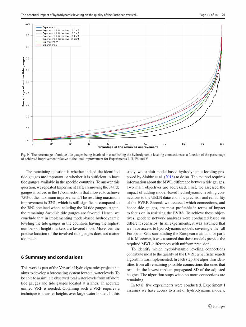
improvement in Experiment I is 38%.) Also, in the otherexperiments (plots not shown in the paper), we observe thisasymptotic behavior. To compare the results of the vari-ous experiments, we plotted in Fig. 9 the percentage ofunique tide gauges being involved in establishing the hydro-dynamic leveling connections as a function of the percentageof achieved improvement relative to the maximum improve-ment. From this plot, we observe that for all scenarios inwhichwe used the 3 cmnoise level (Experiments I, IV, andV)
75% of the maximum improvement can be achieved by usingonly 16–23% of the available tide gauges (which number is186, 186, and 77 for Experiments I, IV, and V, respectively).Only when we increase/decrease the noise level, more/lesstide gauges are needed to achieve a certain level of improve-ment (see the curves associated to Experiment II in Fig. 9).Still, even for a 5-cm noise level only 27% of the tide gaugesare needed to achieve 75% of the maximum improvement.This is a positive result as it shows that when adding a lim-ited number of hydrodynamic leveling connections betweena small number of tide gauges a substantial improvement inthe quality of the EVRF2019 can be achieved. Moreover, theanalysis suggests that adding more tide gauges than the onesconsidered in this study will not significantly increase theoverall level of improvement.
Next, we analyzed in more detail which tide gauges areinvolved in establishing the hydrodynamic leveling connec-tions that resulted in 75% of themaximum improvement. ForExperiments I, IV, and V, this involves 17, 15, and 9 connec-tions, respectively. In Experiment I and IV, tide gauges in 8and 7 countries are involved. Striking is that in both experi-ments, most connections involve tide gauges in Sweden (14in Experiment I and 13 in Experiment IV). Note that thesenumbers do not represent the number of unique tide gaugesinvolved. In some cases, tide gauges are involved in moreconnections. As seen earlier, increasing/decreasing the noiselevel (Experiment II) results in more/less connections beingneeded to achieve 75% of the maximum improvement. Thisbasically means more tide gauges per country; the numberof countries involved only slightly increased from 7 to 11when we increase the noise level from 1 to 5 cm. Again, byfar the Swedish tide gauges are favored most. They appearin 5, 9, 14, 17, and 17 connections by increasing the noiselevel from 1 to 5 cm. In Experiment V, the distribution overthe countries is different. Only tide gauges in 5 countries areinvolved, namely France, the Netherlands, Norway, Sweden,and Belgium. Here, tide gauges from Netherlands, Sweden,andNorway are favoredmost; they are used in 7, 5, and 4 con-nections, respectively. In both Belgium and France, only onetide gauge is used.
The reason why in Experiments I, II, and IV the Swedishtide gauges are favored can be understood as follows. Thecriterion used to identify the best set of hydrodynamic level-ing connections is based on themedian SD computed over allheight markers. In computing this median value, the countrywith the highest number of height markers will contributethe most. Sweden has the highest number of height mark-ers; 32% of all height markers are located in Sweden. For allother countries, the percentages are below 13%. Of course,other metrics to identify the best set of hydrodynamic lev-eling connections are possible resulting in other tide gaugesto be favored. For example, one might aim to minimize themedian SD for a specific country or some countries.
123
The potential impact of hydrodynamic leveling on the quality of the European vertical... Page 15 of 18 90
Fig. 9 The percentage of unique tide gauges being involved in establishing the hydrodynamic leveling connections as a function of the percentageof achieved improvement relative to the total improvement for Experiments I, II, IV, and V
The remaining question is whether indeed the identifiedtide gauges are important or whether it is sufficient to havetide gauges available in the specific countries. To answer thisquestion,we repeatedExperiment I after removing the 34 tidegauges involved in the 17 connections that allowed to achieve75% of the maximum improvement. The resulting maximumimprovement is 32%, which is still significant compared tothe 38% obtained when including the 34 tide gauges. Again,the remaining Swedish tide gauges are favored. Hence, weconclude that in implementing model-based hydrodynamicleveling the tide gauges in the countries having the highestnumbers of height markers are favored most. Moreover, theprecise location of the involved tide gauges does not mattertoo much.
6 Summary and conclusions
This work is part of the Versatile Hydrodynamics project thataims to develop a forecasting system for total water levels. Tobe able to assimilate observed totalwater levels fromoffshoretide gauges and tide gauges located at islands, an accurateunified VRF is needed. Obtaining such a VRF requires atechnique to transfer heights over large water bodies. In this
study, we exploit model-based hydrodynamic leveling pro-posed by Slobbe et al. (2018) to do so. The method requiresinformation about the MWL difference between tide gauges.Two main objectives are addressed. First, we assessed theimpact of adding model-based hydrodynamic leveling con-nections to the UELN dataset on the precision and reliabilityof the EVRF. Second, we assessed which connections, andhence tide gauges, are most profitable in terms of impactto focus on in realizing the EVRS. To achieve these objec-tives, geodetic network analyses were conducted based ondifferent scenarios. In all experiments, it was assumed thatwe have access to hydrodynamic models covering either allEuropean Seas surrounding the European mainland or partsof it. Moreover, it was assumed that these models provide therequired MWL differences with uniform precision.
To identify which hydrodynamic leveling connectionscontribute most to the quality of the EVRF, a heuristic searchalgorithmwas implemented. In each step, the algorithm iden-tifies from all remaining possible connections the ones thatresult in the lowest median-propagated SD of the adjustedheights. The algorithm stops when no more connections areremaining.
In total, five experiments were conducted. Experiment Iassumes we have access to a set of hydrodynamic models,
123
90 Page 16 of 18 Y. Afrasteh et al.
each covering a separate sea basin. Moreover, it assumesthat each model provides the MWL differences with anSD of 3 cm. So, in the first experiment, we allowed forhydrodynamic leveling connections only among tide gaugeslocated in the same basin. Four basins were considered, theMediterranean Sea, Black Sea, Baltic Sea, and the North-EastAtlantic region including theNorth Sea.Among 186 tidegauges, our search algorithm identified 182 independent lev-eling connections that allowed to reduce the median SD ofthe adjusted heights from13.8mm for the spirit leveling-onlysolution to 8.6mm, equivalent to a 38% improvement. Exceptfor the countries around the Black Sea, coastal countries ben-efit the most with a maximum improvement of 60% for GreatBritain. In terms of reliability, the impact was assessed by theredundancy numbers. We found increased redundancy num-bers for observations close to the coast and over the entireGreat Britain.
In Experiment II, we assessed the impact of the assumedprecision for the added hydrodynamic leveling data. Moreparticular, we varied the uniform precision from 1 to 5 cmin steps of 1 cm. As expected, lower precision resulted inlower impact. Though the results show that even in casethe assumed precision is 5 cm, the overall improvementis still 29%. The increase of the improvement as a func-tion of the number of added leveling connections, however,decreases. That means that more connections need to beadded to achieve a certain level of improvement.
In Experiments III, we applied the inner-constraint adjust-ment in order to get rid of the impact the adopted datumpointshave on the results.
Experiment IVassumeswehave access to a hydrodynamicmodel covering all European Seas (only the Black Sea istreated as a separate basin) surrounding the European main-land providing MWL differences with the same accuracy asin Experiment I. The overall improvement hardly changedcompared to Experiment I; the median SD of the adjustedheights was 8.0 mm (8.6 mm for Experiment I).
In Experiment V, we assessed the impact in case ourhydrodynamic model only covers the North Sea and partof the northeast Atlantic Ocean. In this scenario, the overallimprovement was reduced to 25%. For Great Britain, how-ever, the improvement is still about 60%.
Based on the results, we conclude that adding hydrody-namic leveling can highly impact the quality of the EVRF interms of precision in case it is implemented involving tidegauges in entire Europe. Here, it is not required to rely ona model covering all European waters. That is, we can relyon models targeted for specific waters. Moreover, even incase the precision of the model-derived MWL is low (say,hydrodynamic leveling connections with an SD of 5 cm),the impact is substantial. In terms of reliability, the impactis confined to the coastal region. The exception is the level-ing network of Great Britain. It might be interesting to study
whether hydrodynamic leveling allows to identify the sys-tematic errors in the British leveling network (Penna et al.2013).
Another conclusion we can draw from these results is thatthe tide gauges involved in the connections that aremost prof-itable in terms of impact are located in the country in whichmost height markers are located. The impact hardly dependson the geographic location of the tide gauges within a coun-try; the impact did not drop dramatically after excluding thetide gauges involved in those connections that are responsiblefor 75% of the maximum improvement for Experiment I.
In identifying the hydrodynamic leveling connection to beadded in each step as well as in reporting the improvementsin the propagated SDs and redundancy numbers, we haveused the median of the propagated height SDs rather than themean as reported by Sacher and Liebsch (2019). This choiceis motivated by the fact that the propagated SDs of all heightmarkers together are not normally distributed (when con-sidered per country, the distribution is in most cases close tonormal). The use of themean instead of themedian, however,hardly impacts the main findings of this study (experimentsnot included in this paper). These include the improvementsobserved per country [except for France for which the distri-bution of the propagated height SDs is skewed as a result ofthe low accuracy of one of the two available leveling datasetsdue to the presence of systematic errors (Sacher and Liebsch2019)], the behavior of the overall improvement as a functionof the number of added hydrodynamic leveling connections,and the conclusion regarding the tide gauges involved in theconnections that are most profitable in terms of impact.Whatdid change for all experiments are themagnitudes of the over-all improvements (i.e., the improvement of the propagatedSDs computed over all height markers together). In termsof the mean propagated SD, the improvements are > 10%lower than in terms of the median.
In view of the requirement to have a VRF with a onecentimeter accuracy (see Sect. 1), we conclude that basedon the formal errors, adding hydrodynamic leveling allowsto achieve this target. Indeed, even in case we obtain thehydrodynamic leveling data with a SD of 5 cm the obtainedmedian SD of the adjusted heights is< 1 cm (Experiment II).Regionally, though, the SDs vary significantly. More impor-tantly, however, as stated above the numbers only representthe formal precision. Existing systematic errors in the spiritleveling data, vertical land motion, long-term sea-level vari-ations, etc., all reduce the ultimate accuracy. To what extentremains to be investigated.
A point of attention in the operationalization of the tech-nique is the reduction of the observation- and model-derivedtide gauge records to the reference epoch adopted in theEVRF (epoch 2000.0). This reduction is needed to correctfor vertical land motion and/or long-term sea-level varia-tions. Applying such a reduction is, however, only feasible
123

The potential impact of hydrodynamic leveling on the quality of the European vertical... Page 17 of 18 90
if the tide gauge records are sufficiently long and all neededmetadata are available. An example of needed metadata isthe epoch when the tide gauge benchmark is connected tothe height system by means of leveling.
In a future work, we will derive a proper stochastic modelfor the hydrodynamic leveling dataset. Moreover, we willimplement the method using the 3D DCSM-FM model cur-rently under development. The upcoming release of themodel will expand the model domain to the Baltic Sea. Thiswould allow to establish hydrodynamic leveling connectionsamong the North Sea and Baltic Sea tide gauges. At the sametime, a more beneficial idea might be to launch a Europeanproject to develop regional hydrodynamic models to imple-ment hydrodynamic leveling at the European scale.
Acknowledgements This study was performed in the framework of theVersatile Hydrodynamics project, funded by the Netherlands Organiza-tion for Research (NWO). This support is gratefully acknowledged. Wethank the editor and three anonymous reviewers for their constructiveremarks and corrections, which helped us to improve the quality of themanuscript.
Declarations
Author contributions CS proposed the initial idea. YA, CS, MV, andRK designed the algorithm and experiments. YA and CS developed thesoftware and wrote the manuscript. All analyzed the results of the studyand reviewed the manuscript.
Data availability The UELN data are provided by the Federal Agencyfor Cartography and Geodesy (BKG). These data are not publicly avail-able. The tide gauge locations are obtained from the publicly availablePSMSL database (https://www.psmsl.org/data/obtaining/).
Open Access This article is licensed under a Creative CommonsAttribution 4.0 International License, which permits use, sharing, adap-tation, distribution and reproduction in any medium or format, aslong as you give appropriate credit to the original author(s) and thesource, provide a link to the Creative Commons licence, and indi-cate if changes were made. The images or other third party materialin this article are included in the article’s Creative Commons licence,unless indicated otherwise in a credit line to the material. If materialis not included in the article’s Creative Commons licence and yourintended use is not permitted by statutory regulation or exceeds thepermitted use, youwill need to obtain permission directly from the copy-right holder. To view a copy of this licence, visit http://creativecommons.org/licenses/by/4.0/.
References
AignerM, Ziegler GM (1998) Cayley’s formula for the number of trees.In: Proofs fromTHEBOOK. Springer, Berlin, pp 141–146. https://doi.org/10.1007/978-3-662-22343-7_22
Amiri-Simkooei AR, Asgari J, Zangeneh-Nejad F, Zaminpardaz S(2012) Basic concepts of optimization and design of geodeticnetworks. J Surv Eng 138(4):172–183. https://doi.org/10.1061/(asce)su.1943-5428.0000081
Amjadiparvar B, Rangelova E, SiderisMG (2015) The GBVP approachfor vertical datum unification: recent results in North America. JGeod 90(1):45–63. https://doi.org/10.1007/s00190-015-0855-8
AmosMJ, FeatherstoneWE (2008) Unification of New Zealand’s localvertical datums: iterative gravimetric quasigeoid computations. JGeod 83(1):57–68. https://doi.org/10.1007/s00190-008-0232-y
BaardaW (1968)A testing procedure for use in geodetic networks, NewSeries 2. Publication on Geodesy, Delft, p 2
Cartwright DE, Crease J (1963) A comparison of the geodetic referencelevels of England and France by means of the sea surface. P RoySoc Lond A Mat 273(1355):558–580
Catalão J, Sevilla M (2008) The use of ICAGM07 geoid model forvertical datum unification on Iberia and Macaronesian islands.American Geophysical Union, Fall Meeting 2008, abstract 2008Dec
Deltares (2021) Delft3D flexible Mesh suite. https://content.oss.deltares.nl/delft3d/manuals/D-Flow_FM_User_Manual.pdf
Denker H (2015) A new European Gravimetric (Quasi)GeoidEGG2015. 26th IUGGGeneral Assembly, June 22–July 2, Prague,Czech Republic
Donnelly C, Andersson JC, Arheimer B (2015) Using flow signaturesand catchment similarities to evaluate the E-HYPE multi-basinmodel across Europe. Hydrol Sci J 61(2):255–273. https://doi.org/10.1080/02626667.2015.1027710
EMODnet bathymetry consortium (2018) EMODnet digital bathymetry(DTM 2018)
Featherstone W, Filmer M (2012) The north-south tilt in the Aus-tralian height datum is explained by the ocean’s mean dynamictopography. J Geophys Res Oceans. https://doi.org/10.1029/2012JC007974
Federal Geodetic Control Committee, et al (1984) Standards and speci-fications for geodetic control networks. NOAA, National GeodeticInformation Branch, N/CG17X2, Sect 2:1
Filmer MS, FeatherstoneWE (2012) A re-evaluation of the offset in theAustralian height datum between Mainland Australia and Tasma-nia. Mar Geod 35(1):107–119. https://doi.org/10.1080/01490419.2011.634961
Filmer MS, Featherstone WE, Claessens SJ (2014) Variance compo-nent estimation uncertainty for unbalanced data: application to acontinent-wide vertical datum. J Geod 88(11):1081–1093. https://doi.org/10.1007/s00190-014-0744-6
Filmer MS, Hughes CW, Woodworth PL, Featherstone WE, Bing-ham RJ (2018) Comparison between geodetic and oceanographicapproaches to estimate mean dynamic topography for verticaldatum unification: evaluation at Australian tide gauges. J Geod92(12):1413–1437. https://doi.org/10.1007/s00190-018-1131-5
Gerlach C, Rummel R (2012) Global height system unification withGOCE: a simulation study on the indirect bias term in the GBVPapproach. J Geod 87(1):57–67. https://doi.org/10.1007/s00190-012-0579-y
Heck B, Rummel R (1990) Strategies for solving the vertical datumproblem using terrestrial and satellite geodetic data. In: Sea sur-face topography and the Geoid. Springer, New York, pp 116–128.https://doi.org/10.1007/978-1-4684-7098-7_14
Hersbach H, Bell B, Berrisford P, Hirahara S, Horányi A, Muñoz-Sabater J, Nicolas J, Peubey C, Radu R, Schepers D et al (2020)The ERA5 global reanalysis. Q J RMeteorol Soc 146(730):1999–2049. https://doi.org/10.1002/qj.3803
Holgate SJ, Matthews A, Woodworth PL, Rickards LJ, Tamisiea ME,Bradshaw E, Foden PR, Gordon KM, Jevrejeva S, Pugh J (2013)New data systems and products at the permanent service for meansea level. J Coast Res 29(3):493–504. https://doi.org/10.2112/JCOASTRES-D-12-00175.1
Ihde J, Augath W, Sacher M (2002) The Vertical Reference Systemfor Europe. In: International association of Geodesy symposia.
123
90 Page 18 of 18 Y. Afrasteh et al.
Springer, Berlin, pp 345–350. https://doi.org/10.1007/978-3-662-04683-8_64
Lea DJ, Mirouze I, Martin MJ, King RR, Hines A, Walters D, ThurlowM (2015) Assessing a new coupled data assimilation system basedon the met office coupled atmosphere-land-ocean-sea ice model.Mon Weather Rev 143(11):4678–4694. https://doi.org/10.1175/mwr-d-15-0174.1
Mehlstäubler TE, Grosche G, Lisdat C, Schmidt PO, Denker H (2018)Atomic clocks for geodesy. Rep Progress Phys 81(6):064 401.https://doi.org/10.1088/1361-6633/aab409
Moritz H (2000) Geodetic Reference System 1980. J Geod 74(1):128–162. https://doi.org/10.1007/s001900050278
Müller J, Dirkx D, Kopeikin SM, Lion G, Panet I, Petit G, VisserPNAM (2017) High performance clocks and gravity field determi-nation. Space Sci Rev 214(1):5. https://doi.org/10.1007/s11214-017-0431-z
Ogundare JO (2018) Understanding least squares estimation and geo-matics data analysis. Wiley, New York. https://doi.org/10.1002/9781119501459.ch14
Penna NT, Featherstone WE, Gazeaux J, Bingham RJ (2013) Theapparent British sea slope is caused by systematic errors in thelevelling-based vertical datum. Geophys J Int 194(2):772–786.https://doi.org/10.1093/gji/ggt161
Permanent Service for Mean Sea Level (PSMSL) (Retrieved 01 Jun2020) Tide Gauge Data. http://www.psmsl.org/data/obtaining/
Proudman J (1953) Dynamical oceanography. Methuen, New YorkRummel R, Teunissen P (1988) Height datum definition, height datum
connection and the role of the geodetic boundary value prob-lem. Bull Géodésique 62(4):477–498. https://doi.org/10.1007/bf02520239
Sacher M, Liebsch G (2019) EVRF2019 as new realization ofEVRS. https://evrs.bkg.bund.de/SharedDocs/Downloads/EVRS/EN/Publications/EVRF2019_FinalReport.pdf?__blob=publicationFile&v=2
Sánchez L, Sideris MG (2017) Vertical datum unification for the Inter-national Height Reference System (IHRS). Geophysical JournalInternational p ggx025, https://doi.org/10.1093/gji/ggx025
Schwarz KP, Sideris MG, Forsberg R (1987) Orthometric heights with-out leveling. J Surv Eng 113(1):28–40
Seemkooei AA (2001a) Comparison of reliability and geometricalstrength criteria in geodetic networks. J Geod 75(4):227–233.https://doi.org/10.1007/s001900100170
Seemkooei AA (2001b) Strategy for designing geodetic network withhigh reliability and geometrical strength. J Surv Eng 127(3):104–117. https://doi.org/10.1061/(asce)0733-9453(2001)127:3(104)
Slobbe DC, Klees R, Verlaan M, Zijl F, Alberts B, Farahani HH (2018)Height system connection between island and mainland using ahydrodynamic model: a case study connecting the Dutch Wad-den islands to the Amsterdam ordnance datum (NAP). J Geod92(12):1439–1456. https://doi.org/10.1007/s00190-018-1133-3
Stammer D, Ray RD, Andersen OB, Arbic BK, Bosch W, Carrère L,ChengY,ChinnDS,DushawBD,EgbertGDet al (2014)Accuracyassessment of global barotropic ocean tide models. Rev Geophys52(3):243–282. https://doi.org/10.1002/2014rg000450
Tarjan R (1972) Depth-first search and linear graph algorithms. SIAMJ Comput 1(2):146–160
Teunissen PJG (2006) Network quality control. VSSDWilkinson K, von Zabern M, Scherzer J (2014) Global Freshwa-
ter Fluxes into the World Oceans. http://doi.bafg.de/BfG/2014/GRDC_Report_44.pdf
Woodworth PL, Hughes CW, Bingham RJ, Gruber T (2013) Towardsworldwide height system unification using ocean information.J Geod Sci 2(4):302–318. https://doi.org/10.2478/v10156-012-0004-8
Zijl F, Veenstra J, Groenenboom J (2020) The 3D Dutch continentalshelf model-flexible mesh (3DDCSM-FM). https://www.deltares.nl/app/uploads/2020/12/Development-of-a-3D-model-for-the-NW-European-Shelf-3D-DCSM-FM.pdf
123