the political economy of development: ppha 42310 lecture 8... · 2019-05-31 · basic models of...

The Political Economy of Development: PPHA 42310Lecture 8

James A. Robinson

Chicago

May 2, 2019

James A. Robinson (Chicago) PED May 2, 2019 1 / 21

Roots of Di¤erent Equilibria

We�ve now seen a few examples of di¤erent political equilibria.

In some parts of the world we have high levels of public goodprovision and incomes and political institutions that support this(maybe by creating accountability, of political competition, or abalance of power).

Maybe we also have social structures that support this (individualizedsocieties that stop kinship networks capturing politics or don�t lead tomass violence).

But these institutions are certainly endogenous and we�ve seen somebasic models of endogenous state capacity, democracy ...


Roots of Di¤erent Equilibria

What can we say about where these equilibria come from? How comesome parts of the world were able to establish equilibria thatgenerates much more socially desirable outcomes?

It�s obvious that we have a far from complete understanding of thisissue, and it�s obviously a historical one.

Many forces shaped the historical evolution of societies but let mefocus on two on which there is some empirical evidence

European colonialismlabor coercion


Economic institutions and economic performance

.

Log

GDP

per c

apita

, PPP

, in 1

995

Avg. Protection Against Risk of Expropriation, 1985-954 6 8 10

6

8

10

AGO

ARE

ARG

AUS AUTBEL

BFA BGD

BGR

BHR

BHS

BOL

BRABWA

CANCHE

CHL

CHN

CIVCMRCOG

COLCRI

CZE

DNK

DOM DZAECU

EGY

ESP

ETH

FINFRA

GAB

GBR

GHAGIN

GMB

GRC

GTM

GUY

HKG

HND

HTI

HUN

IDN

IND

IRL

IRN

ISLISR

ITA

JAMJOR

JPN

KEN

KOR

KWT

LKA

LUX

MAR

MDG

MEX

MLI

MLT

MNG

MOZ MWI

MYS

NER NGA

NIC

NLDNOR

NZL

OMN

PAK

PAN

PER

PHL

POL

PRT

PRY

QAT

ROM RUS

SAU

SDNSEN

SGP

SLE

SLVSUR

SWE

SYR

TGO

THATTO

TUNTUR

TZA

UGA

URY

USA

VEN

VNM

YEM

ZAF

ZAR ZMB

ZWE

Colonial Origins: Theory

Theory: those with political power more likely to opt for goodinstitutions when they will bene�t from property rights andinvestment opportunities.

Better institutions more likely when there are constraints on elites.

The colonial context: Europeans more likely to bene�t from goodinstitutions when they are a signi�cant fraction of the population, i.e.,when they settle

Lower strata of Europeans place constraints on elites when there aresigni�cant settlements.

Thus: European settlements ) better institutions

But Europeans settlements are endogenous. They may be more likelyto settle if a society has greater resources or more potential forgrowth.

Or less settlements when greater resources; East India Company andSpanish crown limited settlements.


Exogenous Source of Variation

Look for exogenous variation in European settlements: the diseaseenvironment

In some colonies, Europeans faced very high death rates because ofdiseases for which they had no immunity, in particular malaria andyellow fever.

Potential mortality of European settlers ) settlements ) institutions

Moreover, for many reasons, already discussed above, institutionspersist; so

Potential mortality of European settlers ) settlements ) past institutions) current institutions


Empirics: Colonial Origins of Comparative Development#1

Empirical setup: Two Stage Least-Squares (2SLS)Second stage: log income per capita = f(current economicinstitutions)First stage: current economic institutions = g(settler mortality)Data on potential European settler mortality. Work by the historianPhilip Curtin provides us with mortality rates of soldiers stationed inthe colonies in the early 19th century. Supplemented by data onmortality of Catholic bishops in Latin AmericaCurrent economic institutions proxied by protection againstexpropriation riskUseful to bear in mind that history generates variation in a cluster ofbroad institutions;Protection against expropriation risk proxying for many other sourcesof institutional variation


Settler mortality and current institutions

.

Avg

. Pro

tect

. Aga

inst

Ris

k E

xpro

pria

tion

Log Settler Mortality2 4 6 8

4

6

8

10

AGO

ARG

AUS

BFA

BGD

BHS

BOL

BRA

CAN

CHL

CIV

CMR

COG

COLCRI

DOM

DZAECUEGY

GAB

GHAGIN

GMB

GTM

GUY

HKG

HND

HTI

IDN

IND

JAM

KENLKA

MAR

MDG

MEX

MLI

MYS

NER

NGANIC

NZL

PAKPAN

PER

PRY

SDN

SEN

SGP

SLE

SLV

SUR

TGO

TTO

TUNTZA

UGA

URY

USA

VEN

VNM

ZAF

ZAR

The first stage

First Stage Regressions:Dependent variable is protection against risk of expropriation

All former colonies

All former colonies

All former colonies

Without neo-Europes

Settler Mortality -0.61 -0.5 -0.43 -0.37(0.13) (0.15) (0.19) (0.14)

Latitude 2.34(1.37)

Continent Dummies (p-value) [0.25]

R-Squared 0.26 0.29 0.31 0.11Number of Observations 63 63 63 59

Standard errors in parenthesesSample limited to countries for which have GDP per capita data

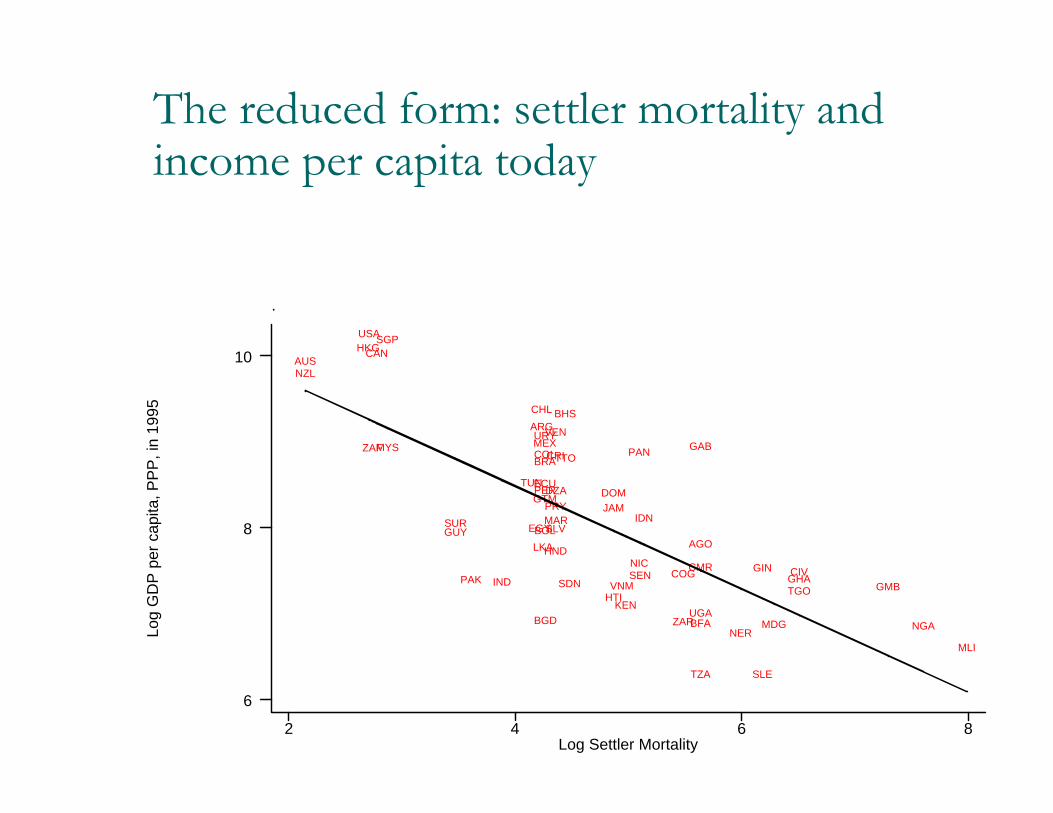
The reduced form: settler mortality and income per capita today

.

Log

GD

P p

er c

apita

, PP

P, i

n 19

95

Log Settler Mortality2 4 6 8

6

8

10

AGO

ARG

AUS

BFABGD

BHS

BOL

BRA

CAN

CHL

CIVCMRCOG

COLCRI

DOMDZAECU

EGY

GAB

GHAGIN

GMB

GTM

GUY

HKG

HND

HTI

IDN

IND

JAM

KEN

LKA

MAR

MDG

MEX

MLI

MYS

NERNGA

NIC

NZL

PAK

PAN

PERPRY

SDNSEN

SGP

SLE

SLVSUR

TGO

TTO

TUN

TZA

UGA

URY

USA

VEN

VNM

ZAF

ZAR

The causal effect of institutions: basic 2SLS estimates

Second Stage Regressions:Dependent variable is log GDP per capita in 1995

All former colonies

All former colonies

All former colonies

Without neo-Europes

Protection Against Risk of 0.99 1.11 1.19 1.43Expropriation, 1985-95 (0.17) (0.26) (0.39) (0.45)Latitude -1.61

(1.57)Continent Dummies (p-value) [0.09]

Number of Observations 63 63 63 59

The causal effect of institutions: robustnessSecond Stage Regressions: all former colonies Dependent variable is log GDP per capita in 1995Instrument is:

Log Settler Mortality



Log Settler Mortality Yellow Fever

Protection Against Risk of 1.07 0.98 0.87 1.18 0.82Expropriation, 1985-95 (0.27) (0.17) (0.32) (0.84) (0.22)Temperature (p-value) [0.71]

Humidity (p-value) [0.64]

Malaria -0.28(0.59)

Life Expectancy -0.014(0.07)

Number of Observations 63 63 62 62 63


Is the empirical approach valid?

Clearly no reverse causality, mortality rates refer to two centuries ago

Is the exclusion restriction of the 2SLS valid?

Plausible: yellow fever, malaria and gastrointestinal diseases a¤ectingEuropeans had much less e¤ect on native inhabitants, who hadacquired and genetic immunity.

Mortality rates of local troops very similar in di¤erent regions despitevery large di¤erences in European mortality rates.



Is the empirical approach valid? (continued)

Check validity further by controlling for potential sources of directe¤ect, including latitude, measures of geography, current prevalenceof malaria and life expectancy.

Use only variation due to yellow fever, which is now mostlyeradicated, thus less likely to have direct e¤ect.

Use over identi�cation tests to check validity of instrument.

Also note that if the instrument is valid, it solves theerrors-in-variables problem.

These checks all support the validity of the approach.

Note: not estimating the causal e¤ect of being colonized vs. notcolonized


Main Results

Very large causal e¤ects of institutions on long-run growth.

Di¤erences in institutions account for over 34 of the variation inincome per capita today (long-run e¤ect)

Robust in di¤erent subsamples

Robust to controlling for continent dummies

Robust to controlling for latitude, whether landlocked, temperature,humidity

Robust to controlling for current prevalence of malaria and lifeexpectancy

Robust when exploiting only yellow fever

Overidenti�cation tests supportive.

Also no evidence of any e¤ect of geography or religion on long rungrowth


The Role of Geography

No causal e¤ect of geography.

How do we think of the correlation between geography (e.g., latitude)and income?

This is caused by omitted factors;

Geography correlated with institutions because of the naturalexperiment of European colonialism.

Tropical areas ended up with worse institutions, because they tendedto be richer and more densely-populated circa 1500. They attractedfewer European settlers.

Also no universal causal e¤ect of geography on institutions.

Relationship created in a particular historical juncture.


Long Run E¤ects of Coercion

A systematic fact is that coercion of workers and people is involved inthe creation of extractive institutions. In all parts of the world thetransition towards inclusive institutions has coincided with reductionsin coercion.

This is true in Europe with the collapse of serfdom in the lateMedieval period. It is clear that the parts of Europe (East of theDanube) where serfdom lasted longer are much less developedeconomically and did not bene�t until the 20th century (after theabolition of serfdom) from the Industrial Revolution.

Understanding the role of coercion, rather than simply the impact ofextractive institutions, is di¢ cult but today I want to show you that ithas left a long and negative shadow in terms of its impact ofeconomic development.


Slavery and the Slave Trade

Perhaps the most studied example of the impact of labor coercion isthe African slave trade.

There is a large academic literature (see Chapter 12 of WNF) on howthe slave economy and its legacy kept the US South relatively pooruntil the 1950s and 1960s.

Slavery had ancient roots in Africa but it is also clear that theemergence of large external markets for slaves led to theintensi�cation of slavery within Africa (WNF Chapter 9)

Most slaves seem to have been captured in wars and states grewbased on slaving (Oyo, Dahomey and Asante in West Africa).

The warfare and general reduction in population have beenhypothesized to have reduced the size and centralization of Africanstates and even to have made African populations more ethnicallyfragmented.


Some Estimates of the Economic Impact in Africa

Nathan Nunn has constructed some estimates of the negative e¤ectsof the slave trade on income per-capita in Africa.

To do this he used a very wide variety of sources, mostly shippingrecords, plantation records and sales receipts, from which he took theethnicity/origin of the slaves. he used this data to construct estimatesof where slaves came from in Africa and he matched this to themodern nation states.

He found that the intensity of slaving is negatively correlated withincome per-capita today and also institutional quality.

The quantitative e¤ects are large and signi�cant. For example, a fallof one standard deviation in the extent of slaving raises incomeper-capita from the mean of $1,249 to $1,864 a 50% increase.

Nevertheless, to go from the maximal amount of slaving (Angola) tozero would only raise income per-capita by 150%, far less than theincome gap between Africa and rich countries today.


Magnitude of the Slave Trades

Slave Trade 1400–1599 1600–1699 1700–1799 1800–1913 1400–1913

trans-Atlantic 188,108 597,444 8,253,885 3,709,081 12,748,518

trans-Saharan 700,000 435,000 865,000 1,066,143 3,066,143

Red Sea 400,000 200,000 200,000 505,400 1,305,400

Indian Ocean 200,000 100,000 428,000 395,300 1,123,300

Total 1,488,108 1,332,444 9,746,885 5,675,924 18,243,361

Total/year 7,441 13,324 97,469 50,230 35,562

Data Sources

1. Shipping Data

• Know the total number of slaves exported from each

port or region of Africa.

2. Ethnicity Data

• Observe the ethnic origins of a subsample of slaves

shipped outside of Africa.

Shipping Data

• Atlantic slave trade.

– Know port of embarkation.

• Indian Ocean slave trade.

– Know region of embarkation.

• Saharan slave trade.

– Know slaves’ destinations.

– Know which caravan slaves arrived on.

• Red Sea slave trade.

– Know port of embarkation.

Ethnicity Data

• Atlantic slave trade.

– 46 samples, 88,616 slaves, 480 ethnicities

• Indian Ocean slave trade.


• Saharan slave trade.


• Red Sea slave trade.

– 1 sample, 5 slaves, 2 ethnicities

Table 2: Slave Ethnicity Data: Trans-Atlantic Slave Trade

Num. Num.

Region Years Ethnic. Obs. Record Type

Valencia, Spain 1482–1516 25 2,651 Crown Records

Dominican Republic 1547–1591 11 27 Records of Sale

Peru 1548–1560 16 207 Records of Sale

Mexico 1549 12 83 Plantation Accounts

Peru 1560–1650 27 7,573 Notarial Records

Lima, Peru 1583–1589 15 288 Baptism Records

Colombia 1589–1607 6 20 Various Records

Mexico 1600–1699 26 406 Records of Sale

Dominican Republic 1610–1696 20 55 Government Records

Chile 1615 6 140 Sales Records

Lima, Peru 1630–1702 33 411 Parish Records

Peru (Rural) 1632 25 307 Parish Records

Lima, Peru 1640–1680 33 936 Marriage Records

Colombia 1635–1695 6 19 Slave Inventories

Guyane (French Guiana) 1690 12 69 Plantation Records

Colombia 1716–1725 19 58 Government Records

French Louisiana 1717–1769 109 6,315 Notarial Records

Dominican Republic 1717–1827 8 15 Government Records

South Carolina 1732–1775 39 907 Runaway Notices

Colombia 1738–1778 11 109 Various Records

Spanish Louisiana 1770–1803 109 6,615 Notarial Records

St. Dominique (Haiti) 1771–1791 30 5,433 Sugar Plantations

St. Dominique (Haiti) 1778–1791 36 1,293 Coffee Plantations

Guadeloupe 1788 8 55 News Paper Report

Cuba 1791–1840 55 3,218 Slave Registers

St. Dominique (Haiti) 1796–1797 51 5,723 Plantation Inventories

Table 2: Slave Ethnicity Data: Trans-Atlantic Slave Trade, continued

Num. Num.

Region Years Ethnic. Obs. Record Type

American Louisiana 1804–1820 109 5,389 Notarial Records

From Central Sudan 1804–1850 58 108 Slave Interviews

Salvador, Brazil 1808–1842 19 662 Records of Manumission

Trinidad 1813 115 13,346 Slave Registers

St. Lucia 1815 44 2,638 Slave Registers

St. Kitts 1817 36 2,886 Slave Registers

Berbice (Guyana) 1819 40 1,142 Slave Registers

Salvador, Brazil 1819–1836 14 1,105 Manumission Certificates

Salvador, Brazil 1820–1835 13 1,341 Probate Records

Sierra Leone 1821–1824 68 638 Child Registers

Rio de Janeiro, Brazil 1826–1837 36 1,906 Prison Records

Anguilla 1827 8 30 Slave Registers

Rio de Janeiro, Brazil 1830–1852 470 4,034 Free Africans’ Records

Rio de Janeiro, Brazil 1833–1849 39 1,735 Death Certificates

Salvador, Brazil 1835 13 277 Court Records

Salvador, Brazil 1838–1848 11 250 Slave Registers

Sierra Leone 1848 63 7,302 Linguistic and British Census

Salvador, Brazil 1851–1884 13 410 Records of Manumission

Salvador, Brazil 1852–1888 10 294 Slave Registers

Kikoneh Island, Sierra Leone 1896–1897 11 190 Fugitive Slave Records

Total 88,616

Table 3: Slave Exports, 1400–1913: Top 10 countries

Atlantic Indian Ocean Saharan Red Sea Total Percent

Country Exports Exports Exports Exports Exports of Total

Nigeria 1,997,342 0 329,185 0 2,326,526 13%

Zaire 2,184,318 0 0 0 2,184,318 12%

Angola 2,095,149 0 0 0 2,095,149 12%

Ghana 1,459,691 0 0 0 1,459,691 8%

Ethiopia 0 0 449,023 768,701 1,217,724 7%

Sudan 0 0 910,593 263,456 1,174,049 7%

Benin 916,913 0 12,050 0 928,963 5%

Mozambique 327,773 382,884 0 0 710,657 4%

Congo 706,931 0 0 0 706,931 4%

Angola

Burundi

BeninBF

Botswana

Central Afr Rep

Ivory CoastCameroon Congo

Comoros

Cape Verde

Djibouti

Algeria

Egypt

Ethiopia

Gabon

Ghana

Guinea

Gambia

Guinea Bissau

Equitorial Guinea

Kenya LiberiaLesotho

Morocco

Madagascar Mali

Moz

Mauritania

Mauritius

Malawi

Namibia

Niger

Nigeria

Rwanda

SudanSenegal

SL

Somolia

Swaziland

Seychelles

Chad Togo

Tunisia

Tanzania

Uganda

S Africa

Zaire

Zambia

Zimbabwe

57

.51

0L

og

19

98

Rea

l p

er C

apit

a G

DP

−4 0 5 11Log Total Slave Exports per 1,000 km sq of Land Area

Data source: PWT and author’s calculations

(beta coef = −.60, t−stat = 5.37)

Relationship Between Current Income and Past Slave Exports

Tunisia

Botswana

Lesotho

Cape Verde

Swaziland

S Africa

Algeria

Central Afr Rep

Mauritania

Sychelles

Mauritius

Zimbabwe

EthiopiaKenya

Chad

Burundi

Rwanda

Zambia Niger

Uganda

Gabon

Equitorial Guinea NamibiaIvory Coast

Madgas

Morocco

Cameroon

Mali

Liberia

Moz

Burkina Faso

Zaire

Angola

Egypt

SudanCongo

Djibouti

Somolia

Guinea

Tanzania

Senegal

TogoGuinea Bissau

Nigeria

Malawi

Benin

Sierra LComoros

Ghana

Gambia

−1

.60

2.3

E(L

og

19

98

Rea

l p

er C

apit

a G

DP

| X

)

−13 0 9E(Log Total Slave Exports | X)

(coef = −.11, t−stat = −5.11)

Partial Correlation Plot: Log Income and Slave Exports

AGO

BDI

BEN

BFA

BWA

CAF CIV

CMR COG

COM

CPV

DJI

DZA

EGY

ETH

GAB

GHA

GIN

GMBGNB

GNQ

KEN

LBR

LBY

LSO

MAR

MDG

MLIMOZ

MRT

MUS

MWI

NAMNER

NGA

RWA

SDNSEN

SLESOM

SWZ

SYC

TCD

TGO

TUN

TZA

UGA

ZAF

ZAR

ZMB

ZWE

0.5

1.1

Eth

nic

Fra

ctio

nal

izat

ion


(beta coef = .60, t−stat = 5.21)

Current Ethnic Fractionalization and Past Slave Exports

AGO

BDI

BEN

BFA

BWA

CAF

CIV

CMR

COG

COM

CPV

DJI

ETH

GAB

GHA

GINGMB

GNBGNQ

KEN

LBR

LSO

MDG

MLI

MOZMRT

MUS

MWI

NAM

NER

NGA

RWA

SDN

SEN

SLESOM

STP

SWZSYC

TCD

TGO

TZAUGA

ZAR

ZMB

ZWE

0.5

1.1

19

th C

entu

ry S

tate

Cen

tral

izat

ion


(beta coef = −.46, t−stat = 3.43)

19th Century State Centralization and Past Slave Exports

AGO

BDI

BEN

BFA

BWA

CAF

CIVCMR COG

DZA

EGY

ETH

GABGHA

GIN

GNB

GNQ

KEN

LBR

LSO

MAR

MDGMLI

MOZ

MRT

MWI

NAM

NER

NGA

RWA

SDNSEN

SLE

SOM

SWZ

TCD

TGO

TUN

TZAUGA

ZAF

ZMB

ZWE

01

23

45

Pre

val

ence

of

Do

mes

tic

Sla

ver

y i

n 1

9th

Cen

tury


Data source: Ethnographic Atlast and author’s calculations

(beta coef = .58 , t−stat = 4.61)

Log Slave Exports and Domestic Slavery in the 19th Century

Why did Africa specialize in Exporting Slaves?

One line of argument (the �Domar Hypothesis�) emphasizes thatslavery became endemic in Africa because population density was low.This meant that if there had been a labor market wages (marginalproduct of labor) would have been very high, hence there was a bigincentive to enslave in order to avoid paying high wages.

This argument suggests that slaves would have been very productiveif used in Africa.

So why were slaves sold and shipped to the Americas?

This becomes even more puzzling when we observe the hugeine¢ ciencies (if that doesn�t sound too inhumane) in this process.Around 10-20% of captives died en route between Africa and theAmericas. Far more died in the violence of capture or on the way tobe sold (Joseph Miller estimated that 50% of the slaves caught in theinterior of Angola died before being sold at the coast).


So why the Export?

The most compelling (to me) approach is that though it could bethat the physical marginal product of labor was high in Africa, thee¢ ciency of the economy was actually low because economicinstitutions did not encourage production.

One reason is that in places which lacked centralized states there wasfeuding/raiding/insecurity of property rights, recall the Nuer in theSudan. This made the return to production and to labor low, even ifthe physical product was high.

Another example would be the form of property rights to land whichdid not promote security of tenure and undermined investmentincentives.

Thus when opportunities to sell labor to Europeans came, theopportunity cost of doing so was low.


The Role of Slavery and the Slave Trade

Very plausible that the slave trade had signi�cant negative e¤ectsalong the lines postulated by many historians and quanti�ed by Nunn.

But the e¤ect on income is much less than the income di¤erencesbetween Africa and the rest of the world.

Also, as Jan Vansina pointed out in Central Africa, one sees verysimilar institutional dynamics in places which were and which werenot impacted by the slave trade.

The slave trade and domestic slavery are part of the story of whyAfrica is poor, but they are part of a path dependent process. Africaselected into the slave trade because its institutions were already bad.


Slavery and Trust

Nathan Nunn extended his work with a fascinating study on theimpact of the slave trade on inter-personal trust in modern Africa.

He extended his slave database to the ethnicity level (rather than justworking with the country as the unit of analysis).

He matched the slave trade data with contemporary data from theAfrobarometer on the extent to which people trust each other.


The Andean Mining Mitas

This was one of the most important systems of forced labor in LatinAmerica.

In 1545 silver was discovered in El Cerro Rico (the rich hill) in Potosí.In the 1570s Viceroy Francisco de Toledo reorganized the colony ofPeru with an eye to increasing the revenues of the colonial state. Heorganized in Potosí mita, which was to last until the 1820s. Othermitas operated, such as to the mercury mines in Huancavelica.

The mita (mit�a in Quechua means �a turn�) built on earlier Indiantribute systems for generating labor and basically stipulated that1/7th of the adult males from a catchment area had to be in themines of Potosí.


Figure 1

!

!

Study Boundary

Mita Boundary

5000 m

0 m

Potosi

Huancavelica

UyuniSalt Flat

The mita boundary is in black and the study boundary in light gray. Districts falling insidethe contiguous area formed by the mita boundary contributed to the mita. Elevation is shownin the background.

47

Figure 2

!

!

!! !!!

! !!

!

!

!

! !

!

!

!

!

!

!

!

!

!

!

!

!

!

!

!

!

!

!

!

!

!

!

!

!

!

!

!

!

!

!

!!

!

!

!

!

!

!

!

!

!

!

!

!

!

!

!

!

!

!

!

!

!

!

!

!

!

!

!

!

!

!

!

!

!

!!

!

!

!

!

!!

!

!

!

!

!

!

!

!

!

!

!

!!

!

!

!!

!

!

!

!

!

!

!

!

!

!

!

!

!

!

!

!

!

!

!

!

!

!

!

!

!

!

! !

!

!

!

!

!

!

!

!

!

!

!

!

!

!

!

!

!

!

!

!

!

!

!

!!

!

!

!

!

!

!

!

!

!

!

!

!

!

!!

!

!!

!

!

!

!

!

!

!

!

!!

!

!

!

!

!

!

!

!

!!

!

!

!

!

!

! District Capitals

Study Boundary

District Boundaries

Grid Cells

>5000 m

0 m

Mita districts fall between the two thick lines. The circles show district capitals within 50kilometers of the mita boundary. The boundaries for the 20 x 20 km grid cells - used in Table1 - are in light gray. District boundaries are in black, and elevation is shown in thebackground.

48

Did the Mita have a Persistent E¤ect?

This has been investigated by Melissa Dell (�The Persistent E¤ects ofPeru�s Mining Mita�) using a very nice research design exploiting theregression discontinuity methodology.

She took micro World Bank Living Standards data from Peru andmatched it to the boundary of the mita.

One problem is that at some of the points on the boundary, altitudeand ethnicity of dominant Indian group jumps all at the same time.Hence it is di¢ cult to identify the e¤ect of the mita as opposed toethnicity or altitude. However, this is not for part of the border inPeru.

She �nds that average household consumption is about 1/3 lower inmita areas close to the boundary compared to non-mita areas.

This is robust to controlling for all sorts of household characteristics.


Mechanisms of Persistence

Just as important as this �nding is her evidence on mechanisms.

She shows that today, a proximate explanation for why mita areas arepoorer is that people there tend to be subsistence farmers and marketa smaller proportion of their crop.

One of the reasons for this seems to me infrastructure, density ofroads is much less in mita areas.

She also shows that historically haciendas formed outside the mitaareas because the Spanish colonial state wanted to protect the laborfore for the mines from exploitation by creoles. The elites whocontrolled the haciendas seem to have been much better at gettingpublic goods than people in the mita areas.


The Long Shadow of Extractive Institutions

One of the themes of WNF is that extractive institutions leave longpath dependent shadows.

I think that�s pretty obvious in the case of the US.

Still it doesn�t mean that policy is irrelevant or you can�t changethings. Things did change for the better in the US South in the 1950sand 1960s.

In Nunn�s individual level data, though it is true that if you are amember of an ethnic group that was subject to more intensive slaveryhistorically you tend to trust less today, it is also true that holdingthat constant, the more educated you are the more you trust people.Thus greater investment in education can overcome the legacy of theslave trade.


the political economy of development: ppha 42310 lecture 8... · 2019-05-31 · basic models of...

Documents