the nexus between agricultural productivity, oil prices
TRANSCRIPT

NEAR EAST UNIVERSITY
GRADUATE SCHOOL OF SOCIAL SCIENCES
BANKING AND FINANCE PROGRAM
THE NEXUS BETWEEN AGRICULTURAL
PRODUCTIVITY, OIL PRICES, ECONOMIC GROWTH,
AND FINANCIAL DEVELOPMENT IN THE USA
SIMBARASHE RABSON ANDREA
MASTER’S THESIS
NICOSIA
2018
NEAR EAST UNIVERSITY
GRADUATE SCHOOL OF SOCIAL SCIENCES
BANKING AND FINANCE PROGRAM
THE NEXUS BETWEEN AGRICULTURAL
PRODUCTIVITY, OIL PRICES, ECONOMIC GROWTH
AND FINANCIAL DEVELOPMENT IN THE USA
SIMBARASHE RABSON ANDREA
MASTER’S THESIS
THESIS SUPERVISOR
ASSOC. PROF. DR. TURGUT TÜRSOY
NICOSIA
2018
iii
ACCEPTANCE
We as the jury members certify "The Nexus Between Agricultural Productivity,
Oil Prices, Economic growth and Financial development in USA” prepared by
Simbarashe Rabson Andrea defended on 19 December 2018 has been found
satisfactory for the award of degree of Master.
JURY MEMBERS
……………………………….
Assoc. Prof. Dr. TURGUT TÜRSOY (Supervisor)
Near East University
Faculty of Economics and Administrative / Department of Banking and Finance
……………………………….
Assist. Prof. Dr. Nil GÜNSEL REŞATOĞLU
Near East University
Faculty of Economics and Administrative / Department of Banking and Finance
……………………………….
Assist. Prof. Dr. Behiye TÜZEL ÇAVUŞOĞLU
Near East University
Faculty of Economics and Administrative / Department of Economics
……………………………….
Prof. Dr. Mustafa Sağsan
Graduate School of Social Sciences
Director


i
DECLARATION
I Simbarashe Rabson Andrea, hereby declare that this dissertation entitled "The Nexus
Between Agricultural Productivity, Oil Prices, Financial Development And Economic
Growth In USA" has been prepared myself under the guidance and supervision of
“Assoc. Prof. Dr. Turgut Türsoy.” in partial fulfilment of The Near East University,
Graduate School of Social Sciences regulations and does not to the best of my knowledge
breach any Law of Copyrights and has been tested for plagiarism and a copy of the result
can be found in the Thesis.
The full extent of my Thesis can be accessible from anywhere.
My Thesis can only be accessed from the Near East University.
My Thesis cannot be accessible for (2) two years. If I do not apply for an extension
at the end of this period, the full extent of my Thesis will be accessible from
anywhere.
Date: 19th of December 2018
Signature:
Name: Surname: Simbarashe Rabson Andrea

ii
DEDICATION
….. To Jehovah Elohim …...

iii
ACKNOWLEDGEMENTS
It is with utmost gratitude that I would like to express my sincere appreciation to my
advisor Assoc. Prof. Dr. Turgut Türsoy for his outstanding and remarkable insights. His
contribution greatly played a vital role in the successful completion of this study. An
unimaginable token of appreciation goes to my father Rabson Andrea, mother Redi
Andrea, my elder brother Munyaradzi Andrea for their unwavering support.
iv
ABSTRACT
THE NEXUS BETWEEN AGRICULTURAL PRODUCTIVITY, OIL
PRICES, FINANCIAL DEVELOPMENT AND ECONOMIC GROWTH IN
USA
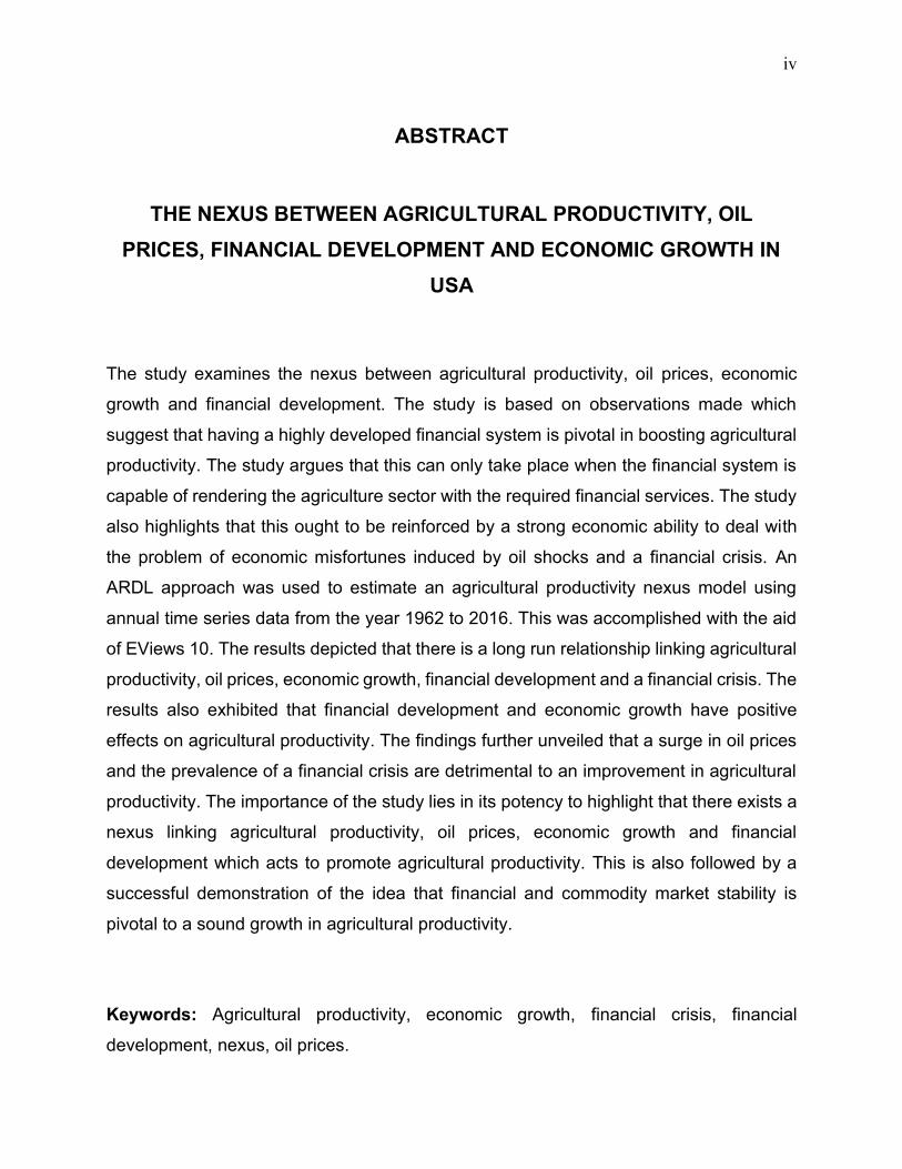
The study examines the nexus between agricultural productivity, oil prices, economic
growth and financial development. The study is based on observations made which
suggest that having a highly developed financial system is pivotal in boosting agricultural
productivity. The study argues that this can only take place when the financial system is
capable of rendering the agriculture sector with the required financial services. The study
also highlights that this ought to be reinforced by a strong economic ability to deal with
the problem of economic misfortunes induced by oil shocks and a financial crisis. An
ARDL approach was used to estimate an agricultural productivity nexus model using
annual time series data from the year 1962 to 2016. This was accomplished with the aid
of EViews 10. The results depicted that there is a long run relationship linking agricultural
productivity, oil prices, economic growth, financial development and a financial crisis. The
results also exhibited that financial development and economic growth have positive
effects on agricultural productivity. The findings further unveiled that a surge in oil prices
and the prevalence of a financial crisis are detrimental to an improvement in agricultural
productivity. The importance of the study lies in its potency to highlight that there exists a
nexus linking agricultural productivity, oil prices, economic growth and financial
development which acts to promote agricultural productivity. This is also followed by a
successful demonstration of the idea that financial and commodity market stability is
pivotal to a sound growth in agricultural productivity.
Keywords: Agricultural productivity, economic growth, financial crisis, financial
development, nexus, oil prices.

v
ŐZ
ABD’DEKİ TARIMSAL VERİMLİLİK, PETROL FİYATLARI, FİNANSAL
KALKINMA VE EKONOMİK BÜYÜME ARASINDAKİ BAĞLANTI
NOKTALARI
Bu çalışma tarımsal verimlilik, petrol fiyatları, ekonomik büyüme ve finansal gelişme
arasındaki bağlantı noktalarını incelemektedir. Çalışma, oldukça gelişmiş bir finansal
sisteme sahip olmanın tarımsal verimliliği artırmada çok önemli olduğunu öne süren
gözlemlere dayanmaktadır.Çalışma, bunun ancak finansal sistemin tarım sektörünü
gerekli finansal hizmetlerle sağlayabilmesi durumunda gerçekleşebileceğini savunuyor.
Çalışma ayrıca bunun petrol şokları ve finansal krizlerin yol açtığı ekonomik talihsizlik
sorunlarıyla başa çıkabilmek için güçlü bir ekonomik yetenekle güçlendirilmesi gerektiğini
vurgulamaktadır. 1962'den 2016'ya kadar yıllık zaman serileri verilerini kullanarak bir
tarımsal verimlilik bağıntısı modelini tahmin etmek için bir ARDL yaklaşımı kullanıldı. Bu,
EViews 10'un yardımı ile başarıldı. Sonuçlar, tarımsal üretkenliği, petrol fiyatlarını,
ekonomik büyümeyi, finansal gelişimi ve finansal bir krizi ilişkilendiren uzun vadeli bir ilişki
olduğunu göstermiştir. Sonuçlar ayrıca finansal kalkınma ve ekonomik büyümenin
tarımsal üretkenliği olumlu yönde etkilediğini göstermiştir. Bulgular ayrıca, petrol
fiyatlarındaki bir artışın ve finansal krizin tarımsal üretkenliğe zarar verdiğini ortaya
koymuştur. Çalışmanın önemi, tarımsal üretkenliği teşvik eden, tarımsal üretkenliği, petrol
fiyatlarını, ekonomik büyümeyi ve finansal kalkınmayı bağlayan bir bağın var olduğunu
vurgulama gücünde yatmaktadır.Bunu, finansal ve emtia piyasası istikrarının tarımsal
üretkenlikte sağlam bir büyüme için çok önemli olduğu fikrinin başarılı bir şekilde
kanıtlanması izlemektedir.
Anahtar Kelimeler: Tarımsal verimlilik, ekonomik büyüme, finansal kriz, finansal
kalkınma, bağlantı noktası, petrol fiyatları.

vi
TABLE OF CONTENTS
ACCEPTANCE
DECLARATION ............................................................................................................... i
DEDICATION .................................................................................................................. ii
ACKNOWLEDGEMENTS .............................................................................................. iii
ABSTRACT ................................................................................................................... iv
ŐZ ................................................................................................................................... v
TABLE OF CONTENTS ................................................................................................. vi
LIST OF FIGURES......................................................................................................... ix
LIST OF TABLES ........................................................................................................... x
ABBREVIATIONS.......................................................................................................... xi
INTRODUCTION ............................................................................................................. 1
CHAPTER ONE .............................................................................................................. 6
LITERATURE REVIEW .................................................................................................. 6
1.1 Introduction ............................................................................................................... 6
1.2 Theoretical insights on agricultural productivity and its drivers .................................. 6
1.2.1 The high payoff input model ................................................................................... 7
1.3 The notion of agricultural productivity ........................................................................ 9
1.3.1 The macro impacts of agricultural growth ............................................................... 9
1.3.2 Agricultural growth spillovers to other sectors ...................................................... 11
1.3.3 Agricultural growth and its impact on poverty ....................................................... 12
1.4 Oil shocks and a plunge in oil prices ....................................................................... 13
1.5 The changing context of economic growth and its drivers ....................................... 15
1.6 The ever-significant role of financial development in modern economics ................ 18
1.7 The ravaging effects of a financial crisis .................................................................. 21
1.8 Empirical studies on agricultural productivity, financial development, oil prices and
economic growth ........................................................................................................... 23
1.8.1 The nexus between agricultural productivity and oil prices .................................. 23
1.8.2 The nexus between agricultural productivity and economic growth...................... 25
1.8.3 The nexus between agricultural productivity and financial development .............. 29

vii
1.8.4 The nexus between agricultural productivity and a financial crisis ....................... 32
1.9 Summary of empirical studies ................................................................................. 35
CHAPTER TWO............................................................................................................ 38
AGRICULTURAL PRODUCTIVITY, OIL PRODUCTION, FINANCIAL DEVELOPMENT
AND ECONOMIC GROWTH INITIATIVES IN THE USA .............................................. 38
2.1 Introduction ............................................................................................................. 38
2.2 Overview of the USA economy ............................................................................... 38
2.3 Agricultural initiatives and programmes ................................................................... 39
2.4 An examination of the USA’s oil production initiatives and effects .......................... 40
2.5 Effects of the 2008 financial crisis on agricultural productivity ................................. 41
2.6 Summary ................................................................................................................. 43
CHAPTER THREE ........................................................................................................ 44
RESEARCH METHODOLOGY ..................................................................................... 44
3.1 Research design ..................................................................................................... 44
3.2 Assumptions ............................................................................................................ 44
3.3 Model estimation techniques ................................................................................... 45
3.4 Model tests .............................................................................................................. 47
3.4.1 Stationarity tests ................................................................................................... 47
3.4.2 Granger causality tests ......................................................................................... 47
3.4.3 Cointegration tests ............................................................................................... 48
3.4.4 Sensitivity analysis ............................................................................................... 49
3.5 Definition of variables and the expected impact ...................................................... 51
3.6 Data sources ........................................................................................................... 52
CHAPTER FOUR .......................................................................................................... 54
DATA ANALYSIS AND PRESENTATION ................................................................... 54
4.1 Unit root tests .......................................................................................................... 54
4.2 Structural break test ................................................................................................ 55
4.3 Correlation coefficient test ....................................................................................... 56
4.4 ARDL Bounds test ................................................................................................... 57
4.4.1 Cointegrating form ................................................................................................ 58
4.4.2 Short run bounds test results................................................................................ 58
viii
4.4.3 Long run bounds test ............................................................................................ 60
4.5 Sensitivity analysis .................................................................................................. 61
4.6 Redundant variable test .......................................................................................... 62
4.7 Stability tests ........................................................................................................... 63
4.8 Model performance and forecast error diagnosis .................................................... 63
4.9 Effects of financial development on agricultural productivity ................................... 64
4.10 Discussion of findings and answers to the research questions ............................. 65
CHAPTER FIVE ............................................................................................................ 70
CONCLUSIONS, POLICY IMPLICATIONS AND SUGGESTIONS FOR FUTURE
RESEARCH .................................................................................................................. 70
5.1 Conclusions ............................................................................................................. 70
5.2 Recommendations .................................................................................................. 72
5.2.1 Recommendations to agricultural players ............................................................ 72
5.2.2 Recommendations to financial institutions ........................................................... 72
5.2.3 Recommendations to the government .................................................................. 73
5.3 Suggestions for future studies ................................................................................. 73
REFERENCES .............................................................................................................. 74
LIST OF APPENDICES ................................................................................................ 85
Appendix I: Chow Breakpoint test ................................................................................. 85
Appendix II: ARDL model estimation ............................................................................. 86
Appendix III: Long run form ........................................................................................... 87
Appendix IV: Error correction regression ....................................................................... 88
Appendix V: Bounds test ............................................................................................... 89
Appendix VI: Log likelihood test .................................................................................... 90
Appendix VII: Ramsey reset .......................................................................................... 91
Appendix VIII: Normality test ......................................................................................... 92
Appendix VIV: Arch Heteroscedasticity test .................................................................. 93
Appendix X: Breusch-Pagan-Godfrey ........................................................................... 94
Appendix XI: Serial correlation LM test ......................................................................... 95
SIMILARITY INDEX ...................................................................................................... 96
ETHICAL APPROVAL .................................................................................................. 97
ix
LIST OF FIGURES
Figure 1.1: Conceptual framework ................................................................... 36
Figure 2.1: Mortgage delinquency rates for USA’s subprime loans .................. 41
Figure 2.2: Externalities from a financial crisis ................................................. 42
Figure 4.1: Cusum stability inquiries ................................................................. 63
Figure 4.2: Model performance and forecast error diagnosis ........................... 64

x
LIST OF TABLES
Table 1.1: Summary of the nexus between agricultural productivity and oil prices 25
Table 1.2: Summary of the nexus between agricultural productivity and economic
growth ............................................................................................................... 28
Table 1.3: Summary of the nexus between agricultural productivity and financial
development ...................................................................................................... 31
Table 1.4: Summary of the nexus between agricultural productivity and a financial
crisis .................................................................................................................. 34
Table 2.1: Overview of the US economy .......................................................... 39
Table 3.1: Definition of variables and expected impact..................................... 51
Table 3.2: Variable description and data source ............................................... 52
Table 3.3: Descriptive statistics in natural form ................................................ 52
Table 3.4: Descriptive statistics in log form ....................................................... 53
Table 4.1: Innovational structural break unit root test ....................................... 54
Table 4.2: Additive structural break unit root test .............................................. 54
Table 4.3: Chow Breakpoint test ....................................................................... 55
Table 4.4: Pearson correlation coefficient test .................................................. 57
Table 4.5: ARDL Cointegration test .................................................................. 58
Table 4.6: Cointegrating form ........................................................................... 58
Table 4.7: Short run bounds test estimations ................................................... 59
Table 4.8: Long run bounds test ....................................................................... 60
Table 4.9: Sensitivity analysis ........................................................................... 62
Table 4.10: Redundant variable test ................................................................. 62
Table 4.11: Pairwise Granger causality test ..................................................... 65
Table 4.12: Summary of the hypothesis tests ................................................... 65

xi
ABBREVIATIONS
ADF: Augmented Dickey-Fuller
AP: Agricultural Productivity
ARDL: Auto Regressive Distributed Lag
DVFC: Dummy Variable for Financial Crisis
ECT: Error Correction Term
EG: Economic Growth
FD: Financial Development
OP: Oil Prices
PP: Phillips Perron
WFP: World Food Program

1
INTRODUCTION
Background of the study
Agriculture used to be the centre of national and global decision making with
organisations such as the United Nations and the World Food Programme
underscoring the need to boost agricultural productivity (Garnett et al., 2013). This
stemmed from ideas which assert that agricultural productivity goes a long way
towards poverty alleviation (Irz, Lin & Thirtle, 2001; Thirtle, Lin & Piesse, 2003). With
more than 9 billion stricken in poverty and in huge need of food, one cannot deny the
need to promote agricultural productivity (Godfray et al., 2010). Onoja (2017)
acknowledges that effort to promote food security can be made possible by promoting
agricultural productivity. On a large note, agricultural productivity is mainly engineered
to foster economic growth and development and its importance in an economy still
remains undoubtedly significant.
It is highly believed agricultural productivity is one of the key strategies that can be
used to attain Millennium Development Goals (MDGs), (McMichael & Schneider,
2011). Diao, Hazell and Thurlow (2010) believe that agricultural productivity is tied to
quite a number of macroeconomic indicators. Such indicators include financial
development, economic growth and stability. This, therefore, highlights the existence
of a nexus linking agricultural productivity, economic growth and financial
development.
Meanwhile, mass production, technological development, cost and productive
efficiency in the agriculture sector are notable factors that influence the productivity of
the agriculture sector. But there are ideas which posit that these factors can be made
available through the provision of financial assistance by the financial market (Rizwan-
ul-Hassan1, 2017; Shahbaz, Shahbaz & Shabbir, 2003). Onoja (2017) concurred with
this idea and asserted that financial players make it feasible for farmers to acquire high
payoff technology. The acquisition of high payoff technology helps to boost agricultural
productivity. Hence, it can be noted that the financial sector plays a pivotal role in
improving agricultural productivity.

2
On the other hand, the oil sector is one of the most lucrative economic sectors an
economy can have and economies such as the United States of America (USA) have
gained a lot from oil production. Oil production has a strong capacity to turn around
both individual and economic fortunes. This is one of the major reasons why people
may shun other sectors such as agriculture in favour of the oil sector. Alternatively,
this implies that the opportunity cost of engaging in agricultural production is the huge
gain that can be made from participating in oil production, selling and distribution. But
challenges can be observed when oil shocks initiate an increase in oil prices. The
agriculture sector together with other economic industry can suffer from an increase
in oil prices (Alihu, 2009; Berument, Ceylan & Dogan, 2010). This strongly provides
an indication of a negative spillover effect linking changes in oil prices and other
economic sectors. Thus, it is imperative to note that there is a linkage between
agricultural productivity, oil prices, economic growth and financial development.
However, studies have of late confined on separating the individual effects of each
macroeconomic variable, yet they combinedly work to affect agricultural productivity.
Such an observation is reputably true in countries such as the USA which is
characterised by tremendous economic growth and financial development levels. As
a result, this research attempts to examine the presence of a nexus connecting
agricultural productivity, oil prices, economic growth and financial development in the
USA.
Problem statement
A sound increase in agricultural productivity requires an effectively functioning
financial system that is capable of providing the agriculture sector with the required
financial services. But in order to accomplish this, the economy must be growing well
and in a strong position to deal with economic misfortunes caused by volatile oil prices
and shocks, and the effects of a financial crisis.

3
Aims of the study
The core aim of this study is centred on establishing the existence of an interaction
linking agricultural productivity, oil prices, economic growth and financial development.
The study will also place focus on attaining the following targets;
• In the case that there exists an interaction, the study will thus seek to determine
how oil prices, economic growth and financial development influence
agricultural productivity.
• To examine if the agriculture sector is in a position to thrive and maintain high
productivity levels in an economy such as the USA, where much of the focus is
devoted towards heavy industrial products such as oil and minerals. If so, then
determine how oil shocks and volatile changes in oil prices affect agricultural
productivity.
• To examine if developments in the US financial sector have been capable of
stimulating agricultural productivity or not. If not, then proceed to examine if any
possible increases in agricultural productivity managed to stir up financial
development in the USA.
• To determine possible policy implications that can be made to promote
agricultural productivity.
Research inquiries
With respect to the aforementioned aims, this study thus, places focus on providing
answers to the following inquiries;
• Is there an interaction between agricultural productivity, oil prices, economic
growth and financial development? If so, then how do oil prices, economic
growth and financial development influence agricultural productivity?
• In an economy such as the USA, where much of the focus is devoted towards
heavy industrial products such as oil and minerals, will the agriculture sector be
in a position to thrive and maintain high productivity levels? If so, then how do
oil shocks and volatile changes in oil prices affect agricultural productivity?
• Have developments in the US financial sector been capable of stimulating
agricultural productivity or not? If not, then did any possible increases in

4
agricultural productivity stirred up financial development in the USA? This
results in the formulation of the following null hypotheses;
• H1: Positive developments in US financial markets did not cause an
improvement in agricultural productivity.
• H2: An increase in agricultural productivity did not necessitate
positive developments in US financial markets.
• What are the possible policy implications that can be made to promote
agricultural productivity?
Relevance of the study
The importance of the study lies in its potency to highlight that there exists a nexus
linking agricultural productivity, oil prices, economic growth and financial development
which acts to promote agricultural productivity. Furthermore, its propositions play a
vital role in the attainment of millennium development goals, increase food security
and alleviate poverty. Of notable effect is its recognition of the importance of financial
and commodity markets stability in fostering agricultural growth, financial development
and economic growth. Also, resolutions presented in this study, go a long way in
assisting policymakers to devise sound financial development and economic growth-
related policies. The research adds to the existing research on agricultural productivity,
oil prices, economic growth and financial development.
Scope of the study
The research confines on the call to examine the nexus linking agricultural productivity,
oil prices, economic growth and financial development. As such, it bases its
examination, arguments and propositions on findings on the United States of America.
The study also relies on the use of annual secondary data from the year 1962 to 2016
to estimate an ARDL model.
Structure of the study
This thesis will initially look at issues surrounding the essence of agricultural
productivity and how it links with macroeconomic variables such as oil prices,

5
economic growth and financial development. Consequently, it identifies and deals with
empirical gaps that have of long remained unaddressed. The second part of the thesis
is devoted to the application of theoretical and empirical frameworks to assist in
examining the nexus linking agricultural productivity, oil prices, economic growth and
financial development. The third chapter provides an overview of agricultural
productivity, oil prices, economic growth and financial development trends, issues,
contributions and developments. The fourth chapter outlines the methodological
approaches that were undertaken to estimate an agricultural productivity nexus model.
The fifth chapter deals with the presentation of findings established from the estimation
process while the final chapter looks at conclusions, recommendations and proposals
tendered from the research.

6
CHAPTER ONE
LITERATURE REVIEW
1.1 Introduction
Academic studies often contradict with each either based on theoretical or empirical
foundations. Thus, theoretical or empirical studies are a base on which a study can
base its defence. This is however not limited to establishing support for established
ideas or arguments but also as a way of identifying theoretical and empirical gaps.
This chapter, therefore, seeks to identify theoretical and empirical gaps surrounding
the existence of a nexus interaction linking agricultural productivity, oil prices,
economic growth and financial development. It is also from these theoretical and
empirical guidelines that discussion of findings will be centred on.
1.2 Theoretical insights on agricultural productivity and its drivers
The nexus between agricultural productivity, financial development, oil prices and
economic growth can be best examined by looking at theories that examine how they
interact with each other. Such an interaction is best illustrated by looking at the
macroeconomic determinants of agricultural productivity. The notable theory that can
best illustrate the required interaction is the high payoff input model. The relevance of
this theory in this study is justified by the fact that it contends that there is a positive
interaction that exists between agriculture growth, economic and financial stability, and
macroeconomic variables. That is, it posits that there is an interdependence between
economic, commodity market and financial stability, and macroeconomic variables
which act to influence agriculture growth. This model is herein examined in details.
7
1.2.1 The high payoff input model
This theory offers an insight into the micro and macroeconomic factors that are
required to boost agricultural productivity. The microeconomic aspects of the theory
are based on the need to improve labour productivity while the macroeconomic
aspects are based on efforts to provide high-payoff technology and other inputs. This
theory thus shows that improvements in agricultural productivity are not solely based
on microeconomic factors such as labour and capital. But rather on the existence of
other external players and institutions which in this case are financial institutions which
provide farmers with funds to acquire high-payoff technology (Udemezue & Osegbue,
2018). Also, research institutions will serve to provide farmers with the necessary
technical and professional know how that is required to engage and boost agriculture
productivity. Efforts to understand how such a theory explains the nexus between
agricultural productivity, oil prices, economic growth and financial development can
also be achieved by looking at the model assumptions. The theory is based on the
following assumptions;
• Economic growth is determined by the availability and affordability of high-
payoff technology.
• Financial investments in the agriculture sector are determined by the ability of
farmers to effectively allocate and use resources.
The first assumption illustrates that there is an interaction that exists between
economic growth and financial development. In the sense that, the financial sector
provides farmers with loans which they use to acquire high-payoff technology.
This, therefore, implies that there is a positive association that exists between
economic growth and financial development. Udemezue and Osegbue (2018)
acknowledge that this assumption helps to explain why there exist differences in
economic growth between poor countries and well-developed economies such as the
United States of America (USA). That is, it contends that poor countries do not have
access to high-payoff technology. As such, their ability to attain a high level of
economic growth depends on their potency to acquire high-payoff technology. This is
contrary to the USA which has a high availability of high-payoff technology and hence
explains why its agriculture sector productivity and growth levels are high. This can
thus be traced to the viability, growth and development of their respective financial

8
sectors. Implying that high growth economies have high agricultural productivity levels
as a result of having well developed financial sectors.
It is also imperative to note that much of the high-payoff technology that is used in the
agriculture sector rely on the use of petroleum products as a source of energy. This
entails that oil shocks will impose severe negative effects on the agriculture sector.
Binuomote and Odeniyi (2013) concurs with the idea and established that the same
happened in Nigeria. If oil prices increase to a severe and unstainable level, they may
trigger a financial crisis in the form of an oil bubble (Sornette, Woodard, & Zhou, 2009).
Hence, it can be noted that stability in the financial and commodity markets is essential
for a sound improvement in agricultural productivity.
The second assumption illustrates that investments in the agriculture sector are
determined by the effective and efficient use of resources in the agriculture sector.
Effective and efficient of resources are thus indicators which investors can utilise to
make investment decisions. This also translates to a decline in non-performing loans
allocated to the agriculture sector by the financial sector (Louzis, Vouldis, & Metaxas,
2012). Meaning that an increase in agricultural productivity improves the ability of
farmers to repay back their agriculture loans leading to a decline in non-performing
loans. Alternatively, banks can be said to benefit profit wise from an improvement in
agricultural productivity.
The major challenge with this theoretical aspect is that it does not offer sound
explanations about the roles played by educational and research institutions.
However, this theory is a close reflection of real economic situations. This is because
it acknowledges the importance and role of the government in influencing economic
activities. It also emphasises the importance of maintaining stability in financial and
commodity markets, and the economy at large. More so, it highlights that economic
growth strategies targeted at improving agricultural productivity through the effective
and efficient use of resources have positive implications for financial development.
This, however, relies on financial, commodity markets and economic stability. This
illustrates the existence of a nexus between agriculture growth, economic and financial
stability, and macroeconomic variables.

9
1.3 The notion of agricultural productivity
Agriculture is one of the core pillars of economic growth and development and its
contribution to economic growth and development is in the form of notable aspects.
Among others, one can contend that agriculture contributes towards improving
domestic incomes (Diao, Hazell & Thurlow, 2010), results in increased food supply
(Onoja, 2017), results in a decrease in the prices of basic foodstuffs (Dercon & Gollin,
2014) etc. however, the capacity of agriculture to institute such effects is largely
determined by the agricultural productivity. Studies often define agricultural
productivity in terms of the total agricultural output that has been produced (Godfray
et al., 2010; Rizwan-ul-Hassan1, 2017). However, agricultural productivity can be
defined in quite a number of ways. For instance, Godfray et al. (2010) defined it as the
capacity of agricultural farmers to produce more output using a given combination of
labour and capital resources. Onoja (2017) defined agricultural productivity as the
interaction between capital and labour inputs to influence agricultural output. However,
in this study, agricultural productivity will be defined based on its capacity to reduce
agricultural imports. This is because the USA has in the past experienced a high rise
in agricultural imports. Hence, determining how agricultural productivity helps to curb
a rise in agricultural imports will be of great essence in this study. Prior to this, an
examination of the macro impacts of agriculture, its spillover effects and impact on
poverty will be discussed in detail.
1.3.1 The macro impacts of agricultural growth
The essence of agriculture has had its contributions towards economic development
recognised way back (Johnston & Miller, 1961). Notable ideas on the importance of
agriculture are based on the assertion that agriculture has positive effects on
consumption and production (Dercon & Gollin, 2014). But much of the impact of
agriculture were assumed to be strictly confined towards assisting and developing
rural communities (Johnston & Miller, 1961). For instance, Yazdani (2008) has in the
past established that agricultural growth causes a simultaneous increase in rural
income. On the other hand,
The importance of agriculture on the economy can also be established by using the
Johnston-Mellor model. The model is based on assertions which pointed out that the
high growth levels observed in Japan and Europe were highly linked to high
agricultural growth levels (Dercon & Gollin, 2014). The World Bank Report (2008)
10
outlined that the early stages of economic growth and development of Sub-Saharan
African economies are highly driven by high agricultural productivity. Moreover, goes
a long way in promoting self-sustainability thereby reducing import expenditure. This
is of paramount importance to less developed economies which might be struggling to
attain high growth standards. This is because most less developed economies will be
having high current account deficit and debts levels (Gollin, Parente & Rogerson,
2002). Hence, expending a lot of resources towards importing agricultural produce will
exacerbate the situation.
It can also be noted that a fall in the prices of agricultural produce will have huge
positive macroeconomic effects on inflation. This is highly true especially when
considerations are made that the prices of foodstuffs, is the notable driver of inflation
(Gollin, Parente & Rogerson, 2004). But the extent to which such an effect will reduce
inflation is highly determined by the extent to which agricultural productivity will drive
down the prices of non-agricultural products.
On a deeper perspective, the problem of high unemployment levels in both less and
highly developed economies can be eased by promoting high agricultural growth and
boosting agricultural productivity. A high number of unemployed individuals are
considered to be residing in rural areas (Gollin, Parente & Rogerson, 2007). Since
agricultural activities are highly concentrated in rural areas, promoting agricultural
growth and productivity will thus help to ease rural unemployment problems.
On a more significant term, agricultural growth and productivity play an important role
in poverty reduction (World Development Report, 2008). With the surging poverty
levels especially in a high number of African countries, it, therefore, remains imperative
that agricultural growth is used to alleviate poverty. This goes a long way in aiding
towards the attainment of Millennium Development Goals (MDGs).
Care must also be placed on noting that improvement in agricultural productivity will
also ease the pressure on international organisations such as the World Food
Programme (WFP) and other international bodies. The WFP and other international
stakeholders work together in dealing with food security challenges in Africa and other
poor countries. Poverty thus places a huge burden on these organisations to provide
food assistance to numerous countries. Hence, by promoting agricultural growth and
productivity will have ripple effects on other international bodies. It can thus be
11
deduced that agriculture growth has positive the effects on third world countries and
international bodies.
1.3.2 Agricultural growth spillovers to other sectors
In relation to the perspective that agriculture has spillover effects on other sectors, it
can easily be summed up that the effects are on non-agriculture sectors. The dominant
paradigm is in Tiffin and Irz (2006) states that agriculture growth has causal effects on
economic growth.
McArthur and Sachs (2013) argue that improvements in agricultural productivity work
towards driving down the prices of food stuffs. This is important because it has
multiplier effects on other sectors. This can be reinforced by Dercon and Gollin (2014)
who contends that a downward spiral of prices of agricultural products results in an
expansion for the market of non-agricultural products. This is because a significant
number of non-agricultural products and services are complementary to agriculture
products. In addition, this will result in an improvement in the competitiveness of non-
agricultural products.
There are also ideas which suggest that the growth of other sectors also tied to
agricultural growth (Fan et al., 2000). This can be attributed that agricultural output
forms an input in other sectors. Hence, a growth in the supply of agricultural produce
will boost the supplier of resources into these sectors. Ultimately, the price of factor
inputs into these sectors will fall and resource supply will increase leading to an
increase in productivity. It is thus, in this regard that agriculture is considered to be
having spillover effects.
On the other hand, investors often look at agricultural trends and how other sectors
are performing in relation to changes in agricultural trends. As such, observations
made by Fan et al. (2000) will thus help to explain why other sectors witness increases
in investment levels following a growth in agriculture.
Another perspective from which agricultural spillover effects can be examined is in
terms of backward and forward supply mechanisms. Block (1999) posits that industries
which supply agriculture with resources will also benefit from agriculture growth and
productivity.
12
He challenges with ideas concerning the simultaneous and endogeneity effects of a
growth in agriculture is lack of empirical support. This is because the idea of agriculture
having multiplier effects on other sectors is very subjective. For instance, a growth in
other sectors might also be linked to a growth in other sectors which are separate from
agriculture. In some cases, the growth in other sectors might be tied to unnoticeable
changes in other different sectors. This is because there are certain changes or effects
that are difficult to notice but yet they have notable effects on other indicators (Dercon
& Gollin, 2014). The size of the multiplier effects also difficult to determine. Hence,
conclusions can be made in respect of this argument that there is a need for
considerable research to examine the spillover effects of a growth in agriculture.
1.3.3 Agricultural growth and its impact on poverty
The implications of agricultural productivity on poverty reduced are mainly centred on
the notion at a lot of individuals obtain their income from agricultural activities (Diao,
Hazell & Thurlow, 2010). A lot of individuals assume that promoting agricultural growth
and development will result in farmers getting a lot of income from farming activities
(Christiaensen Demery & Kuhl, 2011; Ravallion & Chen, 2007; Stifel & Thorbecke,
2003). By doing so, income growth from farming activities can thus be used as a
means of sustaining lives. Apart from that, there are also nutritional and food security
benefits that are associated with agricultural growth and development. All in all, these
benefits act together to alleviate poverty
Despite the existence of ideas which contend that agriculture growth helps to alleviate
poverty there are conditions to which such an idea will hold. For instance, Stifel and
Thorbecke (2003) acknowledge that agriculture growth will cause a significant
reduction in poverty on the condition that prices of agricultural produce either remain
constant or increase. This is because a downward change in the price of agricultural
produce will necessitate a reduction in farmers’ disposal incomes. It is against this
background that one can dismiss that agriculture has positive implications on poverty
alleviation.
With a growing concern that land for agricultural production is declining on a surging
rate, arguments can thus be levelled that the impact of agriculture growth on poverty
is constrained (Ligon & Sadoulet, 2008). This accompanied by a growth in
industrialisation and a high number of infrastructural development projects, notably

13
real estate, have been at the expense of agricultural growth. Under such a scenario,
it becomes a daunting task to use agricultural growth and development as a strategy
for tackling problems such as poverty and unemployment.
Also, the relationship between agriculture growth and poverty hinges on the
distribution of poverty levels (Christiaensen Demery & Kuhl, 2011). That is, poverty
levels are in most cases high is less developed countries as posed to developed
countries. This implies that the impact of agriculture growth is more likely to be
distributed unequally. For example, one cannot expect an increase in agriculture
growth in Africa to have the same reduction effects on poverty in the USA. This also
influenced by a series of economic activities such as industrialisation, financial and
economic development etc. Ravallion and Chen (2007) echoed the same sentiments
and established that the effects of agriculture growth are 4 times higher than those of
non-agriculture-based economies.
Lastly, differences can also be observed between what may be interpreted as cause
and effect. That is, the impact of agriculture growth on poverty is often interpreted in
the form of elastic responses (Dercon & Gollin, 2014). As a such, the positive
implication of agriculture growth does not entail that the relevant strategy will be in
favour of agricultural investment.
1.4 Oil shocks and a plunge in oil prices
Foremost, the impact of oil prices on any economy is in most cases determined by
whether the country is an oil-producing economy or not. That is, oil producing
economies will to some relative extent benefit from an increase in oil prices through
increased foreign currency inflows (Mohaddes & Pesaran, 2017). However, this must
be weighed against the impact of changes in oil prices on other macroeconomic
variables. Bernanke (2016) agrees with this idea and contends that it is not every oil
producing economy that benefits from an increase in oil prices. Such differences are
attributed to structural and economic differences between oil producing economies.
Hence, this can pose effects on the examination of the nexus between oil prices and
other macroeconomic variables. This, therefore, serves as one of the secondary aims
and significance of this study. As a result, the study seeks to examine how structural
and economic conditions in the USA influence nexus between oil prices and other

14
macroeconomic variables. This, however, requires a deeper understanding of what
drives oil prices and examining possible changes in oil prices that have taken place in
the past years. This leads to two important aspects of oil shocks and a plunge in oil
prices.
Oil shocks are in most cases the main cause of an oil crisis and a sudden upward
spiral in oil prices that is accompanied by a reduction in oil supply is known as an oil
crisis (Obstfeld et al., 2016). Under normal circumstance, an increase in oil prices
poses severe negative effects on the global economy. This is because oil serves as a
major source of energy and hence disruptions in supply caused by high prices will
affect both global production and consumption activities.
The first oil crisis took place in the year 1973 following efforts by OPEC members from
the Arab community to hike oil prices 4 times to US$12/barrel (Bernanke, 2016). This
had severe effects on highly industrialised economies such as those in Europe
including Japan and the USA. It is estimated that global oil consumption in Europe
including Japan and the USA accounts for more than 50% of the world’s energy
(Obstfeld et al. 2016). This problem was further compounded by the fact that exports
to these three major oil consuming nations were being restricted from the onset of the
crisis (Chudik & Pesaran, 2016). The 1973 oil crisis was significantly blamed on the
falling value of the US dollar which is the denominated currency for oil sales. But the
resultant effect was a recession which was followed by inflation. Efforts were made to
restructure the affected economies as fears grew that a high dependency on oil
production would further plunge economies into a doldrum.
The second oil crisis took place in 1979 following the occurrence of the Iranian
revolution which led to severe destruction of Iran’s oil industry. This was further
compounded by the Iraq-Iraq war which took place between the period 1980 to 1988
(Chudik & Pesaran, 2016). During this period the price of oil went up to US$32/barrel
(Mohaddes & Pesaran, 2017).
In spite of the 1973 and 1979 oil crises which drove prices up, the plunge of oil prices
in 2016 had stern downward effects on oil prices. In 2016, the price of oil went down
to US$35/barrel from US$115/barrel in 2014 (Kilian, 2014). The drop-in oil prices were
much attributed to a supply glut. That is, too much oil being supplied on the market
way much more than what the market could handle and this was against falling

15
demand for oil. The plunge in oil prices had contagion effects on the financial sector
and the prices of most commodities started going down. in addition, most non-oil
producing economies suffered a decline in export levels as oil-producing countries
started cutting down their import expenditure. This is because much of the exports
from oil-producing economies such as Iraq and USA were mainly financed by oil
revenue (Kilian, 2014).
From these observations, it is therefore imperative to note that changes in oil prices
are either as a result of a crisis that drives prices up or a plunge in oil prices. The
effects of these two scenarios on economies are totally different. Hence, in some
cases, a unilateral relationship between changes in oil prices and other economic
variables can be observed while in other cases the opposite is true. This can be
supported from insights obtained from a study by Mohaddes and Pesaran (2017)
which exhibited that there is a negative association between oil prices and economic
growth. However, contrasting observations were made by Nazir (2015) who
established that there is a unilateral association between oil prices and economic
growth in the short run. Hence, much of the long-term policies should be centred on
hedging against the effects of rising oil prices. Considerations must be placed also to
notice that the effects of changes in oil prices also poses effects on a significant
number of macroeconomic variables. This can thus assist in identifying and outlining
the possible nexus that exists between oil prices and macroeconomic variables.
1.5 The changing context of economic growth and its drivers
Economic growth is one of the most essential topics in national and global economics
and much of the problems and economic gains are being attributed to variations in
economic growth (Bouis, Duval & Murtin, 2011). With gross domestic product (GDP)
serving as an indicator of economic performance, economic policymakers usually
devote significant effort towards maintaining growth levels above sustainable levels.
Failure by economic agents to maintain GDP growth levels above these sustainable
levels can have disastrous effects on an economy. For instance, a recession is widely
believed to be an indicator of economic failure by the government to stir the economic
towards the desired path (Warr & Ayres, 2012).
16
It is worthy to note also that economic performance is also an indicator of economic
development and this is what is separating rich economies from poor economies.
Moreover, it is the desire of any economy to attain high growth levels at all costs.
However, the global economy has gone through a lot of periods of numerous and
significant changes. As a result, what is currently driving economic growth nowadays
is totally different from what used to stir growth in the past 40 years. Such changes
have been observed to be either posing severe challenges on other economies
especially less developed economies (Kramin et al., 2014). On the other hand, highly
developed economies seem to have gotten better in the midst of these changes (Dao,
2014).
Successful policies designed to stir economic growth and development can thus be
effective when governments are fully aware of the prevailing major drivers of economic
growth. For instance, Fatas and Mihov (2009) discovered that more than 70% of the
world output is being produced by rich economies. Fatas and Mihov further contended
that such as an ability to dominate in terms of global output production is what is
causing rich economies to become richer (2009, p.1). Thus, if poor economies are to
learn from rich economies, then an examination is needed to look at major drivers of
economic growth in rich and well-developed economies.
Meanwhile, the USA has risen significantly as an economic powerhouse followed by
China and their share of the world output is assumed to have exceeded 50% in 2015
(Fatas & Mihov, 2009). The changing context of economic growth and its drivers has
mainly driven by four aspects and these aspects are;
• Innovation: Innovation is much linked to new products and technology but in
reality, it goes beyond developing new products and technology. Vella (2018)
echoed the same sentiments and established that innovation mainly deals with
the development of new ways of producing commodities and delivery services.
That is, coming up with better organisation, production and management
methods. Innovation is also linked to productive and technical efficiency (Fatas
& Mihov, 2009). The more economies produce (mass production) at a lower
cost (productive efficiency), the more resources will be expended towards the
production of other commodities. Hence, highly innovative economies such as
the USA are in a strong position to expend more resources to the production of
17
other commodities as a result of innovation. This also results in an increase in
foreign currency inflows as more output is exported at lower prices. The
domestic economy benefits a lot from a reduction in domestic prices
(disinflationary effects) and income growth.
• Investment: Investment is a key catalyst to economic growth and development
and this is one of the main reasons why countries around the world desire to
lure foreign direct investments. This can be supported by observations made
by Fatas and Mihov, (2009) which exhibited that economic convergence and
divergence as a result of differences in investment levels. That is, it is believed
by Kramin et al. (2014) that economies that are in a position to secure
investment will converge at the same rate as the USA and other G7 economies
(2009, p.7). this implies that economies that cannot access the required
investment level will diverge and become poorer. Such an observation can thus
aid in explaining differences in economic growth and development between rich
and poor economies. A growth in investment can thus, be said to act in favour
of economic growth and development. But the effective distribution of
investment funds requires that the financial sector be well-developed. This
brings us to the third driver of economic growth.
• Institutional environment: The institutional environment must be conducive
for both private and public corporations to undertake production activities. Much
of the challenges that hinder economic growth are as a result of a volatile
macroeconomic environment that makes it difficult for corporations to thrive
(Bouis, Duval & Murtin, 2011). A conducive institutional environment thus
requires that governmental institutions be capable of fostering macroeconomic
stability. This can be accomplished by providing incentives for economic
players to foster stability. But a notable role must be played by the government
through enacting policies, rules and regulations that encourage transparency,
technological innovation, efficiency and human capital investment and
development. Bouis, Duval and Murtin (2011) further outlined that the other key
strategy that can be used to foster institutional stability is promoting financial
development (Vella, 2018). This is because financial institutions work towards
providing the much-needed funds to support production and consumption
activities. This strategy thus links economic growth to financial development

18
and the interaction of these two aspects can also be linked to other economic
indicators such as agricultural productivity and dealing with the effects of oil
changes in oil prices. Institutional stability also extends to include how
government deal with economic catastrophes such as a financial crisis. Inability
to deal with economic challenges such as oil shocks and financial crisis can
thus be seen as affecting a wide number of economic indicators. This,
therefore, leads us back to the idea of a nexus between agricultural productivity,
oil prices, economic growth and financial development and incorporating the
effects of a financial crisis.
• Initial conditions: There is an idea that initial economic conditions are a major
determinant of future growth potential (Dao, 2014). Warr and Ayres (2012) also
shared the same sentiments and expressed that either initial convergence or
divergence conditions will provide a strong indication of an economy’s growth
potential. That is, poor countries will be capable of growing faster when they
are aligned to convergence patterns of well-developed economies. The same
applies to rich economies and their prospects and determined by their ability to
remain on a convergence path.
Using ideas derived from the given drivers of economic growth, it can be noted that
innovation is required to stir both financial and economic growth and development. But
efforts to attain high levels of economic performance (high GDP levels) are determined
by the availability of investment funds. Of which the effective distribution of investment
funds requires that the financial sector be well developed to source and distribute
funds. All these activities must be done in an economic environment that is free from
economic misfortunes posed by oil shocks and financial crises. In conclusion, these
aspects can thus be said to be illustrating that economic activities do not act
independently of each other but rather interact together in the form of a nexus.
1.6 The ever-significant role of financial development in modern economics
The notion of financial development revolves around the need to execute transactions,
enforce contracts and the existence of information costs (Merton & Bodie, 2004).
These three elements work together towards making it difficult for economic players
19
to engage in consumption and production activities. As a result, financial development
is thus meant to deal with the problems posed by the need to execute transactions,
enforce contracts and the existence of information costs. The resultant effect of such
efforts is the emergence of financial intermediaries, markets and legal systems
(Jorgenson, 2005). Thus, any financial development strategies that incorporate these
aspects together will significantly have an important bearing on economic outcomes.
For instance, the setting up of financial institutions to offer information about market
activities will certainly affect credit provision. On the other hand, things like financial
contracts serve as an assurance that investors are guaranteed to recoup their
investments from investments made in other businesses. But the roles played by
financial institutions also extended to include the provisions of facilities that allow
customers to deposits their savings with banking institutions (Morales, 2003).
Acemoglu, Aghion, and Zilibotti (2003) also acknowledged that the role of financial
institutions is to facilitate investments between firms and investors.
The above-given details on financial development can help to assist in defining
financial development. Financial development can thus be defined as the use of
financial instruments by financial intermediaries on financial markets with the sole aim
of dealing with information and transaction costs. It is from this definition that we can
establish the roles of financial institutions in an economy. These roles help in
examining the nexus between financial development and other macroeconomic
variables.
• Mobilize and pool savings: Deposit-taking institutions normally thrive on
deposit made by customers in the form of savings. The existence of information
and transactions costs make it feasible for individuals and corporations to save
their funds with financial institutions. Banks will intron use those savings to
issue loans to other individuals and corporations in need of funds. When related
to agricultural productivity, it can thus be established that banks help farmers
to acquire agricultural inputs by either securing loans and other financing
options. Banks will generate revenue by levying interest rates and service fees
on loans issued to customers. As a result, an increase in savings is positively
related to bank profitability (Morck, Wolfenzon & Yeung, 2005).
• Facilitate trading, diversification, and management of risk: A significant
number of the roles of financial institutions are linked to the need by financial

20
institutions to provide funds, economic agents. Boyd and Smith (1992) also
concur with this idea and outlined that activities such as trade can be an
expense to undertake due to shortages of funds. Financial institutions,
therefore, serve as a source of funds. This can prove to be too handy especially
in the trading of agricultural products which has to be done across different
geographical boundaries. In addition, banks can issue securities which
individual farmers and other economic agents can use to diversify their
investments (Acemoglu & Zilibotti, 1997). This is of paramount importance,
especially when considering that commodities and other investments can suffer
losses.
• Monitoring investments and enforcing good corporate governance
standards: The existence of financial institutions is primarily centred on the
need to assist economic agents in securing funds either to finance consumption
or production activities. However, the extent to which banks will allocate funds
to individuals and institutions hinges on credit risk. That is the risk profile of the
respondents. Different individual and corporations have different risk profiles
and banks must first assess the creditworthiness of the financial recipient
before granting funds (Wurgler (2000). In doing so, banks therefore directly
monitor and influence the use of funds and this imposes effects on savings and
the allocation of funds. Also, banks are obligated by creditors and investors to
maximise firm value and this causes banks to initiate measures to improve bank
efficiency (Morales, 2003). This causes banks to institute good corporate
governance practices. Failure to do so can cause to lose on the supply of credit
and investment funds. Hence, banks help to monitor funds and enforce good
corporate governance standards.
• Allocating capital and provide investments information: The existence of
financial institutions is in contrary to the assumption of the theory of perfect
competition which assumes that there is perfection information (Morck,
Wolfenzon & Yeung, 2005). In reality, this does not hold and it can actually be
noted that there exists some level of information asymmetry. The problem of
information asymmetry always manifests itself in the form of information and
search costs and such costs can be exorbitant for firms to handle. It is important
to note that savers are reluctant to save when they lack the necessary
21
information and the same applies to investors. Hence, if savers and investors
are to make sound decisions, then they must first acquire and process the
necessary information. But the challenge is that acquiring and processing
information can be costly and time-consuming (Caprio & Levine, 2002). Such
costs and time lost acquiring and processing information can thus be reduced
by involving financial institutions. By providing information at a relatively low
cost, financial institutions can thus assist firms and individuals to make rational
decisions. In doing so, they will thus improve the allocation of resources among
economic activities. As noted from a study by Wurgler (2000), the efficient
allocation of resources in an economy is positively linked to upwards changes
in economic growth. The ability of financial institutions to allocate funds among
productive sectors of the economy and to rational individuals is also positively
related to economic growth. This, therefore, illustrates that there is a positive
interaction that exists between financial development and economic growth.
1.7 The ravaging effects of a financial crisis
One of the notable misfortunes that can affect an economy is a crisis. In economic
terms, there are two notable terms that can be used to describe a crisis. That is an
economic crisis and a financial crisis. The major difference between the two types of
crises is that a financial crisis is mainly characterised by a series of shocks in the
financial markets which lead to a decline in the value of asset prices and increased
insolvency among financial players (Burger et al., 2009). The discrepancy is usually in
the form of disturbances in the allocation of capital. It is imperative to note that there
four different types of financial crises. A financial crisis can either be in the form of a
situation where the government is stuck in a huge debt situation (Debt crisis), (Puri,
Rocholl & Rocholl, 2011). Campello, Graham and Harvey (2010) also outlined that an
economy can be stuck in a situation which is characterised by a sudden stop in current
account inflows (sudden stop). A financial crisis can also be in the form of a bank run.
Hurd and Rohewedder (2010) characterised a bank run as a situation in which panic
behaviour among bank customers causes them to continuously withdraw a lot of funds
from banks. A financial crisis can also be in the form of a foreign currency crisis which
involves a continuous decline in the value of a currency (Song & Lee, 2012).

22
Irrespective of the type of a financial crisis that may be prevalent in an economy, it is
undoubtedly that a financial crisis imposes severe repercussions on an economy.
Such effects are not limited to economic conditions but also extend to include social
repercussions. For instance, Song and Lee (2012) hinted that investment levels
usually drop down significantly in economies affected by a financial crisis. Nobi et al.
(2014) concurs with this idea and contends such effects are attributed to a decline in
productivity levels. Due to disruptions in the allocation of capital, most firms usually
find it difficult to sustain operations when experiencing a financial crisis. All these
effects always connect together leading to a huge decline in economic performance.
That is, economic growth levels are bound to plummet as the financial crisis prolongs
its duration. This is one of the most severe economic effects of a financial crisis.
Economic downturns will hinder the economy in several ways as the ripple effects of
a financial crisis spread to other economic sectors. One can also point out that real
incomes tend to fall during the midst of a financial crisis (Allen, 2011). This can be
attributed to the fact that a financial crisis is associated with a sudden increase in
prices (inflation), (Aloui, Aissa & Nguyen, 2011). If not contained, then the problem of
income inequality is more likely to take effect in the affected economy. This may, in
the long run, lead to increased poverty. Furthermore, numerous individuals can also
lose their jobs and leading to a surge in the unemployment rate. At this stage,
policymakers and individual members would be seeking a quick remedy to get out of
the crisis. Failure to do so will cause social unrests and political instability.
Observations can thus be made that a financial crisis is not a good economic
phenomenon and that its occurrence poses stiff economic and social repercussions.
Though a financial crisis is usually associated with a decline in asset prices, its effects
also spread to affect a lot of economic indicators such productivity, economic
performance, investment, unemployment, poverty, development, human
development. This, therefore, entails that the effects of a financial crisis are not limited
to the financial sector but will also spread to affect the agriculture sector. Such an
ability to affect another economic sector can thus be said to be a nexus. Hence, it can
be concluded under this section that the prevalence of a financial crisis has its effects
linked to other economic sectors.

23
1.8 Empirical studies on agricultural productivity, financial development, oil
prices and economic growth
A decomposition of the nexus between agricultural productivity, financial development,
oil prices and economic growth helps to shed a light on how these variables interact
together. Thus, empirical examinations were made in relation to how financial
development, oil prices economic growth and a financial crisis individually interact with
agricultural productivity.
1.8.1 The nexus between agricultural productivity and oil prices
Olomola and Adejumo (2006) established that oil price shocks have an impact on
macroeconomic activities. Their results were based on the application cointegration
and Variance decomposition in Nigeria suing data from 1970 to 2003. The findings
revealed that there is cointegration linking oil prices with agricultural productivity. This
entails that oil shocks will pose huge effects on the USA’ agriculture sector. In addition,
the study also established that an increase in oil prices will result in a decline in
agriculture’s industrial production index. Hence, it can be expected that an increase in
oil prices will reduce the USA’s agricultural productivity.
Nazlioglu and Soytas (2012) used cointegration and causality to determine the
existence of a nexus linking oil prices and agricultural commodity prices. Based on the
established cointegration results, it was discovered that an increase in oil prices
causes an increase in the price of agricultural products. The results also showed that
the depreciation of the US dollars makes it cheaper to buy agricultural products. This
therefore serves as confirmation that an increase in oil prices results in an increase in
agricultural costs. Such costs are either in the form of input and transportation costs.
The fact that the value of the US dollar determined the price of agricultural products
entails that there is always a nexus that that links agricultural productivity with
macroeconomic variables.
Binuomote and Odeniyi (2013) used a VECM in the contextual situation of Nigeria to
examine the implications of changes in crude oil price on agricultural productivity. Their
study concedes that the increase in crude oil prices has ripple effects on other
economic indicators such as the size of land, quantity of labour and exchange rate.
The established results reinforce that volatile increases in crude oil prices tend to

24
hinder agriculture productivity. Hence, we can expect a similar effect in the context of
USA.
Wang and McPhail (2014) concentrated on the use of a structural VAR to examine
how energy shocks affect US agricultural productivity growth and commodity prices. it
was discovered from their study that energy shocks can be classified as either supply
or demand shocks. This entails that the impact of energy shocks is determined by the
type of energy shocks prevalent in the economy. In such a case, it infers that the
impact of oil prices will also vary with the type of oil shocks affecting the economy.
This can be reinforced by their established results which provided evidence of the
existence of an inverse association between oil prices and productivity.
McFarlane (2016) used a VECM to analyse the effect of oil prices on agricultural
productivity in USA during the period 1999-2005 and 2006-2012. The results are in
strong support of the existence of cointegration linking oil prices with agricultural
productivity. However, the strength of the linkage varies with the period under
consideration. This implies that time periods that are characterised with structural
breaks such as oil shocks and financial crises tend to experience a different nexus.
Hence, expectations are that the financial crisis experienced in USA will pose diverse
and severe effects on agricultural productivity.

25
Table 2.1: Summary of the nexus between agricultural productivity and oil prices
Study Methodology Variables Findings
Olomola and
Adejumo
(2006)
Cointegration
and Variance
decomposition,
Nigeria
(1970-2003)
Consumer price index,
price level, industrial
production index, real
GDP
Consumer Price Index, price
level, real GDP and
agriculture Industrial
Production Index are
cointegrated in the long run.
Nazlioglu and
Soytas (2012)
Cointegration
and causality
(January 1980-
February
2010)
Oil prices, agricultural
commodity prices, US
exchange rate
Negative relationship
between exchange rate and
agricultural prices. Positive
relationship between
agricultural prices and oil
prices
Binuomote and
Odeniyi
(2013).
VECM, Nigeria
(1981-2010)
Amount of fertilizer, size
of land, quantity of
labour, the price of
crude oil, exchange rate
and gross domestic
product from the
agriculture sector.
Oil prices have negative
effects on agricultural
productivity. The amount of
fertilizer, size of land, the
quantity of labour and
exchange rate are positively
related to agricultural
productivity.
Wang and
McPhail (2014)
Structural
VAR, USA
(1948-2011)
Productivity growth,
commodity price and
energy price.
Energy shocks can be
classified as either supply or
demand shocks. The impact
of oil prices will also vary with
the type of oil shocks
affecting the economy.
McFarlane
(2016)
VECM, USA
(1999-2005
and 2006-
2012)
Agricultural productivity
and oil prices
Strong cointegration in the
first period and weak
cointegration in the second
period
1.8.2 The nexus between agricultural productivity and economic growth.
Gunawardena (2012) used a CGE model to analyse the effects of agricultural
productivity on the Sri Lankan economy. Gunawardena argued that the effects of

26
agricultural productivity on economic growth are transmitted through productivity,
prices, and employment. The variables provide insights that both micro and
macroeconomic variables have important implications on agricultural productivity. This
was reinforced by the established results which showed that agricultural productivity
and employment have positive effects on economic growth.
Amone (2014) did a study that focused on proving that agricultural productivity has
effects on quite a number of macroeconomic indicators. As a result, Amone
established that agricultural productivity causes positively changes in employment,
food security, poverty alleviation, economic growth and human development. This
provides support that improvements in agricultural productivity will help to stir
economic growth and development. Hence, we can expect a similar effect in USA.
Amone also established that the relationship between Agricultural productivity and
economic growth is a two-way relationship. This implies that efforts to promote
economic growth will also cause an increase in agricultural productivity.
Ismail and Kabuga (2016) used a VECM to test the effects of agricultural productivity
on economic growth in Nigeria from the period 1986 to 2015. The study managed to
establish the existence of cointegration among agricultural output, economic growth
and labour force. It was also established that positive developments in the labour and
agriculture markets will lead to an increase in economic growth. This suggest the
importance of the need to instil institutional stability in the economy. Arguments of our
study are based on the need to prove that economic growth can also cause an
increase in agricultural productivity.
Awoyemi, Afolabi and Akomolafe (2017) did an impact analysis between agricultural
productivity and economic growth in Nigeria using an ECM approach. The study
mainly argued that a significant variation in agricultural productivity is mainly
influenced by microeconomic indicators. The study established that economic growth
is positively cointegrated with agricultural value added, agricultural labour productivity
and agricultural productivity. However, our arguments are based on the idea that
agricultural productivity is also determined by the interaction between macroeconomic
variables. This study thus seeks to prove that that agricultural productivity is also
determined by the interaction between macroeconomic variables.

27
Amire (2016) incorporated both micro and macroeconomic determinants of agricultural
productivity on economic growth using an OLS approach and time series date from
1981 to 2015. The study argued that the effective contribution of the agriculture sector
on economic growth is determined by the influence of both micro and macroeconomic
determinants of agricultural productivity. This therefore reinforces the importance of
the financial sector in providing funds to acquire high input payoff technology. In
addition, GDP can be said to increase on the condition that there is an effective use
of agricultural resources.
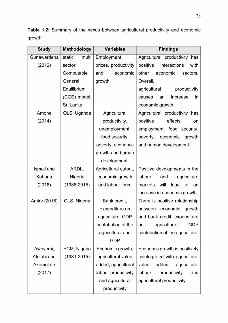
28
Table 1.2: Summary of the nexus between agricultural productivity and economic
growth
Study Methodology Variables Findings
Gunawardena
(2012)
static multi
sector
Computable
General
Equilibrium
(CGE) model,
Sri Lanka
Employment,
prices, productivity
and economic
growth.
Agricultural productivity has
positive interactions with
other economic sectors.
Overall,
agricultural productivity
causes an increase in
economic growth.
Amone
(2014)
OLS, Uganda Agricultural
productivity,
unemployment,
food security,
poverty, economic
growth and human
development.
Agricultural productivity has
positive effects on
employment, food security,
poverty, economic growth
and human development.
Ismail and
Kabuga
(2016)
ARDL,
Nigeria
(1986-2015)
Agricultural output,
economic growth
and labour force
Positive developments in the
labour and agriculture
markets will lead to an
increase in economic growth.
Amire (2016) OLS, Nigeria Bank credit,
expenditure on
agriculture, GDP
contribution of the
agricultural and
GDP
There is positive relationship
between economic growth
and bank credit, expenditure
on agriculture, GDP
contribution of the agricultural
Awoyemi,
Afolabi and
Akomolafe
(2017)
ECM, Nigeria
(1981-2015)
Economic growth,
agricultural value
added, agricultural
labour productivity
and agricultural
productivity
Economic growth is positively
cointegrated with agricultural
value added, agricultural
labour productivity and
agricultural productivity.

29
1.8.3 The nexus between agricultural productivity and financial development
Yazdani (2008) applied a VAR model on data ranging from the year 1979 to 2005 to
examine the interaction between financial market development and agricultural
economic growth in Iran. The results exhibited that trade, growth, interest rate, capital
formation, financial development have a significant impact on agriculture growth.
Muhammad Adnan and Wizarat (2011) did a study that looks at the impact of financial
liberalization on agricultural growth in Pakistan using an ARDL model. It was
established that there is a long run cointegration between financial liberalization index,
real interest rates and agricultural productivity. The results also showed that a long run
increase in real interest rates has a negative effect on agricultural productivity. This
entails that the financial sector can only cause positive developments in the agriculture
sector provided that the change favours agricultural productivity. This serves as a point
upon which positive implications of financial development on agricultural productivity
can be dismissed.
Asghar and Chughtai (2012) applied the OLS regression model to analyse the impact
of providing agricultural credit on the production of wheat in Pakistan. Significant focus
was placed on the role played by microeconomic variables such as pesticide, fertiliser
and agriculture seed. The estimation process also included efforts to examine how
providing credit to farmers helps to enhance farm productivity. The study provided
strong arguments that an effective use of farming resources requires an equitable
provision of capital funding. Hence, it is always important to ensure that farmers have
access to the required lines of credit.
Shahbaz et al. (2013) used an ARDL model to examine how financial development
affects agricultural growth in Pakistan. Using an ARDL model on time series data from
the year 1971-2011, the results established that there exist long-run cointegration
between labour, capital, financial development and agriculture growth. The results also
reinforced the argument that financial development has positive effects on agriculture
growth. Hence, expectations can be made that the highly developed US financial
sector will stir huge positive effects on agricultural productivity.
Dhrifi (2014) focused on examining the effects of financial development on agriculture
on 44 African countries using a GMM panel data estimation approach. Dhrifi argues
that the effects of financial development on agriculture vary with the continent. As a

30
such, the results illustrated that financial development has no positive implications on
agricultural productivity in African countries. This implies that financial development is
more likely to have positive implications for agriculture in the USA. This is because the
USA has a well-developed financial sector that is capable of providing the agriculture
sector with the required funds and services at affordable rates. The study also
contends that the effective functioning of financial institutions is of paramount
importance to the growth and productivity of the agriculture sector. This implies that
anything such as a financial crisis and oil shocks that can hinder financial development
will hinder agricultural productivity and economic growth.
Rizwan-ul-Hassan (2017) used a VAR model to analyse the influence of agricultural
development in Pakistan from the year 1981 to 2015. The results illustrate that the
interaction between agriculture growth and financial development requires positive
changes in financial access, capital and labour. The results, therefore, provide strong
evidence of the essential role of financial development in stirring agricultural
productivity.

31
Table 1.3: Summary of the nexus between agricultural productivity and financial
development
Study Methodology Variables Findings
Shahbaz et
al. (2013)
ARDL model
in Pakistan
(1971-2011)
Labour, capital,
financial development
and agriculture
growth.
Long run cointegration between
Labour, capital, financial
development and agriculture growth.
Financial development has positive
effects on agriculture growth.
Dhrifi
(2014)
GMM on 44
African
countries
(1990-2012)
Technological
innovation,
institutional quality,
financial development
and agriculture
productivity
Financial development has no
positive implications on agricultural
productivity in African countries.
Rizwan-ul-
Hassan
(2017)
VAR model in
Pakistan
(1981-2015)
Agriculture growth,
financial access,
financial
development, capital,
labour.
Positive association between
agriculture growth and financial
access, financial development.
Positive association between
agriculture growth and labour.
Yazdani
(2008)
VAR model in
Iran
(1979-2005)
Trade, growth,
interest rate, capital
formation, financial
development, and real
per capita formation
GDP
Trade, growth, interest rate, capital
formation and financial development
have a significant impact on
agriculture growth.
Asghar and
Chughtai
(2012)
OLS in
Pakistan
Pesticide, fertiliser,
seed and credit to
farmers
Pesticide, fertiliser, seed and credit to
farmers are positively related to
agricultural productivity.
Muhammad
Adnan and
Wizarat
(2011)
ARDL model
in Pakistan
Financial liberalization
index, real interest
rates and agricultural
productivity.
Long run cointegration between
financial liberalization index, real
interest rates and agricultural
productivity. A long run increase in
real interest rates has a negative
effect on agricultural productivity.
32
1.8.4 The nexus between agricultural productivity and a financial crisis
Coyle et al. (1998) conducted an examination of the impact of how the Asian crisis
affects the U.S. Agriculture. Much of the arguments were based on ideas that a
financial crisis disturbs the distribution of credit to the agriculture sector. The challenge
also occurs when the prices of factor inputs increases and this tends to cause an
increase in production costs. This implies that there is a greater need to deal with high
input costs.
Shane and Liefert (2000) did a study that examines the possible existence of
relationship linking a financial crisis to agriculture. The study established that a
financial crisis has linkages that are connected to interest rates, GDP growth and
exchange rate. These linkages were considered to cause changes in agricultural
exports and imports. But these are not the only macroeconomic linkages that exist.
Shane and Liefert also acknowledge this and consider that care must be placed at
examining the existence of other macroeconomic variables. Hence, their study serves
as a base upon which study is based. That is, to examine the existence of linkages
between agricultural productivity and other macroeconomic indicators.
Dia and Roe (2000) did a qualitative analysis of the impact of the financial crisis on
agriculture. The study demonstrated that the financial crisis has ripple effects on an
economy but much of the effects are also observable in the agriculture sector. In
addition, their findings showed that equilibrium in agriculture markets does not remain
stable during a financial crisis. Their findings implied that a disturbance in agricultural
equilibrium resulted in adverse economic responses such as inflation and a decline in
economic growth. This, therefore, entails agricultural productivity is linked to economic
performance and market stability. Furthermore, such a link will mainly exist to drive
down economic performance and increase the price of factor inputs.
Kumar, Shino and Joshi (2010) conducted a study that looked at the impact of the
global economic crisis on agriculture in India. Their study argued that the global
financial crisis had severe effects on a lot of economies. Their study also argues that
the effects of the global economic crisis managed to spread to quite a number of
countries including India. In their defence, Kumar, Shino and Joshi established that
agriculture is one of the vulnerable sectors of the economy that can easily suffer from
the effects of an economic crisis. This is possible because much of the focus is turned

33
towards other notable sectors and industries whose contributions to GDP is very high.
As a result, agricultural productivity will decline and this problem can be rectified by
increasing financial investments in agriculture.
Deepak (2012) also conducted a similar study in India but based much focus on the
effect of both the economic crisis and financial crisis on agriculture. The study
established that the effects of economic and financial crises on agriculture are
determined by institutional factors. Observations made in India showed that the prices
of most agricultural products remained stable. This helps to explain why some
countries suffer a lot from the effects of economic and financial crises on agriculture.
This, therefore, provides strong evidence that economic stability is the key to
improving agricultural productivity.
Ahmed and Said (2012) did an examination of the performance of agricultural exports
during the occurrence of a financial crisis. The findings revealed that there is a positive
interaction between agricultural productivity related elements and economic growth.
The results also showed that competition from both the formal and informal sectors
can hinder agricultural productivity. This shows that other sectors have got an
influence on agricultural productivity and this signals the existence of a nexus linking
agricultural productivity financial stability and other macroeconomic factors.

34
Table 1.4: Summary of the nexus between agricultural productivity and a financial
crisis
Study Methodology Variables Findings
Coyle et al.
(1998)
Qualitative Agricultural
productivity and
financial crisis
Financial crisis can disturb the
distribution of credit to the
agriculture sector. An increase in
input cost can hinder agricultural
productivity.
Shane and
Liefert
(2000)
Qualitative interest rates, GDP
growth and
exchange rate,
agricultural exports
and imports
Positive changes in GDP and
exchange rate are more likely to
lead to an increase in agricultural
imports. An increase in interest rates
and adverse changes in GDP and
exchange rate will lead to a possible
increase in agricultural exports.
Dia and Roe
(2000)
Qualitative Financial crisis and
agriculture
A financial crisis tends to disturb
agricultural equilibrium and this stirs
up negative outcomes such as
inflation. The prices of factor inputs
rise in response to an increase in
inflation.
Kumar,
Shino and
Joshi (2010)
India,
qualitative
Global economic
crisis and
agriculture growth
Economic crises are detrimental to
agriculture growth and development
Deepak
(2012)
India,
qualitative
Economic crisis,
financial crisis and
agriculture
The effects of economic and
financial crises on agriculture are
determined by institutional factors.
Ahmed and
Said (2012)
OLS,
Pakistan
Competition from
formal sector,
Competition from
informal sector,
Export status,
Access to finance,
Positive interaction between
agricultural productivity related
elements and economic growth. but
competition from both the formal and
informal sectors can hinder
productivity.
35
1.9 Summary of empirical studies
An examination of the existence of a nexus between agricultural productivity, financial
development, oil prices and economic growth was made done using existing
theoretical and empirical frameworks. Deductions were made that agricultural
productivity can be measured in several ways but care should be placed on
incorporating other aspects such as imports. This is because relying on one indicator
can prove to be biased or may fail to meet the required standards. It is in this regard
that a reduction in agricultural imports was determined to be the best-fit measure of
agricultural productivity in the USA.
Agricultural productivity does not only revolve around the interaction of
macroeconomic indicators such as labour and the prices of basic inputs but also on
macroeconomic aspects. Macroeconomic aspects such as economic growth, financial
development, oil shocks and financial instabilities (financial crisis) can disrupt
agricultural productivity. All these aspects work together to influence agricultural
productivity. Hence, a nexus can be said to exist linking agricultural productivity, oil
prices, economic growth and financial development.
Continued investment in agriculture relies on how effective farmers are utilising
agricultural inputs and financial resources. This, however, relies on the availability of
high payoff technology which can be financed by securing funds from the financial
market. Securing funds to acquire high payoff technology will result in an increase in
economic growth through increased agricultural productivity. It can also be noted that
there is a positive interaction between financial development and economic growth.
This suggests that there is a bilateral causality between financial development and
economic growth. However, changes in oil prices and the presence of a financial crisis
tend to hinder positive developments in agriculture. The challenge is that oil is a major
source of energy in the agriculture sector and increases in oil prices can hinder
agricultural productivity. The effects of increases in oil prices also have multiplier
effects on financial development and economic growth.
Overall, improved economic performance, financial development, financial market and
oil prices stability all interact together to influence agricultural productivity. A significant
number of studies have concentrated on examining the individual effects but the
effects can be combined together. This is what most studies do not address and

36
observations have been made the possible existence of a nexus linking agricultural
productivity, oil prices, economic growth and financial development is very high. The
challenge is that it remains unexplored. This study thus seeks to address this deficit
by examining the existence of a nexus linking agricultural productivity, oil prices,
economic growth and financial development is very high. This will be done in relation
to one of the fastest growing nations in the world, the USA.
Figure 1.1: Conceptual framework
Source: Developed by Author based on deductions made from the reviewed
literature
Policy areasIncentives
areas Output
Economic
stability
(absence of
financial crises)
Market stability
(No oil shocks)
Trust in financial
institutions
Market
incentives to
invest
Agriculture
Productivity
Macroeconomic
institutions
Finance/credit
Agriculture
policy

37
Above all things, the nexus between agricultural productivity, financial development,
oil prices and economic growth can be observed to exist in three distinct areas. That
is policy areas, incentive areas and output. This nexus can be illustrated in the form of
a conceptual framework as depicted in figure 1.1. It is upon figure 1.1 that an
econometric model will be derived and estimated.

38
CHAPTER TWO
AGRICULTURAL PRODUCTIVITY, OIL PRODUCTION, FINANCIAL
DEVELOPMENT AND ECONOMIC GROWTH INITIATIVES IN THE USA
2.1 Introduction
Efforts to examine the existence of a nexus linking agricultural productivity, oil prices,
economic growth and financial development rely on conducting an overview analysis
of what transpired in the USA before and during the period in question (1962-2016).
This will include addressing aspects such economic growth patterns, agricultural
initiatives and programmes, the USA’s oil production initiatives and effects and causes
of the 2008 financial crisis.
2.2 Overview of the USA economy
In as much as economic performance is concerned, the USA has been undoubtedly a
huge figure to reckon with. It has been established that the USA’s economic
performance surpasses all economies in the world (Focus Economics, n,d). With a
population of 326 million people in 2017 (see table 2.1), the USA has witnessed an
increase in economic performance. This can be noted by an upward shift in GDP from
1.7% in 2013 to 2.3% in 2017. An improvement in the USA’ economic performance
had a positive implication on the level of employment as the unemployment rate went
down from 7.4% in 2013 to 4.4% in 2017. This has, however, been accompanied by a
decline in investment level from 5% in 2013 to 4% in 2017, rise in inflation from 1.5%

39
in 2013 to 2.1% in 2017 and a plummeting trade balance from -US$700.50 billion to -
US$807.50 billion in 2017.
Future projects about the US economy show that the USA is destined for greatness
and much can be achieved in the coming years. For instance, Focus Economics (n.d)
estimates that the USA’s unemployment is more likely to plummet by 3.7 and 3.5% in
2019 and 2020 respectively. Such optimistic beliefs are based on considerations that
the USA has successfully managed to recover from the effects of the 2008 financial
crisis. Hence, the USA’s economy can be said to be at a point of recovery which is
characterised by huge capital investment, increased corporate governance, financial
regulation, and government intervention in economic activities.
Table 2.1: Overview of the USA economy
Indicator 2013 2014 2015 2016 2017
Population (m) 317 319 321 324 326
GDP (%) 1.7 2.6 2.9 1.5 2.3
Investment (%) 5.0 6.2 3.9 0.7 4.0
Unemployment rate (%) 7.4 6.2 5.3 4.9 4.4
Inflation (CPI) (%) 1.5 0.7 0.7 2.1 2.1
Trade balance (USD billion) -700.5 -749.9 -761.9 -751.1 -807.5
Source: https: Focus-economics (n.d)
2.3 Agricultural initiatives and programmes
Though there are dominant sectors that play a pivotal role in the US economy,
agriculture still remains as one of the most dominant sectors in the USA. It is estimated
that agricultural exports from the USA averaged US$144 billion in 2018 (STATISTA,
n.d). Much of the increase in the USA is attributed to huge land that is set aside for
agriculture with a total of 2.2 million farms being set for agricultural activities
(FAOSTAT, n.d). It is also contended that agricultural activities are highly prevalent in
all the USA states. A lot of agricultural initiatives such as farm mechanisation led to an
increase in farming activities. This is augmented by initiatives such as the George
Washington Carver program meant to foster development in biofuels and bioplastics
(MacDonald, 2018). Efforts to promote the production of biofuels was linked to an
increase in oil prices as a source of energy in the USA’s agriculture sector. As it stands,

40
there are a lot of programmes that support large commercial, small scale and hobby
farming. The ability of the USA’ agriculture to thrive hinges to a large extent on the
USA’s high level of financial development. The USA’s financial sector has been a
notable player in the acquisition of high input payoff technology used in the agriculture
sector. As such, tremendous agricultural productivities levels were recorded in the
USA.
2.4 An examination of the USA’s oil production initiatives and effects
The USA benefits considerably from the fact that oil sales are priced in the US dollar.
However, this poses serious effects on other economies in the sense that an
appreciating USA dollar can restrict oil prices US Energy and Information
Administration (EIA), 2018). Oil producing economies stand to gain a lot in the coming
years as oil prices are expected to increase in 2019 to US$74/barrel from
US$73/barrel (EIA, n.d).
Though the 1973 and 1976 oil shocks imposed huge negative effects on the US’s
economy, the USA has played a significant role in instituting sound oil production
initiatives. For instance, introduced the US shale oill production resulted in an
increased daily oil production to 5.7 million barrel/day in 2018. Such an initiative
caused the USA to become the world largest oil producing economy (EIA, n.d). This
also triggered positive developments in the USA’s economy as oil imports went down
in 2017 by 58% (EIA, n.d).
The effect of the oil initiatives caused panic behaviour among economic agents and
commodity traders as oil market continued to experience an oil supply glut. As a result,
the price of oil went down from US$76.41/barrel of West Texas Intermediate (Amadeo,
2018). On the other hand, much of the volatility that has been observed in the oil
industry has been attributed to the influence of oil traders. This is because of oil traders
their ability to trade oil futures contract in other markets. Amadeo (2018) contends that
trading behaviour can trigger an upward change in oil prices. This is one of the notable
causes of the 2008 asset bubble. On the other hand, the US share boom was hugely
driven by the existence of market incentives such as low-interest rates which caused
investors to increase their lending in oil companies. Also, oil prices were fairly high
enough to allow shale companies to engage in exploration activities. Overall, the
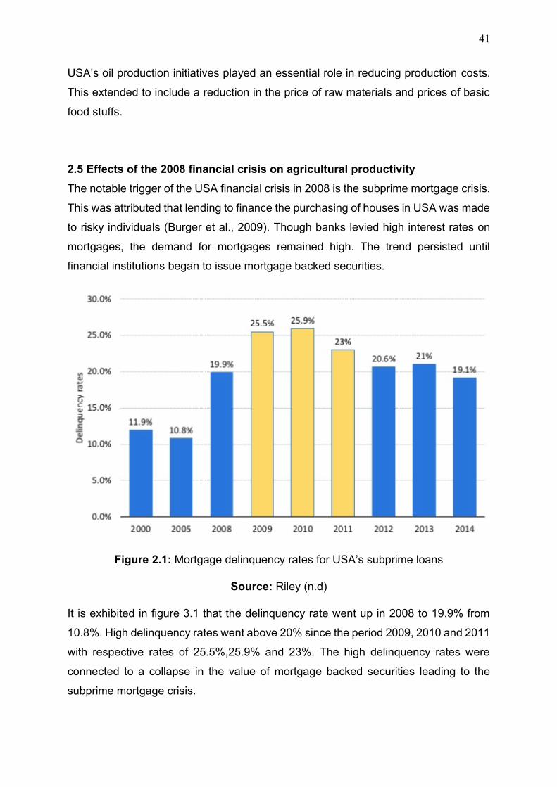
41
USA’s oil production initiatives played an essential role in reducing production costs.
This extended to include a reduction in the price of raw materials and prices of basic
food stuffs.
2.5 Effects of the 2008 financial crisis on agricultural productivity
The notable trigger of the USA financial crisis in 2008 is the subprime mortgage crisis.
This was attributed that lending to finance the purchasing of houses in USA was made
to risky individuals (Burger et al., 2009). Though banks levied high interest rates on
mortgages, the demand for mortgages remained high. The trend persisted until
financial institutions began to issue mortgage backed securities.
Figure 2.1: Mortgage delinquency rates for USA’s subprime loans
Source: Riley (n.d)
It is exhibited in figure 3.1 that the delinquency rate went up in 2008 to 19.9% from
10.8%. High delinquency rates went above 20% since the period 2009, 2010 and 2011
with respective rates of 25.5%,25.9% and 23%. The high delinquency rates were
connected to a collapse in the value of mortgage backed securities leading to the
subprime mortgage crisis.

42
Efforts to examine how the financial crisis affected the USA’s agriculture can be made
possible by examining the related externalities. It can be noted that farmers secured
funding from credit from financial markets but the effect of the mortgage bust imposed
huge negative implications on the ability of farmers to secure funding from financial
markets. Worse when the entire US economy went into a deep recession. Such a
recession did not spare the US agriculture sector. In addition, the performance of the
US’s agriculture sector fell following a decline trade and investment in agricultural
products. This was exacerbated by the imposing of austerity measure by the US
government as the USA’s foreign debt continued to grow severely. Figure 2.2 can also
be used to depict the exist of a nexus linking agricultural productivity, oil prices,
economic growth, financial stability and financial development.
Figure 2.2: Externalities from a financial crisis
Source: Riley (n.d)
43
2.6 Summary
The USA’s economy continues to exhibit strong signs of recovery after experiencing
the ravaging effects of a financial crisis in 2008. With a highly performing economy
that is supported by a well-developed financial system, the USA’s agriculture sector
has managed to thrive well. A lot of agricultural initiatives introduced by the US
government have favourably managed to boost agricultural productivity. This was
supported by oil production initiatives such as the shale oil production strategy which
managed to drive down costs and prices down. however, the 2008 financial crisis
imposed huge negative effects on the entire US economy. Both the financial and
agriculture sectors suffered severely from the effects of the financial crisis. The 2008
USA financial crisis is linked to a lot of economic indicators and this proved the
existence of a nexus linking agricultural productivity, oil prices, economic growth and
financial development.

44
CHAPTER THREE
RESEARCH METHODOLOGY
3.1 Research design
Secondary data from the year 1962 to 2016 was used to estimate an agricultural
productivity model with oil prices, economic growth, financial development and a
financial crisis as regressors. Data estimation was done with the aid of EViews 10 and
the findings were presented in the form of tables and graphs. Model specification tests
were also conducted to determine the reliability, validity and policy usefulness of the
estimated model. Conclusions and policy implications were later deduced from the
computed findings.
3.2 Assumptions
Based on observations and studies concerning the 2008 financial crisis that took place
in the USA, it is highly known that most of the effects were highly evident in 2008
(Brown, 2010; Laux & Leuz, 2010). Though the effects spilt into the first quarter of
2009, it is also highly believed that the financial crisis dissipated in 2008 (Demyanyk
& Van Hemert, 2009; Piskorski, Seru & Vig, 2010; Reinhart & Rogoff, 2008). As a
result, an assumption was made that the financial crisis experienced in the USA
ensued in 2008 and dissipated in the same year. This will have an effect on structural
breaks and hence, Chow Test was applied to test for the existence of a financial break
in the year 2008.
45
3.3 Model estimation techniques
The use of econometric models in academic research is determined by what the study
seeks to accomplish and the extent to which the model variables confine to the given
model stipulations. As a result, an attempt by this study to examine the nexus between
agricultural productivity, oil prices, economic growth and financial development can be
best accomplished by using an Auto Regressive Distributed Lag (ARDL) model. This
is empirically supported by findings made by Pesaran and Shin (1978) which exhibited
that an ARDL model can yield consistent and efficient estimators. Godfrey (1978) also
acknowledges that an ARDL model works the best when variables are integrated of
different orders. That is when the variables have mixed stationarities in which some
variables are I(0) while others are I(I).
At this stage, we can posit that positive changes in agricultural productivity require a
well-functioning economy which is free from the interference of a financial crisis and a
developed financial system. This can mathematically be expressed in a functional form
as follows;
AP = F[OP, EG, FD, FC] ………………………………………………………………… (1).
Where AP denotes changes in agricultural productivity, OP represents variations in oil
prices, EG provides an indication of changes in economic performance as a measured
by gross domestic product (GDP), FD shows the economy’s level of financial
development and the dummy variable FC caters for structural breaks caused by the
prevalence of a financial crisis.
By including a constant α, regression analysis coefficients (β1-βn) and error term (µ)
to equation (1), the resultant expression is a regression model as expressed by
equation (2).
LAP = α + β1LOP + β2LEG + β3LFD + β4DVFC + µ …………………………………… (2).
The ARDL model will thus, be developed based on the model expression depicted by
equation 2. Prior to the estimation of the ARDL model, care is placed on highlighting
that an ARDL model revolves around the determination of short-run and long-model
expressions (Gujarat, 2009). It is thus, in this regard that short-run and long-run model
specifications were determined.

46
Short-run model dynamics
∆LAPt = 𝒂𝟎𝟏 ∑ 𝒂𝟏𝒊𝒑𝒊=𝟏 ∆𝑳𝑨𝑷𝒕−𝟏 + 𝒂𝟐𝒊 ∑ 𝒂𝟑𝒊
𝒑𝒊=𝟏 ∆𝑳𝑶𝑷𝒕−𝟏 + 𝒂𝟒𝒊 ∑ 𝒂𝟓𝒊
𝒑𝒊=𝟏 ∆𝑳𝑬𝑮𝒕−𝟏 +
𝒂𝟔𝒊 ∑ 𝒂𝟕𝒊𝒑𝒊=𝟏 ∆𝑳𝑭𝑫𝒕−𝟏 + 𝒂𝟖𝒊 ∑ 𝒂𝟗𝒊
𝒑𝒊=𝟏 ∆𝑫𝑽𝑭𝑪𝒕−𝟏 +
𝒆𝟏𝒕𝒅(𝑳𝑨𝑷) 𝒄 𝒅(𝑳𝑨𝑷(−𝟏)) 𝒅(𝑳𝑶𝑷(−𝟏))𝒅(𝑳𝑬𝑮(−𝟏)) 𝒅(𝑳𝑭𝑫(−𝟏))𝒅(𝑫𝑽𝑭𝑪(−𝟏)).. (3)
∆LOPt = 𝒂𝟎𝟏 ∑ 𝒂𝟏𝒊𝒑𝒊=𝟏 ∆𝑳𝑶𝑷𝒕−𝟏 + 𝒂𝟐𝒊 ∑ 𝒂𝟑𝒊
𝒑𝒊=𝟏 ∆𝑳𝑨𝑷𝒕−𝟏 + 𝒂𝟒𝒊 ∑ 𝒂𝟓𝒊
𝒑𝒊=𝟏 ∆𝑳𝑬𝑮𝒕−𝟏 +
𝒂𝟔𝒊 ∑ 𝒂𝟕𝒊𝒑𝒊=𝟏 ∆𝑳𝑭𝑫𝒕−𝟏 + 𝒂𝟖𝒊 ∑ 𝒂𝟗𝒊
𝒑𝒊=𝟏 ∆𝑫𝑽𝑭𝑪𝒕−𝟏 +
𝒆𝟏𝒕𝒅(𝑳𝑶𝑷) 𝒄 𝒅(𝑳𝑶𝑷(−𝟏)) 𝒅(𝑳𝑨𝑷(−𝟏)) 𝒅(𝑳𝑬𝑮(−𝟏)) 𝒅(𝑳𝑭𝑫(−𝟏)) 𝒅(𝑫𝑽𝑭𝑪(−𝟏))...
(4)
∆LEGt = 𝒂𝟎𝟏 ∑ 𝒂𝟏𝒊𝒑𝒊=𝟏 ∆𝑳𝑬𝑮𝒕−𝟏 + 𝒂𝟐𝒊 ∑ 𝒂𝟑𝒊
𝒑𝒊=𝟏 ∆𝑳𝑶𝑷𝒕−𝟏 + 𝒂𝟒𝒊 ∑ 𝒂𝟓𝒊
𝒑𝒊=𝟏 ∆𝑳𝑨𝑷𝒕−𝟏 +
𝒂𝟔𝒊 ∑ 𝒂𝟕𝒊𝒑𝒊=𝟏 ∆𝑳𝑭𝑫𝒕−𝟏 + 𝒂𝟖𝒊 ∑ 𝒂𝟗𝒊
𝒑𝒊=𝟏 ∆𝑫𝑽𝑭𝑪𝒕−𝟏 +
𝒆𝟏𝒕(𝑳𝑬𝑮) 𝒄 𝒅(𝑳𝑬𝑮(−𝟏)) 𝒅(𝑳𝑶𝑷(−𝟏)) 𝒅(𝑳𝑨𝑷(−𝟏)) 𝒅(𝑳𝑭𝑫(−𝟏))𝒅(𝑫𝑽𝑭𝑪(−𝟏))... (5)
∆LFDt = 𝒂𝟎𝟏 ∑ 𝒂𝟏𝒊𝒑𝒊=𝟏 ∆𝑳𝑭𝑫𝒕−𝟏 + 𝒂𝟐𝒊 ∑ 𝒂𝟑𝒊
𝒑𝒊=𝟏 ∆𝑳𝑶𝑷𝒕−𝟏 + 𝒂𝟒𝒊 ∑ 𝒂𝟓𝒊
𝒑𝒊=𝟏 ∆𝑳𝑬𝑮𝒕−𝟏 +
𝒂𝟔𝒊 ∑ 𝒂𝟕𝒊𝒑𝒊=𝟏 ∆𝑳𝑨𝑷𝒕−𝟏 + 𝒂𝟖𝒊 ∑ 𝒂𝟗𝒊
𝒑𝒊=𝟏 ∆𝑫𝑽𝑭𝑪𝒕−𝟏 +
𝒆𝟏𝒕𝒅(𝑳𝑭𝑫) 𝒄 𝒅(𝑳𝑭𝑫(−𝟏)) 𝒅(𝑳𝑶𝑷(−𝟏))𝒅(𝑳𝑬𝑮(−𝟏)) 𝒅(𝑳𝑨𝑷(−𝟏)) 𝒅(𝑫𝑽𝑭𝑪(−𝟏))... (6)
∆DVFCt = 𝒂𝟎𝟏 ∑ 𝒂𝟏𝒊𝒑𝒊=𝟏 ∆𝐃𝐕𝐅𝐂𝒕−𝟏 + 𝒂𝟐𝒊 ∑ 𝒂𝟑𝒊
𝒑𝒊=𝟏 ∆𝑳𝑶𝑷𝒕−𝟏 + 𝒂𝟒𝒊 ∑ 𝒂𝟓𝒊
𝒑𝒊=𝟏 ∆𝑳𝑬𝑮𝒕−𝟏 +
𝒂𝟔𝒊 ∑ 𝒂𝟕𝒊𝒑𝒊=𝟏 ∆𝑳𝑭𝑫𝒕−𝟏 + 𝒂𝟖𝒊 ∑ 𝒂𝟗𝒊
𝒑𝒊=𝟏 ∆𝑳𝑨𝑷𝑭𝑪𝒕−𝟏 +
𝒆𝟏𝒕𝒅(𝑫𝑽𝑭𝑪) 𝒄 𝒅(𝑫𝑽𝑭𝑪(−𝟏)) 𝒅(𝑳𝑨𝑷(−𝟏))𝒅(𝑳𝑶𝑷(−𝟏)) 𝒅(𝑳𝑬𝑮(−𝟏)) 𝒅(𝑳𝑭𝑫(−𝟏))..(7)
Using the ARDL model estimation techniques, the long-run ARDL model was therefore
specified as follows;
LAPt = a01 + b11LOP + b22LEG + a33LFD + DVFCt + e1tLAP c LOP(-1) LEG(-1) LFD(-
1) DVFCt(-1) ………………………………………………………………………………..(8)

47
3.4 Model tests
3.4.1 Stationarity tests
The concept of stationarity mainly deals with the need to determine if the variables are
cointegrated of the same order (Dickey & Fuller, 1979). That is, variance and mean of
the data series should not change with time. In a such a case, the data is said to be
stationary and not having a u nit root. For example, a stationary time series, with for
example the case where Yt follows a normal distribution N(mu, sigma^2) independent
of t.
The ability of time series data to yield reliable estimates relies on the extent to which
the variables are stationary. If not, then the results can suffer from a spurious effect
(Madala, 2001). Dickey and Fuller Gujarat (2009) outlined that the estimation of
econometric models requires that certain stationarity conditions be met before
estimation a model. This is specifically true with the estimation of an ARDL model.
Hence, it is always important to test for the presence of a unit root in time series data.
As a result, unit root tests are done either at level or first difference either including a
trend, constant or both trend and constant. This is often accomplished by using
methods such as the Phillips-Perron (PP), Dickey-Fuller (ADF) and KPSS tests.
3.4.2 Granger causality tests
One of the most notable observations that can be made when interpreting econometric
models is that having an effect does not always imply that there is causality among
the variables. As a result, the importance of pairwise Granger causality and exogeneity
block tests is often acknowledged (Toda & Yamamoto, 1995). Granger (1988)
established that causality exists when lagged values of one significantly predict
changes in the other variable. Given residuals E1 and E2, model coefficients grouped
into matrix A, variables X1 and X2 and the number of lags p combined to form
autoregressive models shown by expression (9).
…………………………. (9)

48
We can establish that X2 has causal effects on X1 when the coefficients of matrix A
are jointly significant. In this study, the Pairwise causality test was applied to test the
undermentioned assertions;
• H1: Positive developments in the US financial markets did not cause an
improvement in agricultural productivity.
• H2: An increase in agricultural productivity did not necessitate positive
developments in the US financial markets.
3.4.3 Cointegration tests
The long-run bounds test was used to determine the existence of a long run interaction
between the model variables. The bounds test works under proposition of a null
hypothesis that variables are not cointegrated in the long-run (Pesaran, Shin & Smith,
2001) or simply that there exists no joint significant (Frimpong & Oteng-Abayie, 2006,
p. 7). That is;
• HN: a1 = a2 = a3 = a4 = 0
• HA: a1 ≠ a2 ≠ a3 ≠ a4 ≠ 0
Long run cointegration is established when the computed F-statistic lies beyond both
the lower and upper bounds values leading to the rejection of HN and acceptance of
HA. Computations of the bounds test are based on the inclusion of an error correction
term (ECT), (Engle & Granger, 1987). The importance of an ECT is attached to its
ability to offer insights about the model’s speed of adjustment. Given regressors and
X and R, and a regressand Y, the ECT can be computed as follows;
ECTt-1 = [YT-1 ƞXt-1 – ξRt-1] ……………………………………………………………... (10).
Based on the computed ARDL model that was utilised in this study, the error correction
model can thus be specified as follows;
∆LAPt = 𝒂𝟎 ∑ 𝒂𝟏𝒊𝒑𝒊=𝟏 ∆𝑳𝑨𝑷𝒕−𝟏 + 𝒂𝟐𝒊 ∑ 𝒂𝟑𝒊
𝒑𝒊=𝟏 ∆𝑳𝑶𝑷𝒕−𝟏 + 𝒂𝟒𝒊 ∑ 𝒂𝟓𝒊
𝒑𝒊=𝟏 ∆𝑳𝑬𝑮𝒕−𝟏 +
𝒂𝟔𝒊 ∑ 𝒂𝟕𝒊𝒑𝒊=𝟏 ∆𝑳𝑭𝑫𝒕−𝟏 + 𝒂𝟖𝒊 ∑ 𝒂𝟗𝒊
𝒑𝒊=𝟏 ∆𝑫𝑽𝑭𝑪𝒕−𝟏 +
𝒆𝟏𝒕 𝒅(𝑳𝑨𝑷) 𝒄 𝒅(𝑳𝑨𝑷(−𝟏)) 𝒅(𝑳𝑶𝑷(−𝟏))𝒅(𝑳𝑬𝑮(−𝟏)) 𝒅(𝑫𝑽𝑭𝑪(−𝟏)) ECT(-1)
49
3.4.4 Sensitivity analysis
In econometrics, it is important to carry out diagnostic tests on any estimated model
so as to ensure that the model is capable of offering reliable results that can be used
for policy making (Greene, 2003). That is, to check to see if the model is not
misspecified and can accurately predict or estimate the actual and intended effects.
Notable diagnostics tests that were carried in this study are;
• Heteroscedasticity tests: In some cases, the variance of the error terms might
be heteroscedastic and in such a case, the model is considered to be suffering
from heteroscedasticity problems (Greene, 2003). Heteroscedasticity poses
huge negative implications on the estimated model. For instance, Greenberg
and Webster (1983) concurs with this notion and contend that
heteroscedasticity causes the standard errors to be biased. Craven and Islam
(2011) also concur with this idea and posit that the problem of also extends to
affect the statistical significance of the model parameters. That is,
heteroscedasticity can cause significant coefficients to appear as insignificant.
It is in this regard that the agricultural productivity nexus model was subjected
to the Arch and Breusch-Godfrey-Pagan heteroscedasticity tests. The effort
was to test if the undermentioned statements hold.
• H0: The agricultural productivity nexus model does not suffer from
the problem of heteroscedasticity.
• H1: The agricultural productivity nexus model suffers from the
problem of heteroscedasticity.
• Serial correlation: Serial correlation occurs when the error terms are
negatively correlated or positively correlated with each other (Gujarat, 2003). It
is of paramount importance to note that serial correlation undermines the
reliability of the estimated model. This is irrespective of the nature of serial
correlation being observed. Hence, attention in this study was devoted towards
determining if the agricultural productivity nexus model succumbs to serial
correlation. The Breusch-Pagan-Serial Correlation LM test was used to test for
serial correlation at 0.05% in line with the following hypothesis;
• H0: The agricultural productivity nexus model does not suffer from
the problem of serial correlation.

50
• H1: The agricultural productivity nexus model suffers from the
problem of serial correlation.
• Normality test: Normality tests whether the distribution of the model variables
is normal over the course of the period under study. It is important for an
estimated model to conform to normality diagnostic tests if its reliability and
validity are to be considered as up to standard (Greene, 2003). The Jarque-
Bera test statistic was used to indicate whether the variables are normally
distributed over the period 1962-2016 by testing the following hypothesis at 5%
significance level.
• H0: LAP, LOP, LFD, LEG and FC are normally distributed over the period
1962-2016.
• H1: LAP, LOP, LFD, LEG and FC are not normally distributed over the
period 1962-2016.
• Redundancy tests: One of the core features of a good estimated model is that
it must not be redundant. That is, the variables must be jointly significant
(Gujarat, 2009). This is determined in line with the hypotheses that the variables
are jointly insignificant. In this case, the redundancy test will be based on the
need to determine if the following hypothesis will hold at 5%;
• H0: LOP, LFD, LEG and FC are jointly insignificant.
• H1: LOP, LFD, LEG and FC are jointly significant.
• Stability tests: Stability tests provides an indication of how stable the
estimated model is over the period under study. This is important because any
model that is not stable will be incapable to offer any useful policy-making
suggestions (Ploberger & Krämer, 1990). It is in this regard that attention was
placed towards determining the stability of the agricultural productivity nexus
model. The stability of the agricultural productivity nexus model was determined
using Cusum and Cusum of squares tests. Cusum and Cusum of squares tests
posit that a model is stable when the Cusum lies within the 5% significance limit
(Hansen, 1992).

51
3.5 Definition of variables and the expected impact
Table 4.1 provides a description of the variables that will be used in this study including
their expected relationships with the independent variable economic growth.
Table 3.1: Definition of variables and expected impact
Variable Definition Expected
Impact
Dependent
Variable
Agriculture
output
(AO)
Refers to the total agricultural output that is produced
by the agriculture sector of an economy over a given
period of time. The more productive an economy is
the more agricultural output is produced by the
agriculture sector. Agricultural imports will be used a
proxy for agricultural productivity. The idea is that the
more productivity the economy will be, the less
agricultural products will be imported.
Independent
variables
Oil prices
(OP)
Provides a measure of changes in crude oil prices as
of the period under study (1962 to 2016).
(-)
Economic
growth
(EG)
Provides a measure of economic performance and
will be measured using gross domestic product
(GDP).
(+)
Financial
development
(FD)
Is simply a reflection of financial sophistication and
deepening of an economy’s financial sector and its
ability to reduce financial costs.
(+)
Financial
crisis
(FC)
The economic crisis is represented by a dummy
variable which either takes a value of 0 to
characterise a period in which there were no
incidences of an economic crisis and 1 period which
an economy was considered to be suffering from an
economic crisis.
(-)
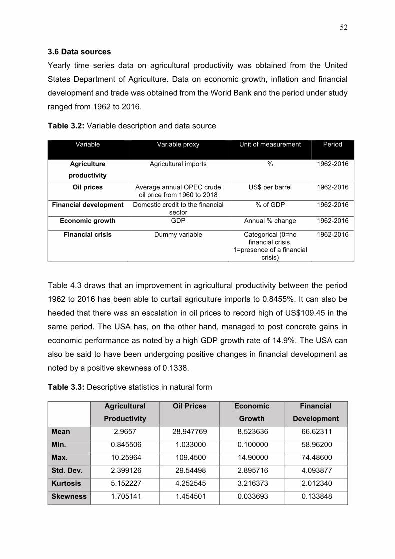
52
3.6 Data sources
Yearly time series data on agricultural productivity was obtained from the United
States Department of Agriculture. Data on economic growth, inflation and financial
development and trade was obtained from the World Bank and the period under study
ranged from 1962 to 2016.
Table 3.2: Variable description and data source
Variable Variable proxy Unit of measurement Period
Agriculture
productivity
Agricultural imports % 1962-2016
Oil prices Average annual OPEC crude oil price from 1960 to 2018
US$ per barrel 1962-2016
Financial development Domestic credit to the financial sector
% of GDP 1962-2016
Economic growth GDP Annual % change 1962-2016
Financial crisis Dummy variable Categorical (0=no financial crisis,
1=presence of a financial crisis)
1962-2016
Table 4.3 draws that an improvement in agricultural productivity between the period
1962 to 2016 has been able to curtail agriculture imports to 0.8455%. It can also be
heeded that there was an escalation in oil prices to record high of US$109.45 in the
same period. The USA has, on the other hand, managed to post concrete gains in
economic performance as noted by a high GDP growth rate of 14.9%. The USA can
also be said to have been undergoing positive changes in financial development as
noted by a positive skewness of 0.1338.
Table 3.3: Descriptive statistics in natural form
Agricultural
Productivity
Oil Prices Economic
Growth
Financial
Development
Mean 2.9657 28.947769 8.523636 66.62311
Min. 0.845506 1.033000 0.100000 58.96200
Max. 10.25964 109.4500 14.90000 74.48600
Std. Dev. 2.399126 29.54498 2.895716 4.093877
Kurtosis 5.152227 4.252545 3.216373 2.012340
Skewness 1.705141 1.454501 0.033693 0.133848

53
Oil prices, economic growth and financial development have high elastic responses
as noted by their respective mean values of 2.701, 2.033 and 4.197. Much of the
variation that was observed between the period 1962 to 2016 is mainly attributed to
changes in oil prices which had a high standard deviation of 1.379.
Table 3.4: Descriptive statistics in log form
Agricultural
Productivity
Oil Prices Economic
Growth
Financial
Development
Mean 0.827098 2.701029 2.033206 4.197201
Min. -0.167820 0.032467 -2.302585 4.076893
Max. 2.328218 4.695468 2.701361 4.310611
Std. Dev. 0.688733 1.379107 0.672046 0.061379
Kurtosis 2.481189 2.390054 32.80784 2.023687
Skewness 0.527485 -0.665877 -4.956793 0.041754
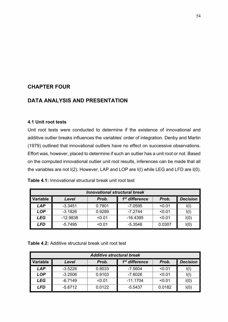
54
CHAPTER FOUR
DATA ANALYSIS AND PRESENTATION
4.1 Unit root tests
Unit root tests were conducted to determine if the existence of innovational and
additive outlier breaks influences the variables’ order of integration. Denby and Martin
(1979) outlined that innovational outliers have no effect on successive observations.
Effort was, however, placed to determine if such an outlier has a unit root or not. Based
on the computed innovational outlier unit root results, inferences can be made that all
the variables are not I(2). However, LAP and LOP are I(I) while LEG and LFD are I(0).
Table 4.1: Innovational structural break unit root test
Innovational structural break
Variable Level Prob. 1st difference Prob. Decision
LAP -3.3451 0.7801 -7.0595 <0.01 I(I)
LOP -3.1826 0.9289 -7.2744 <0.01 I(I)
LEG -12.9838 <0.01 -16.4395 <0.01 I(0)
LFD -5.7495 <0.01 -5.3546 0.0307 I(0)
Table 4.2: Additive structural break unit root test
Additive structural break
Variable Level Prob. 1st difference Prob. Decision
LAP -3.5226 0.8033 -7.5604 <0.01 I(I)
LOP -3.2506 0.9103 -7.6026 <0.01 I(I)
LEG -6.7149 <0.01 -11.1704 <0.01 I(0)
LFD -5.6712 0.0122 -5.5437 0.0182 I(0)
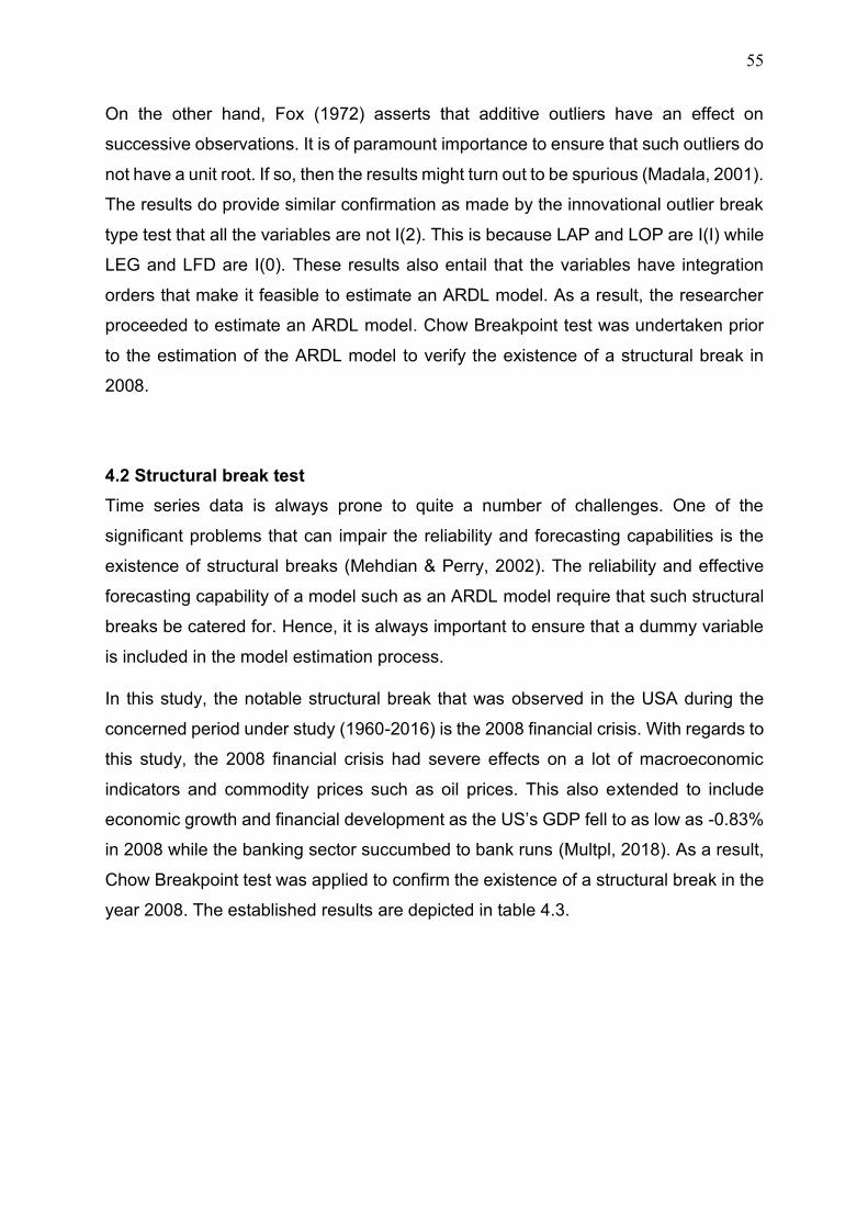
55
On the other hand, Fox (1972) asserts that additive outliers have an effect on
successive observations. It is of paramount importance to ensure that such outliers do
not have a unit root. If so, then the results might turn out to be spurious (Madala, 2001).
The results do provide similar confirmation as made by the innovational outlier break
type test that all the variables are not I(2). This is because LAP and LOP are I(I) while
LEG and LFD are I(0). These results also entail that the variables have integration
orders that make it feasible to estimate an ARDL model. As a result, the researcher
proceeded to estimate an ARDL model. Chow Breakpoint test was undertaken prior
to the estimation of the ARDL model to verify the existence of a structural break in
2008.
4.2 Structural break test
Time series data is always prone to quite a number of challenges. One of the
significant problems that can impair the reliability and forecasting capabilities is the
existence of structural breaks (Mehdian & Perry, 2002). The reliability and effective
forecasting capability of a model such as an ARDL model require that such structural
breaks be catered for. Hence, it is always important to ensure that a dummy variable
is included in the model estimation process.
In this study, the notable structural break that was observed in the USA during the
concerned period under study (1960-2016) is the 2008 financial crisis. With regards to
this study, the 2008 financial crisis had severe effects on a lot of macroeconomic
indicators and commodity prices such as oil prices. This also extended to include
economic growth and financial development as the US’s GDP fell to as low as -0.83%
in 2008 while the banking sector succumbed to bank runs (Multpl, 2018). As a result,
Chow Breakpoint test was applied to confirm the existence of a structural break in the
year 2008. The established results are depicted in table 4.3.
56
Table 4.3: Chow Breakpoint test
Chow Breakpoint
F-stat. 3.6691 Prob. F(5,45) 0.0072
Log L.R. 18.8067 Prob. Chi-square (5) 0.0021
Wald stat. 18.3454 Prob. Chi-square (5) 0.00235
HO: No break in the year 2008
Using the depicted breakpoint test results, it can, therefore, be affirmed that there was
a structural break in 2008. This, therefore, reinforces the influence of the 2008 financial
crisis on agricultural productivity, oil prices, financial development and economic
growth. Hence, a dummy variable (DVFC) was incorporated into the model estimation
so as to capture the prevalence of the financial crisis.
4.3 Correlation coefficient test
Pearson correlation test was employed so as to establish the strength of the
association between the variables. The results depict that oil prices and agricultural
productivity are negatively and significantly correlated by 0.9227. This implies that
upwards changes in oil prices are more likely to be associated with a decline in
agricultural productivity. The results also depict that there is a relatively moderate
positive correlation between economic growth and agricultural productivity of 0.4572.
Which denotes that the US economy benefits relatively more from increases in
agricultural productivity as more agricultural output is exported and less is imported.
Deductions can also be made that both agricultural productivity and economic growth
are negatively and insignificantly correlated with a financial crisis by 0.1358 and
0.2501 respectively. This can be utilized as proof that not only the financial sector
suffers from the effects of the financial crisis but also other sectors such as the
agriculture sector. The economy at large also suffers from the ravaging adverse effects
of a financial crisis. Implications can be made that agricultural productivity and financial
development are negatively correlated. This is because a significant correlation of -
0.4362 exists between agricultural productivity and financial development. Possible
reasons can be pointed towards people switching to other assets and investments in
other sectors of the economy.

57
Table 4.4: Pearson correlation coefficient test
Financial development is positively and insignificantly correlated with a financial crisis
by 0.0777. This is possible because, in the short run, firms in the financial sectors will
be taking advantage of the windfall gains experienced from the effects of the financial
crisis. The significant negative correlation between economic growth and financial
development of 0.2835 entails that developments in the financial sector are hampering
economic growth and development. This can be supported by insights provided by
Caporale et al. (2009) which pointed out that issues like high lending rates can reverse
the positive gains of financial development. Caporale and others went on to establish
that financial development can actually hinder economic growth especially when the
quality of borrowers is poor. De Gregorio and Guidotti (1995) established that a
negative correlation can exist especially the financial sector is liberalised in a poor
regulatory environment.
4.4 ARDL Bounds test
The study adopted the bounds test with an emphasis on striving to establish if
agricultural productivity, oil prices, economic growth, financial development are
cointegrated in the long run. Since the obtained significant F-statistic lies above both
the lower and upper bounds values, conclusions can be inferred that the model
LAP LOP LEG LFD FC
LAP ρ 1
P-Value
LOP ρ 92270. - 1
P-Value 00000.
LEG ρ 45720. 33240. - 1
P-Value 00.000 21300.
LFD ρ 26430. - 48310. 8350.2 - 1
P-Value 90.000 00020. 0360.0
FC ρ -0.1358 0.1194 -0.2501 0.0777 1
P-Value 0.3227 0.3854 0.0654 0.5726

58
variables are cointegrated in the long run. In addition, it can be established that
77.21% of the observed variations in agricultural productivity are explained by LOP,
LFD, LEG and FC.
Table 4.5: ARDL Cointegration Test
Significance level
1% 2.5% 5% 10%
F-Statistic LB UB LB UB LB LB LB UB DW
9.488540
k=4
3.29 4.37 2.88 3.87 2.56 3.49 2.20 3.09 2.24
R2 = 0.7721 Adj. R2 = 0.6440 Prob. F stat. = 0.00000
4.4.1 Cointegrating form
The cointegration term is negative and significant at 1% signifying the existence of
cointegration in the short run between AP, OP, EG, FD, and FC. Also, the cointegration
value of 0.1519 implies that the speed of adjustment is 15.19%. Thus, the previous
years’ deviations from long-run equilibrium are corrected in the same year at a speed
of 15.19%. Alternatively, it can posit that AP, OP, FD, EG and FC will revert back to
their equilibrium position in the same year at a speed of 15.19%.
Table 4.6: Cointegrating form
Variable Coefficient Std. Error t-statistic Prob.
Coint EqT (-1) -0.151900 0.018722 -8.113368 0.0000*
Cointeq = LAM – (0.2042*LOP + 2.2714*LFD + 0.4788*LEG – 0.6413 – 9.4633)
4.4.2 Short run bounds test results
The depicted results denote that previous levels of agricultural productivity influence
proceeding levels of agricultural productivity. This is because agricultural productivity
remained in an unfavourable state at both lag 1, 2 and 3 with respective values of -
0.1222, -0.3079 and -0.2934.

59
The results also show that there were series of short run volatile changes in oil prices
between the period 1962 to 2016. This can be evidenced by decline in oil prices from
a positive effect of 0.0051 to a negative effect of 0.011877 in the first lag. The effect
later increased from a negative effect of -0.11877 to a positive effect 0.069462 in the
second lag.
In the short run, GDP can be observed to have been significantly falling at both the
first lag and second lag suggesting a decline in economic performance. This can
trigger negative effects in other sectors through contagion effects and this can in turn
affect agricultural productivity.
Table 4.7: Short run bounds test estimations
Variable Coefficient Std. Error t-statistic Prob.
D(LAM(-1)) -0.1222204 0.106556 -1.146858 0.2599
D(LAM(-2)) -0.307906 0.086590 -3.555917 0.0012
D(LAM(-3)) -0.293390 0.075093 -3.906994 0.0005
D(LOP) 0.001573 0.020199 0.077880 0.9384
D(LOP(-1)) -0.011877 0.022889 -0.518905 0.6074
D(LOP(-2)) 0.069462 0.023075 3.010206 0.0051
D(LEG) 0.027848 0.009197 3.027853 0.0048
D(LEG(-1)) -0.025061 0.013575 -1.846104. 0.0741
D(LEG(-2)) -0.046414 0.011483 -4.042071 0.0003
D(LFD) -1.246021 0.267465 -4.658632 0.0001
D(LFD(-1)) 0.628604 0.381918 1.645913 0.1096
D(LFD(-2)) -1.322145 0.344690 -3.835753 0.0006
D(LFD(-3)) 0.469393 0.269363 -1.762608 0.0910
C -1.437466 0.622676 -2.308528 0.0276
R2 = 0.882493 Adj. R2 = 0.814180
Prob. F stat. 0.00000 DW. Stat. = 2.254427
Periods of instabilities can also be observed to have existed in the USA’s financial
sector. This is because the extent to which financial development contributes towards
improving agricultural productivity went up from -1.246021 to 0.628604 in the first lag.
Also, the capacity of financial development to increase and contribute positively

60
towards agricultural productivity went down in the second lag. The effective capacity
of financial went down from 0.628604 to -1.322145 in the second lag but later went up
to 0.469393 in the third lag. 88.25% of the short run changes in agricultural productivity
are attributed to changes in oil prices, economic growth, prevalence of a financial crisis
and financial development.
4.4.3 Long run bounds test
After having confirmed the existence of a long run association between agricultural
productivity, oil prices, financial development and economic growth, the researcher
proceeded to interpret the established long run results.
The results do show that financial development and agricultural productivity are
unilaterally linked by 2.271356. This entails that an improvement in financial
development by 1% will initiate positive variations in agricultural productivity by
227.14%. Rizwan-ul-Hassan (2017) concurs with this result and asserts that this is as
a result of the ability of the financial sector to finance the acquisition of high-payoff
agricultural technology.
Table 4.8: Long run bounds test
Variable Coefficient Std. Error t-statistic Prob.
Financial Development 2.271356 1.046655 2.170110 0.0375**
Economic Growth 0.478784 0.121171 3.951310 0.0004*
Oil Prices -0.204163 0.069567 -2.934763 0.0061*
Financial Crisis -0.641288 0.183113 -3.502145 0.0014*
C -9.463268 4.388919 -2.156173 0.0387**
* and ** = p < 0.01 and p < 0.05 respectively
R2 = 0.772143 Adj. R2 = 0.643973 Prob. F stat. 0.00000 DW. Stat. = 2.241140
The results also establish similar deductions as those made by Amone (2014), and
Ismail and Kabuga (2016) who highlighted that economic growth favours agricultural
productivity can also be made in this study. This is because an increase in economic
growth by 1% agitates an increase in agricultural productivity by 47.88%. This is

61
possibly attributed to the enactment of growth strategies, agricultural policies and
institutional stability measures which favour agricultural productivity.
Theoretical ideas ascertained from the high payoff input model postulate that the
degree to which financial development contributes towards promoting agricultural
productivity is determined by financial stability. The obtained results reinforce this
assertion and denote that a surge in oil prices by US1 will result in a decline in
agricultural productivity by 20.41%. Wang and McPhail (2014) also acknowledged this
and hinted that it is a huge challenge for the agriculture sector to thrive when oil prices
are surging up high.
The results also support ideas deduced from the high payoff input model which
suggests that economic disturbances such as a financial crisis can hinder agricultural
productivity. This can be heeded to be true since an increase in the financial crisis by
1% results in a decline in agricultural productivity by 64.63%. Deepak (2012) also
accepted this idea and outlined that farmers usually fail to access the required capital
funding during periods of a financial crisis. As a such, agricultural productivity tends to
decline during a period characterised by incidences of a financial crisis.
It can further be deduced that 77.21% of the variation in agricultural productivity is
attributed to changes in agricultural productivity, oil prices, economic growth, financial
crisis and financial development. Thus, 22.79% of the changes in agricultural
productivity, are attributed to changes in other variables outside the estimated model.
4.5 Sensitivity analysis
Ramsey Reset test by Ramsey and Schmidt (1976), was employed so as to determine
whether the variables have an element of non-linearity or not. In light of the reported
Ramsey Reset test findings, conclusions can be made that the ARDL model has no
non-linearity features. That is, the model is linear and this is because the null
hypothesis of linearity is accepted at 5% (χ2=0.3880; ρ=0.5379).

62
Table 4.9: Sensitivity analysis
𝜒2𝑅𝑅 𝜒2N 𝜒2𝐴𝑅 𝜒2𝐵𝑅 𝜒2𝑆𝐶
0.3880
(0.5379)
0.0607
(0.9701)
0.0495
(0.8204)
0.5112
(0.9991)
1.6725
(0.0775)
NOTE: RR, N2
, BR2
, AR2
and SC2
Ramsey Reset Test, langrage multiplier for normality, Arch test for heteroscedasticity at lag 1, Breusch-Godfrey-Pagan test for heteroscedasticity and serial correlation at 2 lags. The values in parenthesis are the corresponding P-Value.
Sensitivity analysis was also undertaken with respect to normality, heteroscedasticity
(arch, Breusch-Pagan-Godfrey) and serial correlation tests. Respective p-values of
0.9701, 0.8204, 0.9991 and 0.0775 were recorded and this purports that the variables
are normally distributed and that heteroscedasticity and serial correlation problems
are not evident. As a result, it can thus be concluded that that the estimated model
does meet the necessary sensitivity standards and can be safely used for
policymaking.
4.6 Redundant variable test
An attempt was made to determine if OP, FD, EG and FC are jointly significant in
explaining possible variations in agricultural productivity. That is, to ascertain whether
the inclusion of the variables will enhance the statistical significance of the explanatory
power of the exogenous variables. This was accomplished by using the redundant
variable test and works to tests the validity of the following statements;
• H0: LOP, LFD, LEG and FC are jointly insignificant.
• H1: LOP, LFD, LEG and FC are jointly significant.
Table 4.10: Redundant variable test
Redundant test on LOP, LFD, LEG and DVFC
Value Df Prob.
F-statistic 14.33562 (4, 32) 0.0000

63
Having an F-statistic of 14.336 with an associated p-value of 0.0000 implies that H0
can be rejected at 5% (ρ<0.05) and conclude that the variables are jointly significant.
The results thus, provide strong evidence that OP, FD, EG and FC are jointly
significant in explaining possible variations in agricultural productivity in the USA.
4.7 Stability tests
Cusum and Cusum of squares stability inquiries were employed so as to ascertain if
the formulated model can be declared to be stable over the course of the study which
has been established to be 1960 to 2016. Based on figure 5.1 presentation, it can be
heeded that the model confines within the critical bounds. Hence, inferences can be
established that the formulated ARDL model is stable over the period 1960-2016.
Figure 4.1: Cusum stability inquiries
Source: Developed by Author based on the formulated model
4.8 Model performance and forecast error diagnosis
Model performance and forecast error diagnosis were also undertaken to determine
whether the predictive power of the computed ARDL model is satisfactory and free
from biases. This was accomplished using a dynamic forecasting technique. The
reason behind the use of a dynamic forecasting model is justified by the fact that it
accounts for time-dependent changes or events (Evensen, 1994). This is of paramount
importance, especially when considering the effect of structural breaks and seasonal
changes that impose effects on economic variables.
-20
-15
-10
-5
0
5
10
15
20
86 88 90 92 94 96 98 00 02 04 06 08 10 12 14 16
CUSUM 5% Significance
-0.4
-0.2
0.0
0.2
0.4
0.6
0.8
1.0
1.2
1.4
86 88 90 92 94 96 98 00 02 04 06 08 10 12 14 16
CUSUM of Squares 5% Significance
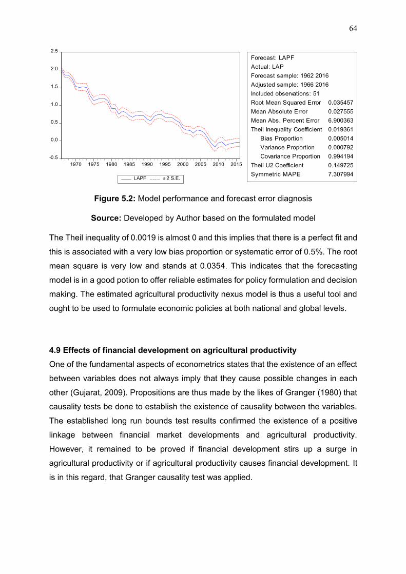
64
-0.5
0.0
0.5
1.0
1.5
2.0
2.5
1970 1975 1980 1985 1990 1995 2000 2005 2010 2015
LAPF ± 2 S.E.
Forecast: LAPF
Actual: LAP
Forecast sample: 1962 2016
Adjusted sample: 1966 2016
Included observations: 51
Root Mean Squared Error 0.035457
Mean Absolute Error 0.027555
Mean Abs. Percent Error 6.900363
Theil Inequality Coefficient 0.019361
Bias Proportion 0.005014
Variance Proportion 0.000792
Covariance Proportion 0.994194
Theil U2 Coefficient 0.149725
Symmetric MAPE 7.307994
Figure 5.2: Model performance and forecast error diagnosis
Source: Developed by Author based on the formulated model
The Theil inequality of 0.0019 is almost 0 and this implies that there is a perfect fit and
this is associated with a very low bias proportion or systematic error of 0.5%. The root
mean square is very low and stands at 0.0354. This indicates that the forecasting
model is in a good potion to offer reliable estimates for policy formulation and decision
making. The estimated agricultural productivity nexus model is thus a useful tool and
ought to be used to formulate economic policies at both national and global levels.
4.9 Effects of financial development on agricultural productivity
One of the fundamental aspects of econometrics states that the existence of an effect
between variables does not always imply that they cause possible changes in each
other (Gujarat, 2009). Propositions are thus made by the likes of Granger (1980) that
causality tests be done to establish the existence of causality between the variables.
The established long run bounds test results confirmed the existence of a positive
linkage between financial market developments and agricultural productivity.
However, it remained to be proved if financial development stirs up a surge in
agricultural productivity or if agricultural productivity causes financial development. It
is in this regard, that Granger causality test was applied.

65
Table 4.11: Pairwise Granger causality test
AP OP FD EG FC
χ2 prob. χ2 prob. χ2 prob. χ2 prob. χ2 prob.
AP - - 2.5605 0.0878 0.5926 0.5569 4.6894 0.0138 0.1581 0.8542
OP 6.2445 0.0039 - - 1.2699 0.2901 2.8640 0.0668 5.5006 0.0071
FD 0.4932 0.6137 0.3625 0.6978 - - 3.0530 0.0565 0.0289 0.9715
EG 2.0377 0.1414 0.3241 0.7247 7.1215 0.0020 - - 1.8611 0.1665
FC 4.8648 0.0119 0.3743 0.6898 0.56144 0.5726 1.2391 0.2987 - -
The results indicate that during the period 1960 to 2016, financial development did not
Granger cause an increase in agricultural productivity. Alternatively, agricultural
productivity did not also granger cause financial development during the same period
of time.
Table 4.12: Summary of the hypothesis tests
Null hypothesis (H0) Test
method
p Decision
Positive developments in US financial markets did not
cause an improvement in agricultural productivity.
Granger
causality
0.6978 Accept
An increase in agricultural productivity did not necessitate
positive developments in the US financial markets
Granger
causality
0.2901 Reject
As a result, it can thus be rejected that positive developments in the US financial
markets did not cause an improvement in agricultural productivity. Similarly, an
increase in agricultural productivity did not necessitate positive developments in US
financial markets.
4.10 Discussion of findings and answers to the research questions
Foremost, it can be established that agricultural productivity is vital at both national
and global levels. This is because it helps in alleviating poverty and attaining MDGs.
In addition, the importance of agricultural productivity mainly lies in its potency to stir
economic growth and development. Furthermore, an increase in agricultural
66
productivity helps to ease pressure on international organisations such as the WFP to
provide food relief programs to poor countries. The notable difference between poor
and rich countries have been noted to be as a result of the inability of poor countries
to possess high-payoff technology. This can possibly explain why the USA is
dominating other countries in terms of economic growth and development. It is
imperative to note that the importance of agricultural growth also extends to
incorporate aspects such as nutrition, food security, subsistence income and raising
domestic employment levels. However, positive changes in the agriculture sector are
highly dependent on the interaction between the availability of financial support,
economic stability and performance. As a result, changes in the prices of factor inputs,
the ability to secure funding from financial institutions to acquire high-payoff
technology, economic stability and performance are thus linked to developments
occurring in the agriculture sector. Alternatively, it can be said that there is a nexus
which links together agricultural productivity, oil prices, economic growth and financial
development. This is highly evident in the USA which is characterised by high growth
rates, has a well-developed financial system and suffered severely from the oil crisis
and the prevalence of the 2008 financial crisis. The study thus, emphasises the
importance of maintaining stability in financial and commodity markets, and the
economy at large. More so, it highlights that economic growth strategies targeted at
improving agricultural productivity through the effective and efficient use of resources
have positive implications for financial development. It must, however, be noted that
investments in the agriculture sector are determined by the effective and efficient use
of resources by the agriculture sector. However, this relies on financial, commodity
markets and economic stability. Such an interaction, therefore, illustrates the existence
of a nexus between agriculture growth, economic and financial stability, and
macroeconomic variables.
67
Determination of the existence of an interaction between agricultural
productivity, oil prices, economic growth and financial development and how oil
prices, economic growth and financial development influence agricultural
productivity.
The computed results through the use of the Bounds test have proved the existence
of a nexus linking agricultural productivity, oil prices, economic growth and financial
development in both the short run and long run. This relates to the ability of farmers to
secure funding for the acquisition of the high payoff input technology, deal with high
oil prices and the effects of a financial crisis, and benefit from economic growth
projects and strategies.
It is also imperative that supply of funds by the financial sector aids farmers in securing
the high payoff input technology which enhances agricultural productivity. As a result,
farmers will be capable of producing more agricultural produce at a relatively low cost.
Consequently, mass production of agricultural produce will cut down agricultural
imports and boost agricultural export levels. The decline in agricultural imports and an
increase in agricultural exports results in an increase in economic growth through an
improvement in the current account balance. Also, this will have multiplier effects on
financial development because rising agriculture income allows farmers to repay back
their bank loans and secure more funds from banks. Along similar lines, there will be
a reduction in non-performing loans and an increase in service fees levied on bank
loans. A case in point is that this will stimulate financial innovation as banks will
endeavour to provide better and affordable financial services to the financial sector. A
significant number of studies did not address this ripple and two-way effect between
agricultural productivity, economic growth and financial development. However, the
high payoff input model does emphasise the importance of providing funds to the
agriculture sector. This therefore, implies that efforts to promote agriculture
productivity are not solely determined by microeconomic variables but also
macroeconomic aspects at large.

68
The ability of the US’s agriculture sector to thrive and maintain high productivity
levels
The positive relationship that exists between agricultural productivity and economic
growth significantly proves that the US’s agriculture sector can thrive and maintain
high productivity levels. This is similar to what has been established from the high
payoff input model which asserts that economic growth policies will target to ensure
that there is increased investment in agriculture. Such a notion has been established
to be true by a significant number of studies which strongly argue that economic growth
and development policies inevitably work towards improving agricultural productivity.
This is because economic policies such as unemployment, foreign direct investment,
poverty reduction, food security etc., will inevitably incorporate agricultural
productivity.
How oil shocks and volatile changes in oil prices affect agricultural productivity.
The impact of economic growth on agricultural productivity can however, be
undermined by rising or volatile oil prices. This is because oil is a major source of
energy in the agriculture sector and rising oil prices will therefore, undermine
productive capacity and cost minimization efforts. Hence, such an observation strongly
provides evidence that rising oil prices have an adverse effect on agricultural
productivity. Quite a number of studies agree with this notion and establish that
reducing factor input costs is pivotal in improving agricultural productivity. Hence, it
remains important for policymakers to develop measures that curb the effect of rising
oil prices.
The extent to which US financial sector developments have stimulated
agricultural productivity and the capacity of agricultural productivity to stir up
financial development in the USA.
The proposed hypothesis was rejected and conclusions were made that positive
developments in the US financial markets did not cause an improvement in agricultural
productivity. This is possible because the US financial market had gone through a
rough period during the period 1962 to 2016. This is because the US economy

69
succumbs to severe effects of the 2008 financial crisis which impaired the effective
distribution or allocation of funds to productive economic sectors. Thus, the US’s
agriculture suffered a lot during and after the occurrence of the 2008 financial crisis.
Moreover, the allocation of funds was relatively biased towards real estate more as
evidenced by the subprime mortgage crisis. This entails that there was a decline in the
potency of farmers to fund the acquisition of high-payoff technology. As a result,
economic growth plummeted as the financial sector went into a doldrum.
It was however noted that an increase in agricultural productivity resulted in positive
developments in the US financial markets. This is because the agriculture sector was
relatively unaffected but disturbances in the USA financial market. Also, financial
players turned to other sectors such as the agriculture sector following the turbulence
experienced in the real estate sector. As a result, the agriculture sector started
experiencing notable improvements which resulted in financial innovation. It is in this
regard that an increase in agricultural productivity resulted in positive developments in
the US financial markets. This is the gap which most empirical studies do not address.

70
CHAPTER FIVE
CONCLUSIONS, POLICY IMPLICATIONS AND SUGGESTIONS FOR
FUTURE RESEARCH
5.1 Conclusions
The study examines the existence of a nexus linking agricultural productivity, oil prices,
economic growth and financial development. The study is motivated by observations
made that efforts to promote agricultural productivity are not solely determined by
microeconomic variables alone. The study thus argues that macroeconomic variables
such as economic growth and financial development and economic events such as oil
shocks and financial crises have an important bearing on agricultural productivity. The
study thus, concluded that there are short run and long run interactions linking
agricultural productivity, oil prices, economic growth and financial development. Such
an interaction works towards improving agricultural productivity but can be impaired
by oil shocks and financial crises.
Though significant number of researches on the determinants of agricultural
productivity are highly focused on the influence of microeconomic determinants,
macroeconomic determinants also posed a huge effect on agricultural productivity.
The effectiveness of microeconomic determinants is largely influenced by the
A combination of oil shocks and a financial crisis poses huge adverse effects on the
interaction linking agricultural productivity, oil prices, economic growth and financial
71
development. It can be noted that oil is one of the major sources of energy used in the
agriculture sector. Hence, disruptions in oil supply caused by rising oil prices are more
likely to undermine productivity initiatives. More so, oil shocks have contagion effects
on other economic sectors which either directly or indirectly connected to agriculture.
For instance, an increase in oil prices will instantly stir an increase in transport fares.
As a result, the cost of transporting agricultural inputs and products will rise in
response to the price increases. The effects of price increases can be eased by a
similar response on agricultural produce. However, this will in turn, result in inflation
and the effects of inflation will be transmitted to other economic sectors. Ultimately, a
nexus will be established between oil prices and other macroeconomic variables. This
strongly reveals that there is a nexus that links macroeconomic variables.
The financial sector remains a key player in efforts to promote agricultural productivity
and the ability of farmers to boost productivity hinges on the performance of the
financial sector. Any economic misfortunes are thus more likely to disturb the
acquisition of high input technology and this will negatively undermine agricultural
productivity. This is highly notable when the economy is going through a financial
crisis. A financial crisis can disrupt the provision of financial service to farmers and
agriculture-related activities. Consequently, the performance of the agriculture sector.
This can be reinforced by observations made in the USA which exhibited that the
allocation of funds was more biased towards real estate. The agriculture was
adversely affected. In addition, financial development had no causal effects on
agricultural productivity during the period 1962 to 2016. But the agricultural productivity
did manage to stir up financial development. This is because financial players began
to innovate their operations so as to benefit from positive developments observed in
the agriculture sector.
Ideas about the interaction between agricultural productivity and economic growth are
diverse and most differs in terms of which variable Granger causes the other.
However, conclusions can be made based on the established findings that agricultural
productivity has causal effects on economic growth. but this does not disregard the
idea that agricultural productivity also causes ripple and multiplier effects on economic
growth. An economy can expand when the agriculture sector goes through a period of
rapid growth and expansion. This clearly evidences the existence of a nexus as other
sectors benefit from positive spillover effects.

72
To summarise, the USA has a strong capacity to benefit from improvements in
agricultural productivity. This is irrespective of the existence of an opportunity cost of
invest much in the agriculture sector as opposed to oil production and other industrial
activities. But the potency of USA’s agriculture to thrive under such conditions is
heavily determined by the nexus between agricultural productivity, oil prices, economic
growth and financial development. This also requires that the effects of oil shocks and
financial crises be minimised and stability instilled in all markets. In short, there is a
nexus that links agricultural productivity, oil prices, economic and financial stability,
economic growth and financial development in the USA.
5.2 Recommendations
In line with observations made, the existence of a nexus linking agricultural
productivity, oil prices, economic growth and financial development implies that
recommendations will be made in respect of these variable core areas.
5.2.1 Recommendations to agricultural players
• There is a greater need to boost agricultural productivity through output
maximisation and cost minimisation strategies.
• New, advanced and innovative methods and technology must be introduced in
the agriculture sector so as to boost agricultural output and effectively improve
the use of resources.
• Agricultural players especially farmers are strongly encouraged to develop
measures to cushion against the effects of a financial crisis.
5.2.2 Recommendations to financial institutions
• Financial institutions must develop measures to curb the effects of a financial
crisis.
• Financial institutions must improve the provision of financial services rendered
to the agriculture sector. This can encompass the availing of new financing
programs (microloans and direct operating loans) financial mechanisms and
instruments (aggie bonds) to the agriculture sector.
• Financial institutions must continuously innovate their operations and engage
in research and development so as to promote financial development.
73
5.2.3 Recommendations to the government
• The government must introduce economic policies that boost economic growth
and development. This can encompass increasing investment in the agriculture
and financial sectors.
• The government needs to support the effective use of the agriculture policy.
This can be accomplished by promoting institutional stability, creating a
conducive environment in which the agriculture sector can thrive, introducing
agricultural development programs and providing subsidies to farmers.
• Governments must establish safety nets to cushion against the effects of a
financial crisis.
• Governments must also come up with policies that favour financial
development.
5.3 Suggestions for future studies
It is important to note that the existence of a nexus linking agricultural productivity, oil
prices, economic growth and financial development are not restricted to one economy.
This is because a nexus linking agricultural productivity and other macroeconomic
variables can also be observed in a group of economies such as G7, Europe, African
Union etc. Hence, future studies can conduct a panel examination of a nexus linking
agricultural productivity, oil prices, economic growth and financial development is not
restricted to one economy.
74
REFERENCES
Acemoglu, D., & Zilibotti, F. (1997). Was Prometheus unbound by chance? Risk,
diversification, and growth. Journal of political economy, 105(4), 709-751.
Acemoglu, D., Aghion, P., & Zilibotti, F. (2006). Distance to frontier, selection, and
economic growth. Journal of the European Economic association, 4(1), 37-74.
Ahmed, H., & Said, F. (2012). Determinants of Export Performance in the Wake of the
Global Financial Crisis: Evidence from South Asia. The Pakistan Development
Review, 51(4), 227-243. Retrieved from http://www.jstor.org/stable/23734753
Aliyu, S. U. R. (2009). Impact of oil price shock and exchange rate volatility on
economic growth in Nigeria: An empirical investigation. Research Journal of
International Studies, 11, 4-15. Available at https://mpra.ub.uni-
muenchen.de/16319/.
Allen, F., & Giovannetti, G. (2011). The effects of the financial crisis on Sub-Saharan
Africa. Review of Development Finance, 1(1), 1-27.
Aloui, R., Aïssa, M. S. B., & Nguyen, D. K. (2011). Global financial crisis, extreme
interdependences, and contagion effects: The role of economic structure?.
Journal of Banking & Finance, 35(1), 130-141.
Amadeo, K. (2018). What Will the Economy Do in 2018 and Beyond? November 25,
2018. Retrieved October 31, 2018, from https://www.thebalance.com/us-
economic-outlook-3305669.
Amire, C. M. (2016). The Effect of Agricultural Productivity on Economic Growth in
Nigeria. Journal of Advances in Social Science and Humanities, 2(4).
Amone, W. (2014). Agricultural productivity and economic development in Uganda: An
inclusive growth analysis (Doctoral dissertation, Mbarara University of Science
& Technology).
Asghar, N., & Chughtai, M. W. (2012). Impact of agricultural credit on production of
wheat crop: A case study of district faisalabad-Pakistan. Acta Universitatis
Danubius. Administratio, 4(2).
75
Awoyemi, B. O., Afolabi, B., & Akomolafe, K. J. (2017). Agricultural Productivity and
Economic Growth: Impact Analysis from Nigeria. Scientific Research Journal
(SCIRJ), ISSN 2201-2796, Volume V, Issue X, p. 1-7.
Bernanke, B. (2016). The Relationship Between Stocks and Oil Prices. Ben
Bernanke’s Blog on Brookings posted on February 19, 2016. Retrieved from
https://www.brookings.edu/blog/ben-bernanke/2016/02/19/the-relationship-
between-stocks-and-oil-prices/ on 23 October 2018.
Berument, M. H., Ceylan, N. B., & Dogan, N. (2010). The impact of oil price shocks on
the economic growth of selected MENA countries. The Energy Journal, 149-
176.
Binuomote, S. O., & Odeniyi, K. A. (2013). Effect of crude oil price on agricultural
productivity in Nigeria (1981-2010). International Journal of Applied Agriculture
and Apiculture Research, 9(1-2), 131-139.
Block, S. A. (1999). Agriculture and economic growth in Ethiopia: growth multipliers
from a four-sector simulation model. Agricultural Economics, 20(3), 241-252.
Bouis, R., Duval, R., & Murtin, F. (2011). The policy and institutional drivers of
economic growth across OECD and non-OECD economies. New Evidence
from Growth Regressions", OECD Economics Department Working Papers,
No. 843, OECD Publishing, Paris, https://doi.org/10.1787/5kghwnhxwkhj-en.
Boyd, J. H., & Smith, B. D. (1992). Intermediation and the equilibrium allocation of
investment capital: Implications for economic development. Journal of
Monetary Economics, 30(3), 409-432.
Brown, E. F. (2010). A comparison of the handling of the financial crisis in the United
States, the United Kingdom, and Australia. Vill. L. Rev., 55, 509.
Burger, P., Tyson, J., Karpowicz, I., & Coelho, M. D. (2009). The effects of the financial
crisis on public-private partnerships (Vol. 2144). Washington, DC: International
Monetary Fund.
Campello, M., Graham, J. R., & Harvey, C. R. (2010). The real effects of financial
constraints: Evidence from a financial crisis. Journal of financial Economics,
97(3), 470-487.

76
Caporale, G. M., Rault, C., Sova, R., & Sova, A. (2009). Financial development and
economic growth: Evidence from ten new EU members. Brunel University West
London, Economics and finance Working Paper No. 09-37. Available at
https://pdfs.semanticscholar.org/92de/877b310ed89fbcccfd9ad0c8c219d063e
56c.pdf
Caprio, G., & Levine, R. (2002). Corporate governance in finance: Concepts and
international observations. Financial sector governance: The roles of the public
and private sectors, 17-50.
Chodorow-Reich, G. (2013). The employment effects of credit market disruptions:
Firm-level evidence from the 2008–9 financial crisis. The Quarterly Journal of
Economics, 129(1), 1-59.
Christiaensen, L., Demery, L., & Kuhl, J. (2011). The (evolving) role of agriculture in
poverty reduction—An empirical perspective. Journal of development
economics, 96(2), 239-254.
Chudik, A. and M. H. Pesaran (2016). Theory and Practice of GVAR Modeling. Journal
of Economic Surveys 30(1), 165–197.
Coyle, W., McKibbin, W., Wang, Z., & Lopez, M. (1998). The Asian Financial Crisis:
Impact on U.S. Agriculture. Choices, 13(4), 28-33. Retrieved from
http://www.jstor.org/stable/43625071.
Craven, B. D., & Islam, S. M. (2011). Ordinary least-squares regression (pp. 224-228).
Sage Publications.
Dao, M. Q. (2014). Drivers of economic growth in developing countries. Studies in
Economics and Econometrics, 38(1), 75-85.
Deepak, S. (2012). Implications of Economic and Financial Crisis for Agricultural
Sector of India. MPRA Paper No. 39298, Gokhale Institute of Politics and
Economics. Available at Online at https://mpra.ub.uni-muenchen.de/39298/.
De Gregorio, J., & Guidotti, P. E. (1995). Financial development and economic growth.
World Development, 23(3), 433–448.10.1016/0305-750X(94)00132-I.
Demyanyk, Y., & Van Hemert, O. (2009). Understanding the subprime mortgage crisis.
The Review of Financial Studies, 24(6), 1848-1880.
77
Denby, L., & Martin, R. D. (1979). Robust estimation of the first-order autoregressive
parameter. Journal of the American Statistical Association, 74(365), 140-146.
Dercon, S., & Gollin, D. (2014). Agriculture in African development: theories and
strategies. Annu. Rev. Resour. Econ., 6(1), 471-492.
Dercon, S., & Gollin, D. (2014). Agriculture in African development: theories and
strategies. Annu. Rev. Resour. Econ., 6(1), 471-492.
Dhrifi, A. (2014). Financial development and agricultural productivity: evidence from
African countries. Research article, Vol. 3(01), 1-10.
Diao, X., & Roe, T. (2000). How the Financial Crisis Affected World Agriculture: A
General Equilibrium Perspective. American Journal of Agricultural Economics,
82(3), 688-694. Retrieved from http://www.jstor.org/stable/1244625.
Diao, X., Hazell, P., & Thurlow, J. (2010). The role of agriculture in African
development. World development, 38(10), 1375-1383.
Diao, X., Hazell, P., & Thurlow, J. (2010). The role of agriculture in African
development. World development, 38(10), 1375-1383.
Dickey, D. A., & Fuller, W. A. (1979). Distribution of the estimators for autoregressive
time series with a unit root. Journal of the American statistical association,
74(366a), 427-431.
Engle, R. F., & Granger, C. W. (1987). Co-integration and error correction:
representation, estimation, and testing. Econometrica: journal of the
Econometric Society, 251-276.
Engle, R. F., & Granger, C. W. (1987). Co-integration and error correction:
representation, estimation, and testing. Econometrica: journal of the
Econometric Society, 251-276.
Evensen, G. (1994). Sequential data assimilation with a nonlinear quasi‐geostrophic
model using Monte Carlo methods to forecast error statistics. Journal of
Geophysical Research: Oceans, 99(C5), 10143-10162.
Fan, S., Hazell, P., & Thorat, S. (2000). Government spending, growth and poverty in
rural India. American journal of agricultural economics, 82(4), 1038-1051.
78
FAOSTAT (n.d). Retrivedd from faostat3.fao.org on 31 October 2018.
Fatas, A. & Mihov, I. (2009). The 4 I’s of Economic Growth Antonio. Retrieved from
https://faculty.insead.edu/fatas/wall/wall.pdf on 31 October 2018.
Focus economics. (n.d). Focus Economics Blog. Retrieved October 31, 2018, from
https://focuseconomics.wordpress.com/
Fox, A. J. (1972). Outliers in time series. Journal of the Royal Statistical Society. Series
B (Methodological), 350-363.
Frimpong, J. M., & Oteng-Abayie, E. F. (2006). Bounds testing approach: an
examination of foreign direct investment, trade, and growth relationships.
Garnett, T., Appleby, M. C., Balmford, A., Bateman, I. J., Benton, T. G., Bloomer, P.,
... & Herrero, M. (2013). Sustainable intensification in agriculture: premises and
policies. Science, 341(6141), 33-34.
Godfray, H. C. J., Beddington, J. R., Crute, I. R., Haddad, L., Lawrence, D., Muir, J.
F., ... & Toulmin, C. (2010). Food security: the challenge of feeding 9 billion
people. science, 327(5967), 812-818.
Gollin D, Parente SL, Rogerson R. 2007. The food problem and the evolution of
international income levels. Dercon & Gollin, 2014 Dercon & Gollin, 2014J.
Monet. Econ. 54(4):1230–55
Gollin, D., Parente, S. L., & Rogerson, R. (2004). Farm work, home work and
international productivity differences. Review of Economic dynamics, 7(4), 827-
850.
Gollin, D., Parente, S., & Rogerson, R. (2002). The role of agriculture in development.
American Economic Review, 92(2), 160-164.
Granger, C. W. (1980). Testing for causality: a personal viewpoint. Journal of
Economic Dynamics and control, 2, 329-352.
Granger, C. W. (1988). Some recent development in a concept of causality. Journal
of econometrics, 39(1-2), 199-211.
Greenberg, E., & Webster, C. E. (1983). Advanced econometrics: a bridge to the
literature. John Wiley & Sons.

79
Greene, W. H. (2003). Econometric analysis. Pearson Education India.
Gujarati, D. N. (2009). Basic econometrics. Tata McGraw-Hill Education.
Gunawardena, A. (2012, February). Effects of increasing agricultural productivity: A
computable general equilibrium analysis for Sri Lanka. In Australian Agricultural
and Resource Economics 56th Annual Conference.
Hansen, B. E. (1992). Testing for parameter instability in linear models. Journal of
policy Modeling, 14(4), 517-533.
Hurd, M. D., & Rohwedder, S. (2010). Effects of the financial crisis and great recession
on American households (No. w16407). National Bureau of Economic
Research.
Irz, X., Lin, L., Thirtle, C., & Wiggins, S. (2001). Agricultural productivity growth and
poverty alleviation. Development policy review, 19(4), 449-466.
Ismail, A. A., & Kabuga, N. A. (2016). Impact of agricultural output on economic growth
in Nigeria using ARDL econometric approach. Nigerian Journal of Agricultural
and Development Economics (NIJADE), 6(1), 127-138.
Jaeger, W. K., & Mundial, B. (1992). The effects of economic policies on African
agriculture (Vol. 147). Washington, DC: World Bank.
Johnston, B. F., & Mellor, J. W. (1961). The role of agriculture in economic
development. The American Economic Review, 51(4), 566-593.
Jorgenson, D.W. (2005), “Growth Accounting,” in Handbook of Economic Growth.
Eds.: P. Aghion and S. Durlauf, Amsterdam: North-Holland Elsevier Publishers.
Kilian, L. (2014). Oil price shocks: Causes and consequences. University of Michigan
and CEPR. Accessed from
https://pdfs.semanticscholar.org/21e4/11e2ae3e5d69ad151ca7f3336917e545
e56e.pdf on 31 October 2018.
Kramin, M. V., Safiullin, L. N., Kramin, T. V., & Timiryasova, A. V. (2014). Drivers of
economic growth and investment attractiveness of Russian regions. Life
Science Journal, 11(6s), 526-530.
80
Kumar, A., Shinoj, P., & Joshi, P. K. (2010). Global economic crisis and Indian
agriculture: Impacts and perspectives. Indian Journal of Agricultural
Economics, 65(3), 508.
Laux, C., & Leuz, C. (2010). Did fair-value accounting contribute to the financial crisis?
Journal of economic perspectives, 24(1), 93-118.
Ligon, E., & Sadoulet, E. (2008). Estimating the effects of aggregate agricultural
growth on the distribution of expenditures. Backgr. Pap. for the World
Development Report 2008: Agriculture for Development, World Bank,
Washington, DC
Louzis, D. P., Vouldis, A. T., & Metaxas, V. L. (2012). Macroeconomic and bank-
specific determinants of non-performing loans in Greece: A comparative study
of mortgage, business and consumer loan portfolios. Journal of Banking &
Finance, 36(4), 1012-1027.
MacDonald, S. (2018). Latest U.S. Agricultural Trade Data." USDA Economic
Research Service. USDA, 6 Sept. 2018.
Madala, G. S. (2001). Introduction to Econometrics, 3"* edn.
McArthur, J., & Sachs, J. (2013). A general equilibrium model for analyzing rural
subsistence economies and an African green revolution. Work. Pap. 12, Afr.
Growth Initiat., Brookings Inst., Washington DC
McFarlane, I. (2016) Agricultural commodity prices and oil prices: mutual causation.
Outlok on Agriculture, 45 (2). pp. 8793. ISSN 2043-
6866 doi: https://doi.org/10.1177/0030727016649809.
Available at http://centaur.reading.ac.uk/65781/
McMichael, P., & Schneider, M. (2011). Food security politics and the Millennium
Development Goals. Third World Quarterly, 32(1), 119-139.
Mehdian, S. & Perry, J. M. (2002) Anomalies in US equity markets: a re-examination
of the January effect, Applied Financial Economics, 12:2, 141-145, DOI:
10.1080/09603100110088067
Merton, R. C., & Bodie, Z. (2004). Design of financial systems: towards a synthesis of
function and structure. In The World Of Risk Management (pp. 1-27).
81
Mohaddes, K., & Pesaran, M. H. (2017). Oil prices and the global economy: Is it
different this time around?. Energy Economics, 65, 315-325.
Morales, M. F. (2003), “Financial Intermediation in a Model of Growth Through
Creative Descruction”, Macroeconomic Dynamics, 7: 363-93.
Morck, R., Wolfenzon, D., & Yeung, B. (2005). Corporate governance, economic
entrenchment, and growth. Journal of economic literature, 43(3), 655-720.
Muhammad Adnan Hye, Q., & Wizarat, S. (2011). Impact of financial liberalization on
agricultural growth: a case study of Pakistan. China Agricultural Economic
Review, 3(2), 191-209, https://doi.org/10.1108/17561371111131317.
Multpl (n.d). US GDP Growth Rate by Year. Retrieved from http://www.multpl.com/us-
real-gdp-growth-rate/table/by-year on 23 November 2018.
Nazir S, Hameed T (2015) Impact of Oil Price and Shocks on Economic Growth of
Pakistan: Multivariate Analysis (Sectoral Oil Consumption). Bus Eco J 6:182.
doi:10.4172/2151-6219.1000182
Nazlioglu, S., & Soytas, U. (2012). Oil price, agricultural commodity prices, and the
dollar: A panel cointegration and causality analysis. Energy Economics, 34(4),
1098-1104.
Nobi, A., Maeng, S. E., Ha, G. G., & Lee, J. W. (2014). Effects of global financial crisis
on network structure in a local stock market. Physica A: Statistical Mechanics
and its Applications, 407, 135-143.
Nwachukwu, I. (2008). Planning and evaluation of agricultural and rural development
project. Lambhouse publishers. p. 1-6.
Obstfeld, M., G. M. Milesi-Ferretti, and R. Arezki (2016). Oil Prices and the Global
Economy: It’s Complicated. iMFdirect blog posted on March 24, 2016.
Olomola, P. A., & Adejumo, A. V. (2006). Oil price shock and macroeconomic activities
in Nigeria. International Research Journal of Finance and Economics, 3(1), 28-
34.

82
Onoja, J. J. (2017). Financial Sector Development and Agricultural Productivity.
University of San Francisco, CA, University of San Francisco, CAMaster's
Theses,
Pesaran, M. H., & Shin, Y. (1998). An autoregressive distributed-lag modelling
approach to cointegration analysis. Econometric Society Monographs, 31, 371-
413.
Pesaran, M. H., Shin, Y., & Smith, R. J. (2001). Bounds testing approaches to the
analysis of level relationships. Journal of applied econometrics, 16(3), 289-326.
Piskorski, T., Seru, A., & Vig, V. (2010). Securitization and distressed loan
renegotiation: Evidence from the subprime mortgage crisis. Journal of Financial
Economics, 97(3), 369-397.
Ploberger, W., & Krämer, W. (1990). The local power of the CUSUM and CUSUM of
squares tests. Econometric Theory, 6(3), 335-347.
Puri, M., Rocholl, J., & Steffen, S. (2011). Global retail lending in the aftermath of the
US financial crisis: Distinguishing between supply and demand effects. Journal
of Financial Economics, 100(3), 556-578.
Ramsey, J. B., & Schmidt, P. (1976). Some further results on the use of OLS and
BLUS residuals in specification error tests. Journal of the American Statistical
Association, 71(354), 389-390.
Ravallion M, Chen S. (2007). China’s (uneven) progress against poverty. J. Dev. Econ.
82(1):1–42
Reinhart, C. M., & Rogoff, K. S. (2008). Is the 2007 US sub-prime financial crisis so
different? An international historical comparison. American Economic Review,
98(2), 339-44.
Rizwan-ul-Hassan, M. (2017). Development on Agricultural Growth: Empirical
Evidence from Pakistan. College of Management Sciences, Vol. XII, No. 2.
Shahbaz, M., Shahbaz Shabbir, M., & Sabihuddin Butt, M. (2013). Effect of financial
development on agricultural growth in Pakistan: New extensions from bounds
test to level relationships and Granger causality tests. International Journal of
Social Economics, 40(8), 707-728, https://doi.org/10.1108/IJSE-01-2012-0002.
83
Shahbaz, M., Shahbaz Shabbir, M., & Sabihuddin Butt, M. (2013). Effect of financial
development on agricultural growth in Pakistan: New extensions from bounds
test to level relationships and Granger causality tests. International Journal of
Social Economics, 40(8), 707-728.
Shane, M., & Liefert, W. (2000). The International Financial Crisis: Macroeconomic
Linkages to Agriculture. American Journal of Agricultural Economics, 82(3),
682-687. Retrieved from http://www.jstor.org/stable/1244624.
Song, K. R., & Lee, Y. (2012). Long-term effects of a financial crisis: Evidence from
cash holdings of East Asian firms. Journal of Financial and Quantitative
Analysis, 47(3), 617-641.
Sornette, D., Woodard, R., & Zhou, W. X. (2009). The 2006–2008 oil bubble: Evidence
of speculation, and prediction. Physica A: Statistical Mechanics and its
Applications, 388(8), 1571-1576.
STATISTA (n.d). Total value of U.S. agricultural exports from 2012 to 2018 (in billion
U.S. dollars). Retrived from https://www.statista.com/statistics/220767/total-
value-of-us-agricultural-exports-since-2000/ on 31 October 2018.
Stifel, D., & Thorbecke, E. (2003). A dual-dual CGE model of an archetype African
economy: trade reform, migration and poverty. J. Policy Model. 25:207–55.
Thirtle, C., Lin, L., & Piesse, J. (2003). The impact of research-led agricultural
productivity growth on poverty reduction in Africa, Asia and Latin America.
World Development, 31(12), 1959-1975.
Tiffin R, Irz X. 2006. Is agriculture the engine of growth? Agric. Econ. 35(1):79–89
Toda, H. Y., & Yamamoto, T. (1995). Statistical inference in vector autoregressions
with possibly integrated processes. Journal of econometrics, 66(1-2), 225-250.
U.S. Energy Information Administration - EIA - Independent Statistics and Analysis.
(n.d). Retrieved October 31, 2018, from https://www.eia.gov/todayinenergy/
Udemezue, J. C. & Osegbue, E. G. (2018). Theories and Models of Agricultural
Development. Juniper publishers. Annals of reviews and research, p. 001-004.

84
Vella, M. (2018). Understanding the key drivers of an economy. Times Malta, Tuesday
22 May, 2018. Retrieved from
https://www.timesofmalta.com/articles/view/20180522/business-market-
analysis/understanding-the-key-drivers-of-an-economy.679708 on 31 October
2018.
Wang, S. L., & McPhail, L. (2014). Impacts of energy shocks on US agricultural
productivity growth and commodity prices—A structural VAR analysis. Energy
Economics, 46, 435-444.
Warr, B., & Ayres, R. U. (2012). Useful work and information as drivers of economic
growth. Ecological Economics, 73, 93-102.
World Bank (2008). World Development Report 2007: Agriculture for Development.
Washington, DC: World Bank
Wurgler, J. (2000), “Financial Markets and the Allocation of Capital”, Journal of
Financial Economics, 58: 187-214.
Yazdani, S. (2008). Financial market development and agricultural economic growth
in Iran. American-Eurasian Journal of Sustainable Agriculture, 2(3), 338-343.
Yelkikalan, N., & Köse, C. (2012). The effects of the financial crisis on corporate social
responsibility. International Journal of Business and Social Science, 3(3).

85
LIST OF APPENDICES
Appendix I: Chow Breakpoint test
Chow Breakpoint Test: 2008
Null Hypothesis: No breaks at specified breakpoints
Varying regressors: All equation variables
Equation Sample: 1962 2016
F-statistic 3.669085 Prob. F(5,45) 0.0072
Log likelihood ratio 18.80671 Prob. Chi-Square(5) 0.0021
Wald Statistic 18.34543 Prob. Chi-Square(5) 0.0025
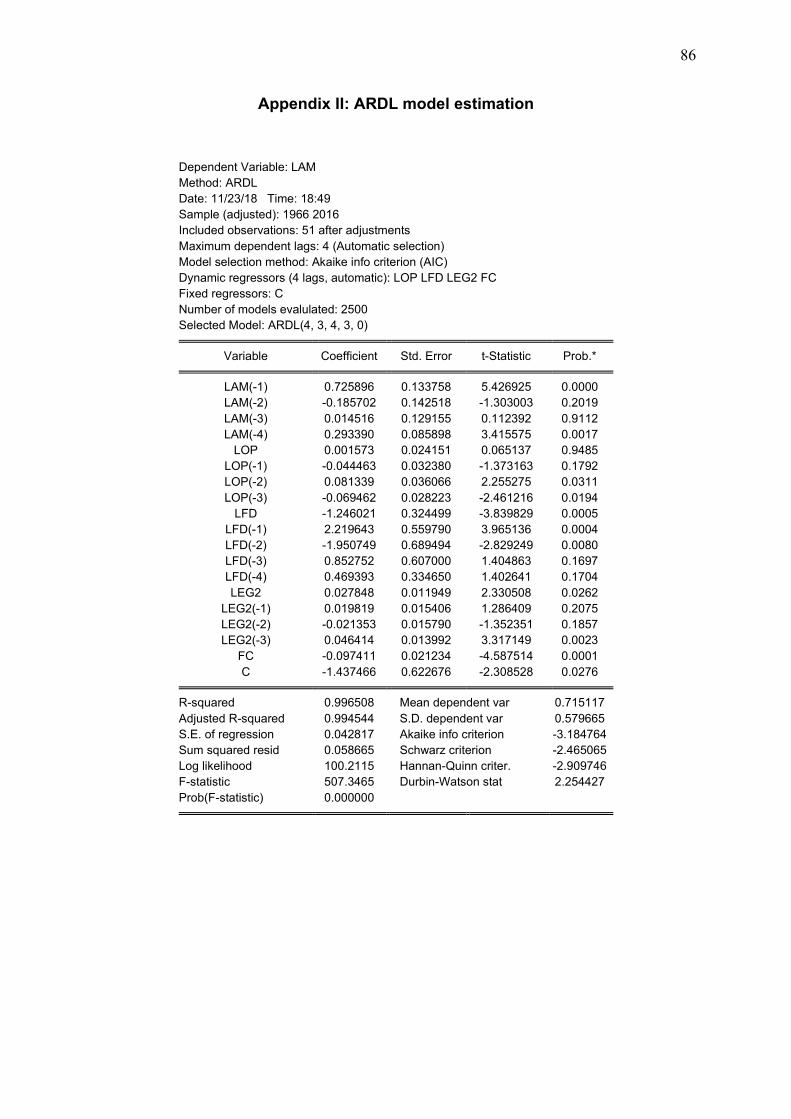
86
Appendix II: ARDL model estimation
Dependent Variable: LAM
Method: ARDL
Date: 11/23/18 Time: 18:49
Sample (adjusted): 1966 2016
Included observations: 51 after adjustments
Maximum dependent lags: 4 (Automatic selection)
Model selection method: Akaike info criterion (AIC)
Dynamic regressors (4 lags, automatic): LOP LFD LEG2 FC
Fixed regressors: C
Number of models evalulated: 2500
Selected Model: ARDL(4, 3, 4, 3, 0)
Variable Coefficient Std. Error t-Statistic Prob.*
LAM(-1) 0.725896 0.133758 5.426925 0.0000
LAM(-2) -0.185702 0.142518 -1.303003 0.2019
LAM(-3) 0.014516 0.129155 0.112392 0.9112
LAM(-4) 0.293390 0.085898 3.415575 0.0017
LOP 0.001573 0.024151 0.065137 0.9485
LOP(-1) -0.044463 0.032380 -1.373163 0.1792
LOP(-2) 0.081339 0.036066 2.255275 0.0311
LOP(-3) -0.069462 0.028223 -2.461216 0.0194
LFD -1.246021 0.324499 -3.839829 0.0005
LFD(-1) 2.219643 0.559790 3.965136 0.0004
LFD(-2) -1.950749 0.689494 -2.829249 0.0080
LFD(-3) 0.852752 0.607000 1.404863 0.1697
LFD(-4) 0.469393 0.334650 1.402641 0.1704
LEG2 0.027848 0.011949 2.330508 0.0262
LEG2(-1) 0.019819 0.015406 1.286409 0.2075
LEG2(-2) -0.021353 0.015790 -1.352351 0.1857
LEG2(-3) 0.046414 0.013992 3.317149 0.0023
FC -0.097411 0.021234 -4.587514 0.0001
C -1.437466 0.622676 -2.308528 0.0276
R-squared 0.996508 Mean dependent var 0.715117
Adjusted R-squared 0.994544 S.D. dependent var 0.579665
S.E. of regression 0.042817 Akaike info criterion -3.184764
Sum squared resid 0.058665 Schwarz criterion -2.465065
Log likelihood 100.2115 Hannan-Quinn criter. -2.909746
F-statistic 507.3465 Durbin-Watson stat 2.254427
Prob(F-statistic) 0.000000
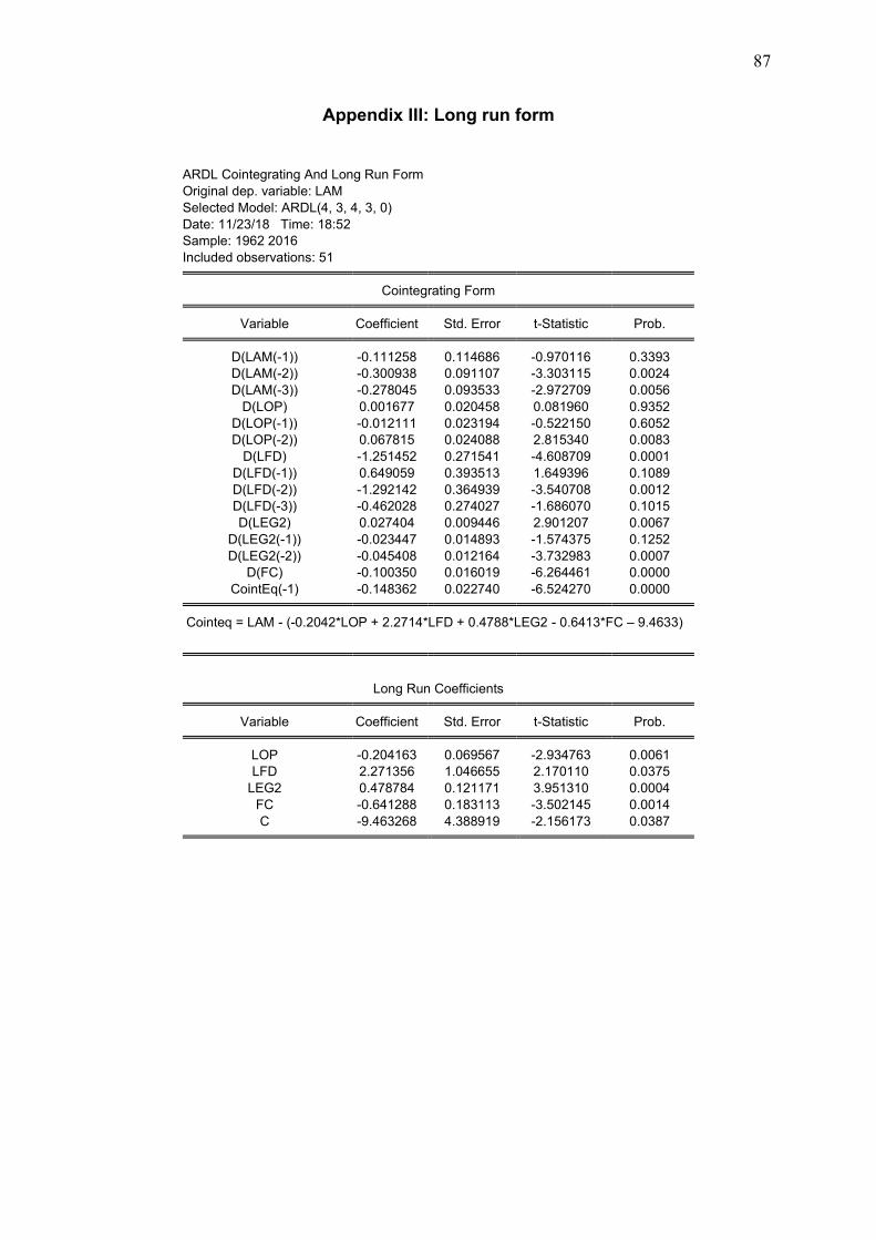
87
Appendix III: Long run form
ARDL Cointegrating And Long Run Form
Original dep. variable: LAM
Selected Model: ARDL(4, 3, 4, 3, 0)
Date: 11/23/18 Time: 18:52
Sample: 1962 2016
Included observations: 51 Cointegrating Form Variable Coefficient Std. Error t-Statistic Prob. D(LAM(-1)) -0.111258 0.114686 -0.970116 0.3393
D(LAM(-2)) -0.300938 0.091107 -3.303115 0.0024
D(LAM(-3)) -0.278045 0.093533 -2.972709 0.0056
D(LOP) 0.001677 0.020458 0.081960 0.9352
D(LOP(-1)) -0.012111 0.023194 -0.522150 0.6052
D(LOP(-2)) 0.067815 0.024088 2.815340 0.0083
D(LFD) -1.251452 0.271541 -4.608709 0.0001
D(LFD(-1)) 0.649059 0.393513 1.649396 0.1089
D(LFD(-2)) -1.292142 0.364939 -3.540708 0.0012
D(LFD(-3)) -0.462028 0.274027 -1.686070 0.1015
D(LEG2) 0.027404 0.009446 2.901207 0.0067
D(LEG2(-1)) -0.023447 0.014893 -1.574375 0.1252
D(LEG2(-2)) -0.045408 0.012164 -3.732983 0.0007
D(FC) -0.100350 0.016019 -6.264461 0.0000
CointEq(-1) -0.148362 0.022740 -6.524270 0.0000 Cointeq = LAM - (-0.2042*LOP + 2.2714*LFD + 0.4788*LEG2 - 0.6413*FC – 9.4633)
Long Run Coefficients Variable Coefficient Std. Error t-Statistic Prob. LOP -0.204163 0.069567 -2.934763 0.0061
LFD 2.271356 1.046655 2.170110 0.0375
LEG2 0.478784 0.121171 3.951310 0.0004
FC -0.641288 0.183113 -3.502145 0.0014
C -9.463268 4.388919 -2.156173 0.0387
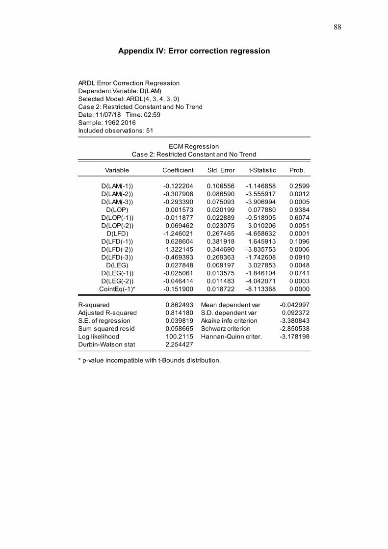
88
Appendix IV: Error correction regression
ARDL Error Correction Regression
Dependent Variable: D(LAM)
Selected Model: ARDL(4, 3, 4, 3, 0)
Case 2: Restricted Constant and No Trend
Date: 11/07/18 Time: 02:59
Sample: 1962 2016
Included observations: 51
ECM Regression
Case 2: Restricted Constant and No Trend
Variable Coefficient Std. Error t-Statistic Prob.
D(LAM(-1)) -0.122204 0.106556 -1.146858 0.2599
D(LAM(-2)) -0.307906 0.086590 -3.555917 0.0012
D(LAM(-3)) -0.293390 0.075093 -3.906994 0.0005
D(LOP) 0.001573 0.020199 0.077880 0.9384
D(LOP(-1)) -0.011877 0.022889 -0.518905 0.6074
D(LOP(-2)) 0.069462 0.023075 3.010206 0.0051
D(LFD) -1.246021 0.267465 -4.658632 0.0001
D(LFD(-1)) 0.628604 0.381918 1.645913 0.1096
D(LFD(-2)) -1.322145 0.344690 -3.835753 0.0006
D(LFD(-3)) -0.469393 0.269363 -1.742608 0.0910
D(LEG) 0.027848 0.009197 3.027853 0.0048
D(LEG(-1)) -0.025061 0.013575 -1.846104 0.0741
D(LEG(-2)) -0.046414 0.011483 -4.042071 0.0003
CointEq(-1)* -0.151900 0.018722 -8.113368 0.0000
R-squared 0.862493 Mean dependent var -0.042997
Adjusted R-squared 0.814180 S.D. dependent var 0.092372
S.E. of regression 0.039819 Akaike info criterion -3.380843
Sum squared resid 0.058665 Schwarz criterion -2.850538
Log likelihood 100.2115 Hannan-Quinn criter. -3.178198
Durbin-Watson stat 2.254427
* p-value incompatible with t-Bounds distribution.

89
Appendix V: Bounds test
ARDL Long Run Form and Bounds Test
Dependent Variable: D(LAM)
Selected Model: ARDL(4, 3, 4, 3, 0)
Case 2: Restricted Constant and No Trend
Date: 11/07/18 Time: 02:41
Sample: 1962 2016
Included observations: 51
F-Bounds Test Null Hypothesis: No levels relationship
Test Statistic Value Signif. I(0) I(1)
Asymptotic: n=1000
F-statistic 9.488540 10% 2.2 3.09
k 4 5% 2.56 3.49
2.5% 2.88 3.87
1% 3.29 4.37
Actual Sample Size 51 Finite Sample: n=55
10% 2.345 3.28
5% 2.763 3.813
1% 3.738 4.947
Finite Sample: n=50
10% 2.372 3.32
5% 2.823 3.872
1% 3.845 5.15

90
Appendix VI: Log likelihood test
Redundant Variables Test
Null hypothesis: LOP LFD LEG2 FC are jointly insignificant
Equation: UNTITLED Specification:
LAM LAM(-1) LAM(-2) LAM(-3) LAM(-4) LOP LOP(-1) LOP(-2) LOP(-3) LFD LFD(-1) LFD(-2) LFD(-3) LFD(-4) LEG2 LEG2(-1) LEG2(-2) LEG2(-3) FC C
Redundant Variables: LOP LFD LEG2 FC Value df Probability
F-statistic 14.33562 (4, 32) 0.0000 F-test summary:
Sum of Sq. df Mean
Squares
Test SSR 0.105125 4 0.026281
Restricted SSR 0.163790 36 0.004550
Unrestricted SSR 0.058665 32 0.001833
Restricted Test Equation:
Dependent Variable: LAM
Method: Least Squares
Date: 11/23/18 Time: 18:58
Sample: 1966 2016
Included observations: 51 Variable Coefficient Std. Error t-Statistic Prob. LAM(-1) 1.035931 0.180818 5.729132 0.0000
LAM(-2) -0.167682 0.215890 -0.776699 0.4424
LAM(-3) -0.254939 0.194238 -1.312509 0.1977
LAM(-4) 0.312289 0.131765 2.370049 0.0233
LOP(-1) -0.105127 0.034107 -3.082287 0.0039
LOP(-2) 0.163146 0.052309 3.118865 0.0036
LOP(-3) -0.086751 0.040979 -2.116991 0.0412
LFD(-1) 1.307867 0.571991 2.286516 0.0282
LFD(-2) -2.528764 1.007968 -2.508774 0.0168
LFD(-3) 0.848704 0.935681 0.907044 0.3704
LFD(-4) 0.997867 0.503487 1.981912 0.0552
LEG2(-1) -0.024199 0.019673 -1.230058 0.2267
LEG2(-2) -0.047769 0.022051 -2.166317 0.0370
LEG2(-3) 0.055269 0.020892 2.645493 0.0120
C -2.507262 0.894057 -2.804365 0.0081 R-squared 0.990251 Mean dependent var 0.715117
Adjusted R-squared 0.986460 S.D. dependent var 0.579665
S.E. of regression 0.067452 Akaike info criterion -2.314886
Sum squared resid 0.163790 Schwarz criterion -1.746702
Log likelihood 74.02959 Hannan-Quinn criter. -2.097766
F-statistic 261.1909 Durbin-Watson stat 2.171323
Prob(F-statistic) 0.000000
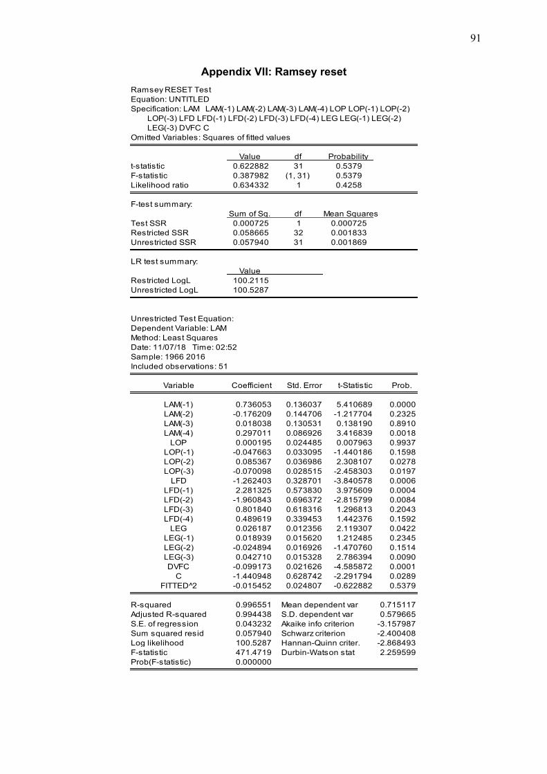
91
Appendix VII: Ramsey reset
Ramsey RESET Test
Equation: UNTITLED
Specification: LAM LAM(-1) LAM(-2) LAM(-3) LAM(-4) LOP LOP(-1) LOP(-2)
LOP(-3) LFD LFD(-1) LFD(-2) LFD(-3) LFD(-4) LEG LEG(-1) LEG(-2)
LEG(-3) DVFC C
Omitted Variables: Squares of fitted values
Value df Probability
t-statistic 0.622882 31 0.5379
F-statistic 0.387982 (1, 31) 0.5379
Likelihood ratio 0.634332 1 0.4258
F-test summary:
Sum of Sq. df Mean Squares
Test SSR 0.000725 1 0.000725
Restricted SSR 0.058665 32 0.001833
Unrestricted SSR 0.057940 31 0.001869
LR test summary:
Value
Restricted LogL 100.2115
Unrestricted LogL 100.5287
Unrestricted Test Equation:
Dependent Variable: LAM
Method: Least Squares
Date: 11/07/18 Time: 02:52
Sample: 1966 2016
Included observations: 51
Variable Coefficient Std. Error t-Statistic Prob.
LAM(-1) 0.736053 0.136037 5.410689 0.0000
LAM(-2) -0.176209 0.144706 -1.217704 0.2325
LAM(-3) 0.018038 0.130531 0.138190 0.8910
LAM(-4) 0.297011 0.086926 3.416839 0.0018
LOP 0.000195 0.024485 0.007963 0.9937
LOP(-1) -0.047663 0.033095 -1.440186 0.1598
LOP(-2) 0.085367 0.036986 2.308107 0.0278
LOP(-3) -0.070098 0.028515 -2.458303 0.0197
LFD -1.262403 0.328701 -3.840578 0.0006
LFD(-1) 2.281325 0.573830 3.975609 0.0004
LFD(-2) -1.960843 0.696372 -2.815799 0.0084
LFD(-3) 0.801840 0.618316 1.296813 0.2043
LFD(-4) 0.489619 0.339453 1.442376 0.1592
LEG 0.026187 0.012356 2.119307 0.0422
LEG(-1) 0.018939 0.015620 1.212485 0.2345
LEG(-2) -0.024894 0.016926 -1.470760 0.1514
LEG(-3) 0.042710 0.015328 2.786394 0.0090
DVFC -0.099173 0.021626 -4.585872 0.0001
C -1.440948 0.628742 -2.291794 0.0289
FITTED^2 -0.015452 0.024807 -0.622882 0.5379
R-squared 0.996551 Mean dependent var 0.715117
Adjusted R-squared 0.994438 S.D. dependent var 0.579665
S.E. of regression 0.043232 Akaike info criterion -3.157987
Sum squared resid 0.057940 Schwarz criterion -2.400408
Log likelihood 100.5287 Hannan-Quinn criter. -2.868493
F-statistic 471.4719 Durbin-Watson stat 2.259599
Prob(F-statistic) 0.000000
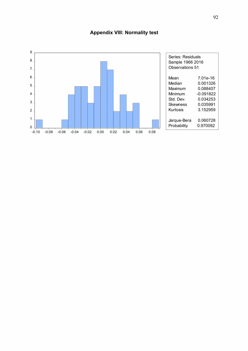
92
Appendix VIII: Normality test
0
1
2
3
4
5
6
7
8
9
-0.10 -0.08 -0.06 -0.04 -0.02 0.00 0.02 0.04 0.06 0.08
Series: Residuals
Sample 1966 2016
Observations 51
Mean 7.01e-16
Median 0.001326
Maximum 0.088407
Minimum -0.091822
Std. Dev. 0.034253
Skewness 0.035991
Kurtosis 3.152959
Jarque-Bera 0.060728
Probability 0.970092
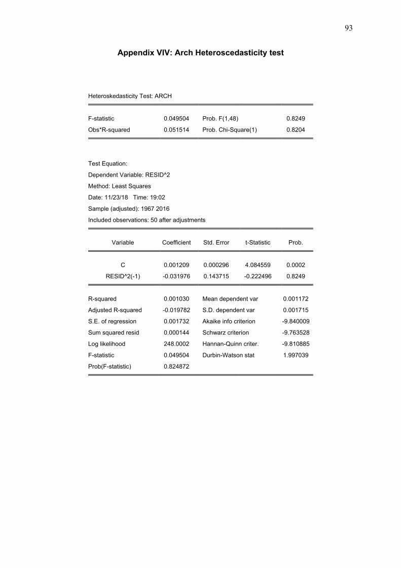
93
Appendix VIV: Arch Heteroscedasticity test
Heteroskedasticity Test: ARCH
F-statistic 0.049504 Prob. F(1,48) 0.8249
Obs*R-squared 0.051514 Prob. Chi-Square(1) 0.8204
Test Equation:
Dependent Variable: RESID^2
Method: Least Squares
Date: 11/23/18 Time: 19:02
Sample (adjusted): 1967 2016
Included observations: 50 after adjustments
Variable Coefficient Std. Error t-Statistic Prob.
C 0.001209 0.000296 4.084559 0.0002
RESID^2(-1) -0.031976 0.143715 -0.222496 0.8249
R-squared 0.001030 Mean dependent var 0.001172
Adjusted R-squared -0.019782 S.D. dependent var 0.001715
S.E. of regression 0.001732 Akaike info criterion -9.840009
Sum squared resid 0.000144 Schwarz criterion -9.763528
Log likelihood 248.0002 Hannan-Quinn criter. -9.810885
F-statistic 0.049504 Durbin-Watson stat 1.997039
Prob(F-statistic) 0.824872
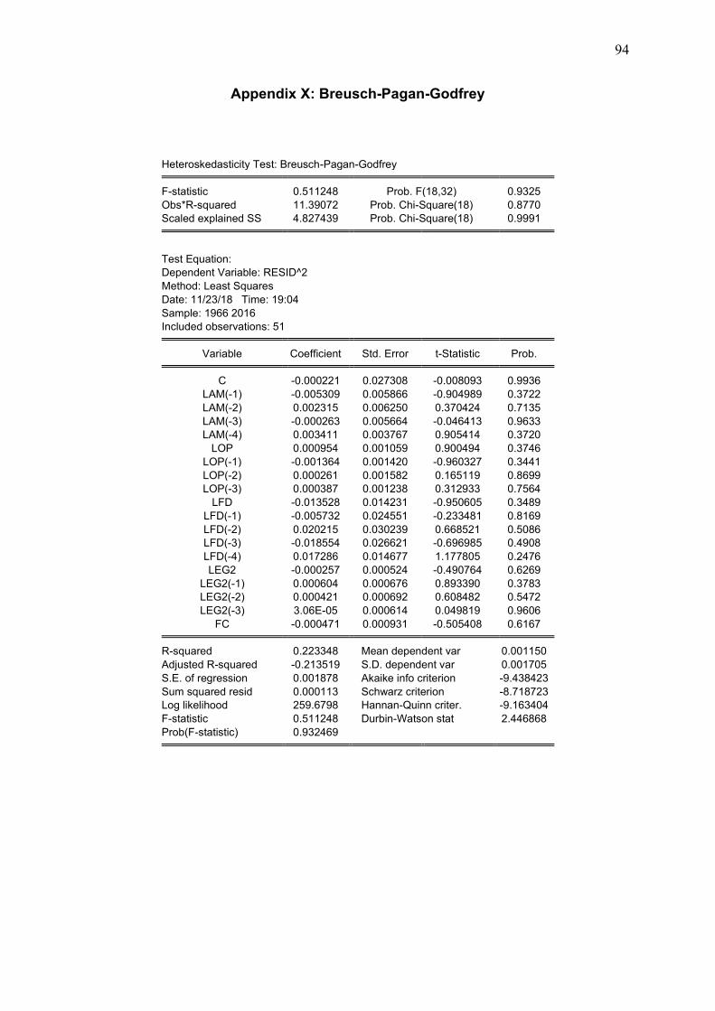
94
Appendix X: Breusch-Pagan-Godfrey
Heteroskedasticity Test: Breusch-Pagan-Godfrey F-statistic 0.511248 Prob. F(18,32) 0.9325
Obs*R-squared 11.39072 Prob. Chi-Square(18) 0.8770
Scaled explained SS 4.827439 Prob. Chi-Square(18) 0.9991
Test Equation:
Dependent Variable: RESID^2
Method: Least Squares
Date: 11/23/18 Time: 19:04
Sample: 1966 2016
Included observations: 51 Variable Coefficient Std. Error t-Statistic Prob. C -0.000221 0.027308 -0.008093 0.9936
LAM(-1) -0.005309 0.005866 -0.904989 0.3722
LAM(-2) 0.002315 0.006250 0.370424 0.7135
LAM(-3) -0.000263 0.005664 -0.046413 0.9633
LAM(-4) 0.003411 0.003767 0.905414 0.3720
LOP 0.000954 0.001059 0.900494 0.3746
LOP(-1) -0.001364 0.001420 -0.960327 0.3441
LOP(-2) 0.000261 0.001582 0.165119 0.8699
LOP(-3) 0.000387 0.001238 0.312933 0.7564
LFD -0.013528 0.014231 -0.950605 0.3489
LFD(-1) -0.005732 0.024551 -0.233481 0.8169
LFD(-2) 0.020215 0.030239 0.668521 0.5086
LFD(-3) -0.018554 0.026621 -0.696985 0.4908
LFD(-4) 0.017286 0.014677 1.177805 0.2476
LEG2 -0.000257 0.000524 -0.490764 0.6269
LEG2(-1) 0.000604 0.000676 0.893390 0.3783
LEG2(-2) 0.000421 0.000692 0.608482 0.5472
LEG2(-3) 3.06E-05 0.000614 0.049819 0.9606
FC -0.000471 0.000931 -0.505408 0.6167 R-squared 0.223348 Mean dependent var 0.001150
Adjusted R-squared -0.213519 S.D. dependent var 0.001705
S.E. of regression 0.001878 Akaike info criterion -9.438423
Sum squared resid 0.000113 Schwarz criterion -8.718723
Log likelihood 259.6798 Hannan-Quinn criter. -9.163404
F-statistic 0.511248 Durbin-Watson stat 2.446868
Prob(F-statistic) 0.932469
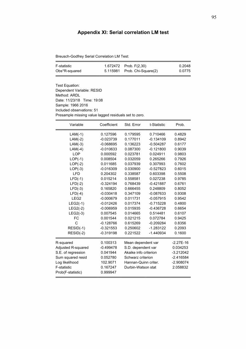
95
Appendix XI: Serial correlation LM test
Breusch-Godfrey Serial Correlation LM Test:
F-statistic 1.672472 Prob. F(2,30) 0.2048
Obs*R-squared 5.115981 Prob. Chi-Square(2) 0.0775
Test Equation:
Dependent Variable: RESID
Method: ARDL
Date: 11/23/18 Time: 19:08
Sample: 1966 2016
Included observations: 51
Presample missing value lagged residuals set to zero.
Variable Coefficient Std. Error t-Statistic Prob.
LAM(-1) 0.127596 0.179595 0.710466 0.4829
LAM(-2) -0.023739 0.177011 -0.134109 0.8942
LAM(-3) -0.068695 0.136223 -0.504287 0.6177
LAM(-4) -0.010633 0.087300 -0.121800 0.9039
LOP 0.000592 0.023781 0.024911 0.9803
LOP(-1) 0.008504 0.032059 0.265266 0.7926
LOP(-2) 0.011685 0.037939 0.307993 0.7602
LOP(-3) -0.016309 0.030900 -0.527823 0.6015
LFD 0.204302 0.338587 0.603398 0.5508
LFD(-1) 0.015214 0.558581 0.027238 0.9785
LFD(-2) -0.324194 0.768439 -0.421887 0.6761
LFD(-3) 0.165820 0.666455 0.248809 0.8052
LFD(-4) -0.030418 0.347109 -0.087633 0.9308
LEG2 -0.000679 0.011731 -0.057915 0.9542
LEG2(-1) -0.012426 0.017374 -0.715228 0.4800
LEG2(-2) -0.006959 0.015935 -0.436728 0.6654
LEG2(-3) 0.007545 0.014665 0.514481 0.6107
FC 0.001544 0.021215 0.072784 0.9425
C -0.128766 0.615269 -0.209284 0.8356
RESID(-1) -0.321553 0.250602 -1.283122 0.2093
RESID(-2) -0.319198 0.221522 -1.440934 0.1600
R-squared 0.100313 Mean dependent var -2.27E-16
Adjusted R-squared -0.499478 S.D. dependent var 0.034253
S.E. of regression 0.041944 Akaike info criterion -3.212042
Sum squared resid 0.052780 Schwarz criterion -2.416584
Log likelihood 102.9071 Hannan-Quinn criter. -2.908074
F-statistic 0.167247 Durbin-Watson stat 2.058832
Prob(F-statistic) 0.999947

96
SIMILARITY INDEX
97
ETHICAL APPROVAL
BİLİMSEL ARAŞTIRMALAR ETİK KURULU
25.10.2018
Sayın Simbarashe Rabson Andrea
Bilimsel Araştırmalar Etik Kurulu’na yapmış olduğunuz “The Nexus Between
Agricultural Productivity, Oil Prices, Financial Development And Economic
Growth In Usa” başlıklı proje önerisi, sadece ikincil kaynak kullanıldığı için Etik
Kuruluruna girmesine gerek yoktur. Bu yazı ile birlikte sadece ikincil kaynak kullanmak
şartıyla araştırmaya başlayabilirsiniz.
Doçent Doktor Direnç Kanol
Bilimsel Araştırmalar Etik Kurulu Raportörü
Not: Eğer bir kuruma resmi bir kabul yazısı sunmak istiyorsanız, Yakın Doğu
Üniversitesi Bilimsel Araştırmalar Etik Kurulu’na bu yazı ile başvurup, kurulun
başkanının imzasını taşıyan resmi bir yazı temin edebilirsiniz.
98
BİLİMSEL ARAŞTIRMALAR ETİK KURULU
25.10.2018
Dear Simbarashe Rabson Andrea
Your project “The Nexus Between Agricultural Productivity, Oil Prices, Financial
Development And Economic Growth In Usa " has been evaluated. Since only
secondary data will be used the project it does not need to go through the ethics
committee. You can start your research on the condition that you will use only
secondary data.
Assoc. Prof. Dr. Direnç Kanol
Rapporteur of the Scientific Research Ethics Committee
Note:If you need to provide an official letter to an institution with the signature of the
Head of NEU Scientific Research Ethics Committee, please apply to the secretariat of
the ethics committee by showing this document.