_____________________________________________________________________

CREDIT Research Paper

No. 15/07

_____________________________________________________________________

The Nature of Agricultural Markets:

Output Marketing in Tanzania

by

Basile Boulay

Abstract

This paper uses the three available waves of data from the Tanzanian National Panel Surveys

to study different agricultural markets. We use crop level data to analyse the factors

influencing farmers’ choice between selling to market or retaining output for household

consumption, allowing for market differences across crops. We estimate probit models for

each wave and crop (or crop categories). Results show that there is not a homogeneous

market for all crops, and the entrance decision is driven by different factors.

Contemporaneous and lagged prices as well as use of storage facility are important variables

that influence the decision to enter a market differently across crops. Entering the markets for

subsistence crops such as maize or cassava can be the result of economic distress, supporting

a ‘forced commerce’ hypothesis. The market for export crops responds to price and

expectation mechanisms and is closer to the conception of agricultural markets in standard

theory.

JEL Classification: Q12, Q13, R20, O13

Keywords: Agricultural economics, Tanzania, applied econometrics, crop sales

_____________________________________________________________________

Centre for Research in Economic Development and International Trade,

University of Nottingham

_____________________________________________________________________

CREDIT Research Paper

No. 15/07

The Nature of Agricultural Markets:

Output Marketing in Tanzania by

Basile Boulay

Outline

1. Introduction

2. Agriculture in Tanzania

3. Background and methodological issues

4. Summary statistics and estimation strategy

5. Empirical results

6. Discussion and conclusions

References

Appendices

The Author

Basile Boulay is a PhD student in the School of Economics at the University of

Nottingham. Email: lexbb6@nottingham.ac.uk

Acknowledgements

The author is grateful to Professor Oliver Morrissey and Dr Sarah Bridges for their

useful comments and support. He is grateful to the ESRC for PhD funding as a DTC

student.

_____________________________________________________________________

Research Papers at www.nottingham.ac.uk/economics/credit/

1

1. Introduction

Frequent national plans and strategies have been launched to stimulate the agricultural

sector and intensify cultivations in Tanzania. Most plans since 2000 (such as the

Agricultural Sector Development Strategy, ASDS, or the Agricultural Sector Development

Program, ASDP), are part of a more encompassing national plan named National

Development Visions 2025, which aims at transforming Tanzania into a semi-

industrialised economy with a productive agricultural sector by that year (Leyaro and

Morrissey, 2013).

Despite agriculture being officially at the top of the political agenda, there is no

comprehensive study of national patterns of production and output marketing in

Tanzania using the recent National Panel Surveys (NPS). This paper aims at bridging

this gap by studying output marketing for the main crops and categories of crops in

Tanzanian agriculture, using the three available NPS waves (2008/2009, 2010/2011

and 2012/2013). The analysis aims at determining the factors that push farmers to

enter the market for particular crops (or category of crops). Probit models are

estimated at the crop (category) level. The main contribution is to show that the nature

of the markets fundamentally differs across crops, thus making the point that markets

are institutional structures that vary across crops. In particular, it is shown that the

rationales for entering the markets differ across crops, and that the socio-economic

factors associated with selection into the market are not homogeneous. A key result is

that there is no such thing as ‘the’ agricultural market. Rather, there are many

agricultural markets, each shaped by particular specificities.

The structure of this paper is as follows: section 2 reviews the literature on the

agricultural sector in Tanzania and historical evolution. Section 3 provides a

methodological background to the question. Section 4 presents the data sources and

explains the main challenges the data presents. Section 5 reports results on the

determinants of entering the markets for different crops and goodness of fit analysis.

Section 6 presents the main conclusions and directions for future work.

2. Agriculture in Tanzania

Agriculture has been at the centre of political strategies in Tanzania since independence

in 1961. The signing of the Arusha Declaration in 1967 symbolised the consolidation of

the party of the Revolution (CCM) and its charismatic leader Nyerere. The declaration

stressed the virtues of self-reliance as opposed to dependence upon foreign aid (in

particular by pervious colonial powers). Agriculture was the main channel Nyerere

envisaged to achieve self-reliance. Referred to as Ujamaa, farming communities were

created, often through (forced) villagisation policies, in order to foster specialisation

and offer a more efficient resources provision.

2

Today, while it is generally recognized that Ujamaa did not meet expectations and had

numerous negative side-effects, the ‘agricultural question’ is still central in Tanzania,

and the sector is going through a prolonged period of stagnation. Following Ujamaa

(and Nyerere’s withdrawal of power in 1985), a period of structural adjustment and

market-friendly reforms were implemented, with heavy involvement of the IMF and

World Bank (despite the initial support to Ujamaa by the World Bank). The dismantling

of parastatals, removal of price marketing boards, progressive removal of inorganic

fertiliser subsidies, were all measures aimed at ‘getting prices right’ and providing

farmers with the ‘right’ incentives that would stimulate productivity and specialisation.

Whilst Ujamaa did not meet expectations, it is clear that liberalisation did not deliver

what it promised either (Skarstein, 2005).

The literature on recent performance of Tanzanian agriculture is relatively scarce. The

picture that emerges is that liberalisation has not lived up to its promises, at least not to

the extent that it was expected to in the aftermath of Ujamaa policies. A useful recap of

the timing of events is provided in Isinika et al (2011), with the ‘shift’ occurring in two

stages: heavy market reforms during the 1980s to ‘get the prices right’, followed by a

decade that reflected the growing importance in standard economics of ‘getting the

Institutions right’, largely shaped by the work of New-Institutionalist economists. Thus,

apart from the dismantling of parastatals and removal of input subsidies associated

with market reforms, Institutional reforms were also implemented. A major

cornerstone of those reforms was the Land policy of 1995 and Land laws of 1999, which

stressed the ‘intrinsic’ value of land, thus taking the normative stance that land markets

should exist. Ultimately, both market and institutional reforms aimed at increasing

farmers’ productivity through changing the incentives structure.

There is no consensus on the effects of adjustment, especially at the crop level.

According to Bryceson (2010), the phase of liberalisation was beneficial for cotton and

coffee in the 1990s, with harvests regularly exceeding historical averages. However, the

performance of the export sector today is still below the performance of the 1960s

when looking at the per capita volume of exports, particularly so for cashew nuts, an

important crop. Production of maize, the main staple crop, was greatly affected by

liberalisation. Skarstein (2010) and Isinika et al (2011) argue that the removal of

fertiliser subsidies made supply less available in the traditionally maize-producing

remote regions of the country (such as the Ruvuma or Rukwa regions). The outcome of

this was a large shift in maize producing regions from the remote Central and Western

regions towards either Central regions with strong commercial base (such as Dodoma),

or towards Northern regions which have more fertile land for maize (such as Arusha).

This is because, they argue, liberalisation fundamentally changed the structures of

farming profitability because of the changing costs for inputs and transport. Skarstein

(2010) reports that over 1985-1998 (i.e., the liberalisation period), maize production in

per capita terms fell by 22.5%. McKay et al (1997) have argued that liberalisation did

not deliver its promises for several reasons. The first is that the change in incentive

3

structures supposed to promote exports mainly affected the manufacturing sector.

Second, a crucial condition for liberalisation is that farmers should have access to inputs

and credit. In the case of Tanzania, access to fertiliser clearly declined. Thirdly, fallacy

compositions can arise if similar countries liberalise at the same time, creating

increases in supply on world markets pushing prices down.

In this context, it was argued that liberalisation policies neglected certain elements that

were needed for a successful transformation. In particular, access to credit, inputs,

better infrastructure etc. were considered to be important factors that liberalisation had

not delivered properly. This led to what Isinika et al (2011) refer to as ‘policy reversal’,

which is somewhat misleading in the sense that the aim was to complement

liberalisation rather than reverse back to pre-liberalisation policies. The main changes

were the re-introduction of subsidies for inputs, which can be justified in both efficiency

and equity grounds (Minot and Benson, 2009). A voucher input system was recently

launched in 2008 as part of the public strategy for agricultural development. The NAIVS

(National Agricultural Input Voucher Scheme) provided subsidies for maize and paddy

rice in form of a 50% discount on fertiliser and seeds for farmers, conditional on them

being able to ‘top-up’ the remaining 50% of the price (Malhorta, 2013). Another feature

of liberalisation is that it has largely increased price volatility (Barret, 2008 and

Skarstein 2010) for poor farmers. Barrett argues that liberalisation has pushed many

farmers back into subsistence due to the large spot market price volatility.

As a result, one of the crucial features in today’s agricultural sector is that output

growth is largely driven by extensification rather than intensification. There is no

evidence that fertiliser usage is increasing over time (if anything, slight decreases are

observed). Growth seems to take place through land expansion (Kirchberger and

Mishili, 2011). This expansion is usually carried through clearing patches of forest land,

which are often not as fertile as arable land, and constitute a real ecological and

livelihood issue for the country. Therefore, it is crucial to assess the potential for

intensification in Tanzanian agriculture. Although referring to neighbouring countries,

Jayne et al (2010) argue that the issue of land is very rapidly changing in East Africa due

to population pressure, and that land should no longer be considered as an ‘unlimited’

factor as it has often been in the past. Looking at the Katoro-Buserere area in Northern

Tanzania, Bryceson (2010) reports anthropological evidence of growing land scarcity

and the emergence of a landless class of farmers, affecting young generations mostly.

In that context, it is crucial to understand what are the factors pushing farmers to enter

(or refrain from entering) the market. While the production side must be studied to

understand what determines production, the sales side must be studied to identify

economic behaviour of farmers. Studying the latter is also highly relevant from a policy

perspective, since price and non-price factors influencing market participation are key

elements of any agricultural policy. In case of large differences in the nature of markets

across crops, such differences must also be accounted for by policies.

4

3. Background and methodological issues

While production per se is determined by physical factors, it is generally accepted that

selling this production is to a large extent based on farmers’ characteristics (age,

education etc.) as well as the economic environment (infrastructure, existence of a

market nearby etc.). Therefore, it is often posited that selection into the market is non-

random and depends on socio-economic characteristics of peasants, themselves

associated to market failures. Farmers’ education, access to capital and certain inputs,

social capital and proximity with different networks are considered to be key

determinants in farmers’ participation in the market. As such, sales behaviour is often

modelled as a sample selection issue, with a Heckman selection model. It is assumed

that farmers self-select into marketing output.

From a theoretical perspective, selection into markets is often seen as a problem

grounded in transaction cost theories. High transaction costs are associated with

market failures, particularly in SSA countries. Many transactions fail to take place

because of an array of causes related to these failures: poor infrastructures, little access

to information, or credit constraints to name just a few. The conventional view in

standard theory is that market failures inhibit farmers’ ability to respond to incentives,

in particular price incentives. De Janvry et al (1991) offer a classic account of this view

on market selection. They argue that market failures in rural economies are household

specific, rather than commodity specific (with labour being included as a ‘commodity’).

According to them, as market failures increase, the resulting price bands within which

peasant households do not sell increase, thus reducing the likelihood for those

households to enter the market: self-sufficiency becomes a more advantageous option

than engaging in the trading of factors (labour) or goods (agricultural output). These

price bands are an increasing function of the gap between the price at which peasant

households can sell factors or goods and that at which they can buy them (i.e. as market

failures increase).

Many empirical papers follow this theoretical approach of transaction costs affecting

market participation. A good example is the paper by Heltberg and Tarp (2002),

studying supply response of farmers in Mozambique. Following Key et al (2000), they

argue that marketing output involves two types of costs: fixed costs and variable

proportional transaction costs. While participation into the market (i.e., positive

selection) is determined by both fixed and variable costs, the quantity supplied only

depends on the latter. As a result, fixed transaction costs can be seen as the necessary

exclusion restrictions needed in the selection equation of a Heckman selection model.

According to Heltberg and Tarp (2002, p.107): ‘Measures of distance and transport are

expected to influence variable transaction costs, whereas information variables affect

fixed transaction costs’. As such, they consider the following variable transaction costs

measures: a dummy for ownership of transport, and the log of distances to the nearest

railway station and the provincial capital. For fixed transaction costs, they use a dummy

5

variable for ownership of TV/radio/phone, the maximum education of head of

household, and district population density.

Given available information in the Tanzanian surveys, the following related measures

are constructed (population density at the district level is not available from the

datasets):

For fixed transaction costs:

Dummies for whether farmers frequently listen to the radio, and frequently read

newspapers (coded as 0 if the answer is ‘never’ or ‘a few times a year only’, and 1

if the answer is ‘several times a month’ or ‘almost every day’).

Educational level of household head.

For variable transaction costs:

The (log) distance, in Km, to the closest market. Since the focus is at the crop

level, this measure is the average distance across plots.

A dummy for transport ownership (owning at least one of: bicycle, motorbike,

motor vehicle).

Four additional ‘exclusion restriction’ variables are considered. Availability of improved

seeds in the nearest village captures local level of technology and any commercial

integration effect, with the village being part of trading networks. The presence of a

farmers’ cooperative within the village captures networks effects, informational effect

and the possibility for farmers to gather information regarding marketing practices. It

may increase bargaining power of small-holders who do sell their output; Barrett

(2008) notes the recent resurgence of farmers’ cooperatives, partly as a result of

processes of liberalisation which often created large price volatility in output prices.

The third variable is whether anyone in the household is member of a saving or credit

group (the so-called ‘SACCOS’). This is expected to have an ambiguous effect. On the one

hand, this clearly implies better access to capital and formal saving/lending institutions,

which may facilitate selection into marketing some crops. On the other hand, it could

reflect the fact that the household is ‘disengaging’ from agriculture (or at least, from

output marketing) relative to households in which no one is a member of a saving

group. One possible reason is that members of saving groups may be individuals

employed in a formal job living in a household less reliant on agricultural production

than other households. Finally, whether a household uses a storage facility is

considered. This may proxy knowledge about prices and account for expectation

mechanisms. Each of these variables has a clear rationale for affecting selection into

agricultural markets.

Heltberg and Tarp (2002) only considers total farm sales, and therefore does not

account for crop specificities. In practice, it is of interest to understand which crops are

easily marketable, which are not, and to see which factors for which crops may push

6

farmers to participate in the market. For example, since some crops like cassava are

typical of subsistence or ‘back-up’ farming practices, one should not expect access to

capital or credit to be strongly linked with market participation. On the other hand,

crops such as coffee, which are mainly exported, require a minimum level of integration

into commercial network, as well as a certain degree of risk management, given that

coffee trees need several years before they reach maturity and harvests can be realised.

This implies that modelling selection at the aggregate level, while picking up the

importance of some socio-economic characteristics, will miss on the interactions

between those factors and the particularities of each crop (or types of crops).

Heckman selection models are not estimated here for a number of reasons. The main

aim is to understand what drives farmers to market a particular crop. While Heckman

models ask the question “conditional on selection into the market, what influences the

amount supplied by farmers?”, the question of interest here is “what are the factors that

push farmers to enter the markets?”. Too much attention in the literature has been given

to quantity equations corrected for selection, without questioning in depth the

rationales for entering markets. More importantly, it is implicitly assumed that ‘the

market’ is a homogeneous institutional structure and that entering it is the natural

result of commercial integration from the ‘more efficient’ farmers (as opposed to less

efficient small-scale/subsistence farmers). This partly stems from the fact that papers

often look either at aggregate agricultural outputs (thus blurring crop specificities) or

only at a given crop category, usually cereals or maize.

The processes of selection should be given equal attention. Before estimating selection-

corrected quantity equations, one should have an idea of the nature of the market for

each crop. There is no a priori reason to assume that entering the market is the same

process across crops. To reflect this, probit models are estimated for a large set of crops

and categories of crops. For each wave, a probit model is estimated including (among

others) the variables used by Heltberg and Tarp (2002) and the additional four

variables mentioned above (cooperative, saving groups, improved seeds and use of

storage). Note that since the focus is at the crop level, both sales and harvests are given

at the crop/farm level (i.e., across plots). This allows identifying which factors influence

farmers’ decisions to sell output for which crops.

4. Summary statistics and estimation strategy

4.1. Summary statistics and data construction

The datasets used in this study come from the three available waves of data of the

Tanzanian National Panel Surveys (NPS) for the years 2008/2009, 2010/2011 and

2012/2013. Despite the very rich information these datasets contain, their use has been

relatively scarce so far. These surveys are representative of the national population and

cover all regions. The NPSs are integrated household surveys, and as such, contain very

7

detailed information on agricultural production for households involved in the

agricultural sector. The agricultural questionnaire provides valuable information

regarding farming practices, agricultural production, and different types of inputs.

Appendix 1 provides details on data construction for the price and storage variables as

well as some stylized examples explaining specific features of the data and detailed

summary tables.

Most farmers do not market any of their agricultural output, indicating the possibility of

widespread subsistence farming. Further, it seems that large differences in marketing

behaviour are linked with the patterns of adoption of variable inputs (hired labour and

chemical fertiliser). Farmers using variable inputs seem more likely to engage in

marketing output than farmers not using any variable inputs. We therefore create the

following 4 categories of farming households:

Group 1: farmers not using any variable inputs. These are assumed to be

households most engaged in subsistence farming and home-consumption of

output. They represent the majority of farmers

Group 2: farmers only hiring labour (i.e., not using chemical fertiliser)

Group 3: farmers only using chemical fertiliser (i.e., not hiring labour)

Group 4: farmers hiring labour and using chemical fertiliser

Descriptive statistics are presented below for wave 1 for the main variables for groups 1

and 4, which are the two groups expected to be most different from each other. Results

for waves 2 and 3 are reported in appendix 1. The variable seller gives the proportion of

households selling at least part of output for one crop (i.e., if a farmer grows 2 crops but

only markets one, he is classified as a seller). This allows identifying the proportion of

farmers engaged in total subsistence with no market interaction at all.

Table 1: summary statistics: gr.1 wave 1

mean sd min max

Harvest (kg) 309 632.5 1 8800

Surplus (%) 0.21 0.3 0 1

Seller (0/1) 0.74 - 0 1

Price (TS) 308 294.3 2 3000

Sales (kg) 136 627.6 0 15000

Sales (TS) 30574 104482.8 0 1.90e+06

Family (days) 95 93.0 0 760

Organic fert (kg) 39 181.3 0 2000

N 4681

8

Table 2: summary statistics: gr4 wave 1

These tables show that average harvest is much higher among group 4 than group 1 (83

% higher), which is expected. In terms of average farm-gate price, group 1 is clearly

dominated in wave 1 (but experiences very strong increase in subsequent waves, see

appendix 1). Although the surplus (the proportion of output which is marketed) is, as

expected, higher for group 4 it is not markedly so. This may be a preliminary indicator

that self-sufficiency in some crops can be an endeavour for farmers across groups. In

wave 1, family labour is much more prevalent among farmers in group 1 (but this is not

the case for wave 3, see appendix 1). An interesting variable to look at is usage of

organic fertiliser, since it is often taken to be a proxy for animal power in the literature.

These summary statistics show a very high gap between groups 1 and 4 regarding usage

of manure. This may be a preliminary indicator that animal power (wealth) is much

greater in group 4 than among farmers in group 1 (this effect is observed in all waves).

The set of graphs below plots usage of fixed inputs across groups and waves. The blue

bar gives average number of days of family labour used per plot (fixed input), while the

red one gives the number of days of hired labour per plot (variable input). The green

bar shows the average amount or organic fertiliser used on a plot in Kgs (fixed input),

while the orange bar gives the amount of inorganic fertiliser used on a plot in Kgs

(variable input).

mean sd min max

Harvest (kg) 566 1018.4 1 9500

Surplus (%) 0.30 0.4 0 1

Seller (0/1) 0.82 - 0 1

Price (TS) 362 315.2 10 2500

Sales (kg) 508 3120.2 0 50880

Sales (TS) 1.09e+05 379319.5 0 3.41e+06

Family (days) 75 67.6 0 436

Organic fert (kg) 165 419.8 0 2000

Inorganic fert (kg) 90 128.3 1 800

Hired labour (days) 22 26.2 1 134

N 303

9

Graphs set 1: Inputs usage by waves and groups

The same picture does not emerge for the two fixed inputs. It is clear that organic

fertiliser usage is increasing across groups in all waves, possibly reflecting the fact that

as one move upwards across groups, farmers are less and less poor, which could be

proxied by animal power. However, family labour seems to be much more prevalent

across all groups. In wave 3, the mean appears very close across groups. One special

feature of group 4 is that across waves it clearly dominates all other groups in terms of

organic and group 3 in terms of inorganic fertiliser usage. On the other hand, note that

there is not much difference between groups 2 and 4 in terms of hired labour.

Regarding farm size, two counteracting factors may influence its evolution over time. On

the one hand, the (relative) absence of land market and reliance on customary law to

allocate land in most regions may imply that farm size decreases over time because

when households split land has to be reallocated between old and new households. On

the other hand, there is a general trend of area expansion. In particular, there is now

evidence that households expand their land by clearing patches of forest land to grow

crops. Excluding farms over 100 acres, average farm size is 4.9, 5.7 and 6.1 acres for

waves 1 to 3 respectively. Summary statistics by farmers groups reveal that this result

holds even for group 1. This is interesting because the summary statistics tables show

that average harvest is clearly declining over time. This can be explained by the fact that

area expansion is made into patches of forest which have very poor soil fertility,

reflecting a general trend of extensification rather than intensification.

10

However, the growth in farm size between waves 1 and 3 in group 1 has been much

slower than that for group 4 (21% against 59%). This growth rate for group 4 is quite

spectacular and suggests that very different patterns of land acquisition/accumulation

may be at work across different groups/types of farmers.

4.2. Estimation strategy

Probit models can be conceptualised in terms of an unobserved latent variable y* (in this

case, this can be the ‘net utility’ outcome from a cost-benefit analysis of entering versus

not entering a market). What we do observe is whether a farmer enters the market or

not:

{𝑦 = 1 𝑖𝑓 𝑦∗ > 0

𝑦 = 0 𝑖𝑓 𝑦∗ = 0 (𝟏)

A set of factors contained in vector x are believed to influence the decision to sell or

retain output, so that:

{𝑃(𝑌 = 1|𝒙) = 𝐹(𝒙, 𝛽)

𝑃 (𝑦 = 0|𝒙) = 1 − 𝐹(𝒙, 𝛽) (𝟐)

In the case of a probit model, F(.) is the standard normal distribution, so that:

𝑃(𝑌 = 1|𝒙) = Ф(𝒙′𝛽) (𝟑)

The model estimated is thus the following:

𝑃(𝑌 = 1|𝒙) = Ф (𝛼 + 𝛽1 log(ℎ𝑎𝑟𝑣𝑒𝑠𝑡)𝑖𝑐 + 𝛽2 log(𝑝𝑟𝑖𝑐𝑒)𝑖𝑐 + 𝛽3𝑔𝑟𝑜𝑢𝑝𝑖 + 𝛽4𝑟𝑒𝑔𝑖𝑜𝑛𝑖 + 𝜸 𝒊𝒏𝒑𝒖𝒕𝒊

+ 𝜹 𝑯𝑯𝒊 + θ 𝑑𝑖𝑠𝑡𝑎𝑛𝑐𝑒𝑖 + 𝜀𝑖𝑐) (𝟒)

The dependent variable is a binary outcome equal to 1 if household i sells crop c, and 0

otherwise. The error terms is assumed to have a normal distribution with mean zero.

Harvest represents realised harvest of a given crop across all plots on which that crop is

grown. The price regressor is farm gate price (either realized or imputed according the

method described in appendix 1). The group variable is a categorical variable with

group 1 as base group. The vector inputi is made of dummy variables for variables

inputs (inorganic fertiliser and hired labour) and fixed inputs (organic fertiliser and

family labour). These are dummies rather than continuous variables because inputs

usage is provided at the plot level. Therefore, it is impossible to match a given use of

inputs to a total crop harvest across plots (particularly when crops are intercropped).

The vector HHi is made of household level characteristics thought to influence market

selection: these are the variables considered by Heltberg and Tarp (2002), the

additional four variables created for the analysis (cooperative, storage use, saving group

11

and improved seeds), farm size, and whether the crops has been intercropped. The

variable on distance is the average plot distance for household i to the nearest village

market. Standard errors are clustered at the farm level to allow for correlation between

the sales of different crops within a same farm and estimation is made via maximum

likelihood.

Probits including lagged prices for waves 2 and 3 are estimated for comparison with the

baseline models. These augmented models ‘complement’ the baselines models but

suffer from the drawback of much lower sample sizes (including lagged prices requires

that farmers grow and market the same crop(s) in both waves). In those models,

equation 4 also includes lagged prices as a regressor. Table 3 shows the difference in

sample sizes at the aggregate level.

Table 3: Aggregate sample sizes with and without lagged prices1

For each crop, marginal effects are derived to study the importance on marketing

behaviour of the key regressors. Two different types of marginal effects can be obtained

from a probit: the average marginal effect (AME), and the marginal effect at the means

(MEM). The former calculates marginal effect for each observation in the data, and then

averages these effects out. The latter calculates the marginal effect at the average value

of the regressor considered. We follow Bartus (2005) in this paper by estimating AMEs

rather than MEMs on the grounds that AMEs are more realistic than MEMs.

The fit of estimated models is then carefully assessed through goodness of fit analysis.

Indeed, since the research focus is on whether households enter the market or not,

models should be good enough at distinguishing between sellers and non-sellers for

each crop studied.

5. Empirical results

5.1. Probit models at the crop/categories of crop level

For each crop, marginal effects for the main coefficients of interest are presented. The

full results from maximum likelihood estimation are reported in appendix 3. A

particularly important variable to look out in terms of marginal effects is the price

variable. Table 4 presents logs and corresponding price levels that are useful when

interpreting average marginal effects of prices.

1 Sample size refers to crops at the household level (ex. A household cultivating 3 crops on 5 plots would have 3 entries in the data altogether).

Wave 2 Wave 3

Sample size without lagged prices N=6878 (100%) N=9583 (100%)

Sample size with lagged prices N=3654 (53%) N=6950 (73%)

12

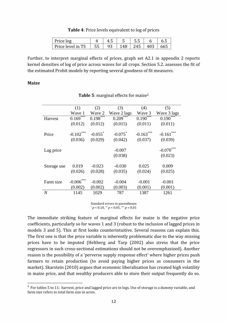
Table 4: Price levels equivalent to log of prices

Price log 4 4.5 5 5.5 6 6.5 Price level in TS 55 93 148 245 403 665

Further, to interpret marginal effects of prices, graph set A2.1 in appendix 2 reports

kernel densities of log of price across waves for all crops. Section 5.2. assesses the fit of

the estimated Probit models by reporting several goodness of fit measures.

Maize

Table 5: marginal effects for maize2

(1) (2) (3) (4) (5)

Wave 1 Wave 2 Wave 2 lags Wave 3 Wave 3 lags

Harvest 0.169***

0.198***

0.209***

0.190***

0.190***

(0.012) (0.012) (0.015) (0.011) (0.011)

Price -0.102***

-0.055* -0.075

* -0.163

*** -0.161

***

(0.036) (0.029) (0.042) (0.037) (0.039)

Lag price -0.007 -0.070***

(0.038) (0.023)

Storage use 0.019 -0.023 -0.030 0.025 0.009

(0.026) (0.028) (0.035) (0.024) (0.025)

Farm size -0.006***

-0.002 -0.004 -0.001 -0.001

(0.002) (0.002) (0.003) (0.001) (0.001)

N 1145 1029 787 1387 1261

Standard errors in parentheses * p < 0.10, ** p < 0.05, *** p < 0.01

The immediate striking feature of marginal effects for maize is the negative price

coefficients, particularly so for waves 1 and 3 (robust to the inclusion of lagged prices in

models 3 and 5). This at first looks counterintuitive. Several reasons can explain this.

The first one is that the price variable is inherently problematic due to the way missing

prices have to be imputed (Heltberg and Tarp (2002) also stress that the price

regressors in such cross-sectional estimations should not be overemphasized). Another

reason is the possibility of a ‘perverse supply response effect’ where higher prices push

farmers to retain production (to avoid paying higher prices as consumers in the

market). Skarstein (2010) argues that economic liberalisation has created high volatility

in maize price, and that wealthy producers able to store their output frequently do so.

2 For tables 5 to 11: harvest, price and lagged price are in logs. Use of storage is a dummy variable, and farm size refers to total farm size in acres.

13

Yet another reason is outlined in Barrett (2008): the poorest farmers are often net

buyers of the major staple crops, so that increases in prices may only benefit the

minority of large-scale and commercially integrated farmers, while hurting the rest of

them. This result is also consistent with Skarstein claim that ‘forced commerce’ is

widespread in Tanzania, understood as a process in which poor farmers are forced to

sell output at low prices after harvest to generate cash. Eventually, those poor

households run out of food before next harvest and are forced to buy food on the

market at much higher prices later in the year. In wave 3, both contemporaneous and

lagged prices have a negative effect on selection into the market. In wave 2, average unit

price for maize is 307TS, much higher than the average of 250TS for wave 1. In wave 3,

it is very high at 452TS. Therefore, if forced commerce is a plausible hypothesis, then it

is logical to observe a strongly negative cotemporaneous price in wave 3 (due to very

high selling price) and a negative lagged price, since prices in wave 2 were already

significantly higher than in wave 1. It is reassuring to see that the inclusion of lagged

prices does not alter the results significantly. The marginal effect of using a storage

facility is insignificant across waves, which is quite unexpected. Farm size does not

matter either, except for a small effect in wave 1. However, it represents the marginal

effect of increasing farm size by one acre (this does not refer to a one-acre increment in

area devoted to maize only, but to a one-acre increment of the total farm size), so that

small marginal effects are to be expected.

Marginal effects can also be calculated and plotted for different values of the regressors

of interest. Given the kernel densities for maize prices, it seems useful to look at

marginal effects of price between log(4) and log(6.4) (between 55 and 665TS).

Graphs 2: marginal effects of log of price for maize

This set of graphs show interesting insights. First, marginal effects of price are

invariably negatively affecting market selection, even at high price levels. Second this

effect gets smaller as price increases, especially for waves 1 and 3, both in terms of

magnitude and significance. This means that while higher selling price may hurt farmers

who are net buyers over the course of the year, this effect is mitigated as price strongly

increases. For maize, the kernel densities show high densities at log of 5.5 (245TS) for

waves 1 and 2 and log of 6 (403TS) for wave 3. For farmers facing those prices in waves

1 and 3, marginal effects of prices are significant and reduce the probability of not

14

selling output. In the third wave, for farmers facing unit prices below average, marginal

effects of price further increase the probability of not selling output. These farmers are

likely to be the poorest ones, and hence be hurt by price increases according to the

‘forced commerce hypothesis’.

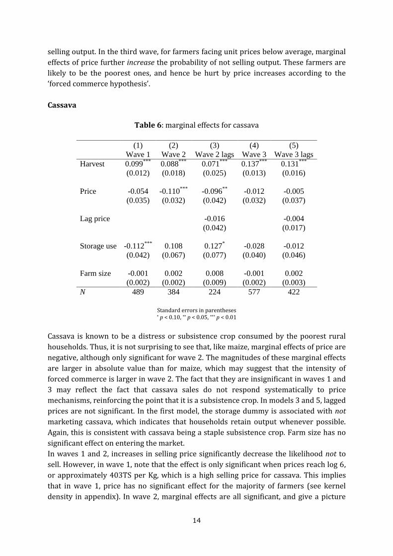
Cassava

Table 6: marginal effects for cassava

Standard errors in parentheses * p < 0.10, ** p < 0.05, *** p < 0.01

Cassava is known to be a distress or subsistence crop consumed by the poorest rural

households. Thus, it is not surprising to see that, like maize, marginal effects of price are

negative, although only significant for wave 2. The magnitudes of these marginal effects

are larger in absolute value than for maize, which may suggest that the intensity of

forced commerce is larger in wave 2. The fact that they are insignificant in waves 1 and

3 may reflect the fact that cassava sales do not respond systematically to price

mechanisms, reinforcing the point that it is a subsistence crop. In models 3 and 5, lagged

prices are not significant. In the first model, the storage dummy is associated with not

marketing cassava, which indicates that households retain output whenever possible.

Again, this is consistent with cassava being a staple subsistence crop. Farm size has no

significant effect on entering the market.

In waves 1 and 2, increases in selling price significantly decrease the likelihood not to

sell. However, in wave 1, note that the effect is only significant when prices reach log 6,

or approximately 403TS per Kg, which is a high selling price for cassava. This implies

that in wave 1, price has no significant effect for the majority of farmers (see kernel

density in appendix). In wave 2, marginal effects are all significant, and give a picture

(1) (2) (3) (4) (5)

Wave 1 Wave 2 Wave 2 lags Wave 3 Wave 3 lags

Harvest 0.099***

0.088***

0.071***

0.137***

0.131***

(0.012) (0.018) (0.025) (0.013) (0.016)

Price -0.054 -0.110***

-0.096**

-0.012 -0.005

(0.035) (0.032) (0.042) (0.032) (0.037)

Lag price -0.016 -0.004

(0.042) (0.017)

Storage use -0.112***

0.108 0.127* -0.028 -0.012

(0.042) (0.067) (0.077) (0.040) (0.046)

Farm size -0.001 0.002 0.008 -0.001 0.002

(0.002) (0.002) (0.009) (0.002) (0.003)

N 489 384 224 577 422

15

qualitatively comparable to that for maize: price increases may hurt (poor) sellers, but

this effect strongly decreases once prices reach high levels. In wave 3 however, the

effects are insignificant, implying that prices ‘do not matter’. The picture that emerges is

one of very limited price responsiveness.

Graphs 3: marginal effects of log of price for cassava

Beans

Table 7: marginal effects for beans

Standard errors in parentheses * p < 0.10, ** p < 0.05, *** p < 0.01

In terms of average marginal effects, effects of harvest are higher in magnitude for

beans than for maize or cassava, which reflects the fact that since beans are a cash crop,

once farm production reaches a certain threshold it is logical to expect a higher effect on

the probability of selling than for staple crops. However, marginal effects of prices are

negative in waves 1 and 2, although the significance is weakened in wave 2 when lagged

(1) (2) (3) (4) (5)

Wave 1 Wave 2 Wave 2 lags Wave 3 Wave 3 lags

Harvest 0.205***

0.217***

0.233***

0.206***

0.223***

(0.022) (0.018) (0.027) (0.016) (0.017)

Price -0.146**

-0.133**

-0.122* -0.055 -0.090

(0.072) (0.061) (0.073) (0.063) (0.083)

Lag price -0.068 0.036

(0.078) (0.050)

Storage use 0.087 0.011 -0.001 -0.022 0.003

(0.057) (0.061) (0.085) (0.044) (0.052)

Farm size -0.001 0.001 -0.000 0.002 0.003

(0.004) (0.004) (0.009) (0.003) (0.003)

N 397 315 195 454 342

16

prices are included. One could expect that this is because farmers decide to store their

output to sell later at higher price. However, none of the marginal effects for storage are

significant.

Graphs 4: marginal effects of log of price for beans

In wave 1, marginal effects of prices are only significant from log of 6.5 (approximately

665TS per kg), which is a high selling price. In wave 2, they are insignificant. This

possibly reflects the fact that beans are a highly cash generating crop, and that more

farmers are ‘already’ selling their output so that price effects at the margin are limited.

However, summary statistics reveal this is not the case since in no wave does the

proportion of sellers exceed 40%. Beans therefore give a rather contrasted picture: high

selling price but limited price effects and low proportion of sellers.

Export crops3

Table 8: marginal effects for export crops

Standard errors in parentheses: * p < 0.10, ** p < 0.05, *** p < 0.01

3 Export crops include: simsin, cashewnut, cotton, sisal, coffee, tea, cocoa, cardamom and cloves.

(1) (2) (3) (4) (5)

Wave 1 Wave 2 Wave 2 lags Wave 3 Wave 3 lags

Harvest 0.065***

0.024 0.041* 0.077

*** 0.062

***

(0.013) (0.018) (0.022) (0.010) (0.010)

Price 0.047**

-0.033 -0.087 0.055***

0.027

(0.024) (0.039) (0.057) (0.019) (0.017)

Lag price 0.154**

0.048***

(0.072) (0.015)

Storage use 0.200***

0.239***

0.293***

0.212***

0.172***

(0.056) (0.083) (0.113) (0.045) (0.040)

Farm size -0.004 -0.003 -0.006 0.000 0.000

(0.003) (0.004) (0.006) (0.002) (0.002)

N 318 326 200 494 383

17

A crucial difference for export crops is that the price marginal effects are positive and

significant in waves 1 and 3, which may be expected for cash crops. Lagged prices are

positive and significant for waves 2 and 3 (contemporaneous prices are insignificant);

entering the market for export crops may be shaped by farmers’ expectations (maybe

some type of adaptive expectations could be at work). The positive and significant

coefficients can partly be explained by the rise in coffee world prices after 2008 (coffee

being the second most important export crop after cashewnut, making up between 23

and 26% of observations in that category depending on the waves).

An important result is that the storage dummy in all models is highly significant and has

a large positive magnitude, and the effect gets even stronger when including lagged

prices. Consistent with positive and significant price coefficients, the fact that farmers

using storage facilities are more inclined to participate in the market may reflect

stronger influence of price expectation mechanisms on the decision to sell for those

farmers. This sharply contrasts with the picture for maize and cassava where storage is

negatively or insignificantly related to entering the market. In the case of farmers

growing both staple and export crops, the former can be retained for household

consumption and the latter sold onto the market.

Whenever significant, in waves 1 and 3, the average marginal effects of log of harvest

are much smaller in magnitude than for the previous crops. This is quite logical: since

export crops are mainly grown to be sold, harvest at the margin should not impact the

probability of selling significantly. On the other hand, for crops which are usually partly

consumed and partly sold (such as maize), an increase in harvest at the margin is more

likely to affect positively the probability of selling, because once a certain level of

household consumption is reached, anything over it can be sold, or because there may

be a ‘switch price’ at which households decide to sell.

Graphs 5: marginal effects of log of price for exports

With the exception of wave 2 (where lagged prices seem to be the driving force),

marginal effects are positive and decreasing, unlike for all other crops previously

considered, although only significant at high level of prices in wave 1: from log(6.5), or

18

about 665TS per Kg . This can be expected from the kernel densities reported in the

appendix: most of the distribution of prices is located between log(6) and log(7.5), or in

levels between 403TS and 1808TS per kg, which are high selling prices compared with

other crops. In wave 3, although all marginal effects are significant, this also explains

why confidence intervals get smaller and smaller as price increases. Thus, this set of

graphs clearly shows that increases in prices for export crops have a positive significant

effect on the probability of selling, at the margin. In the second wave, the marginal

effects at different price levels are all insignificant; confirming previous results that

wave 2 is very different from waves 1 and 3 for export crops.

Vegetables and cash crops4

Table 9: marginal effects for vegetables and cash crops

Standard errors in parentheses * p < 0.10, ** p < 0.05, *** p < 0.01

As for export crops, whenever significant, contemporaneous price marginal effects are

positive (wave 3). In wave 2, lagged prices are positive and significant. These results

imply that the commercial logic behind selling those crops may be more developed than

for other crops such as maize, and some process of price expectation may also be at

work. The average marginal effects of harvests are quite strong and stable over time

(the picture is quite similar to beans in that respect, also consistent with the

insignificance of marginal effects for storage). In wave 2 in the baseline model and in

both models for wave 3, the average marginal effects of farm size are negative and

4 Vegetables and cash crops include: sweet and Irish potatoes, cowpeas, pigeon peas, Bambara nuts, sunflower, groundnuts and sugarcane.

(1) (2) (3) (4) (5)

Wave 1 Wave 2 Wave 2 lags Wave 3 Wave 3 lags

Harvest 0.151***

0.137***

0.134***

0.145***

0.143***

(0.011) (0.016) (0.026) (0.011) (0.017)

Price 0.003 0.030 -0.006 0.066***

0.064**

(0.024) (0.020) (0.027) (0.019) (0.028)

Lag price 0.098**

0.017

(0.042) (0.022)

Storage use -0.063 0.063 0.005 0.046 0.010

(0.039) (0.050) (0.068) (0.037) (0.047)

Farm size -0.004 -0.005* -0.002 -0.005

*** -0.006

**

(0.003) (0.002) (0.004) (0.002) (0.002)

N 938 668 271 1111 639

19

significant, but as explained in the case of maize, one should expect small marginal

effect of farm sizes.

Graphs 6: marginal effects of log of price for vegetable and cash crops

While average marginal effects of log of prices are insignificant in the first 2 waves, a

mild increasing effect is at work in wave 3. Marginal effects are positive significant and

increasing as price increases, but price responsiveness is sluggish. Moving from a selling

price of 245 TS per kg (log(5.5)) to one of 403TS (log(6)) (i.e., an increase in selling

price of 64%) only triggers an increase in the probability of selling of less than 7%.

Cereals and rice crops5

Table 10: marginal effects for cereals and rice crops

(1) (2) (3) (4) (5)

Wave 1 Wave 2 Wave 2 lags Wave 3 Wave 3 lags

Harvest 0.122***

0.195***

0.199***

0.171***

0.181***

(0.019) (0.016) (0.023) (0.013) (0.015)

Price -0.023 -0.054 -0.072 -0.016 -0.006

(0.044) (0.061) (0.067) (0.038) (0.043)

Lag price 0.120**

0.031

(0.059) (0.038)

Storage use 0.078* 0.066

* -0.000 -0.009 -0.018

(0.043) (0.039) (0.048) (0.037) (0.041)

Farm size -0.009***

-0.003 -0.003 -0.005**

-0.003

(0.003) (0.002) (0.003) (0.002) (0.002)

N 510 473 258 631 468

Standard errors in parentheses: * p < 0.10, ** p < 0.05, *** p < 0.01

5 Cereals include: sorghum, bulrush millet, finger millet and wheat.

20

For cereals and rice crops, prices do not seem to matter when entering the market,

whether contemporaneous or lagged, except for a positive and significant marginal

effect of lagged prices in wave 2. Thus, there may only be some limited process of price

expectation formation for cereals and rice. In the first two waves, using storage is

positively associated with entering the market, although only significant at the 10%

level. However, unlike for export crops, price coefficients are not significant, so that use

of storage cannot be linked to processes of formation of price expectations. The average

marginal effects of prices at different price levels are all insignificant and graphs are not

reported.

Fruit crops 6

Table 11: marginal effects for fruit crops

(1) (2) (3) (4) (5)

Wave 1 Wave 2 Wave 2 lags Wave 3 Wave 3 lags

Harvest 0.077***

0.112***

0.120***

0.119***

0.125***

(0.006) (0.007) (0.009) (0.005) (0.007)

Price -0.006 -0.010 -0.025 -0.001 -0.005

(0.014) (0.013) (0.020) (0.011) (0.014)

Lag price -0.000 -0.001

(0.019) (0.012)

Storage use -0.027 -0.100 -0.031 -0.080 -0.035

(0.077) (0.063) (0.080) (0.093) (0.123)

Farm size 0.004 -0.002 -0.009**

-0.001 -0.000

(0.003) (0.001) (0.004) (0.001) (0.001)

N 1657 1620 833 2243 1576

Standard errors in parentheses: * p < 0.10, ** p < 0.05, *** p < 0.01

The striking feature of fruit crops is that apart from the harvest coefficient, few

variables are significant. Fruit trees may not form part of a clear farming strategy,

rather households pick up and sell fruits whenever other harvests are bad, or as a

complement to those other harvests (fruits represent ‘minor’ crops for most farmers,

except for a few fruit plantations).

6 Fruits include: bananas, mangos, coconuts, Jack fruits, avocados, papaws, pineapples, oranges, guavas and lemons.

21

5.2. Assessing the fit of Probit models

For inference, the fit of estimated probit models should be good enough to capture the

data in terms of who enters the market and who doesn’t. Several goodness of fit

measures are used to assess to fit of the models: pseudo-R2, the percentage of correctly

classified outcomes, the level of sensitivity (correctly classified ‘successes’), the level of

specificity (correctly classified ‘failures’), as well as the area under the ROC (receiver

operating characteristic) curve. The ROC curve is a graphical representation of the

performance of Probit models, plotting sensitivity against one minus specificity for

every possible cut-off. The closer it is to 1, the better the fit of the model. The fit of

‘augmented Probit models’ (including lagged prices) is also considered and reported in

appendix 2. Table 12 explores goodness of fit measures of the baseline models.

Table 12: Fit of estimated baseline Probit models (default probability cut-off of 0.5)

Note: LROC refers to are under the ROC curve (the closer to 1 the better), sensitivity represents % of correctly

predicted ones, and specificity represents % of correctly predicted zeros

Pseudo R2 LROC % Sensitivity % Specificity % Correct Maize Wave 1 Wave 2 Wave 3

0.27 0.28 0.34

0.84 0.80 0.88

50 57 64

91 87 91

79 77 83

Cassava Wave 1 Wave 2 Wave 3

0.25 0.23 0.27

0.83 0.82 0.84

43 38 40

95 96 94

84 82 82

Beans Wave 1 Wave 2 Wave 3

0.26 0.40 0.40

0.83 0.90 0.89

58 74 74

87 88 88

77 82 82

Exports Wave 1 Wave 2 Wave 3

0.31 0.14 0.37

0.88 0.73 0.89

95 76 96

35 57 46

86 67 88

Cereals/rice Wave 1 Wave 2 Wave 3

0.29 0.43 0.37

0.84 0.90 0.88

63 76 74

87 87 88

78 81 82

Cash/vegs Wave 1 Wave 2 Wave 3

0.25 0.19 0.23

0.82 0.78 0.80

68 64 59

79 77 82

74 72 73

Fruits Wave 1 Wave 2 Wave 3

0.13 0.21 0.20

0.74 0.80 0.79

29 38 36

93 94 94

75 79 80

22

Table 13: Fit of estimated baseline Probit models (alternative probability cut-offs)

Note: LROC refers to are under the ROC curve (the closer to 1 the better), sensitivity represents % of correctly

predicted ones, and specificity represents % of correctly predicted zeros

One crucial element when assessing the fit of estimated probit models is the probability

cut-off at which one passes from an outcome of ‘failure’ to one of ‘success’. This cut-off is

independent of the estimates. A probit regression estimates a probability as a function

of the regressors specified. Wherever this probability falls with respect to a given

probability threshold is a separate question. The default probability cut-off is 0.5;

however, depending on the research question and the proportions of zeros and ones in

the data, this threshold can (and should) be adjusted. Intuitively, whenever the data

Cut-off % Sensitivity % Specificity % Correct

Maize

Wave 1

Wave 2

Wave 3

0.30

0.35

0.35

76

76

79

75

74

81

75

75

80

Cassava

Wave 1

Wave 2

Wave 3

0.25

0.25

0.25

72

78

69

78

69

80

77

71

77

Beans

Wave 1

Wave 2

Wave 3

0.35

0.40

0.40

80

80

81

73

82

81

75

81

81

Exports

Wave 1

Wave 2

Wave 3

0.80

0.55

0.80

84

65

86

73

67

79

82

66

85

Cereals/rice

Wave 1

Wave 2

Wave 3

0.40

0.45

0.40

75

80

81

79

82

80

77

81

80

Cash/vegs

Wave 1

Wave 2

Wave 3

0.45

0.45

0.40

74

69

71

73

72

72

73

71

72

Fruits

Wave 1

Wave 2

Wave 3

0.30

0.25

0.25

65

74

74

70

68

71

69

70

72

23

shows a high proportion of zeros, one can expect a probit model to struggle more at

predicting ‘successes’ than ‘failures’ and vice versa when the data is instead mostly

made of ones. For crops such as maize or fruits, where the proportion of entries

marketed is largely below 50%, the standard 0.5 cut-off is set too high for the model to

accurately predict sellers (one would expect a much lower sensitivity than specificity).

The opposite happens for crops largely marketed, such as export crops. For those, the

standard cut-off is too ‘loose’ because it misclassifies the minority of non-sellers (one

can expect much higher sensitivity than specificity). By plotting sensitivity and

specificity levels at all possible cut-offs, it is possible to select more adequate cut-offs

and see how the performance of the estimated probit model is improved. Table 13

provides goodness of fit measure with chosen alternative cut-offs for each crop.

With these cut-offs, the models perform better: while the proportion of correctly

classified outcomes is roughly the same as with the 0.5 cut-off, the gap between

sensitivity and specificity is drastically reduced, particularly so for crops which are

heavily sold or retained. For instance, in wave 1 for maize, sensitivity is 76% and

specificity 75%, as opposed to 50% and 91% with the standard cut-off.

For export crops, the performance if also increased with alternative cut-offs. Wave 2 is

‘different’ from other waves because the proportion of sellers of export crops declined

quite heavily (61% sellers in wave 2, as opposed to 87% for both waves 1 and 3), which

explains why the alternative cut-off is not set far from the standard 0.5 one. One

explanation is that while coffee producers may want to sell to benefit from international

prices, they do not do so because the private traders they sell to buy coffee at much

lower prices (i.e., maintaining a high degree of arbitrage). The data backs up this

interpretation: between waves 1 and 2, average coffee harvest increased by 45% (from

154 to 225 Kg), while coffee sales decreased by 49% (from 147 to 75 Kg).

For cash and vegetable crops, the alternative cut-off is below 0.5, which runs against a

priori expectations, reflecting the fact that those crops are not heavily sold (about 30%

of sellers per wave). Yet, they share some feature with more commercial crops (the

lagged-price models show price responsiveness over time). This category seems to

provide a middle-ground scenario, between the more extreme ones represented by

maize and export crops respectively. For fruit crops, alternative cut-offs are set very

low, drastically improving the models’ ability to detect sellers. This implicitly means

that no special characteristic is required to break into the fruit market, which is

consistent with the idea that fruits are sold by poor farmers along roads, or in small

markets.

24

6. Discussion and conclusions

The main result that emerges when studying marketing behaviour at the crop level in

Tanzania is that the market for agricultural output is not homogeneous, i.e. there is no

single market. There appears to be a dichotomy between the market for staple and

subsistence crops (maize and cassava), and that for cash-generating export crops

(coffee, simsin etc.), and cash/vegetables crops to a lesser extent.

For maize and cassava, entering the market may be the result of economic distress.

Whenever price coefficients are negative this may reflect the absence of price

expectation mechanisms and the ‘distress’ nature of those markets. This implies that the

majority of those farmers would be hurt by higher prices, especially if they happen to be

net buyers over the course of the year, as argued by Skarstein (2010) and Barrett

(2008). A similar conclusion is reached by Alene et al (2008) in the context of maize

marketing in Kenya, although they do not seem to question the nature of the maize

market and the possibility of forced sales. When, in addition, the storage variable is

negative and significant (for cassava in wave 1), this suggests that farmers able to store

their output do so to keep it for household consumption, which is consistent with

negative price coefficients. On the other hand, for export crops, use of storage facility,

together with positive price coefficients reflects the importance of price expectation

mechanisms. Export markets are (at least partly) dependent on international prices, so

that it is logical to expect stronger expectation processes than for staple crops.

A corollary to this result is that autarky may not be typical of the poorest farmers, as is

often assumed. Bryceson (2010) reports that in the Katoro-Buserere settlement farmers

endeavour self-sufficiency by growing their own consumption crops and selling rice as a

cash crop. Barrett (2008) also argues that self-sufficiency is not a feature of the poorest

rural households.

One should not assume that the dichotomy between ‘forced commerce’ on the one hand,

and ‘rational voluntary commerce’ on the other can effectively be used to understand all

crop marketing in Tanzania. Indeed, another important result is that for all crops ‘in

between’ subsistence crops and export crops, the picture is not as clear. Thus, while a

single view of the market seems inadequate, so does a Manichean one. For beans,

cereals and rice, and fruit crops, none of the above scenarios seem to be accurate. For

vegetables and cash crops there seems to be an ‘intermediate case’, with clear price

responsiveness and possibly price expectations mechanisms, but with a proportion of

sellers lower than expected.

The picture is also more complex than this simple dichotomy because most farmers are

located in groups 1 and 2 no matter which crops one looks at. In other words, even for

export crops, the vast majority of farmers are non-users of variable inputs, or labour

25

hirers only. This means that within the same groups, different rationales for entering

different markets can in principle co-exist. The group of farmers not using variable

inputs may be more heterogeneous than initially thought.

For Tanzania, the variables (exclusion restrictions) used by Heltberg and Tarp (2002)

for Mozambique are mostly insignificant in explaining selection into given crops or

categories of crops (they are also largely insignificant in their paper). However, this

study has shown the importance of other variables affecting output marketing, notably

lagged prices and the use of a storage facility.

Further research should study in more details differences across types of farmers. In

particular, the group of farmers not using any variable inputs is probably much more

heterogeneous than originally thought. Another important next step is to look into more

details at how entering the market for different crops varies within the same households

to distinguish between co-existing household farming strategies.

References

Alene, A. D., Manyong, V. M., Omanya, G., Mignouna, H. D., Bokanga, M., & Odhiambo, G. (2008). Smallholder market participation under transactions costs: Maize supply and fertilizer demand in Kenya. Food Policy, 33(4), 318-328

Bartus, T. (2005). Estimation of marginal effects using margeff. Stata journal,5(3), 309-329.

Barrett, C. B. (2008). Smallholder market participation: Concepts and evidence from eastern and southern Africa. Food Policy, 33(4), 299-317

Bryceson, D. (2010). Agrarian Fundamentalism or Foresight? Revisiting Nyerere’s Vision for Rural Tanzania, in Havnevik, K. J., & Isinika, A. C. (2010). Tanzania in transition: from Nyerere to Mkapa. African Books Collective

De Janvry, A., Fafchamps, M., & Sadoulet, E. (1991). Peasant household behaviour with missing markets: some paradoxes explained. The Economic Journal, 1400-1417

Heltberg, R., & Tarp, F. (2002). Agricultural supply response and poverty in Mozambique. Food policy, 27(2), 103-124

Isinika, A. C., Msuya, E. E., Djurfeldt, G., & Aryeetey, E. (2011). Addressing food self-sufficiency in Tanzania: a balancing act of policy coordination. African Smallholders: Food Crops, Markets and Policy, G. Djurfeldt et al

Jayne, T. S., Mather, D., & Mghenyi, E. (2010). Principal challenges confronting smallholder agriculture in sub-Saharan Africa. World development, 38(10), 1384-1398

26

Key, N., Sadoulet, E., & De Janvry, A. (2000). Transactions costs and agricultural household supply response. American journal of agricultural economics, 82(2), 245-259

Kirchberger, M. and F. Mishili (2011), Agricultural Productivity Growth in Kagera between 1991 and 2004, Tanzania: IGC Working Paper

Leyaro, V., & Morrissey, O. (2013). Expanding Agricultural Production in Tanzania: Scoping study for IGC Tanzania on the National Panel Surveys. International Growth Centre. London, UK: London School of Economics

Malhotra, K. (2013). National Agricultural Input Voucher Scheme (NAIVS 2009–2012), Tanzania: Opportunities for Improvement. Working Paper. Resesarch on Poverty Alleviation, Dar es Salaam

McKay, A., Morrissey, O., & Vaillant, C. (1997). Trade liberalisation and agricultural supply response: Issues and some lessons. The European Journal of Development Research, 9(2), 129-147

Minot, N., & Benson, T. (2009). Fertilizer subsidies in Africa: Are vouchers the answer? (No. 60). International Food Policy Research Institute (IFPRI)

Puhani, P. (2000). The Heckman correction for sample selection and its critique. Journal of economic surveys, 14(1), 53-68.

Skarstein, R. (2005). Economic liberalization and smallholder productivity in Tanzania. From promised success to real failure, 1985–1998. Journal of Agrarian Change, 5(3), 334-362

Skarstein, R. (2010). Smallholder Agriculture in Tanzania–Can Economic Liberalisation Keep its Promises?, in Havnevik, K. J., & Isinika, A. C. (2010). Tanzania in transition: from Nyerere to Mkapa. African Books Collective

27

Appendix 1 Data construction and summary statistics

A main challenge associated with the agricultural module is that data are collected at

different observational levels. Some information is provided at the household/plot level

(eg: How much fertiliser did you use on this plot?), while other information is given at the

household/plot/crop level (eg: How much of crop X did you harvest on plot Y?). Further,

some information is only provided at the household/crop level (eg: How much of crop X

did you sell?). These different levels of observation between harvest of a given crop and

sales of that same crop constitute an obvious challenge when it comes to matching

harvest with sales.

Example 1: suppose a farmer cultivates two plots. For simplicity, assume only maize is

grown on both and that 100 Kg of maize are harvested on the first plot and 200 Kg on

the second. It is only known that total sales of maize amount to 150 Kgs; one does not

know if the proportion marketed varied across the two plots (because, perhaps, of

differences in quality and/or inputs).

One of the major concerns with the NPSs is the absence of price variables. In particular,

no farm-gate price (i.e., the price at which a farmer sells output) is reported. Farm gate

prices are thus constructed by dividing total sales by physical sales in Kg for crops

entirely or partially marketed. Sales are given at the crop level (and not at the crop/plot

level). Whenever a farmer grows a crop he/she sells on several plots, it is reasonable to

assume that farm-gate price for that crop is independent of which plot it comes from.

The measure is therefore the realized farm-gate price. With most farmers not marketing

at all some crops (usually subsistence crops such as cassava or cooking bananas), this

creates missing values in the price series. Average district prices for each crop are

computed using farm-gate prices for those farmers who do market the crops; this is

used as the potential farm-gate price for the district. In cases where the crop is not

marketed anywhere in the district, regional average prices are computed. These district

or regional average farm-gate prices are then imputed as potential farm-gate prices for

those farmers not marketing some crop. One implication is that potential farm-gate

prices are the same for all farms in a district whereas the realised farm-gate prices are

specific to the farm that markets output. Example 2 clarifies this issue, constructing a

stylized hypothetical example.

Some studies would also consider market prices. The information available on market

prices in the NPS datasets does not provide useful measures of farm-gate prices. Market

prices are typically much higher than farm-gate prices, implying that they include

marketing costs and trader’s margins. Furthermore, market prices are reported for

highly disaggregated processed agricultural products. For instance maize can be sold

raw, as grains, processed or as flour, all at very different market prices. Furthermore,

many market prices are missing at the district level so it is more appropriate to use

constructed farm-gate prices.

28

Example 2: Suppose the following set of households:

Household 1 lives in district 1 of region 1. It produces 100 Kg of

cassava, retaining 50 Kg for home consumption, and marketing 50 Kg

for a total value of TS 50.000. Further, it produces 200 Kg of bananas

but retains it all for home consumption.

Household 2 lives in district 1 of region 1. It produces 150 Kg of

cassava, and 20 Kg of bananas all retained for home consumption.

Household 3 lives in district 2 of region 1. It produces 50 Kg of cassava,

all sold for TS 100.000, and 50 g of bananas, all sold for TS 25.000.

For the sake of the example, suppose further than region 1 is only made

of those 3 households and that it only has 2 districts.

Table A1.1 below shows farm-gate prices for this example. Figures in bold are

realized, while figures in italic are imputed (potential).

Table A1.1: farm-gate prices for example 3

Finally, the variable represented storage refers to usage of a storage facility to store

crop at the interview date. The surveys do not ask whether households own a storage

facility or not. Instead, they ask whether any of the crop output is in storage. This

implies that we cannot know whether households who happen not to have crop output

in storage own a storage facility or not. Therefore, the storage variable should not be

interpreted as a proxy for access to capital.

Table A1.2: summary statistics: gr.1 wave 2

Household District Region Price Cassava (kg) Price Banana (kg)

1 1 1 1000 500

2 1 1 1000 500

3 2 1 2000 500

mean sd min max

Harvest (kg) 286 540.8 1 9000

Surplus (%) 0.19 0.3 0 1

Seller (0/1) 0.71 - 0 1

Price (TS) 442 472.0 0 3000

Sales (kg) 129 444.0 0 7200

Sales (TS) 47043 215007.4 0 5.00e+06

Family (days) 83 75.2 0 609

Organic fert (kg) 57 235.9 0 2000

N 5734

29

Table A1.3: summary statistics: gr.1 wave 3

Table A1.4: summary statistics: gr.4 wave 2

Table A1.5: summary statistics: gr.4 wave 3

mean sd min max

Harvest (kg) 278 503.0 1 8200

Surplus (%) 0.21 0.3 0 1

Seller (0/1) 0.77 - 0 1

Price (TS) 492 401.3 2 3000

Sales (kg) 141 509.5 0 15000

Sales (TS) 68933 303892.3 0 8.23e+06

Family (days) 84 82.8 0 1170

Organic fert (kg) 61 249.8 0 2000

N 7236

mean sd min max

Harvest (kg) 570 852.7 4 5600

Surplus (%) 0.24 0.3 0 1

Seller (0/1) 0.80 - 0 1

Price (TS) 413 389.2 1 2795

Sales (kg) 328 933.0 0 9200

Sales (TS) 1.45e+05 741086.0 0 1.29e+07

Family (days) 71 65.8 0 315

Organic fert (kg) 137 404.4 0 2000

Inorganic fert (kg) 93 91.7 1 500

Hired labour (days) 20 23.7 1 154

N 373

mean sd min max

Harvest (kg) 633 1102.2 4 10000

Surplus (%) 0.28 0.4 0 1

Seller (0/1) 0.83 - 0 1

Price (TS) 532 392.8 25 3000

Sales (kg) 476 1224.6 0 10000

Sales (TS) 2.32e+05 621060.3 0 4.88e+06

Family (days) 85 102.2 0 746

Organic fert (kg) 155 411.6 0 2000

Inorganic fert (kg) 113 147.9 1 950

Hired labour (days) 28 30.6 1 156

N 487

30

Appendix 2 Assessing the fit of Probit models

Table A2.1: goodness of fit measures of lag-augmented Probit models (cut-off of 0.5)

Pseudo R2 LROC % Sensitivity % Specificity % Correct

Maize

Wave 2 lags

Wave 3 lags

0.27

0.34

0.83

0.87

61

63

83

91

75

81

Cassava

Wave 2 lags

Wave 3 lags

0.26

0.25

0.82

0.83

50

36

95

95

83

82

Beans

Wave 2 lags

Wave 3 lags

0.39

0.44

0.88

0.90

68

79

82

86

76

83

Exports

Wave 2 lags

Wave 3 lags

0.20

0.40

0.78

0.91

75

98

65

37

71

91

Cereals/rice

Wave 2 lags

Wave 3 lags

0.47

0.40

0.91

0.90

78

76

87

86

83

82

Cash/vegs

Wave 2 lags

Wave 3 lags

0.25

0.22

0.83

0.80

84

70

67

72

77

71

Fruits

Wave 2 lags

Wave 3 lags

0.22

0.20

0.80

0.79

50

41

87

93

75

78

31

Graph set A2.1: Kernel densities of log price

Appendix 3 Full output tables of probit models

Full tables for the Probit models in the appendix provide material for a comparative

discussion of factors influencing market participation across crops.

The group dummies are a particularly interesting variable to look at because they give a

clear indication of which type of farmers is likely or not to enter markets. For maize,

being a member of groups 3 or 4 (i.e., being a farmer using chemical fertiliser) makes it

much less likely to supply maize onto the market than a farmer in group 1 in wave 2.

This seems consistent with the fact that the dummy for inorganic fertiliser use is

insignificant across waves. It is also consistent with the proportion of farmers storing

maize in wave 2 being much lower in group 1 than in other groups (22% for group 1 as

opposed to 42% for group 4).

For cassava, the fact that none of the group dummies are significant suggests that selling

cassava is predominantly a feature of poor farmers from group 1. Indeed, there is very

little variation in groups for cassava. For instance, in wave 2, farmers in group 1 make

75% of observations.

For beans, farmers in group 2 seem to be significantly more likely to enter the market

than farmers in group 1. Given that beans are a cash generating crop with high average

selling price (especially in wave 3 as shown by the kernel densities), this implies that

users of hired labour are more prone to enter the market for cash crops (while poorer

farmers are more prone to enter the markets for staple and subsistence crops).

However, no significant effect is found for groups 3 and 4, or for other waves.

For vegetables and cash crops, In waves 2 and 3 (but not in models using lags), being in

group 2 significantly increases the probability of entering the market, while in wave 3,

the opposite happens for members of group 3, pointing towards the possibility that

these crops are labour intensive. However, in columns 2 and 4, both the group 2

dummies are positive and significant while the labour dummies are negative and

significant, which seems contradictory. One possibility is that farmers in group 2 are

significantly more likely to sell output than those in group 1 (55 and 42% of sellers for

group 2 as opposed to 39 and 37% for group 1 for waves 1 and 2 respectively), but at

the same time, payment of hired labour in agricultural output rather than wage reduces

the probability of selling. In the lagged models however, the group dummies lose

significance and so does the labour dummy in wave 2.

For cereals and rice, group dummies are insignificant. This may be because the vast

majority of growers are in groups 1 and 2 (as for cassava). Further, the labour dummies

are insignificant, which implies there is not a strong difference between groups 1 and 2.

For several crops, ownership of a mean of transport is negative and significant in wave

3 (maize, beans, rice and cereals). While this seems counterintuitive at first, it can

reflect greater off-farm employment opportunities, and hence off-farm income sources

that render output marketing less of a need. A similar effect may be reflected by a

positive effect of distance to market on the probability of selling (cassava wave 3).

Heltberg and Tarp (2002) observe a similar effect for Mozambique, and argue these

33

positive coefficients may pick up a labour market effect, namely greater off-farm job

opportunities in urban areas.

Whenever significant, having a household member in a saving group seems negatively

linked with marketing crop. This may indicate less reliance on agricultural income, so

that those households do not need to market their output as much as other households.

It reinforces the point that seriously cash-constrained farmers engage in forced sales,

while non (or less) constrained farmers hold onto their surpluses longer. One reason for

this is that prices are typically lower straight after harvest (when ‘forced commerce’

sales occur) than they are later in the year, a few months before the next harvest.

Table A3.1: Maximum likelihood estimates for maize7

(1) (2) (3) (4) (5)

Wave 1 Wave 2 Wave 2 lags Wave 3 Wave 3 lags

Main variables

Harvest 0.688***

0.762***

0.770***

0.813***

0.809***

(0.060) (0.062) (0.072) (0.065) (0.068)

Price -0.416***

-0.213* -0.275

* -0.696

*** -0.684

***

(0.149) (0.111) (0.157) (0.166) (0.169)

Lag price -0.026 -0.299***

(0.139) (0.097)

Inorganic fertiliser 0.045 0.304 0.161 -0.252 -0.270

(0.268) (0.212) (0.220) (0.255) (0.274)

Hired labour -0.056 -0.230 -0.135 0.002 0.048

(0.167) (0.173) (0.206) (0.143) (0.151)

Storage use 0.078 -0.090 -0.112 0.108 0.037

(0.108) (0.109) (0.128) (0.104) (0.107)

Saving group -0.109 -0.641***

-0.517* -0.356 -0.343

(0.221) (0.234) (0.270) (0.223) (0.239)

Farm size -0.024***

-0.008 -0.013 -0.006 -0.005

(0.009) (0.008) (0.009) (0.005) (0.004)

Group dummies

2.group 0.191 0.272 0.198 0.142 0.145

(0.175) (0.193) (0.232) (0.159) (0.168)

3.group -0.148 -0.464**

-0.370 0.357 0.362

(0.304) (0.235) (0.244) (0.277) (0.296)

4.group 0.152 -0.582* -0.522 0.462 0.472

Other variables

(0.313) (0.304) (0.331) (0.306) (0.327)

7 For tables A3.1 to A3.7, harvest, price and lagged price are in logs. The inorganic, organic and hired labour variables are dummies. The use of storage, saving group membership, presence of a cooperative and availability of improved seeds are also dummies.

34

Transport -0.181* -0.131 -0.149 -0.295

*** -0.323

***

(0.101) (0.103) (0.116) (0.094) (0.099)

Radio 0.213* -0.202

* -0.150

(0.121) (0.106) (0.122)

Newspaper -0.004 0.137 -0.031

(0.122) (0.143) (0.162)

Head educ 0.115 -0.060 -0.086 0.046 0.095

(0.096) (0.099) (0.112) (0.074) (0.079)

Intercrop -0.158 -0.095 -0.089 -0.090 -0.081

(0.099) (0.106) (0.119) (0.093) (0.096)

Organic fertiliser 0.000 -0.000 -0.000 0.000 0.000

(0.000) (0.000) (0.000) (0.000) (0.000)

Distance 0.053 0.005 -0.011 0.063 0.072

(0.049) (0.044) (0.051) (0.046) (0.048)

Cooperative 0.041 -0.070 -0.086 -0.118 -0.131

(0.100) (0.101) (0.116) (0.095) (0.099)

Improved seeds -0.318***

-0.139 -0.108 -0.008 -0.027

(0.118) (0.109) (0.126) (0.098) (0.102)

Constant -1.958**

-2.860***

-2.354* -1.634 0.135

(0.978) (0.783) (1.275) (1.126) (1.248)

Region dummies Yes Yes Yes Yes Yes

N 1145 1029 787 1387 1261

Clustered standard errors in parentheses * p < 0.10, ** p < 0.05, *** p < 0.01

Table A3.2: Maximum likelihood estimates for cassava

(1) (2) (3) (4) (5)

Wave 1 Wave 2 Wave 2 lags Wave 3 Wave 3 lags

Main variables

Harvest 0.448***

0.358***

0.290***

0.644***

0.616***

(0.061) (0.080) (0.107) (0.072) (0.082)

Price -0.247 -0.448***

-0.392**

-0.055 -0.022

(0.161) (0.141) (0.181) (0.150) (0.176)

Lag price -0.066 -0.018

(0.169) (0.080)

Inorganic fertiliser -0.545 -0.311 -0.316 0.347 0.480

(0.452) (0.448) (0.571) (0.465) (0.542)

Hired labour 0.574**

0.094 0.241 -0.601**

-0.472

(0.234) (0.256) (0.359) (0.293) (0.319)

Storage use -0.508***

0.438 0.518 -0.132 -0.056

(0.192) (0.275) (0.319) (0.191) (0.215)

Saving group -0.106 0.060 0.297 -0.258 -0.533

(0.335) (0.345) (0.485) (0.309) (0.442)

Farm size -0.006 0.010 0.032 -0.005 0.011

(0.007) (0.010) (0.038) (0.009) (0.013)

35

Clustered

standard errors in parentheses * p < 0.10, ** p < 0.05, *** p < 0.01

Table A3.3: Maximum likelihood estimates for beans

(1) (2) (3) (4) (5)

Wave 1 Wave 2 Wave 2 lags Wave 3 Wave 3 lags

Main variables

Harvest 0.759***

0.961***

1.005***

0.916***

1.044***

(0.108) (0.125) (0.169) (0.107) (0.122)

Price -0.541**

-0.591**

-0.527* -0.244 -0.420

(0.275) (0.279) (0.320) (0.281) (0.384)

Lag price -0.294 0.166

(0.336) (0.231)

Group dummies

2.group -0.066 0.013 0.136 0.447 0.438

(0.245) (0.305) (0.397) (0.310) (0.337)

3.group 0.354 0.127 0.000 -0.058 -0.843

(0.592) (0.611) (.) (0.594) (0.706)

4.group 0.069 -0.974 -0.689 0.534 0.435

Other variables

(0.697) (0.792) (1.052) (0.617) (0.799)

Transport -0.085 0.216 0.234 0.117 0.002

(0.161) (0.165) (0.217) (0.147) (0.172)

Radio -0.231 -0.338* -0.228

(0.198) (0.185) (0.247)

Newspaper 0.201 -0.229 -0.573

(0.182) (0.268) (0.384)

Head educ -0.005 -0.107 -0.086 0.067 0.129

(0.123) (0.133) (0.172) (0.110) (0.131)

Intercrop 0.374**

-0.023 0.058 0.000 -0.111

(0.179) (0.204) (0.260) (0.173) (0.190)

Organic fertiliser 0.001* 0.001 0.003

*** -0.000 0.000

(0.000) (0.001) (0.001) (0.000) (0.000)

Distance 0.067 -0.124 -0.089 0.151**

0.241**

(0.082) (0.085) (0.104) (0.076) (0.095)

Cooperative -0.048 -0.348* -0.266 0.061 0.136

(0.169) (0.187) (0.261) (0.160) (0.186)

Improved seeds 0.190 0.241 0.010 -0.154 -0.044

(0.169) (0.182) (0.233) (0.166) (0.201)

Constant -2.323* 0.186 0.134 -2.010 -3.701

**

(1.189) (1.410) (2.222) (1.342) (1.849)

Region dummies YES YES YES YES YES

N 489 384 224 577 422

36

Inorganic fertiliser -0.228 0.547* 0.618 0.580 0.939

**

(0.332) (0.331) (0.388) (0.362) (0.405)

Hired labour -0.072 -0.399 -0.421 0.129 0.339

(0.310) (0.320) (0.396) (0.259) (0.289)

Storage use 0.322 0.049 -0.006 -0.099 0.016

(0.216) (0.272) (0.365) (0.194) (0.241)

Saving group -1.048***

-0.089 -0.063 -0.713* -0.911

*

(0.348) (0.316) (0.530) (0.409) (0.531)

Farm size -0.004 0.004 -0.001 0.007 0.015

Groups dummies

(0.015) (0.019) (0.039) (0.011) (0.013)

2.group 0.142 0.961***

0.865* -0.086 -0.481

(0.330) (0.366) (0.446) (0.285) (0.334)

3.group 0.534 0.538 0.411 -0.627 -1.277***

(0.383) (0.351) (0.467) (0.406) (0.459)

4.group 0.495 -0.437 -0.854 -0.602 -1.378***

Other variables

(0.451) (0.506) (0.626) (0.488) (0.518)

Transport -0.136 -0.246 -0.106 -0.376**

-0.456**

(0.171) (0.203) (0.277) (0.171) (0.195)

Radio -0.496**

-0.238 -0.433

(0.196) (0.215) (0.280)

Newspaper -0.120 -0.167 -0.176

(0.210) (0.261) (0.372)

Head educ 0.143 0.197 0.155 0.229 0.213

(0.170) (0.203) (0.250) (0.143) (0.160)

Intercrop -0.291 0.058 0.152 0.147 0.210

(0.215) (0.278) (0.334) (0.195) (0.238)

Organic fertiliser -0.000 -0.000 -0.001 -0.000 -0.000

(0.000) (0.000) (0.001) (0.000) (0.000)

Distance -0.007 0.057 -0.060 0.018 0.099

(0.089) (0.086) (0.116) (0.077) (0.092)

Cooperative 0.023 0.063 0.023 0.184 0.195

(0.176) (0.208) (0.287) (0.172) (0.205)

Improved seeds 0.293* 0.070 0.195 -0.417

** -0.285

(0.177) (0.227) (0.281) (0.191) (0.231)

Constant 0.813 -2.121 -0.417 -2.275 -3.239

(1.832) (2.104) (3.049) (2.212) (2.896)

Region dummies YES YES YES YES YES

N 397 315 195 454 342

Clustered standard errors in parentheses

* p < 0.10, ** p < 0.05, *** p < 0.01

37

Table A3.4: Maximum likelihood estimates for export crops

(1) (2) (3) (4) (5)

Wave 1 Wave 2 Wave 2 lags Wave 3 Wave 3 lags

Main variables

Harvest 0.394***

0.073 0.129* 0.495

*** 0.547

***

(0.085) (0.054) (0.072) (0.078) (0.105)

Price 0.282* -0.097 -0.278 0.355

*** 0.237

(0.145) (0.118) (0.183) (0.124) (0.151)

Lag price 0.489**

0.420***

(0.235) (0.137)

Inorganic fertiliser -1.176***

-0.925**

-1.200**

-0.072 0.109

(0.431) (0.385) (0.491) (0.372) (0.500)

Hired labour 0.078 -0.027 0.153 0.284 0.044

(0.313) (0.225) (0.289) (0.250) (0.369)

Storage use 1.203***

0.712***

0.929**

1.372***

1.512***

(0.343) (0.256) (0.381) (0.309) (0.356)

Saving group 0.367 0.557* 0.380 0.151 0.534

(0.523) (0.296) (0.325) (0.470) (0.777)

Farm size -0.027 -0.010 -0.019 0.003 0.002

Group dummies

(0.018) (0.013) (0.019) (0.013) (0.018)

2.group -0.016 0.244 0.461 -0.056 0.261

(0.380) (0.259) (0.337) (0.268) (0.374)

3.group 0.431 0.535 0.558 -0.706 -1.152*

(0.456) (0.428) (0.606) (0.546) (0.647)

4.group 0.000 0.554 0.400 0.000 0.000

Other variables

(.) (0.579) (0.753) (.) (.)

Transport -0.015 -0.165 -0.405* -0.200 -0.233

(0.223) (0.172) (0.235) (0.186) (0.241)

Radio -0.230 0.095 -0.337

(0.262) (0.191) (0.265)

Newspaper 0.435 -0.091 -0.065

(0.309) (0.236) (0.285)

Head educ -0.109 0.096 -0.121 0.105 0.074

(0.204) (0.147) (0.204) (0.150) (0.177)

Intercrop 0.449 -0.266 0.041 0.080 -0.064

(0.298) (0.183) (0.263) (0.221) (0.302)

Organic fertiliser 0.000 -0.001***

-0.001**

0.001* 0.001

*

(0.000) (0.000) (0.000) (0.001) (0.001)

Distance 0.056 -0.120 -0.165* 0.224

** 0.136

(0.088) (0.078) (0.100) (0.094) (0.113)

Cooperative -0.317 -0.113 -0.212 -0.317* -0.570

**

(0.234) (0.167) (0.219) (0.189) (0.254)

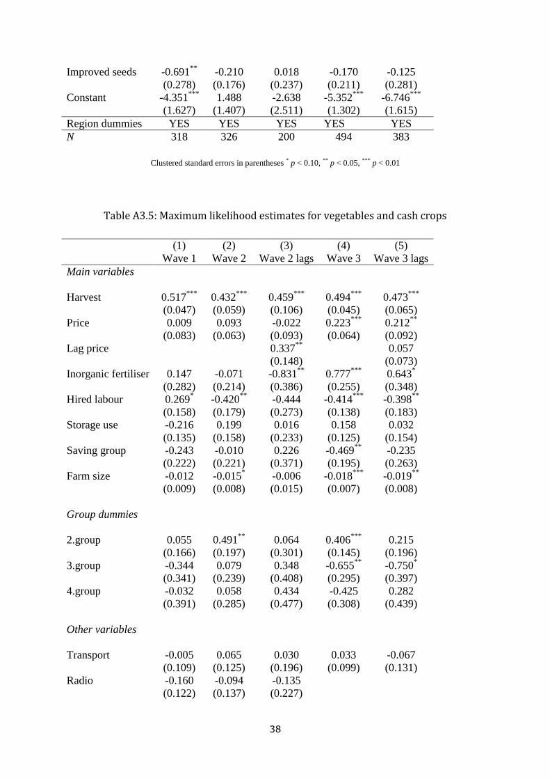
38

Improved seeds -0.691**

-0.210 0.018 -0.170 -0.125

(0.278) (0.176) (0.237) (0.211) (0.281)

Constant -4.351***

1.488 -2.638 -5.352***

-6.746***

(1.627) (1.407) (2.511) (1.302) (1.615)

Region dummies YES YES YES YES YES

N 318 326 200 494 383

Clustered standard errors in parentheses * p < 0.10, ** p < 0.05, *** p < 0.01

Table A3.5: Maximum likelihood estimates for vegetables and cash crops

(1) (2) (3) (4) (5)

Wave 1 Wave 2 Wave 2 lags Wave 3 Wave 3 lags

Main variables

Harvest 0.517***

0.432***

0.459***

0.494***

0.473***

(0.047) (0.059) (0.106) (0.045) (0.065)

Price 0.009 0.093 -0.022 0.223***

0.212**

(0.083) (0.063) (0.093) (0.064) (0.092)

Lag price 0.337**

0.057

(0.148) (0.073)

Inorganic fertiliser 0.147 -0.071 -0.831**

0.777***

0.643*

(0.282) (0.214) (0.386) (0.255) (0.348)

Hired labour 0.269* -0.420

** -0.444 -0.414

*** -0.398

**

(0.158) (0.179) (0.273) (0.138) (0.183)

Storage use -0.216 0.199 0.016 0.158 0.032

(0.135) (0.158) (0.233) (0.125) (0.154)

Saving group -0.243 -0.010 0.226 -0.469**

-0.235

(0.222) (0.221) (0.371) (0.195) (0.263)

Farm size -0.012 -0.015* -0.006 -0.018

*** -0.019

**

Group dummies

(0.009) (0.008) (0.015) (0.007) (0.008)

2.group 0.055 0.491**

0.064 0.406***

0.215

(0.166) (0.197) (0.301) (0.145) (0.196)

3.group -0.344 0.079 0.348 -0.655**

-0.750*

(0.341) (0.239) (0.408) (0.295) (0.397)

4.group -0.032 0.058 0.434 -0.425 0.282

Other variables

(0.391) (0.285) (0.477) (0.308) (0.439)

Transport -0.005 0.065 0.030 0.033 -0.067

(0.109) (0.125) (0.196) (0.099) (0.131)

Radio -0.160 -0.094 -0.135

(0.122) (0.137) (0.227)

39

Newspaper 0.033 0.269* -0.016

(0.134) (0.162) (0.246)

Head educ 0.126 -0.083 -0.375**

0.056 0.035

(0.103) (0.111) (0.187) (0.078) (0.105)

Intercrop -0.104 0.196 -0.027 0.156 0.233

(0.118) (0.145) (0.220) (0.109) (0.143)

Organic fertiliser -0.000 -0.000 -0.000 -0.000***

-0.000*

(0.000) (0.000) (0.000) (0.000) (0.000)

Distance 0.023 0.062 0.055 0.107**

0.100

(0.053) (0.055) (0.089) (0.048) (0.062)

Cooperative -0.035 -0.081 0.123 -0.032 0.052

(0.112) (0.125) (0.226) (0.099) (0.128)

Improved seeds 0.077 -0.100 -0.166 0.023 0.141

(0.127) (0.132) (0.244) (0.106) (0.138)

Lag price 0.337**

0.057

(0.148) (0.073)

Constant -2.019***

-2.764***

-3.152**

-4.063***

-4.296***

(0.700) (0.696) (1.507) (0.644) (0.907)

Region dummies YES YES YES YES YES

N 938 668 271 1111 639

Clustered standard errors in parentheses * p < 0.10, ** p < 0.05, *** p < 0.01

Table A3.6: Maximum likelihood estimates for rice and cereals crops

(1) (2) (3) (4) (5)

Wave 1 Wave 2 Wave 2 lags Wave 3 Wave 3 lags

Main variables

Harvest 0.455***

0.876***

0.974***

0.709***

0.780***

(0.083) (0.103) (0.147) (0.073) (0.088)

Price -0.085 -0.240 -0.353 -0.068 -0.024

(0.163) (0.276) (0.331) (0.155) (0.186)

Lag price 0.588* 0.134

(0.301) (0.164)

Inorganic fertiliser 0.208 0.563 0.144 -0.109 0.125

(0.408) (0.376) (0.511) (0.409) (0.432)

Hired labour 0.401 0.095 -0.043 0.119 -0.193

(0.267) (0.258) (0.364) (0.225) (0.286)

Storage use 0.291* 0.297

* -0.000 -0.036 -0.077

(0.158) (0.176) (0.235) (0.152) (0.178)

Saving group 0.203 -0.367 -1.770***

-0.200 -0.273

(0.453) (0.444) (0.440) (0.333) (0.436)

Farm size -0.032***

-0.015 -0.017 -0.019**

-0.014

Group dummies

(0.012) (0.010) (0.014) (0.009) (0.010)

40

2.group -0.367 -0.103 0.043 -0.184 0.065

(0.266) (0.265) (0.376) (0.244) (0.305)

3.group -0.140 0.234 0.792 0.706 0.671

(0.473) (0.477) (0.784) (0.517) (0.611)

4.group -0.392 0.163 -0.324 0.321 0.476

Other variables

(0.571) (0.627) (0.747) (0.525) (0.600)

Transport -0.003 0.059 0.042 -0.396***

-0.568***

(0.147) (0.173) (0.227) (0.134) (0.160)

Radio 0.210 -0.059 -0.244

(0.163) (0.164) (0.220)

Newspaper -0.084 -0.381 -0.362

(0.222) (0.257) (0.401)

Head educ 0.266* 0.263

* 0.564

*** 0.179

* 0.160

(0.144) (0.153) (0.216) (0.107) (0.124)

Intercrop 0.365**

0.215 0.221 0.208 0.278

(0.145) (0.183) (0.260) (0.150) (0.180)

Organic fertiliser 0.000 -0.000 0.000 -0.000 -0.000

(0.000) (0.000) (0.000) (0.000) (0.000)

Distance 0.028 0.053 -0.003 0.065 0.048

(0.072) (0.095) (0.123) (0.060) (0.070)

Cooperative 0.273* -0.519

*** -0.570

** -0.005 0.029

(0.148) (0.184) (0.236) (0.137) (0.162)

Improved seeds 0.119 0.169 0.044 -0.410***

-0.384**

(0.201) (0.166) (0.237) (0.140) (0.163)

Lag price 0.588* 0.134

(0.301) (0.164)

Constant -4.657***

-4.950***

-7.256***

-4.091***

-5.532***

(1.032) (1.689) (2.169) (1.110) (1.595)

Region dummies YES YES YES YES YES

N 510 473 258 631 468

Clustered standard errors in parentheses * p < 0.10, ** p < 0.05, *** p < 0.01

Table A3.7: Maximum likelihood estimates for fruit crops

(1) (2) (3) (4) (5)

Wave 1 Wave 2 Wave 2 lags Wave 3 Wave 3 lags

Main variables

Harvest 0.261***

0.438***

0.432***

0.465***

0.461***

(0.024) (0.034) (0.040) (0.026) (0.032)

Price -0.021 -0.038 -0.089 -0.003 -0.019

(0.047) (0.051) (0.072) (0.044) (0.051)

Lag price -0.001 -0.003

(0.067) (0.043)

41

Inorganic fertiliser -0.235 -0.145 -0.221 -0.242 -0.276

(0.187) (0.145) (0.177) (0.150) (0.183)

Hired labour 0.082 0.071 0.181 0.000 -0.069

(0.126) (0.130) (0.154) (0.104) (0.120)

Storage use -0.090 -0.391 -0.112 -0.313 -0.128

(0.262) (0.249) (0.287) (0.362) (0.454)

Saving group 0.092 0.046 0.276* -0.111 -0.079

(0.181) (0.128) (0.163) (0.166) (0.187)

Farm size 0.015 -0.009 -0.032**

-0.003 -0.001

Group dummies

(0.010) (0.006) (0.013) (0.003) (0.003)

2.group 0.102 -0.068 -0.200 0.036 0.090

(0.141) (0.149) (0.188) (0.121) (0.141)

3.group 0.258 -0.140 -0.107 -0.375* -0.301

(0.255) (0.181) (0.236) (0.216) (0.252)

4.group 0.259 -0.088 -0.092 0.033 -0.102

Other variables

(0.264) (0.278) (0.348) (0.240) (0.284)

Transport -0.062 0.199**

0.196* -0.201

*** -0.174

**

(0.088) (0.086) (0.116) (0.075) (0.084)

Radio -0.069 -0.006 -0.007

(0.107) (0.102) (0.129)

Newspaper -0.147 -0.328***

-0.537***

(0.106) (0.115) (0.163)

Head educ -0.082 -0.072 -0.186* -0.063 -0.099

(0.076) (0.079) (0.103) (0.059) (0.066)

Intercrop 0.134 -0.179 -0.322**

0.016 -0.051

(0.122) (0.117) (0.152) (0.110) (0.131)

Organic fertiliser -0.000 -0.000 0.000 0.000 0.000

(0.000) (0.000) (0.000) (0.000) (0.000)

Distance 0.030 -0.009 0.020 0.006 -0.012

(0.042) (0.036) (0.052) (0.036) (0.040)

Cooperative -0.034 -0.110 -0.081 -0.052 -0.021

(0.091) (0.086) (0.112) (0.074) (0.084)

Improved seeds 0.011 0.135 0.258**

0.041 0.030

(0.094) (0.096) (0.126) (0.084) (0.094)

Constant -0.680 -0.699 -0.724 -2.436**

-2.582**

(0.727) (0.810) (1.024) (1.009) (1.171)

Region dummies YES YES YES YES YES

N 1657 1620 833 2243 1576

Clustered standard errors in parentheses * p < 0.10, ** p < 0.05, *** p < 0.01