the municipal bond federal tax exemption and …
TRANSCRIPT
THE MUNICIPAL BOND FEDERAL TAX EXEMPTION AND NATIONAL CREDIT CONDITIONS
A Thesis submitted to the Faculty of the
Graduate School of Arts and Sciences of Georgetown University
in partial fulfillment of the requirements for the degree of
Master of Public Policy in Public Policy
By
Alexander J. Karjeker, B.S., B.A.
Washington, DC April, 12, 2012

ii
Copyright 2012 by Alexander J. Karjeker All Rights Reserved

iii
THE MUNICIPAL BOND FEDERAL TAX EXEMPTION AND NATIONAL CREDIT CONDITIONS
Alexander J. Karjeker, B.S., B.A.
Thesis Advisor: Jeffrey Larrimore, Ph.D.
ABSTRACT
This paper builds on existing literature in estimating the determinants of municipal bond
interest rates (yields). Much of that body of work has taken into account various factors,
including most prominently, federal income tax rates and the municipal bond interest exemption.
After the most recent financial crisis and policy response, new market data has become available
to measure the riskiness of these bonds during a major recession and liquidity crunch. Further,
current policy discussions now include the removal of the exemption. This research will examine
what effect such policy would have on municipal bond yields and additionally, whether that
effect would be the same or different in a post-financial crisis environment. The results indicate
that a change in this policy would increase yields in a statistically significant way. However,
changing policy in a post-financial crisis environment would not move yields in a perceivable
way, though the effect is statistically significant. These are important conclusions for policy
makers to consider when evaluating budgetary priorities.

iv
The research and writing of this thesis could not have been accomplished without the (large reserves of) patience and support of Dr. Jeffrey Larrimore.
Many thanks,
Alexander J. Karjeker
v
Table Of Contents
Section I: Introduction .................................................................................................................... 1
Section II: Primer on Municipal Bonds .......................................................................................... 4
Section III: Theoretical Framework and Previous Literature ......................................................... 7
Figure 1: Historical Yearly TED Spread Average.................................................................... 10 Section IV: Data Analysis............................................................................................................. 10
Figure 2: Historical Top Marginal Income Tax Rate................................................................ 11 Table 1 – Description of Variables ........................................................................................... 13 Table 2 – Summary Statistics ................................................................................................... 13
Section V: Results......................................................................................................................... 14
Table 3 – Regression Results (Prior literature) Dependent Variable: Yield Differential ......... 16 Table 4 – Continued Regression Results (Post 1986, Long Term Bonds): Dependent Variable: Yield Differential ...................................................................................................................... 20
References..................................................................................................................................... 23

1
Section I: Introduction
During the post-World War II period, state and local governments expanded their use of
municipal bonds as a means of funding for capital investments. The current market is
approximately $2.7 trillion. Considering it a compelling national interest, the United States
federal government exempted the interest payments to investors from income taxation (though
some literature questions the economic efficiency of this subsidy – Gordon and Metcalf [1991]).
The value of the tax-exemption can be quantified as the difference between the interest rates
(yields) offered on municipal bonds versus those offered on corporate bonds; the former are
lower. Since investors in municipal bonds do not have to pay taxes, the pre-tax returns are lower.
Because of its large importance in the market place and in the federal budget ($225 billion over
10 years), many economists have researched the value of this exemption and the relationship
between federal marginal income tax rates and municipal bond yields [Kidwell, Koch and Stock
(1984), Poterba (1986), and Green (1993)].
In the aftermath of the financial crisis of 2007-2008 and the political response in 2010,
the federal deficit has also come under higher scrutiny. While many argue for lower government
spending, the conversation also included increasing revenues. Inevitably, this conversation led to
a broader discussion of the tax code and its fairness. In 2011, President Obama proposed to limit
deductions and exemptions for individuals paying the top marginal income tax rate; among them
was the municipal bond interest exemption. His proposal would limit the exemption for those in
the top bracket to 28%, as opposed to their current break of 35% (or rather, he would increase the
applicable tax by 7%). As a result of this change in policy, investors in the top income brackets
would have to pay taxes on the interest payments they receive from the bonds. They would then
demand more interest from the issuing government. Banks and issuing governments recognized

2
the effect and immediately attacked this proposal as a tax hike that would raise rates and thereby
increase costs for borrowers. This paper will address this policy proposal by isolating the effect
of a decrease in taxes during a post financial crisis period characterized by decreasing liquidity
and fiscal stress. We choose a decrease in taxes as the policy equivalent of eliminating the
exemption because the group of investors that would continue to take advantage of the tax
preference would be approximately the same as if the top marginal rate was lowered.
Much of the prior research done in this area has highlighted the relationship between
municipal bonds and taxable bonds of similar risk and value. These papers find a statistically
significant positive relationship between marginal tax rates and municipal bond yields [Poterba
(1986)]. The general theory assumes that the marginal investor would purchase assets so that, on
margin, he would be indifferent between a taxable investment (such as a Treasury or corporate
bond) and a tax-exempt investment (a municipal bond) – though this model has been contested,
especially with respects to individuals designing portfolios with tax avoidance strategies in mind
[Green (1993)] or if the institution itself is a non-profit institution [Mankiw and Poterba (1996)].
Most models estimate implied marginal tax rates close to the statuary amounts for short term
bonds, but too low for long term bonds. Specifically, this earlier research has found that long
term municipal bonds have yields too high given the benefit of tax exemption (or rather, if the
only difference between taxable assets and non-taxable assets is their tax status). Determining the
remaining differences is part of the “muni bond puzzle” literature. Some economists have
attributed these differences to potential default risk [Trzcinka (1982)], additional market
uncertainty inherent in governments [Joehnk and Kidwell (1984)], market liquidity [Wang, Wu
and Zhang (2008) and Longstaff (2011)] and fixed state effects [Kidwell, Koch and Stock (1984)
and Kidwell, Koch and Stock (1984)]. However, none of these approaches completely account

3
for the discrepancy. Further, after the Tax Reform Act of 1986 changed the exemption so that
banks could not perform tax arbitrage, the market has significantly changed leading to more
individual investors in the market place and a change in determinants such as the inclusion of
systemic risk and liquidity factors. [Chalmers (1998), Chalmers (2006)].
Most relevant to the current question are the papers involving market uncertainty and
market liquidity. In the aftermath of financial crises, financial institutions are less eager to lend
and consumers are less eager to borrow, leading to slower economic growth, higher uncertainty,
and, in the case of state and local governments, lower receipts and higher expenditures. This
paper will take advantage of recent municipal bond data from after the 2008 financial crisis to
estimate the effect of changing tax policy after a financial crisis. The results suggest that industry
was correct in their assessment that eliminating the tax exemption for high income individuals
would increase yields, though not to the extent to which they believed. This study agrees with the
existing literature in the direction of that policy effect and adds to it that during periods of post
financial shock there is an additional increase in yields. Presumably one might argue that the tax
exemption was the most important factor in continued investment in municipal bonds.
The rest of the paper will proceed as follows: For those unfamiliar with municipal bonds,
Section II will offer a primer, Section III which will outlines the theoretical framework and
previous literature on municipal bond yields, Section IV will summarize the data used in this
paper, Section V will present the regression estimates and Section VI will discuss the policy
conclusions.

4
Section II: Primer on Municipal Bonds
A bond is a financial instrument by which the investor pays some amount, the principal,
to the issuing entity and in return, the entity promises to pay a percentage of that principal every
pay period for the life of the bond. At the end of that period, the entity returns the original
principal to the bond holder. The purchase price is usually referred to as “par” and the interest
payments as “coupon payments”. The pay period is generally every six months and the total life
of the bond is called its maturity length. The percentage of interest is usually referred to as
“yield”. Before the passage of the federal income tax, these bonds would (in equilibrium) pay the
same yield as private sector bonds. However, with the establishment of the modern federal
income tax, municipal bond interest escaped taxation while private sector bonds (and US
Treasuries) did not. The result of this policy arrangement is that municipal bonds offer a smaller
yield than other similar bonds.
Since the founding of the United States, state and local governments have issued bonds in
order to raise funds for various public projects. Even before the United States was founded, the
Revolutionary War was funded by state issued bonds that were later taken over by the federal
government. State and local governments have used these funds to pay for needs as diverse as
infrastructure projects like roads, canals, and dams or to finance the construction of schools,
hospitals and ports (among other projects).
Types of Bonds
In the past, most localities backed their bonds by the “full faith and credit” of the
government. This is the same as the “full faith and credit” of the United States government with
respect to its Treasury bonds. This meant that the coupons (interest payments) were to be paid

5
out of the government’s general treasury account. In the past, and continuing today, most state
and local governments raise revenues from property taxes, or in some instances, sales taxes.
Consequently, most jurisdictions have limits on the amount of debt that can be incurred by state
and local government officials and generally require public support at an election prior to any
issuance. These bonds are called general obligation (GO) bonds.
Beginning in the 20th century, governments realized that they could specifically designate
particular revenue streams to pay their outstanding coupons. For example, governments may
decide to build an airport and charge airlines a fee for use of the airport. The transit agency
would pay the coupons from the fees gathered. Courts further ruled that voters do not have to be
consulted on these bonds. These bonds are called revenue bonds and are generally considered
riskier than GO bonds.
Together, GO bonds and revenue bonds comprise approximately 85% of the historical
market. There are other types of tax-exempt obligations that state and local governments can
issue, but they are generally limited in their scope and market share.
Insurance
Through the history of this market, state and local governments have almost never
defaulted on their obligations. The nature of governments (“infinitely lived”) and the lack of
assets available to be seized during a default poses an additional unique risk that is different from
what might be encountered by an investor vis-à-vis a corporation (See Robbins [1984]). One way
governments have tried to mitigate this unique problem (and pay lower yields) is to institute
balanced budget requirements to show fiscal strength. Beginning in the 1970s, with the New
York City financial crisis, investors began to look at the financial statements of state and local

6
authorities more closely before purchasing their bonds. In order to continue to maintain high
credit ratings, issuing governments would purchase insurance for their bonds. The insuring entity
agrees to pay investors in the event of a default by the issuing government in exchange for a one-
time premium. These supplemental packages soon became standard and would be very important
in affecting yields and credit ratings. Credit ratings on bonds were conducted by the three
national credit rating agencies, Standard and Poor’s, Moody’s, and Fitch. Their scales are the
same as for private sector debt. In the historical market more than 80% of bonds received long
term ratings of at least AA- by Standard and Poor’s.
Public Finance Impact
Since interest payments are excluded from taxable income, most bonds are purchased by
households and corporations, generally in high marginal tax brackets, in order to reduce their
effective tax liability. Prior to the Tax Reform Act of 1986, these bonds were mostly purchased
by corporations (like banks) that could arbitrage their interest; they used deposits to purchase
municipal bonds that would pay a relatively higher interest rate in order to pay their depositors
and still earn a profit (See Feenberg and Poterba [1992]). The Reform Act ended this practice
and the distribution has now shifted so that currently 2/3 of the benefits accrue to households and
1/3 to corporations (OMB [2009]). The Office of Management and Budget has estimated that the
cost of this subsidy to be $30 billion (in FY 2010) and $230 billion (in FY 2012-2016). States
also may tax-exempt their own bonds for taxpayers in their jurisdiction. This tends to concentrate
many state and local bonds in the hands of local investors as opposed to larger, national
investors.

7
Section III: Theoretical Framework and Previous Literature
In capital markets, investors seek to maximize their post-tax asset returns. On margin, an
investor, for assets of similar maturity length and credit risk, will equalize the gains from taxable
investments as non-taxable investments. Specifically, the relationship between municipal and
corporate bond yields and tax rates is:
tm yty )1( −= (1)
where ym is the yield on municipal bonds, yt is the yield on taxable bonds, and t is the marginal
tax rate. What this means is that if a corporate bond yield is 15% and the effective tax rate is
50%, then the after-tax return is 7.5%. Any municipal bonds of equal risk and maturity length
should yield 7.5% under this theoretical relationship. Another way of thinking about it is that
investors pay for the tax preference – the higher the tax rate (and more valuable the preference),
the less government pays for the capital. Expanding and rewriting this equation in terms of the
implied marginal tax rate we have:
t
y
yy
t
tm −=−
(2)
The left hand term is the percentage difference between taxable bonds and municipal bonds
relative to taxable bonds. While the negative coefficient on the marginal income tax rate seems
unusual, it will become intuitively useful in thinking about the effect on municipal bond yields
(i.e. the larger the negative value, the more municipal bonds are being offered at a discount
compared to taxable assets).

8
As previously mentioned, previous research has found that the relationship described in
equation two overstates the relationship between yield spreads and marginal income tax rates.
One explanation is that many individuals do not pay the statutory marginal tax rates; they often
pay much lower rates because of deductions and exemptions (like municipal bond interest) that
lower their total taxable income. Despite the distinction between the statutory and effective rates,
we know that a change in the overall rates will still lead to reductions in the statutory rates, all
else equal and so we use the statutory rates here [as do others in the literature – e.g. Poterba
(1986)].
Other factors that have been shown to effect yields include its maturity length, the size of
the bond offering [Hastie (1972)], whether or not it is a general obligation or revenue bond or
other [Heins (1962)], credit ratings [Rubinfeld (1973), Tanner (1975), and Capeci (1991)],
whether or not it has insurance [Kidwell, Sorenson and Wachowicz (1987)], state fixed effects
[Kidwell, Koch and Stock (1984) and Kidwell, Koch and Stock (1984)]], and the equities
market [Mankiw and Poterba (1986)]. In particular, we would expect that shorter maturity length
bonds, general obligation bonds, and those offering insurance or maintaining better credit ratings
will have lower yields. Including state fixed effects will account for the fiscal responsibility rules
established by state governments and the different tax treatments that states have for their own
bonds. These previous papers use ordinary least squares regressions, and generally assume a
linear relationship among the factors. This paper’s framework will continue in that tradition.
Further, the model will incorporate growth in gross domestic product as an additional control.
This paper’s contribution to the literature will be to incorporate a measure of aggregate
illiquidity and financial shock. During the financial crisis, both economists and non-economists
turned to the TED spread as a measure of liquidity in the financial system. The TED spread is the

9
difference between the three month LIBOR (London Interbank Offered Rate) and the three
month Treasury rate. (See Figure 1 Below) Intuitively, as LIBOR increases past Treasuries,
banks are responding to outside shocks and uncertainty that make them unlikely to allow credit
to other financial institutions – ones that are likely responding to the same outside shocks. In the
most recent financial crisis, this was the explosion of the mortgage housing bubble. This is the
spike in 2008. Otherwise, in general, TED spread values are quite low and describe a fairly
stable financial system. In addition to including this term as a linear determinant of municipal
bond yields, the regression model will also include an interaction term that will focus on the
marginal effect of a change in policy, given particular credit conditions. The equation is as
follows:
εββββ +Β++++= −
−
33210 * XTtTty
yy
t
tm (3)
where ym, yt and t are as before, T represents the TED spread and X contains the controls
previously discussed. In this model, we will use the coupon rate at issuance for ym and the
associated term Treasury bond for yt.

10
Figure 1: Historical Yearly TED Spread Average
TED Spread Yearly Averages
00.20.40.60.8
11.21.41.61.8
19841986
1988
1990
199219
9419
9619
9820
0020
0220
0420
0620
0820
10
Year
Inte
res
t R
ate
Source: Author’s calculation using Bloomberg Financial Database
Section IV: Data Analysis
Data Sources
The majority of the data was obtained from Bloomberg’s Municipal Bond Database.
Bloomberg keeps a database of all bond issues starting from the early 1980s and includes coupon
amounts, bond sale (par) amounts, the total amount borrowed as part of the bond deal, type of
bonds (general obligation, revenue or other), the type of insurance on the bond (or none), the
date of first payment on the coupons and maturity date, and the state from which the bond was
issued. The dates are important in determining the full maturity length of the bond. These bonds
were all issued between 1984 and 2010. Bloomberg was also the source for obtaining a daily
historical index of the TED Spread, and a daily history of yields on Treasury bonds for various
maturity lengths. The historical top marginal tax rate was obtained from the Tax Policy Center at
11
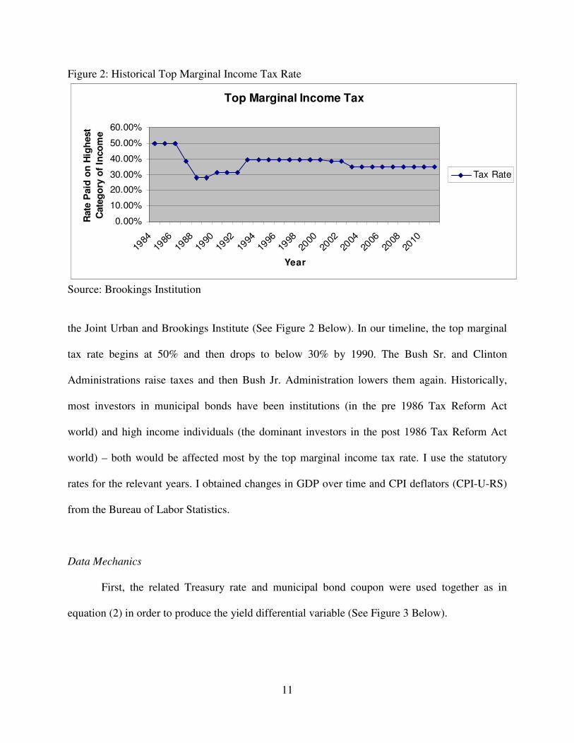
Figure 2: Historical Top Marginal Income Tax Rate
Top Marginal Income Tax
0.00%
10.00%
20.00%
30.00%
40.00%
50.00%
60.00%
1984
1986
1988
1990
1992
1994
1996
1998
2000
2002
2004
2006
2008
2010
Year
Rate
Paid
on
Hig
hest
Cate
go
ry o
f In
co
me
Tax Rate
Source: Brookings Institution
the Joint Urban and Brookings Institute (See Figure 2 Below). In our timeline, the top marginal
tax rate begins at 50% and then drops to below 30% by 1990. The Bush Sr. and Clinton
Administrations raise taxes and then Bush Jr. Administration lowers them again. Historically,
most investors in municipal bonds have been institutions (in the pre 1986 Tax Reform Act
world) and high income individuals (the dominant investors in the post 1986 Tax Reform Act
world) – both would be affected most by the top marginal income tax rate. I use the statutory
rates for the relevant years. I obtained changes in GDP over time and CPI deflators (CPI-U-RS)
from the Bureau of Labor Statistics.
Data Mechanics
First, the related Treasury rate and municipal bond coupon were used together as in
equation (2) in order to produce the yield differential variable (See Figure 3 Below).

12
Figure 3 – Average Yield Differential Over Time
Average Yield Differential Over Time (1987-2010)
-0.4
-0.2
0
0.2
0.4
0.6
0.8
1987
1989
1991
1993
1995
1997
1999
2001
2003
2005
2007
2009
Year
Perc
en
tag
e D
iffe
ren
ce
Betw
een
Mu
nic
ipal
Yie
lds
an
d T
reasu
ry R
ate
s
Source: Author’s calculation using Bloomberg Municipal Bond Database
The difference between the date of first coupon payment and the maturity date was used
to calculate each bond’s appropriate maturity length. Using both the date of issuance and the
maturity length, these bonds were matched to the relevant Treasury yield. For most large
municipal debt offerings, more than one bond is issued representing part of the total deal size.
Both the deal size associated with the bond and the bond’s actual value was deflated using CPI
data (with 2010 base year). These values’ logarithms were used in the final estimation in order to
obtain the non-linear relationship between the deal size and additional interest rate cost – an
additional $1 of debt does not have the same effect on yields as an additional $1 of debt when it
is raised from nothing as when it is raised from $100 (See Hastie [1972], Kidwell, Koch and
Stock [1984], and Joehnk and Kidwell [1984]). Indicator variables were used for the type of
bond (with general obligation bonds as the excluded case) and fifty indicator variables were
created account for state effects. Indicator variables were used to for the different Standard and
Poor’s credit rankings. Tables 1 and 2 contain descriptive and summary data.
13
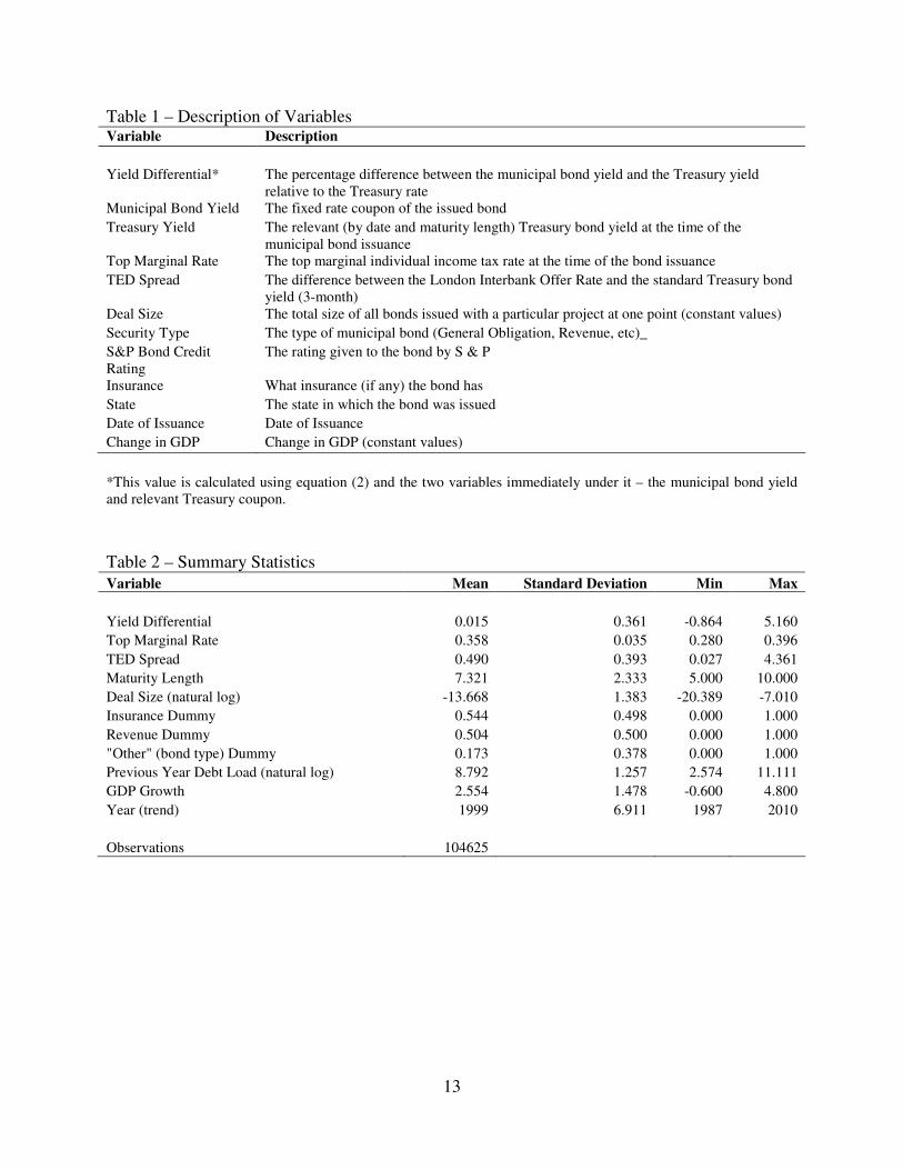
Table 1 – Description of Variables Variable Description
Yield Differential* The percentage difference between the municipal bond yield and the Treasury yield relative to the Treasury rate
Municipal Bond Yield The fixed rate coupon of the issued bond
Treasury Yield The relevant (by date and maturity length) Treasury bond yield at the time of the municipal bond issuance
Top Marginal Rate The top marginal individual income tax rate at the time of the bond issuance
TED Spread The difference between the London Interbank Offer Rate and the standard Treasury bond yield (3-month)
Deal Size The total size of all bonds issued with a particular project at one point (constant values)
Security Type The type of municipal bond (General Obligation, Revenue, etc)_
S&P Bond Credit Rating
The rating given to the bond by S & P
Insurance What insurance (if any) the bond has
State The state in which the bond was issued
Date of Issuance Date of Issuance
Change in GDP Change in GDP (constant values)
*This value is calculated using equation (2) and the two variables immediately under it – the municipal bond yield and relevant Treasury coupon.
Table 2 – Summary Statistics Variable Mean Standard Deviation Min Max
Yield Differential 0.015 0.361 -0.864 5.160
Top Marginal Rate 0.358 0.035 0.280 0.396
TED Spread 0.490 0.393 0.027 4.361
Maturity Length 7.321 2.333 5.000 10.000
Deal Size (natural log) -13.668 1.383 -20.389 -7.010
Insurance Dummy 0.544 0.498 0.000 1.000
Revenue Dummy 0.504 0.500 0.000 1.000
"Other" (bond type) Dummy 0.173 0.378 0.000 1.000
Previous Year Debt Load (natural log) 8.792 1.257 2.574 11.111
GDP Growth 2.554 1.478 -0.600 4.800
Year (trend) 1999 6.911 1987 2010
Observations 104625

14
Section V: Results
In order to appropriately discern the effect of a decrease in taxes on municipal bond
yields, the regression models were confined to those long term issuances (maturity length greater
than five years) issued after 1986. Previous literature on the determinants of municipal bond
yields have found the relationship described in (1) in short maturity length bonds, but not long
maturity length bonds. This is possibly because of the different risk associated with tax changes
over the longer maturity length bonds (Jordan and Pettway [1985]). The discrepancy between
what the model would imply and the data is known as the “muni bond puzzle” [Longstaff
(2011)]. Since long term bonds are the focus of much of the earlier research, they also are the
focus here. Bonds are limited to those issued after 1986 since they are subject to the new
provisions in the Tax Reform Act of 1986 and, unlike those issued prior to 1986, are primarily
owned by individuals as opposed to corporations (Feenberg and Poterba [1991]). The model
results are shown in Tables 3 and 4 below.
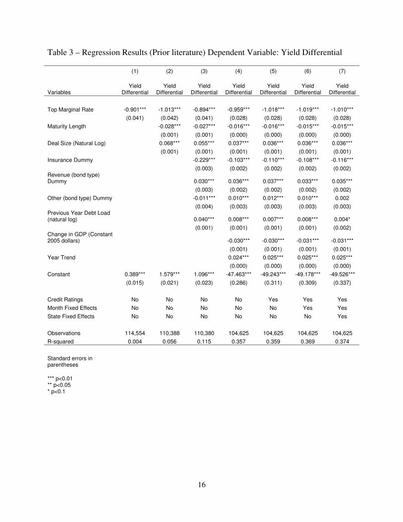
Table 3 focuses on the factors that previous research has found to be important in
determining municipal bond yields. The coefficient on the top marginal rate is significant and
negative. Per equation 2, we would expect the coefficient to be -1. In Column 1, using a simple
regression, the coefficient is not quite what the theory would expect. The 0.1 difference is much
smaller than what the previous literature suggests though it does follow the same direction. After
controlling for other factors, the marginal tax rate coefficient does not differ by more than 0.11
from -1.
In Column 2 of Table 3, we see that the coefficient is approximately -1. At this point, the
benefit of tax-exempt income is incorporated into the yield so that it is lower than its equivalent
taxable bond. This model finds that the expected gap (“muni bond puzzle”) is not present in the

15
data. Previous research had found that the benefit was not fully factored in by lower yields. One
possible explanation is that the data looks at long maturity length bond issues over twenty years
as opposed to the shorter time frames used in previous papers. The coefficient is important in
that the financial markets are able to value and trade the municipal bond tax exemption as part of
the total bond yield. The other important factor is that government tax policies will affect
municipal bond yields. These connections allow for the proposed tax changes to mean anything
to the financial market.
Column 2 of Table 3 incorporates maturity length and the size of the total bond deal. The
coefficient on the total bond deal size is intuitive – the larger the project, the larger the loans and
the higher the yield. Maturity length, on the other hand, may appear counterintuitive – the longer
a bond is active, the more risk the issuer has of default or tax laws to change. Based on this
theory, increases in maturity length will increase bond yields. However, the reader should
remember that the dependent variable is the yield differential with respect to Treasury bonds, not
simply the municipal bond yield. So if Treasury bond yields rise at a faster rate than municipal
bonds (which upon data inspection not included in this paper suggest) then the rate will be
negative. Thus, this seemingly counterintuitive result is more logical when placed in the context
of the specification of the dependent variable.
Column 3 adds the insurance and bond type dummies and lagged state debt load. These
coefficients values are generally consistent with those in the literature [Heins (1962), Kidwell
Koch (1982)], both in sign and magnitude. General Obligation bonds (the excluded set) are the
cheapest, followed by revenue bonds (Heins [1962]). Insurance drops the price of bonds
(Robbins [1984]). Since all state agencies and local governments get their authority from the
16
Table 3 – Regression Results (Prior literature) Dependent Variable: Yield Differential
(1) (2) (3) (4) (5) (6) (7)
Variables Yield
Differential Yield
Differential Yield
Differential Yield
Differential Yield
Differential Yield
Differential Yield
Differential
Top Marginal Rate -0.901*** -1.013*** -0.894*** -0.959*** -1.018*** -1.019*** -1.010***
(0.041) (0.042) (0.041) (0.028) (0.028) (0.028) (0.028)
Maturity Length -0.028*** -0.027*** -0.016*** -0.016*** -0.015*** -0.015***
(0.001) (0.001) (0.000) (0.000) (0.000) (0.000)
Deal Size (Natural Log) 0.068*** 0.055*** 0.037*** 0.036*** 0.036*** 0.036***
(0.001) (0.001) (0.001) (0.001) (0.001) (0.001)
Insurance Dummy -0.229*** -0.103*** -0.110*** -0.108*** -0.116***
(0.003) (0.002) (0.002) (0.002) (0.002) Revenue (bond type) Dummy 0.030*** 0.036*** 0.037*** 0.033*** 0.035***
(0.003) (0.002) (0.002) (0.002) (0.002)
Other (bond type) Dummy -0.011*** 0.010*** 0.012*** 0.010*** 0.002
(0.004) (0.003) (0.003) (0.003) (0.003) Previous Year Debt Load (natural log) 0.040*** 0.008*** 0.007*** 0.008*** 0.004*
(0.001) (0.001) (0.001) (0.001) (0.002) Change in GDP (Constant 2005 dollars) -0.030*** -0.030*** -0.031*** -0.031***
(0.001) (0.001) (0.001) (0.001)
Year Trend 0.024*** 0.025*** 0.025*** 0.025***
(0.000) (0.000) (0.000) (0.000)
Constant 0.389*** 1.579*** 1.096*** -47.463*** -49.243*** -49.178*** -49.526***
(0.015) (0.021) (0.023) (0.286) (0.311) (0.309) (0.337)
Credit Ratings No No No No Yes Yes Yes
Month Fixed Effects No No No No No Yes Yes
State Fixed Effects No No No No No No Yes
Observations 114,554 110,388 110,380 104,625 104,625 104,625 104,625
R-squared 0.004 0.056 0.115 0.357 0.359 0.369 0.374
Standard errors in parentheses
*** p<0.01 ** p<0.05 * p<0.1

17
State government, this model used the total debt load of a state in the past year to approximate
the aggregate risk based on outstanding issuance. The coefficient is positive showing that an
increase in previous borrowing adds to the cost of current and prospective borrowing. Column 4
of Table 3 incorporates the macroeconomic variables. As the economy grows, businesses
demand more investment and so municipal bond issuers must increase yields to compete with the
private sector. However, the Federal Reserve raises interest rates on its bonds at a faster rate (to
contact the money supply) and consequently, the coefficient on the yield differential is negative.
Column 4 also includes a year trend. Columns 6 and 7 of Table 3 add controls for the bond’s
credit rating, state fixed effects and month of issuance effects. The reader may note that the
credit rating dummies do not provide much additional information to the model (the R-squared
does not move as much). This is due to the small amount of variation in the credit rating
dummies. No observations in this subset had bond ratings below BBB–. The variables in Column
7 agree with the existing literature in effect and significance with the exception of the top
marginal income tax rate. That effect agrees with the theoretical model, but not the prior
empirical literature.
The previous literature has not focused on the potential effect of a financial crisis on bond
yields and the effect it may have on investor appetite. Table 4 incorporates variables that
describe the broader financial state of the economy, not previously discussed in the literature.
Columns 1 and 2 incorporate the TED spread as a measure of aggregate market illiquidity and
the post-financial shock reality. Column 2 adds an interaction term between the top marginal rate
and the measure of illiquidity in the financial system. In column 2, the final model incorporates
the interaction between the top marginal rate and the TED spread. In this model, which is my
preferred specification, the coefficient on the top marginal rate is -0.785 and is statistically

18
significant. The model implies that a 1 point increase in the top marginal rate would decrease the
bond differential by .00785. Since the bond differential is the difference between the municipal
bond yield and the Treasury bond yield divided by the Treasury bond yield, we can say that the
yield differential would decrease by 0.785%, or a little more than three-quarters of a basis points
for every percentage in Treasury yield. The previous statement in italics is to say that for a 1%
yield on a Treasury bond, the yield differential decreases by three-quarters of a basis point.
Similarly, for a Treasury bond with a 4% yield, the effect would lower municipal bond yields by
three basis points. In 1993, the Clinton Administration raised top marginal income tax rates by
8.6%. At that time, the average long term municipal bond yield was 5.88% and the average long
term Treasury bond yield was 6.16% - a difference of 28 basis points. The models predicts that
the difference will drop by 4 basis points. In 1993, the average long term Treasury bond yield
was 5.31% and the average long term municipal bond yield was 5.09% - a difference of 24 basis
points, or 4 basis points less than the 1992 values.
The coefficient on the TED spread is positive (0.152) and also statistically significant.
During periods of large strain on the financial system, central bankers lower interest rates (on
Treasury bonds) in order to provide liquidity and avoid systemic collapses. However investors
(after adjusting for risk), still find that long term bonds are not safe enough and increase their
demands for security (trading in favor of higher compensation, i.e. higher yields relative to
Treasury bonds). For every 100 basis point increase in the TED spread, there is a 15.2% increase
or 15 basis points for every percentage in Treasury yield.
The effects of changes to the top marginal rate and the TED spread are also significant
when interacted, though their actual magnitude is small. The interaction coefficient is negative (-
.003). At a 35% tax rate, for every 100 basis point increase, the interaction implies a one-tenth of

19
a basis point additional decrease for every percentage in Treasury yield. The interaction does not
significantly change the effect of the TED spread in any given tax environment. For example,
with a 39.6 percent marginal tax rate, which is the highest observed during this period, when
including the interaction effect the impact of a 100 basis point increase in the TED spread is a 15
percent change in the yield differential. This compares to a 15.1 percent change in the yield
differential from a 100 basis point increase in the TED spread with a 28 percent marginal tax
rate, which was the lowest observed during this period.
We now turn to the marginal effect of the highest marginal income tax interaction under
different financial stress environments. Under normal circumstances (TED spread of 0.25 – the
average in 1995), for every 1% increase in the top marginal tax rate, the yield differential drops
by .00075 or an additional seven percent of one basis point per percentage in Treasury yield due
to the interaction – an almost imperceptible change in the yield differential. During periods of
high financial stress (on average, the TED spread was 3.5 in October 2008), every 1% increase in
the top marginal tax rate drops the yield differential by .00001 per percentage in Treasury yield
– or again a very non-perceivable change in yields. In other words, tax policy simply isn’t that
important during true liquidity crises – yields may move, but not by any significant amount.

20
Table 4 – Continued Regression Results (Post 1986, Long Term Bonds): Dependent Variable:
Yield Differential
(1) (2)
Variables Yield Differential Yield Differential
Top Marginal Rate -0.957*** -0.785***
(0.028) (0.053)
TED Spread 0.049*** 0.152***
(0.002) (0.027)
Interaction between the TED Spread and Top Marginal Rate -0.003***
(0.001)
Maturity Length -0.015*** -0.015***
(0.000) (0.000)
Deal Size (Natural Log) 0.036*** 0.036***
(0.001) (0.001)
Insurance Dummy -0.113*** -0.113***
(0.002) (0.002)
Revenue (bond type) Dummy 0.034*** 0.035***
(0.002) (0.002)
Other (bond type) Dummy 0.001 0.001
(0.003) (0.003)
Previous Year Debt Load (natural log) 0.005** 0.006**
(0.002) (0.002)
Change in GDP (Constant 2005 dollars) -0.030*** -0.030***
(0.001) (0.001)
Year Trend 0.026*** 0.026***
(0.000) (0.000)
Constant -50.277*** -50.409***
(0.338) (0.340)
Credit Ratings Yes Yes
Fixed Month Effects Yes Yes
Fixed State Effects Yes Yes
Observations 104,625 104,625
R-squared 0.377 0.377
Standard errors in parentheses
*** p<0.01, ** p<0.05, * p<0.1

21
Section VI: Conclusion and Policy Implications
Concurring with the existing research, this paper finds evidence that the tax policy alone
does not explain the difference between yields on taxable and non-taxable assets. The results also
confirm many of the other factors that affect the differing yields. Where this paper differs is in
analyzing the effects of a financial crisis on the tradeoffs that investors will make between
security and compensation. During periods of normalcy, this paper affirms that investors are very
salient to tax changes and respond strongly to any changes. And in crisis, these preferences are
even further cemented as the tax preference becomes a larger factor in the value of the bond,
though the additional focus is not very large.
Looking at Tables 5 and 6, President Obama’s proposal to limit the tax exemption for
municipal bonds would have raised yields required by municipal bond issuers to raise capital
during a financial crisis environment, but only by an additional very small amount. The
heightened risks would not have offset any concern about taxes or the federal government. One
reason why this might be the case is that historically the default rate on municipalities has been
very small. Further, as evidenced in the most recent case, bond holders may believe that the
federal government, which has lowered rates on Treasury bonds and received an influx of
capital, will use that capital to assist state budgets and help them meet their obligations. At the
same time, state and local governments could also be highly sensitive to the idea of defaulting,
especially given the dearth of defaults and the future capital costs that they would incur when
coming back to the market for funds. Another factor involved is that raising local taxes or
defaulting on bonds generally affects the same population – the highest income and wealthiest
individuals in the community (especially in areas where additional tax breaks are given for local
residents to own their community’s bonds). It is conceivable that during financial crises, these
22
individuals understand that they will take loses in one form or another – higher tax rates or bond
defaults – and are therefore unmoved by the financial crises in general.
Policy makers should be aware of these effects because they help determine the
interaction between government and the financial markets. The top marginal tax rate does help
determine the overall municipal bond yield and changing it, or other relevant tax options, does
have an important effect. Financial markets, and indeed all markets, are complex systems that
can have unusual reactions to outside shocks, such as a financial crisis. These events should be
analyzed to determine if there are any “out of the box” or unexpected phenomenon. This paper
shows that the most recent financial crisis did not have a major unexpected reaction on the effect
of top marginal tax rates on municipal bond yields and that policy makers should continue with
their understanding of the interaction between market forces and tax policy.
23
References
Capeci, John. "Credit Risk, Credit Ratings, and Municipal Bond Yields: A Panel Study."
National Tax Journal 45 (1991): 41-56. Web. Chalmers, John M. R. "Default Risk Cannot Explain the Muni Puzzle: Evidence from Municipal
Bonds That Are Secured by U.S. Treasury Obligations." The Review of Financial Studies 11.2 (1998): 281-308. Web.
Chalmers, John M. R. "Systematic Risk and the Muni Puzzle." National Tax Journal 59.4
(2006): 838-48. Web. Erickson, Merle, Austan Goolsbee, and Edward Maydew. "How Prevalent Is Tax Arbitrage?
Evidence from the Market for Municipal Bonds." National Bureau of Economics. Web. <http://www.nber.org/papers/w9105>.
Feenberg, Daniel R., and James M. Poterba. "Which Households Own Municipal Bonds?
Evidence From Tax Returns." National Tax Journal 44.4 (1992): 93-103. The National
Bureau of Economic Research. NBER. Web. <http://www.nber.org/papers/w3900>. Gordon, Roger H., and Gilbert E. Metcalf. "Do Tax-Exempt Bonds Really Subsidize Municipal
Capital?" National Bureau of Economics (1991). The National Bureau of Economic
Research. Web. <http://www.nber.org/papers/w3835>. Green, Richard C. "A Simple Model of the Taxable and Tax-Exempt Curves." The Review of
Financial Studies 6.2 (1993): 233-64. Web. Hastie, K. Larry. "Determinants of Municipal Bond Yields." The Journal of Financial and
Quantitative Analysis 7.3 (1972): 1729-748. JSTOR. JSTOR. Web. <http://www.jstor.org/stable/2329798>.
Heins, A. James. "The Interest Rate Differential Between Revenue Bonds and General
Obligations: A Regression Model." National Tax Journal 15.4 (1962): 399-406. ProQuest. ProQuest. Web.
Joehnk, Michael D., and David S. Kidwell. "The Impact of Market Uncertainty on Municipal
Bond Underwriter Spread." Financial Management 13.1 (1984): 37-44. JSTOR. JSTOR. Web. <http://www.jstor.org/stable/3665122>.
Jordan, Bradford D., and Richard H. Pettway. "The Pricing of Short-Term Debt and the Miller
Hypothesis: A Note." The Journal of Finance 40.2 (1985): 589-94. Wiley-Blackwell. Web.
Kidwell, David S., Eric H. Sorenson, and John M. Wachowicz, Jr. "Estimating the Signaling
Benefits of Debt Insurance: The Case of Municipal Bonds." The Journal of Financial and
24
Quantitative Analysis 22.3 (1987): 299-313. JSTOR. JSTOR. Web. <http://www.jstor.org/stable/2330965.>.
Kidwell, David S., Timothy W. Koch, and Duane R. Stock. "The Impact of State Income Taxes
on Municipal Borrowing Costs." National Tax Journal (1984). Web. Longstaff, Francis A. "Municipal Debt and Marginal Tax Rates: Is There a Tax Premium in
Asset Prices?" The Journal of Finance 66.3 (2011). Web. Mankiw, N. Gregory, and James M. Poterba. "Stock Market Yields and the Pricing of Municipal
Bonds." NBER. The National Bureau of Economic Research. Web. 23 Mar. 2012. <http://www.nber.org/papers/w5607>.
Office of Management and Budget. "Tax Expenditures Spreadsheet." The White House. The
White House, 2009. Web. <http://www.whitehouse.gov/sites/default/files/omb/budget/fy2013/assets/teb2013.xls>.
Poterba, James M. "Explaining the Yield Spread between Taxable and Tax-exempt Bonds : The
Role of Expected Tax Policy." Studies in State and Local Public Finance. Chicago: University of Chicago, 1986. 5-52. Web. <http://www.nber.org/chapters/c8896>.
Robbins, Edward Henry. "Pricing Municipal Debt." The Journal of Financial and Quantitative
Analysis 19.4 (1984): 467-83. Web. Rubinfeld, Daniel. "Credit Ratings and the Market for General Obligation Municipal Bonds."
National Tax Journal 26.1 (1973). Web. Tanner, J. Ernest. "The Determinants of Interest Cost on New Municipal Bonds: A
Reevaluation." The Journal of Business 48.1 (1975): 74-80. JSTOR. JSTOR. Web. <http://www.jstor.org/stable/2352410 .>.
Trzcinka, Charles. "The Pricing of Tax-Exempt Bonds and the Miller Hypothesis." The Journal
of Finance 37.4 (1982): 907-23. JSTOR. JSTOR. Web. <http://www.jstor.org/stable/2327757 .>.
Wang, Junbo, Chunchi Wu, and Frank X. Zhang. "Liquidity, Default, Taxes, and Yields on
Municipal Bonds." Journal of Banking and Finance 32 (2008): 1139-149. ScienceDirect. ScienceDirect. Web.