the modelling of reinsurance credit risk (2) 031007 · the modelling of reinsurance credit risk 2-5...

1

34th Annual GIRO Convention

The Modelling of Reinsurance Credit Risk

2-5 October 2007Celtic Manor, Newport, Wales

R A ShawGuy Carpenter

Topics

� Reinsurance Credit Risk

� The Loss Process

� Diversification and Correlation

� Rating Agency Studies

� Modelling Reinsurance Credit Risk Loss

� Numerical Examples

� Modelling Issues

2

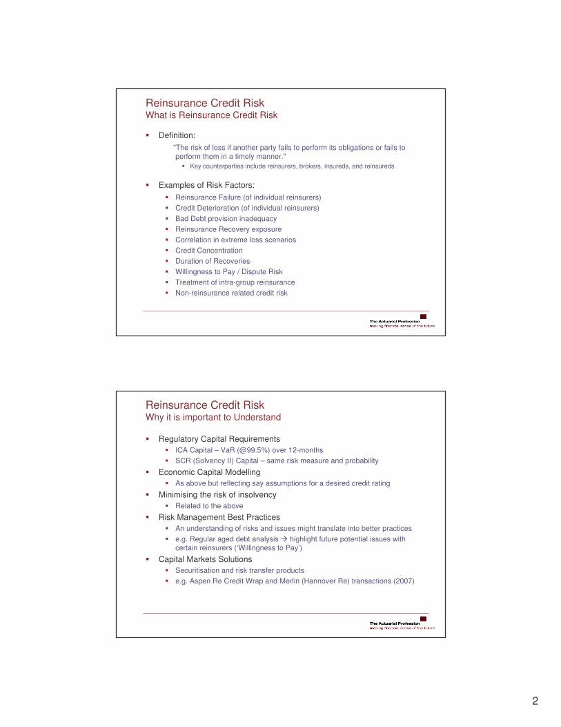
Reinsurance Credit RiskWhat is Reinsurance Credit Risk

� Definition:"The risk of loss if another party fails to perform its obligations or fails to perform them in a timely manner."

� Key counterparties include reinsurers, brokers, insureds, and reinsureds

� Examples of Risk Factors:� Reinsurance Failure (of individual reinsurers) � Credit Deterioration (of individual reinsurers) � Bad Debt provision inadequacy � Reinsurance Recovery exposure� Correlation in extreme loss scenarios� Credit Concentration� Duration of Recoveries� Willingness to Pay / Dispute Risk � Treatment of intra-group reinsurance� Non-reinsurance related credit risk

Reinsurance Credit RiskWhy it is important to Understand

� Regulatory Capital Requirements� ICA Capital – VaR (@99.5%) over 12-months� SCR (Solvency II) Capital – same risk measure and probability

� Economic Capital Modelling� As above but reflecting say assumptions for a desired credit rating

� Minimising the risk of insolvency� Related to the above

� Risk Management Best Practices� An understanding of risks and issues might translate into better practices� e.g. Regular aged debt analysis � highlight future potential issues with

certain reinsurers (‘Willingness to Pay’)

� Capital Markets Solutions� Securitisation and risk transfer products� e.g. Aspen Re Credit Wrap and Merlin (Hannover Re) transactions (2007)

3

Reinsurance Credit RiskWhy it is important to Understand

� Reinsurance Purchasing decision making:� Can play a part in determining the optimal reinsurance structure� Modification in the NPV of the net loss and underwriting profit distributions

� Impact greatest at the highest loss percentiles

� More relevant for longer-tail lines:� Reserves take a few years to run-off (albeit declining exposure)� Not a big number in year 1 – highly rated companies � Yesterday’s ‘A’ rated companies suffer downgrades over time

� In addition at the extreme loss percentiles� Very Large Property Cat Loss � increase in reinsurance default rates

� Reinsurance Panel Evaluation:� Given a new reinsurance program how should it be placed

� 100% with one reinsurer� Smaller shares with others (Rating ?)

� Benefits of Diversification � Credit Risk� Similar considerations when making reinsurance purchasing decisions

Reinsurance Credit RiskManaging Reinsurance Counterparty Risk

� Risk Management Practices of ways to manage the Risk :� Greater risk retention – i.e. reinsure less� Establishment of an established credit risk committee, which reviews the

credit ratings of reinsurers, brokers and coverholders on a regular basis. � Focus on reinsurer’s ‘Willingness to Pay’ and not just credit rating� The instigation of formal procedures for reinsurance purchasing � Having a formal policy and procedures for the evaluation, usage and

monitoring of new and existing reinsurance security. � As above but the process to embrace new and existing brokers. � Regular review of concentrations within individual custodians, group

companies, or geographic locations. � The monitoring and reporting of historical accumulated exposures� Regular aged debt analysis and reporting � Regular internal audit reviews of controls over third party credit risk � Downgrade clauses in reinsurance treaties.

4

Topics








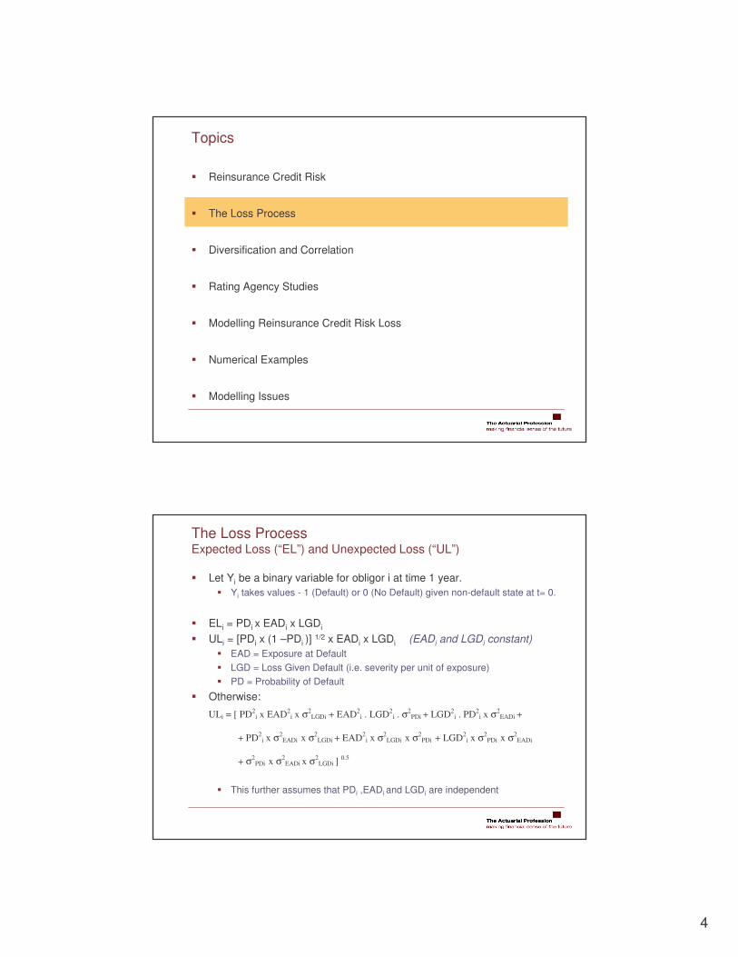
The Loss ProcessExpected Loss (“EL”) and Unexpected Loss (“UL”)

� Let Yi be a binary variable for obligor i at time 1 year. � Yi takes values - 1 (Default) or 0 (No Default) given non-default state at t= 0.

� ELi = PDi x EADi x LGDi

� ULi = [PDi x (1 –PDi )] 1/2 x EADi x LGDi (EADi and LGDi constant)� EAD = Exposure at Default� LGD = Loss Given Default (i.e. severity per unit of exposure)� PD = Probability of Default

� Otherwise:

� This further assumes that PDi ,EADi and LGDi are independent

ULi = [ PD2i x EAD2

i x σ2LGDi + EAD2

i . LGD2i . σ2

PDi + LGD2i . PD2

i x σ2EADi +

+ PD2i x σ2

EADi x σ2LGDi + EAD2

i x σ2LGDi x σ2

PDi + LGD2i x σ2

PDi x σ2EADi

+ σ2PDi x σ2

EADi x σ2LGDi ] 0.5

5

The Loss ProcessExpected Loss (“EL”) and Unexpected Loss (“UL”)

Obligor PD LGD EAD EL ULObligor 1 2.0% 40% 2,000 16.0 131.7 Obligor 2 5.0% 60% 2,000 60.0 283.5 Portfolio 3.80% 50% 4,000 76.0 319.8

Asset Correlation 25% Diversification Benefit 95.5 Joint Default Prob 0.28% as % of (UL1 + UL2) 23.0%Default Correlation 6.03%

PD = Probability of DeafultLGD = Loss Given Default (%) EAD = Exposure at DefaultEL = Expected LossUL = Unexpected Loss

ULi = EADi x [LGD2i x PDi x (1 - PDi) + ) + ) + ) + PDi x LGDi x (1 - LGDi) / 4]0.5

ULT = (UL21 + UL2

2 + 2 x ρρρρd x UL1 x UL2)2

ρd = Default correlation between obligor 1 and obligor 2

σ2PDi = PDi x (1 - PDi)

σ2LGDi ~ LGDi x (1- LGDi) / 4 (and assuming a Beta Distribution)

EADi = constant

The Loss ProcessProbability of Default

� Actuarial Model� Based on historical default probabilities over time (e.g. rating agency studies) � Do not infer an underlying causal or default process� Default probabilities assigned to each rating class

� Merton Model (‘Structural Model’)� Based on the firm’s capital structure and asset return volatility� Firm defaults when value of assets < value of liabilities at maturity� Equity is a call option on the asset of firm – Black-Scholes framework

� Conditioning on the State of the Economy� Default probabilities based on an econometric model

� Conditional on the state of the economy

� Similar to the actuarial model

� Market Prices of Traded Debt (‘Reduced Form Models’)� Default probabilities and Loss amount derived from traded debt � If constructed properly can be used to extract implied parameters from

� Debt prices, Subordinated prices and Credit Derivative prices

6

The Loss ProcessLoss Severity

� Two ways of modelling loss severity� Recovery % amount is known with certainty � Recovery % amount is uncertain

� Recovery % amount is uncertain� Beta Distribution is often used to model Loss Severity

Beta Distribution

α 2.0 E(X) 28.6%β 5.0 σ(X) 16.0%

0% 4% 8% 12%

16%

20%

24%

28%

32%

36%

40%

44%

48%

52%

56%

60%

64%

68%

72%

76%

80%

84%

88%

92%

96%

100%

Loss

Pro

babi

lity

Beta Distribution

α 4.0 E(X) 50.0%β 4.0 σ(X) 16.7%

0% 4% 8% 12%

16%

20%

24%

28%

32%

36%

40%

44%

48%

52%

56%

60%

64%

68%

72%

76%

80%

84%

88%

92%

96%

100%

Loss

Pro

babi

lity

f(x) = x(α α α α - 1) x (1 – x) (ββββ - 1) x [ΓΓΓΓ(αααα + ββββ) / ΓΓΓΓ(αααα) x ΓΓΓΓ(ββββ)] ……. for 0 < x < 1 0 …….. for x < 0 and x > 1 µ = α / (α + β)

σ2 = (α x β) / [(α + β)2 x (α + β + 1)]

The Loss ProcessCredit Exposure

� Banking – financial assets e.g. fixed-income, equities, derivatives� Crucial assumptions for volatilities, dependencies and correlation

� Reinsurance Exposures are Stochastic � NPV of Reinsurance Recoveries – Amount (~ Gross) and Payment patterns� Interest rates – could be stochastic (NPV - Economic Value)� Prior year and Current year – different loss dynamics

� Reinsurance – Current Year Exposure� More accurate modelling of Stochastic Gross � Net process

� Gross – Attritional and Large (Frequency / Severity)� Detailed knowledge of current reinsurance structures

� Sampling error could be an issue� High minimum rating criteria (say ‘A-’ and above) – very low default rates

� Reinsurance – Prior Year Exposure� Mix of reinsurers different to Current year� Average credit rating likely to be lower (rating downgrades) � Gross to Net Process – less accuracy

� Typical ‘Actuarial’ Reserving techniques (approx methods)� Typical Reserve Volatility techniques (e.g. Bootstrap)

7

The Loss ProcessLoss Paradigms and Economic Capital

� Default Loss Paradigm� A loss is only recognised on default

� Mark-to-Market Loss Paradigm� A loss (or gain) also occurs if there is a change in the credit quality� Values being determined by the discounting of cash flows using credit curve

� Mark-to-Model Loss Paradigm� A slight variation on the Mark-to-Market paradigm � None or limited secondary market – Value estimated by model

� Economic Capital

The Loss ProcessCredit Risk Modelling Challenges (vs Market Risk)

� The lack of a liquid market� Makes it difficult to price products� Time horizon tends to be longer than for market risk� Requirement for more refined simulation techniques (evolution of exposures)

� “True” probabilities cannot be observed - need to be estimated� Historical experience of credit ratings� Market Prices� Subjective assessment criteria

� Default Correlation are difficult to measure (Risk Aggregation)� Sparse data

� Capital Adequacy calculations� Tails of asymmetric fat-tailed distributions

� Reinsurance Credit Risk Modelling� As above but additional issues

8

Topics








Diversification and CorrelationAsset Return vs Default Correlation

� Higher default correlation will significantly increase the probability of abnormally large losses due to multiple “bad” credit events

� Correlations mostly influenced by macroeconomic factors - state of the economy.

9

Diversification and CorrelationAsset Return and Default Correlation relationship

-4.0

-3.6

-3.2

-2.8

-2.4

-2.0

-1.6

-1.2

-0.8

-0.4 0.0 0.4 0.8 1.2 1.6 2.0 2.4 2.8 3.2 3.6 4.0

Z

Pro

bab

ility

Default

Ki = Φ -1(pi)Yi = 1 �� Xi ≤ Di �� ARi ≤ Ki

Where:

Xi = Value of the Assets for obligor i at the end of time t.

Di = Value of the Asset Threshold (or cut-off level) for obligor i at the end of time t.

ARi = Asset Return for obligor i over time t.

Ki = Asset Return threshold for obligor i over time t

Number of defaults within a portfolio of M obligors = �=

M

i 1

Yi


� Joint Default Probability = Probability that value of their assets jointly falls below their respective thresholds at the same time

� Bottom left corner of the bi-variate normal distribution

PD12 = � �∞− ∞−

1 2K K (1/(2π(1- ρA

2)0.5) exp(- (x12 + x2

2 – 2 x1 x2 ρA) / (2(1- ρA2))) dx1 dx2

Assume that the joint asset return distribution is bi-variate normal

10

Diversification and CorrelationAsset Return and Default Correlation relationship Joint Default Probability Distribution for ρρρρA = 0%

Joint Default Probability Distribution for ρρρρA = 50%


ρρρρd = (PD12 - PD1 x PD2) / (PD1 x (1 - PD1) x PD2 x (1 - PD 2)) 0.5

Where:

PD1 = P(Y1 = 1) = P(X1 ≤ D1) and

PD12 = P(Y1 = 1,Y2 = 1) = P(X1 ≤ D1, X2 ≤ D2)

11


PD1 and PD2 Asset Corr Joint Def Prob Default Corr0.2% 10.0% 0.00% 0.31%0.2% 30.0% 0.00% 2.05%0.2% 50.0% 0.01% 6.93%0.2% 70.0% 0.04% 18.61%

1.0% 10.0% 0.02% 0.95%1.0% 30.0% 0.06% 4.64%1.0% 50.0% 0.13% 12.12%1.0% 70.0% 0.27% 26.06%

10.0% 10.0% 1.32% 3.54%10.0% 30.0% 2.14% 12.67%10.0% 50.0% 3.21% 24.58%10.0% 70.0% 4.64% 40.47%

� Implied default correlation is much lower than the asset correlation� Values - VBA routine for the numerical approximation to the integral

Diversification and CorrelationOne-Factor Modelling alternative

� Values of R2 can vary from 15% or so for (SME) up to 60% for large multinationals� Can also consider multi-factor models – country, industry indices etc. � Large Portfolio - Obligor-specific part can be diversified away

ARi = [R2i] 0.5 x X + [1 - R2

i] 0.5 x εεεεi

Where:

εi = Obligor Specific (Non-Systematic) component

X = State of the Economy

R2i = Obligor asset return correlation with the Economy

ρA = Corr (AR1, AR2) = [R21] 0.5 x [R2

2] 0.5

Example:

R21 = 50% and R2

2 = 25% then ρA = 35.4%

12

Topics








Rating Agency Studies Cumulative Probability of Default

Cumulative Average Default Rates By Rating (1981-2006) (%)Time Horizon (Years)

Rating 1 2 3 4 5 6 7 8 9 10AAA 0.00% 0.00% 0.09% 0.19% 0.29% 0.43% 0.50% 0.62% 0.66% 0.70%AA+ 0.00% 0.07% 0.07% 0.14% 0.21% 0.29% 0.37% 0.37% 0.37% 0.37%AA 0.00% 0.00% 0.00% 0.09% 0.21% 0.29% 0.39% 0.53% 0.65% 0.78%AA- 0.02% 0.09% 0.21% 0.34% 0.48% 0.65% 0.81% 0.95% 1.07% 1.20%A+ 0.05% 0.10% 0.26% 0.47% 0.63% 0.80% 1.02% 1.18% 1.38% 1.57%A 0.07% 0.19% 0.32% 0.44% 0.63% 0.85% 1.06% 1.29% 1.52% 1.85%A- 0.06% 0.22% 0.35% 0.53% 0.79% 1.11% 1.57% 1.87% 2.14% 2.33%BBB+ 0.16% 0.50% 1.00% 1.43% 1.92% 2.46% 2.86% 3.23% 3.74% 4.14%BBB 0.25% 0.59% 0.93% 1.52% 2.14% 2.72% 3.25% 3.84% 4.34% 4.90%BBB- 0.33% 1.11% 1.94% 3.04% 4.07% 5.04% 5.77% 6.47% 7.00% 7.67%BB+ 0.57% 1.54% 3.12% 4.62% 5.94% 7.36% 8.65% 9.25% 10.32% 11.18%BB 0.86% 2.67% 4.92% 6.99% 9.02% 10.92% 12.36% 13.73% 14.81% 15.70%BB- 1.54% 4.47% 7.62% 10.72% 13.39% 15.86% 17.76% 19.68% 21.34% 22.57%B+ 2.70% 7.46% 12.04% 15.91% 18.75% 20.87% 22.86% 24.53% 25.95% 27.41%B 7.10% 14.23% 19.47% 23.21% 25.77% 28.03% 29.45% 30.56% 31.48% 32.48%B- 10.11% 18.61% 24.89% 29.10% 32.20% 34.48% 36.44% 37.67% 38.44% 38.94%CCC/C 26.29% 34.73% 39.96% 43.19% 46.22% 47.49% 48.61% 49.23% 50.95% 51.83%Sources: Standard & Poor's Global Fixed Income Research & Standard & Poor's CreditPro

� There are some inconsistencies by rating within term � Top-left: Higher rating, shorter time horizon � There are also some zero entries� Function of the methodology - Static Pool Methodology

� Default Rates need to be smoothed (See later)� Corporate Debt – Adaptability for reinsurance default process ?

13

Rating Agency Studies Annual Corporate Default Rates

Insurance Industry

0

1

2

3

4

5

6

1981

1982

1983

1984

1985

1986

1987

1988

1989

1990

1991

1992

1993

1994

1995

1996

1997

1998

1999

2000

2001

2002

2003

2004

2005

2006

Year

Def

ault

Rat

e

� Default Rates are very cyclical

� There is no obvious relationship between the pattern of Insurance industry defaults and those of other industry groupings.

Rating Agency Studies Transition Matrices

Global Average Transition Rates (1981-2006) (%) - 1 YearFrom/To AAA AA A BBB BB B CCC/C D NR AAA 88.34 7.84 0.47 0.09 0.09 - - - 3.17 AA 0.59 87.31 7.54 0.57 0.06 0.10 0.02 0.01 3.79 A 0.05 2.00 87.39 5.47 0.40 0.15 0.02 0.06 4.46 BBB 0.01 0.15 3.98 84.17 4.14 0.73 0.16 0.24 6.42 BB 0.03 0.06 0.22 5.18 75.71 7.20 0.84 1.07 9.69 B - 0.05 0.18 0.30 5.78 72.77 4.10 4.99 11.83 CCC/C - - 0.26 0.39 1.10 11.15 47.49 26.29 13.34

Global Average Transition Rates (1981-2006) (%) - 3 YearsFrom/To AAA AA A BBB BB B CCC/C D NR AAA 68.39 18.98 2.55 0.40 0.12 0.03 0.03 0.09 9.41 AA 1.41 66.46 18.06 2.38 0.41 0.25 0.02 0.10 10.92 A 0.10 4.57 67.34 12.21 1.52 0.62 0.11 0.32 13.21 BBB 0.04 0.47 9.09 60.55 8.06 2.33 0.43 1.32 17.72 BB 0.05 0.10 0.81 11.33 43.82 11.87 1.54 5.92 24.57 B 0.01 0.07 0.45 1.30 11.01 37.08 4.34 17.04 28.71 CCC/C - - 0.30 1.06 2.43 14.25 13.57 42.61 25.78

� Largest values are along the diagonal� Values fall off very quickly moving off the diagonal

� Investment Grade companies tend to exhibit lower ratings volatility� Transition matrices are based on historical rating changes

� There is volatility in transition rates from year to year – macroeconomic etc.

14

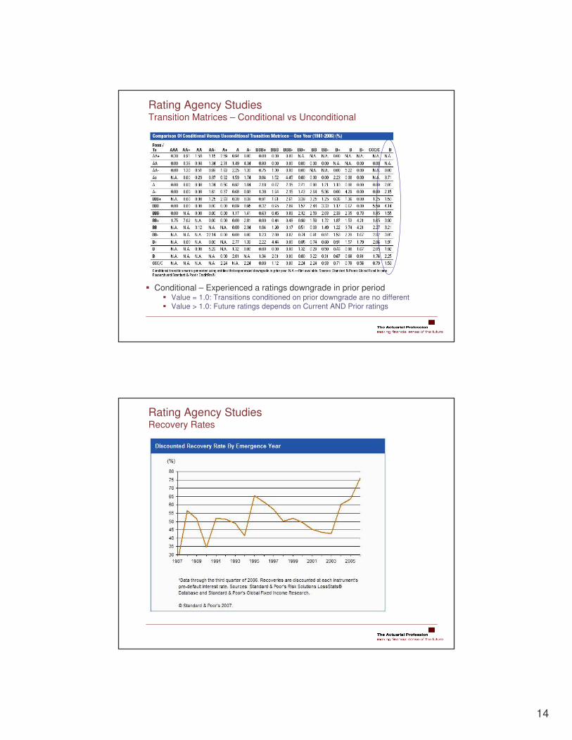
Rating Agency Studies Transition Matrices – Conditional vs Unconditional

� Conditional – Experienced a ratings downgrade in prior period � Value = 1.0: Transitions conditioned on prior downgrade are no different � Value > 1.0: Future ratings depends on Current AND Prior ratings

Rating Agency Studies Recovery Rates

15


Speculative Grade (BB+ & lower)

Investment Grade (BBB- & higher)


Ultimate Recovery Rates

Original Rating RecoveryStandard Deviation Observations

Bank Debt 77.5 30.9 1,204 Senior Secured Bonds 62.0 33.3 301 Senior Unsecured Bonds 42.6 34.8 769 Senior Subordinated Bonds 30.3 33.3 469 Subordinated Bonds 29.2 34.2 394 Junior Subordinated Bonds 19.1 30.6 49 Standard & Poor's Global Fixed Income Research & Standard & Poor's CreditPro

� Recovery rates are conditional on the level of debt seniority� Higher security � greater expected recovery� Standard deviation High

� Measurement does not ‘neutralise’ impact of economic cycle

16

Rating Agency Studies Default Rate vs Recovery Rate

Inverse relationship between Probability of Default and Recovery Rate

Rating Agency Studies Impairment Rates – A.M. Best Studies

� A.M. Best rated U.S. domiciled insurance companies � General Corporate Bond Default Rates are inappropriate for insurance:

� Unique regulatory and accounting environments� Relatively few insurers issue public debt

� Impairment is a wider category of financial duress than default� Impairment often occurs when insurer able to meet policyholder obligations

� Regulators sufficiently concerned about future solvency to intervene

� � Impairment rates > Default rates for a given rating

� Definition of Impairment� Financially Impaired Company (“FIC”) - First official regulatory action taken

� Ability to conduct normal insurance operations is adversely affected� Capital and Surplus inadequate to meet legal requirements� General financial condition has triggered regulatory concern

� State Actions include: � Regulatory Supervision, Rehabilitation, Liquidation, Receivership etc. � and any other action that restricts a company’s freedom to conduct its insurance

business as normal

17

Topics








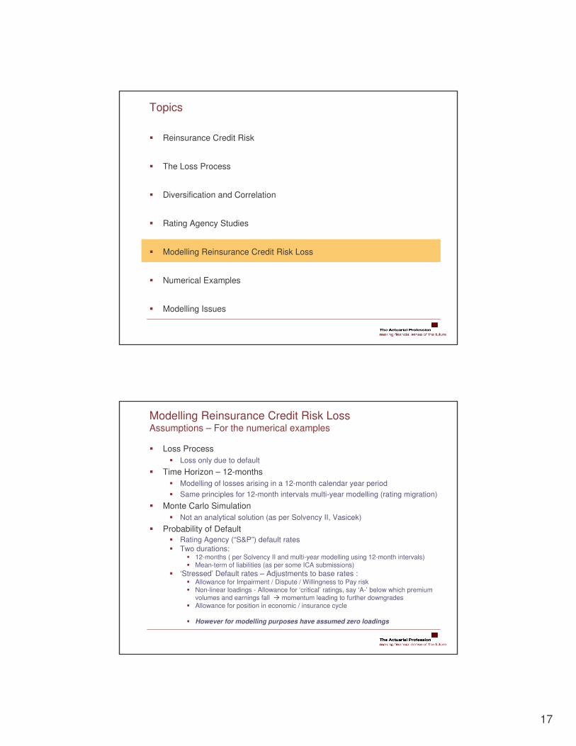
Modelling Reinsurance Credit Risk Loss Assumptions – For the numerical examples

� Loss Process� Loss only due to default

� Time Horizon – 12-months� Modelling of losses arising in a 12-month calendar year period� Same principles for 12-month intervals multi-year modelling (rating migration)

� Monte Carlo Simulation� Not an analytical solution (as per Solvency II, Vasicek)

� Probability of Default� Rating Agency (“S&P”) default rates� Two durations:

� 12-months ( per Solvency II and multi-year modelling using 12-month intervals)� Mean-term of liabilities (as per some ICA submissions)

� ‘Stressed’ Default rates – Adjustments to base rates :� Allowance for Impairment / Dispute / Willingness to Pay risk� Non-linear loadings - Allowance for ‘critical’ ratings, say ‘A-’ below which premium

volumes and earnings fall � momentum leading to further downgrades� Allowance for position in economic / insurance cycle

� However for modelling purposes have assumed zero loadings

18

Modelling Reinsurance Credit Risk Loss Assumptions – For the numerical examples

� Loss Given Default� Not easy to determine – see sample from Final Dividend % (London Market)� Use of E(LGD) values (by Rating) in “GDV Solvency II paper (Dec 05)”� Assumed to be variable with a Beta Distribution ( Standard Deviation 15%)

� Probability of Default and Loss Given Default – Independent� Reinsurer Asset Returns are Multi-variate Normal

Examples of Paid Recoveries - Finalised Settlements

Name Final DividendAndrew Weir 49.7%Anglo American 100% +BNIB 100.0%Fremont (UK) 38.3%Hawk 23.0%ICS Re 88.8%Pine Top 24.9%RMCA Re 93.0%Scan Re 80.5%Stockholm Re 36.4%NEMGIA 37.6%

Source: Bulmer R. et al; Reinsurance Bad Debt Provisions for GI companiesParty - Supplementary Advisory Note of Oct 2005 (Appendix 3); GIRO WP, (Jan 2000)

Modelling Reinsurance Credit Risk Loss Data Inputs – Information at individual Reinsurer level

� Exposure (assumed to be Constant) – Separate for Prior and Current Year� Credit Rating

� Probability of Default (duration)� Loss Given Default

� Variable (No) – LGD Fixed %� Variable (Yes) – LGD Beta Distribution( α,β)

No. of Reinsurers 16 Recoveries 10,000,000 Expected Loss 158,027

INPUT DATA Years Prior Severity Variable Yes

Reinsurer Recoveries Rating PD E(Loss) SD(Loss) Alpha (αααα) Beta (ββββ)Reinsurer A 100,000 A- 0.530% 55.0% 15.0% 5.50 4.50 Reinsurer B 200,000 BBB 1.520% 58.0% 15.0% 5.70 4.13 Reinsurer C 300,000 BB 6.990% 60.0% 15.0% 5.80 3.87 Reinsurer D 400,000 A- 0.530% 55.0% 15.0% 5.50 4.50 Reinsurer E 200,000 A- 0.530% 55.0% 15.0% 5.50 4.50 Reinsurer F 400,000 BBB 1.520% 58.0% 15.0% 5.70 4.13 Reinsurer G 600,000 BB 6.990% 60.0% 15.0% 5.80 3.87 Reinsurer H 800,000 A- 0.530% 55.0% 15.0% 5.50 4.50 Reinsurer I 300,000 A- 0.530% 55.0% 15.0% 5.50 4.50 Reinsurer J 600,000 BBB 1.520% 58.0% 15.0% 5.70 4.13 Reinsurer K 900,000 BB 6.990% 60.0% 15.0% 5.80 3.87 Reinsurer L 1,200,000 A- 0.530% 55.0% 15.0% 5.50 4.50 Reinsurer M 400,000 A- 0.530% 55.0% 15.0% 5.50 4.50 Reinsurer N 800,000 BBB 1.520% 58.0% 15.0% 5.70 4.13 Reinsurer O 1,200,000 BB 6.990% 60.0% 15.0% 5.80 3.87 Reinsurer P 1,600,000 A- 0.530% 55.0% 15.0% 5.50 4.50

19

Modelling Reinsurance Credit Risk Loss Data Inputs – Default Probabilities (after Smoothing)

PD vs Rating

-

500.0

1,000.0

1,500.0

2,000.0

2,500.0

3,000.0

3,500.0

4,000.0

4,500.0

AAA AA+ AA

AA- A+ A A-

BBB+ BBB

BBB- BB+ BB

BB- B+ B

B-

CCC/C

Actual

Fitted

Term 3 Curve y = exp(a+b.RC)

Rating RC Actual Fitted Log-Actual Log-Fitted WeightsAAA 1 9.0 4.1 2.1972 1.4186 0AA+ 2 7.0 6.4 1.9459 1.8489 0AA 3 0.1 9.8 -2.3026 2.2791 0AA- 4 21.0 15.0 3.0445 2.7094 1A+ 5 26.0 23.1 3.2581 3.1397 1A 6 32.0 35.5 3.4657 3.5700 1A- 7 35.0 54.6 3.5553 4.0002 1BBB+ 8 100.0 84.0 4.6052 4.4305 1BBB 9 93.0 129.1 4.5326 4.8608 1BBB- 10 194.0 198.6 5.2679 5.2911 1BB+ 11 312.0 305.3 5.7430 5.7213 1BB 12 492.0 469.5 6.1985 6.1516 1BB- 13 762.0 721.9 6.6359 6.5819 1B+ 14 1,204.0 1,110.1 7.0934 7.0122 1B 15 1,947.0 1,706.9 7.5740 7.4424 1B- 16 2,489.0 2,624.7 7.8196 7.8727 1CCC/C 17 3,996.0 4,036.0 8.2930 8.3030 1Units 10,000

SUMMARY OUTPUT

Regression StatisticsR Square 98.812%Adjusted R Square 98.713%SE 20.540%Observations 14

ANOVAdf SS MS F Significance F

Regression 1 42.1188 42.1188 998.3019 6.36671E-13Residual 12 0.5063 0.0422Total 13 42.6251

Coefficients SE t Stat P-value 2.5% 97.5%Intercept 0.9883 15.317% 6.4525 3.14858E-05 0.6546 1.3220X Variable 1 0.4303 1.362% 31.5959 6.36671E-13 0.4006 0.4599

� Curve y = exp (a + b.RC) – Rating given values from 1 to 17. (Similar to Solvency II calibration)

� Curve Fitting only for shorter durations. Often omitting highest ratings � use implied ‘smoothed’ values.

� Adjusted R ~ 98%. t-distribution statistics OK. Standardised Residuals ?

Modelling Reinsurance Credit Risk Loss Correlation – Cholesky Matrix decompositionCORRELATION MATRIX

No. 1 2 3 4 5 6Reinsurer A 1 1.00 0.50 0.50 0.25 0.25 0.25Reinsurer B 2 1.00 0.50 0.25 0.25 0.25Reinsurer C 3 1.00 0.25 0.25 0.25Reinsurer D 4 1.00 0.25 0.25Reinsurer E 5 1.00 0.25Reinsurer F 6 1.00CHOLESKY MATRIX

No. 1 2 3 4 5 61 1.00 0.00 0.00 0.00 0.00 0.002 0.50 0.87 0.00 0.00 0.00 0.003 0.50 0.29 0.82 0.00 0.00 0.004 0.25 0.14 0.10 0.95 0.00 0.005 0.25 0.14 0.10 0.16 0.94 0.006 0.25 0.14 0.10 0.16 0.14 0.93

TRANSPOSE CHOLESKY MATRIXNo. 1 2 3 4 5 6

1 1.00 0.50 0.50 0.25 0.25 0.252 0.00 0.87 0.29 0.14 0.14 0.143 0.00 0.00 0.82 0.10 0.10 0.104 0.00 0.00 0.00 0.95 0.16 0.165 0.00 0.00 0.00 0.00 0.94 0.146 0.00 0.00 0.00 0.00 0.00 0.93

ORIGINAL MATRIX - CHECKNo. 1 2 3 4 5 6

1 1.00 0.50 0.50 0.25 0.25 0.252 0.50 1.00 0.50 0.25 0.25 0.253 0.50 0.50 1.00 0.25 0.25 0.254 0.25 0.25 0.25 1.00 0.25 0.255 0.25 0.25 0.25 0.25 1.00 0.256 0.25 0.25 0.25 0.25 0.25 1.00

The pair-wise correlations between 1,2 and 3 are higher (50%) than the others (25%)

� Cholesky Matrix is used to generate ‘correlated’ standard normals from ‘independent’ standard normals

� Original Matrix needs to be ‘Positive Definite’ – not all matrices work

� Product of the Cholesky Matrix and its Transpose equals the Original Matrix

20

Modelling Reinsurance Credit Risk Loss Multi-year Modelling considerations

� Default Probabilities vary over time – ‘Probability Drift’� Good credit rating � higher probability of downgrade than upgrade

� Over time higher rated companies have larger probability of transitioning to lower ratings than is the case over 12-months only.

� Mean reversion in credit ratings

Global Average Transition Rates (1981-2006) (%) - 1 YearFrom/To AAA AA A BBB BB B CCC/C D NR AAA 88.34 7.84 0.47 0.09 0.09 - - - 3.17 AA 0.59 87.31 7.54 0.57 0.06 0.10 0.02 0.01 3.79 A 0.05 2.00 87.39 5.47 0.40 0.15 0.02 0.06 4.46 BBB 0.01 0.15 3.98 84.17 4.14 0.73 0.16 0.24 6.42 BB 0.03 0.06 0.22 5.18 75.71 7.20 0.84 1.07 9.69 B - 0.05 0.18 0.30 5.78 72.77 4.10 4.99 11.83 CCC/C - - 0.26 0.39 1.10 11.15 47.49 26.29 13.34

Global Average Transition Rates (1981-2006) (%) - 3 YearsFrom/To AAA AA A BBB BB B CCC/C D NR AAA 68.39 18.98 2.55 0.40 0.12 0.03 0.03 0.09 9.41 AA 1.41 66.46 18.06 2.38 0.41 0.25 0.02 0.10 10.92 A 0.10 4.57 67.34 12.21 1.52 0.62 0.11 0.32 13.21 BBB 0.04 0.47 9.09 60.55 8.06 2.33 0.43 1.32 17.72 BB 0.05 0.10 0.81 11.33 43.82 11.87 1.54 5.92 24.57 B 0.01 0.07 0.45 1.30 11.01 37.08 4.34 17.04 28.71 CCC/C - - 0.30 1.06 2.43 14.25 13.57 42.61 25.78


� Stochastic exposures becomes more important� Variance of the underlying variables increase over time

� Ratings Momentum exist� Markov Process for transition rates – a convenient modelling approach

� i.e. conditional probability distribution of future states depends only on the current state and not prior states.

� Often used for multi-year modelling of future states - MT = (M1)T

� Where MT = T-year transition matrix

� Empirical evidence suggests otherwise

� Correlated Credit migration � Can use Asset Return correlation framework to determine future ratings of a

company� i.e. the rating changes of any two reinsurers are more likely to move together either

upwards or downwards - rather than being independent processes

� A convenient mathematical representation of economic or insurance cycle impacts on reinsurers

� Consistent with the loss default process (assuming asset correlation)

21


� Correlated Credit migration

Adjusted Transition Matrix (re-spreading of NR)1 Year

From/To AAA AA A BBB BB B CCC/C D AAA 88.34% 7.84% 2.76% 0.53% 0.53% 0.00% 0.00% 0.00%AA 0.59% 87.31% 11.00% 0.83% 0.09% 0.15% 0.03% 0.01%A 0.05% 2.00% 87.39% 9.51% 0.70% 0.26% 0.03% 0.06%BBB 0.01% 0.15% 3.98% 84.17% 9.42% 1.66% 0.36% 0.24%BB 0.03% 0.06% 0.22% 5.18% 75.71% 15.88% 1.85% 1.07%B 0.00% 0.05% 0.18% 0.30% 5.78% 72.77% 15.93% 4.99%CCC/C 0.00% 0.00% 0.26% 0.39% 1.10% 13.68% 58.28% 26.29%

Credit Migration Thresholds

Current BBB t=1 D CCC B BB BBB A AA AAAZ -2.82 -2.51 -2.00 -1.19 1.73 2.95 3.72 + InfinityΦΦΦΦ(.) 0.24% 0.60% 2.27% 11.69% 95.86% 99.84% 99.99% 100.00%

-4.0

-3.7

-3.4

-3.1

-2.8

-2.5

-2.2

-1.9

-1.6

-1.3

-1.0

-0.7

-0.4

-0.1 0.2

0.5

0.8

1.1

1.4

1.7

2.0

2.3

2.6

2.9

3.2

3.5

3.8

Z

Pro

babi

lity

BBBBBB AAAD CCC AAA

Topics








22

Numerical Examples Some Results – 16 Reinsurers as previously described OUTPUTS

Exposure 10,000,000 10,000,000 10,000,000 10,000,000 10,000,000 10,000,000No. Reinsurers 16 16 16 16 16 16Average Rating As Given As Given As Given As Given As Given As GivenCorrelation 0% 25% 50% 0% 25% 50%Mean Term 4 4 4 1 1 1No. Simulations 10,000 10,000 10,000 10,000 10,000 10,000Stress Load 0% 0% 0% 0% 0% 0%

CreditLoss CreditLoss CreditLoss CreditLoss CreditLoss CreditLossEC(VaR 99.5%) 1,218,583 1,675,993 2,329,250 742,709 839,581 963,792as % Exposure 12.2% 16.8% 23.3% 7.4% 8.4% 9.6%EC(TVaR 99.5%) 1,395,832 2,045,597 3,130,242 910,275 1,093,465 1,453,602as % Exposure 14.0% 20.5% 31.3% 9.1% 10.9% 14.5%

Minimum 0 0 0 0 0 0Maximum 2,255,585 3,152,566 4,798,956 1,706,195 1,912,611 3,578,554Expected 157,230 156,978 156,381 21,107 22,135 23,110Std Dev 287,674 340,268 422,968 107,820 119,783 143,783

10.0 %ile 0 0 0 0 0 020.0 %ile 0 0 0 0 0 030.0 %ile 0 0 0 0 0 040.0 %ile 0 0 0 0 0 050.0 %ile 0 0 0 0 0 060.0 %ile 0 0 0 0 0 070.0 %ile 134,494 0 0 0 0 080.0 %ile 338,950 252,720 124,527 0 0 090.0 %ile 604,829 640,051 608,555 0 0 095.0 %ile 786,723 886,391 990,414 51,578 0 099.0 %ile 1,192,029 1,530,445 2,036,799 637,558 676,659 728,21999.5 %ile 1,375,812 1,832,972 2,485,631 763,816 861,717 986,90299.9 %ile 1,644,649 2,494,736 3,968,448 994,438 1,281,578 1,737,091100.0 %ile 2,255,585 3,152,566 4,798,956 1,706,195 1,912,611 3,578,554

Numerical Examples Some Results – 16 Reinsurers ‘A’ rated – 1 year and 4 years OUTPUTS

Exposure 10,000,000 10,000,000 10,000,000 10,000,000 10,000,000 10,000,000No. Reinsurers 16 16 16 16 16 16Average Rating A A A A A ACorrelation 0% 25% 50% 0% 25% 50%Mean Term 4 4 4 1 1 1No. Simulations 10,000 10,000 10,000 10,000 10,000 10,000Stress Load 0% 0% 0% 0% 0% 0%

CreditLoss CreditLoss CreditLoss CreditLoss CreditLoss CreditLossEC(VaR 99.5%) 766,342 858,361 1,091,418 189,134 191,624 122,406as % Exposure 7.7% 8.6% 10.9% 1.9% 1.9% 1.2%EC(TVaR 99.5%) 955,221 1,143,465 1,596,704 442,287 478,171 435,931as % Exposure 9.6% 11.4% 16.0% 4.4% 4.8% 4.4%

Minimum 0 0 0 0 0 0Maximum 1,338,558 1,976,112 3,021,969 1,180,514 1,016,423 1,281,835Expected 22,977 24,764 24,881 2,490 2,617 2,273Std Dev 109,581 125,224 153,297 35,241 38,463 36,404

10.0 %ile 0 0 0 0 0 020.0 %ile 0 0 0 0 0 030.0 %ile 0 0 0 0 0 040.0 %ile 0 0 0 0 0 050.0 %ile 0 0 0 0 0 060.0 %ile 0 0 0 0 0 070.0 %ile 0 0 0 0 0 080.0 %ile 0 0 0 0 0 090.0 %ile 0 0 0 0 0 095.0 %ile 142,524 128,863 0 0 0 099.0 %ile 627,190 700,237 799,973 0 0 099.5 %ile 789,319 883,125 1,116,299 191,624 194,242 124,67999.9 %ile 1,113,006 1,340,567 2,002,843 560,834 663,513 637,175100.0 %ile 1,338,558 1,976,112 3,021,969 1,180,514 1,016,423 1,281,835

23

Topics








Modelling Issues Issues (and Solutions)

� Assumptions for:� Probability of Default (setting “Stressed levels”) � Loss Given Default � Asset (or Default Correlation)� Dependencies

� Amongst the above e.g. PD and LGD; or Value of Asset Return and LGD � Other variables – insurance loss and default rate

� Monte Carlo Sampling error:� Problem for highly rated portfolios and for high loss percentiles (~Capital)

� e.g. probability of default = 0.05% � average one default per 2,000 simulations

� Especially for very lumpy exposures� Error term decreases as N-0.5 (N – No. of simulations) � Need to either:

� Run a very large number of simulations� Use Monte Carlo acceleration methods (i.e. ‘variance reduction techniques’)

� Methods:� Stratified Sampling, Low-Discrepancy sequences, Control Variates etc.

24

Modelling Issues Issues (and Solutions)

� Multi-variate Normal distribution:� May be reasonable for non-financial corporate sector� Could be issue for the insurance sector:

� Correlation between lines of business� Interdependence within the industry - reinsurance � Shared exposures to aggregate industry losses (Large Cats, Systemic issues)

� Multi-variate t-distribution � ‘Fatter’ Tails (perhaps more realistic)

� VaR as a Risk Measure� An issue – linked to the Monte-Carlo sampling error� Especially lumpy exposures� TVaR a better risk measure

the modelling of reinsurance credit risk (2) 031007 · the modelling of reinsurance credit risk 2-5...

Documents