The Microstructure of Currency Markets: an Empirical Model of Intra-day Return and Bid-Ask Spread Behavior

Paolo PasquarielloΘ

Stern School of Business New York University

Revision July 9th 2001

Abstract

This paper analyzes the intra-day relationship between bid-ask spreads and “market” return volatility for quotes posted in a truly global “around-the-clock” market setting, the one for the U.S. Dollar/Deutschemark exchange rate. We are able to identify a statistically and economically significant “Reverse U-shaped” pattern in the bid-offer spread in 1996. Tests of the stability and ordering of “market” volatility, performed across several different fractions of the day, reveal that variances of intra-day returns are heterogeneous and ordered, declining around the Asian lunch break, increasing steadily during the London morning trading hours, peaking at the opening of New York to subsequently fall with the closing of the European markets. Results also indicate that “market” volatility is significantly higher during intra-day versus overnight periods. Then, we introduce a structural model that attempts to explain those empirical regularities by capturing some currency-specific features of the data: possibly asymmetric and stochastic trading cost structure, discrete directional updates and parameters’ temporal heterogeneity, and by relating the bid-ask spread to two different sources of variation: trading costs and market risk. We evaluate these components via GMM using a set of convenient unconditional intra-day moments implied by the basic configuration of the model. Analysis of the resulting estimated patterns reveals that trading costs play a significant role in explaining the intra-day variability of bid and offer currency returns. Inventory considerations appear to be more relevant in the trading morning and by London’s closing, while the perceived risk of arrival of informed trades seems more likely to affect the dealers’ cost structure during the late morning/early afternoon in London, when the bid-ask spread is highest. The contribution of the “true” currency risk to the total variability of the posted bid and ask quotes’ returns is not surprisingly highest at the opening of the European markets. Jumps are more likely to occur during the London morning hours and less likely by the end of the day. Additionally, the estimated upward jump size is higher than the estimated discrete downward adjustment. This evidence suggests that during 1996 central banks unsuccessfully attempted to resist the devaluation trend of the Deutschemark versus the dollar.

JEL Classification: C51, F31 Keywords: Market Microstructure; Exchange Rate; Bid-Ask Spread; GMM ΘPh.D. candidate at the Stern School of Business. Please address comments to the author at the Leonard N. Stern School of Business, New York University, Kaufman Management Education Center, Suite 9-180, 44 West 4th Street, New York, NY 10012-1126, or through email: ppasquar@stern.nyu.edu. This paper has benefited from the comments of Viral Acharya, Stephen Figlewski, Richard Lyons, Arun Muralidhar, Latha Ramchand, Alex Shapiro, Amit Sinha, Marti Subrahmanyam, and the seminar participants at the 2001 MFA Annual Conference, and at the 2001 EFMA Annual Conference. I am especially grateful to Angelo Ranaldo for many insightful discussions on the topic and to Joel Hasbrouck for introducing me to the discipline of Market Microstructure and making available the data on which this research is based. The usual disclaimer applies.

2

1. Introduction Microstructure theory often views the evolution of asset prices over short intervals of time as

affected by systematic or unsystematic long-run updates and transient cost components related to the

particular market in which trading occurs. These costs are alternatively interpreted as arising from

inventory control considerations, asymmetric information and order processing.1 Schwartz (1988)

identifies four classes of variables the literature focuses on as determinants of bid-ask spreads in

financial markets: activity, risk, information and competition. Ho and Stoll (1980, 1981, 1983) show

that uncertainty in the order flow limits dealers’ ability to maintain their optimal inventory position.

Consequently, as in Amihud and Mendelson (1980), increasing order arrival variability would increase

the bid-ask spread. Tinic (1972), Stoll (1979) and Hamilton (1978) hypothesize instead a direct

relationship between the bid-ask spread and the intrinsic risk of holding a security. Several more

recent studies relate information asymmetries between “informed” and “liquidity” traders to trading

costs in securities’ markets. Glosten and Milgrom (1985) and Hasbrouck (1988) reveal that if dealers’

perceived exposure to private information rises, the bid-ask spread would then widen. Few

researchers (e.g. Hamilton (1978)) have also focused on the intensity of competition among traders

as a source of downward pressure on bid and offer quotes’ spreads. Data access constraints limited

the empirical studies on assessing the statistical significance of these issues predominantly to equity

markets. However, recent availability of high-frequency observations has made it possible to apply

tests of microstructure trading theories to the vast foreign exchange market (as in Lyons 1995, 1996).

This study looks at the U.S. Dollar/Deutschemark (DEM/$) as a currency traded in a truly global

“around-the-clock” market setting, and identifies a statistically and economically significant “Reverse

U-shaped” pattern in the intra-day bid-offer spread from quotes there posted in 1996. Tests of the

stability and ordering of “market” volatility, performed across several different fractions of the day,

reveal that intra-day returns variances are heterogeneous and ordered, rising from after the lunch

break in Asian markets until the early afternoon, in correspondence with the simultaneous opening

of New York and the post-meridian phase of trading in London, and subsequently declining. Results

also indicate that “market” volatility is significantly higher during intra-day versus overnight periods.

To address the issue of whether the behavior of the bid-ask spread is related to the temporal profile

of return volatility, we model bid and ask quote-return dynamics. The chosen structure, similar in

principle to Hasbrouck (1999), incorporates not only some of the key microstructure effects that are

prominent in the literature (stochastic, temporally heterogeneous and possibly asymmetric costs of

market-making that include clearing, information and inventory factors) but also several specific

1 For a comprehensive guide to the most influential theoretical work in Market Microstructure, we direct the

reader to Maureen O’Hara’s (1995) popular compendium.

3

features of currency markets, in particular the existence of discrete directional jumps affecting the

“true” expected price process. GMM estimates of intra-day parameters’ evolution and size show that,

consistently with Lyons’ (1995) findings, both trading costs and “intrinsic” shocks are important in

explaining the time-varying variability of bid and offer currency returns.2 Nonetheless, their relative

significance appears to fluctuate during the day, with inventory considerations being more relevant in

the Asian morning and London’s closing trading hours, and the “true” currency return volatility

affecting the dealers’ cost structure in the early afternoon. Jumps appear to be more likely to occur

during the London morning and less likely by the end of the day, while the estimated upward jump

size is higher than the estimated discrete downward adjustment, suggesting that during 1996 central

banks unsuccessfully attempted to resist the devaluation trend of the DEM versus the dollar.

The paper is organized as follows. The next section characterizes statistically a sample of half-hourly

DEM/$ exchange rate quotes and presents relevant empirical evidence on bid-ask spreads and noon

mid-quote return variance that motivates the modeling effort of this study. A parsimonious

theoretical structure is then presented in Section 3, and estimated in Section 4. A discussion of the

results ensues. A brief summary concludes in Section 5.

2. A Statistical Analysis of the Bid-Ask Spread in the DEM/$ Market 2-1 The Foreign Exchange Markets The foreign exchange market is probably the most active financial market in the world. Amounts

traded are huge, with over one trillion dollars in transactions executed each day, so is the frequency

and intensity of trading.3 This paper examines bid and ask quotes for the DEM/$ in 1996. The

DEM/$ exchange rate is a truly global 24-hours-a-day market setting, where quotes posted by

London-based traders compete with prices in New York or Frankfurt, and so we treat it in this

paper, rather than as a sequence of regional markets, as suggested instead by Hsieh and Kleidon

(1996). Nonetheless, regional patterns are still going to emerge and matter in our analysis, as we will

show in greater detail in the next sections. The structure of the DEM/$ (now Euro/$) market, as of

any other actively traded currency, strongly differs from the ones of most equity and futures markets.

Following Bessembinder (1994), we briefly focus on its three main aspects: organization, the specific

2 Lyons’ analysis, although including quantities and transaction prices, is nevertheless limited to quotes

observed on just five trading days, on the week of August 3-7 1992, from 8:30 a.m. to 1:30 p.m. Eastern

Standard Time, too short a period to generalize his results. Moreover, by introducing artificial “opening” and

“closing” trading hours, Lyons’ study does not address the trading continuity issues we deal with in this paper. 3 The web site of Olsen and Associates, http://www.olsen.ch, reports this and other interesting facts about

currency markets that we use in this paper.

4

characteristics of the traded asset, and the nature of the relevant information flows. As compared

with the centralized, order-driven specialist system used on the New York Stock Exchange (NYSE),

for example, the wholesale currency markets are typically decentralized, quote-driven continuous

dealer markets. This decentralized structure implies the absence of a centralized transaction reporting

system for executed trades and of a centralized Clearing-House. Although many currency trades

occur directly between dealers, still a portion of them is executed through brokers that effectively

serve as de facto information clearing houses. Although most equity issues and futures contracts are

traded on markets with routinely daily openings and closings, foreign exchange markets remain

practically always active, except for weekends and few bank holidays, when a smaller amount of

quotes is usually posted by dealers. While NYSE specialists engage in market-making activities as an

institutional feature of their role, currency dealers are generally large or medium commercial and

investment banks whose other business activities might also require extensive currency transactions.

The most prominent currency market makers are located in primary financial centers, like London,

Zurich, New York, Tokyo and Hong Kong. They operate as dealers, trading with each other as well

as with non-bank customers, including institutional investors, hedge funds, big and small

corporations and multinational firms. Dealers indicate their willingness to trade by posting quotes on

electronic systems provided by outside vendors, as Reuters or Telerate. However, those quotes are

just indicative, i.e. do not commit the dealer to execution. Actual transactions are completed privately

or through electronic communication, as in the Reuters 2000 Dealing System. Whereas equity

valuations depend on a wide range of both macro-economic and firm (or industry)-specific

information, currency valuation arises mainly from macro-economic considerations. The resulting

nature and frequency of the information flow in the currency markets might reduce market-makers’

likelihood of suffering a loss to better-informed traders. Nonetheless, foreign exchange markets are

characterized by the activity of additional players, i.e. central banks and governments. The monetary

authorities of a country periodically intervene in domestic and foreign currencies with the clear intent

of directing the current and future transaction prices, in order to serve several political or economic

agendas. Inflation pressures, competitiveness of local industries, flows of trade and international

currency commitments are among the most likely motivations for routine interventions by central

bankers. Although central banks do not have a hedge in the size of the transactions for some of the

most actively traded currencies as in the past, their power of “moral suasion” still appears to

condition the activity and expectations of traders in the global currency arena. In any case, the

presence of these players adds a layer of strategic interaction, not usually faced by equity market

makers, to the opportunity set of currency dealers. While stock specialists treat their net equity

position as inventory, with the domestic currency as the numeraire, forex dealers have an alternative

in choosing which currency (if either) should represent the numeraire and which should instead

5

measure the inventory. Moreover, equity prices and futures are always quoted in specific units of

currency per equity share or tick respectively. On the contrary, terms of quotation in exchange rate

markets are a matter of convention, which varies across currencies, and which, as suggested by

Bessembinder (1994), may even affect the distributional properties of the resulting bid-ask spreads.

In particular, although most major currencies are quoted against the U.S. dollar, i.e. prices are the

quantity of the foreign currency per dollar, few exceptions are the Euro and some British

Commonwealth currencies that are typically quoted in quantity of U.S. dollars per unit of the foreign

currency. Finally, currency markets do not impose a pre-specified minimum tick to the quoted prices,

as in equity and futures markets. Market makers can choose the desired fineness of the posted

quotes, depending on the thinness of the order flow and the cost structure they face. This makes the

implying transaction costs fully endogenous. Detailed data on intra-day transactions in this market

were not easily available in the past, as banks and other dealers have no obligation to report their

private transactions. However, the development of computer and communications technology over

the past few years has made available live data at shorter and longer time intervals during the trading

hours. This availability is particularly interesting in the 24-hour-a-day currency markets. It begins

every business morning (Greenwich Mean Time, GMT) in the Asian markets, and increases rapidly,

as Singapore and Hong Kong join Tokyo and Sidney. There is then an abrupt decline of activity at

4:00 a.m. as these markets break for lunch. Trading picks up again at 5:00 a.m. and remains strong

throughout the morning, as London and the rest of Europe replace the Asian centers. The overlap of

the New York and European markets in the afternoon produces the peak of daily volume activity. A

steady decline then follows as the U.S. markets close during the evening.

2-2 Data Characteristics and Bid-Ask Spread Analysis This section performs a statistical analysis of the intra-day dynamics of the bid-ask spread in the

DEM/$ exchange rate market that motivates the development of the model we present and estimate

in the remainder of the paper. The sample we use in this study consists of bid and ask quotes

prevailing on the DEM/$ exchange rate on 262 regular U.K. business days in 1996, reported in

Deutschemark (DM) per U.S. dollar. The data are collected from Reuters on a half-hour frequency

by Olsen & Associates in the HFDF II data set. Olsen & Associates utilizes a filtering process to

remove false prices, or “noise”, due to mis-typing errors by traders. Although those quotes are not

necessarily posted by the same dealer, competition among market makers, investors’ desire to trade at

the displayed rates, and knowledge of transaction prices allow us to interpret the available bids and

asks as being formulated by a single dealer. Figure 1 shows the behavior of the DEM/$ extracted

daily series computed as noon GMT mid-quote, that corresponds roughly to the middle of the

London trading day.

6

Fig. 1. Daily DEM/$ Exchange Rate Mid-quote as of noon, GMT, 1996.

The Deutschemark experienced a devaluating pressure against the dollar during the year, although

through some wide fluctuations around the depreciation trend. Prices are quoted here to four

decimal places, i.e. with a tick size of 0.0001, e.g. 1.4325 DEM per one dollar. Incidentally we

observe that the tick size reported here is practically imposed by the particular information system

collecting the data. This observation is important, insofar as it implies that the clustering

phenomenon in spreads and quotes reported by the literature might be instead less intense.4 In fact

for actively traded currencies, as in the case of DEM/$ in 1996, traders increase the finesse of the

quotes on their screens to the fifth or sixth decimal figure.5 As already emphasized in the previous

sub-section, the bid and ask quotes registered from the Reuters terminals are just indicative, i.e. do

not necessarily represent prices at which transactions really occurred at or around the time the quotes

were recorded. Moreover, these quotes are not necessarily the “best” bid and ask on the market at

that particular time.6 Nonetheless, Goodhart, Ito, and Payne (1996) and Evans (1998, 1999) compare

4 See for example Bessembinder (1994) and, more recently, Hasbrouck (1999). From an economic perspective,

clustering arises when market participants agree (explicitly or implicitly) to a price increment that is coarser than

any technically mandated minimum. It has also been suggested (Christie and Schultz, 1994) that quote

clustering might reflect a collusive behavior among dealers. 5 For example, in the case of DEM/$ exchange rate, dealers’ screens would report, for levels around 1.55, bid-

ask quotes like “6075-6092”, meaning “1.556075-1.556092”, thus attenuating the supposed clustering around 5

and 10 ticks of the bid-ask spread. 6 Hasbrouck (1999) adds that these quotes are usually dominated by bids and asks appearing on the screens of

the inter-dealer market and on electronic trading systems such as the Reuters D2000-2 platform.

DEM/$ Exchange Rate Mid-Quote at 12:00 Noon GMT - 1996

1.4200

1.4400

1.4600

1.4800

1.5000

1.5200

1.5400

1.5600

1.5800

1/1/96 2/1/96 3/1/96 4/1/96 5/1/96 6/1/96 7/1/96 8/1/96 9/1/96 10/1/96 11/1/96 12/1/96

DEM

/$

7

indicative quotes collected by Olsen & Associates with short samples of spot transaction prices, and

find that the resulting indicative spread overestimates the magnitude of the transaction bid-ask

spread and the relevance of clustering, but, and most importantly for our study, appears to be a good

proxy for the intraday dynamics of transaction prices and spreads. Additionally, Bollerslev and

Melvin (1994) observe that reputation effects prevent the posting of quotes at which a bank would

not subsequently be willing to trade.

In order to analyze the intra-day behavior for the bid-ask spread of DEM/$, we partition each day

into 24 consecutive 60-minutes intervals and then calculate mean bid-ask spreads. Following Chan,

Chung and Johnson (1995), we at first define the DEM/$ volatility as the absolute logarithmic return

resulting from the bid-ask midpoint series. Finally, all variables are transformed into standardized

deviates, by subtracting from each the observed mean for the day and dividing by the standard

deviation for the day for the spread and the return, respectively. Table 1 reports the mean values for

the standardized spread (SSPREAD) and volatility (SVOL) for each 60-minutes interval of the day.

Table 1 Mean Values of the Standardized Volatility and Bid-Ask Spread for DEM/$

Exchange Rate from January 1 1996 to December 31 1996 – GMT° Time of the Day SVOL^ SSPREAD^

0:00 – 1:00 0.0230 -0.2328 1:00 – 2:00 -0.2967 -0.3867 2:00 – 3:00 -0.3535 -0.3439 3:00 – 4:00 -0.4890 -0.1636 4:00 – 5:00 -0.2968 0.0369 5:00 – 6:00 -0.1467 -0.1612 6:00 – 7:00 0.0091 0.1194 7:00 – 8:00 0.0063 0.1085 8:00 – 9:00 -0.0333 0.1006 9:00 – 10:00 -0.1243 0.1455 10:00 – 11:00 -0.0613 0.0774 11:00 – 12:00 0.0672 0.1213 12:00 – 13:00 0.2231 0.0930 13:00 – 14:00 0.4339 0.1272 14:00 – 15:00 0.4463 0.1102 15:00 – 16:00 0.4214 0.2183 16:00 – 17:00 0.4459 0.1677 17:00 – 18:00 0.2710 0.0496 18:00 – 19:00 0.1499 0.0609 19:00 – 20:00 -0.0333 0.1103 20:00 – 21:00 -0.2081 -0.0634 21:00 – 22:00 -0.2708 -0.0242 22:00 – 23:00 -0.2363 -0.1401 23:00 – 0:00 0.0533 -0.1312

°The sample consists of 6288 observations on DEM/$ exchange rate on one-hour frequency for regular U.K. business days in 1996. ^The Standardized variable is defined as (Xit - µi)/Si , where Xit is the raw variable, µi is the mean for the day, and Si is the standard deviation for the day.

The bid-ask spread reveals a statistically significant intra-day pattern. It is lowest at the beginning of

the day, gradually increasing after the Asian lunch break until London’s early afternoon before finally

8

declining during the New York evening. As evident from Figure 2, this pattern contradicts the U-

shape in spreads typically documented for stocks, for example in Brock and Kleidon (1992) and

Chang, Chung and Johnson (1995) among others, in organized exchanges, like the NYSE, that are

characterized by formal opening and closing hours.

Fig. 2. Intra-day DEM/$ SSPREAD and SVOL, 1996, one-hour partition. The lines are smoothed interpolations of the variables’ estimates.

Interestingly enough, the intra-day pattern of volatility seems to mimic that of the standardized

spread. This evidence does not prima facie support most of the existing information models (Glosten

and Milgrom (1985), Kyle (1985), Admati and Pfeiderer (1992), just to quote a few) in which market-

makers, facing informed and liquidity agents, increase spreads with lower volume and return volatility

so that the gains from trading with the uninformed compensates for the losses to the informed.7 The

results of Table 1 and Figure 2 suggest instead that the bid-ask spread increases when there is more

uncertainty surrounding the proxy for “true” currency values, as measured by SVOL for mid-quotes.8

As long as higher volatility induces increasing order imbalance in the dealers’ inventory, the bid-ask

spread might widen, thus confirming early observations by Madhavan and Smith (1993) and

Hasbrouck and Sofianos (1993) for NYSE stocks. The evidence on mimicking behavior of

standardized volatility and bid-ask spread is insensitive to the particular time partition (60 minutes)

we originally chose. We repeat the same analysis on an interval that roughly corresponds to the

London trading day (5:00 a.m. to 19:00 p.m., GMT), and report the results in Table 2 and Figure 3.

7 In addition, if liquidity traders are allowed to choose when to enter the market, the resulting order clustering

induces more market depth, lower transaction costs and increasing competition among informed traders. For

more on this topic, see O’Hara (1995). 8 The patterns observed at the beginning of the day appear nonetheless to be consistent with models of

asymmetric information, see for example Foster and Viswanathan (1994), which predict that trading costs,

hence the bid-ask spread, are high when volatility is high at the start of the trading session, i.e. when informed

traders are asymmetrically informed.

Standardized DEM/$ Volatility - January 1 1996 - December 31 1996

-0.6

-0.4

-0.2

0

0.2

0.4

0.6

0:00 2:24 4:48 7:12 9:36 12:00 14:24 16:48 19:12 21:36 0:00

Time of the Day

SVol

Standardized Bid-Ask Spread DEM/$ - January 1 1996 - December 31 1996

-0.5

-0.4

-0.3

-0.2

-0.1

0

0.1

0.2

0.3

0:00 2:24 4:48 7:12 9:36 12:00 14:24 16:48 19:12 21:36 0:00

Time of the Day

SSpr

ead

9

Table 2 Mean Values of the Standardized Volatility and Bid-Ask Spread for

DEM/$ Exchange Rate from January 1 1996 to December 31 1996 - GMT Time of the Day SVOL^ SSPREAD^

5:00 -0.1702 -0.3411 5:30 -0.1372 0.0190 6:00 -0.1366 0.2235 6:30 0.0255 0.0150 7:00 -0.0029 0.1522 7:30 0.0340 0.0651 8:00 -0.0157 0.0301 8:30 0.0669 0.1753 9:00 -0.1413 0.1801 9:30 -0.1541 0.1118 10:00 -0.0944 0.0435 10:30 -0.0844 0.1120 11:00 -0.0392 0.1108 11:30 0.0782 0.1353 12:00 0.0686 0.0908 12:30 0.1144 0.0964 13:00 0.3287 0.0470 13:30 0.3168 0.2064 14:00 0.5393 0.0381 14:30 0.3522 0.1826 15:00 0.5424 0.2154 15:30 0.4072 0.2207 16:00 0.4474 0.3325 16:30 0.5686 0.0051 17:00 0.3219 0.0922 17:30 0.3304 0.0089 18:00 0.2130 0.0518 18:30 0.1577 0.0683 19:00 0.1441 0.1189

^The sample consists of 12576 observations on DEM/$ exchange rate on half-hour frequency for regular U.K. business days in 1996. The Standardized variable is defined as (Xit - µi)/Si , where Xit is the raw variable, µi is the mean for the day, and Si is the standard deviation for the day.

Again, the standardized spread picks up simultaneously with an increase of SVOL from 5:00 a.m. to

8:00 a.m., is stable for most of the morning, rises in the afternoon at the opening of New York and

reaches the highest level at around 3:00 p.m. GMT before declining with the close of the American

trading floors.

Fig. 3. Intra-day DEM/$ SSPREAD and SVOL, 1996, 30-minutes partition. The lines are smoothed interpolations of the variables’ estimates.

Standardized DEM/$ Spread & Volatility - 1996 - London Trading Day

-0.4

-0.3

-0.2

-0.1

0

0.1

0.2

0.3

0.4

0.5

0.6

4:55 6:07 7:19 8:31 9:43 10:55 12:07 13:19 14:31 15:43 16:55 18:07Time of the Day

SVOLSSPREAD

10

2-3 Statistical Analysis of Intra-day Volatility The analysis of the last section suggests that the behavior of intra-day volatility of the underlying

currency process, as measured by absolute returns, might play a relevant role in explaining the

“Reverse U-shaped” profile for the bid-ask spread in DEM/$ quotes. This section examines more

accurately a different measure of volatility, the sample standard deviation of hourly mid-quote returns

for the DEM/$ exchange rate in 1996, and formally tests the null hypothesis of stable variation

within the day. Figure 4 presents the sample volatility for intra-day hourly mid-quote returns

computed as the natural logarithm of the DEM/$ relative value.

Fig. 4. Intra-day DEM/$ sample mid-quote return volatility, 1996, one-hour partition. The line is a smoothed interpolation of the variable’s estimates.

In comparison with the results reported in Figure 2, the increase in return volatility appears more

pronounced during the London trading day, and the evening decline sharper than in the case in

which the return variation is measured by absolute returns. Nonetheless, Figure 4 is generally

consistent with our previous analysis. There is widespread agreement in the empirical literature on

exchange rates that currency markets tend to exhibit daily and weekly “seasonality”. Glassman (1987)

and Bessembinder (1994) report that both bid-ask spreads and absolute returns, as measures of risk,

are usually higher on Fridays than on any other day of the working week. In Table 3 and Figure 5 we

estimate intra-day sample mid-quote return volatility for Mondays to Fridays in 1996. No significant

difference arises from the comparison of the resulting intra-day profiles, all displaying a “Reverse U-

shape”. In particular, the morning patterns are virtually identical across days. Nonetheless, Tuesdays

and Thursdays, not just Fridays, appear to be characterized by higher return volatility at the peak of

daily currency activity, with the overlap of the New York and European markets in the afternoon.9

9 The recurrence of certain economic events (e.g. Fed meetings on Tuesdays) in specific sub-periods of the day

might explain these results.

Sam ple Period-by-Period Return Volatility on the DEM/$ Exchange Rate for 1996

0.04%

0.06%

0.08%

0.10%

0.12%

0.14%

0.16%

0:36 3:00 5:24 7:48 10:12 12:36 15:00 17:24 19:48 22:12Time of the D ay

stde

v

11

Table 3 Sample Return Volatility for DEM/$ Exchange Rate from January 1 1996 to December 31 1996 – GMT^

Measurement Period Total Monday Tuesday Wednesday Thursday Friday 0:00 – 1:00 0.0862% 0.0879% 0.0894% 0.0815% 0.0890% 0.0817% 1:00 – 2:00 0.0673% 0.0573% 0.0606% 0.0845% 0.0578% 0.0735% 2:00 – 3:00 0.0575% 0.0384% 0.0525% 0.0703% 0.0455% 0.0709% 3:00 – 4:00 0.0486% 0.0305% 0.0337% 0.0418% 0.0707% 0.0560% 4:00 – 5:00 0.0665% 0.0520% 0.0574% 0.0746% 0.0463% 0.0914% 5:00 – 6:00 0.0802% 0.0774% 0.1029% 0.0621% 0.0843% 0.0689% 6:00 – 7:00 0.0734% 0.0690% 0.0669% 0.0767% 0.0758% 0.0780% 7:00 – 8:00 0.0875% 0.0718% 0.0950% 0.0936% 0.0758% 0.0996% 8:00 – 9:00 0.0835% 0.0707% 0.1003% 0.0835% 0.0616% 0.0968% 9:00 – 10:00 0.0738% 0.0432% 0.0763% 0.0741% 0.0826% 0.0788% 10:00 – 11:00 0.0803% 0.0712% 0.0892% 0.0836% 0.0917% 0.0626% 11:00 – 12:00 0.1114% 0.0815% 0.0795% 0.1005% 0.1800% 0.0842% 12:00 – 13:00 0.0998% 0.0923% 0.0934% 0.0918% 0.1185% 0.1002% 13:00 – 14:00 0.1214% 0.0954% 0.1027% 0.1046% 0.1194% 0.1707% 14:00 – 15:00 0.1231% 0.1006% 0.1510% 0.0896% 0.1219% 0.1437% 15:00 – 16:00 0.1242% 0.1040% 0.0902% 0.1045% 0.1355% 0.1716% 16:00 – 17:00 0.1443% 0.0898% 0.1779% 0.1175% 0.1732% 0.1468% 17:00 – 18:00 0.1066% 0.0910% 0.1410% 0.1046% 0.0949% 0.0946% 18:00 – 19:00 0.1052% 0.0886% 0.1469% 0.0944% 0.1038% 0.0776% 19:00 – 20:00 0.0841% 0.0881% 0.0734% 0.0723% 0.0962% 0.0864% 20:00 – 21:00 0.0573% 0.0510% 0.0551% 0.0506% 0.0624% 0.0654% 21:00 – 22:00 0.0803% 0.0828% 0.0593% 0.1004% 0.0589% 0.0918% 22:00 – 23:00 0.0770% 0.0876% 0.0558% 0.1066% 0.0423% 0.0783% 23:00 – 0:00 0.1166% 0.0726% 0.1237% 0.0787% 0.0696% 0.1925%

Number of Days 262 53 53 52 52 52 ^The sample consists of 6288 observations on DEM/$ exchange rate on one-hour frequency for regular U.K. business days in 1996.

We next test more formally the equality of variances across J intra-day intervals, i.e. the null

hypothesis H0 : σ21 = σ22 = …. = σ2J , using various non-parametric procedures. The analysis is

initially performed across 4 intra-day periods of 6 hours each. Then, results are reported for each

sub-period in Table 4. The null hypothesis H0 is examined first with the Brown-Forsythe (1974)

modified Levene (1960) test statistic, already utilized in a study by Lockwood and Linn (1990) on

stock market return volatility. The statistic is computed as:

( ) ( ) ( )( )[ ]

= =••

=•

•

= =•

=•••

=

=

−=

−−�

���

�−−=

J

j

n

iij

n

ijijj

jijij

J

j

n

ijij

J

jjj

j

j

j

NDD

nDD

MRD

JJNDDDDnF

1 1

1

1 1

2

1

21

, [ 1 ]

12

where Rij is the return for day i, intra-day period j, M• j is the sample median return for period j

computed over the nj (262) days included in the test, D• j is the mean absolute deviation from the

median for period j and D•• is the grand mean. The statistic in [1] is distributed FJ-1, N-J under the null

hypothesis.

Fig. 5. Intra-day DEM/$ sample mid-quote return volatility, 1996, one-hour partition, Mondays to Fridays. The lines are smoothed interpolations of the variables’ estimates.

In Table 4, the null hypothesis H0 is rejected at any conventional significance level, indicating that

“market” return variance, as measured by the sample mid-quote return proxy, is statistically not

constant across the four intra-day periods and is larger during the London trading day.

In order to identify more precisely the typical intra-day pattern in “market” volatility, the Dij can be

ranked and examined for each day in the sample. Patterns in the Dij ranks allow us to test different

expected orderings among intra-day variances versus a null hypothesis of random ordering, an

analysis typically neglected by traditional statistical approaches.

Table 4 Modified Levene Statistics for Test of the Equality of Variance across Intra-Day Trading Periods

DEM/$ Exchange Rate Mid-Quote – 1996 K Measurement Period Mean Bid-Ask Spread Sample Return Vols # of Days 1 0:00 to 6:00 0.000548 0.167228% 262 2 6:00 to 12:00 0.000614 0.219322% 262 3 12:00 to 18:00 0.000620 0.315387% 262 4 18:00 to 0:00 0.000582 0.193882% 262 F-Test for H0 : σ21=σ22=σ23=σ24 F3,1044(0.01) = 3.80 F^ = 26.231**

** The F-Statistic is significant at the one percent level.

For this purpose, we use a significance test developed by Page (1963). We define ri1 through ri4 as the

ranks from the smallest Dij to the largest Dij in day i. Because we have 4 sub-periods, the number of

possible rankings is 24 (4!). Under the null hypothesis of random ordering of the rij over 262

S am ple S tandard D eviation for the returns on the D E M /$ E xchange R ate - 1996 - D ay-by-D ay D ecom position

0.01%

0.03%

0.05%

0.07%

0.09%

0.11%

0.13%

0.15%

0.17%

0.19%

0.21%

0:36 3:00 5:24 7:48 10:12 12:36 15:00 17:24 19:48 22:12Tim e of th e D ay

stde

v

FridayThursdayW ednesdayTuesdayM onday

13

independent trials, we expect to observe an average frequency for each ordering of 10.91, with a

standard deviation of 3.23.10 If we define hij as the rank under a pre-specified alternative hypothesis,

the Page ordered test statistic L is

= ==

N

i

J

jijij hrL

1 1. [ 2 ]

Thus, the Page test uses the hypothesized ranks (hij ) and the observed ranks (rij,) to produce a

statistic that, for any day i, obtains its maximum value when hij, = rij, (i.e. 30 for J = 4) and its

minimum value when they are instead inversely related (e.g. 20 in our case with J = 4).

Page (1963) provides critical values for the exact distribution of L.11 Here we instead use a modified

version of Page’s test, L*, which is distributed approximately as chi-square with one degree of

freedom,12

)1)(1(])1(312[*

22

2

+−+−=JJNJ

JJNLL . [ 3 ]

We consider four alternative hypotheses, HA1 to HA4, for the observed ordering across intra-day sub-

periods, each of them ex-ante consistent with Figure 4, i.e. implying market volatility rising from the

opening in Asia until the European afternoon, and falling thereafter (1-3-4-2; 1-4-3-2; 2-3-4-1 and 2-

4-3-1 respectively).

10 Assuming, consistently with the null hypothesis, a sequence of 262 independent binomial trials, it then

follows easily that:

[ ] ( ) ( )

[ ] ( )[ ] ( ) ( )=

−

=

−

−⋅−⋅�

���

�=

−⋅⋅���

���

�=

262

1

2622

262

1

262

1#262

#

1262

#

i

ij

ijjj

i

ij

ijj

ppEii

VAR

ppii

E

where #j is the number of cases in which the ordering j is observed, and pj is the ex-ante probability to observe

#j under the null of random ordering (1/4!). 11 Lockwood and Linn (1990) report that the Page test appears to be extremely powerful, especially if an a

priori ordering is believed to exist. 12 In this case, the ordinary use of χ2 tables is equivalent to a two-sided test of the null hypothesis. To

implement instead a one-sided test, as in our case, the probability implying from the chi-square tables needs to

be halved. See Page (1963), pp. 220-224, for more details.

14

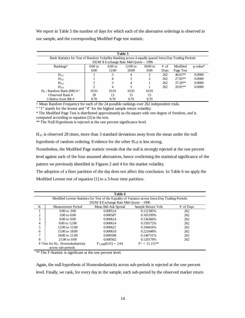
We report in Table 5 the number of days for which each of the alternative orderings is observed in

our sample, and the corresponding Modified Page test statistic.

Table 5 Rank Statistics for Test of Random Volatility Ranking across 4 equally spaced Intra-Day Trading Periods

DEM/$ Exchange Rate Mid-Quote – 1996 Rankings° 0:00 to

6:00 6:00 to 12:00

12:00 to 18:00

18:00 to 0:00

# of Days

Modified Page Test

p-value*

HA1 1 3 4 2 262 46.61** 0.0000 HA2 1 4 3 2 262 27.05** 0.0000 HA3 2 3 4 1 262 37.20** 0.0000 HA4 2 4 3 1 262 20.01** 0.0000

H0 : Random Rank (RR) #^ 10.91 10.91 10.91 10.91 Observed Rank # 28 13 15 15

3 Stdevs from RR # 9.70 9.70 9.70 9.70 ^ Mean Random Frequency for each of the 24 possible rankings over 262 independent trials. ° “1” stands for the lowest and “4” for the highest sample return volatility. * The Modified Page Test is distributed approximately as chi-square with one degree of freedom, and is computed according to equation [3] in the text. ** The Null Hypothesis is rejected at the one percent significance level.

HA1 is observed 28 times, more than 3 standard deviations away from the mean under the null

hypothesis of random ordering. Evidence for the other HAs is less strong.

Nonetheless, the Modified Page statistic reveals that the null is strongly rejected at the one percent

level against each of the four assumed alternatives, hence confirming the statistical significance of the

pattern we previously identified in Figures 2 and 4 for the market volatility.

The adoption of a finer partition of the day does not affect this conclusion. In Table 6 we apply the

Modified Levene test of equation [1] to a 3-hour time partition.

Table 6 Modified Levene Statistics for Test of the Equality of Variance across Intra-Day Trading Periods

DEM/$ Exchange Rate Mid-Quote – 1996 K Measurement Period Mean Bid-Ask Spread Sample Return Vols # of Days 1 0:00 to 3:00 0.000514 0.121385% 262 2 3:00 to 6:00 0.000587 0.105199% 262 3 6:00 to 9:00 0.000614 0.136366% 262 4 9:00 to 12:00 0.000614 0.159172% 262 5 12:00 to 15:00 0.000621 0.194416% 262 6 15:00 to 18:00 0.000619 0.221648% 262 7 18:00 to 21:00 0.000598 0.146751% 262 8 21:00 to 0:00 0.000562 0.120179% 262 F-Test for H0 : Homoskedasticity

across sub-periods F7,2088(0.01) = 2.64 F^ = 21.151**

** The F-Statistic is significant at the one percent level.

Again, the null hypothesis of Homoskedasticity across sub-periods is rejected at the one percent

level. Finally, we rank, for every day in the sample, each sub-period by the observed market return

15

volatility and report, in Table 7, the number of times for which each of the 8 possible ranks has been

observed.

Table 7 Intra-Day Trading Periods classified by Mid-Quote return volatility rankings over successive days

DEM/$ Exchange Rate Mid-Quote – 1996 Rankings 0:00 to

3:00 3:00 to

6:00 6:00 to

9:00 9:00 to 12:00

12:00 to 15:00

15:00 to 18:00

18:00 to 21:00

21:00 to 0:00

# of Days

Low Vol 32 64 31 27 20 18 31 39 262 2 41 36 36 28 27 22 28 44 262 3 31 37 26 30 22 32 45 39 262 4 49 35 31 32 18 25 31 41 262 5 35 36 39 43 26 25 33 25 262 6 28 25 29 32 36 39 45 28 262 7 26 14 37 40 49 37 32 27 262

High Vol 20 15 33 30 64 64 17 19 262 χ2 Independence Test : T^ = 218.32* p-value = 0.0000

* The χ2-Statistic is significant at the one percent level (with 49 degrees of freedom), and is computed according to footnote 16 in the text.

The resulting matrix reveals a higher concentration of high volatility observations during the London

trading day, and a higher concentration of low volatility rankings in the Asian markets’ afternoons. A

chi-square Independence test rejects at the one percent level the null hypothesis of random ordering

for the 64 combinations of volatility rankings and 3-hour sub-periods.13

To summarize, the results of this section indicate that:

a) the Bid-Ask spread for DEM/$ quotes is characterized by a statistically significant “Reverse U-

shaped” intra-day pattern;

b) the observed intra-day spread variation is economically significant as well: for a single “round-

trip” $ 100 Mil. transaction at a level of DEM/$ 1.5000, the average difference in the dealer’s fee

between the 12-to-15 pm interval and the Asian morning hours, 0.000107, is translated into

approximately $ 7300, or about 18% of the noon GMT mean bid-offer spread;

c) the “market” return volatility, as a proxy for market risk measured over mid-quote intra-day

returns, reveals a statistically significant “seasonal” daily pattern that is not explained by random

chance. Variation in DEM/$ returns declines around the Asian lunch break, then increases

13 The test compares the actual number of observations (Aij) for each cell with the expected range (Eij) under

the selected null hypothesis, in this case of random ordering. Hence, the null implies an average of 32.75

(8*262/64) observations per combination. A test statistic is then computed as:

( )= =

−=

8

1

8

1

2

i j ij

ijij

EEA

T .

Under the null, T is distributed as chi-square with (J-1)(I-1) degrees of freedom.

16

steadily during the London morning trading hours, peaks at the opening of New York to then

fall with the closing of the European markets.

Although poignant, the statistical analysis we just performed does not substitute for an economic

interpretation of our findings and eventually does not offer a satisfying explanation of Figure 6

below. It remains in fact to clarify

a) what, if any, is the relationship between the fluctuations of the bid-ask spread and the intra-day

behavior of the “market” volatility;

b) how much of the “market” volatility dynamics is explained by the variation of the underlying

“true” currency process and how much is instead resulting from fluctuations in trading costs;

c) whether the variability of the “true” underlying currency process and/or trading cost

considerations, both probably embedded in our estimates of “market” variation, help explaining

the puzzling “Reverse U-shaped” spread we clearly see in Figure 6.

Fig. 6. Intra-day DEM/$ sample mid-quote return volatility and bid-ask spread, 1996, three-hour partition.

These unanswered questions are investigated in the remainder of this study.

3. The Model 3-1 Motivation The purpose of this section is to construct, and eventually estimate, a model for the bid and ask

intra-day return, return volatility, and the bid-ask spread for exchange rates that captures the main

characteristics of the data we presented in the last section, while incorporating at the same time some

of the features of past and current theoretical contributions to market microstructure literature.

Schwartz (1988) identifies four classes of variables that appear to determine bid-ask spreads in

financial markets: activity, risk, information and competition. As suggested by Stoll (1989), those

S a m p le R e tu r n V o la t il i t y a n d M e a n B id -A s k S p r e a d o n th e D E M /$ E x c h a n g e R a t e f o r 1 9 9 6 - 8 In tr a -D a y P e r io d s

0 .0 0 0 5 0 0

0 .0 0 0 5 2 0

0 .0 0 0 5 4 0

0 .0 0 0 5 6 0

0 .0 0 0 5 8 0

0 .0 0 0 6 0 0

0 .0 0 0 6 2 0

0 .0 0 0 6 4 0

1 :3 0 4 :3 0 7 :3 0 1 0 :3 0 1 3 :3 0 1 6 :3 0 1 9 :3 0 2 2 :3 0T im e o f t h e D a y

0 .0 0 6 %

0 .0 5 6 %

0 .1 0 6 %

0 .1 5 6 %

0 .2 0 6 %

0 .2 5 6 %

R e tu rn V o la t i l i ty

B id - A s k S p re a d

S p r e a d V o la t i l i t y

17

variables induce three types of costs eventually faced by a dealer: order processing costs, inventory-

holding costs, and adverse information costs.

More intense trading activity may lead to lower spreads because of economies of scale in trading

costs. Researchers have shown that volume, number of shares traded and number of transactions are

significant determinants of the bid-ask spread in stock markets.14 Inventory control models, like in

Ho and Stoll (1980, 1981, 1983), show that uncertainty in the arrival of buy and sell orders drives

dealers away from their optimal inventory position. As in Amihud and Mendelson (1980), when the

trader approaches his desired inventory book, the bid-ask spread would be reduced. In short, if

economies of scale predominate, then we should observe an inverse relationship between spreads

and trading activity. If we rely on the “market” volatility we estimated using mid-quotes as a proxy

for intensity of trading, then the evidence reported in the last section, especially in Figures 2 and 6,

appears to refute this hypothesis. However, sample return volatility depends on the degree of

variation of both the underlying “true” currency process and the related trading costs. Hence, Figures

2 and 6 alone do not help us disentangle the two effects on the observed bid-ask spread “Reverse U-

shaped” intra-day behavior. Other researchers, like Tinic (1972), Stoll (1978), and Hamilton (1978),

describe a direct relationship between the bid-ask spread and the risk of holding a security, whether

systematic or unsystematic. Although this hypothesis appears more consistent with our empirical

findings, the issue of distinguishing properly the risk component related to the “true” asset price

process and the risk component implied by the trading activity itself however remains. Glosten and

Milgrom (1985) and Hasbrouck (1988) show that the spread might be positively related to the

amount of information coming to the market. The trader’s perceived exposure to private information

determines how he will respond to large versus small orders, and to arrivals of market-generated and

other publicly available information. As the dealer attributes a positive probability to the order being

generated from informed traders, the spread widens at times of the day during which substantial

informational changes are more likely, hence when the “true” asset volatility is higher. In the context

of the global currency markets, these intra-day sub-periods correspond to the Asian morning, the

opening of the trading day in London, and the subsequent activity following from the U.S. markets.

From a different perspective, Saar (2000) investigates the role of demand uncertainty, i.e. uncertainty

about preferences and endowments of the investors’ population, in introducing information content

to the order flow. He shows that demand uncertainty increases both the bid-ask spread and price

volatility, consistently with our findings in Tables 4 and 6 and Figures 2 and 3.

14 For an exhaustive review of empirical and theoretical literature on the components of the bid-ask spread, see

Stoll (1989), McInish and Wood (1992) and O’Hara (1995).

18

Finally, few researchers15 have reported an inverse relationship between the level of competition and

the observed bid-ask spreads. This explanation does not appear to be satisfactorily for the case of

foreign exchange intra-day patterns, given the evidence presented here. In fact, it is exactly at the

peak of the daily activity in the London afternoon, when both European and American dealers are in

the market, that the widest spread is recorded, as clear from Figure 3.

From this discussion, it clearly emerges the need to identify sources of variation in the bid and ask

intra-day returns, accounting for the inventory costs and information components, and to relate them

to the period-by-period behavior of the recorded bid-ask spread. This is the task we reserve to the

next section.

3-2 The Basic Structure We construct a dynamic model for bid and ask intra-day returns that incorporates a stochastic

process for the underlying “true” exchange rate, a random market-making cost and a specific feature

of foreign exchange markets, discrete jumps. This model will allow us to identify two different

possible sources of variation in bid and ask intra-day returns, trading costs (due to inventory and/or

competition) and market volatility (as a proxy for intrinsic risk and/or information asymmetry).

The model is very similar in nature to the one of Hasbrouck (1999), but distinguishes itself from it in

three main aspects. First, we focus our attention on logarithmic returns, instead of levels, in order to

pursue a different estimation strategy, GMM instead of Gibbs Sampling. Second, we ignore

discreteness and clustering of quotes. Discreteness of quotes arises as a restriction of bid and ask

prices to a fixed grid. Clustering is the tendency of quotes and spreads to lie on certain multiples of a

basic tick size. Bessembinder (1994) and Hasbrouck (1999) exhaustively describe both phenomena

and document their empirical relevance in currency markets. We observed in the past section that

discreteness and clustering of quotes and spreads might arise from a tick size being imposed to the

DEM/$ figures by the particular information system that collects the data.

Although we do not make any specific claim on the significance of this limitation on the empirical

evidence available in the literature on clustering, we choose to focus this paper on an analysis of the

relationship between the bid-ask spread and the volatility of bid and ask intra-day returns, with the

intent to maintain the parsimony of the selected specification.

Third, as already mentioned, we introduce the possibility for the “true” underlying currency process

to be affected by a discrete upward or downward jump. Discrete movements in currency quotes may

be induced by the release (or the revision) of fundamental macro-economic information or the

occurrence of major political events, but also by the purposeful intervention of domestic and foreign

15 See Hamilton (1976, 1978) and Branch and Freed (1977), for example.

19

central banks. In any case, the introduction of systematic jump risk appears to be one of the most

popular and successful tools used by the literature16 to capture the conditional and unconditional

leptokurtosis and skewness typically observed in log-differenced exchange rates.

We define the latent variable St as the efficient (or “true”) currency price (e.g. DEM per dollar)

arising at the end of the trading day conditional on all public information available at that time. In

what follows, we indicate any raw variable in upper cases, and the corresponding natural logarithm in

lower cases. We assume that st = Ln(St) changes over time according to the following process:

)()()()()( 1 tgtytutsts kj

kj

kju

kj

kj +++= − µ , [ 4a ]

( ))(,0~)( 2 kNtu uiid

kj σ [ 4b ]

( ))(~)( ktyiid

kj λ Poisson [ 4c ]

��

−≤≥

=)(10

)(0)(

2

1

kpgkpg

tg kj prob with

prob with [ 4d ]

where t = 1,2,…..,262 stands for a specific day in the sample, j = 1/24,2/24,…..,1 is a specific

fraction of the day and k = 1,2,…..,8 is one of the eight three-hour sub-periods we divide a trading

day in,17 as in Table 6 and Figure 6; µu is a time-homogeneous drift in the exchange rate, while ukj(t)

reflects updates to the “true” value of DEM/$ resulting from the release of publicly available

information; ykj(t) is the number of discrete random jump updates, distributed as a Poisson variate.

λ(k) controls the frequency of arrival of events, its mean number and its variance. The binomial

variable gkj(t) determines the direction of the jump, with period-varying probability p(k) of being

positive. For the purposes of this paper, we consider the probability of a discrete jump to occur and

of a jump to be upward as independent from each other and from the public information update

ukj(t).

16 See Bates (1996) for a review of some of the main modeling solutions adopted in the financial literature to

represent the behavior of exchange rates, and for evidence on DEM/$ exchange rate over the period 1984 to

1991. 17 Hence, t + j = t +1/24 corresponds to 0:00 a.m. of day t (and sub-period 1), t + 5/24 corresponds to 4:00

a.m. of day t (and sub-period 2), and so on.

20

Dealers are assumed to face a non-negative stochastic cost of market-making, C. As mentioned in

section 3-1, C incorporates any fixed or marginal (i.e. per trade) cost incurred by the currency dealer

in posting (non-binding) quotes.

The randomness in the determinants of these costs, whether arising from inventory considerations or

asymmetric information, represents an additional source of variation for bid and ask intra-day

returns. The cost C is not necessarily symmetric,18 thus reflecting the fact that in specific market

circumstances or moments of the day quoting a bid price may be “more (or less) expensive” than

being on the ask side.

We assume that a randomly extracted forex dealer (from a population of market-makers) posts the

following raw bid and ask quotes at the j-th fraction of the t-th day, in the k-th sub-period:

)()()( tCbtStBid kj

kj

kj ⋅= [ 5a ]

)()()( tCatStAsk kj

kj

kj ⋅= . [ 5b ]

Cb (< 1) and Ca (> 1) represent the “mark-up” practiced by the market-maker on the “true”

currency price as a compensation for inventory carrying costs, information asymmetry risk, and

market risk. As mentioned earlier on, no tick and rounding restrictions to the posted quotes are

considered here.

We model the stochastic nature of these costs by assuming that:19

( ) ( ) )()()()()()( 11 tktcatcatCaLntCaLn kjcaca

kj

kj

kj

kj ηµ +=−≡− −− [ 6a ]

( ) ( ) )()()()()()( 11 tktcbtcbtCbLntCbLn kjcbcb

kj

kj

kj

kj ηµ +=−≡− −− , [ 6b ]

18 Evidence on asymmetric bid-ask spread, based on analysis of daily observations, is reported by Bossaerts and

Hillion (1991), among others. 19 This choice is consistent with the dynamic implications of assuming lognormal trading costs, as in Blume and

Stambaugh (1983), Smith (1994) and, more recently, Hasbrouck (1999). In fact, for example in the case of bid

costs Cb, if we instead assume that Ln[Cbkj(t)] ~ iid N[mcb(k) , s2cb(k)], it follows that [Ln(Cbkj(t)) – Ln(Cbkj-1(t))]

is distributed as i.i.d. N[Ikj(t)(mcb(k) - mcb(k)), Ikj(t)(s2cb(k) + s2cb(k-1)) + (1 - Ikj(t))(2s2cb(k))], where Ikj(t) = 0 for j

and (j-1) in the same interval k, and 1 otherwise. Equation [6b] would then just impose the additional

restriction that µcb = Ikj(t)(mcb(k) - mcb(k)) and σ2cb = Ikj(t)(s2cb(k) + s2cb(k-1)) + (1 - Ikj(t))(2s2cb(k)).

21

where

( )( )

0)(),(),(

)(,0~)(

)(,0~)(

,,,

2

2

≠kkk

kNt

kNt

cbucaucbca

cbiidk

jcb

caiidk

jca

ρρρ

ση

ση

[ 6c ]

Although some of the determinants of market-making costs are known to be serially correlated, the

random cost innovations are assumed to be i.i.d. Nonetheless, we do not exclude a priori the

possibility that updates to public information have an impact on the cost structure (ρu,ca & ρu,cb ≠ 0),

not that there might exists some interaction between the cost of being on the bid or on the offer side

of the market at any point in time (ρca,cb ≠ 0).

If we define:

�

��

�

�=

− )(

)()(

1 tBid

tBidLntr k

j

kjk

jbid [ 7a ]

�

��

�

�=

− )(

)()(

1 tAsk

tAskLntr k

j

kjk

jask [ 7b ]

as the intra-day bid and ask return respectively, our assumptions imply that

)]()([)]()([)( 11 tcbtcbtststr kj

kj

kj

kj

kjbid −− −−−= [ 8a ]

)]()([)]()([)( 11 tcatcatststr kj

kj

kj

kj

kjask −− −−−= [ 8b ]

It also follows from [4], [5] and [6] that the bid-ask spread representation provided by the model is:

���

� −=+

−+

−++

−)()(

1)()(

1)()()(

1 )()()()( tkkj

tkkj

tgtytukj

kj

kjcbcb

kjcaca

kj

kj

kju etCbetCaetSt ηµηµµSpread . [ 9 ]

22

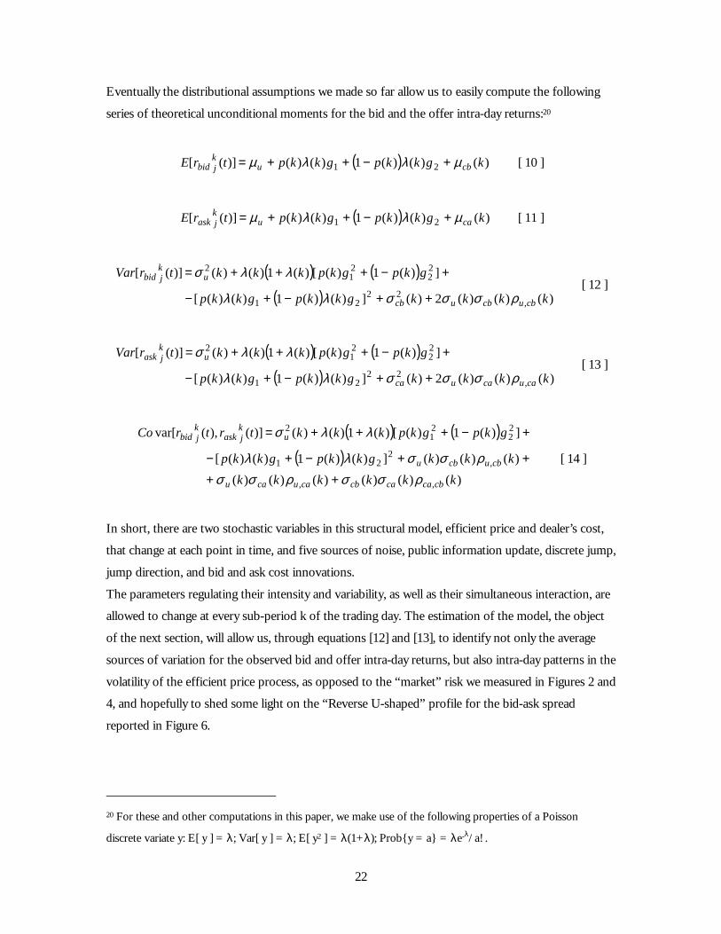
Eventually the distributional assumptions we made so far allow us to easily compute the following

series of theoretical unconditional moments for the bid and the offer intra-day returns:20

( ) )()()(1)()()]([ 21 kgkkpgkkptrE cbukjbid µλλµ +−++= [ 10 ]

( ) )()()(1)()()]([ 21 kgkkpgkkptrE caukjask µλλµ +−++= [ 11 ]

( ) ( )( ) )()()(2)(])()(1)()([

])(1)([)(1)()()]([

,22

21

22

21

2

kkkkgkkpgkkp

gkpgkpkkktrVar

cbucbucb

ukjbid

ρσσσλλ

λλσ

++−+−

+−+++=

[ 12 ]

( ) ( )( ) )()()(2)(])()(1)()([

])(1)([)(1)()()]([

,22

21

22

21

2

kkkkgkkpgkkp

gkpgkpkkktrVar

caucauca

ukjask

ρσσσλλ

λλσ

++−+−

+−+++=

[ 13 ]

( ) ( )( )

)()()()()()()()()(])()(1)()([

])(1)([)(1)()()](),(var[

,,

,2

21

22

21

2

kkkkkkkkkgkkpgkkp

gkpgkpkkktrtrCo

cbcacacbcaucau

cbucbu

ukjask

kjbid

ρσσρσσρσσλλ

λλσ

++

++−+−

+−+++=

[ 14 ]

In short, there are two stochastic variables in this structural model, efficient price and dealer’s cost,

that change at each point in time, and five sources of noise, public information update, discrete jump,

jump direction, and bid and ask cost innovations.

The parameters regulating their intensity and variability, as well as their simultaneous interaction, are

allowed to change at every sub-period k of the trading day. The estimation of the model, the object

of the next section, will allow us, through equations [12] and [13], to identify not only the average

sources of variation for the observed bid and offer intra-day returns, but also intra-day patterns in the

volatility of the efficient price process, as opposed to the “market” risk we measured in Figures 2 and

4, and hopefully to shed some light on the “Reverse U-shaped” profile for the bid-ask spread

reported in Figure 6.

20 For these and other computations in this paper, we make use of the following properties of a Poisson

discrete variate y: E[ y ] = λ; Var[ y ] = λ; E[ y2 ] = λ(1+λ); Prob{y = a} = λe-λ/a! .

23

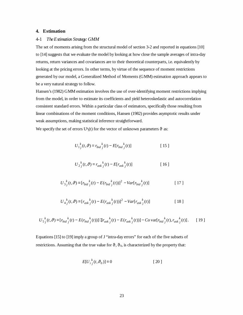
4. Estimation 4-1 The Estimation Strategy: GMM The set of moments arising from the structural model of section 3-2 and reported in equations [10]

to [14] suggests that we evaluate the model by looking at how close the sample averages of intra-day

returns, return variances and covariances are to their theoretical counterparts, i.e. equivalently by

looking at the pricing errors. In other terms, by virtue of the sequence of moment restrictions

generated by our model, a Generalized Method of Moments (GMM) estimation approach appears to

be a very natural strategy to follow.

Hansen’s (1982) GMM estimation involves the use of over-identifying moment restrictions implying

from the model, in order to estimate its coefficients and yield heteroskedastic and autocorrelation

consistent standard errors. Within a particular class of estimators, specifically those resulting from

linear combinations of the moment conditions, Hansen (1982) provides asymptotic results under

weak assumptions, making statistical inference straightforward.

We specify the set of errors Ukj(t) for the vector of unknown parameters ϑ as:

)]([)(),(1 trEtrtU kjbid

kjbid

kj −=ϑ [ 15 ]

)]([)(),(2 trEtrtU kjask

kjask

kj −=ϑ [ 16 ]

)]([))](()([),( 23 trVartrEtrtU k

jbidkjbid

kjbid

kj −−=ϑ [ 17 ]

)]([))](()([),( 24 trVartrEtrtU k

jaskkjask

kjask

kj −−=ϑ [ 18 ]

)](),(var[))](()([))](()([),(5 trtrCotrEtrtrEtrtU kjask

kjbid

kjask

kjask

kjbid

kjbid

kj −−⋅−=ϑ . [ 19 ]

Equations [15] to [19] imply a group of J “intra-day errors” for each of the five subsets of

restrictions. Assuming that the true value for ϑ , ϑ0, is characterized by the property that:

0)],([ 0 =ϑtUE kji [ 20 ]

24

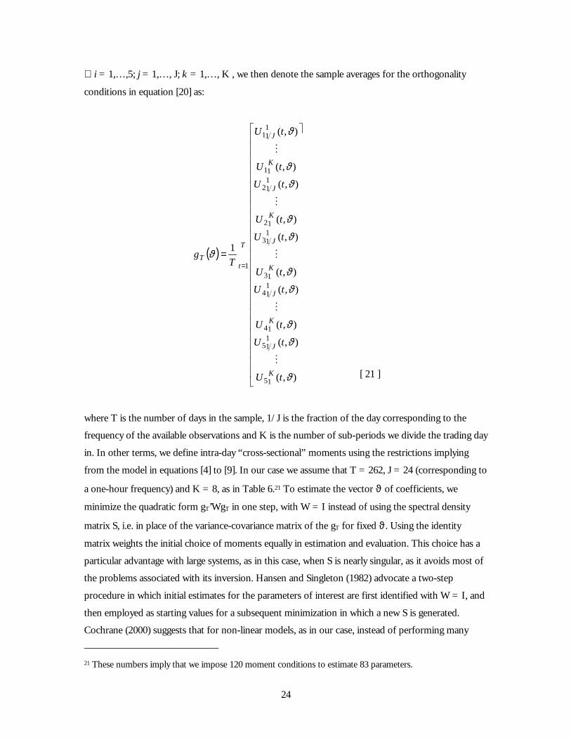
∀ i = 1,…,5; j = 1,…, J; k = 1,…, K , we then denote the sample averages for the orthogonality

conditions in equation [20] as:

( )=

�

�������������������������

�

�

=T

t

K

J

K

J

K

J

K

J

K

J

T

tU

tU

tU

tU

tU

tU

tU

tU

tU

tU

Tg

1

15

115

14

114

13

113

12

112

11

111

),(

),(

),(

),(

),(

),(

),(

),(

),(

),(

1

ϑ

ϑ

ϑ

ϑϑ

ϑ

ϑ

ϑϑ

ϑ

ϑ

�

�

�

�

�

[ 21 ]

where T is the number of days in the sample, 1/J is the fraction of the day corresponding to the

frequency of the available observations and K is the number of sub-periods we divide the trading day

in. In other terms, we define intra-day “cross-sectional” moments using the restrictions implying

from the model in equations [4] to [9]. In our case we assume that T = 262, J = 24 (corresponding to

a one-hour frequency) and K = 8, as in Table 6.21 To estimate the vector ϑ of coefficients, we

minimize the quadratic form gT’WgT in one step, with W = I instead of using the spectral density

matrix S, i.e. in place of the variance-covariance matrix of the gT for fixed ϑ . Using the identity

matrix weights the initial choice of moments equally in estimation and evaluation. This choice has a

particular advantage with large systems, as in this case, when S is nearly singular, as it avoids most of

the problems associated with its inversion. Hansen and Singleton (1982) advocate a two-step

procedure in which initial estimates for the parameters of interest are first identified with W = I, and

then employed as starting values for a subsequent minimization in which a new S is generated.

Cochrane (2000) suggests that for non-linear models, as in our case, instead of performing many

21 These numbers imply that we impose 120 moment conditions to estimate 83 parameters.

25

times a numerical search over gT’(ϑ)WgT(ϑ), minimizing once the original quadratic form with W = I

ensures a quicker convergence and still asymptotically equivalent estimates with better small-sample

properties.22

If we define DT to be a consistent estimator of ∂gT(ϑGMM)/∂ϑGMM, we then have that for our GMM

estimates ϑGMM:

( ) ( )1]'[,0~ˆ −− TTGMM DDNT ϑϑ . [ 22 ]

Finally, the minimized quadratic form q = TgT’(ϑGMM)gT(ϑGMM) allows to test for the overall fit of the

model. When there is the same number of moment equations as there are parameters to estimate, the

model is perfectly identified and testing the validity of the restrictions is clearly redundant. However,

if, as in our case, the parameters are over-identified by the moment equations, those equations imply

substantive restrictions.

As a consequence, if the model that led to the set of moment conditions in the first place is incorrect,

at least some of the sample moment restrictions of equations [15] to [19] will be systematically

different from zero. Hence, T times the minimized value of the one-stage objective function,

distributed χ2 with degrees of freedom equal to d, the number of moments less the number of

estimated parameters23, is a Wald statistic for a test of the d over-identifying restrictions.

4-2 Model Evaluation In this section, we estimate a reduced and the full version of the model of equations [4] to [9] using

the one-stage GMM procedure described in the last sub-section.24

The reduced version assumes that none of the following parameters, σ2u, p, λ, µca, µcb, σ2ca, σ2cb, ρu,ca,

ρu,cb, ρca,cb, changes across four 6-hour sub-periods of the day, with J = 4 and K = 1. Table 8 reports

22 For a more detailed analysis of this and other important issues in GMM estimation, we remand the reader to

the very exhaustive treatment of Cochrane (2000), chapters 11 to 16. 23 In our case, d = 5J – 83 = 37. 24 The quadratic form gT’(ϑ)WgT(ϑ) is minimized using the Generalized Gradient (GRG2) nonlinear

optimization code developed by Leon Lasdon, University of Texas at Austin, and Allan Waren, Cleveland State

University. In order to obtain economically sound parameters’ estimates, some of the variables have been

constrained to assume values in certain ranges. Hence, correlation terms are bounded between -1 and +1,

variances are bounded to be positive, as are the mean model spreads implying from the model.

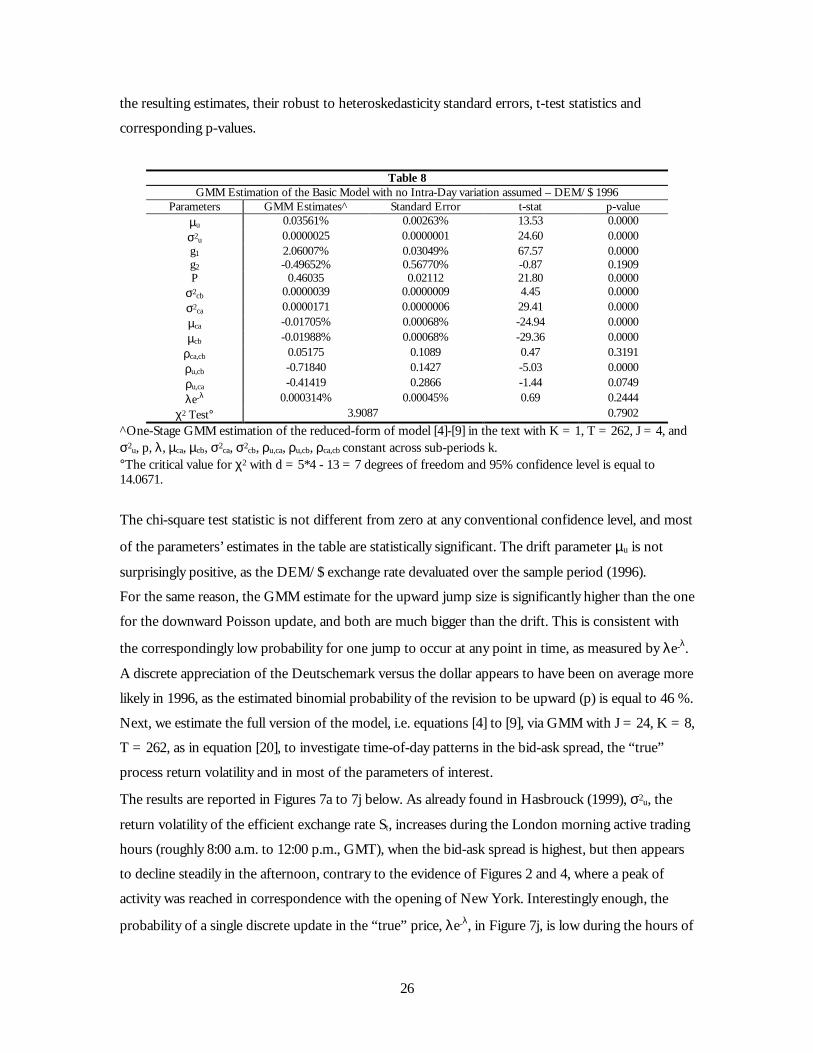
26

the resulting estimates, their robust to heteroskedasticity standard errors, t-test statistics and

corresponding p-values.

Table 8 GMM Estimation of the Basic Model with no Intra-Day variation assumed – DEM/$ 1996

Parameters GMM Estimates^ Standard Error t-stat p-value µu 0.03561% 0.00263% 13.53 0.0000 σ2u 0.0000025 0.0000001 24.60 0.0000 g1 2.06007% 0.03049% 67.57 0.0000 g2 -0.49652% 0.56770% -0.87 0.1909 P 0.46035 0.02112 21.80 0.0000

σ2cb 0.0000039 0.0000009 4.45 0.0000 σ2ca 0.0000171 0.0000006 29.41 0.0000 µca -0.01705% 0.00068% -24.94 0.0000 µcb -0.01988% 0.00068% -29.36 0.0000

ρca,cb 0.05175 0.1089 0.47 0.3191 ρu,cb -0.71840 0.1427 -5.03 0.0000 ρu,ca -0.41419 0.2866 -1.44 0.0749 λe-λ 0.000314% 0.00045% 0.69 0.2444

χ2 Test° 3.9087 0.7902 ^One-Stage GMM estimation of the reduced-form of model [4]-[9] in the text with K = 1, T = 262, J = 4, and σ2u, p, λ, µca, µcb, σ2ca, σ2cb, ρu,ca, ρu,cb, ρca,cb constant across sub-periods k. °The critical value for χ2 with d = 5*4 - 13 = 7 degrees of freedom and 95% confidence level is equal to 14.0671.

The chi-square test statistic is not different from zero at any conventional confidence level, and most

of the parameters’ estimates in the table are statistically significant. The drift parameter µu is not

surprisingly positive, as the DEM/$ exchange rate devaluated over the sample period (1996).

For the same reason, the GMM estimate for the upward jump size is significantly higher than the one

for the downward Poisson update, and both are much bigger than the drift. This is consistent with

the correspondingly low probability for one jump to occur at any point in time, as measured by λe-λ.

A discrete appreciation of the Deutschemark versus the dollar appears to have been on average more

likely in 1996, as the estimated binomial probability of the revision to be upward (p) is equal to 46 %.

Next, we estimate the full version of the model, i.e. equations [4] to [9], via GMM with J = 24, K = 8,

T = 262, as in equation [20], to investigate time-of-day patterns in the bid-ask spread, the “true”

process return volatility and in most of the parameters of interest.

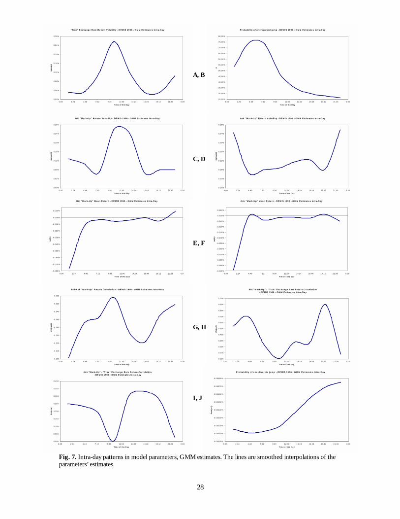
The results are reported in Figures 7a to 7j below. As already found in Hasbrouck (1999), σ2u, the

return volatility of the efficient exchange rate St, increases during the London morning active trading

hours (roughly 8:00 a.m. to 12:00 p.m., GMT), when the bid-ask spread is highest, but then appears

to decline steadily in the afternoon, contrary to the evidence of Figures 2 and 4, where a peak of

activity was reached in correspondence with the opening of New York. Interestingly enough, the

probability of a single discrete update in the “true” price, λe-λ, in Figure 7j, is low during the hours of

27

trading in Asia, but then rises during the day, when both the European central banks and the Fed are

more likely to be active in their “moral suasion” attempts. In the context of the sample period we

examine in this paper, 1996, a downward jump was less likely (1-p) during the early morning hours,

and more likely during the remainder of the day, i.e., exactly when directional updates are more

frequent, according to the estimate for λ in Figure 7j. This fact, together with |g2| being again lower

than |g1|, in turn suggests that in 1996 central banks unsuccessfully attempted to control the

devaluation of the Deutschemark versus the dollar. The trading cost parameters’ estimates also reveal

some noteworthy intra-day patters. Away from the active trading hours, the ask “mark-up” return

volatility is higher. This is however not the case for the bid trading cost volatility σcb, that reaches its

peak between 12:00 p.m. and 3:00 p.m., maybe reflecting the strong selling pressure on the

Deutschemark that characterizes our sample. It is in fact reasonable to suppose that most DEM/$

sales were occurring when London trading activity overlaps with the opening of the currency market

in New York. Consistently with this finding, the mean ask cost return in Figure 7e, µca, shows a more

pronounced increase during the intensely-traded Asian mornings and European afternoons than in

the case of the mean bid trading cost return, µcb. Nonetheless, the intra-day profile of both

parameters, related to the expression for the bid-ask spread of equation [9], suggests that, for fixed

initial Ca and Cb, trading costs increase almost symmetrically with the climbing activity and

competition among dealers that characterizes the Asian mornings and the London afternoons, even

when the spread is rising, and the risk of the underlying “true” currency process is actually declining.

This evidence seems to offer support to the view that, when Asian markets are open or when

London is about to close, inventory considerations play a more significant role in explaining the

intra-day behavior of the bid-ask spread than the systematic and unsystematic risk of the “true”

exchange rate St, a proxy for the dealers’ perceived risk to be exposed to private information.

Correlation between bid and offer cost variables, ρca,cb in Figure 7g, appears to be low, albeit

fluctuating during the day. This result is consistent with Ca and Cb capturing different components of

the trading cost structure of a randomly extracted DEM/$ currency dealer in 1996. ρu,cb and ρu,ca

attempt to capture the interaction between updates to the “true” St resulting from publicly available

news and innovations in the trading cost structure faced by traders. In both cases, the GMM

estimates reveal the existence of a positive relationship between changes in the cost “mark-ups” Ca

and Cb and shocks to the expected currency returns. This interaction is characterized by a very similar

intra-day profile for the bid and the offer side, although by a lower intensity for the buying than for

the selling side of the DEM/$ market in 1996. The correlation increases until the zenith of the Asian

trading day is reached, then falls with the lunch break in Hong Kong, Tokyo and Singapore, rises

again with the opening of London to finally decline with the New York afternoon.

28

A, B

C, D

E, F

G, H

G, H

I, J

Fig. 7. Intra-day patterns in model parameters, GMM estimates. The lines are smoothed interpolations of the parameters’ estimates.

"True" Exchange Rate Return Volatility - DEM/$ 1996 - G MM Estim ates Intra-Day

0.00%

0.04%

0.08%

0.12%

0.16%

0.20%

0.24%

0.28%

0:00 2:24 4:48 7:12 9:36 12:00 14:24 16:48 19:12 21:36 0:00

Tim e of the Day

sigm

a(u)

P robability of one Upw ard jum p - DEM/$ 1996 - GMM Estim ates Intra-Day

25.00%

30.00%

35.00%

40.00%

45.00%

50.00%

55.00%

60.00%

65.00%

70.00%

75.00%

80.00%

0:00 2:24 4:48 7:12 9:36 12:00 14:24 16:48 19:12 21:36 0:00

Time of the Day

p

Bid "Mark-Up" Return Volatility - DEM/$ 1996 - G MM Estim ates Intra-Day

0.00%

0.04%

0.08%

0.12%

0.16%

0.20%

0.24%

0.28%

0:00 2:24 4:48 7:12 9:36 12:00 14:24 16:48 19:12 21:36 0:00

Tim e of the Day

sigm

a(cb

)

B id -Ask "Mark-Up" Return Correlation - DE M/$ 1996 - GMM Estim ates Intra-Day

-0.160

-0.140

-0.120

-0.100

-0.080

-0.060

-0.040

-0.020

0.000

0:00 2:24 4:48 7:12 9:36 12:00 14:24 16:48 19:12 21:36 0:00

Tim e of the Day

rho(

ca,c

b)

Ask "Mark-Up" - "True" Exchange Rate Return Correlation - DEM /$ 1996 - G MM Estim ates Intra-Day

0.000

0.050

0.100

0.150

0.200

0.250

0.300

0.350

0.400

0:00 2:24 4:48 7:12 9:36 12:00 14:24 16:48 19:12 21:36 0:00

T ime of the Day

rho(

u,ca

)

Ask "M ark-Up" Return Vo latility - DEM /$ 1996 - G MM Estim ates In tra-Day

0.00%

0.04%

0.08%

0.12%

0.16%

0.20%

0.24%

0.28%

0:00 2:24 4:48 7:12 9:36 12:00 14:24 16:48 19:12 21:36 0:00

Tim e o f the Day

sigm

a(ca

)

Bid "M ark-Up" - "True" Exchange Rate Return Correlation - DEM /$ 1996 - G MM Estim ates Intra-Day

0.000

0.100

0.200

0.300

0.400

0.500

0.600

0.700

0.800

0.900

1.000

0:00 2:24 4:48 7:12 9:36 12:00 14:24 16:48 19:12 21:36 0:00

Tim e of the Day

rho(

u,cb

)

P robab ility o f one d iscre te jum p - D E M /$ 199 6 - G M M E stim a te s In tra-D ay

0.00000%

0.00010%

0.00020%

0.00030%

0.00040%

0.00050%

0.00060%

0.00070%

0.00080%

0:0 0 2:24 4:48 7:1 2 9:36 12:00 14:24 16:48 19:12 21:36 0:00

T im e o f the D ay

Prob

{x=1

}

B id "Mark-Up" M ean Return - DEM /$ 1996 - G MM E stim ates Intra-Day

-0.080%

-0.070%

-0.060%

-0.050%

-0.040%

-0.030%

-0.020%

-0.010%

0.000%

0.010%

0:00 2:24 4:48 7:12 9:36 12:00 14:24 16:48 19:12 21:36 0:00

Tim e of the Day

m(c

b)

Ask "Mark-Up" M ean Return - DEM /$ 1996 - G M M E stim ates In tra-Day

-0.100%

-0.090%

-0.080%

-0.070%

-0.060%

-0.050%

-0.040%

-0.030%

-0.020%

-0.010%

0.000%

0.010%

0:00 2:24 4:48 7:12 9:36 12:00 14:24 16:48 19:12 21:36 0:00

T im e of th e Day

m(c

b)

29

Using the parameter estimates in equations [12] and [13], we can now measure the contribution of

public-information updates, discrete jumps, trading costs and their interaction to the variance of the

bid and offer intra-day returns, as represented by the model. This is done in Figure 8.25

Fig. 8. Intra-day contribution to bid and offer return variance, GMM estimates. The “true” process variance component for the bid is defined as σ2u, the trading cost component as σ2cb, the jump component as λ(1+λ)[pg21 + (1-p)g22] – [pλg1 + (1-p)λg2]2, and finally the correlation component as 2σuσcbρu,cb. Similar formulas are used for the offer return variance components. Each element is then divided by the estimated totals Var[rbid] and Var[rask], respectively. The lines are smoothed interpolations of the variables’ estimates.

At the beginning of the day, trading costs appear to explain most (around 75%) of the variability of

both bid and ask returns. As long as, at this stage, the contribution of the “true” process return

volatility is low and even slightly declining (as in Figure 7a), and the probability of a discrete jump is

still minimal (see Figure 7j), we are inclined to attribute the cost volatility to the dealer’s inventory

considerations rather than to his perceived risk of being hit by an informed trade.

In light of the behavior of λ and σ2u, the likelihood of this event appears actually to be small. With

the opening of the European markets, the contribution of σ2u to both Var[rbid] and Var[rask] (not

surprisingly) increases. It is in fact during the London morning (8:00 a.m. to 13:00 p.m., GMT) that

most public macro-information information affecting the DEM/$ exchange rate is released, i.e. when

public news updates are most likely to induce variation in the quoted bid and offer prices of the

currency. The importance of the trading cost components again rises with the closing of London,

and the opening of New York. However at this point “true” process volatility is still significant, and

25 In the case of bid returns for example, we define the “true” process variance component as σ2u, the trading

cost component as σ2cb, the jump component as λ(1+λ)[pg21 + (1-p)g22] – [pλg1 + (1-p)λg2]2, and finally the

correlation component as 2σuσcbρu,cb. We then compute, for every sub-period k of the day, the ratio between

each of the components and their total and report their corresponding values in Figure 8. The same is done for

ask returns. The resulting percentage contributions to the total variance display similar, but not identical intra-

day patterns, due to the above-mentioned asymmetry in the estimated bid and ask “mark-up” return volatility.

Decomposition of the Bid return Variance resulting from the Model - DEM/$ 1996 - GMM Estimates Intra-Day

0.00%

10.00%

20.00%

30.00%

40.00%

50.00%

60.00%

70.00%

80.00%

90.00%

100.00%

0:00 2:24 4:48 7:12 9:36 12:00 14:24 16:48 19:12 21:36 0:00

Time of the Day

cont

ribut

ion

(%)

Trading Cost

Correlation

"True" Process

Jump

Decomposition of the Ask return Variance resulting from the Model - DEM/$ 1996 - GMM Estimates Intra-Day

0.00%

10.00%

20.00%

30.00%

40.00%

50.00%

60.00%

70.00%

80.00%

90.00%

100.00%

0:00 2:24 4:48 7:12 9:36 12:00 14:24 16:48 19:12 21:36 0:00

Time of the Day

cont

ribut

ion

(%)

Trading Cost

Correlation

"True" Process

Jump

30

the probability of a discrete event is increasing; hence, it is more likely than before that information

asymmetry considerations are important in explaining the behavior of Cb and Ca. The contribution

of the discrete jump update to return volatility appears minimal, as it never explains more than 0.50%

of Var[rbid] and Var[rask]. In short, the analysis of Figure 8 supports the view that trading costs are

important, although not unique, in explaining the intra-day variability of bid and offer currency

returns. Moreover, the nature of these costs changes during the day, with inventory considerations

more likely to be relevant in the GMT morning and the NY afternoon, and the perceived risk of

arrival of informed trades more significant during the late morning/early afternoon in London.26

In virtue of these results, how well does the model eventually capture the “Reverse U-Shaped” intra-

day pattern for the bid-ask spread in DEM/$ quotes described in Figures 2 and 6? In Figure 9 we

compute, from equation [9], two approximated conditional mean spreads27 for an initial “true” value

26 From a different perspective, the evidence reported here is also consistent with price and quote-formation

dynamics in the foreign exchange markets varying during the day, as the currency is traded more intensely, in

waves, in structurally heterogeneous markets. Moreover, traders may enter the market with dissimilar

motivations (e.g. hedging or speculation) in various sub-periods of the day, thus potentially affecting dealers’

intra-day bid-ask spread profile, as suggested in the pioneering work of Cohen et al. (1978), and later pursued

by Hsieh and Kleidon (1996). Through several simulations of their model, Cohen et al. show that limit orders

with longer horizons (that are more frequently observed in currency markets during the GMT night and the

early morning hours) tend to imply lower spreads and volatility. Hsieh and Kleidon argue that during the early

trading hours of the day, when traders are learning about the structure of the market, in particular about the

identity and behavior of other traders, spreads may be wider to protect them from transacting the currency at

an informational disadvantage. 27 From equation [9], we proxy Ej-1[Spreadkj(t)] by assuming Independence between u, ηca and ηcb with:

][]))(1()([

][][][

)(21)(

1)(

21)(

1)1)(()(

21

1

111

22

21

2 kkkj

kkkj

ggekkkj

kj

kjj

kjj

kjj

cbcbcacauueCbeCaekpekpeS

CbCaESEE

σµσµλσµ +−

+−

−++−

−−−

−⋅−+⋅≈

≈−⋅≈Spread

We also consider the following alternative Taylor approximation, E[g(x,y)] = g(E[x],E[y]), that implies, again

ignoring the assumed co-movements among the stochastic sources of noise in the model:

][][ )(1

)(1

])())(1()()([11

21 kkj

kkj

ekkpekkpkj

kjj

cbcagg

u eCbeCaeSE µµλλµ−−

−++−− −≈Spread .

We finally use as initial value for the spread the mean value from Table 6, Spread(0) = 0.000591 and assume

that Ca(0) = [S0+0.5*Spread(0)]/S0 and Cb(0) = [S0-0.5*Spread(0)]/S0.

31

for S(k), S*(0) = 1.5043, that corresponds to the average sample noon mid-quote for 1996, and then

compare it with the true average spread we calculated in Table 6 of section 2-3.

Fig. 9. Intra-day true and estimated spread. The “true” spread is from Table 6. The model spread is computed from an initial true currency price of 1.5043 using the two approximations derived in footnote 30 of the text. The lines are smoothed interpolations of the variables’ estimates.

The estimated spread size oscillates from a minimum of 0.000346 to a maximum of 0.000698, around

a mean of 0.000554, i.e. slightly lower than the corresponding true values reported in Table 6,

averaging 0.000591. Nonetheless, the model appears to convincingly capture the “Reverse U-shape”

for the bid-ask spread in the DEM/$ quotes in 1996. The difference between the two

approximations used in the estimation is minimal, hence does not affect our conclusions. The

increase in the spread the model allocates in correspondence with the New York opening is smaller

in size than the one resulting from the London morning trading, contrary to the evidence of Tables 4

and 6. Moreover, the estimated spread drops between 9:00 a.m. and 11:00 a.m., another feature

observed in the hour-by-hour analysis of Figure 2 but not in Table 6.

In short, the model performs satisfactorily well in describing the main features of the intra-day cost

of trading in the DEM/$ exchange rate market in the sample period. The bid-ask spread pattern we

identified from the data in section 2 appears to be driven by the dynamics of the cost parameters, µca,

µcb, σ2ca, σ2cb, and their correlations, as well as by the fluctuations of σ2u, measuring the risk of the

expected value of the currency given all available public information.

5. Conclusions The microstructure of foreign exchange markets has been receiving increasing attention from the

financial literature, following the recent availability of “continuous-time” spot data. In this paper

intra-day bid and ask quotes for a truly global “around-the clock” market setting, the U.S.

Dollar/Deutschemark market in 1996, were investigated. We document the statistical and

True versus M ode l B id-Ask spread - D E M /$ 1996 - G M M Estim ates In tra -D ay"True" initial value o f 1 .5043

0 .000300

0 .000340

0 .000380

0 .000420

0 .000460

0 .000500

0 .000540

0 .000580

0 .000620

0 .000660

0 .000700

0 .000740

0:00 2 :24 4 :48 7:12 9:36 12:00 14 :24 16 :48 19:12 21 :36 0 :00T im e o f th e D ay

Spre

ad

T rue S preadTaylor M ode l Spread

Independent M odel Spread

32

economical significance of a “Reverse U-shape” for the bid-offer spread, and test successfully for

existence of heteroskedasticity in the “market” return volatility.

The standardized spread appears to pick up simultaneously with an increase in the noon mid-quote

return volatility from 5:00 a.m. to 8:00 a.m. GMT, is then stable for most of the London trading

morning, rises in the afternoon at the opening of New York and reaches the highest level at around

3:00 p.m. GMT, before declining with the close of the American trading floors.

The behavior of exchange rates and the microstructure of the markets where they are traded differ in

several ways from those of most equity and futures markets. This article introduced a structural

model that attempts to explain those empirical regularities by capturing some currency-specific

features: possibly asymmetric and stochastic trading cost structure, discrete directional updates and

parameters’ temporal heterogeneity, and by relating the bid-ask spread to two different sources of

variation: trading costs and market risk. We evaluate these parameters via GMM using a set of

convenient unconditional intra-day moments implying from the basic configuration of the model.

Analysis of the resulting estimated patterns reveals that trading costs play a significant role in

explaining the intra-day variability of bid and offer currency returns. Inventory considerations appear

to be more relevant in the trading morning and by London’s closing time, while the perceived risk of

arrival of informed trades seems more likely to affect dealers’ cost structure during the late

morning/early afternoon in London, when the bid-ask spread is highest. The contribution of the

“true” currency risk to the total variability of posted bid and ask quotes’ returns is not surprisingly

highest with the opening of the European markets.

Several extensions and refinements of the basic modeling and estimation strategy pursued in this

paper are possible. The distributional assumptions for the sources of systematic and cost updates,

chosen for their wide acceptance in the literature and computational feasibility, are somehow

restrictive, as most studies of security returns suggest that deviations from normality are more

pronounced at higher frequencies.

It is also more likely that the cost and public news shocks would exhibit some form of serial

correlation at those higher frequencies. In our model, we analyzed cross-sectionally fractions of the

trading day and assumed heterogeneity of parameters across sub-periods, ignoring any serial

correlation among the stochastic variables driving the “true” currency process and the dealers’ cost

structure. It would then be a reasonable extension of the model to allow these variables to have

persistent components and auto-regressive dependence.

Broadening the analysis to several different exchange rates would consent to determine whether

some of the results of this paper can be generalized to the currency market in its entirety, or are

instead unique to the specific variable we study, the DEM/$. We reserve these investigations to

future research.

33

References

Admati, A., Pfleiderer, P., A Theory of Intraday Patterns: Volume and Price Variability, 1992, Review

of Financial Studies, 1, pp. 3-40.

Amihud, Y., Mendelson, H., Dealership Market: Market-Making with Inventory, 1980, Journal of

Financial Economics, 8, pp. 31-53.

Amihud, Y., Mendelson, H., Trading Mechanisms and Stock Returns: An Empirical Investigation,

1987, Journal of Finance, 42, pp. 533-553.

Bates, D., Jumps and Stochastic Volatility: Exchange Rate Processes Implicit in Deutsche Mark

Options, 1996, Review of Financial Studies, 9, pp. 69-107.

Bessembinder, H., Bid-Ask Spreads in the Interbank Foreign Exchange Markets, 1994, Journal of

Financial Economics, 35, pp. 317-348.

Blume, M., Stambaugh, R., Bias in Computed Returns: An Application to the Size Effect, 1983,

Journal of Financial Economics, 12, pp. 387-404.

Bollerslev, T., Melvin, M., Bid-ask Spreads and Volatility in the Foreign Exchange Market, 1994,

Journal of International Economics, 36, pp. 355-372.

Bossaerts, P., Hillion, P., Market Microstructure Effects of Government Intervention in the Foreign

Exchange Market, 1991, Review of Financial Studies, 4, pp. 513-541.

Branch, B., Freed, W., Bid-Asked Spreads on the Amex and the Big Board, 1977, Journal of Finance,

32, pp. 159-163.

Brock, W., Kleidon, A., Periodic Market Closure and Trading Volume: A Model of Intraday Bids and

Asks, 1992, Journal of Economic Dynamics and Control, 16, pp. 451-489.

Brown, M., Forsythe, A., Robust Tests for the Equality of Variances, 1974, Journal of the American

Statistical Association, 69, pp. 364-367.

Chang, K., Chung, Y., Johnson, H., The Intraday Behavior of Bid-Ask Spreads for NYSE Stocks and

CBOE Options, 1995, Journal of Financial and Quantitative Analysis, 30, pp. 329-346.

Christie, W., Schultz, P., Why do NASDAQ Market Makers avoid Odd-Eight Quotes?, 1994, Journal

of Finance, 49, pp. 1813-1840.

Cochrane, J., Asset Pricing, 2000, Manuscript, University of Chicago.

Cohen, K., Maier, S., Schwartz, R., Whitcomb, D., Limit Orders, Market Structure, and the Returns

Generation Process, 1978, Journal of Finance, 33, pp. 723-736.

34

Evans, M., The Microstructure of Foreign Exchange Dynamics, 1998, Working Paper, Georgetown

University.

Evans, M., What are the Origins of Foreign Exchange Movements?, 1999, Working Paper,

Georgetown University.

Foster, F., Viswanathan, S., Strategic Trading with Asymmetrically Informed Traders and Long-Lived

Information, 1994, Journal of Financial and Quantitative Analysis, 29, pp. 499-518.

Glassman, D., Exchange Rate Risk and Transaction Costs: Evidence from Bid-Ask Spreads, 1987,

Journal of International Money and Finance, 6, pp. 479-490.

Greene, W., Econometric Analysis, 1997, 3rd Edition, Prentice-Hall, Inc.

Glosten, L., Milgrom, P., Bid, Ask, and Transaction Prices in a Specialist Market with Heterogeneous

Informed Traders, 1985, Journal of Financial Economics, 14, pp. 71-100.

Goodhart, C., Ito, T., Payne, R., One Day in June 1993: A Study of the Working of the Reuters 2000-

2 Electronic Foreign Exchange Trading System, in The Microstructure of Foreign Exchange Markets, eds.

Frankel, J., Giovannini, A., 1996, The University of Chicago Press for NBER, pp. 107-179.

Hamilton, J., Competition, Scale Economies and Transaction Costs in the Stock Market, 1976, Journal

of Quantitative and Financial Analysis, 1976, 11, pp. 779-802.

Hamilton, J., Marketplace Organization and Marketability: NASDAQ, the Stock Exchange and the

National Market System, 1978, Journal of Finance, 33, pp. 487-503.

Hamilton, J., Time Series Analysis, 1994, Princeton University Press.

Hansen, L., Large Sample Properties of Generalized Method of Moments Estimators, 1982,

Econometrica, 50, No. 4, pp. 1029-1054.

Hansen, L., Singleton, K., Generalized Instrumental Variables Estimation of Nonlinear Rational

Expectations Models, 1982, Econometrica, 50, No. 5, pp. 1269-1286.

Hasbrouck, J., Trades, Quotes, Inventories and Information, 1988, Journal of Financial Economics, 22,

pp. 229-252.

Hasbrouck, J., Measuring the Information Content of Stock Trades, 1991, Journal of Finance, 46, pp.

179-208.

Hasbrouck, J., Sofianos, G., The Trades of Market Makers: An Empirical Analysis of NYSE

Specialists, 1993, Journal of Finance, 48, pp. 1565-1593.

35

Hasbrouck, J., Security Bid/Ask Dynamics with Discreteness and Clustering: Simple Strategies for

Modeling and Estimation, 1999, Journal of Financial Markets, 2, pp. 1-28.

Hishleifer, D., Subrahmanyam, A., Titman, S., Security Analysis and Trading Patterns When Some

Investors Receive Information Before Others, 1994, Journal of Finance, 49, pp. 1665-1698.

Ho, T., Stoll, H., On Dealer Markets under Competition, 1980, Journal of Finance, 35, pp. 259-267.

Ho, T., Stoll, H., Optimal Dealer Pricing under Transactions and Return Uncertainty, 1981, Journal of

Financial Economics, 9, pp. 47-73.

Ho, T., Stoll, H., The Dynamics of Dealer Markets under Competition, 1983, Journal of Finance, 38,

pp. 1053-1074.

Hsieh, D., Kleidon, A., Bid-Ask Spreads in Foreign Exchange Markets: Implications for Models of

Asymmetric Information, in J. Frankel et al., ed., The Microstructure of Foreign Exchange Markets, NBER

Conference Report, The University of Chicago Press, pp. 41-65.

Ito, K., Lyons, R., Melvin, M., Is There Private Information in the FX Market? The Tokyo

Experiment, 1998, Journal of Finance, 52, pp. 1111-1129.

Kyle, A., Continuous Auctions and Insider Trading, 1985, Econometrica, 53, pp. 1315-1335.

Levene, H., Robust Tests for Equality of Variances, 1960, in I. Olkin, ed., Contributions to Probability

and Statistics, Stanford University Press.

Lyons, R. K., Tests of Microstructural Hypothesis in the Foreign Exchange Market, 1995, Journal of

Financial Economics, 39, pp. 321-351.

Lyons, R. K., Optimal Transparency in a Dealer Market with an Application to Foreign Exchange,

1996, Journal of Financial Intermediation, 5, pp. 225-254.

Lockwood, L., Linn, S., An Examination of Stock Market Return Volatility During Overnight and

Intraday Periods, 1964-1989, 1990, Journal of Finance, 45, pp. 591-601.

Madhavan, A., Smidt, S., An Analysis of Changes in Specialist Inventories and Quotations, 1993,

Journal of Finance, 48 pp. 1595-1628.

McInish, T., Wood, R., An Analysis of Intraday Patterns in Bid/Ask Spreads for NYSE Stocks, 1992,

Journal of Finance, 47, pp. 753-764.

Mo, C., Thompson, H., Jump-Diffusion Processes and the Term Structure of Interest Rates, 1988,

Journal of Finance, 43, pp. 155-174.

Musiela, M., Rutkowski, M., Martingale Methods in Financial Modeling, 1997, Springer-Verlag.

36

O’Hara, M., Market Microstructure Theory, 1995, Blackwell Publishers, Inc.

Page, E., Ordered Hypothesis for Multiple Treatments: A Significance Test for Linear Ranks, 1963,

Journal of the American Statistical Association, 58, pp. 216-230.

Peiers, B., Informed Traders, Intervention, and Price Leadership: A Deeper View of the

Microstructure of the Foreign Exchange Market, 1997, Journal of Finance, 52, pp. 1589-1614.

Saar, J., Demand Uncertainty and the Information Content of the Order Flow, 2000, Working Paper,

Stern School of Business, New York University.

Schwartz, R., Equity Markets, 1988, Harper and Row, Inc.

Sheikh, A., Ronn, E., A Characterization of the Daily and Intraday Behavior of Returns on Options,

1994, Journal of Finance, 49, pp. 557-579.

Smith, T., Econometrics of Financial Models and Market Microstructure Effects, 1994, Journal of

Financial and Quantitative Analysis, 29, pp. 519-540.

Stoll, H., The Pricing of Security Dealer Services: An Empirical Study of NASDAQ Stocks, 1978,

Journal of Finance, 33, pp.1153-1172.

Stoll, H., Inferring the Components of the Bid-Ask Spread: Theory and Empirical Evidence, 1989,

Journal of Finance, 44, pp. 115-134.

Tinic, S., The Economics of Liquidity Services, 1972, Quarterly Journal of Economics, 86, pp. 79-93.