How Stock Splits Affect Trading: A Microstructure Approach

by

David Easley*, Maureen O’Hara** and Gideon Saar***

First version: March 1998 This version: July 2000

Forthcoming in the Journal of Financial and Quantitative Analysis

*Department of Economics, Cornell University. Tel: 607-255-6283. **Johnson Graduate School of Management, Cornell University. Tel: 607-255-3645. ***Stern School of Business, New York University. Tel: 212-998-0318. We would like to thank the editor (Jonathan Karpoff), an anonymous referee, James Angel, Michael Goldstein, Hans Heidle, Joe Kendrick, the NYSE, and seminar participants at Cornell University, Dartmouth College, and the 2000 Western Finance Association meetings for their help. This research was supported by the National Science Foundation (Grant SBR 9631583).

How Stock Splits Affect Trading: A Microstructure Approach

Abstract

Extending an empirical technique developed in Easley, Kiefer, and O’Hara (1996, 1997a), we

examine different hypotheses about stock splits. In line with the trading range hypothesis, we

find that stock splits attract uninformed traders. However, we also find that informed trading

increases, resulting in no appreciable change in the information content of trades. Therefore, we

do not find evidence consistent with the hypothesis that stock splits reduce information

asymmetries. The optimal tick size hypothesis predicts that stock splits attract limit order trading

and this enhances the execution quality of trades. While we find an increase in the number of

executed limit orders, their effect is overshadowed by the increase in the costs of executing

market orders due to the larger percentage spreads. On balance, the uninformed investors'

overall trading costs rise after stock splits.

1

How Stock Splits Affect Trading: A Microstructure Approach

I. Introduction

Stock splits remain one of the most popular and least understood phenomena in equity

markets. With the bull market of the nineties pushing stock prices to historic levels, stock splits

have also soared, reaching a record level of 235 on the NYSE in 1997. The traditional wisdom

is that stock splits are “good information”—that companies split their stocks when they are

confident that earnings momentum will continue to push their stock’s price upward. The

positive stock price reaction accompanying the announcement of a split (e.g., Grinblatt, Masulis,

and Titman (1984); Lamoureux and Poon (1987)) gives credence to this optimistic view. Yet,

why a split per se is necessary is unclear since there is no bound limiting a stock’s price level,

and alternative signaling devices (such as dividend increases) are used extensively. Moreover,

empirical research has documented a wide range of negative effects such as increased volatility,

larger proportional spreads, and greater transaction costs following splits.1 On balance, it

remains a puzzle why companies ever split their shares.

A number of explanations for stock splits have been proposed in the literature. The

trading range hypothesis (Copeland (1979)) argues that firms prefer to keep their stock price

within a particular (lower) price range. This preference may be because of a specific clientele

they wish to attract or a particular dispersion in ownership they wish to achieve, but in either

case it reflects the view that greater liquidity for stocks may arise in certain price ranges than in

others. The clientele preferring a lower price range is usually thought to be uninformed or small

investors. Evidence of an enlarged ownership-base and an increase in the number of small

1 Splitting also increases the fees companies pay to have their shares listed on exchanges. In particular, NYSE exchange fees are assessed on “shares outstanding” so that doubling shares in a stock split has a direct cost to the company.

2

trades, particularly small buy orders submitted by individuals, after a split is interpreted as

lending support to this hypothesis.2

But why should firms want to attract such a clientele? Different reasons have been put

forward but none has received substantial support. One explanation is that small investors are

good for market stability (Barker (1956); Stovall (1995)). Overwhelming evidence that return

volatility increases after splits casts doubt on this explanation.3 Another explanation is that a self-

serving management wants diffused ownership since small investors cannot exercise too much

control (Powell and Baker (1993/1994)). Empirical research finds clear evidence, however,

that institutional ownership increases, rather than decreases, after splits (see Maloney and

Mulherin (1992); Powell and Baker (1993; 1994)).

Yet another explanation receiving a great deal of attention in the literature is that this

new, enlarged clientele provides better liquidity and thereby reduces the cost of trading (and

investing) in the stock. Evidence on this explanation seems to be mixed. For example, while

some papers that use volume to proxy for liquidity find that it decreases after a split, others

report that it does not change. Another proxy of liquidity, the number of trades, was found to

increase after splits. Proportional spreads and effective spreads have been found to increase,

suggesting worsened liquidity. While the majority of studies find a reduction in liquidity following

splits, the evidence seems sensitive to the proxy used and to the time horizon considered.4

A second hypothesis about stock splits involves the reduction of informational

asymmetries. This argument has many variants, but most versions posit that splits reduce

informational asymmetries either by directly signaling good information that previously was

2 See Lamoureux and Poon (1987); Maloney and Mulherin (1992); Kryzanowsky and Zhang (1996); Muscarella and Vetsuypens (1996); Angel, Brooks and Mathew (1997); Desai, Nimalendran and Venkataraman (1998); Lipson (1999); Schultz (2000). 3 See Ohlsom and Penman (1985); Dravid (1987); Lamoureux and Poon (1987); Dubofsky and French (1988); Sheikh (1989); Conroy, Harris and Benet (1990); Dubofsky (1991); Angel, Brooks and Mathew (1997); Desai, Nimalendran and Venkataraman (1998); Koski (1998); Lipson (1999). 4 See Copeland (1979); Lakonishok and Lev (1987); Lamoureux and Poon (1987); Conroy, Harris and Benet (1990), Gray, Smith and Whaley (1996); Kryzanowski and Zhang (1996); Muscarella and Vetsuypens (1996); Arnold and Lipson (1997); Desai, Nimalendran and Venkataraman (1998); Lipson (1999); Schultz (2000).

3

privately known or simply by attracting greater attention to the firm (see Grinblatt, Masulis, and

Titman (1984); Brennan and Copeland (1988); Brennan and Hughes (1991)). The evidence on

the reduction in the extent of information asymmetry following splits is also mixed. Brennan and

Copeland (1988) find that the firm's choice of the number of shares outstanding is related to the

abnormal announcement return, in line with their signaling model. Brennan and Hughes (1991)

document a positive relation between the change in analyst following and the split factor that is

consistent with the split attracting analysts' attention. But does this, in turn, reduce informational

asymmetries? Evidence in Desai et al. (1998) suggests that it does not. Those authors use a

spread decomposition procedure to show that the adverse selection component of the spread

increases after a split. Thus, it is unclear whether the information environment of the firm

following a split is characterized by higher or lower information asymmetry.5

Finally, a third hypothesis about stock splits suggests that splits arise to create an

optimal tick size for stocks. This hypothesis (Harris (1996); Angel (1997)) argues that the

increase in proportional spreads typically accompanying a split induces greater participation by

liquidity providers. This can occur because some uninformed traders, previously not in the

market, now find it profitable to supply liquidity via limit orders. Alternatively, liquidity can

increase because some uninformed traders shift from using market orders to the now more

attractive limit orders. In either case, the increased liquidity should enhance the overall

execution of trades in the stock.6 There has been little empirical work to date examining this

5 Ikenberry, Rankine, and Stice (1996) suggest another possible variant of the information asymmetry story by combining it with a trading range explanation. They argue that “if managers believe there are benefits from shares trading within some price range, yet also perceive that it is costly to trade below a lower limit, then the decision to split will be made conditional on the manager’s expectations about future performance.” They interpret the pre-split increase in prices (e.g., less than 3% of their sample firms have pre-split prices below the median for firms of similar size) as consistent with the firm wanting to return to a desired trading range, and the long-run excess return following the announcement period (e.g. 12.15% in the first three years) as consistent with the signaling of good news. 6 Angel (1997) provides yet another explanation of stock splits that builds on Brennan and Hughes (1991). While in their model higher brokerage commissions prompt greater analyst coverage and intensified marketing efforts by brokers, Angel's idea is that the larger tick size provides incentives to the promoting firms through their market making activities. Hence, a higher tick size induces a wealth transfer from small investors who use market orders to the financial industry (and existing shareholders who benefit from the

4

hypothesis. Angel (1997) provides evidence that limit orders on the NYSE are used less

frequently in stocks with a smaller relative tick size. Arnold and Lipson (1997) find an increase

in the number of executed limit orders and an increase in the proportion of executed limit orders

relative to market orders following a split. Lipson (1999) uses NYSE system order data to

show that the depth available in the limit order book at various split-adjusted distances from the

mid-quote declines substantially after stock splits. However, he finds little evidence of a change

in the execution costs when both market and limit orders are considered.

While all of these hypotheses—the trading range, the reduction of information

asymmetry, and the optimal tick size—seem plausible, there is no consensus as yet on which, if

any, is correct. This confusion remains, despite the extensive empirical analyses, for several

reasons. One is simply that these theories are often quite broad, and their implications may be

difficult to delineate. But even when specific hypotheses are distilled from the theories, the

unobservability of informational asymmetries and of the composition of the trading population

makes testing these hypotheses problematic.

In particular, most empirical analyses must rely on proxies that may be sufficiently noisy

as to make interpretation of the results difficult. For example, using small trades to proxy for

uninformed order flow ignores the ability of informed traders to split their orders. Using variance

decomposition and spread decomposition procedures to derive proxies for information

asymmetry relies on price (or quote) data, which in turn is affected by the split. Factors such as

discreteness, clustering, and other institutional features can affect the estimates of these proxies,

even if the underlying environment does not change. Similarly, while the tick size argument relies

on greater participation of limit order traders, measuring the cost of trading has to take into

account the strategies of traders who use both market and limit orders. Without knowledge of

rise in the price of the stock that accompanies the marketing efforts). The overall trading costs of investors under this explanation can change in any direction (or not change at all) since they depend on the mix of market and limit orders investors use to execute their trading strategies. Anshuman and Kalay (1998) also note that setting an optimal tick size can cause informed traders to invest less in acquiring information and can thus lower the uninformed population’s trading costs.

5

these strategies, an increase in the number of limit orders does not necessarily mean that the cost

of trading declines.

In this paper, we evaluate the alternative hypotheses about stock splits by examining

their implications for trading in the stocks. Each of these hypotheses envisions a different impact

of splits on the underlying trading environment, and in this research we estimate these effects for

a sample of splitting stocks. What underlies our ability to provide new and comprehensive

results in a unified framework is our explicit use of a microstructure model. The model provides

a framework for the statistical tests and aids in the interpretation of the results. We extend a

technique developed in Easley, Kiefer, and O’Hara (1996, 1997a) and Easley, Kiefer, O’Hara,

and Paperman (1996) to estimate the underlying parameters that define trade activity. These

parameters include the rates of informed and uninformed trading, the probability of information

events, and the propensity to execute trading strategies using limit orders.

Focusing our analysis on these trading parameters provides an effective way to

differentiate between the hypothesized effects of particular theories, but it does so at the cost of

simplifying away some of the non-trade related implications of these explanations. In particular,

any signaling related effects of splits may be immediately reflected in prices, and so would not

be reflected in trades. Thus, our analysis is best viewed as providing evidence in support or

against particular theories, and not as the definitive test of what causes stock splits.

We do find several important results. We show that uninformed trading increases

following splits, and that there is a slightly increased tendency of uninformed buyers to execute

trades using market orders. These effects are consistent with the entry of a new clientele, and

thus are supportive of the trading range hypothesis. We do not find any significant increase in

liquidity, however, in part because we find that informed traders intensify their activity as well.

We find no effects of splits on the probability of new information or on its direction, and hence

we find little evidence to support this aspect of the informational asymmetry argument.

The increase in both uninformed and informed trading activity results in a very small

decrease in the extent of the adverse selection problem. This finding contrasts with that of Desai,

6

Nimalendran and Venkataraman (1998) who, using a spread decomposition methodology,

concluded that the adverse selection component of the spread increased following the split. Our

trading model shows that the increase in relative spreads documented in the literature is not due

to increased adverse selection, but rather to an increase in the underlying volatility of the stocks.

These wider spreads are consistent with the premise of the optimal tick size hypothesis, but our

finding that the overall trading costs of the uninformed traders increase after splits seems

inconsistent with the enhanced liquidity that should follow according to this explanation. More

specifically, we find that while limit order trading does increase, this increase is not sufficient to

compensate the uninformed traders for the increase in the bid-ask spread and the more intense

usage of market buy orders by uninformed traders. Therefore, we are able to show that a rise in

the trading costs of uninformed traders can be consistent with both increased uninformed trading

and increased limit order activity.

This paper is organized as follows. The next section describes our data set, the

continuous time sequential trade model that we estimate, and the testing techniques. Section III

details the implications of the different hypotheses about stock splits for the parameters of our

model and presents the results. Section IV discusses the implications of our findings for the

question of why firms split their stocks and offers concluding remarks.

II. Data and Methodology

A. Sample

Our basic sample is comprised of all NYSE common stocks that had two-to-one splits

in 1995. We focus on NYSE stocks since the market microstructure model we use for the

estimation describes pricing in a specialist-operated market like the NYSE. In addition, stocks

that are traded on different exchanges may exhibit different patterns before and after splits

(Dubofsky (1991)). By restricting our sample to NYSE stocks, we neutralize any nuisance

effects introduced by the trading locale. We look only at two-to-one splits to make our sample

7

as homogenous as possible. Using only one split factor, we can safely compare the firms in our

sample to one another.7

The NYSE’s Fact Book (1995) reports that there were 75 stocks with two-to-one

splits in 1995. We supplemented information about announcement dates and ex-split dates from

the Standard & Poors Stock Reports, Moody’s Annual Dividend Record, and the CRSP

database.8 One firm that switched exchanges in the middle of the period was eliminated from

the sample. Because a reasonable amount of trading is required for our estimation procedure to

produce reliable parameters, we eliminated stocks from the sample that had entire days with no

trading. Only one firm (with two series of stocks) had insufficient trading. Hence, the sample

used in our empirical work consists of 72 stocks. Summary statistics about the firms in the

sample are reported in Table 1. It is clear from the table that the sample is quite heterogeneous

with regard to market capitalization, trading intensity, and prices. The changes between pre and

post-split periods in terms of the daily number of trades, the average trade size, and the

proportional spreads are similar to those reported by others.

[PLACE TABLE 1 HERE]

B. Estimation Windows

Ideally, we would like to compare a stock’s trade process in two steady states: one

before and one after the split. A split announcement may change the market’s perception of a

firm, dictating that the pre-split estimation period must precede the announcement date.

Previous research shows an abnormal increase in trading activity beginning ten days prior to the

split announcement (Maloney and Mulherin (1992)), so we end the pre-split estimation period

20 days prior to the announcement day. In light of evidence that an abnormal imbalance of

trades can last for about ten days after the ex-date (Conrad and Conroy (1994)), our post-split

7 McNichols and Dravid (1990) argue that firms signal private information about future earnings by their choice of a split factor. This suggests that firms with different split ratios may have different motivations for splitting their stocks. While an interesting issue, these effects are unlikely to be reliably reflected in our trade parameters and hence we restrict our analysis to the most commonly used split factor. 8 Missing dates and a few conflicts were resolved using the actual news reports from the Dow Jones News Retrieval.

8

estimation period begins 20 days after the ex-date.9 Prior work using maximum likelihood

estimation of structural trading models (Easley, Kiefer, O’Hara, and Paperman, (1996), Easley,

O’Hara and Paperman, (1998)) led us to choose 45 trading days for the length of both the pre

and post-split estimation periods.10

C. Data

Detailed trade data was obtained from the TAQ database. We use only NYSE

transactions and quotes.11 We exclude from our analysis the so-called “special” trades (e.g.,

irregular settlement periods, opening trades) and quotes (e.g., dissemination during trading

halts), and we apply cleaning filters to check the trade and quote data for mistakes. Estimation

of our model requires the daily number of market buy orders, market sell orders, limit buy

orders, and limit sell orders. Information in the TAQ database does not specify whether the

initiator of the trade bought or sold shares, nor does it identify which trades are limit orders.

Hence, we use algorithms suggested by Lee and Ready (1991) and Greene (1997) to perform

the relevant classifications.

The Lee and Ready (1991) algorithm is used to classify trades into buys and sells.

Trades at prices above the midpoint of the bid-ask interval are classified as buys, and trades

below the midpoint are classified as sells.12 Trades that occur at the midpoint of the bid and

ask are classified using the “tick test.”13

9 Desai, Nimalendran and Venkataraman (1998) also exclude from their tests the period starting 20 days before the announcement day and ending 20 days after the ex-date. 10 If any split induced effects are dissipated within the first 20 days, then our analysis will find no differences between the pre and post split parameters. However, such short-lived information effects would then seem to be very unlikely explanations for splitting the stock in the first place. 11 Our model is best viewed as describing the pricing problem of a specialist who extracts information from the order flow that she handles. In addition, previous research has shown that NYSE specialists in fact set over 90 percent of NYSE stock prices (Hasbrouck (1995); Blume and Goldstein (1997)). 12 We also adopt the suggestion made by Lee and Ready that if the prevailing quote is less than 5 seconds old at the time a trade was executed, the previous quote is used for the classification scheme. 13 The tick test classifies trades executed at a price higher than the previous trade as buys, and trades executed at a lower price as sells. If the trade goes off at the same price as the last trade, then its price is compared to the previous most recent trade. This is continued until the trade is classified.

9

The limit order (LO) algorithm from Greene (1997) is used to infer limit order

execution.14 The LO algorithm uses the fact that NYSE rules require the specialist to update

not just the prices but also the depths of his quotes to reflect orders held in the limit order book.

More specifically, the LO algorithm looks at the differences between two successive quotes. If

the ask and bid remain the same but the depth on the ask decreases, the algorithm looks for a

trade or trades which took place at the ask price after the first quote and before the second

quote. It then classifies a portion of the trades equal to the difference in depths as having been

executed against limit sell orders. If the ask price of the second quote is higher than that of the

first quote, a portion of the intervening trades which were executed at the original ask price is

said to have been executed against limit sell orders. A similar classification is applied to the bid

side to identify the execution of limit buy orders.15 For a more detailed explanation of the

algorithm, see Greene (1997). The two algorithms we use are consistent with each other in the

sense that if the LO algorithm identifies a trade as having been executed against a limit sell (buy)

order, the trade will be classified by the Lee and Ready algorithm as a market buy (sell)

order.16

D. Trading Model

In this section, we describe the sequential trade model used for the estimation. The

mixed discrete-and-continuous time model extends Easley, Kiefer and O’Hara (1996,1997a)

14 The TAQ database contains only execution data and hence identification of limit order arrival to the specialist’s book is impossible. 15 An implicit assumption that we make when using the algorithm is that limit orders are roughly the same size of market orders. Hence, each trade that is identified as having been executed against a limit order is counted as one limit order execution. The benefit we realize from using this algorithm in the present context is our ability to test the optimal tick size hypothesis directly by considering limit order execution before and after the stock split. This imp lementation of the algorithm implies that if the size of a typical market order changes, so does the size of a typical limit order. We believe that such an assumption is reasonable and by making it, we are able to use a very powerful tool in examining stock splits. We do not make a formal attempt in this paper to test this assumption. 16 The LO algorithm also has the advantage that in addition to limit orders, it probably reflects hidden limit orders and informal indications of interest given to specialists by floor brokers. These hidden limit orders influence the specialists' quoted prices and depths and hence are picked up by the LO algorithm.

10

and Easley, Kiefer, O'Hara, and Paperman (1996) by admitting limit order use by uninformed

traders.

D.1. Trade Process

Informed and uninformed individuals trade a single risky asset and money with a market

maker over i = 1,...,I discrete trading days. Within any trading day, time is continuous, and it is

indexed by t∈ [0,T]. The market maker stands ready to buy or sell one unit of the asset at her

posted bid and ask prices at any time.17 Because she is competitive and risk neutral, these

prices are set equal to the expected value of the asset conditional on her information at the time

of trade and on the nature of the incoming order.

We define a private information event as the occurrence of a signal, either good

information or bad information, about the future value of the asset that is not publicly

observable. In effect, we define information events as private if they affect trading and public if

they do not affect trading. Public information events may cause price changes, but little or no

trade should be generated by a truly public information event. To the extent that seemingly

public information events affect trade, they have a private component (such as understanding

how to use a particular piece of information) and we classify them as private information events.

The motivation for this distinction is that our empirical technique extracts information from trade

data and so we cannot identify the events that we call public. We view information events as

occurring, if at all, prior to the beginning of any trading day. Private information events are

independently distributed across days, and they occur with probability α . These information

events are good information with probability 1-δ or bad information with probability δ .

Let V i( )i =1

I be the random variables representing the value of the asset at the end of trading

days i=1, ..., I.18 We let the value of the asset conditional on good information on day i be V i , and

17 Since stock splits may affect the average trade size, we estimate our trade process model separately before and after a split. Trade size effects can be included and estimated via our technique, an issue we explicitly deal with in Easley, Kiefer, and O’Hara (1997b). 18 These values will naturally be correlated. We do not make any specific assumptions about the correlations as they are not needed for our analysis.

11

the value of the asset conditional on bad information on day i beV i .19 The full information value of

the asset is revealed after the end of trading every day. The value of the asset if there is no

information on day i is denoted by V i* , where we define Vi

* = δVi + (1 − δ )Vi . 20

Orders to trade can arise from both informed traders (those who know the nature of the

information event) and uninformed traders. A trader is allowed to send in one order at a time for

a specified quantity of the stock. A trader may then continue to submit other orders throughout

the trading day if he so desires.21 In actual markets, orders can be for varying sizes, and

empirically we look at the effects of splits on the average trade size. But as Kyle (1985) notes,

informed traders would be expected to choose the same trade sizes as uninformed traders, and

so a change to the informed traders' strategy after a split (relative to the uninformed order flow)

would be reflected in the arrival rate rather than the size of the trades.22

We assume that uninformed traders can use either market or limit orders. A market

order is an order to buy or sell a unit of the stock at the market maker’s quoted price. A limit

order is an order to buy or sell a unit of the stock if the market maker’s price reaches a certain

level. Traders use limit orders, in part, to avoid paying the bid-ask spread. For example, a

trader who wants to buy the stock could enter a limit buy order at a price below the current ask

in order to compete with the market maker for the next market sell order. Such a limit buy

order may not execute as prices could move away from it, but if it does execute the buyer pays

19 We assume that the random variables giving asset values are independent across firms. For this reason, the analysis in the text is done for a single firm. When we estimate the trading parameters of a firm, we do not use information on other firms to help in the estimation process. 20This assumption is not required for our analysis (only V i ≥ Vi* ≥ V i is needed), however the

assumption makes the spread properties used in later sections more tractable. 21 The structure of the sequential trade model naturally restricts a trader’s ability to submit an infinite number of orders. This is because after a trader trades, he must essentially join the queue and wait for his turn to trade. Uninformed traders are less likely to trade again, while informed traders will continue to want to trade until the price has adjusted to the new information value. Thus, the order flow will be dominated by informed trade, and it is this preponderance of either buy or sell trades that reveals the private information to the market maker. 22 Easley, Kiefer, and O’Hara (1997b) explicitly allow for differential trade sizes and test for any preference across trade sizes by informed traders. They find only very weak trade size effects. As our analysis here separately estimates the pre and post split periods, we do not include multiple trade sizes.

12

a lower price than he would have paid with a market buy order. On any day without an

information event, ε B (ε S ) is the rate at which uninformed buy (sell) orders are executed. The

fraction of uninformed limit buy (sell) orders is Bγ ( Sγ ), and the fraction of uninformed market

buy (sell) orders is Bγ−1 ( Sγ−1 ).23

While the submission rate of uninformed limit orders is unrelated to the existence of any

private information signal, their execution rates may depend on the underlying information

because prices move in different directions on good-news, bad-news, and no-news days. On

days with information events, we let β be the rate at which limit orders are executed (relative to

the rate on no information days) when the orders are in the same direction as the information

(e.g., buy orders on a good information day). Similarly, we let ρ be the rate at which limit

orders are executed (relative to the rate on no information days) when the orders are in the

opposite direction to the information (e.g., sell orders on a good information day).

While uninformed traders arrive every day, informed traders arrive only on days when

there has been an information event. Informed traders are assumed to be risk neutral and

competitive. A profit maximizing informed trader buys the stock if he observes good

information, and sells the stock upon observing bad information.24 We assume that information

arrives to one trader at a time, and the arrival of that trader to the market follows a Poisson

process with rate µ.25 An informed trader knows the direction in which the stock's price is

eventually going to move. For example, on a good information day an informed trader expects

quotes to rise on average over the day. If he uses a limit order in an attempt to buy the stock at

a better price than the current ask, he would have to submit the order at a price below the

current ask. But since prices will move upward on average, his order is unlikely to execute and

23 We model separately buying and selling in order to be able to test the different hypotheses about stock splits. For example, the trading range hypothesis postulates the entrance of a new clientele and hence will predict increased buying activity most likely using market orders. 24 We do not impose any restrictions on short selling. For sequential trade models with short sale constraints see Diamond and Verrecchia (1987) and Saar (1999). 25 On any day, the Poisson processes used for the trading of uninformed and informed investors are assumed independent.

13

this makes limit orders unappealing to informed traders. Hence, we assume that informed

traders use only market orders.26

[PLACE FIGURE 1 HERE]

The probability tree of the model is shown in Figure 1. Because days are independent, we

can analyze the evolution of the market maker's beliefs separately on each day. Let P(t) = (Pn(t),

Pb(t), Pg(t)) be the market maker's belief about the events "no information" (n), "bad information"

(b), and "good information" (g) conditional on the history of trade prior to time t on day i. The

expected value of the asset conditional on the history of trade prior to time t is thus (1) E V i |t[ ]= Pn (t)Vi

* + Pb(t)V i + Pg(t )V i .

In our model, only uninformed traders use limit orders. So limit orders carry no information

and their arrival does not affect quotes. Market orders are submitted by both informed and

uninformed traders so their arrival does carry information to the market maker. At any time t, the

zero expected profit bid price, b(t), is the market maker's expected value of the asset conditional on

the history prior to t and on the arrival of a market order to sell at t. Calculation shows that the bid

at time t on day i is,

(2) b(t) = E Vi | t[ ]−µPb (t)

ε S(1− γ S) + µPb(t)E Vi | t[ ]− V i( )

26 Glosten (1994) develops an example in which informed investors are allowed to use both limit and market orders. He shows that competition among informed traders and depreciation of the value of the private information due to public announcements will cause informed traders to use market orders. In a partial equilibrium setting, Angel (1994) and Harris (1997) also investigate the choice of informed traders between market and limit orders. Both papers find that informed investors will usually prefer market orders (especially if the informed traders are competitive and the horizon of the private information is short). Other theoretical papers that modeled both limit order trading and information asymmetry do not allow informed traders to use limit orders (e.g., Rock (1990) and Baruch (1997)). In Chakravarty and Holden (1995), informed traders can use both market and limit orders, but the market makers are not allowed to learn from limit orders. They show that informed traders use both types of orders when the true value of the stock is between the bid and the ask. In our model, the true value is never between the bid and the ask. Since we model many competing informed traders and the horizon of the private information is taken to be one day, it seems unlikely that informed traders will use limit orders.

14

Similarly, the ask at time t, a(t), is the market maker’s expected value of the asset conditional on the

history prior to t and on the arrival of a market order to buy at time t. Thus the ask at time t on day

i is

(3) a( t) = E Vi | t[ ]+µPg(t)

εB(1 − γ B ) + µPg(t)V i − E Vi | t[ ]( )

When informed traders are present at the market (µ>0), the bid will be below E V i |t[ ] and

the ask will be above E V i |t[ ]. This spread arises since the market maker is setting prices to

protect herself from expected losses to informed traders. The factors influencing the spread are

easier to identify if we write the spread explicitly. Let Σ(t) = a(t) - b(t) be the spread at time t. Then

(4) Σ (t) =µPg( t)

ε B(1 − γ B) + µPg(t)V i − E Vi | t[ ]( )+

µPb(t)εS(1 −γ S ) + µPb( t)

E Vi | t[ ]− V i( )

The spread at time t can be viewed in two parts. The first term is the probability that a market buy

is information - based times the expected loss to an informed buyer, and the second is a symmetric

term for sells. For example, the percentage spread of the opening quotes is:

(5) ( )

VSSBB

TH

VS σ

µαδγεδµαγεδαδµ

+−

+−+−

−=Σ

=)1(

1)1()1(

1)1(

0*

where σV is the standard deviation of the percentage changes in the value of the asset. This

standard deviation reflects the magnitude of the potential loss to the market maker from trading with

informed traders. The remaining terms in the spread equation reflect the chances of encountering

(or the risk of trading with) an informed trader.

On each day, order arrival follows one of three Poisson processes. We do not know

which process is operating on any day, but we do know that the data reflect the underlying

information structure, with more market buys expected on days with good events, and more

market sells on days with bad events. Similarly, on no-event days, there are no informed traders

in the market, and so fewer market orders arrive. These rates and probabilities are determined

by a mixture model in which the weights on the three possible components (i.e., the three

15

branches of the tree reflecting no information, good information, and bad information) reflect

their probability of occurrence in the data.

D.2. Likelihood Function

We first consider the likelihood of order arrival on a day of a known type. Suppose we

consider the likelihood function on a bad information day. Market sell orders arrive at a rate

µ + εS(1 − γ S )( ), reflecting that both informed and uninformed traders will be selling. Market buy

orders arrive at rate εB (1− γ B) , since only uninformed traders buy when there has been a bad

information event. Finally, limit sell orders are executed at rate εSγ Sβ and limit buy orders are

executed at rate εBγ Bρ . The exact distribution of these statistics in our model is independent

Poisson. Thus, the likelihood of observing any sequence of order executions that contains MS

market sells, MB market buys, LS limit sells and LB limit buys on a bad-event day is given by

(6) e − (µ + ε S (1−γ S )) µ + ε S (1 −γ S )( )MS

MS!e− ε B ( 1− γ B )( ) εB(1− γ B )[ ]MB

MB!e−( ε Sγ Sβ ) εSγ Sβ[ ]LS

LS!e−( ε Bγ B ρ) ε Bγ Bρ[ ]LB

LB!

Similarly, on a no-event day, the likelihood of observing any sequence of orders that contains MS

market sells, MB market buys, LS limit sells and LB limit buys is given by

(7) e − εS (1− γ S ) εS (1− γ S )( )MS

MS!e− ε B(1−γ B )( ) ε B(1 −γ B )[ ]MB

MB!e−(ε Sγ S ) εSγ S[ ]LS

LS!e−(ε Bγ B ) ε Bγ B[ ]LB

LB!

Finally, on a good event day, this likelihood is

(8) e −ε S (1− γ S ) εS (1 −γ S )( )MS

MS!e− µ+ε B (1− γ B )( ) µ + εB(1− γ B )[ ]MB

MB!e−(ε Sγ Sρ ) εSγ Sρ[ ]LS

LS!e− (ε B γ B β ) εBγ Bβ[ ]LB

LB!

It is evident from (6), (7) and (8) that (MB,MS,LB,LS) is a sufficient statistic for the data.

Thus, to estimate the order arrival and execution rates of the buy and sell processes, we need only

consider the total number of market buys, market sells, executed limit buys and executed limit sells

on any day. The likelihood of observing (MB,MS,LB,LS) on a day of unknown type is the

weighted average of (6), (7) and (8) using the probabilities of each type of day occurring. These

16

probabilities of a no-event day, a bad-event day, and a good-event day are, respectively, given by

1-α, αδ, and α(1-δ), and so the likelihood is (9) L((MB, MS, LB, LS) | θ) =

(1 −α )e − ε S (1− γ S ) εS(1− γ S )( )MS

MS!e− ε B (1−γ B )( ) ε B(1 −γ B )[ ]MB

MB!e−(ε Sγ S ) εSγ S[ ]LS

LS!e− (ε Bγ B ) ε Bγ B[ ]LB

LB!+

αδe − (µ+ ε S (1−γ S )) µ + ε S (1 −γ S )( )MS

MS!e− ε B ( 1− γ B )( ) εB (1− γ B )[ ]MB

MB!e−( ε Sγ Sβ ) εSγ Sβ[ ]LS

LS!e−( ε Bγ B ρ) εBγ Bρ[ ]LB

LB!+

α(1 − δ)e − ε S (1− γ S ) εS (1− γ S )( )MS

MS!e

− µ +ε B (1−γ B )( ) µ + εB(1 − γ B )[ ]MB

MB!e −( ε Sγ S ρ ) εSγ Sρ[ ]LS

LS!e−(ε B γ B β ) εBγ Bβ[ ]LB

LB!

For any given day, the maximum likelihood estimate of the information event parameters α

and δ will be either 0 or 1, reflecting that information events occur only once a day. Estimation of

the information event parameters therefore requires data from multiple days. Because days are

independent, the likelihood of observing the data D = MBi , MSi , LBi ,LS i( )i =1

I over I days is just the

product of the daily likelihoods

(10) L(D | θ ) = L(θ | MBi , MSi , LBi , LSi)i = 1

I∏

D.3. Maximum Likelihood Estimation

For each stock in the sample, we estimate the parameter vector θ separately for the

pre and post-split periods by maximizing the likelihood function in (10) conditional on the

stock’s trade data. The probability parameters α, δ, γB, and γS are restricted to (0,1) by a logit

transform of the unrestricted parameters, while the parameters µ, εB, εS, β , and ρ are restricted

to (0,∞) by a logarithmic transform. We then maximize over the unrestricted parameters using

the quadratic hill-climbing algorithm GRADX from the GQOPT package. To insure that we in

fact find a global maximum for each stock, we run the optimization routine starting from many

different points in the parameter space. Standard errors for the economic parameter estimates

are calculated from the asymptotic distribution of the transformed parameters using the delta

method.27

27 For a discussion of the delta method, see Goldberger (1991), p. 102.

17

E. Statistical Tests

We examine the influence of stock splits by looking at changes in the parameters of

each individual stock (i.e., analysis of paired observations). To allow for a more meaningful

cross-sectional comparison, we normalize the parameters (µ, εB, εS, β , ρ) by each stock’s pre-

split value. Hence, we compare percentage changes in these parameters instead of the raw

differences. We do not apply this normalization to the probability parameters of the trading

model (α, δ, γB, γS) for two reasons. First, probabilities can be viewed as being normalized by

definition and hence we need only compare their change in magnitude. Second, the pre-split

probabilities for a few stocks are very close to zero (i.e., on the corner of the parameter space).

Normalization by the pre-split value for these stocks would produce unusable observations.

To make cross sectional statements about the tendency of parameters in the sample to

change in one direction or the other, we use the non-parametric Wilcoxon signed-rank test

(WT) and the Sign test (ST). These tests impose minimal structural assumptions on the cross

sectional characteristics of the parameters.28 For each variable of interest, we report the mean

and median change for the sample, along with the corresponding Wilcoxon test statistic and Sign

statistic against the null hypothesis of no systematic change.

Because we use parameter estimates from a maximum likelihood estimation of the

trading model, we need to take into account that these estimates may contain errors. A small

positive change in a parameter of an individual stock may be indistinguishable from zero if the

standard errors of the estimation are taken into consideration. The estimation of our model

provides likelihood ratios that allow statistical comparisons across nested model specifications

using χ2 tests. To test the change in a specific parameter, we estimate the model while

restricting the parameter to be the same across the two periods. We then compare the restricted

28 For the Wilcoxon signed-rank test we need to assume that differences between pre and post-split parameter values are symmetric. While parameter values are restricted in the estimation process to non-negative values, the differences are not restricted and are therefore good candidates for a symmetric distribution. The Wilcoxon signed-rank test provides a dimension absent from the Sign test in that it takes into account the magnitude of the change in addition to its direction.

18

and unrestricted models using a χ2 test to determine if the change in the parameter was

significant. Hence, to complement the non-parametric tests, we also report the number and

direction of the individual changes that were found significant using the χ2 tests. The multiple

methods for examining the estimates should give the reader a sense of whether or not the

variables of interest indeed change in a systematic fashion.

III. Results

A. Preliminaries

The various hypotheses about the affects of stock splits have implications for the

parameters of our trade model. We now summarize the implications of the trading range

hypothesis, the information asymmetry hypothesis, and the optimal tick size hypothesis for these

model parameters. A listing of these effects is given in Table 2.

[PLACE TABLE 2 HERE]

Perhaps the most straightforward of the explanations is the trading range hypothesis.

According to this explanation, a firm splits its stock in order to change the ownership base of the

stock by attracting an uninformed clientele that has a preference for a lower price range. So a

stock split should, according to this hypothesis, raise εΒ and εS. The entrance of an eager

clientele is generally assumed to take place using market orders, so γB should decrease. More

uninformed traders would, all else equal, lower the probability that any market order was based

on private information.29 This is given in our model by:

(11) )1()1( SSBB

PINγεγεαµ

αµ−+−+

=

According to the trading range hypothesis, therefore, a split should cause PIN to fall.

In sequential trade models (e.g., Glosten and Milgrom (1985), Easley and O’Hara

(1987)), the spread arises to protect the market maker from losses due to trading with informed

traders, where the extent of these losses depends on the probability of encountering informed

29 The probability that a market order comes from an informed trader is the ratio of the arrival rate of informed orders to the arrival rate of all market orders.

19

traders and on the variability of the value of the stock. This spread, therefore, provides a simple

measure of trading costs in a stock. We derived the opening theoretical spread, STH, in

equation (5). The trading range hypothesis predicts that a split should cause STH to fall.

Determining the effects of the information asymmetry hypothesis is more complex.

According to this hypothesis, stock splits reduce the extent of private information. In our model,

private information depends upon the frequency of private information creation, α, and on the

fraction of traders who know the new information, µ. If splits signal information that would be

revealed only gradually over time, then a direct effect of the split will be to reduce α, at least

over the short time horizon we examine in our study. A similar reduction in α would be

expected if the split now attracts more analysts to the firm, effectively turning private information

revealed by trading into public information revealed by analysts.

The influence of the split on µ is more intricate. If there are fewer informed traders, then

ceteris paribus, we would expect µ to fall. However, with fewer informed traders, each may

now find it optimal to increase his rate of trading, exerting an upward pressure on µ. Could the

rise in µ be enough to offset the fall in α? Not if the information asymmetry explanation is

correct, suggesting that the most direct test of this explanation is to examine the composite

variable PIN (which directly measures the overall probability of informed trading). A fall in

adverse selection should also lead to a smaller spread, which is measured by STH. Thus,

according to the information asymmetry hypothesis, a split should cause PIN and STH to

decrease.30

The third hypothesis envisions a very different effect of splits on trading. It is well

known that the percentage spread, which is a very visible measure of transaction costs,

increases after a stock split.31 The optimal tick size hypothesis (Angel (1997); Harris (1997))

30 Note that while the trading range hypothesis also implies a decrease in PIN and STH, the mechanisms causing the decrease under the two hypotheses are different. In the trading range hypothesis, increased uninformed trading activity—holding constant the arrival of information—is driving down PIN and STH. Here, we expect information arrival to the market via the order flow to decrease—holding uninformed trading constant—and hence PIN and STH should decrease. 31 Our sample is typical: the daily opening percentage spread increases by 49.48%.

20

claims that this increase in explicit costs serves investors by attracting liquidity providers (e.g.,

limit order traders), thereby enhancing liquidity. When markets are more liquid there is greater

market depth, so the overall quality of execution (which includes both the price impact of the

trade as well as the speed of its execution) is better despite the higher bid-ask spread.32 Thus,

viewing trading costs more broadly, the split will lower the total cost of trading to the

uninformed traders.33 To examine this, we develop in the next section a measure of the overall

trading costs incurred by the uninformed population (TC).

One implication of this hypothesis is that the number of executed uninformed limit buy

and sell orders, γBεB and γSεS, should increase. This can happen due to an increase in the total

rate of uninformed trading, although such an increase is not necessary for the tick size hypothesis

to hold: greater liquidity can arise from uninformed traders simply shifting from using market

orders to using limit orders. Therefore, we should observe an increase in the fractions of total

uninformed trades executed using limit buy and sell orders, γB and γS.

A final effect of this hypothesis is predicted by Harris (1996). He argues that “traders

will allow their orders to stand for longer, and they will cancel their orders less often when the

tick is large relative to the price”. Cancellation of limit orders in our model will affect the

parameter ρ. This parameter is the rate at which limit orders are executed (relative to no

information days) when the orders are in the opposite direction of the information. Thus, ρ

measures how the execution of limit orders intensifies on days when they serve to absorb the

informed market orders. If, as Harris hypothesizes, the larger tick causes more limit order

traders to leave their orders in the book, then we would expect to find an increase in ρ.

32 For a discussion of the legal and economic aspects of best execution, see Macey and O’Hara (1997). 33 Note that according to the "marketing" explanation mentioned in footnote 6, there is no predicted direction to the change in trading costs. This, since splits are not aimed at enhancing liquidity but rather are meant to cause an upward price pressure.

21

B. Estimation Results

We now proceed to the estimation of the model and the determination of the pre-and

post-split parameter values.34 The small standard errors calculated from the asymptotic

covariance matrix indicate that the parameters are estimated very precisely. Heuristically, intra-

day data allows us to estimate the trading parameters of the model and inter-day data to

estimate the information event parameters.35 Thus, we would expect that the standard errors of

the trading parameters (µ, ε B, ε S, γB, γS, β , ρ) will be smaller than the standard errors of the

information parameters, and this is what we find.

In particular, the standard errors of µ are on average about 8% of the parameter size in

both pre and post-split periods, while the standard errors of ε B and ε S are on average less than

4% of the parameter size in all periods. The standard errors of γB, γS, β and ρ are on average

between 4% and 10% of the parameter sizes. These very small standard errors mean that we

can proceed with confidence to examine changes in the parameter estimates between the pre

and post-split periods. As for the information parameters, the standard errors of α are on

average about 20% of the parameter size. This is still sufficiently accurate to warrant cross

sectional tests on the α estimates. The standard errors of δ are on average 40% of the

parameter size. This is understandable, as this parameter is (heuristically) estimated from inter-

day data using only days with information events. The results of tests concerning changes in δ

should therefore be taken with caution.

As a final diagnostic check on the estimates, we consider the reasonableness of the

information events' independence assumption.36 Recall that the estimation assumes that

information events are independent across days, and it is this independence that allows us to

34The parameter estimates and the standard errors are available from the authors upon request. 35This is just intended to provide some intuition about how the estimation works. Of course, we actually use the entire data set to determine the joint parameter vector. 36 Maximum likelihood estimation of structural models does not provide an obvious goodness-of-fit measure such as the R2 for regular linear (and non-linear in the parameters) models. However, the small standard errors of the parameter estimates and the analysis of the independence assumption testify to the fit and reasonableness of the specification.

22

estimate the probabilities of good, bad, and no information days. We used a multiple-category

runs test (see Moore (1978)) to test whether these information events (good, bad, and no

information) are independent over time. For most stocks in the sample, the hypothesis of

independence could not be rejected in both the pre and post-split periods.37

C. Empirical Findings

[PLACE TABLE 3 HERE]

Table 3 summarizes our empirical findings. The trading range hypothesis predicts an

increase in uninformed trade, and this is exactly what we find. The mean percentage change in

the trading rate of uninformed buyers (εB) between the pre and post-split periods is 66.71%,

and is highly statistically significant. The trading rate of uninformed sellers (εS) increases by

58.70%. The χ2 tests of individual stocks reveal that the changes in both εB and εS are

statistically significant for almost all stocks. Examining changes in the execution rate of limit buy

orders (γBεB), we see that it increases by 86.83%. Similarly, the execution rate of limit sell

orders (γSεS) increases by 77.24%. These increases can be due either to the increase in overall

uninformed trading following a split, or to a strategic shift by the uninformed traders from market

orders to limit orders. Our limit order parameters γB and γS provide natural measures of the

propensities of uninformed traders for executing trading strategies using limit orders. By

examining the changes in γB and γS, we can control for the increase in the overall intensity of

trading and focus on the uninformed traders' choice of order types.38

The mean change in the magnitude of γB is -1.18%, but is only marginally significant.

The χ2 tests show that the decrease is significant for 25 stocks, while increases in the parameter

37 The independence hypothesis was rejected for 14 stocks in the pre-split period and for 14 stocks (with some overlap) in the post-split period. We repeated the cross sectional analysis in the paper using only the stocks that did not reject the independence hypothesis in both periods. The results were qualitatively similar to the results using the entire sample. 38 The parameters γB and γS are estimated while also controlling for information flows that may induce price volatility and therefore affect execution. This control is implemented by concurrently estimating the execution parameters β and ρ that relate limit order execution to the existence and direction of information in the market.

23

are significant for 15 stocks. On a pre-split mean γB of 26.76%, a decrease of about one-

percent does not seem large, but it is in the direction predicted by the trading range hypothesis.

The mean change in the magnitude of γS is 2.59%. These numbers provide very weak evidence

of a change in the trading patterns of the uninformed buyers toward using more market orders

and of the uninformed sellers toward using more limit orders. This divergence is at odds with the

prediction of the optimal tick size hypothesis, which envisions greater propensity for executing

trades using limit orders by both uninformed buyers and sellers.39

By examining the parameters β and ρ, we can investigate the relationship between limit

order execution and information in the market. The parameter β can be thought of as the

multiplicative change in the likelihood of execution of a limit buy (sell) order when instead of a

day with no information, there is a good (bad) information day. In a similar fashion, ρ can be

thought of as the multiplicative change in the likelihood of execution of a limit buy (sell) order

when instead of a day with no information, there is a bad (good) information day. While β does

not seem to change systematically, there is some evidence that ρ decreases after the split, with a

mean percentage change of -6.89%. The χ2 tests of changes in ρ are statistically significant for

24 of the 72 stocks: 18 that experience a decrease and 6 that experience an increase. The

decrease in ρ after the split may suggest that limit order traders cancel their orders more often.

When prices start moving against them, they remove the orders and there is less limit order

execution against informed order flow after the stock split. The finding of a decrease in ρ does

not support the prediction of the optimal tick size hypothesis as put forward by Harris (1996).

Our model also provides estimates of the information environment of stocks. The

probability of an information event (α) increases by 1.83%, but this change is not statistically

significant. The χ2 tests of individual stocks are statistically significant for only 16 of the 72

stocks. With no predominant direction to the change in α, and with less than a quarter of the

39 Note that the implications for γB of the trading range hypothesis and the optimal tick size hypothesis go in opposite directions. The evidence of a decrease in the parameter may be interpreted to mean that even if an optimal tick size effect exists, it is overwhelmed by the entrance of the eager clientele envisioned by the trading range hypothesis.

24

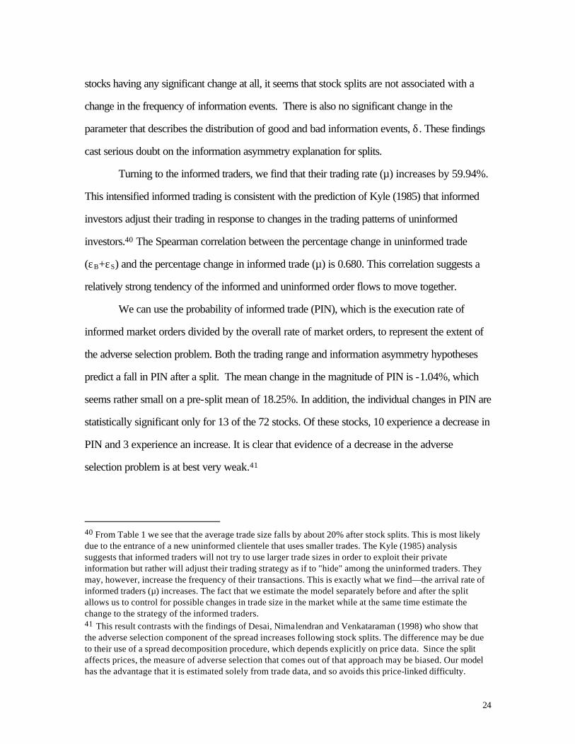
stocks having any significant change at all, it seems that stock splits are not associated with a

change in the frequency of information events. There is also no significant change in the

parameter that describes the distribution of good and bad information events, δ. These findings

cast serious doubt on the information asymmetry explanation for splits.

Turning to the informed traders, we find that their trading rate (µ) increases by 59.94%.

This intensified informed trading is consistent with the prediction of Kyle (1985) that informed

investors adjust their trading in response to changes in the trading patterns of uninformed

investors.40 The Spearman correlation between the percentage change in uninformed trade

(εB+εS) and the percentage change in informed trade (µ) is 0.680. This correlation suggests a

relatively strong tendency of the informed and uninformed order flows to move together.

We can use the probability of informed trade (PIN), which is the execution rate of

informed market orders divided by the overall rate of market orders, to represent the extent of

the adverse selection problem. Both the trading range and information asymmetry hypotheses

predict a fall in PIN after a split. The mean change in the magnitude of PIN is -1.04%, which

seems rather small on a pre-split mean of 18.25%. In addition, the individual changes in PIN are

statistically significant only for 13 of the 72 stocks. Of these stocks, 10 experience a decrease in

PIN and 3 experience an increase. It is clear that evidence of a decrease in the adverse

selection problem is at best very weak.41

40 From Table 1 we see that the average trade size falls by about 20% after stock splits. This is most likely due to the entrance of a new uninformed clientele that uses smaller trades. The Kyle (1985) analysis suggests that informed traders will not try to use larger trade sizes in order to exploit their private information but rather will adjust their trading strategy as if to "hide" among the uninformed traders. They may, however, increase the frequency of their transactions. This is exactly what we find—the arrival rate of informed traders (µ) increases. The fact that we estimate the model separately before and after the split allows us to control for possible changes in trade size in the market while at the same time estimate the change to the strategy of the informed traders. 41 This result contrasts with the findings of Desai, Nimalendran and Venkataraman (1998) who show that the adverse selection component of the spread increases following stock splits. The difference may be due to their use of a spread decomposition procedure, which depends explicitly on price data. Since the split affects prices, the measure of adverse selection that comes out of that approach may be biased. Our model has the advantage that it is estimated solely from trade data, and so avoids this price-linked difficulty.

25

Of related interest is the impact of a split on the cost of trading as measured by the

opening theoretical spread, STH. Both the trading range and informational asymmetry

hypotheses predict a decrease in STH, while the optimal tick size hypothesis predicts an

increase. As shown in equation (3), calculating STH involves both our estimated trade

parameters and the standard deviation of changes in the value of the stock, σV .42 Turning to

the volatility calculation, we find that the increase in volatility noted in the literature holds true for

our sample as well. The mean standard deviation of the daily open-to-close percentage change

in price increases from 1.44% in the pre-split period to 2.04% in the post-split period. In other

words, even when private information flow does not increase (no significant change in α), the

split increases the volatility of stocks by increasing the dispersion of their true values. As a result,

the mean percentage change in the theoretical spread measure, STH, is 42.66%. Other

researchers, noting the increase in spreads, have attributed this to greater adverse selection after

splits. Our model-based analysis shows that this inference is incorrect and that the reason for the

wider spreads is the increase in volatility.

It is interesting to compare the estimated theoretical spread with the true percentage

spread in the market.43 Such a comparison provides a simple, yet effective, check on the

reasonableness of our empirical estimates. Because no quote information is used in the

estimation of the theoretical spread, if the predicted spread is highly correlated with the actual

spread then we can attach more confidence to the predictions arising from our model. The mean

42 While our maximum likelihood procedure does not provide estimates of the true value process (V and V ), we can use market price information to construct an empirical proxy for σV . As a proxy for the

standard deviation of daily percentage changes in the value of the stock we use the standard deviation of the percentage difference between the daily closing price and the daily opening price. The results are unchanged when we repeat the analysis with the midpoints of the opening and closing quotes instead of prices. 43 Since quotes in our model are set by the market maker such that they reflect the adverse selection problem, we want to make sure that the spreads we use from the opening quotes are indeed set by the NYSE specialist. In other words, since a quote on the NYSE can be set by limit orders that were not monitored closely by those who submitted them, it need not reflect current information. Hence, we use the limit order algorithm to identify all the quotes that belong to limit orders (i.e., all the quotes that resulted in subsequent trades being categorized as limit order executions). We then calculate the opening percentage spread using the first quote of the day that is not identified as a limit order quote.

26

percentage changes in the actual opening spread, S0, and the theoretical opening spread, STH,

are 49.48% and 42.66%, respectively. While not exact, the model does a good job of

predicting actual spreads.44 The Spearman correlation between the theoretical and actual

opening percentage spreads is 0.612 in the pre-split period and 0.585 in the post-split period.

We find this relatively high correlation encouraging as it testifies to a good “fit” between our

model and the actual trading environment.

These spread results provide a partial estimate of trading costs, but to determine the

effects of stock splits on the overall cost of trading we need a measure that accounts for limit

order usage. We are specifically interested in the cost incurred by the uninformed population

since it is hard to justify stock splits on the grounds of making the privately informed population

better off.45 In a market where uninformed traders use both market and limit orders, the cost of

trading depends on the relative usage of the two types of orders. This is because when an

uninformed limit order executes against an uninformed market order, the aggregate trading cost

to the uninformed population is zero. Only when an uninformed trader’s market order executes

against the specialist or his limit order executes against an informed trader do uninformed

investors as a group incur an execution cost. Therefore, to evaluate the cost to the population of

uninformed traders we need to consider the cost of net uninformed trades (i.e., trades that were

not executed against other uninformed traders).46

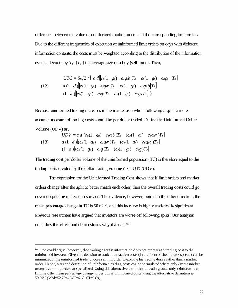
Our model provides the framework necessary to determine this cost. We define the

Uninformed Trading Cost (UTC) as half the percentage spread times the absolute value of the

44 Actual spreads are affected by factors such as tick size rules and continuity requirements, which naturally are not incorporated in our model. Nonetheless, the closeness of the actual and theoretical spreads suggests that the model does incorporate the major factors influencing spreads. 45 One could claim that a decrease in the costs incurred by informed traders might intensify costly private information gathering and therefore bring hidden firm value to the market. In this “version” of the information asymmetry story, prices adjust to information only gradually (in contrast to the revelation of public information). Hence, this has the disadvantage that markets will not be as (informationally) efficient as they could be if the private information is revealed publicly. Furthermore, this story does not help with the problem of signal credibility, since if the information is credible enough to be purchased by some traders, it should in general be credible enough for the public. 46 Note that since we are using data on limit order execution, we cannot measure the cost incurred by an uninformed trader who submits a limit order that fails to execute.

27

difference between the value of uninformed market orders and the corresponding limit orders.

Due to the different frequencies of execution of uninformed limit orders on days with different

information contents, the costs must be weighted according to the distribution of the information

events. Denote by TB (TS ) the average size of a buy (sell) order. Then,

(12)

{ [ ][ ]

[ ] }SBBSSBSSBB

SBBSSBSSBB

SBBSSBSSBBO

TT

TT

TTSTC

γεγεγεγεα

βγεγεργεγεδα

ργεγεβγεγεαδ

−−+−−−

+−−+−−−

+−−+−−=

)1()1()1(

)1()1()1(

)1()1(*2U

Because uninformed trading increases in the market as a whole following a split, a more

accurate measure of trading costs should be per dollar traded. Define the Uninformed Dollar

Volume (UDV) as,

(13) [ ]

[ ][ ]SBSSBSBB

SBBSSBSSBB

SBBSSBSSBB

TTTT

TTUDV

))1(())1(()1())1(())1(()1(

))1(())1((

γεγεγεγεαβγεγεργεγεδα

ργεγεβγεγεαδ

+−++−−++−++−−

++−++−=

The trading cost per dollar volume of the uninformed population (TC) is therefore equal to the

trading costs divided by the dollar trading volume (TC=UTC/UDV).

The expression for the Uninformed Trading Cost shows that if limit orders and market

orders change after the split to better match each other, then the overall trading costs could go

down despite the increase in spreads. The evidence, however, points in the other direction: the

mean percentage change in TC is 50.62%, and this increase is highly statistically significant.

Previous researchers have argued that investors are worse off following splits. Our analysis

quantifies this effect and demonstrates why it arises. 47

47 One could argue, however, that trading against information does not represent a trading cost to the uninformed investor. Given his decision to trade, transaction costs (in the form of the bid-ask spread) can be minimized if the uninformed trader chooses a limit order to execute his trading desire rather than a market order. Hence, a second definition of uninformed trading costs can be formulated where only excess market orders over limit orders are penalized. Using this alternative definition of trading costs only reinforces our findings: the mean percentage change in per dollar uninformed costs using the alternative definition is 59.90% (Med=52.75%, WT=6.60, ST=5.89).

28

IV. Discussion and Conclusions

In this research we have investigated the effects of stock splits on the trading in a firm’s

shares. By estimating the parameters of a market microstructure sequential trade model, we

were able to look at changes in the trading strategies of investors and in the information

environment of stocks. These changes, in turn, can be linked back to the hypotheses on why

firms split their shares. Using a structural model to extract from trade data information about

unobservable attributes such as uninformed trading, the frequency of information events, and

adverse selection provides us with a set of tools different from those used to evaluate

hypotheses on stock splits in the extant literature. Instead of using separate tests and proxies to

assess the merits of each of the hypotheses, the model enabled us to obtain an integrated set of

results with which to view all the hypotheses put forward in the literature as reasons for stock

splits. This internal consistency also allowed us to demonstrate how an increase in trading costs

can take place concurrently with an increase in uninformed trading and a more aggressive use of

limit orders.

Our results are mildly supportive of the trading range hypothesis. There is an increase in

the number of uninformed trades and a slight shift of uninformed buyers to execute their trades

by using market orders, in-line with their being more “eager” to enter the market for the stock.

This evidence is consistent with the entry of a new clientele. The increase in uninformed trading,

however, is accompanied by an increase in informed trading, and so the extent of the adverse

selection problem is not materially reduced. Increases in volatility without a substantial decrease

in adverse selection cause our spread measure to increase, and the end result is worsened

liquidity. While these results are inconsistent with the enhanced liquidity explanation of the

trading range hypothesis, they are still consistent with the trading range idea. The new clientele

may be willing to trade a stock with a higher bid-ask spread if they gain something else by

adding the stock to their portfolios (e.g., increased diversification of their holdings).

As for the information asymmetry hypothesis, the parameter estimates suggest that the

information environment of stocks does not change systematically after stock splits. The

29

increase in informed trading after the split is also difficult to reconcile with a reduction in

information asymmetry. While we report a slight decrease in the probability of informed trade, it

is too small to offset the increased cost incurred by traders due to the increase in volatility. This

increase in trading costs is inconsistent with an explanation of stock splits that implies a

reduction in adverse selection costs.

Our findings can still be viewed as consistent with a simple signaling story. If the

information revealed by the split was not known to privately informed traders (but perhaps only

to insiders who are restricted from trading), then it may be plausible that the split would not

change the structure of private information that we estimate. Furthermore, we are using only

trade data for our estimation, and the adjustment of prices to public information need not be

accompanied by trading. On the other hand, this simple signaling story does not explain why

many new traders would buy the stock after the split. If the split benefits only existing

shareholders, there should be no special incentive for a new clientele to enter.

The optimal tick size hypothesis would predict the increase in the intensity of limit order

trading that we have found, but the rest of our results seem inconsistent with this explanation.

The increase in limit order trading is not sufficient to compensate the uninformed population for

the increase in the bid-ask spread and the more intense usage of market buy orders. These

market orders face larger bid-ask spreads after the split, with the end result being that the

uninformed population suffers from an increase in its overall trading cost. In addition, the basic

intuition of the optimal tick size hypothesis is that the increased tick size after stock splits

encourages liquidity provision by inhibiting "front running." Hence, uninformed traders should be

able to decrease the monitoring of their limit orders after a split, which will result in fewer

cancelled orders. We, on the other hand, find that the execution rate of limit orders on days in

which informed traders (and prices) move against them decreases, evidence that is consistent

with an increase in limit order cancellation.

Our results suggest that stock splits are not neutral events for a security. Both changes

in the composition of the order flow and in the cost of trading accompany the decision to split.

30

In general, these changes do not enhance the overall transactional efficiency of a stock. Splitting

shares, however, does provide companies with a way to influence their ownership. If product

demand is linked to ownership, then attracting a particular clientele may enhance long-run

profitability even if it has short-run detrimental effects on liquidity.48 Such effects are beyond

our microstructure-based analysis here, but they may constitute a fruitful direction for future

research.

48 For example, companies like McDonalds encourage small ownership holdings by facilitating transfers of single shares of the stock between parents (or other adults) and children. This could be consistent with developing a new generation of customers whose loyalty is enhanced by their ownership claim.

31

References

Angel, J.J. "Tick Size, Share Price and Stock Splits." Journal of Finance, 52 (1997), 655-

681.

Angel, J.J., and R.M. Brooks, and P.G. Mathew. "When-Issued Shares, Small Traders, and

the Variance of Returns Around Stock Splits." working paper, (1997).

Anshuman, V.R., and A. Kalay. “Market Making with Discrete Prices." Review of Financial

Studies, 11 (1998), 81-109.

Arnold, T.M., and M.L. Lipson. "Tick Size and Limit Order Execution: An Examination of

Stock Splits." working paper, University of Georgia, (1997).

Barker, C.A. "Effective Stock Splits." Harvard Business Review, 34 (1956), 101-106.

Baruch, S. "Who Benefits from an Open Limit-Order Book?" working paper, (1997).

Blume, M.E., and M.A. Goldstein. "Quotes, Order Flow, and Price Discovery." Journal of

Finance, 52 (1997), 221-244.

Brennan, M.J., and T. Copeland. "Stock Splits, Stock Prices, and Transactions Costs."

Journal of Financial Economics, 22 (1988), 83-101.

Brennan, M.J., and P. Hughes. "Stock Prices and the Supply of Information." Journal of

Finance, 46 (1991), 1665-92.

Chakravarty, S., and C.W. Holden. "An Integrated Model of Market and Limit Orders."

Journal of Financial Intermediation, 4 (1995), 213-241.

Conrad, J.S., and R.M. Conroy. "Market Microstructure and the Ex-date Return." Journal of

Finance, 49 (1994), 1507-19.

32

Conroy, R.M., R.S. Harris, and B.A. Benet. "The Effects of Stock Splits on Bid-Ask Spreads."

Journal of Finance, 45 (1990), 1285-1295.

Copeland, T.E. "Liquidity Changes Following Stock Splits." Journal of Finance, 34 (1979),

115-141.

Desai, A.S., and M. Nimalendran, and S. Venkataraman. "Changes in Trading Activity

Following Stock Splits and Their Effect on Volatility and the Adverse Information

Component of the Bid-Ask Spread." Journal of Financial Research, 21 (1998), 159-

183.

Diamond, D.W., and R.E. Verrecchia. "Constraints on Short-Selling and Asset Price

Adjustment to Private Information." Journal of Financial Economics, 18 (1987), 277-

311.

Dravid, A. "A Note on the Behavior of Stock Returns Around Ex-Dates of Stock

Distributions." Journal of Finance, 42 (1987), 163-168.

Dubofsky, D.A. "Volatility Increases Subsequent to NYSE and AMEX Stock Splits." Journal

of Finance, 46 (1991), 421-31.

Dubofsky, D.A., and D.W. French. "Share Price Level and Risk: Implications for Financial

Management." Managerial Finance, 14 (1988), 6-16.

Easley, D., and M. O'Hara. "Price, Trade Size, and Information in Securities Markets." Journal

of Financial Economics, 19 (1987), 193-212.

Easley, D., N.M. Kiefer, and M. O'Hara. “Cream-Skimming or Profit-Sharing? The Curious

Role of Purchased Order Flow.” Journal of Finance, 51 (1996), 811-833.

33

Easley, D., N.M. Kiefer, and M. O'Hara. "One Day in the Life of a Very Common Stock.”

Review of Financial Studies, 10 (1997a), 805-835.

Easley, D., N.M. Kiefer, and M. O'Hara. “The Information Content of the Trading Process.”

Journal of Empirical Finance, 4 (1997b), 159-186.

Easley, D., N.M. Kiefer, M. O'Hara, and J.B. Paperman. "Liquidity, Information, and

Infrequently Traded Stocks." Journal of Finance, 51 (1996), 1405-1436.

Easley, D., M. O'Hara, and J.B. Paperman. “Financial Analysts and Information-Based Trade."

Journal of Financial Markets, 1 (1998), 175-202.

Glosten, L.R. "Is the Electronic Open Limit Order Book Inevitable?" Journal of Finance, 49

(1994), 1127-1161.

Glosten, L.R., and P. Milgrom. "Bid, Ask and Transaction Prices in a Specialist Market with

Heterogeneously Informed Traders." Journal of Financial Economics, 14 (1985), 71-

100.

Goldberger, A.S. A Course in Econometrics, Harvard University Press, Cambridge (1991).

Gray, S., Smith, T. and R. E. Whaley. “Stock Splits: Implications for Models of the Bid/Ask

Spread.” Working Paper, University of New South Wales, (1996).

Greene, J.T. "The Impact of Limit Order Executions on Trading Costs in NYSE Stocks: An

Empirical Examination." working paper, University of Georgia, (1997).

Grinblatt, M. Masulis, R. and S. Titman. “The Valuation Effects of Stock Splits and Stock

Dividends.” Journal of Financial Economics, 13 (1984), 461-490.

Harris, L. "Does a Large Minimum Price Variation Encourage Order Exposure?" working

paper, University of Southern California, (1996).

34

Harris, L. "Optimal Dynamic Order Submission Strategies in Some Stylized Trading Problems,"

Financial Markets, Institutions & Instruments, (1997).

Hasbrouck, J. "One Security, Many Markets: Determining the Contributions to Price

Discovery." Journal of Finance, 50 (1995), 1175-99.

Ikeberry, D.L., G. Rankine, and E. K. Stice. “What do Stock Splits Really Signal?”, Journal

of Financial and Quantitative Analysis, 31 (1996), 357-375.

Koski, J.L. "Measurement Effects and the Variance of Returns After Stock Splits and Stock

Dividends." Review of Financial Studies, 11 (1998), 143-162.

Kryzanowski, L., and H. Zhang. "Trading Patterns of Small and Large Traders Around Stock

Split Ex-Dates." Journal of Financial Research, 19 (1996), 75-91.

Kyle, A.S. "Continuous Auctions and Insider Trading." Econometrica, 53 (1985), 1315-36.

Lakonishok, J., and B. Lev. "Stock Splits and Stock Dividends: Why, Who, and When."

Journal of Finance, 42 (1987), 913-932.

Lamoureux, C.G., and P. Poon. "The Market Reaction to Stock Splits." Journal of Finance,

42 (1987), 1347-70.

Lee, C.M.C., and M.J. Ready. "Inferring Trade Direction from Intraday Data." Journal of

Finance, 4 (1991), 733-746.

Lipson, M.L. "Stock Splits, Liquidity, and Limit Orders." working paper, University of Georgia,

(1999).

Macey, R.M., and M. O'Hara. "The Law and Economics of Best Execution." Journal of

Financial Intermediation, 6 (1997), 188-223.

35

Madhavan, A., M. Richardson, and M. Roomans. "Why Do Security Prices Change? A

Transaction-Level Analysis of NYSE Stocks." Review of Financial Studies, 10 (1997),

1035-64.

Maloney, M.T., and J.H. Mulherin. "The Effects of Splitting on the Ex: A Microstructure

Reconciliation." Financial Management, 21 (1992), 44-59.

McNichols, M., and A. Dravid. "Stock Dividends, Stock Splits, and Signaling." Journal of

Finance, 45 (1990), 857-879.

Moore, P. G. "Nonparametric Statistics: Runs." in W. J. Kruskal and J. Tanur (eds.),

International Encyclopedia of Statistics, Free Press, New York (1978), pp. 655-661.

Muscarella, C.J., and M.R. Vetsuypens. "Stock Splits: Signaling or Liquidity? The Case of

ADR 'Solo-Splits'." Journal of Financial Economics, 42 (1996), 3-26.

NYSE, Fact Book for the Year 1995.

Ohlson, J.A., and S.H. Penman. "Volatility Increases Subsequent to Stock Splits: An Empirical

Aberration." Journal of Financial Economics, 14 (1985), 251-266.

Powell, G.E., and H.K. Baker. "The Effects of Stock Splits on the Ownership Mix of a Firm."

Review of Financial Economics, 3 (1993/1994), 70-88.

Rock, K. "The Specialist's Order Book and Price Anomalies." working paper, Harvard

University, (1990).

Saar, G. "Price Impact Asymmetry of Block Trades: An Institutional Trading Explanation."

working paper, Stern School of Business, New York University, (1999).

Schultz, P. "Stock Splits, Tick Size, and Sponsorship." Journal of Finance, 55 (2000), 429-

50.

36

Sheikh, A.M. "Stock Splits, Volatility Increases, and Implied Volatilities." Journal of Finance,

44 (1989), 1361-72.

Stovall, R.H. "Stock Split Candidates." Financial World, 164 (1995), 86.

37

Table 1

Summary Statistics This table contains summary statistics for the firms used in the study. The sample consists of 72 firms. To be included in the sample, a firm had to be lis ted on the NYSE and have a 2-to-1 stock split in 1995. The pre-split period consists of 45 days and ends 20 days before the announcement date of the split. The post-split period consists of 45 days and starts 20 days after the ex-date of the split. Panel A provides descriptive statistics on market capitalization and trading. The variables are calculated for each stock separately before the cross sectional sample statistics are computed. Market capitalization of firms in the sample is taken from the CRSP database and is defined as their value at the end of 1995. Data on the average size of buy and sell orders and the daily number of trades is taken from the TAQ database. Only NYSE trades are considered. The classification into buy and sell orders is done using the Lee and Ready (1991) algorithm. Panel B provides descriptive statistics on prices and spreads. The variables are calculated for each stock separately before the cross sectional sample statistics are computed. The opening spread is the difference between the bid and the ask of the opening quote on the NYSE. Proportional spreads are spreads divided by the mid-quote.

Panel A:

Average Daily Number

of Trades

Average Size

of Buy Orders

Average Size

of Sell Orders

Market

Capitalization

(millions) Pre-Split Post-Split Pre-Split Post-Split Pre-Split Post-Split

Mean $5,847 97.52 158.77 $81,480 $64,658 $82,553 $77,955

Std. Dev. $9,366 109.47 198.82 $50,797 $44,295 $46,639 $47,378

100% (Max) $43,216 551.84 1155.29 $226,879 $202,282 $206,889 $204,982

75% (Q3) $6,753 126.17 185.80 $110,757 $87,384 $112,680 $105,589

50% (Med) $1,947 48.89 83.73 $75,894 $56,978 $81,971 $72,548

25% (Q1) $1,028 27.74 34.67 $39,325 $32,111 $43,498 $35,673

0% (Min) $245 6.02 7.56 $14,908 $10,891 $15,111 $13,426

Panel B: Average Closing Price Average Dollar Opening

Spread

Average Percentage

Opening Spread

Pre-Split Post-Split Pre-Split Post-Split Pre-Split Post-Split

Mean $54.90 $34.28 $0.326 $0.289 0.68% 0.99%

Std. Dev. $19.99 $14.72 $0.072 $0.049 0.29% 0.39%

100% (Max) $127.86 $82.06 $0.708 $0.394 1.71% 2.14%

75% (Q3) $68.03 $41.97 $0.358 $0.329 0.85% 1.31%

50% (Med) $47.67 $32.29 $0.321 $0.288 0.67% 0.97%

25% (Q1) $40.59 $23.57 $0.281 $0.249 0.44% 0.64%

0% (Min) $21.15 $11.67 $0.255 $0.189 0.20% 0.31%

38

Table 2 Implications of Hypotheses about Stock Splits

This table presents the implications of the different hypotheses about stock splits for the parameters of the trading model. The notation "+" ("-") should be read as a predicted increase (decrease) in the parameter. An empty cell means that the hypothesis does not have a clear implication concerning the parameter, and "+/0" means that two versions of the same hypothesis have different implications (increase or no change). εB (εS) is the rate at which uninformed buy (sell) orders are executed and γB (γS) is the fraction of uninformed limit buy (sell) orders. µ is the arrival rate of informed traders, α is the probability of an information event and δ is the probability of bad information. On days with information events, β is the rate at which limit orders are executed when the orders are in the same direction as the information and ρ is the rate at which limit orders are executed when the orders are in the opposite direction to the information (relative to the rate on no information days). PIN is a function of the parameters that represents the probability of informed trade (equation (11)). STH is the theoretical opening spread expression that comes out of the model (equation (5)). TC is a measure of the total trading costs of the population of uninformed traders that is developed in Section III.

ε B ε S Bγ Sγ µ α δ β ρ PIN STH TC

Trading Range + + - - - -

Information Asymmetry - - - -

Optimal Tick Size +/0 +/0 + + + + -

39

Table 3 Results

εB (εS) is the rate at which uninformed buy (sell) orders are executed and γB (γS) is the fraction of uninformed limit buy (sell) orders. γBεB (γSεS) is therefore the rate at which uninformed limit orders are executed on no information days. On days with information events, β is the rate at which limit orders are executed when the orders are in the same direction as the information and ρ is the rate at which limit orders are executed when the orders are in the opposite direction to the information (relative to the rate on no information days). α is the probability of an information event occurring, δ (1-δ) is the probability that an information event is bad (good), and µ is the arrival rate of informed traders. PIN is a function of the parameters that represents the probability of informed trade (equation (11)). STD is the standard deviation of daily percentage opening to closing price changes. STH is the theoretical opening spread expression that comes out of the model (equation (5)). TC is a measure of the overall trading costs (per dollar) of the population of uninformed traders that is developed in Section III. Panel A presents the mean and the median of the percentage change (or magnitude change where appropriate) in the parameters. The Wilcoxon signed-rank statistic and the Sign statistic are calculated using the standard normal approximation. The critical values for a two-sided alternative are 1.96 and 1.64 for 5% and 10% significance levels, respectively. The 5% significance level is used in reporting the results of the χ2 tests. Panel B presents Pearson and Spearman correlations (with asymptotic standard errors). The notation "%∆" represents percentage change. S0 is the opening percentage spread (dollar spread over the midquote). Panel A:

Percentage Change Non-Parametric Tests Significant χ2 Tests

Mean Median Wilcoxon Sign Increases Decreases

εB 66.71% 61.40% 7.16 7.54 64 2

εS 58.70% 47.64% 6.74 5.66 59 3

µ

59.94% 37.26% 4.39 2.83 39 12

β -0.23% -3.12% -0.66 -0.94 11 12

ρ -6.89% -6.43% -2.70 -3.06 6 18

STH 42.66% 26.67% 4.33 3.94

γBεB 86.83% 53.20% 6.63 5.85

γSεS 77.24% 59.58% 7.00 7.31

TC 50.62% 42.68% 6.35 5.89

Magnitude Change

α 1.83% 4.07% 0.63 0.71 10 6

δ -0.05% -2.25% -0.28 -0.47 7 10

γB -1.18% -1.61% -1.75 -1.65 15 25

γS 2.59% 2.59% 2.92 2.59 27 12

PIN -1.04% -1.04% -2.03 -2.36 3 10

STD 0.60% 0.54% 6.64 7.54

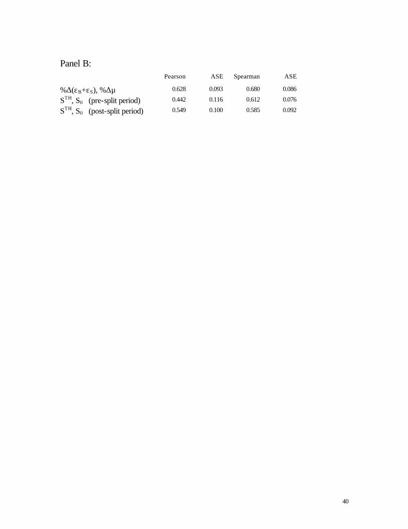
40

Panel B: Pearson ASE Spearman ASE

%∆(εB+εS), %∆µ 0.628 0.093 0.680 0.086

STH, S0 (pre-split period) 0.442 0.116 0.612 0.076

STH, S0 (post-split period) 0.549 0.100 0.585 0.092

41

Figure 1 Probability Tree of the Trading Model

This figure presents the probabilities associated with the events and outcomes of the trading model. To the left of the gray line are events that take place once a day before the beginning of trading. An information event occurs with probability α, and if it occurs, the information is bad (good) with probability δ (1-δ). To the right of the gray line are events that take place during the trading day. εB (εS) is the rate at which uninformed buy (sell) orders are executed and γB (γS) is the fraction of uninformed limit buy (sell) orders. On days with information events, β is the rate at which limit orders are executed when the orders are in the same direction as the information and ρ is the rate at which limit orders are executed when the orders are in the opposite direction to the information (relative to the rate on no information days). µ is the arrival rate of informed traders.