HAL Id: hal-00766012https://hal.archives-ouvertes.fr/hal-00766012

Submitted on 17 Dec 2012

HAL is a multi-disciplinary open accessarchive for the deposit and dissemination of sci-entific research documents, whether they are pub-lished or not. The documents may come fromteaching and research institutions in France orabroad, or from public or private research centers.

L’archive ouverte pluridisciplinaire HAL, estdestinée au dépôt et à la diffusion de documentsscientifiques de niveau recherche, publiés ou non,émanant des établissements d’enseignement et derecherche français ou étrangers, des laboratoirespublics ou privés.

The Metallicity Evolution of Star-Forming Galaxies fromRedshift 0 to 3: Combining Magnitude Limited Survey

with Gravitational LensingT.-T. Yuan, L. J. Kewley, J. Richard

To cite this version:T.-T. Yuan, L. J. Kewley, J. Richard. The Metallicity Evolution of Star-Forming Galaxies from Red-shift 0 to 3: Combining Magnitude Limited Survey with Gravitational Lensing. Applied Organometal-lic Chemistry, Wiley-Blackwell, 2012, 1211, pp.6423. hal-00766012

arX

iv:1

211.

6423

v1 [

astr

o-ph

.CO

] 27

Nov

201

2DRAFT VERSIONNOVEMBER 28, 2012Preprint typeset using LATEX style emulateapj v. 5/2/11

THE METALLICITY EVOLUTION OF STAR-FORMING GALAXIES FROM REDSHIFT 0 TO 3: COMBININGMAGNITUDE LIMITED SURVEY WITH GRAVITATIONAL LENSING

T.-T. YUAN1,2, L. J. KEWLEY1,2,3, J. RICHARD4

Draft version November 28, 2012

ABSTRACTWe present a comprehensive observational study of the gas phase metallicity of star-forming galaxies from

z ∼ 0 → 3. We combine our new sample of gravitationally lensed galaxies with existing lensed and non-lensed samples to conduct a large investigation into the mass-metallicity (MZ) relation atz > 1. We apply aself-consistent metallicity calibration scheme to investigate the metallicity evolution of star-forming galaxiesas a function of redshift. The lensing magnification ensuresthat our sample spans an unprecedented range ofstellar mass (3× 107−6×1010 M⊙). We find that at the median redshift ofz = 2.07, the median metallicityof the lensed sample is 0.35 dex lower than the local SDSS star-forming galaxies and 0.18 dex lower than thez ∼ 0.8 DEEP2 galaxies. We also present thez ∼ 2 MZ relation using 19 lensed galaxies. A more rapidevolution is seen betweenz ∼ 1 → 3 thanz ∼ 0 → 1 for the high-mass galaxies (109.5 M⊙ <M⋆ <1011

M⊙), with almost twice as much enrichment betweenz ∼ 1 → 3 than betweenz ∼ 1 → 0. We comparethis evolution with the most recent cosmological hydrodynamic simulations with momentum driven winds. Wefind that the model metallicity is consistent with the observed metallicity within the observational error forthe low mass bins. However, for higher masses, the model over-predicts the metallicity at all redshifts. Theover-prediction is most significant in the highest mass bin of 1010−11 M⊙.Subject headings:galaxies: abundances — galaxies: evolution — galaxies: high-redshift — gravitational

lensing: strong

1. INTRODUCTION

Soon after the pristine clouds of primordial gas collapsedto assemble a protogalaxy, star formation ensued, leading tothe production of heavy elements (metals). Metals were syn-thesized exclusively in stars, and were ejected into the inter-stellar medium (ISM) through stellar winds or supernovae ex-plosions. Tracing the heavy element abundance (metallicity)in star-forming galaxies provides a “fossil record” of galaxyformation and evolution.

When considered as a closed system, the metal content of agalaxy is directly related to the yield and gas fraction (Searle& Sargent 1972; Pagel & Patchett 1975; Pagel & Edmunds1981; Edmunds 1990). In reality, a galaxy interacts withits surrounding intergalactic medium (IGM), hence both theoverall and local metallicity distribution of a galaxy is mod-ified by feedback processes such as galactic winds, inflows,and gas accretions (e.g., Lacey & Fall 1985; Edmunds &Greenhow 1995; Koppen & Edmunds 1999; Dalcanton 2007).Therefore, observations of the chemical abundances in galax-ies offer crucial constraints on the star formation historyandvarious mechanisms responsible for galactic inflows and out-flows.

The well-known correlation between galaxy mass (lumi-nosity) and metallicity was first proposed by Lequeux et al.(1979). Subsequent studies confirmed the existence of theluminosity-metallicity (LZ) relation (e.g., Rubin et al. 1984;Skillman et al. 1989; Zaritsky et al. 1994; Garnett 2002).Luminosity was used as a proxy for stellar mass in these

1 Institute for Astronomy, University of Hawaii, 2680 Woodlawn Drive,Honolulu, HI 96822

2 Research School of Astronomy and Astrophysics, The Australian Na-tional University, Cotter Road, Weston Creek, ACT 2611

3 ARC Future Fellow4 CRAL, Observatoire de Lyon, Universite Lyon 1, 9 avenue Charles

Andre, 69561 Saint Genis Laval Cedex, France

studies as luminosity is a direct observable. Aided by newsophisticated stellar population models, stellar mass canberobustly calculated and a tighter correlation is found in themass-metallicity (MZ) relation. Tremonti et al. (2004) haveestablished the MZ relation for local star-forming galaxiesbased on∼ 5×105 Sloan Digital Sky Survey (SDSS) galax-ies. At intermediate redshifts (0.4 < z < 1), the MZ relationhas also been observed for a large number of galaxies (>100)(e.g., Savaglio et al. 2005; Cowie & Barger 2008; Lamareilleet al. 2009). Zahid et al. (2011) derived the MZ relation for∼103 galaxies from the Deep Extragalactic Evolutionary Probe2 (DEEP2) survey, validating the MZ relation on a statisticallysignificant level atz ∼ 0.8.

Current cosmological hydrodynamic simulations and semi-analytical models can predict the metallicity history of galax-ies on a cosmic timescale (Nagamine et al. 2001; De Luciaet al. 2004; Bertone et al. 2007; Brooks et al. 2007; Dave &Oppenheimer 2007; Dave et al. 2011a,b). These models showthat the shape of the MZ relation is particularly sensitive to theadopted feedback mechanisms. The cosmological hydrody-namic simulations with momentum-driven winds models pro-vide better match with observations than energy-driven windmodels (Oppenheimer & Dave 2008; Finlator & Dave 2008;Dave et al. 2011a). However, these models have not beentested thoroughly in observations, especially at high redshifts(z > 1), where the MZ relation is still largely uncertain.

As we move to higher redshifts, selection effects and smallnumber statistics haunt observational metallicity history stud-ies. The difficulty becomes more severe in the so-called “red-shift desert” (1 . z . 3), where the metallicity sensitive op-tical emission lines have shifted to the sky-background dom-inated near infrared (NIR). Ironically, this redshift range har-bors the richest information about galaxy evolution. It is dur-ing this redshift period (∼ 2−6 Gyrs after the Big Bang) thatthe first massive structures condensed; the star formation rate

2

(SFR), major merger activity, and black hole accretion ratepeaked; much of today’s stellar mass was assembled, andheavy elements were produced (Fan et al. 2001; Dickinsonet al. 2003; Chapman et al. 2005; Hopkins & Beacom 2006;Grazian et al. 2007; Conselice et al. 2007; Reddy et al. 2008).It is therefore of crucial importance to explore NIR spectraforgalaxies in this redshift range.

Many spectroscopic redshift surveys have been carried outto study star-forming galaxies atz >1 in recent years (e.g.,Steidel et al. 2004; Law et al. 2009). However, due to thelow efficiency in the NIR, those spectroscopic surveys al-most inevitably have to rely on color-selection criteria and thebiases in UV-selected galaxies tend to select the most mas-sive and less dusty systems (e.g., Capak et al. 2004; Steidelet al. 2004; Reddy et al. 2006). Space telescopes can observemuch deeper in the NIR and are able to probe a wider massrange. For example, the narrow-band Hα surveys based onthe new WFC3 camera aboard the Hubble Space Telescope(HST) have located hundreds of Hα emitters up to z = 2.23,finding much fainter systems than observed from the ground(Sobral et al. 2009). However, the low-resolution spectra fromthe narrow band filters forbid derivations of physical proper-ties such as metallicities that can only currently be acquiredfrom ground-based spectral analysis.

Thanks to the advent of long-slit/multi-slit NIR spectro-graphs on 8−10 meter class telescopes, enormous progresshas been made in the last decade to capture galaxies in theredshift desert. For chemical abundance studies, a full cov-erage of rest-frame optical spectra (4000−9000A) is usuallymandatory for the most robust diagnostic analysis. For 1.5. z . 3, the rest-frame optical spectra have shifted intothe J, H, and K bands. It remains challenging and observa-tionally expensive to obtain high signal-to-noise (S/N ) NIRspectra from the ground, especially for “typical” targets athigh-z that are less massive than conventional color-selectedgalaxies. Therefore, previous investigations into the metallic-ity properties between1 . z . 3 focused on stacked spec-tra, samples of massive luminous individual galaxies, or verysmall numbers of lower-mass galaxies (e.g., Erb et al. 2006;Forster Schreiber et al. 2006; Law et al. 2009; Erb et al. 2010;Yabe et al. 2012).

The first mass-metallicity (MZ) relation for galaxies at z∼2 was found by Erb et al. (2006) using the stacked spectraof 87 UV selected galaxies divided into 6 mass bins. Sub-sequently, mass and metallicity measurements have been re-ported for numerous individual galaxies at 1.5< z < 3(Forster Schreiber et al. 2006; Genzel et al. 2008; Hayashiet al. 2009; Law et al. 2009; Erb et al. 2010). These galaxiesare selected using broadband colors in the UV (Lyman Breaktechnique; Steidel et al. 1996, 2003) or using B, z, and K-band colors (BzK selection; Daddi et al. 2004). The Lymanbreak and BzK selection techniques favor galaxies that are lu-minous in the UV or blue and may therefore be biased againstlow luminosity (low-metallicity) galaxies, and dusty (poten-tially metal-rich) galaxies. Because of these biases, galaxiesselected in this way may not sample the full range in metal-licity at redshift z>1.

A powerful alternative method to avoid these selection ef-fects is to use strong gravitationally lensed galaxies. In thecase of galaxy cluster lensing, the total luminosity and area ofthe background sources can easily be boosted by∼ 10 − 50times, providing invaluable opportunities to obtain high S/Nspectra and probe intrinsically fainter systems within a rea-sonable amount of telescope time. In some cases, sufficient

S/N can even be obtained for spatially resolved pixels to studythe resolved metallicity of high-z galaxies (Swinbank et al.2009; Jones et al. 2010; Yuan et al. 2011; Jones et al. 2012).Before 2011, metallicities have been reported for a handfulofindividually lensed galaxies using optical emission linesat 1.5< z < 3 (Pettini et al. 2001; Lemoine-Busserolle et al. 2003;Stark et al. 2008; Quider et al. 2009; Yuan & Kewley 2009;Jones et al. 2010). Fortunately, lensed galaxy samples withmetallicity measurements have increased significantly thanksto reliable lensing mass modeling and larger dedicated spec-troscopic surveys of lensed galaxies on 8-10 meter telescopes(Richard et al. 2011; Wuyts et al. 2012; Christensen et al.2012).

In 2008, we began a spectroscopic observational survey de-signed specifically to capture metallicity sensitive linesforlensed galaxies. Taking advantage of the multi-object cryo-genic NIR spectrograph (MOIRCS) on Subaru, we targetedwell-known strong lensing galaxy clusters to obtain metallic-ities for galaxies between 0.8< z < 3. In this paper, wepresent the first metallicity measurement results from our sur-vey.

Combining our new data with existing data from the litera-ture, we present a coherent observational picture of the metal-licity history and mass-metallicity evolution of star-forminggalaxies fromz ∼ 0 to z ∼ 3. Kewley & Ellison (2008) haveshown that the metallicity offsets in the diagnostic methodscan easily exceed the intrinsic trends. It is of paramount im-portance to make sure that relative metallicities are comparedon the same metallicity calibration scale. In MZ relation stud-ies, the methods used to derive the stellar mass can also causesystematic offsets (Zahid et al. 2011). Different SED fittingcodes can yield a non-negligible mass offset, hence mimick-ing or hiding evolution in the MZ relation. In this paper, wederive the mass and metallicity of all samples using the samemethods, ensuring that the observational data are comparedina self-consistent way. We compare our observed metallicityhistory with the latest prediction from cosmological hydrody-namical simulations.

Throughout this paper we use a standardΛCDM cosmologywith H0= 70 km s−1 Mpc−1, ΩM=0.30, andΩΛ=0.70. Weuse solar oxygen abundance 12 + log(O/H)⊙=8.69 (Asplundet al. 2009).

The paper is organized as follows: Section 2 describes ourlensed sample survey and observations. Data reduction andanalysis are summarized in Section 3. Section 4 presents anoverview of all the samples we use in this study. Section 5 de-scribes the methodology of derived quantities. The metallicityevolution of star-forming galaxies with redshift is presented inSection 6. Section 7 presents the mass-metallicity relation forour lensed galaxies. Section 8 compares our results with pre-vious work in literature. Section 9 summarizes our results.Inthe Appendix, we show the morphology, slit layout, and re-duced 1D spectra for the lensed galaxies reported in our sur-vey.

2. THE LEGMS SURVEY AND OBSERVATIONS

2.1. The Lensed Emission-Line Galaxy Metallicity Survey(LEGMS)

Our survey (LEGMS) aims to obtain oxygen abundanceof lensed galaxies at 0.8<z<3. LEGMS has taken enor-mous advantage of the state-of-the-art instruments on MaunaKea. Four instruments have been utilized so far: (1) theMulti-Object InfraRed Camera and Spectrograph (MOIRCS;

3

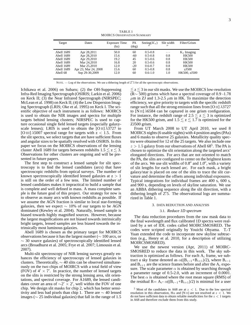
TABLE 1MOIRCS OBSERVATION SUMMARY

Target Dates Exposure Time PA Seeing(Ks) Slit width Filter/Grism(ks) (deg) ′′ ′′

Abell 1689 Apr 28,2011 50.0 60 0.5-0.8 · · · Ks ImagingAbell 1689 Apr 28,2010 15.6 -60 0.5-0.8 0.8 HK500Abell 1689 Apr 29,2010 19.2 45 0.5-0.6 0.8 HK500Abell 1689 Mar 24,2010 16.8 20 0.5-0.6 0.8 HK500Abell 1689 Mar 25,2010 12.0 -20 0.6-0.7 0.8 HK500Abell 1689 Apr 23, Mar 24, 2008 15.6 60 0.5-0.8 0.8 zJ500Abell 68 Sep 29-30,2009 12.0 60 0.6-1.0 1.0 HK500, zJ500

NOTE. — Log of the observations. We use a dithering length of 2.′′5 for all the spectroscopic observations.

Ichikawa et al. 2006) on Subaru; (2) the OH-SuppressingInfra-Red Imaging Spectrograph (OSIRIS; Larkin et al. 2006)on Keck II; (3) the Near Infrared Spectrograph (NIRSPEC;McLean et al. 1998) on Keck II; (4) the Low Dispersion Imag-ing Spectrograph (LRIS; Oke et al. 1995) on Keck I. The sci-entific objective of each instrument is as follows: MOIRCSis used to obtain the NIR images and spectra for multipletargets behind lensing clusters; NIRSPEC is used to cap-ture occasional single field lensed targets (especially galaxy-scale lenses); LRIS is used to obtain the [OII ] λ3727 to[O III ] λ5007 spectral range for targets with z< 1.5. Fromthe slit spectra, we select targets that are have sufficient fluxesand angular sizes to be spatially resolved with OSIRIS. In thispaper we focus on the MOIRCS observations of the lensingcluster Abell 1689 for targets between redshifts 1.5. z . 3.Observations for other clusters are ongoing and will be pre-sented in future papers.

The first step to construct a lensed sample for slit spec-troscopy is to find the lensed candidates (arcs) that havespectroscopic redshifts from optical surveys. The number ofknown spectroscopically identified lensed galaxies at z> 1is still on the order of a few tens. The limited number oflensed candidates makes it impractical to build a sample thatis complete and well defined in mass. A mass complete sam-ple is the future goal of this project. Our strategy for now isto observe as many arcs with known redshifts as possible. Ifwe assume the AGN fraction is similar to local star-forminggalaxies, then we expect∼ 10% of our targets to be AGNdominated (Kewley et al. 2004). Naturally, lensed sample isbiased towards highly magnified sources. However, becausethe largest magnifications are not biased towards intrinsicallybright targets, lensed samples are less biased towards the in-trinsically most luminous galaxies.

Abell 1689 is chosen as the primary target for MOIRCSobservations because it has the largest number (∼ 100 arcs, or∼ 30 source galaxies) of spectroscopically identified lensedarcs (Broadhurst et al. 2005; Frye et al. 2007; Limousin et al.2007).

Multi-slit spectroscopy of NIR lensing surveys greatly en-hances the efficiency of spectroscopy of lensed galaxies inclusters. Theoretically,∼ 40 slits can be observed simultane-ously on the two chips of MOIRCS with a total field of view(FOV) of 4′ × 7′. In practice, the number of lensed targetson the slits is restricted by the strong lensing area, slit orien-tations, and spectral coverage. For A1689, the lensed candi-dates cover an area of∼2′ × 2′, well within the FOV of onechip. We design slit masks for chip 2, which has better sensi-tivity and less bad pixels than chip 1. There are∼ 40 lensedimages (∼ 25 individual galaxies) that fall in the range of 1.5

. z. 3 in our slit masks. We use the MOIRCS low-resolution(R∼ 500) grisms which have a spectral coverage of 0.9 -1.78µm in ZJ and 1.3-2.5µm in HK. To maximize the detectionefficiency, we give priority to targets with the specific redshiftrange such that all the strong emission lines from [OII ] λ3727to [N II ] λ6584 can be captured in one grism configuration.For instance, the redshift range of 2.5. z . 3 is optimizedfor the HK500 grism, and 1.5. z . 1.7 is optimized for theZJ500 grism.

From UT March 2008 to UT April 2010, we used 8MOIRCS nights (6 usable nights) with 4 position angles (PAs)and 6 masks to observe 25 galaxies. Metallicity quality spec-tra were obtained for 12 of the 25 targets. We also include onez > 1.5 galaxy from our observations of Abell 685. The PA ischosen to optimize the slit orientation along the targeted arcs’elongated directions. For arcs that are not oriented to matchthe PA, the slits are configured to center on the brightest knotsof the arcs. We use slit widths of 0.8′′ and 1.0′′, with a varietyof slit lengths for each lensed arc. For each mask, a brightgalaxy/star is placed on one of the slits to trace the slit cur-vature and determine the offsets among individual exposures.Typical integrations for individual frames are 400 s, 600 s,and 900 s, depending on levels of skyline saturation. We usean ABBA dithering sequence along the slit direction, with adithering length of 2.′′5. The observational logs are summa-rized in Table 1.

3. DATA REDUCTION AND ANALYSIS

3.1. Reduce 1D spectrum

The data reduction procedures from the raw mask data tothe final wavelength and flux calibrated 1D spectra were real-ized by a set of IDL codes called MOIRCSMOSRED. Thecodes were scripted originally by Youichi Ohyama. T.-TYuan extended the code to incorporate new skyline subtrac-tion (e.g., Henry et al. 2010, for a description of utilizingMOIRCSMOSRED).

We use the newest version (Apr, 2011) of MOIRC-SMOSRED to reduce the data in this work. The sky sub-traction is optimized as follows. For each Ai frame, we sub-tract a sky frame denoted asα((Bi−1+Bi+1)/2), where Bi−1

and Bi+1 are the science frames before and after the Ai expo-sure. The scale parameterα is obtained by searching througha parameter range of 0.5-2.0, with an increment of 0.0001.The bestα is obtained where the root mean square (RMS) ofthe residual R= Ai- α((Bi−1+Bi+1)/2) is minimal for a user

5 Most of the candidates in A68 are atz < 1. Due to the low spectralresolution in this observation, Hα and [NII ] are not resolved atz < 1. Wedo not have sufficient data to obtain reliable metallicitiesfor thez < 1 targetsin A68 and therefore exclude them from this study.

4

defined wavelength regionλ1 andλ2. We find that this skysubtraction method yields smaller sky OH line residuals (∼20%) than conventional A-B methods. We also compare withother skyline subtraction methods in literature (Kelson 2003;Davies 2007). We find the sky residuals from our methodare comparable to those from the Kelson (2003) and Davies(2007) methods within 5% in general cases. However, incases where the emission line falls on top of a strong skyline,our method is more stable and improves the skyline residualby∼ 10% than the other two methods.

Wavelength calibration is carried out by identifying sky-lines for the ZJ grism. For the HK grism, we use argon lines tocalibrate the wavelength since only a few skylines are avail-able in the HK band. The argon-line calibrated wavelengthis then re-calibrated with the available skylines in HK to de-termine the instrumentation shifts between lamp and scienceexposures. Note that the RMS of the wavelength calibrationusing a 3rd order polynomial fitting is∼ 10-20A, correspond-ing to a systematic redshift uncertainty of 0.006.

A sample of A0 stars selected from the UKIRT photomet-ric standards were observed at similar airmass as the targets.These stars were used for both telluric absorption correctionsand flux calibrations. We use the prescriptions of Erb et al.(2003) for flux calibration. As noted in Erb et al. (2003),the absolute flux calibration in the NIR is difficult with typ-ical uncertainties of∼20%. We note that this uncertainty iseven larger for lensed samples observed in multi-slits becauseof the complicated aperture effects. The uncertainties in theflux calibration are not a concern for our metallicity analysiswhere only line ratios are involved. However, these errors area major concern for calculating SFRs. The uncertainties fromthe multi-slit aperture effects can cause the SFRs to changeby a factor of 2-3. For this reason, we refrain from any quan-titative analysis of SFRs in this work.

3.2. Line Fitting

The emission lines are fitted with Gaussian profiles. Forthe spatially unresolved spectra, the aperture used to extractthe spectrum is determined by measuring the Gaussian profileof the wavelength collapsed spectrum. Some of the lensedtargets (∼ 10%) are elongated and spatially resolved in theslit spectra, however, because of the low surface brightnessand thus very low S/N per pixel, we are unable to obtain us-able spatially resolved spectra. For those targets, we makean initial guess for the width of the spatial profile and forceaGaussian fit, then we extract the integrated spectrum using theaperture determined from the FWHM of the Gaussian profile.

For widely separated lines such as [OII ] λ3727, Hβ λ4861,single Gaussian functions are fitted with 4 free parameters:the centroid (or the redshift), the line width, the line flux,andthe continuum. The doublet [OIII ] λλ4959,5007 are initiallyfitted as a double Gaussian function with 6 free parameters:the centroids 1 and 2 , line widths 1 and 2, fluxes 1 and 2,and the continuum. In cases where the [OIII ] λ4959 line istoo weak, its centroid and line velocity width are fixed to bethe same as [OIII ] λ5007 and the flux is fixed to be 1/3 ofthe [OIII ] λ5007 line (Osterbrock 1989). A triple-Gaussianfunction is fitted simultaneously to the three adjacent emis-sion lines: [NII ] λ6548, 6583 and Hα. The centroid and ve-locity width of [N II ] λ6548, 6583 lines are constrained by thevelocity width of Hαλ6563, and the ratio of [NII ] λ6548 and[N II ] λ6583 is constrained to be the theoretical value of 1/3given in Osterbrock (1989). The line profile fitting is con-ducted using aχ2 minimization procedure which uses the in-

verse of the sky OH emission as the weighting function. TheS/N per pixel is calculated from theχ2 of the fitting. The mea-sured emission line fluxes and line ratios are listed in Table4.The final reduced 1D spectra are shown in the Appendix.

3.3. Lensing Magnification

Because the lensing magnification (µ) is not a direct func-tion of wavelength, line ratio measurements do not requirepre-knowledge of the lensing magnification. However,µ isneeded for inferring other physical properties such as the in-trinsic fluxes, masses and source morphologies. Paramet-ric models of the mass distribution in the clusters Abell 68and Abell 1689 were constructed using the Lenstool softwareLenstool6 (Kneib et al. 1993; Jullo et al. 2007). The best-fit models have been previously published in Richard et al.(2007) and Limousin et al. (2007). As detailed in Limousinet al. (2007),Lenstool uses Bayesian optimization witha Monte-Carlo Markov Chain (MCMC) sampler which pro-vides a family of best models sampling the posterior proba-bility distribution of each parameter. In particular, we use thisfamily of best models to derive the magnification and rela-tive error on magnificationµ associated to each lensed source.Typical errors onµ are∼10% for Abell 1689 and Abell 68.

3.4. Photometry

We determine the photometry for the lensed galaxies inA1689 using 4-bandHST imaging data, 1-band MOIRCSimaging data, and 2-channelSpitzerIRAC data at 3.6 and 4.5µm.

We obtained a 5,000 s image exposure for A1689 on theMOIRCS Ks filter, at a depth of 24 mag, using a scale of0.117′′ per pixel. The image was reduced using MCSREDin IRAF written by the MOIRCS supporting astronomer IchiTanaka7. The photometry is calibrated using the 2MASS starslocated in the field.

The ACS F475W, F625W, F775W, F850LP data are ob-tained from theHSTarchive. TheHSTphotometry are de-termined using SExtractor (Bertin & Arnouts 1996) with pa-rameters adjusted to detect the faint background sources. TheF775W filter is used as the detection image using a 1.′′0 aper-ture.

The IRAC data are obtained from theSpitzerarchive andare reduced and drizzled to a pixel scale of 0.′′6 pixel−1. Inorder to include the IRAC photometry, we convolved theHSTand MOIRCS images with the IRAC point spread functions(PSFs) derived from unsaturated stars. All photometric dataare measured using a 3.′′0 radius aperture. Note that we onlyconsider sources that are not contaminated by nearby brightgalaxies:∼ 70% of our sources have IRAC photometry (Ta-ble 5). Typical errors for the IRAC band photometry are 0.3mag, with uncertainties mainly from the aperture correctionand contamination of neighboring galaxies. Typical errorsforthe ACS and MOIRCS bands are 0.15 mag, with uncertaintiesmainly from the Poisson noise and absolute zero-point uncer-tainties (Wuyts et al. 2012). We refer to Richard et al. (2012,in prep) for the full catalog of the lensing magnification andphotometry of the lensed sources in Abell 1689.

4. SUPPLEMENTARY SAMPLES

In addition to our lensed targets observed in LEGMS, wealso include literature data for complementary lensed and

6 http://www.oamp.fr/cosmology/lenstool7 http://www.naoj.org/staff/ichi/MCSRED/mcsred.html

5

non-lensed samples at both local and high-z. The observa-tional data for individually measured metallicities at z> 1.5are still scarce and caution needs to be taken when using themfor comparison. The different metallicity and mass derivationmethods used in different samples can give large systematicdiscrepancies and provide misleading results. For this rea-son, we only include the literature data that have robust mea-surements and sufficient data for consistently recalculating thestellar mass and metallicities using our own methods. Thus,in general, stacked data, objects with lower/upper limits in ei-ther line ratios or masses arenot chosen. The one exceptionis the stacked data of Erb et al. (2006), as it is the most widelyused comparison sample atz ∼ 2.

The samples used in this work are:(1) The Sloan Digital Sky Survey (SDSS) sample (z ∼

0.07). We use the SDSS sample (Abazajian et al. 2009,http://www.mpa-garching.mpg.de/SDSS/DR7/) defined byZahid et al. (2011). The mass derivation method used inZahid et al. (2011) is the same as we use in this work.All SDSS metallicities are recalculated using the PP04N2method, which uses an empirical fit to the [NII ] and Hα lineratios of HII regions (Pettini & Pagel 2004).

(2) The The Deep Extragalactic Evolutionary Probe 2(DEEP2) sample (z ∼ 0.8). The DEEP2 sample (Daviset al. 2003, http://www.deep.berkeley.edu/DR3/) is definedin Zahid et al. (2011). Atz ∼ 0.8, the [NII ] and Hα linesare not available in the optical. We convert the KK04 R23

metallicity to the PP04N2 metallicity using the prescriptionsof Kewley & Ellison (2008).

(3) The UV-selected sample (z ∼ 2). We use the stackeddata of Erb et al. (2006). The metallicity diagnostic used byErb et al. (2006) is the PP04N2 method and no recalculationis needed. We offset the stellar mass scale of Erb et al. (2006)by -0.3 dex to match the mass derivation method used inthis work (Zahid et al. 2012). This offset accounts for thedifferent initial mass function (IMF) and stellar evolutionmodel parameters applied by Erb et al. (2006).

(4) The lensed sample (1< z< 3). Besides the 11 lensedgalaxies from our LEGMS survey in Abell 1689, we include1 lensed source (z =1.762) from our MOIRCS data onAbell 68 and 1 lensed spiral (z =1.49) from Yuan et al.(2011). We also include 10 lensed galaxies from Wuyts et al.(2012) and 3 lensed galaxies from Richard et al. (2011),since these 13 galaxies have [NII ] and Hα measurements,as well as photometric data for recalculating stellar masses.We require all emission lines from literature to have S/N> 3 for quantifying the metallicity of 1< z < 3 galaxies.Upper-limit metallicities are found for 6 of the lensed targetsfrom our LEGMS survey. Altogether, the lensed sample iscomposed of 25 sources, 12 (6/12 upper limits) of which arenew observations from this work. Upper-limit metallicitiesare not used in our quantitative analysis.

The methods used to derive stellar mass and metallicity arediscussed in detail in Section 5.

5. DERIVED QUANTITIES

5.1. Optical Classification

We use the standard optical diagnostic diagram (BPT) toexclude targets that are dominated by AGN (Baldwin et al.

FIG. 1.— Left panel: the metallicity distribution of the local SDSS (blue),intermediate-z DEEP2 (black), and high-z lensed galaxy samples (red).Right panel: the stellar mass distribution of the same samples. To present allthree samples on the same figure, the SDSS (20577 points) and DEEP2 (1635points) samples are normalized to 500, and the lensed sample(25 points) isnormalized to 100.

1981; Veilleux & Osterbrock 1987; Kewley et al. 2006). Forall 26 lensed targets in our LEGMS sample, we find 1 tar-get that could be contaminated by AGN (B8.2). The fractionof AGN in our sample is therefore∼8%, which is similar tothe fraction (∼7%) of the local SDSS sample (Kewley et al.2006). We also find that the line ratios of the high-z lensedsample has a systematic offset on the BPT diagram, as foundin Shapley et al. (2005); Erb et al. (2006); Kriek et al. (2007);Brinchmann et al. (2008); Liu et al. (2008); Richard et al.(2011). The redshift evolution of the BPT diagram will bereported in Kewley et al (2013, in preparation).

5.2. Stellar Masses

We use the softwareLE PHARE8 (Ilbert et al. 2009) to de-termine the stellar mass.LE PHARE is a photometric red-shift and simulation package based on the population synthe-sis models of Bruzual & Charlot (2003). If the redshift isknown and held fixed,LE PHARE finds the best fitted SEDon aχ2 minimization process and returns physical parameterssuch as stellar mass, SFR and extinction. We choose the ini-tial mass function (IMF) by Chabrier (2003) and the Calzettiet al. (2000) attenuation law, with E(B−V) ranging from 0to 2 and an exponentially decreasing SFR (SFR∝ e−t/τ ) withτ varying between 0 and 13 Gyrs. The errors caused by emis-sion line contamination are taken into account by manuallyincreasing the uncertainties in the photometric bands whereemission lines are located. The uncertainties are scaled ac-cording to the emission line fluxes measured by MOIRCS.The stellar masses derived from the emission line correctedphotometry are consistent with those without emission linecorrection, albeit with larger errors in a few cases (∼ 0.1 dexin log space). We use the emission-line corrected photometricstellar masses in the following analysis.

5.3. Metallicity Diagnostics

The abundance of oxygen (12 + log(O/H)) is used as aproxy for the overall metallicity of HII regions in galaxies.The oxygen abundance can be inferred from the strong re-

8 www.cfht.hawaii.edu/˜arnouts/LEPHARE/lephare.html

6

FIG. 2.— TheZz plot: metallicity history of star-forming galaxies from redshift 0 to 3. The SDSS and DEEP2 samples (black dots) are taken from Zahidet al. (2011). The SDSS data are plotted in bins to reduce visual crowdedness. The lensed galaxies are plotted in blue (upper-limit objects in green arrows), withdifferent lensed samples showing in different symbols (seeFigure 6 for the legends of the different lensed samples). The purple “bowties” show the bootstrappingmean (filled symbol) and median (empty symbol) metallicities and the 1σ standard deviation of the mean and median, whereas the orange dashed error barsshow the 1σ scatter of the data. For the SDSS and DEEP2 samples, the1σ errors of the median metallicities are 0.001 and 0.006 (indiscernible from thefigure), whereas for the lensed sample the1σ scatter of the median metallicity is 0.067. Upper limits areexcluded from the median and error calculations. Forcomparison, we also show the mean metallicity of the UV-selected galaxies from Erb et al. (2006) (symbol: the black bowtie). The 6 panels show samples indifferent mass ranges. The red dotted and dashed lines are the model predicted median and1σ scatter (defined as including 68% of the data) of the SFR-weightedgas metallicity in simulated galaxies (Dave et al. 2011b).

combination lines of hydrogen atoms and collisionally ex-cited metal lines (e.g., Kewley & Dopita 2002). Before do-ing any metallicity comparisons across different samples andredshifts, it is essential to convert all metallicities to the same

base calibration. The discrepancy among different diagnos-tics can be as large as 0.7 dex for a given mass, large enoughto mimic or hide any intrinsic observational trends. Kewley&Ellison (2008) (KE08) have shown that both the shape and the

7

amplitude of the MZ relation change substantially with differ-ent diagnostics. For this work, we convert all metallicities tothe PP04N2 method using the prescriptions from KE08.

For our lensed targets with only [NII ] and Hα, we use theN2 = log([N II ] λ6583/Hα) index, as calibrated by Pettini &Pagel (2004) (the PP04N2 method). All lines are requiredto have S/N>3 for reliable metallicity estimations. Linesthat have S/N<3 are presented as 3-σ upper limits. For tar-gets with only [OII ] to [O III ] lines, we use the indicatorR23 = ([O II ] λ3727 + [OIII ] λλ4959, 5007)/Hβ to calculatemetallicity. The formalization is given in Kobulnicky & Kew-ley (2004) (KK04 method). The upper and lower branch de-generacy of R23 can be broken by the value/upper limit of[N II ]/Hα. If the upper limit of [NII ]/Hα is not sufficient oravailable to break the degeneracy, we calculate both the up-per and lower branch metallicities and assign the statisticalerrors of the metallicities as the range of the upper and lowerbranches. The KK04 R23 metallicity is then converted to thePP04N2 method using the KE08 prescriptions. The line fluxesand metallicity are listed in Table 4. For the literature data, wehave recalculated the metallicities in the PP04N2 scheme.

The statistical metallicity uncertainties are calculatedbypropagating the flux errors of the [NII ] and Hα lines. Themetallicity calibration of the PP04N2 method itself has a 1σdispersion of 0.18 dex (Pettini & Pagel 2004; Erb et al. 2006).Therefore, for individual galaxies that have statistical metal-licity uncertainties of less than 0.18 dex, we assign errorsof0.18 dex.

Note that we are not comparing absolute metallicities be-tween galaxies as they depend on the accuracy of the calibra-tion methods. However, by re-calculating all metallicities tothe same calibration diagnostic, relative metallicities can becompared reliably. The systematic error of relative metallici-ties is< 0.07 dex for strong-line methods (Kewley & Ellison2008).

6. THE COSMIC EVOLUTION OF METALLICITY FORSTAR-FORMING GALAXIES

6.1. TheZz Relation

In this section, we present the observational investiga-tion into the cosmic evolution of metallicity for star-forminggalaxies from redshift 0 to 3. The metallicity in the localuniverse is represented by the SDSS sample (20577 objects,〈z〉 = 0.072 ± 0.016). The metallicity in the intermediate-redshift universe is represented by the DEEP2 sample (1635objects,〈z〉 = 0.78 ± 0.02). For redshift1 . z . 3,we use 19 lensed galaxies (plus 6 upper limit measurements)(〈z〉 = 1.91± 0.61) to infer the metallicity range.

The redshift distributions for the SDSS and DEEP2 sam-ples are very narrow (∆z ∼ 0.02), and the mean and me-dian redshifts are identical within 0.001 dex. Whereas forthe lensed sample, the median redshift is 2.07, and is 0.16dex higher than the mean redshift. There are two z∼ 0.9objects in the lensed sample, and if these two objects are ex-cluded, the mean and median redshifts for the lensed sampleare〈z〉 = 2.03± 0.54, zmedian = 2.09 (see Table 2).

The overall metallicity distributions of the SDSS, DEEP2,and lensed samples are shown in Figure 1. Since thez > 1sample size is 2-3 orders of magnitude smaller than thez < 1samples, we use a bootstrapping process to derive the meanand median metallicities of each sample. Assuming the mea-sured metallicity distribution of each sample is representativeof their parent population, we draw from the initial sample arandom subset and repeat the process for 50000 times. We use

the 50000 replicated samples to measure the mean, medianand standard deviations of the initial sample. This methodprevents artifacts from small-number statistics and providesrobust estimation of the median, mean and errors, especiallyfor the high-z lensed sample.

The fraction of low-mass (M⋆ <109 M⊙) galaxies is largest(31%) in the lensed sample, compared to 9% and 5% in theSDSS and DEEP2 samples respectively. Excluding the low-mass galaxies does not notably change the median metallicityof the SDSS and DEEP2 samples (∼ 0.01 dex), while it in-creases the median metallicity of the lensed sample by∼ 0.05dex. To investigate whether the metallicity evolution is differ-ent for various stellar mass ranges, we separate the samplesindifferent mass ranges and derive the mean and median metal-licities (Table 2). The mass bins of 109 M⊙ <M⋆ <109.5 M⊙

and 109.5 M⊙ <M⋆ <1011 M⊙ are chosen such that thereare similar number of lensed galaxies in each bin. Alterna-tively, the mass bins of 109 M⊙ <M⋆ <1010 M⊙ and 1010

M⊙ <M⋆ <1011 M⊙ are chosen to span equal mass scales.We plot the metallicity (Z) of all samples as a function of

redshift z in Figure 2 (dubbed theZz plot hereafter). Thefirst panel shows the complete observational data used in thisstudy. The following three panels show the data and modelpredictions in different mass ranges. The samples at local andintermediate redshifts are large enough such that the 1σ er-rors of the mean and median metallicity are smaller than thesymbol sizes on theZz plot (0.001-0.006 dex). Although thez > 1 samples are still composed of a relatively small numberof objects, we suggest that the lensed galaxies and their boot-strapped mean and median values more closely represent theaverage metallicities of star-forming galaxies atz > 1 thanLyman break, or B-band magnitude limited samples becausethe lensed galaxies are selected based on magnification ratherthan colors. Although we do note that there is still a magni-tude limit and flux limit for each lensed galaxy.

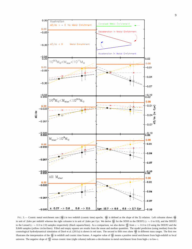
We derive the metallicity evolution in units of “dex per red-shift” and “dex per Gyr” using both the mean and medianvalues. The metallicity evolution can be characterized by theslope (dZdz) of theZz plot. We computedZdz for two redshiftranges:z ∼ 0 → 0.8 (SDSS to DEEP2) andz ∼ 0.8 →∼2.5(DEEP2 to Lensed galaxies). As a comparison, we also de-rive dZ

dz from z ∼ 0.8 to 2.5 using the DEEP2 and the Erb06samples (yellow circles/lines in Figure 3). We derive sepa-rate evolutions for different mass bins. We show our result inFigure 3.

A positive metallicity evolution, i.e., metals enrich galaxiesfrom high-z to the local universe, is robustly found in all massbins fromz ∼ 0.8 → 0. This positive evolution is indicatedby the negative values ofdZdz (or dZ

dz(Gyr) ) in Figure 3. The

negative signs (both mean and median) ofdZdz are significant

at>5 σ of the measurement errors fromz ∼ 0.8 → 0. Fromz ∼ 2.5 to 0.8, however,dZdz is marginally smaller than zero atthe∼1 σ level from the Lensed→ DEEP2 samples. If usingthe Erb06→ DEEP2 samples, the metallicity evolution (dZ

dz )from z ∼ 2.5 to 0.8 is consistent with zero within∼1σ of themeasurement errors. The reason that there is no metallicityevolution from thez ∼ 2 Erb06→ z ∼ 0.8 DEEP2 samplesmay be due to the UV-selected sample of Erb06 being biasedtowards more metal-rich galaxies.

The right column of Figure 3 is used to interpret the de-celeration/acceleration in metal enrichment. Decelerationmeans the metal enrichment rate (dZdz(Gyr)=∆ dex Gyr−1) is

8

TABLE 2MEDIAN /MEAN REDSHIFT AND METALLICITY OF THE SAMPLES

Sample Redshift Metallicity (12 + log(O/H))> 107M⊙(all) > 109M⊙ 109−9.5M⊙ 109.5−11M⊙ 109−10M⊙ 1010−11M⊙

MeanSDSS 0.071±0.016 8.589±0.001 8.616±0.001 8.475±0.002 8.666±0.001 8.589±0.001 8.731±0.001

DEEP2 0.782±0.018 8.459±0.004 8.464±0.004 8.373±0.006 8.512±0.005 8.425±0.004 8.585±0.006Erb06 2.26±0.17 8.418±0.051 8.418±0.050 8.265±0.046 8.495±0.030 8.316±0.052 8.520±0.028Lensed 1.91± 0.63 8.274±0.045 8.309±0.049 8.296±0.090 8.336±0.066 8.313±0.083 8.309±0.086

MedianSDSS 0.072 8.631±0.001 8.646±0.001 8.475±0.003 8.677±0.001 8.617±0.001 8.730±0.001

DEEP2 0.783 8.465±0.005 8.472±0.006 8.362±0.009 8.537±0.008 8.421±0.008 8.614±0.006Erb06 · · · 8.459±0.065 8.459±0.065 8.297±0.056 8.515±0.048 8.319±0.008 8.521±0.043Lensed 2.07 8.286±0.059 8.335±0.063 8.303±0.106 8.346±0.085 8.313±0.083 8.379±0.094

NOTE. — The errors for the redshift are the1σ standard deviation of the sample redshift distribution (not the σ of themean/median). The errors for the metallicity are the1σ standard deviation of the mean/median from bootstrapping.

dropping from high-z to low-z. Using our lensed galax-ies, the mean rise in metallicity is0.055 ± 0.014 dex Gyr−1

for z ∼ 2.5 → 0.8, and 0.022 ± 0.001 dex Gyr−1 forz ∼ 0.8 → 0. The Mann-Whitney test shows that the meanrises in metallicity are larger forz ∼ 2.5 → 0.8 than forz ∼ 0.8 → 0 at a significance level of 95% for the highmass bins (109.5 M⊙ <M⋆ <1011 M⊙). For lower mass bins,the hypothesis that the metal enrichment rates are the samefor z ∼ 2.5 → 0.8 andz ∼ 0.8 → 0 can not be rejectedat the 95% confidence level, i.e, there is no difference in themetal enrichment rates for the lower mass bin. Interestingly,if the Erb06 sample is used instead of the lensed sample, thehypothesis that the metal enrichment rates are the same forz ∼ 2.5 → 0.8 and z ∼ 0.8 → 0 can not be rejectedat the 95% confidence level for all mass bins. This meansthat statistically, the metal enrichment rates are the sameforz ∼ 2.5 → 0.8 andz ∼ 0.8 → 0 for all mass bins from theErb06→ DEEP2→ SDSS samples.

The clear trend of the average/median metallicity in galax-ies rising from high-redshift to the local universe is not sur-prising. Observations based on absorption lines have showna continuing fall in metallicity using the damped Lyα absorp-tion (DLA) galaxies at higher redshifts (z ∼ 2 − 5) (e.g.,Songaila & Cowie 2002; Rafelski et al. 2012). There are sev-eral physical reasons to expect that high-z galaxies are lessmetal-enriched: (1) high-z galaxies are younger, have highergas fractions, and have gone through less generations of starformation than local galaxies; (2) high-z galaxies may bestill accreting a large amount of metal-poor pristine gas fromthe environment, hence have lower average metallicities; (3)high-z galaxies may have more powerful outflows that drivethe metals out of the galaxy. It is likely that all of these mech-anisms have played a role in diluting the metal content at highredshifts.

6.2. Comparison between theZz Relation and Theory

We compare our observations with model predictions fromthe cosmological hydrodynamic simulations of Dave et al.(2011a,b). These models are built within a canonical hier-archical structure formation context. The models take intoaccount the important feedback of outflows by implement-ing an observation-motivated momentum-driven wind model(Oppenheimer & Dave 2008). The effect of inflows and merg-ers are included in the hierarchical structure formation ofthe simulations. Galactic outflows are dealt specifically inthe momentum-driven wind models. Dave & Oppenheimer

(2007) found that the outflows are key to regulating metallic-ity, while inflows play a second-order regulation role.

The model of Dave et al. (2011a) focuses on the metalcontent of star-forming galaxies. Compared with the previ-ous work of Dave & Oppenheimer (2007), the new simula-tions employ the most up-to-date treatment for supernova andAGB star enrichment, and include an improved version of themomentum-driven wind models (thevzw model) where thewind properties are derived based on host galaxy masses (Op-penheimer & Dave 2008). The model metallicity in Daveet al. (2011a) is defined as the SFR-weighted metallicity ofall gas particles in the identified simulated galaxies. Thismodel metallicity can be compared directly with the metal-licity we observe in star-forming galaxies after a constantoff-set normalization to account for the uncertainty in the abso-lute metallicity scale (Kewley & Ellison 2008). The offset isobtained by matching the model metallicity with the SDSSmetallicity. Note that the model has a galaxy mass resolu-tion limit of M⋆ ∼109 M⊙. For theZz plot, we normalizethe model metallicity with the median SDSS metallicity com-puted from all SDSS galaxies>109 M⊙. For the MZ rela-tion in Section 7, we normalize the model metallicity with theSDSS metallicity at the stellar mass of 1010 M⊙.

We compute the median metallicities of the Dave et al.(2011a) model outputs in redshift bins fromz = 0 to z = 3with an increment of 0.1. The median metallicities with 1σspread (defined as including 68% of the data) of the model ateach redshift are overlaid on the observational data in theZzplot.

We compare our observations with the model prediction in3 ways:

(1) We compare the observed median metallicity with themodel median metallicity. We see that for the lower massbins (109−9.5, 109−10 M⊙), the median of the model metal-licity is consistent with the median of the observed metallic-ity within the observational errors. However, for higher massbins, the model over-predicts the metallicity at all redshifts.The over-prediction is most significant in the highest mass binof 1010−11 M⊙, where the Student’s t-statistic shows that themodel distributions have significantly different means than theobservational data at all redshifts, with a probability of being achance difference of< 10−8, < 10−8, 1.7%, 5.7% for SDSS,DEEP2, the Lensed, and the Erb06 samples respectively. Forthe alternative high-mass bin of 109.5−11 M⊙, the model alsoover-predicts the observed metallicity except for the Erb06sample, with a chance difference between the model and ob-

9

x

FIG. 3.— Cosmic metal enrichment rate (dZ

dz ) in two redshift (cosmic time) epochs.dZdz is defined as the slope of theZz relation. Left coloumn showsdZ

dzin unit of ∆dex per redshift whereas the right coloumn is in unit of∆dex per Gyr. We derivedZ

dz for the SDSS to the DEEP2 (z ∼ 0 to 0.8), and the DEEP2

to the Lensed (z ∼ 0.8 to 2.0) samples respectively (black squares/lines). As a comparison, we also derivedZdz from z ∼ 0.8 to 2.0 using the DEEP2 and the

Erb06 samples (yellow circles/lines). Filled and empty squares are results from the mean and median quantities. The model prediction (using median) from thecosmological hydrodynamical simulation of Dave et al. (2011a) is shown in red stars. The second to fifth rows showdZ

dz in different mass ranges. The first row

illustrates the interpretation of thedZdz in redshift and cosmic time frames. A negative value ofdZ

dz means a positive metal enrichment from high-redshift to local

universe. The negative slope ofdZ

dz versus cosmic time (right column) indicates a decelerationin metal enrichment from from high-z to low-z.

10

servations of< 10−8, < 10−8, 1.7%, 8.9%, 93% for SDSS,DEEP2, the Lensed, and the Erb06 samples respectively.

(2) We compare the scatter of the observed metallicity (or-ange error bars onZzplot) with the scatter of the models (reddashed lines). For all the samples, the 1σ scatter of the datafrom the SDSS (z ∼ 0), DEEP2(z ∼ 0.8), and the Lensedsample (z ∼ 2) are: 0.13, 0.15, and 0.15 dex; whereas the1σ model scatter is 0.23, 0.19, and 0.14 dex. We find that theobserved metallicity scatter is increasing systematically as afunction of redshift for the high mass bins whereas the modeldoes not predict such a trend: 0.10, 0.14, 0.17 dex c.f. model0.17, 0.15, 0.12 dex; 109.5−11 M⊙ and 0.07, 0.12, 0.18 dexc.f. model 0.12, 0.11, 0.10 dex ; 1010−11 M⊙ from SDSS→DEEP2→ the Lensed sample. Our observed scatter is in tunewith the work of Nagamine et al. (2001) in which the pre-dicted stellar metallicity scatter increases with redshift. Notethat our lensed samples are still small and have large mea-surement errors in metallicity (∼ 0.2 dex). The discrepancybetween the observed scatter and models needs to be furtherconfirmed with a larger sample.

(3) We compare the observed slope (dZdz) of theZzplot with

the model predictions (Figure 3). We find the observeddZdz is

consistent with the model prediction within the observationalerrors for the undivided sample of all masses>109.0 M⊙.However, when divided into mass bins, the model predictsa slower enrichment than observations fromz ∼ 0 → 0.8 forthe lower mass bin of 109.0−9.5 M⊙, and fromz ∼ 0.8 → 2.5for the higher mass bin of 109.5−11 M⊙ at a 95% significancelevel.

Dave et al. (2011) showed that their models over-predict themetallicities for the highest mass galaxies in the SDSS. Theysuggested that either (1) an additional feedback mechanismmight be needed to suppress star formation in the most mas-sive galaxies; or (2) wind recycling may be bringing in highlyenriched material that elevates the galaxy metallicities.It isunclear from our data which (if any) of these interpretationsis correct. Additional theoretical investigations specificallyfocusing on metallicities in the most massive active galaxiesare needed to determine the true nature of this discrepancy.

7. EVOLUTION OF THE MASS-METALLICITY RELATION

7.1. The Observational Limit of the Mass-MetallicityRelation

For the N2 based metallicity, there is a limiting metallicitybelow which the [NII ] line is too weak to be detected. Since[N II ] is the weakest of the Hα +[N II ] lines, it is thereforethe flux of [N II ] that drives the metallicity detection limit.Thus, for a given instrument sensitivity, there is a region onthe mass-metallicity relation that is observationally unobtain-able. Based on a few simple assumptions, we can derive theboundary of this region as follows.

Observations have shown that there is a positive correlationbetween the stellar massM⋆ andSFR (Noeske et al. 2007b;Elbaz et al. 2011; Wuyts et al. 2011). One explanation fortheM⋆ vs. SFR relation is that more massive galaxies haveearlier onset of initial star formation with shorter timescalesof exponential decay (Noeske et al. 2007a; Zahid et al. 2012).The shape and amplitude of the SFR vs.M⋆ relation at dif-ferent redshiftz can be characterized by two parametersδ(z)andγ(z), whereδ(z) is the logarithm of the SFR at1010M⋆

andγ(z) is the power law index (Zahid et al. 2012).

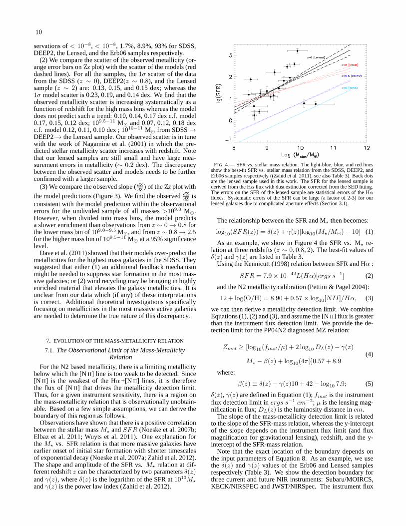
FIG. 4.— SFR vs. stellar mass relation. The light-blue, blue, and red linesshow the best-fit SFR vs. stellar mass relation from the SDSS,DEEP2, andErb06 samples respectively ((Zahid et al. 2011), see also Table 3). Back dotsare the lensed sample used in this work. The SFR for the lensedsample isderived from the Hα flux with dust extinction corrected from the SED fitting.The errors on the SFR of the lensed sample are statistical errors of the Hαfluxes. Systematic errors of the SFR can be large (a factor of 2-3) for ourlensed galaxies due to complicated aperture effects (Section 3.1).

The relationship between the SFR and M⋆ then becomes:

log10(SFR(z)) = δ(z) + γ(z)[log10(M⋆/M⊙)− 10] (1)

As an example, we show in Figure 4 the SFR vs. M⋆ re-lation at three redshifts (z ∼ 0, 0.8, 2). The best-fit values ofδ(z) andγ(z) are listed in Table 3.

Using the Kennicutt (1998) relation between SFR and Hα :

SFR = 7.9× 10−42L(Hα)[ergs s−1] (2)

and the N2 metallicity calibration (Pettini & Pagel 2004):

12 + log(O/H) = 8.90 + 0.57× log10[NII]/Hα, (3)

we can then derive a metallicity detection limit. We combineEquations (1), (2) and (3), and assume the [NII ] flux is greaterthan the instrument flux detection limit. We provide the de-tection limit for the PP04N2 diagnosed MZ relation:

Zmet ≥ [log10(finst/µ) + 2 log10 DL(z)− γ(z)

M⋆ − β(z) + log10(4π)]0.57 + 8.9(4)

where:

β(z) ≡ δ(z)− γ(z)10 + 42− log10 7.9; (5)

δ(z), γ(z) are defined in Equation (1);finst is the instrumentflux detection limit inergs s−1 cm−2; µ is the lensing mag-nification in flux;DL(z) is the luminosity distance incm.

The slope of the mass-metallicity detection limit is relatedto the slope of the SFR-mass relation, whereas the y-interceptof the slope depends on the instrument flux limit (and fluxmagnification for gravitational lensing), redshift, and the y-intercept of the SFR-mass relation.

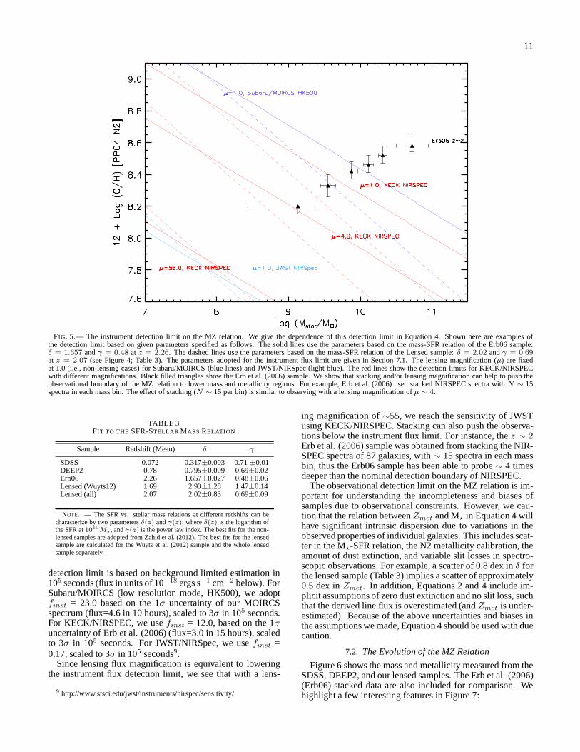
Note that the exact location of the boundary depends onthe input parameters of Equation 8. As an example, we usethe δ(z) andγ(z) values of the Erb06 and Lensed samplesrespectively (Table 3). We show the detection boundary forthree current and future NIR instruments: Subaru/MOIRCS,KECK/NIRSPEC and JWST/NIRSpec. The instrument flux

11

FIG. 5.— The instrument detection limit on the MZ relation. We give the dependence of this detection limit in Equation 4. Shown here are examples ofthe detection limit based on given parameters specified as follows. The solid lines use the parameters based on the mass-SFR relation of the Erb06 sample:δ = 1.657 andγ = 0.48 at z = 2.26. The dashed lines use the parameters based on the mass-SFR relation of the Lensed sample:δ = 2.02 andγ = 0.69at z = 2.07 (see Figure 4; Table 3). The parameters adopted for the instrument flux limit are given in Section 7.1. The lensing magnification (µ) are fixedat 1.0 (i.e., non-lensing cases) for Subaru/MOIRCS (blue lines) and JWST/NIRSpec (light blue). The red lines show the detection limits for KECK/NIRSPECwith different magnifications. Black filled triangles show the Erb et al. (2006) sample. We show that stacking and/or lensing magnification can help to push theobservational boundary of the MZ relation to lower mass and metallicity regions. For example, Erb et al. (2006) used stacked NIRSPEC spectra withN ∼ 15spectra in each mass bin. The effect of stacking (N ∼ 15 per bin) is similar to observing with a lensing magnification ofµ ∼ 4.

TABLE 3FIT TO THE SFR-STELLAR MASS RELATION

Sample Redshift (Mean) δ γ

SDSS 0.072 0.317±0.003 0.71±0.01DEEP2 0.78 0.795±0.009 0.69±0.02Erb06 2.26 1.657±0.027 0.48±0.06Lensed (Wuyts12) 1.69 2.93±1.28 1.47±0.14Lensed (all) 2.07 2.02±0.83 0.69±0.09

NOTE. — The SFR vs. stellar mass relations at different redshiftscan becharacterize by two parametersδ(z) andγ(z), whereδ(z) is the logarithm ofthe SFR at1010M⋆, andγ(z) is the power law index. The best fits for the non-lensed samples are adopted from Zahid et al. (2012). The bestfits for the lensedsample are calculated for the Wuyts et al. (2012) sample and the whole lensedsample separately.

detection limit is based on background limited estimation in105 seconds (flux in units of 10−18 ergs s−1 cm−2 below). ForSubaru/MOIRCS (low resolution mode, HK500), we adoptfinst = 23.0 based on the 1σ uncertainty of our MOIRCSspectrum (flux=4.6 in 10 hours), scaled to 3σ in 105 seconds.For KECK/NIRSPEC, we usefinst = 12.0, based on the 1σuncertainty of Erb et al. (2006) (flux=3.0 in 15 hours), scaledto 3σ in 105 seconds. For JWST/NIRSpec, we usefinst =0.17, scaled to 3σ in 105 seconds9.

Since lensing flux magnification is equivalent to loweringthe instrument flux detection limit, we see that with a lens-

9 http://www.stsci.edu/jwst/instruments/nirspec/sensitivity/

ing magnification of∼55, we reach the sensitivity of JWSTusing KECK/NIRSPEC. Stacking can also push the observa-tions below the instrument flux limit. For instance, thez ∼ 2Erb et al. (2006) sample was obtained from stacking the NIR-SPEC spectra of 87 galaxies, with∼ 15 spectra in each massbin, thus the Erb06 sample has been able to probe∼ 4 timesdeeper than the nominal detection boundary of NIRSPEC.

The observational detection limit on the MZ relation is im-portant for understanding the incompleteness and biases ofsamples due to observational constraints. However, we cau-tion that the relation betweenZmet and M⋆ in Equation 4 willhave significant intrinsic dispersion due to variations in theobserved properties of individual galaxies. This includesscat-ter in the M⋆-SFR relation, the N2 metallicity calibration, theamount of dust extinction, and variable slit losses in spectro-scopic observations. For example, a scatter of 0.8 dex inδ forthe lensed sample (Table 3) implies a scatter of approximately0.5 dex inZmet. In addition, Equations 2 and 4 include im-plicit assumptions of zero dust extinction and no slit loss,suchthat the derived line flux is overestimated (andZmet is under-estimated). Because of the above uncertainties and biases inthe assumptions we made, Equation 4 should be used with duecaution.

7.2. The Evolution of the MZ Relation

Figure 6 shows the mass and metallicity measured from theSDSS, DEEP2, and our lensed samples. The Erb et al. (2006)(Erb06) stacked data are also included for comparison. Wehighlight a few interesting features in Figure 7:

12

(1) To first order, the MZ relation still exists atz ∼ 2,i.e., more massive systems are more metal rich. The Pearsoncorrelation coefficient isr = 0.33349, with a probability ofbeing a chance correlation ofP = 17%. A simple linear fitto the lensed sample yields a slope of 0.164±0.033, with ay-intercept of 6.8±0.3.

(2) All z > 1 samples show evidence of evolution to lowermetallicities at fixed stellar masses. At high stellar mass(M⋆ >1010 M⊙), the lensed sample has a mean metallicityand a standard deviation of the mean of 8.41±0.05, whereasthe mean and standard deviation of the mean for the Erb06sample is 8.52±0.03. The lensed sample is offset to lowermetallicity by 0.11±0.06 dex compared to the Erb06 sample.This slight offset may indicate the selection differencebetween the UV-selected (potentially more dusty and metalrich) sample and the lensed sample (less biased towards UVbright systems).

(3) At lower mass (M⋆ <109.4 M⊙), our lensed sampleprovides 12 individual metallicity measurements atz > 1.The mean metallicity of the galaxies with M⋆ <109.4 M⊙ is8.25±0.05, roughly consistent with the<8.20 upper limit ofthe stacked metallicity of the lowest mass bin (M⋆ ∼109.1

M⊙) of the Erb06 galaxies.

(4) Compared with the Erb06 galaxies, there is a lack ofthe highest mass galaxies in our lensed sample. We notethat there is only 1 object with M⋆ >1010.4 M⊙ amongall three lensed samples combined. The lensed sampleis less affected by the color selection and may be morerepresentative of the mass distribution of high-z galaxies. Inthe hierarchical galaxy formation paradigm, galaxies growtheir masses with time. The number density of massivegalaxies at high redshift is smaller than atz ∼ 0, thusthe number of massive lensed galaxies is small. Selectioncriteria such as the UV-color selection of the Erb06 andSINs (Genzel et al. 2011) galaxies can be applied to tar-get the high-mass galaxies on the MZ relation at high redshift.

7.3. Comparison with Theoretical MZ Relations

Understanding the origins of the MZ relation has been thedriver of copious theoretical work. Based on the idea thatmetallicities are mainly driven by an equilibrium among stel-lar enrichment, infall and outflow, Finlator & Dave (2008) de-veloped smoothed particle hydrodynamic simulations. Theyfound that the inclusion of a momentum-driven wind model(vzw) fits best to thez ∼ 2 MZ relations compared toother outflow/wind models. The updated version of theirvzwmodel is described in detail in Dave et al. (2011a). We over-lay the Dave et al. (2011a)vzw model outputs on the MZrelation in Figure 7. We find that the model does not repro-duce the MZ redshift evolution seen in our observations. Weprovide possible explanations as follows.

Kewley & Ellison (2008) found that both the shape andscatter of the MZ relation vary significantly among differ-ent metallicity diagnostics. This poses a tricky normaliza-tion problem when comparing models to observations. Forexample, a model output may fit the MZ relation slope fromone strong-line diagnostic, but fail to fit the MZ relation fromanother diagnostic, which may have a very different slope.This is exactly what we are seeing on the left panel of Fig-

ure 7. Dave et al. (2011a) applied a constant offset of themodel metallicities by matching the amplitude of the modelMZ relation atz ∼ 0 with the observed local MZ relation ofTremonti et al. (2004, T04) at the stellar mass of 1010 M⊙.Dave et al. (2011a) found that the characteristic shape andscatter of the MZ relation from thevzw model matches theT04 MZ relation between 109.0 M⊙ <M⋆ <1011.0 withinthe 1σ model and observational scatter. However, since boththe slope and amplitude of the T04 SDSS MZ relation aresignificantly larger than the SDSS MZ relation derived usingthe PP04N2 method (Kewley & Ellison 2008), the PP04N2-normalized MZ relation from the model does not recover thelocal MZ relation within1σ.

In addition, the stellar mass measurements from differentmethods may cause a systematic offsets in the x-direction ofthe MZ relation (Zahid et al. 2011). As a result, even thoughthe shape, scatter, and evolution with redshifts are indepen-dent predictions from the model, systematic uncertaintiesinmetallicity diagnostics and stellar mass estimates do not al-low the shape to be constrained separately.

In the right panel of Figure 7, we allow the model slope (α),metallicity amplitude (Z), and stellar mass (M∗) to changeslightly so that it fits the local SDSS MZ relation. As-suming that this change in slope (∆α), and x, y amplitudes(∆Z,∆M∗) are caused by the systematic offsets in observa-tions, then the same∆α, ∆Z, and∆M∗ can be applied tomodel MZ relations at other redshifts. Although normalizingthe model MZ relation in this way will make the model loseprediction power for the shape of the MZ relation, it at leastleaves the redshift evolution of the MZ relation as a testablemodel output.

Despite the normalization correction, we see from Figure 7that the models predict less evolution from z∼ 2 to z∼ 0 thanthe observed MZ relation. To quantify, we divide the modeldata into two mass bins and derive the mean and 1σ scatter ineach mass bin as a function of redshift. We define the “meanevolved metallicity” on the MZ relation as the difference be-tween the mean metallicity at redshiftz and the mean metal-licity at z ∼ 0 at a fixed stellar mass (log (O/H) [z∼0] −log (O/H) [z∼2]). The “mean evolved metallicity” errors arecalculated based on the standard errors of the mean.

In Figure 8 we plot the “mean evolved metallicity”as a function of redshift for two mass bins: 109.0

M⊙ <M⋆ <109.5 M⊙, 109.5 M⊙ <M⋆ <1011 M⊙. We cal-culate the observed “mean evolved metallicity” for DEEP2and our lensed sample in the same mass bins. We see thatthe observed mean evolution of the lensed sample are largelyuncertain and no conclusion between the model and obser-vational data can be drawn. However, the DEEP2 data arewell-constrained and can be compared with the model.

We find that atz ∼ 0.8, the mean evolved metallicity ofthe high-mass galaxies are consistent with the mean evolvedmetallicity of the models. The observed mean evolved metal-licity of the low-mass bin galaxies is∼ 0.12 dex larger thanthe mean evolved metallicity of the models in the same massbins.

8. COMPARE WITH PREVIOUS WORK IN LITERATURE

In this Section, we compare our findings with previouswork on the evolution of the MZ relation.

For low masses (109 M⊙), we find a larger enrichment (i.e.,smaller decrease in metallicity) betweenz ∼ 2 → 0 thaneither the non-lensed sample of Maiolino et al. (2008) (0.15dex c.f. 0.6 dex) or the lensed sample of Wuyts et al. (2012);

13

FIG. 6.— Left: the observed MZ relation. Black symbols are the lensed galaxy sample atz > 1. Specifically, the squares are from this work; the stars are fromWuyts et al. (2012), and the diamonds are from Richard et al. (2011). The orange triangles show the Erb et al. (2006) sample. The local SDSS relation and its1-sigma range are drawn in purple lines. Thez ∼ 0.8 DEEP2 relations from Zahid et al. (2011) are drawn in purple dots. Right: the best fit to the MZ relation.A second degree polynomial function is fit to the SDSSS, DEEEP2, and Erb06 samples. A simple linear function is fit to the lensed sample. Thez > 1 lenseddata are binned in 5 mass bins (symbol: red star) and the median and 1σ standard deviation of each bin are plotted on top of the linear fit.

FIG. 7.— Model predictions of the MZ relation. The data symbols are the same as those used in Figure 6. The small green and lightblue dots are thecosmological hydrodynamic simulations with momentum-conserving wind models from Dave et al. (2011a). The difference between the left and right panelsare the different normalization methods used. The left panel normalizes the model metallicity to the observed SDSS values by applying a constant offset atMstar ∼ 1010M⊙, whereas the right panel normalizes the model metallicity to the observed SDSS metallicity by allowing a constant shiftin the slope,amplitude and stellar mass. Note that the model has a mass cutoff at 1.1× 109M⊙.

Richard et al. (2011) (0.4 dex). These discrepancies may re-flect differences in metallicity calibrations applied. It is clearthat a larger sample is required to characterize the true meanand spread in metallicities at intermediate redshift. Notethatthe lensed samples are still small and have large measurementerrors in both stellar masses (0.1 to 0.5 dex) and metallicity(∼ 0.2 dex).

For high masses (1010 M⊙), we find similar enrichment (0.4dex) betweenz ∼ 2 → 0 compare to the non-lensed sampleof Maiolino et al. (2008) and the lensed sample of Wuyts et al.(2012); Richard et al. (2011).

We find in Section 6.1 that the deceleration in metalenrichment is significant in the highest mass bin (109.5

M⊙ <M⋆ <1011 M⊙) of our samples. The deceleration inmetal enrichment fromz ∼ 2 → 0.8 to z ∼ 0.8 → 0 isconsistent with the picture that the star formation and massassembly peak between redshift 1 and 3 (Hopkins & Beacom2006). The deceleration is larger by 0.019±0.013 dex Gyr−2

in the high mass bin, suggesting a possible mass-dependencein chemical enrichment, similar to the “downsizing” mass-dependent growth of stellar mass (Cowie et al. 1996; Bundyet al. 2006). In the downsizing picture, more massive galaxiesformed their stars earlier and on shorter timescales comparedwith less massive galaxies (Noeske et al. 2007a). Our obser-vation of the chemical downsizing is consistent with previousmetallicity evolution work (Panter et al. 2008; Maiolino etal.

14

FIG. 8.— The “mean evolved metallicity” as a function of redshift for twomass bins (indicated by four colors). Dashed lines show the median and 1σscatter of the model prediction from Dave et al. (2011a). The observed datafrom DEEP2 and our lensed sample are plotted as filled circles.

2008; Richard et al. 2011; Wuyts et al. 2012).We find that for higher mass bins, the model of Dave et al.

(2011a) over-predicts the metallicity at all redshifts. Theover-prediction is most significant in the highest mass bin of1010−11 M⊙. This conclusion similar to the findings in Daveet al. (2011a,b). In addition, we point out that when compar-ing the model metallicity with the observed metallicity, thereis a normalization problem stemming from the discrepancyamong different metallicity calibrations (Section 7.3).

We note the evolution of the MZ relation is based on an en-semble of the averaged SFR weighted metallicity of the star-forming galaxies at each epoch. The MZ relation does notreflect an evolutionary track of individual galaxies. We areprobably seeing a different population of galaxies at each red-shift (Brooks et al. 2007; Conroy et al. 2008). For example, a∼1010.5 M⊙ massive galaxy atz ∼2 will most likely evolveinto an elliptical galaxy in the local universe and will not ap-pear on the local MZ relation. On the other hand, to trace theprogenitor of a∼1011 M⊙ massive galaxy today, we need toobserve a∼109.5 M⊙ galaxy atz ∼2 (Zahid et al. 2012).

It is clear that gravitational lensing has the power to probelower stellar masses than current color selection techniques.Larger lensed samples with high-quality observations are re-quired to reduce the measurement errors.

9. SUMMARY

To study the evolution of the overall metallicity and MZ re-lation as a function of redshift, it is critical to remove thesys-tematics among different redshift samples. The major caveatsin current MZ relation studies atz >1 are: (1) metallicityis not based on the same diagnostic method; (2) stellar massis not derived using the same method; (3) the samples are se-lected differently and selection effects on mass and metallicityare poorly understood. In this paper, we attempt to minimizethese issues by re-calculating the stellar mass and metallic-ity consistently, and by expanding the lens-selected sample atz >1. We aim to present a reliable observational picture of themetallicity evolution of star forming galaxies as a function ofstellar mass between0 < z < 3. We find that:

• There is a clear evolution in the mean and medianmetallicities of star-forming galaxies as a function of

redshift. The mean metallicity falls by∼ 0.18 dex fromredshift 0 to 1 and falls further by∼ 0.16 dex from red-shift 1 to 2.

• A more rapid evolution is seen betweenz ∼ 1 → 3than z ∼ 0 → 1 for the high-mass galaxies (109.5

M⊙ <M⋆ <1011 M⊙), with almost twice as much en-richment betweenz ∼ 1 → 3 than betweenz ∼ 1 → 0.

• The deceleration in metal enrichment fromz ∼ 2 →0.8 to z ∼ 0.8 → 0 is significant in the high-massgalaxies (109.5 M⊙ <M⋆ <1011 M⊙), consistent witha mass-dependent chemical enrichment.

• We compare the metallicity evolution of star-forminggalaxies fromz = 0 → 3 with the most recentcosmological hydrodynamic simulations. We see thatthe model metallicity is consistent with the observedmetallicity within the observational error for the lowmass bins. However, for higher mass bins, the modelover-predicts the metallicity at all redshifts. The over-prediction is most significant in the highest mass bin of1010−11 M⊙. Further theoretical investigation into themetallicity of the highest mass galaxies is required todetermine the cause of this discrepancy.

• The median metallicity of the lensed sample is0.35±0.06 dex lower than local SDSS galaxies and0.28±0.06 dex lower than thez ∼ 0.8 DEEP2 galaxies.

• Cosmological hydrodynamic simulation (Dave et al.2011a) does not agree with the evolutions of the ob-served MZ relation based on the PP04N2 diagnostic.Whether the model fits the slope of the MZ relation de-pends on the normalization methods used.

This study is based on 6 clear nights of observations on a8-meter telescope, highlighting the efficiency in using lens-selected targets. However, the lensed sample atz > 1 is stillsmall. We aim to significantly increase the sample size overthe years.

We would like to thank the referee for an excellent reportthat has significantly improved this paper. T.-Y. wants tothank the MOIRCS supporting astronomer Ichi Tanaka andKentaro Aoki for their enormous support on the MOIRCSobservations. We thank Youichi Ohyama for scripting theoriginal MOIRCS data reduction pipeline. We are grate-ful to Dave Rommel for providing and explaining to us hismost recent models. T.-Y. wants to thank Jabran Zahid forthe SDSS and DEEP2 data and many insightful discussions.T.-Y. acknowledges a Soroptimist Founder Region Fellow-ship for Women. L.K. acknowledges a NSF Early CAREERAward AST 0748559 and an ARC Future Fellowship awardFT110101052. JR is supported by the Marie Curie Career In-tegration Grant 294074. We wish to recognize and acknowl-edge the very significant cultural role and reverence that thesummit of Mauna Kea has always had within the indigenousHawaiian community.

Facilities: Subaru (MOIRCS)

15

APPENDIX

SLIT LAYOUT, SPECTRA FOR THE LENSED SAMPLE

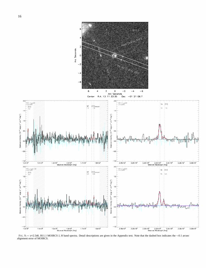
This section presents the slit layouts, reduced and fitted spectra for the newly observed lensed objects in this work. Thelinefitting procedure is described in Section 3.2. For each target, the top panel shows the HST ACS 475W broad-band image of thelensed target. The slit layouts with different positional angles are drawn in white boxes. The bottom panel(s) show(s) the finalreduced 1D spectrum(a) zoomed in for emission line vicinities. The black line is the observed spectrum for the target. The cyanline is the noise spectrum extracted from object-free pixels of the final 2D spectrum. Tilted grey mesh lines indicate spectralranges where the sky absorption is severe. Emission lines falling in these spectral windows suffer from large uncertainties intelluric absorption correction. The blue horizontal line is the continuum fit using first order polynomial function after blankingout the severe sky absorption region. The red lines overplotted on the emission lines are the overall Gaussian fit, with the bluelines show individual components of the multiple Gaussian functions. Vertical dashed lines show the center of the Gaussianprofile for each emission line. The S/N of each line are markedunder the emission line labels. Note that for lines with S/N<3,the fit is rejected and a 3-σ upper limit is derived.

Brief remarks on individual objects (see also Table 2 and 3 for more information):

• Figure 9 and 10, B11 (888351) : this is a resolved galaxy with spiral-like structure at z = 2.540 ± 0.006. As reportedin Broadhurst et al. (2005), It is likely to be the most distant known spiral galaxy so far. B11 has 3 multiple images. Wehave observed B11.1, and B11.2, with two slit orientations on each image respectively. Different slit orientation yieldsvery different line ratios, implying possible gradients. Our IFU follow-up observations are in progress to reveal the detailsof this 2.6-Gyr-old spiral.

• Figure 11 and 12, B2 (860331): this is one of the interesting systems reported in Fryeet al. (2007). It has 5 multipleimages, and is only 2′′ away from another five-image lensed system, “The Sextet Arcs” at z=3.038. We have observedB2.1 and B2.2 and detected strong Hα and [OIII ] lines in both of them, yielding a redshift of2.537 ± 0.006, consistentwith the redshiftz = 2.534 measured from the absorption lines ([CII ] λ1334, [SiII ] λ1527) in Frye et al. (2007).

• Figure 13, MS1 (869328): We have detected a 7-σ [O III ] line and determined its redshift to bez = 2.534± 0.010.

• Figure 14, B29 (884331): this is a lensed system with 5 multiple images. We observed B29.3, the brightest of the fiveimages. The overall surface brightness of the B29.3 arc is very low, We have observed a 10-σ Hα and an upper limit for[N II ], placing it atz = 2.633± 0.010.

• Figure 15, G3: this lensed arc with a bright knot has no recorded redshift before this study. It was put on one of the extraslits during mask designing. We have detected a 8-σ [O III ] line and determined its redshift to bez = 2.540± 0.010.

• Figure 16, Ms-Jm7 (865359): We detected [OII ] Hβ [O III ] Hα and an upper limit for [NII ] placing it at redshiftz = 2.588± 0.006.

• Figure 17 and 18, B5 (892339, 870346): it has three multiple images, of which we observed B5.1and B5.3. Two slitorientations were observed for B5.1, the final spectrum for B5.1 has combined the two slit orientations weighted by theS/N of HαStrong Hα and upper limit of [NII ] were obtained in both images, yielding a redshift ofz = 2.636± 0.004.

• Figure 19, G2 (894332): two slit orientations were available for G2, with detections of Hβ, [O III ], Hα, and upper limitsfor [O II ] and [N II ]. The redshift measured isz = 1.643± 0.010.

• Figure 20, B12: this blue giant arc has 5 multiple images, andwe observed B12.2. It shows a series of strong emissionlines, with an average redshift ofz = 1.834± 0.006.

• Figure 21, Lensz1.36 (891321): it has a very strong Hα and [NII ] is at noise level, from Hα we derivez = 1.363±0.010.

• Figure 22, MSnewz3: this is a new target observed in Abell 1689, we detect [OII ], Hβ, and [OIII ] at a significant level,yieldingz = 3.007± 0.003.

• Figure 23, B8: this arc has five multiple images in total, and we observed B8.2, detection of [OII ], [O III ], Hα, with Hβand [NII ] as upper limit yields an average redshift ofz = 2.662± 0.006.

• B22.3: a three-image lensed system atz = 1.703± 0.004, this is the first object reported from our LEGMS program, seeYuan & Kewley (2009).

• Figure 24, A68-C27: this is the only object chosen from our unfinished observations on Abell 68. This target has manystrong emission lines.z = 1.762± 0.006. The morphology of C27 shows signs of merger. IFU observation on this targetis in process.

16

FIG. 9.— z=2.540, B11.1 MOIRCS J, H band spectra. Detail descriptions are given in the Appendix text. Note that the dashed boxindicates the∼0.1 arcsecalignment error of MOIRCS.

17

FIG. 10.— z=2.540, B11.2 MOIRCS J, H band spectra. Detail descriptions are given in the Appendix text.

18

FIG. 11.— z=2.537, B2.1, MOIRCS J, H band spectra. Detail descriptions are given in the Appendix text.

19

FIG. 12.— z=2.537, B2.2, MOIRCS J, H band spectra. Detail descriptions are given in the Appendix text.

20

FIG. 13.— z=2.54, MS1, MOIRCS J, H band spectra. Detail descriptions are given in the Appendix text.

FIG. 14.— z=2.633, B29.3, MOIRCS J, H band spectra. Detail descriptions are given in the Appendix text.

21

FIG. 15.— z=2.540, G3, MOIRCS J, H band spectra. Detail descriptions are given in the Appendix text.

FIG. 16.— z=2.588, Jm7, MOIRCS J, H band spectra. Detail descriptions are given in the Appendix text.

22

FIG. 17.— z=2.641, B5.1, MOIRCS J, H band spectra. Note that the reason that the flux of B5.1 in slit position PAn60 is less than PA45 (B5.1+B5.2) is thatthe dithering length of PAn60 was smaller than the separation of 5.1 and 5.2, thus part of the flux of PA45 (B5.1+B5.2) was cancelled out during the ditheringprocess. Detail descriptions are given in the Appendix text.

23

FIG. 18.— z=2.636, B5.3, MOIRCS J, H band spectra. Detail descriptions are given in the Appendix text.

24

FIG. 19.— z=2.643, G2, MOIRCS J, H band spectra. Detail descriptions are given in the Appendix text.

25

FIG. 20.— z=1.834±0.002, B12.2, MOIRCS J, H band spectra. Detail descriptionsare given in the Appendix text.

FIG. 21.— z=1.363, Low-z, MOIRCS J, H band spectra. Detail descriptions are given in the Appendix text.

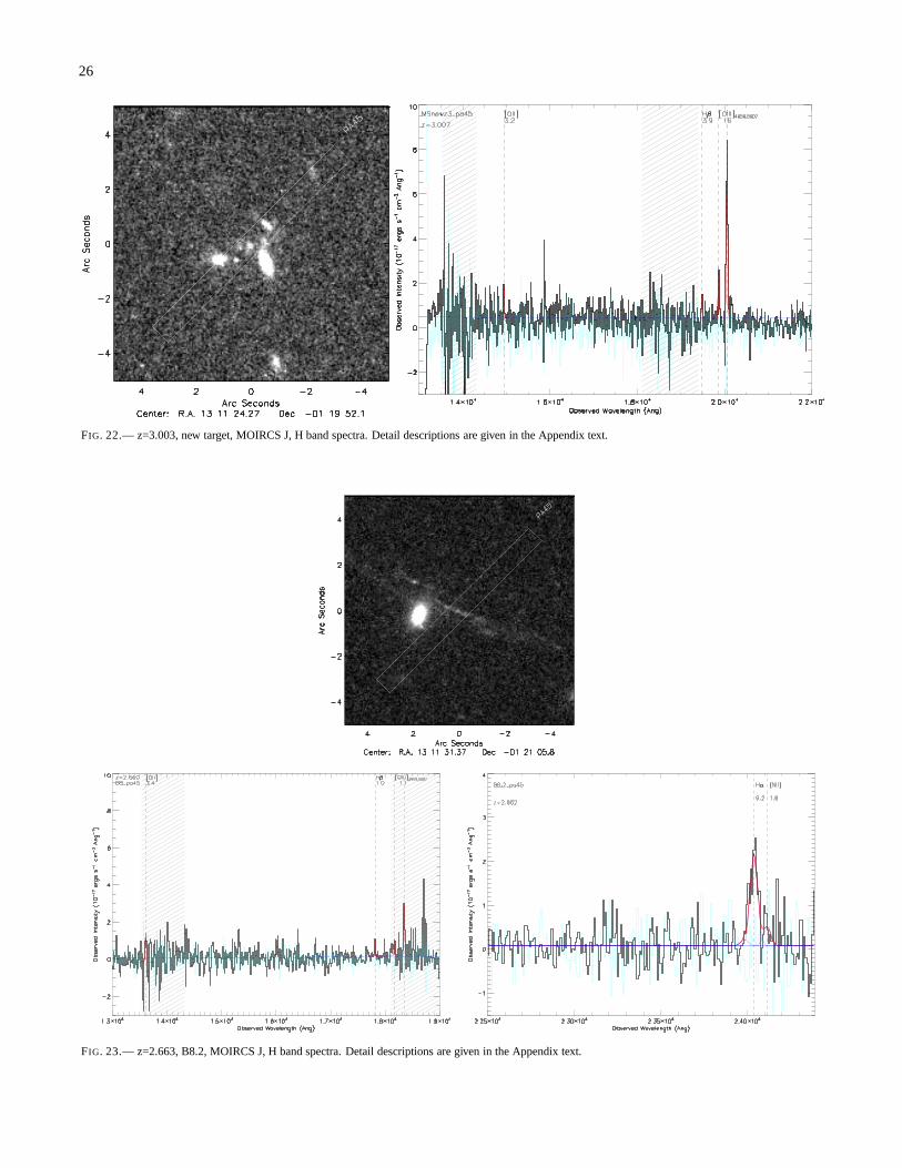
26

FIG. 22.— z=3.003, new target, MOIRCS J, H band spectra. Detail descriptions are given in the Appendix text.

FIG. 23.— z=2.663, B8.2, MOIRCS J, H band spectra. Detail descriptions are given in the Appendix text.

27

FIG. 24.— z=1.763, A68C27, MOIRCS J, H band spectra. Detail descriptions are given in the Appendix text.

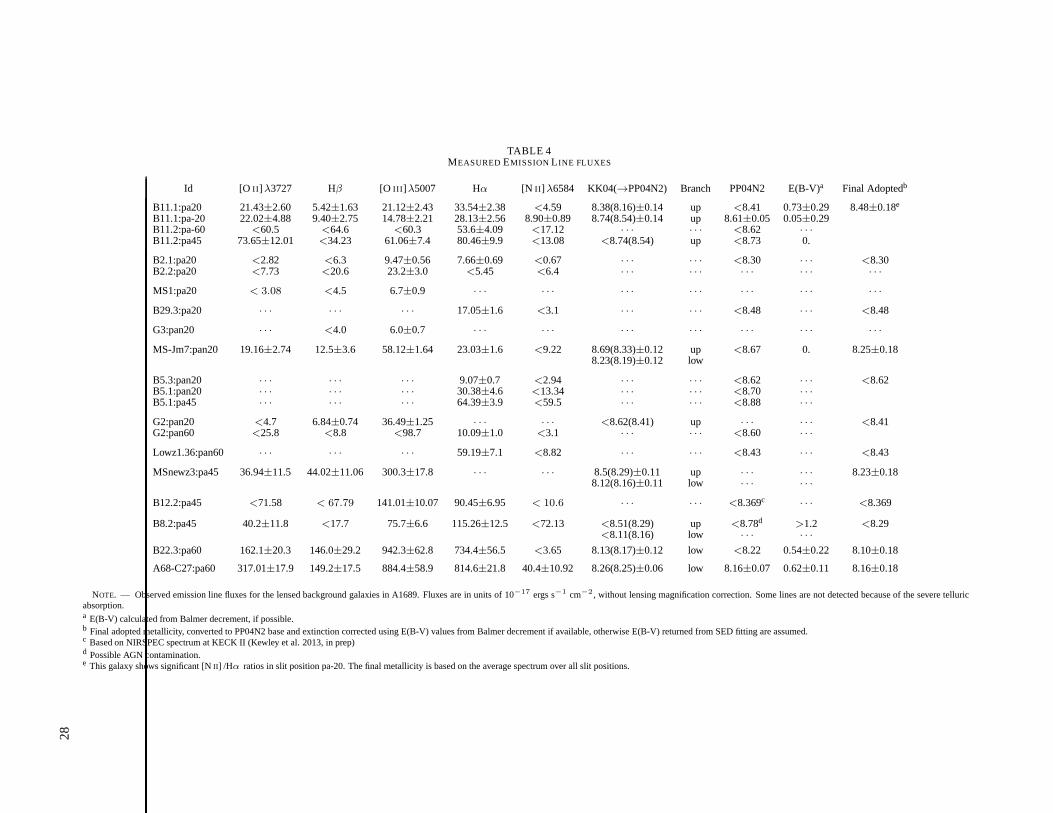
28

TABLE 4MEASUREDEMISSIONL INE FLUXES

Id [O II ] λ3727 Hβ [O III ] λ5007 Hα [N II ] λ6584 KK04(→PP04N2) Branch PP04N2 E(B-V)a Final Adoptedb

B11.1:pa20 21.43±2.60 5.42±1.63 21.12±2.43 33.54±2.38 <4.59 8.38(8.16)±0.14 up <8.41 0.73±0.29 8.48±0.18e

B11.1:pa-20 22.02±4.88 9.40±2.75 14.78±2.21 28.13±2.56 8.90±0.89 8.74(8.54)±0.14 up 8.61±0.05 0.05±0.29B11.2:pa-60 <60.5 <64.6 <60.3 53.6±4.09 <17.12 · · · · · · <8.62 · · ·

B11.2:pa45 73.65±12.01 <34.23 61.06±7.4 80.46±9.9 <13.08 <8.74(8.54) up <8.73 0.

B2.1:pa20 <2.82 <6.3 9.47±0.56 7.66±0.69 <0.67 · · · · · · <8.30 · · · <8.30B2.2:pa20 <7.73 <20.6 23.2±3.0 <5.45 <6.4 · · · · · · · · · · · · · · ·

MS1:pa20 < 3.08 <4.5 6.7±0.9 · · · · · · · · · · · · · · · · · · · · ·

B29.3:pa20 · · · · · · · · · 17.05±1.6 <3.1 · · · · · · <8.48 · · · <8.48

G3:pan20 · · · <4.0 6.0±0.7 · · · · · · · · · · · · · · · · · · · · ·

MS-Jm7:pan20 19.16±2.74 12.5±3.6 58.12±1.64 23.03±1.6 <9.22 8.69(8.33)±0.12 up <8.67 0. 8.25±0.188.23(8.19)±0.12 low

B5.3:pan20 · · · · · · · · · 9.07±0.7 <2.94 · · · · · · <8.62 · · · <8.62B5.1:pan20 · · · · · · · · · 30.38±4.6 <13.34 · · · · · · <8.70 · · ·

B5.1:pa45 · · · · · · · · · 64.39±3.9 <59.5 · · · · · · <8.88 · · ·

G2:pan20 <4.7 6.84±0.74 36.49±1.25 · · · · · · <8.62(8.41) up · · · · · · <8.41G2:pan60 <25.8 <8.8 <98.7 10.09±1.0 <3.1 · · · · · · <8.60 · · ·

Lowz1.36:pan60 · · · · · · · · · 59.19±7.1 <8.82 · · · · · · <8.43 · · · <8.43

MSnewz3:pa45 36.94±11.5 44.02±11.06 300.3±17.8 · · · · · · 8.5(8.29)±0.11 up · · · · · · 8.23±0.188.12(8.16)±0.11 low · · · · · ·

B12.2:pa45 <71.58 < 67.79 141.01±10.07 90.45±6.95 < 10.6 · · · · · · <8.369c · · · <8.369

B8.2:pa45 40.2±11.8 <17.7 75.7±6.6 115.26±12.5 <72.13 <8.51(8.29) up <8.78d >1.2 <8.29<8.11(8.16) low · · · · · ·

B22.3:pa60 162.1±20.3 146.0±29.2 942.3±62.8 734.4±56.5 <3.65 8.13(8.17)±0.12 low <8.22 0.54±0.22 8.10±0.18

A68-C27:pa60 317.01±17.9 149.2±17.5 884.4±58.9 814.6±21.8 40.4±10.92 8.26(8.25)±0.06 low 8.16±0.07 0.62±0.11 8.16±0.18

NOTE. — Observed emission line fluxes for the lensed background galaxies in A1689. Fluxes are in units of 10−17 ergs s−1 cm−2, without lensing magnification correction. Some lines are not detected because of the severe telluricabsorption.a E(B-V) calculated from Balmer decrement, if possible.b Final adopted metallicity, converted to PP04N2 base and extinction corrected using E(B-V) values from Balmer decrement if available, otherwise E(B-V) returned from SED fitting are assumed.c Based on NIRSPEC spectrum at KECK II (Kewley et al. 2013, in prep)d Possible AGN contamination.e This galaxy shows significant [NII ] /Hα ratios in slit position pa-20. The final metallicity is basedon the average spectrum over all slit positions.

29

TABLE 5PHYSICAL PROPERTIES OF THELENSEDSAMPLE

ID1 ID2a RA, DEC (J2000) Redshift lg(SFR)b Lensing Magnification log(M∗/M⊙)(M⊙ yr−1) (flux)

B11.1:pa20 888351 13:11:33.336, -01:21:06.94 2.540±0.006 1.08±0.1 11.8±2.7 9.1+0.2−0.3

B11.2:pa45 · · · 13:11:29.053, -01:20:01.26 2.540±0.006 1.42±0.11 13.1±1.8

B2.1:pa20 860331 13:11:26.521, -01:19:55.24 2.537±0.006 0.20±0.03 20.6±1.8 8.2+0.3−0.3

B2.2:pa20 · · · 13:11:32.961, -01:20:25.31 2.537±0.006 · · · 15.0±2.0

MS1:pa20 869328 13:11:28.684,-01:19:42.62 2.534±0.01 · · · 58.3±2.8 8.5+0.1−0.1

B29.3:pa20 884331 13:11:32.164,-01:19:52.53 2.633±0.01 0.43±0.06 22.5±6.9 9.0+0.4−0.5

f

G3:pan20 · · · 13:11:26.219,-01:21:09.64 2.540±0.01 · · · 7.7±0.1 · · ·

MS-Jm7:pan20 865359 13:11:27.600,-01:21:35.00 2.588±0.006 · · · 18.5±3.2 8.0+0.5−0.4

f

B5.3:pan20 892339 13:11:34.109,-01:20:20.90 2.636±0.004 0.47±0.05 14.2±1.3 9.1+0.4−0.2

B5.1:pan60 870346 13:11:29.064,-01:20:48.33 2.641±0.004 1.0±0.05 14.3±0.3

G2 894332 13:11:34.730,-01:19:55.53 1.643±0.01 0.45±0.09 16.7±3.1 8.0+0.3−0.4

Lowz1.36 891321 13:11:33.957,-01:19:15.90 1.363±0.01 0.67±0.11 11.6±2.7 8.9+0.3−0.3

MSnewz3:pa45 · · · 13:11:24.276,-01:19:52.08 3.007±0.003 0.65±0.55 2.9±1.7 8.6+0.3−0.4

f

B12.2:pa45 863348 13:11:27.212,-01:20:51.89 1.834±0.006 1.00±0.05c 56.0±4.4 7.4+0.2−0.0

B8.2:pa45 · · · 13:11:27.212,-01:20:51.89 2.662±0.006 1.36±0.07d 23.7±3.0 8.2+0.5−0.6

f

B22.3:pa60e · · · 13:11:32.4150,-01:21:15.917 1.703±0.006 1.88±0.04 15.5±0.3 8.5+0.2−0.2

A68-C27:pa60 · · · 00:37:04.866,+09:10:29.26 1.762±0.006 2.46±0.1 4.9±1.1 9.6+0.1−0.1

NOTE. — The redshift errors in Table 5 is determined from RMS of different emission line centroids. If the RMS is smaller than 0.006 (for most targets)or if there is only one line fitted, we adopt the systematic error of 0.006 as a conservative estimation for absolute redshift measurements.a ID used in Richard et al. (2012, in prep). The name tags of the objects are chosen to be consistent with the Broadhurst et al.(2005) conventions ifoverlapping.b Corrected for lensing magnification, but without dust extinction correction. We note that the systematic errors of SFR in this work are extremely uncertaindue to complicated aperture correction and flux calibrationin the multi-slit of MOIRCS.c Based on NIRSPEC observationd Possible AGN contamination.e See also Yuan & Kewley (2009)f The IRAC photometry for these sources are not included in thestellar mass calculation due to the difficulty in resolving the lensed image from theadjacent foreground galaxies.

30

REFERENCES

Abazajian, K. N., et al. 2009, ApJS, 182, 543Asplund, M., Grevesse, N., Sauval, A. J., & Scott, P. 2009, ARA&A, 47, 481Baldwin, J. A., Phillips, M. M., & Terlevich, R. 1981, PASP, 93, 5Bertin, E., & Arnouts, S. 1996, A&AS, 117, 393Bertone, S., De Lucia, G., & Thomas, P. A. 2007, MNRAS, 379, 1143Brinchmann, J., Pettini, M., & Charlot, S. 2008, MNRAS, 385,769Broadhurst, T., et al. 2005, ApJ, 621, 53Brooks, A. M., Governato, F., Booth, C. M., Willman, B., Gardner, J. P.,

Wadsley, J., Stinson, G., & Quinn, T. 2007, ApJ, 655, L17Bruzual, G., & Charlot, S. 2003, MNRAS, 344, 1000Bundy, K., et al. 2006, ApJ, 651, 120Calzetti, D., Armus, L., Bohlin, R. C., Kinney, A. L., Koornneef, J., &

Storchi-Bergmann, T. 2000, ApJ, 533, 682Capak, P., et al. 2004, AJ, 127, 180Chabrier, G. 2003, PASP, 115, 763Chapman, S. C., Blain, A. W., Smail, I., & Ivison, R. J. 2005, ApJ, 622, 772Christensen, L., et al. 2012, ArXiv e-printsConroy, C., Shapley, A. E., Tinker, J. L., Santos, M. R., & Lemson, G. 2008,

ApJ, 679, 1192Conselice, C. J., et al. 2007, MNRAS, 381, 962Cowie, L. L., & Barger, A. J. 2008, ApJ, 686, 72Cowie, L. L., Songaila, A., Hu, E. M., & Cohen, J. G. 1996, AJ, 112, 839Daddi, E., Cimatti, A., Renzini, A., Fontana, A., Mignoli, M., Pozzetti, L.,

Tozzi, P., & Zamorani, G. 2004, ApJ, 617, 746Dalcanton, J. J. 2007, ApJ, 658, 941Dave, R., Finlator, K., & Oppenheimer, B. D. 2011a, MNRAS, 416, 1354Dave, R., & Oppenheimer, B. D. 2007, MNRAS, 374, 427Dave, R., Oppenheimer, B. D., & Finlator, K. 2011b, MNRAS, 415, 11Davies, R. I. 2007, MNRAS, 375, 1099Davis, M., et al. 2003, in Society of Photo-Optical Instrumentation

Engineers (SPIE) Conference Series, Vol. 4834, Society of Photo-OpticalInstrumentation Engineers (SPIE) Conference Series, ed. P. Guhathakurta,161–172

De Lucia, G., Kauffmann, G., & White, S. D. M. 2004, MNRAS, 349, 1101Dickinson, M., Papovich, C., Ferguson, H. C., & Budavari, T. 2003, ApJ,

587, 25Edmunds, M. G. 1990, MNRAS, 246, 678Edmunds, M. G., & Greenhow, R. M. 1995, MNRAS, 272, 241Elbaz, D., et al. 2011, A&A, 533, A119Erb, D. K., Pettini, M., Shapley, A. E., Steidel, C. C., Law, D. R., & Reddy,

N. A. 2010, ApJ, 719, 1168Erb, D. K., Shapley, A. E., Pettini, M., Steidel, C. C., Reddy, N. A., &

Adelberger, K. L. 2006, ApJ, 644, 813Erb, D. K., Shapley, A. E., Steidel, C. C., Pettini, M., Adelberger, K. L.,

Hunt, M. P., Moorwood, A. F. M., & Cuby, J.-G. 2003, ApJ, 591, 101Fan, X., et al. 2001, AJ, 121, 54Finlator, K., & Dave, R. 2008, MNRAS, 385, 2181Forster Schreiber, N. M., et al. 2006, ApJ, 645, 1062Forster Schreiber, N. M., Shapley, A. E., Erb, D. K., Genzel, R., Steidel,

C. C., Bouche, N., Cresci, G., & Davies, R. 2011, ApJ, 731, 65Frye, B. L., et al. 2007, ApJ, 665, 921Garnett, D. R. 2002, ApJ, 581, 1019Genzel, R., et al. 2008, ApJ, 687, 59—. 2011, ApJ, 733, 101Grazian, A., et al. 2007, A&A, 465, 393Hayashi, M., et al. 2009, ApJ, 691, 140Henry, J. P., et al. 2010, ApJ, 725, 615Hopkins, A. M., & Beacom, J. F. 2006, ApJ, 651, 142Ichikawa, T., et al. 2006, in Society of Photo-Optical Instrumentation

Engineers (SPIE) Conference Series, Vol. 6269Ilbert, O., et al. 2009, ArXiv e-printsJones, T., Ellis, R., Jullo, E., & Richard, J. 2010, ApJ, 725,L176Jones, T., Ellis, R. S., Richard, J., & Jullo, E. 2012, ArXiv e-printsJullo, E., Kneib, J.-P., Limousin, M., Elıasdottir,A., Marshall, P. J., &

Verdugo, T. 2007, New Journal of Physics, 9, 447Kelson, D. D. 2003, PASP, 115, 688Kennicutt, Jr., R. C. 1998, ARA&A, 36, 189Kewley, L. J., & Dopita, M. A. 2002, ApJS, 142, 35Kewley, L. J., & Ellison, S. L. 2008, ApJ, 681, 1183Kewley, L. J., Geller, M. J., & Jansen, R. A. 2004, AJ, 127, 2002Kewley, L. J., Groves, B., Kauffmann, G., & Heckman, T. 2006,MNRAS,

372, 961Kneib, J. P., Mellier, Y., Fort, B., & Mathez, G. 1993, A&A, 273, 367Kobulnicky, H. A., & Kewley, L. J. 2004, ApJ, 617, 240Koppen, J., & Edmunds, M. G. 1999, MNRAS, 306, 317

Kriek, M., et al. 2007, ApJ, 669, 776Lacey, C. G., & Fall, S. M. 1985, ApJ, 290, 154Lamareille, F., et al. 2009, A&A, 495, 53Lara-Lopez, M. A., Lopez-Sanchez, A. R., & Hopkins, A. M. 2012, ArXiv

e-printsLarkin, J., et al. 2006, New Astronomy Reviews, 50, 362Law, D. R., Steidel, C. C., Erb, D. K., Larkin, J. E., Pettini,M., Shapley,

A. E., & Wright, S. A. 2009, ApJ, 697, 2057Lemoine-Busserolle, M., Contini, T., Pello, R., Le Borgne, J.-F., Kneib,

J.-P., & Lidman, C. 2003, A&A, 397, 839Lequeux, J., Peimbert, M., Rayo, J. F., Serrano, A., & Torres-Peimbert, S.

1979, A&A, 80, 155Limousin, M., et al. 2007, ApJ, 668, 643Liu, X., Shapley, A. E., Coil, A. L., Brinchmann, J., & Ma, C.-P. 2008, ApJ,

678, 758Maiolino, R., et al. 2008, A&A, 488, 463Mannucci, F., Cresci, G., Maiolino, R., Marconi, A., & Gnerucci, A. 2010,

MNRAS, 408, 2115McLean, I. S., et al. 1998, in Presented at the Society of Photo-Optical

Instrumentation Engineers (SPIE) Conference, Vol. 3354, Society ofPhoto-Optical Instrumentation Engineers (SPIE) Conference Series, ed.A. M. Fowler, 566–578

Nagamine, K., Fukugita, M., Cen, R., & Ostriker, J. P. 2001, ApJ, 558, 497Noeske, K. G., et al. 2007a, ApJ, 660, L47—. 2007b, ApJ, 660, L43Oke, J. B., et al. 1995, PASP, 107, 375Oppenheimer, B. D., & Dave, R. 2008, MNRAS, 387, 577Osterbrock, D. E. 1989, Astrophysics of gaseous nebulae andactive galactic

nuclei (Research supported by the University of California, John SimonGuggenheim Memorial Foundation, University of Minnesota,et al. MillValley, CA, University Science Books, 1989, 422 p.)

Pagel, B. E. J., & Edmunds, M. G. 1981, ARA&A, 19, 77Pagel, B. E. J., & Patchett, B. E. 1975, MNRAS, 172, 13Panter, B., Jimenez, R., Heavens, A. F., & Charlot, S. 2008, MNRAS, 391,

1117Pettini, M., & Pagel, B. E. J. 2004, MNRAS, 348, L59Pettini, M., Shapley, A. E., Steidel, C. C., Cuby, J.-G., Dickinson, M.,

Moorwood, A. F. M., Adelberger, K. L., & Giavalisco, M. 2001,ApJ,554, 981

Quider, A. M., Pettini, M., Shapley, A. E., & Steidel, C. C. 2009, MNRAS,1081

Rafelski, M., Wolfe, A. M., Prochaska, J. X., Neeleman, M., &Mendez,A. J. 2012, ApJ, 755, 89

Reddy, N. A., Steidel, C. C., Erb, D. K., Shapley, A. E., & Pettini, M. 2006,ApJ, 653, 1004

Reddy, N. A., Steidel, C. C., Pettini, M., Adelberger, K. L.,Shapley, A. E.,Erb, D. K., & Dickinson, M. 2008, ApJS, 175, 48

Richard, J., Jones, T., Ellis, R., Stark, D. P., Livermore, R., & Swinbank, M.2011, MNRAS, 126

Richard, J., et al. 2007, ApJ, 662, 781Rubin, V. C., Ford, Jr., W. K., & Whitmore, B. C. 1984, ApJ, 281, L21Savaglio, S., et al. 2005, ApJ, 635, 260Searle, L., & Sargent, W. L. W. 1972, ApJ, 173, 25Shapley, A. E., Coil, A. L., Ma, C.-P., & Bundy, K. 2005, ApJ, 635, 1006Skillman, E. D., Kennicutt, R. C., & Hodge, P. W. 1989, ApJ, 347, 875Sobral, D., et al. 2009, MNRAS, 398, 75Songaila, A., & Cowie, L. L. 2002, AJ, 123, 2183Stark, D. P., Swinbank, A. M., Ellis, R. S., Dye, S., Smail, I.R., & Richard,

J. 2008, Nature, 455, 775Steidel, C. C., Adelberger, K. L., Shapley, A. E., Pettini, M., Dickinson, M.,

& Giavalisco, M. 2003, ApJ, 592, 728Steidel, C. C., Giavalisco, M., Pettini, M., Dickinson, M.,& Adelberger,

K. L. 1996, ApJ, 462, L17Steidel, C. C., Shapley, A. E., Pettini, M., Adelberger, K. L., Erb, D. K.,

Reddy, N. A., & Hunt, M. P. 2004, ApJ, 604, 534Swinbank, A. M., et al. 2009, MNRAS, 400, 1121Tremonti, C. A., et al. 2004, ApJ, 613, 898Veilleux, S., & Osterbrock, D. E. 1987, ApJS, 63, 295Wuyts, E., Rigby, J. R., Sharon, K., & Gladders, M. D. 2012, ApJ, 755, 73Wuyts, S., et al. 2011, ApJ, 742, 96Yabe, K., et al. 2012, PASJ, 64, 60Yates, R. M., Kauffmann, G., & Guo, Q. 2012, MNRAS, 422, 215Yuan, T.-T., & Kewley, L. J. 2009, ApJ, 699, L161Yuan, T.-T., Kewley, L. J., Swinbank, A. M., Richard, J., & Livermore, R. C.

2011, ApJ, 732, L14+

31

Zahid, H. J., Dima, G. I., Kewley, L. J., Erb, D. K., & Dave, R. 2012, ArXive-prints

Zahid, H. J., Kewley, L. J., & Bresolin, F. 2011, ApJ, 730, 137

Zaritsky, D., Kennicutt, Jr., R. C., & Huchra, J. P. 1994, ApJ, 420, 87