the low predictive power of simple phillips curves in chile

The low predictive power of simple Phillips curves in Chile

Pablo Pincheira and Hernán Rubio

ABSTRACT This study uses some backward-looking versions of Phillips curves, estimated from both revised and real-time data, to explore the existence, robustness and size of the contribution that a variety of activity measures may make to the task of predicting inflation in Chile. The main results confirm the findings of the recent international literature: the predictive power of the activity measures considered here is episodic, unstable and of moderate size. This weak predictive contribution is robust to the use of final and real-time data.

KEYWORDS Economic conditions, inflation, economic forecasting, econometric modelling, evaluation, Chile

JEL CLASSIFICATION E47, E58, E43

AUTHORS Pablo Pincheira Brown is an assistant professor with the School of Business at Adolfo Ibáñez University, Santiago, Chile. [email protected]

Hernán Rubio Hurtado is an economic analyst with the Macroeconomic Analysis Department of the Central Bank of Chile. [email protected]

172 C E P A L R E V I E W 1 1 6 • A U G U S T 2 0 1 5

THE LOW PREDICTIVE POWER OF SIMPLE PHILLIPS CURVES IN CHILE • PABLO PINCHEIRA AND HERNÁN RUBIO

The authors are grateful for the judicious comments of an anonymous referee. They also wish to thank Carlos Medel and Ramón Cornejo for their valuable assistance and María Pilar Pozo for giving them access to part of the real-time database of the Monthly Indicator of Economic Activity (imacec). Their work has also benefited from the opinions expressed in the monetary policy management and price and wage dynamic workshops of the Central Bank of Chile, and in the economics seminars of the Central Bank of Argentina. Valuable comments by Luis Felipe Céspedes, Claudio Soto and Pablo García have also been incorporated into this study. The opinions expressed in this article do not necessarily represent the views of the Central Bank of Chile or its board.

Recent articles on the use of Phillips curves to predict inflation in the United States have shown their predictive capacity to be somewhat limited or, as Stock and Watson (2008) put it, “episodic.” In other words, Phillips curves, understood as models for predicting inflation from one or more activity variables, would appear to have predictive capacity only in certain specific periods, while in others they practically lose this capacity or do not outperform some simple competitors. Findings of this sort are obviously a cause for some surprise and concern, and they have been reported not only by Stock and Watson (2008) but also by Rossi and Sekhposyan (2010) and Clark and McCracken (2006), and implicitly too by Ciccarelli and Mojon (2010), among others.

Phillips curves, in their different versions, have been a feature of economic analysis for many years. However, the findings of Stock and Watson (2008), Rossi and Sekhposyan (2010) and Clark and McCracken (2006) call into question the predictive use that relationships of this kind may be put to in the economic literature.

The discussion abounds in subtle distinctions that can be important in gauging the predictive usefulness of a Phillips curve. First, the sheer variety of Phillips curves makes it practically impossible to assess them all in a single academic paper. Second, these curves portray a contemporaneous relationship between activity variables and inflation, so that strictly speaking they are consistency models and not projection models. This is true, for example, of the neo-Keynesian Phillips curve, which broadly speaking depicts a contemporaneous relationship between inflation, marginal costs and inflationary expectations (see, for example, Céspedes,

Ochoa and Soto, 2005). On the face of it, it is not clear that the modest predictive performance of Phillips curves also necessarily implies a weak contemporaneous relationship between activity measures and inflation.

Some hypotheses have been put forward to account for this evidence of weak predictive usefulness. For the case of the United States, in particular, it has been said that the inability of certain activity measures to predict inflation means not necessarily that there is no relationship between usual measures of activity and future inflation, but that there is a weak relationship between the two variables which, if linear, could be associated with a small and probably unstable parameter.1 This view is consistent with a number of studies that have reported a degree of instability in inflation model parameters for countries as diverse as the Bolivarian Republic of Venezuela (Pagliacci and Barráez, 2010), Canada (Hostland, 1995), Colombia (Melo and Misas, 1997) and the United States (Russell and Chowdhury, 2013).

It seems relevant, then, to explore this hypothesis for the relationship between usual measures of activity and future inflation in Chile. This study accordingly analyses whether some traditional activity measures have the capacity to contribute to the task of predicting inflation in the country. If the answer is affirmative, the stability of this predictive capacity will be studied.

In setting this goal, the intention is essentially pragmatic. The ultimate concern of the study is to determine whether the activity measures analysed here might inform economic policymaking by way of a sound inflation forecast. To this end, use is made of a real-time Monthly Indicator of Economic Activity (imacec) database, which at each moment in time t provides the historical series of this index as available at that time in the monthly bulletins of the Central Bank of Chile. This point is very important, especially considering that activity figures usually go through several rounds of revision before being finalized. These rounds can take years and, as this article shows, can result in large

1 This hypothesis was put forward by Michael McCracken at the Joint Statistical Meetings held in Washington, D.C., in August 2009.

IIntroduction

173C E P A L R E V I E W 1 1 6 • A U G U S T 2 0 1 5


alterations to the originally published figures. Using revised imacec figures to assess the predictive usefulness of activity measures would appear to be of little use when it comes to gauging the contribution of these variables to economic decision-making. If the difference between the figures originally published and the final ones were large, any analysis of this kind conducted with the final figures would be vitiated, as it would incorporate information that did not form part of the dataset available at the time decisions were actually being made. For this reason, the present article assigns an important role to real-time estimates, although estimates based on final figures are carried out in parallel with this to evaluate the potential differences that may be detected between analyses based on revised and real-time figures.

The main results obtained match those set out by Stock and Watson (2008), Rossi and Sekhposyan (2010) and Clark and McCracken (2006) for the United States: the evidence for predictability in Chile is episodic and unstable, and the coefficient for the different measures of activity is usually of moderate size. These findings may partly explain some of the results obtained in the out-of-sample exercise that was also carried out. In this exercise, the predictive contribution of the activity measures analysed was found to be minimal or non-existent in relation to the contribution of the inflation lags. From these empirical results it is concluded that, while the activity measures used here have some capacity to predict inflation, that capacity is unstable and modest compared to the contribution of trend and seasonal inflation components in Chile.

It is important to stress that the results of this study derive from a rigorous, basic econometric analysis centring on four simple versions of backward-looking Phillips curves, where the activity variable used enters each equation with no more lags than the latest activity

figure available.2 On the face of it, these results do not seem directly generalizable to other versions of Phillips curves incorporating forward-looking terms, other activity variables, additional lags of these or both. From this point of view, an interesting point to study in future is how far the results can be extrapolated to specifications of this type. Backward-looking Phillips curves were chosen for this paper because a large literature (cited in the following section) has studied them recently, and because a common way of instrumenting forward-looking terms is simply to add lags of the variable concerned, an expression that is ultimately fairly similar to a backward-looking specification. Lastly, it is important to clarify why only the latest activity measure figure available was included in this case, without lags. This was done because of the importance that seems to be given in the debate to the current state of economic activity in a country over the evolution of this activity. In particular, the approach here is based on the fact that the Phillips curve used (along with a traditional specification of a Taylor rule) by the so-called structural projection model of the Central Bank of Chile (2003) includes only the contemporaneous term of the output gap and no additional lags (Taylor, 1993).

The rest of the article is organized as follows. Section II presents a brief review of the recent literature on the predictability of inflation when Phillips curves are used. Section III describes the methodology adopted in this study. Section IV shows the results, section V carries out a brief robustness analysis and section VI sets forth the main conclusions from this study.

2 The present paper also contains a brief analysis of robustness inspired by the work of Hostland (1995), Melo and Misas (1997) and Pagliacci and Barráez (2010), in that the specifications are extended to allow for regime switching or incorporation of the annual rate of variation in the exchange rate as an extra control variable.

IILiterature review

It is now many years since a number of authors began to detect empirical relationships between economic activity and inflation, subsequently popularized under the name of Phillips curves, in reference to the work of Phillips (1958). Both that author and Fisher (1926) and Samuelson and Solow (1960) documented the existence of an inverse empirical relationship between some measure

of inflation and the unemployment rate. Since then, countless articles have debated and argued for and against the existence and the stability and usefulness, or both, of this type of relationship. The interested reader may be referred to the brief historical review of the literature on the subject compiled by Atkeson and Ohanian (2001). Also worth reviewing is the article by Stock and Watson



(2008), who provide a summary of the literature in which inflation predictions are evaluated with a pseudo out-of- sample methodology for the United States from 1993.

Although it would be over-ambitious to attempt in a few short paragraphs to cover the whole wealth of the vast literature analysing and employing different activity measures as a basis for inflation, a few lines may be devoted to some more or less recent contributions that specifically set out to use Phillips curves or activity measures to predict inflation.

Before going further with this literature review, it is worth highlighting what is something of a contradiction between different articles written in the last decade. To give an example of the way opinions have oscillated, reference will be made first of all to the articles of Stock and Watson (1999 and 2008). These authors state in the first of their articles that, among the methods used to predict inflation, Phillips curves are considered to provide stable and reliable forecasts. In that article, in fact, Stock and Watson (1999) devote part of their effort to evaluating the stability of a particular Phillips curve, which includes inflation lags and unemployment as predictors. Although they detect some instability in this equation, this is attributed primarily to the coefficients associated with the inflation lags, while the coefficients relating to economic activity measures are found to be relatively stable. At the same time, they provide evidence that activity measures other than unemployment can generate more accurate predictions than those which only use employment-related variables.3 Lastly, the authors conclude that Phillips curves are useful instruments for predicting inflation. Ten years on, the story seems to have changed, as in 2008 the same authors wrote an article stating that forecasts based on Phillips curves behaved in an “episodic” way, meaning that in some periods they were better than a good univariate benchmark, while in some others they were actually outperformed by these benchmarks.

Although the results published by Stock and Watson in that 10-year period do not contradict each other outright, they do seem to show a waning of their original enthusiasm regarding the usefulness of Phillips curves as a forecasting method.

Rather more drastic than Stock and Watson’s recent result is the one arrived at by Atkeson and Ohanian (2001), who note that a number of specifications of Phillips curves are unable to predict United States inflation a year ahead with any more accuracy than a simple random walk. This finding is a harsh reminder

3 The period of analysis runs from January 1959 to September 1997, with a monthly frequency.

of the devastating article by Meese and Rogoff (1983) in the field of exchange-rate forecasting literature.

Pursuing this parallel with the exchange-rate forecasting literature, Clark and McCracken (2006) claim to find evidence for the predictive capacity of Phillips curves when this predictability is evaluated by in-sample exercises, with mixed evidence for predictability when it is evaluated by out-of-sample exercises. In an attempt to reconcile these two somewhat contradictory results, the authors explore two possible explanations: instability in the parameters of the Phillips curve and the power of the out-of-sample tests. They conclude that the results might be due to the out-of-sample tests being less powerful than the in-sample tests. Although this lack of power might be amplified by a mooted instability in the parameters of the Phillips curve, they mention a number of articles suggesting stability rather than instability in the Phillips curve (see, for example, Stock and Watson, 1999; Rudebusch and Svensson, 1999; Estrella and Fuhrer, 2003).

Another interesting result, which also marks a kind of oscillation in the literature, is that contributed by Rossi and Sekhposyan (2010), who find that the predictive capacity of Phillips curves disappeared at the start of the period called the Great Moderation. This also goes against the findings of Stock and Watson (1999), Rudebusch and Svensson (1999) and Estrella and Fuhrer (2003), since it reflects a predictive instability in Phillips curves which, according to Clark and McCracken (2006), is not reported in these latter articles. Similarly, as noted in the Introduction, there is also evidence of instability in the parameters of some specifications for inflation in the Bolivarian Republic of Venezuela, Canada, Colombia and the United States as estimated by Hostland (1995), Melo and Misas (1997), Russell and Chowdhury (2013) and Pagliacci and Barráez (2010).

In the case of Chile, there seem to be few studies examining the ability of some variant of Phillips curves to predict inflation. The literature review carried out for the present paper turned up four studies: Nadal de Simone (2001), Aguirre and Céspedes (2004), Fuentes, Gredig and Larraín (2008) and Morandé and Tejada (2008). In the first, Nadal de Simone (2001) estimates a Phillips curve with variable parameters for Chile and finds, using an in-sample analysis, that all the coefficients are significant.4 Nonetheless, the evolution of the

4 Nadal de Simone (2001) also conducts an out-of-sample analysis, but only considers four inflation forecasts. Because of the small number of observations, the present study focuses on the conclusions from the in-sample analysis.



coefficient associated with the output gap presented by the author is very striking. First, the coefficient starts off with negative values in the early 1990s before peaking positively around 1995 and then beginning a rapid decline towards the end of the decade that brings it to almost zero. This inverted “U” pattern is very striking, as it reveals a persistent trajectory encompassing positive and negative values before finally moving towards zero, an indication that if the gap was once significant as a predictor of inflation, this significance fell away towards the end of the sample period.

Another very interesting study is that of Aguirre and Céspedes (2004). These authors demonstrate that a Phillips curve augmented with dynamic factors in accordance with the out-of-sample methodology of Stock and Watson (1998) improves on the predictive capacity of a traditional Phillips curve over horizons of 6, 9 and 12 months. This augmented model also outperforms a univariate benchmark over horizons of 9 and 12 months. For their part, Fuentes, Gredig and Larraín (2008) evaluate the out-of-sample predictive capacity of a number of Phillips curves in what they call a “near” real-time prediction exercise. This exercise differs from a real-time one in that, among other things, it uses revised gross domestic product (gdp) figures and does not carry out real-time seasonal adjustment. With these considerations, the authors find that output gap measures have predictive capacity for inflation over horizons of 3 to 4 quarters. Lastly, Morandé and Tejada (2008) also estimate a Phillips curve with parameters that are variable over time, although without predictive goals. They also break down the evolution of the parameters

of this curve into periods of high and low volatility. Their findings indicate a sharp oscillation of the gap parameter associated with a state of marked instability in the economy. The parameter also seems to present a declining trend over time, at least in periods of stability, which would appear to indicate a diminishing capacity for the output gap to predict inflation.

It can be seen, then, that the evidence for predictability on the basis of Phillips curves for Chile is mixed. Both Aguirre and Céspedes (2004) and Fuentes, Gredig and Larraín (2008) show a predictive capacity, but Nadal de Simone (2001) and Morandé and Tejada (2008) show an unstable gap parameter, calling into question the predictive power of Phillips curves.

It is important to emphasize that most of these articles work with revised figures that can differ considerably from real-time figures. Chumacero and Gallego (2002) show that the difference between revised imacec series and initial indications can be great. More recently, Morandé and Tejada (2008) have drawn attention to major discrepancies between different gap estimates obtained in real time and with revised figures. Indeed, these authors point out that the literature has already suggested following monetary policy rules based on variables that are immune to this kind of uncertainty.

It is clear from the literature review that a real-time predictability analysis using Phillips curves that would make it possible to assess the true ability of these curves to provide decision makers with reliable inflation projections remains to be carried out in Chile. Just such an analysis is conducted in the following sections of this article.

IIIMethodology

1. Econometric specifications

The essential goal in this paper is to evaluate the capacity of certain activity measures to predict future inflation in Chile. Four simple linear models have been adopted for this, some of them very similar to those used by Aguirre and Céspedes (2004) and Fuentes, Gredig and Larraín (2008), and to the inflation models of Stock and Watson (2008). Thus, the following family of models will be considered:

Y Y

, ,

*t h t

i t i t hi

n

t t1

1 10

1 1 1 1r d r

{ r f

a c=

+ +

+ + −+

- +=

- -` j/ (1)

ln lnY Y100 *

, ,

t h t t t

i t i t hi

n

1 1

20

2 2 2

2

r d r

{ r f

a c=

+ +

+ + −+ - -

- +=

b l7 9A C/ (2)



ln lnY Y100

, ,

t h t t

i t i t hi

n

t1

0

3 3 3

3 3

13r d r

{ r f

a c=

+ +

+ + −+ -

- +=

-` j7 7A A/ (3)

ln lnY Y100

, ,

*t h t t t

i t i t hi

n

t1

0

4 4 4

4 4

1r r d r

{ r f

a c− =

+ +

+ + −+ -

- +=

-b l7 9A C/ (4)

where:

ln lnP P100t h t h t h 12r = −+ + + -_ _i i9 C

denotes the logarithmic approximation for cumulative 12-month inflation up to month t + h. This inflation is measured by the consumer price index (cpi).

Meanwhile, Yt-1 denotes the seasonally adjusted imacec using the x12-arima method. Yt-1 is a measure of economic activity available at time t - 1. It should be noted that this index is published with a month’s delay relative to inflation. Thus, in December 2009, for example, the inflation figure for November 2009 and the imacec for October 2009 were published. This is why the right-hand side of all the equations shows inflation at time t and the measure of activity at time t - 1. The results section of this article will graphically display some estimates of the parameters accompanying the activity variable in equations (1) to (4). This is done by estimating (1) to (4) both with final imacec figures and with real-time series, namely the imacec series reported each month in the monthly bulletin of the Central Bank of Chile.

Furthermore, the equations feature tr , which is defined as the inflation target announced by the Central Bank of Chile. Assuming perfect credibility, this term can also be taken as a proxy for inflation expectations.5

The variable Y*t 1- represents the trend of the

seasonally adjusted imacec at time t - 1. This trend is obtained by applying the Hodrick-Prescott filter.

Lastly, the variables ei,t+h represent shocks uncorrelated with the information available at t.

Depending on the number of lags for the inflation considered in each equation, and the inclusion or exclusion of the variable tr ,there will be a total of 2(n + 1) specifications associated with each equation. Generally speaking, this study will always work with at least the contemporaneous inflation term on the right

5 In point of fact, before Chile settled on a stable and constant inflation target of 3%, the target was variable, and in one sample period it was calculated to December each year rather than cumulative 12-month inflation being taken.

side, so that the possible specifications come down to 2n. The main goal is to determine the size, stability and statistical significance of the four gi parameters, with i = 1, 2, 3, 4. To obtain robust estimates for each of these parameters, i.e., estimates that do not depend on each of the 2n possible specifications for each equation, use will be made of traditional Bayesian model averaging (bma), as described by Brock and Durlauf (2001), among others, and also summarized in annex C of the article by Pincheira and Calani (2010).

2. Estimation, simultaneity and endogeneity

As noted earlier, this article uses the expression “Phillips curves” to denote a general relationship between inflation and one or more activity variables. As deployed in the economic literature, these relationships have two essential functions or objectives. First, equations that establish a relationship between inflation and activity typically form part of a set of simultaneous equations in general equilibrium models, which attempt to describe the mechanics of a number of macroeconomic variables taken as a whole. An example of this is the structural projection model of the Central Bank of Chile (2003), which uses an expression very similar to those employed in the present article, albeit extended so that it also includes an imported inflation term. A rather different example is found in Yeh (2009), who sets out not so much to prepare a general equilibrium model for the economy as to determine the causal relationship between growth and inflation and, conversely, between inflation and growth. This leads him to propose a model with two simultaneous equations, where both growth and inflation are endogenous variables. In this case, and in systems of simultaneous equations generally, Yeh (2009), and likewise Hansen (2014), shows that the ordinary least squares (ols) estimator of each equation generates inconsistent estimators for the structural parameters of the model. To deal with this drawback, additional information besides that contained in the equations themselves needs to be used if a constant estimation is to be obtained. For this, it is traditional to employ instrumental variables or strategies of identification by heteroskedasticity. Interesting applications of or variations on these methodologies can be found in Russell and Chowdhury (2013) and in García-Solanes and Torrejón-Flores (2012), as well as in the article by Yeh (2009) already cited, to mention just a few studies.

Secondly, another part of the literature employs a relationship between inflation and activity for prediction purposes. This is done in the present study and in the



above-mentioned articles by Stock and Watson (2008), Rossi and Sekhposyan (2010), Clark and McCracken (2006) and Ciccarelli and Mojon (2010).

When the goal is predictive, it is usual to employ multi- or univariate single-equation models based on the following theoretical results:(i) The best predictor under quadratic loss for a

variable Yt+h based on the information available in a vector of variables Xt is given by the conditional expectation of Yt+h, given Xt, i.e., E Y Xt h t+_ i (see Hansen, 2014, for the demonstration).

(ii) The best linear predictor of a variable Yt+h based on the information available in the vector of variables Xt is given by X *

tTb , where b* is defined as

E X X E X Y*t t

Tt t h

1b =

-

+` _j i; E

and is denominated the best linear predictor under quadratic loss for Yt+h, based on the information available in a vector of variables Xt (see Hansen, 2014, for the demonstration).

(iii) The ols estimator between Yt+h and the vector of variables Xt consistently estimates the best linear predictor defined in the previous point (see Hamilton, 1994).The three results shown above are the basis on

which many predictive models have been constructed and estimated. What emerges from these results is that the traditional problem of endogeneity, arising when many economic relationships are being estimated, does not exist as a problem for prediction when the vector of parameters to be estimated is the best linear predictor b*, which is the goal of the present study, since the ols estimator provides a consistent estimate. Thus, the present study proceeds to estimate the four econometric specifications using the ols method, and this estimator is interpreted as an approximation to the best linear predictor.6

6 It is also interesting to note than when the shocks of the model are normal, the best predictor will have a linear form, so that in this particular case the best predictor is the same as the best linear predictor.

IVEmpirical results

1. Final and real-time imacec series

Activity figures, such as gdp and imacec series, undergo several rounds of revision after first being released. Accordingly, discrepancies are usually to be expected between the first release and the final figure for any of these variables. The whole process can take several years before the final figure (the one that will not be subject to further revisions) is arrived at, which could potentially be important for economic policymaking. Thus, if initial gdp indications, for example, significantly underestimated the final figure, economic agents’ decisions might not be optimal, since they would be working with skewed initial information. In Chile, there is now evidence that the differences between final and preliminary activity figures have been far from negligible. As noted earlier, Chumacero and Gallego (2002) show that the difference between revised imacec series and initial indications can be substantial. More recently, Morandé and Tejada (2008) have pointed out large discrepancies between different output gap estimates obtained in real time and

using revised figures. Lastly, Pincheira (2010) provides a table with near-final and preliminary figures for annual gdp growth in Chile, showing that first vintages have substantially underestimated near-final gdp, although the extent of this underestimation has diminished substantially over time.7

This subsection will depart from what has been done in the recent literature on Chile. Although it seems important to quantify the differences between final and preliminary figures, as is done by Chumacero and Gallego (2002) and, after a fashion, Pincheira (2010), the assumption followed will be that economic agents conduct their analyses on the basis of the most up-to-date activity series available at each point in time. Considering the most up-to-date imacec series available in December 2009, for example, it is very likely that

7 Near-final gdp growth is the latest growth figure published on a given basis. The near-final figure for gdp growth often matches the final figure that is no longer subject to any future revision. Pedersen (2013) is another recent study using a real-time imacec basis.



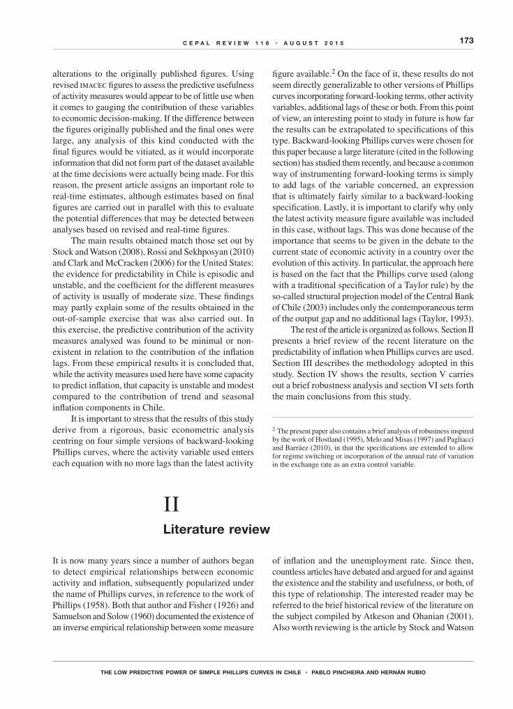
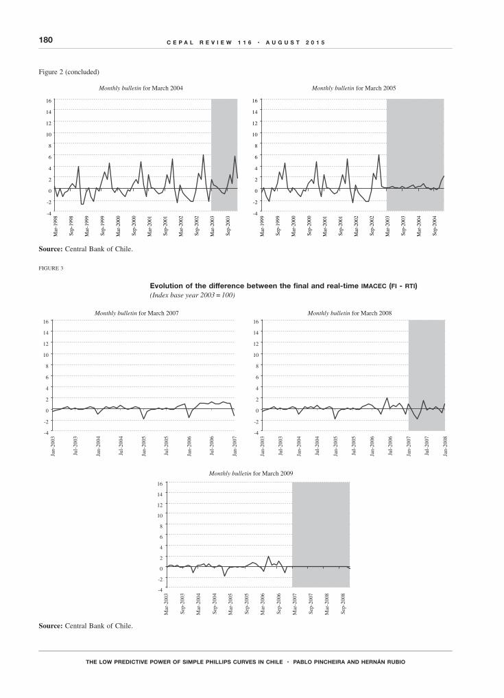
the latest figure will be a preliminary one, but it is also likely that the penultimate figure in the series will be on its second revision, and that the figure for December 2008 will be on its third or fourth revision. Again, the figure for December 2000 will probably be final. Thus, economic agents have to deal with heterogeneous time series, comprising a mix of final figures and figures that have been through different rounds of revision. An important question is whether this heterogeneity will result in some kind of noise or bias in the variables to be estimated. Morandé and Tejada (2008) answer this question affirmatively when calculating the output gap. This study will set out to evaluate differences in the ability of different activity measures to predict inflation. It will also seek to consider what differences there might potentially be in inflation forecasts as such. Nonetheless, before the issues of interest are directly evaluated in this way, it is advisable to carry out a graphic evaluation of whether the differences between real-time and final series are large. Figures 1 and 3 show sequences of time series illustrating the differences between those available in real time and those produced with final data. The panels of the charts differ in the base year taken to calculate the activity figures. Each panel within each chart represents the difference between the final imacec and the one published in the monthly bulletin of the Central Bank of Chile in March each year. These results are presented for a subsample of the period from 1997 to 2009. The shaded areas in the panels indicate that the values for that period include non-final data. What is calculated in these areas is the difference between the latest release available and the corresponding real-time figure.

Figure 1 analyses the curves only up to the month of December 1995. This is because from January 2006 onward there are no final imacec figures having 1986 as the base year, since subsequent rounds of revisions were carried out with 1996 as the base. To avoid comparing figures with different base years, it was considered preferable to focus on data available only up to December 1995. The first panel (with figures from the March 1996 monthly bulletin) shows a large revision between the real-time figures and the final ones. Consistently with the finding of Pincheira (2010), the final figures show the real-time ones to be significant underestimates, and the fewer rounds of revision they have been through, the larger the underestimate. The same pattern can be seen in the second panel of figure 1. Nonetheless, the next two panels show that there were virtually no revisions

in the publications of March 1998 onward for figures prior to January 1996. This indicates that the figures for December 1995 and earlier had been practically finalized by March 1998.

Figure 2 shows a very different situation to figure 1. It should be recalled that figure 2 compares series whose base year is 1996. For the reasons indicated in the previous paragraph, only figures up to December 2002 will be compared, since final imacec figures with base year 1996 are available up to that date. The four panels of figure 2 are very different to those of figure 1. First, there were continual revisions during the five years of evolution encompassed by figure 2, since all the panels show discrepancies between the final and real-time series. Second, the pattern of revisions in each panel is different to the one in the first panel of figure 1. There is no longer an upward trend in the panels, or such a strong bias towards underestimation relative to the final imacec as in figure 1. It is also striking that the revisions shown in figure 2 are medium-sized and present something of a seasonal pattern.

Figure 3 compares series constructed using base year 2003. Only the period between January 2003 and December 2006 is analysed. This period is chosen because data with base year 2003 are only available from January that year and because the latest finalized data are assumed to be those for December 2006.

The behaviour of revisions in figure 3 is different from that in figures 1 and 2; they are smaller and have a considerably less marked seasonal pattern than in figure 2.

The results of figures 1, 2 and 3 form an interesting picture where revisions follow very different processes, with size and bias tending to diminish over time, something that is wholly consistent with the analogous result shown by Pincheira (2010) for annual gdp growth. If the revision process continues to show this tendency towards diminishing size and bias, the uncertainty resulting from the non-availability of definitive real-time data will unquestionably tend to ease and perhaps disappear. Nonetheless, the same analysis carried out here suggests that this source of uncertainty has been considerable in the sample dealt with by the present study.8

8 To put a different perspective on the current size of revisions, the differences between the real-time and revised series were also calculated as 12-month changes. In some months, the differences between the two series exceeded 200 basis points, showing the size of revisions to be substantial.



FIGURE 1

Evolution of the difference between the final and real-time imacec (fi - rti) (Index base year 1986 = 100)

-4

-2

0

2

4

6

8

10

12

14

16

Mar

-199

0

Sep-

1990

Mar

-199

1

Sep-

1991

Mar

-199

2

Sep-

1992

Mar

-199

3

Sep-

1993

Mar

-199

4

Sep-

1994

Mar

-199

5

Sep-

1995

-4

-2

0

2

4

6

8

10

12

14

16

Mar

-199

1

Sep-

1991

Mar

-199

2

Sep-

1992

Mar

-199

3

Sep-

1993

Mar

-199

4

Sep-

1994

Mar

-199

5

Sep-

1995

Mar

-199

6

Sep-

1996

-4

-2

0

2

4

6

8

10

12

14

16

Mar

-199

2

Sep-

1992

Mar

-199

3

Sep-

1993

Mar

-199

4

Sep-

1994

Mar

-199

5

Sep-

1995

Mar

-199

6

Sep-

1996

Mar

-199

7

Sep-

1997

-4

-2

0

2

4

6

8

10

12

14

16 M

ar-1

993

Sep-

1993

Mar

-199

4

Sep-

1994

Mar

-199

5

Sep-

1995

Mar

-199

6

Sep-

1996

Mar

-199

7

Sep-

1997

Mar

-199

8

Sep-

1998

Monthly bulletin for March 1996 Monthly bulletin for March 1997


Source: Central Bank of Chile.

FIGURE 2


-4

-2

0

2

4

6

8

10

12

14

16

Mar

-199

6

Sep-

1996

Mar

-199

7

Sep-

1997

Mar

-199

8

Sep-

1998

Mar

-199

9

Sep-

1999

Mar

-200

0

Sep-

2000

Mar

-200

1

Sep-

2001

-4

-2

0

2

4

6

8

10

12

14

16

Mar

-199

7

Sep-

1997

Mar

-199

8

Sep-

1998

Mar

-199

9

Sep-

1999

Mar

-200

0

Sep-

2000

Mar

-200

1

Sep-

2001

Mar

-200

2

Sep-

2002

-4

-2

0

2

4

6

8

10

12

14

16

Mar

-199

8

Sep-

1998

Mar

-199

9

Sep-

1999

Mar

-200

0

Sep-

2000

Mar

-200

1

Sep-

2001

Mar

-200

2

Sep-

2002

Mar

-200

3

Sep-

2003

-4

-2

0

2

4

6

8

10

12

14

16

Mar

-199

9

Sep-

1999

Mar

-200

0

Sep-

2000

Mar

-200

1

Sep-

2001

Mar

-200

2

Sep-

2002

Mar

-200

3

Sep-

2003

Mar

-200

4

Sep-

2004





FIGURE 3


-4

-2

0

2

4

6

8

10

12

14

16

Jan-

2003

Jul-

2003

Jan-

2004

Jul-

2004

Jan-

2005

Jul-

2005

Jan-

2006

Jul-

2006

Jan-

2007

-4

-2

0

2

4

6

8

10

12

14

16

Jan-

2003

Jul-

2003

Jan-

2004

Jul-

2004

Jan-

2005

Jul-

2005

Jan-

2006

Jul-

2006

Jan-

2007

Jul-

2007

Jan-

2008

-4

-2

0

2

4

6

8

10

12

14

16

Mar

-200

3

Sep-

2003

Mar

-200

4

Sep-

2004

Mar

-200

5

Sep-

2005

Mar

-200

6

Sep-

2006

Mar

-200

7

Sep-

2007

Mar

-200

8

Sep-

2008


Monthly bulletin for March 2009


-4

-2

0

2

4

6

8

10

12

14

16

Mar

-199

6

Sep-

1996

Mar

-199

7

Sep-

1997

Mar

-199

8

Sep-

1998

Mar

-199

9

Sep-

1999

Mar

-200

0

Sep-

2000

Mar

-200

1

Sep-

2001

-4

-2

0

2

4

6

8

10

12

14

16

Mar

-199

7

Sep-

1997

Mar

-199

8

Sep-

1998

Mar

-199

9

Sep-

1999

Mar

-200

0

Sep-

2000

Mar

-200

1

Sep-

2001

Mar

-200

2

Sep-

2002

-4

-2

0

2

4

6

8

10

12

14

16

Mar

-199

8

Sep-

1998

Mar

-199

9

Sep-

1999

Mar

-200

0

Sep-

2000

Mar

-200

1

Sep-

2001

Mar

-200

2

Sep-

2002

Mar

-200

3

Sep-

2003

-4

-2

0

2

4

6

8

10

12

14

16

Mar

-199

9

Sep-

1999

Mar

-200

0

Sep-

2000

Mar

-200

1

Sep-

2001

Mar

-200

2

Sep-

2002

Mar

-200

3

Sep-

2003

Mar

-200

4

Sep-

2004




Figure 2 (concluded)



2. In-sample predictive evaluation: revised data

The first exercise carried out here consists in estimating equations (1) to (4) in 152 rolling windows of 71 observations each to get an idea of the evolution of the g parameter for each activity measure taken. The first window captures the monthly imacec data between January 1991 and November 1996. This first exercise is carried out with revised data available on the website of the Central Bank of Chile as of 2009. Even so, the imacec series has been seasonally adjusted and the output gap calculated using the Hodrick-Prescott filter in each estimation window, to avoid incorporating future information into the estimates. The assumption has been that the latest figure which will not undergo further revision is that for December 2006. Accordingly, the charts that follow are shaded from January 2007 onward to indicate that the values from that month include non-final data. Each model is estimated with eight variants. These variants take different numbers of inflation lags (from 1 to 4 lags), plus inclusion or exclusion of the “inflation target” variable. A robust estimate of the γ parameter is obtained by taking the Bayesian average for the eight variants of each model considered. To this end, the expressions shown in annex C of Pincheira and Calani (2010) are employed on the basis of heteroskedasticity and autocorrelation consistent (hac) estimates of the variances of the individual parameters of each model in according with the method of Newey and West (1987 and 1994). Also calculated are variances that are robust to model uncertainty in accordance with Bayesian averaging, and in this way asymptotically normal t-type statistics are constructed. The evolution of the γ parameter in models 1 and 3 for horizons of 1, 3, 6, 9 and 12 months, and that of its p values, can be seen in figures 4 and 5.

The thicker curve represents the robust estimate of the γ parameter associated with the activity variable being used. The thin line indicates the p value associated with the coefficient. The dotted straight line marks the 10% significance level. This means that the parameter estimated will be statistically significant, with a confidence level of 90% or more, whenever the thin line is below the dotted straight line. Graphs of the γ parameter for models 2 and 4 are omitted because they are very similar to those of figure 4 and do not add any information substantially different to that already shown.

Perhaps the most interesting thing about all the charts is that they show an “episodic” statistical significance for the parameter associated with the activity variable. In other words, the statistical significance of this parameter varies over time so that periods of high significance are

followed by periods of low significance. Furthermore, this alternation tends to occur repeatedly during the sample period. The only exception to this frequent alternation is seen in model 3, where the oscillation in statistical significance is considerably smaller. Table 1 illustrates the “episodic” character of the parameter associated with the activity variable by showing the percentage of estimation windows where this parameter is significant at 10%. It can be seen that this percentage varies depending on the model and the prediction horizon taken. In particular, it can be seen that the greatest frequency of statistical significance is concentrated at the prediction horizon of one month for all the models. This frequency oscillates between 57.9% and 84.2%. Conversely, the lowest frequency of significance is concentrated at the longer prediction horizons of 9 and 12 months. With those horizons, the activity variable is found to be statistically significant in less than half the rolling estimation windows. When the behaviour of the models is compared, what is striking is that the results of specifications 1 and 2 are very similar. Model 3, meanwhile, is distinguished by having the lowest frequency of significance at the first two horizons. In turn, model 4 is distinguished by having the highest frequency of significance in month-ahead projections and the lowest frequencies at horizons of 6, 9 and 12 months ahead.

TABLE 1

Rolling windows where the parameter associated with economic activity is significant at 10%a

(Percentages)

Model 1 Model 2 Model 3 Model 4

h = 1 73.0 71.1 57.9 84.2h = 3 50.0 52.6 43.4 44.1h = 6 46.1 46.7 41.4 17.1h = 9 36.2 34.2 33.6 16.4h = 12 44.1 42.8 35.5 15.1

Source: Prepared by the authors.a Final data: January 1991 to June 2009.

Lastly, it is also important to mention the size of the γ parameter estimate. It is seen that, in general, the estimate for γ has a moderate or small value. Although its largest positive value in all the charts is 1.34, not a negligible figure, the average for the estimates obtained in all the rolling windows, for each model and horizon, is no more than 0.23. These numbers, plus visual inspection of figures 4 and 5, suggest that the predictive contribution of the activity variable in equations (1) to (4) is moderate and unstable.



All this goes to form a situation where the coefficient associated with the activity variable is, in general, “episodic” in terms of statistical significance, and where the estimator of this parameter presents instability and is of moderate size. These results are consistent with the hypothesis attributed to Michael McCracken, presented in

the Introduction, and also with those results for the United States where no greater predictability was found with a series of Phillips curves. In particular, this result is very similar to that reported by Stock and Watson (2008), insofar as the predictability provided by the versions of Phillips curves analysed so far can also be described as “episodic.”

FIGURE 4

Evolution of the parameter and p-value associated with economic activity in the Phillips curve of model 1, 1997-2009(Final data)

0

10

20

30

40

50

60

70

80

-0.05

0.00

0.05

0.10

0.15

0.20

0.25

0.30

0.35

1997

1998

1999

2000

2001

2002

2003

2004

2005

2006

2007

2008

2009

Gamma p-value (%) Signi�cance at 10%

-20

-10

0

10

20

30

40

50

60

70

-0.05

0.00

0.05

0.10

0.15

0.20

0.25

0.30

0.35

0.40

1997

1998

1999

2000

2001

2002

2003

2004

2005

2006

2007

2008

2009


-10

0

10

20

30

40

50

60

70

80

90

-0.10

0.00

0.10

0.20

0.30

0.40

0.50

0.60

0.70

0.80

0.90

1997

1998

1999

2000

2001

2002

2003

2004

2005

2006

2007

2008

2009


-80

-60

-40

-20

0

20

40

60

80

100

-0.40

-0.20

0.00

0.20

0.40

0.60

0.80

1.00

1.20

1.40

1997

1998

1999

2000

2001

2002

2003

2004

2005

2006

2007

2008

2009


0

20

40

60

80

100

120

-1.50

-1.00

-0.50

0.00

0.50

1.00

1.50

1997

1998

1999

2000

2001

2002

2003

2004

2005

2006

2007

2008

2009


Perc

enta

ge

Perc

enta

ge

Perc

enta

ge

Perc

enta

ge

Perc

enta

ge

Horizon 1 Horizon 3

Horizon 6 Horizon 9

Horizon 12

Source: Prepared by the authors.



FIGURE 5

Evolution of the parameter and p-value associated with economic activity in the Phillips curve of model 3, 1997-2009(Final data)

-80

-60

-40

-20

0

20

40

60

80

100

120

-0.08

-0.06

-0.04

-0.02

0.00

0.02

0.04

0.06

0.08

0.10

0.12

1997

1998

1999

2000

2001

2002

2003

2004

2005

2006

2007

2008

2009


-150

-125

-100

-75

-50

-25

0

25

50

75

100

-0.30

-0.25

-0.20

-0.15

-0.10

-0.05

0.00

0.05

0.10

0.15

0.20

1997

1998

1999

2000

2001

2002

2003

2004

2005

2006

2007

2008

2009


-60

-40

-20

0

20

40

60

80

100

-0.15

-0.10

-0.05

0.00

0.05

0.10

0.15

0.20

0.25

1997

1998

1999

2000

2001

2002

2003

2004

2005

2006

2007

2008

2009


-100

-75

-50

-25

0

25

50

75

100

-0.60

-0.40

-0.20

0.00

0.20

0.40

0.60

0.80

1.00 19

97

1998

1999

2000

2001

2002

2003

2004

2005

2006

2007

2008

2009


-90

-60

-30

0

30

60

90

120

-0.60

-0.40

-0.20

0.00

0.20

0.40

0.60

0.80

1997

1998

1999

2000

2001

2002

2003

2004

2005

2006

2007

2008

2009


Perc

enta

ge

Perc

enta

ge

Perc

enta

ge

Perc

enta

ge

Perc

enta

ge

Horizon 1 Horizon 3

Horizon 6 Horizon 9

Horizon 12




3. In-sample predictive evaluation: real-time data

The analysis carried out in this subsection is analogous to the one in the previous subsection, with the one great difference that this time the estimates are produced and the activity variable constructed with real-time data. This is done to assess whether the activity variables in the models (1 to 4) are useful for generating good inflation forecasts that can be employed by those required to take real-time decisions.

As in the analysis with revised data, figures 6 and 7 show “episodic” statistical significance for the parameter associated with the activity variable in models 1 and 3. The γ parameter is not charted for models 2 and 4 because the graphs are very similar to those of model 1 and do not add any information substantially different to that already shown. Table 2 is analogous to table 1 in that it shows the percentage of estimation windows in which this parameter is significant at 10%.

TABLE 2

Rolling windows where the parameter associated with economic activity is significant at 10%(Real-time data)


H = 1 65.8 65.1 73.0 73.0H = 3 65.8 63.8 44.7 56.6H = 6 63.2 60.5 39.5 39.5H = 9 53.9 55.3 38.2 35.5H = 12 48.7 50.0 40.8 28.9


What stands out is that this percentage varies depending on the model and the prediction horizon taken, much as happened when final data were used. In particular, the highest frequency of statistical significance is once again found to be concentrated at the prediction horizon of one month for all the models. This frequency oscillates between 65.1% and 73%. Conversely, the lowest frequency of significance is once again concentrated at the longer prediction horizons of 9 and 12 months. At those horizons, the activity variable is found to be statistically significant in at most 55.3% of the rolling estimation windows. When the behaviour of the models is compared, it also transpires that the results of specifications (1) and (2) are very similar. Model 3, meanwhile, is no

longer distinguished by having the lowest frequency of significance at the first two horizons; in fact, it shares first place with model 4 for the frequency of statistical significance at the one-month horizon. Model 4 is also distinguished by having the lowest frequency of significance at horizons of 9 and 12 months.

Where the size of the γ parameter estimate is concerned, the results are also similar to those obtained with final data. In fact, figures 6 and 7 reveal a small or moderate γ estimation value, peaking at 1.25 but averaging out to a value of no more than 0.30 across the estimates obtained in all the rolling windows. These figures, plus visual inspection of figures 6 and 7, suggest that the predictive contribution of the activity variable in equations (1) to (4) is moderate and unstable when this variable is introduced with real-time data, in a result very similar to that obtained with final data.

What has been carried out so far is a general or global comparison between the results associated with the activity parameter in equations (1) to (4), when this estimation is conducted with final and real-time data. There have been found to be a number of general similarities between these two estimates. However, this should not be taken as affirming that the nature of the data used to estimate specifications (1) to (4) is irrelevant. In fact, there can be substantial differences in both the γ estimates and the inflation forecasts yielded by a single equation estimated in the same sample period but with real-time or final data. This is seen in figures 8 and 9, which show that for certain periods the γ parameter estimate and the 12-month inflation projections derived from equations (1) to (4) look very different depending on whether estimation is carried out with real-time or final data. Indeed, differences in inflation forecasts have on occasion exceeded 100 basis points, and it is quite common to see differences of 50 basis points or so, which, while not enormous, do not seem negligible either.

In summary, this analysis suggests that, on average, the marginal contribution of the activity variable to inflation forecasting is episodic, moderate in size and unstable over time. This conclusion is robust to the nature of the data used to estimate the Phillips curves in this study. Nonetheless, individual inflation forecasts, and likewise each estimation of the parameter accompanying the activity variable, can change significantly depending on whether the equation concerned is estimated with revised data or in real time.



FIGURE 6

Real-time evolution of the parameter and p-value associated with economic activity in the Phillips curve of model 1a

(Percentages)

0

20

40

60

80

-0.02

0.03

0.08

0.13

0.18

1997

1998

1999

2000

2001

2002

2003

2004

2005

2006

2007

2008

2009


-20

0

20

40

60

-0.20

0.00

0.20

0.40

0.60

1997

1998

1999

2000

2001

2002

2003

2004

2005

2006

2007

2008

2009


0

20

40

60

80

100

0.00

0.20

0.40

0.60

0.80

1.00

1997

1998

1999

2000

2001

2002

2003

2004

2005

2006

2007

2008

2009


0

20

40

60

80

-0.40

0.10

0.60

1.10

1.60

1997

1998

1999

2000

2001

2002

2003

2004

2005

2006

2007

2008

2009


-20

0

20

40

60

80

100

-0.20

0.00

0.20

0.40

0.60

0.80

1.00

1997

1998

1999

2000

2001

2002

2003

2004

2005

2006

2007

2008

2009


Perc

enta

ge

Perc

enta

ge

Perc

enta

ge

Perc

enta

ge

Perc

enta

ge

Horizon 1 Horizon 3

Horizon 6 Horizon 9

Horizon 12

Source: Prepared by the authors.a Data from January 1991 to June 2009.



FIGURE 7

Real-time evolution of the parameter and p-value associated with economic activity in the Phillips curve of model 3(Real-time data)

0

20

40

60

80

-0.10

-0.05

0.00

0.05

0.10

0.15

1997

1998

1999

2000

2001

2002

2003

2004

2005

2006

2007

2008

2009

Gamma p-value (%) Signi�cance at10%

0

20

40

60

80

100

-0.20

-0.15

-0.10

-0.05

0.00

0.05

0.10

0.15

0.20

0.25

1997

1998

1999

2000

2001

2002

2003

2004

2005

2006

2007

2008

2009


0

20

40

60

80

-0.30

-0.20

-0.10

0.00

0.10

0.20

0.30

0.40

0.50

0.60

1997

1998

1999

2000

2001

2002

2003

2004

2005

2006

2007

2008

2009


0

20

40

60

80

100

-0.50

-0.25

0.00

0.25

0.50

0.75

1997

1998

1999

2000

2001

2002

2003

2004

2005

2006

2007

2008

2009


0

20

40

60

80

100

-0.60

-0.30

0.00

0.30

0.60

0.90

1997

1998

1999

2000

2001

2002

2003

2004

2005

2006

2007

2008

2009


100

100

Perc

enta

ge

Perc

enta

ge

Perc

enta

ge

Perc

enta

ge

Perc

enta

ge

Horizon 1 Horizon 3

Horizon 6 Horizon 9

Horizon 12




FIGURE 8

Difference between γ estimates in the same equation estimated with final and real-time data

-0.5

-0.4

-0.3

-0.2

-0.1

0

0.1

0.2

0.3

0.4

0.5

Jan1997

Jan1998

Jan1999

Jan2000

Jan2001

Jan2002

Jan2003

Jan2004

Jan2005

Jan2006

Jan2007

Jan2008

Jan2009



FIGURE 9

Difference between the 12-month inflation forecasts of the same equation estimated with final and real-time data

-1.75

-1.5

-1.25

-1

-0.75

-0.5

-0.25

0

0.25

0.5

0.75


Nov

-199

7

Jul-

1998

Mar

-199

8

Nov

-200

3

Jul-

2004

Mar

-200

4

Nov

-200

4

Jul-

2005

Mar

-200

5

Nov

-200

5

Jul-

2006

Mar

-200

6

Nov

-200

6

Jul-

2007

Mar

-200

7

Nov

-200

7

Jul-

2008

Mar

-200

8

Nov

-200

8

Mar

-200

9

Nov

-199

8

Jul-

1999

Mar

-199

9

Nov

-199

9

Jul-

2000

Mar

-200

0

Nov

-200

0

Jul-

2001

Mar

-200

1

Nov

-200

1

Jul-

2002

Mar

-200

2

Nov

-200

2

Jul-

2003

Mar

-200

3




4. Complementary out-of-sample results

The results presented in the previous subsections were simple in-sample regressions. The “episodic” and unstable character of the estimator for the coefficient associated with the economic activity variable, and its moderate size, are an indication that in out-of-sample prediction exercises, the predictive contribution of economic activity measures should be minimal. Table 3 bears this out. The table shows the ratio of the root mean squared error for out-of-sample projection of each of the models (1 to 4), estimated with and without the activity variable over the five horizons that have been taken in this study: 1, 3, 6, 9 and 12 months ahead. The predictive exercise employs the same rolling windows of 71 observations as were used for the in-sample analysis. It should be noted that specifications with four lags for inflation were taken for this stage. Most of the figures in table 3 are found to be less than 1, an indication that including the activity variable impairs the predictive accuracy of the models in most cases. This is consistent with the instability detected in the parameters associated with the activity variable, its “episodic” character and its moderate size.

Table 4 supplements this analysis, comparing the root mean squared error of the Phillips curves with a prototype model proposed by Stock and Watson (2008) (see the annex for more details) and some simple time series models.9 It can be seen that the forecasts from the Phillips curves are less accurate than the best time series models taken over all horizons. Also interesting to highlight is that the difference in predictive accuracy between the models estimated with revised and real-time

9 The time series models considered are a random walk with constant and two sarima models similar to the airline model of Box and Jenkins (1970). These sarima models are described in great detail in Pincheira and García (2009) and in Pincheira and Medel (2015), with these studies also showing their excellent predictive capacity for inflation in Chile and a select group of countries. A brief summary with the sarima specifications used in this document can be found in the annex.

data is very small, something that is consistent with the minimal contribution usually made by the activity variables considered here, whose inclusion is actually detrimental in many cases.

There are two further observations about statistical inference exercises that the authors of the present article consider worth highlighting. First, it would appear that the application of predictive ability tests of the type used by Diebold and Mariano (1995), West (1996) and Giacomini and White (2006) does not constitute a major contribution for the purposes of this study, basically because the mean squared errors yielded by the models (1 to 4) have usually been found to be lower when they are estimated without the activity variable, ensuring that these tests cannot reject the null hypothesis of equal predictive ability in favour of the models that include activity variables. In other words, at worst, the null hypothesis cannot be rejected. While it is true that activity variables do reduce the root mean squared error in a few cases, the reduction is never greater than 2%. Even if reductions of this size were statistically significant, it would be hard to argue that they were economically significant, and there seems to be no point in implementing inference exercises considered unlikely a priori to be able to contribute significantly to the conclusions of this study.

Second, as discussed in Clark and West (2006 and 2007) and Pincheira (2013), this comparison of mean squared errors would not necessarily imply that the activity variables had no contribution to make to predicting inflation. This is because comparing mean squared errors between nested models usually favours the model with fewest parameters to be estimated. In this paper, however, not only has a mean squared error calculation been carried out, but the unstable and moderate predictive contribution of the activity variables has been seen in in-sample regressions too. In summary, both the in-sample and out-of-sample analyses indicate a weak contribution by the activity variables to the prediction of inflation, at least in the context of the models (1 to 4) used here.



TABLE 3

Ratio of the root mean squared error in inflation projections with and without the activity variable a

(A value of less than 1 favours the specification without the activity variable)

Horizon

h = 1 h = 3 h = 6 h = 9 h = 12

Model 1 Real-time no target 0.98 0.94 0.93 0.90 0.97target 0.98 0.94 0.92 0.89 0.96

Corrected no target 0.97 0.95 0.94 0.90 0.96target 0.97 0.95 0.94 0.90 0.94







Source: Prepared by the authors.a Out-of-sample exercise between November 1997 and June 2009.

TABLE 4

Root mean squared error in inflation projectionsa

(Hundredths of a basis point)

Horizon

h = 1 h = 3 h = 6 h = 9 h = 12

Random walk with constant 0.48 1.04 1.75 2.20 2.53sarima with constant 0.35 0.90 1.50 1.81 2.00sarima with constant and autoregressive term 0.34 0.90 1.51 1.82 2.01Stock-Watson with constant 0.39 1.04 1.79 2.26 2.55Stock-Watson without constant 0.39 1.03 1.73 2.18 2.45Phillips 1 with final activity 0.44 1.00 1.79 2.39 2.48Phillips 1 with real-time activity 0.44 1.01 1.81 2.40 2.43Phillips 2 with final activity 0.44 0.99 1.78 2.37 2.47Phillips 2 with real-time activity 0.44 1.00 1.81 2.39 2.44Phillips 3 with final activity 0.45 1.00 1.72 2.24 2.49Phillips 3 with real-time activity 0.44 1.01 1.75 2.24 2.38Phillips 4 with final activity 0.47 0.99 1.78 2.17 2.25Phillips 4 with real-time activity 0.47 0.99 1.79 2.17 2.23

Source: Prepared by the authors.a Out-of-sample exercise between November 1997 and June 2009.



1. Models including regime switching

As stated earlier, the goal of the present study is to assess whether certain measures of economic activity have the capacity to predict inflation in the context of simple backward-looking versions of Phillips curves, following in the wake of a fairly recent international literature exemplified in the studies of Stock and Watson (2008), Rossi and Sekhposyan (2010), Clark and McCracken (2006) and Ciccarelli and Mojon (2010).

Notwithstanding the above, it is clear that there are innumerable alternative specifications for predicting inflation, even within the category of Phillips curves itself. A line of research parallel to the one followed here has focused on using Markov regime switching models to characterize inflation. Examples of this include the studies by Hostland (1995), Melo and Misas (1997), Amisano and Fagan (2013) and Pagliacci and Barráez (2010). Of these, the closest to the present article are Pagliacci and Barráez (2010) and Amisano and Fagan (2013).

A cursory robustness analysis entails the employment of in-sample estimations of backward-looking Phillips curves, like those specified in this study, but with the option of endogenous regime switching along the lines of Hamilton (1989), in accordance with the following specifications:

RS1 model:

Y Y

, ,

*

is

t i t hi

n

t hs

ts s

t t

1 10

1 1 1 1 1

{ r f

r d r a c

+ +

= + + −

- +=

+ - -` j/ , s = 1,2

RS2 model:

ln lnY Y100 *

, ,

t t

is

t i t hi

n

t hs

ts s

1 1

0

2 2 2

2 2{ r f

r d r a c

+ +

= + + −- -

- +=

+ b l7 9A C/ , s = 1,2

RS3 model:

ln lnY Y100

, ,

t t

is

t i t hi

n

t hs

ts s

1 13

0

3 3 3

3 3{ r f

r d r a c

+ +

= + + −- -

- +=

+ ` j7 7A A/ , s = 1,2

RS4 model:

ln lnY Y100 *

, ,

t t

is

t i t hi

n

t h ts

ts s

1 1

0

4 4 4

4 4{ r f

r r d r a c

+ +

− = + + −- -

- +=

+ b l7 9A C/ , s = 1,2

These alternative specifications are a generalization of the original expressions (1) to (4), but allowing for two regimes for inflation.

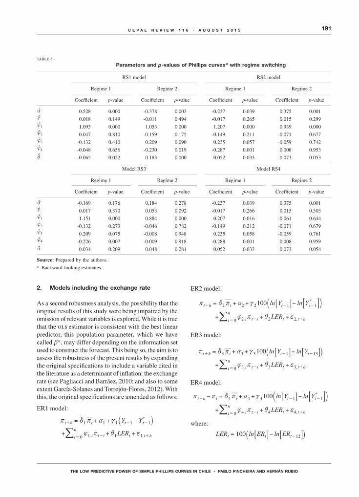
Table 5 presents the results of the estimates when forecasting a month ahead. Exogenously incorporated into them is the possibility that two different regimes exist, differentiated by subscript s. The coefficient of the activity term is found to be small in all the specifications. Furthermore, only in the rs3 model is the activity variable found to have a statistically significant coefficient, something that occurs in regime 2. There is no statistical significance in any of the other cases. Generally speaking, in other words, the results are similar to those from the linear specifications: the activity terms only have an episodic predictive capacity. Interestingly, table 5 also provides a basis for conjecture about the characteristics that seem to differentiate one regime from the other. One regime appears to be characterized by a unit root, or at least by a process with a root close to 1, while the other seems to have considerably lower persistence. In any event, this is only a conjecture that would be worth evaluating in greater depth in future studies. The authors of the present study also think that it would be valuable to investigate the predictive out-of-sample behaviour of regime switching models, and this is likewise suggested for a future research agenda.

VA brief robustness analysis



TABLE 5

Parameters and p-values of Phillips curves a with regime switching

RS1 model RS2 model

Regime 1 Regime 2 Regime 1 Regime 2

Coefficient p-value Coefficient p-value Coefficient p-value Coefficient p-value

at 0.528 0.000 -0.378 0.003 -0.237 0.039 0.375 0.001ct 0.018 0.149 -0.011 0.494 -0.017 0.265 0.015 0.299

1{t 1.093 0.000 1.053 0.000 1.207 0.000 0.939 0.0002{t 0.047 0.810 -0.159 0.175 -0.149 0.211 -0.071 0.6773{t -0.132 0.410 0.209 0.090 0.235 0.057 -0.059 0.7424{t -0.048 0.656 -0.230 0.019 -0.287 0.001 0.008 0.953

dt -0.065 0.022 0.183 0.000 0.052 0.033 0.073 0.053

Model RS3 Model RS4

Regime 1 Regime 2 Regime 1 Regime 2

Coefficient p-value Coefficient p-value Coefficient p-value Coefficient p-value

at -0.169 0.176 0.184 0.278 -0.237 0.039 0.375 0.001ct 0.017 0.370 0.053 0.092 -0.017 0.266 0.015 0.303

1{t 1.151 0.000 0.884 0.000 0.207 0.016 -0.061 0.6442{t -0.132 0.273 -0.046 0.782 -0.149 0.212 -0.071 0.6793{t 0.209 0.075 -0.008 0.948 0.235 0.058 -0.059 0.7614{t -0.226 0.007 -0.009 0.918 -0.288 0.001 0.008 0.959

dt 0.034 0.209 0.048 0.281 0.052 0.033 0.073 0.054

Source: Prepared by the authors.a Backward-looking estimates.

2. Models including the exchange rate

As a second robustness analysis, the possibility that the original results of this study were being impaired by the omission of relevant variables is explored. While it is true that the ols estimator is consistent with the best linear predictor, this population parameter, which we have called b*, may differ depending on the information set used to construct the forecast. This being so, the aim is to assess the robustness of the present results by expanding the original specifications to include a variable cited in the literature as a determinant of inflation: the exchange rate (see Pagliacci and Barráez, 2010; and also to some extent García-Solanes and Torrejón-Flores, 2012). With this, the original specifications are amended as follows:

ER1 model:

i f+ +- +

Y Y

LER

*

, ,

t h t t t

i t i t t hi

n

1 1 1 1 1

1 1 10

r d r a c

{ r

= + + −

+

+ - -

=

` j/

ER2 model:

i f+ +- +

ln lnY Y

LER

100 *

, ,

t h t t t

i t i t t hi

n

1 1

0

2 2 2

2 2 2

r d r a c

{ r

= + + −

+

+ - -

=

b l7 9A C/

ER3 model:

i f- ++ +

ln lnY

LER

Y100

, ,

t h t t

i t i t t hi

n

t1

0

3 3 3

3 3 3

13r d r a c

{ r

= + + −

+

+ -

=

-` j7 7A A/

ER4 model:

i f- ++ +

ln lnY Y100

, ,

*t h t t t

i t i t t hi

n

t1

0

4 4 4

4 4 4

1r r d r a c

{ r

− = + + −

+

+ -

=

-b l7 9A C/ LER

where:

A At t= −7 7ln ln100 t 12-` jLER ER ER



while ert represents the observed exchange rate (Chilean pesos per United States dollar) reported by the Central Bank of Chile.

Thus, the aim is to analyse whether the episodic character of the parameters associated with the activity variables is altered or not when the annual rate of variation in the exchange rate is included as an additional predictor. To this end, the above equations are estimated in the same rolling windows as reported in section IV.2. Table 6 shows the percentage of these windows where the parameter associated with activity proved statistically significant with a confidence level of 90%. In other words, table 6 is analogous to table 1 above.

As can be seen in table 6, the episodic character of the parameter associated with the activity variable is maintained. It is clear that the percentage of windows where this parameter is statistically significant fluctuates between 11.8% and 64.5%. The general average of the percentages is 39.2% in table 6, while in table 1 it is 44.3%. In summary, incorporating the exchange rate as an additional predictor is not found to qualitatively alter the results. It could even be argued that including

the exchange rate diminishes the predictive capacity of activity, but on the whole, comparison of tables 1 and 6 shows that the results are dependent on the specification. In equations (1), (2) and (4), including the exchange rate somewhat diminishes the statistical significance of the activity variable parameter, while in specification (3) there is the opposite tendency.

TABLE 6

Rolling windows where the parameter associated with economic activity is significant at 10%a

(Percentages)

ER1 model

ER2 model

ER3 model

ER4 model

h = 1 50.0 50.0 64.5 57.9h = 3 46.7 46.1 41.4 28.3h = 6 40.1 40.8 56.6 11.8h = 9 23.0 23.7 55.9 17.8h = 12 30.9 28.3 44.1 25.7

Source: Prepared by the authors.a Final data: January 1991 to June 2009. Specifications with

exchange rate.

VISummary and conclusions

This study has considered four families of backward-looking Phillips curves for Chile with a monthly frequency and has assessed the capacity of these to predict inflation at horizons of 1, 3, 6, 9 and 12 months. All the specifications considered include an activity variable that is lagged relative to the latest inflation figure available, in order to emulate the availability of information in real time. It is done in this way because the imacec data used in this study to construct the activity variable are published with a month’s delay relative to the inflation figure. The predictability analysis is conducted both with revised figures and with figures available in real time, making it possible to evaluate the predictive economic relationship and the usefulness of these Phillips curves when it comes to generating projections for the use of decision makers.

The results obtained here indicate that the predictive capacity of these Phillips curves is limited and, furthermore, that the contribution made by the activity component to this predictability is moderate in size, often not

statistically significant, and fairly unstable. This holds true both for the real-time analysis and for the analysis with revised figures.

As a cursory analysis of robustness, the specifications were expanded to allow for the possibility of Markov-style regime switching, or the inclusion of the annual rate of variation in the exchange rate as an additional predictor. In-sample estimates of these expanded specifications are consistent with the results obtained in simpler linear specifications, since the statistical significance of the parameter associated with the activity variable continues to be occasional or episodic.

Part of the literature states that out-of-sample predictability assessments lack predictive power compared to in-sample assessments. It is for this reason that the present study has conducted exercises of both types, obtaining results that point in the same direction. Thus, it seems more plausible to attribute the lack of predictability to the unstable and moderate absolute



value of the coefficient associated with the respective activity variables than to problems with the predictive power of out-of-sample statistical tests.

Although the results of this study are consistent with those of a number of articles dealing with the United

States, they are novel in that they demonstrate a lack of predictive power for backward-looking Phillips curves in Chile. It will be part of a future agenda to determine whether these interesting results continue to obtain with other versions of Phillips curves.

ANNEX

Stock and Watson (2008) methodology

For many years, the Phillips curve has been heavily used as a tool for predicting inflation. However, the empirical results provided by this paper, and by a substantial section of the literature, are not necessarily satisfactory if the comparison is made with models where only past inflation is considered. Stock and Watson (2008) present a prototype autoregressive model with the following specification:

t hh

th

ih

t ii

n

t hh1 1

0

r r a z r fD− = ++ -=

+_ _ _ _ _ _i i i i i i/

where: ln lnh

P P1200

th

t t hr = − -_ __ i ii 9 C

is annualized inflation accumulated over h periods from time t; t

1r_ i is annualized inflation accumulated over just one month; the variable t h

hf +_ i represents shocks

uncorrelated with the information available at t; and ha_ i is a constant that can vary depending on the inflation accumulation period used.

The exercise proposed here consists in estimating this prototype model, with and without constant, in 152 rolling windows of 71 observations apiece. The first window takes cpi data from January 1991 to November 1996. A number of models are estimated in each window, taking different numbers of lags for the inflation differential

t i1rD -_ i (from 0 to 12 lags). The Schwarz criterion was

used to determine the best model within each window. Once the model had been selected, with the number of lags already determined for the independent variable, projections were carried out at different horizons: 1, 3,

6, 9 and 12 months ahead. Since the predictive results yielded by these models are a function of inflation, simple algebraic steps give a forecast at different horizons for the target variable, which is cumulative 12-month inflation. The out-of-sample root squared error obtained with this methodology is presented in table 4.

sarima models

Apart from the Stock and Watson models detailed earlier, the time series models considered in table 4 of this study are a random walk with constant and two sarima models similar to the airline model of Box and Jenkins (1970). These sarima models are described in great detail in Pincheira and García (2009) and Pincheira and Medel (2015), with these articles also demonstrating their excellent predictive capacity for inflation in Chile and a select group of countries. In particular, the three models used here have the following specifications:

Random walk with constant: t t t1r a r f= + +-

sarima 1: t t t t t1 12 13r a f if jf jif= + − − +- - -

sarima 2: t t t t

t t

1 1

12 13

r a tr f if

jf jif

= + + −

− +- -

- -

where: i i= −_ _ln lnCPI CPI100t t t 12r -9 C

The model denominated sarima 1 corresponds to the model denominated “sarima with constant” in table 4. The sarima 2 model corresponds to the model denominated “sarima with constant and autoregressive term”, again in table 4.



Amisano, G. and G. Fagan (2013), “Money growth and inflation: a regime switching approach”, Journal of International Money and Finance, vol. 33(C), Amsterdam, Elsevier.

Aguirre, A. and L.F. Céspedes (2004), “Uso de análisis factorial dinámico para proyecciones macroeconómicas”, Economía Chilena, vol. 7, No. 3, Santiago, Central Bank of Chile.

Atkeson, A. and L. Ohanian (2001), “Are Phillips curves useful for forecasting inflation?”, Quarterly Review, vol. 25, No. 1, Minneapolis, Federal Reserve Bank of Minneapolis.

Box, G. and G. Jenkins (1970), Time Series Analysis: Forecasting and Control, San Francisco, Holden-Day.

Box, G. and G. Tiao (1973), Bayesian Inference in Statistical Analysis, New York, John Wiley and Sons.

Brock, W. and S. Durlauf (2001), “Growth empirics and reality”, The World Bank Economic Review, vol. 15, No. 2, Washington, D.C., World Bank.

Central Bank of Chile (2003), Modelos macroeconómicos y proyecciones del Banco Central de Chile 2003, Santiago.

Céspedes, L.F., M. Ochoa and C. Soto (2005), “The new Keynesian Phillips curve in an emerging market economy: the case of Chile”, Documento de Trabajo, No. 355, Santiago, Central Bank of Chile.

Chih-Chuan, Yeh (2009), “The Simultaneous Evolution of Growth and Inflation”, document presented at the International Conference on Applied Economics.

Chumacero, R. and F. Gallego (2002), “Trends and cycles in real-time”, Estudios de Economía, vol. 29, No. 2, Santiago, University of Chile.

Ciccarelli, M. and B. Mojon (2010), “Global inflation”, The Review of Economics and Statistics, vol. 92, No. 3, Cambridge, Massachusetts, The mit Press.

Clark, T. and K. West (2007), “Approximately normal tests for equal predictive accuracy in nested models”, Journal of Econometrics, vol. 138, No. 1, Amsterdam, Elsevier.

(2006), “Using out-of-sample mean squared prediction errors to test the martingale difference hypothesis”, Journal of Econometrics, vol. 135, No. 1-2, Amsterdam, Elsevier.

Clark, T. and M. McCracken (2006), “The predictive content of the output-gap for inflation: Resolving in-sample and out-of-sample evidence”, Journal of Money, Credit and Banking, vol. 38, No. 5, Columbus, Ohio, The Ohio State University Press.

Diebold, F. and R. Mariano (1995), “Comparing predictive accuracy”, Journal of Business and Economic Statistics, vol. 13, No. 3, American Statistical Association.

Estrella A. and J. Fuhrer (2003), “Monetary policy shifts and the stability of monetary policy models”, Review of Economics and Statistics, vol. 85, No. 1, Cambridge, Massachusetts, The mit Press.

Fisher I. (1973), “I discovered the Phillips curve”, Journal of Political Economy, vol. 81, No. 2, Chicago, University of Chicago Press.

(1926), “A statistical relationship between unemployment and price changes”, International Labour Review, vol. 13, No. 6, International Labour Organization (ilo), June.

Fuentes, R., F. Gredig and M. Larraín (2008), “La brecha de producto en Chile: medición y evaluación”, Economía Chilena, vol. 11, No. 2, Santiago, Central Bank of Chile.

García, M. and J.P. Medina (2008), “Efectos de primas financieras sobre la actividad agregada”, Economía Chilena, vol. 12, No. 3, Santiago, Central Bank of Chile.

García-Solanes, J. and F. Torrejón-Flores (2012), “Inflation targeting works well in Latin America”, cepal Review, No. 106 (LC/G.2518-P), Santiago.

Giacomini, R. and H. White (2006), “Tests of conditional predictive ability”, Econometrica, vol. 74, No. 6, New York, The Econometric Society.

Hamilton, J. (1994), Time Series Analysis, Princeton, Princeton University Press.

(1989), “A new approach to the economic analysis of nonstationary time series and the business cycle”, Econometrica, vol. 57, No. 2, New York, The Econometric Society.

Hansen, B. (2014), “Econometrics”, University of Wisconsin, Madison, unpublished.

Hostland, D. (1995), “Changes in the inflation process in Canada: evidence and implications”, Working Paper, No. 1995-5, Ottawa, Bank of Canada.

Lansing, K. (2002), “Can the Phillips curve help forecast inflation”, frbsf Economic Letter, No. 29, San Francisco, Federal Reserve Bank of San Francisco.

Meese, R. and K. Rogoff (1983), “Empirical exchange rate models of the seventies. Do they fit out-of-sample?”, Journal of International Economics, vol. 14, No. 1-2, Amsterdam, Elsevier.

Melo, L. and M. Misas (1997), “Análisis del comportamiento de la inflación trimestral en Colombia bajo cambios de régimen: Una evidencia a través del modelo ‘Switching’ de Hamilton”, Borradores de Economía, No. 86, Bogota, Bank of the Republic of Colombia.

Morandé, F. and M. Tejada (2008), “Fuentes de incertidumbre monetaria en la conducción de la política monetaria en Chile”, Economía Chilena, vol. 11, No. 3, Santiago, Central Bank of Chile.

Nadal de Simone, F. (2001), “Proyección de la inflación en Chile”, Economía Chilena, vol. 4, No. 3, Santiago, Central Bank of Chile.

Newey, W. and K. West (1994), “Automatic lag selection in covariance matrix estimation”, Review of Economic Studies, vol. 61, No. 4, Wiley Blackwell.

(1987), “A simple, positive, semi-definite, heteroskedasticity and autocorrelation consistent covariance matrix”, Econometrica, vol. 55, No. 3, New York, The Econometric Society.

Pagliacci, C. and D. Barráez (2010), “A Markov-switching model of inflation: looking at the future during uncertain times”, Análisis Económico, vol. 25, No. 59, Autonomous Metropolitan University.

Pedersen, M. (2013), “Extracting gdp signals from the monthly indicator of economic activity. Evidence from Chilean real-time data”, Journal of Business Cycle Measurement and Analysis, vol. 2013(1), oecd Publishing.

Phillips, A. (1958), “The relation between unemployment and the rate of change in money wage rates in the United Kingdom, 1861-1957”, Economica, vol. 25, Wiley, November.

Pincheira P. (2013), “Shrinkage based tests of predictability”, Journal of Forecasting, vol. 32, No. 4, Wiley.

(2010), “A real time evaluation of the Central Bank of Chile gdp growth forecasts”, Money Affairs, vol. 23, No. 1, Center for Latin American Monetary Studies.

Pincheira, P. and M. Calani (2010), “Communicational bias in monetary policy: can words forecast deeds?”, Economia, vol. 11, No. 1, Latin American and Caribbean Economic Association.

Pincheira, P. and A. García (2009), “En búsqueda de un buen benchmark predictivo para la inflación”, Documento de Trabajo, No. 514, Santiago, Central Bank of Chile.

Pincheira, P. and C. Medel (2015), “Forecasting inflation with a simple and accurate benchmark: The case of the us and a set of inflation targeting countries”, Czech Journal of Economics and Finance, vol. 65, No. 1.

Rossi, B. and T. Sekhposyan (2010), “Have economic models’ forecasting performance for us output changed over time, and when?”, International Journal of Forecasting, vol. 26, No. 4, Amsterdam, Elsevier.

Rudebusch, G. and L. Svensson (1999), “Policy rules for inflation targeting”, Monetary Policy Rules, J.B. Taylor (ed.), Chicago, University of Chicago Press.

Russell, B. and R. Chowdhury (2013), “Estimating United States Phillips Curves with expectations consistent with the statistical process of inflation”, Journal of Macroeconomics, vol. 35, Amsterdam, Elsevier.

Samuelson, P. and R. Solow (1960), “Analytical aspects of anti-Inflation policy”, American Economic Review, vol. 50, No. 2, Nashville, Tennessee, American Economic Association.

Bibliography



Stock, J. and M. Watson (2008), “Phillips Curve inflation forecasts”, nber Working Paper, No. 14322, Cambridge, Massachusetts, National Bureau of Economic Research.

(1999), “Forecasting inflation”, Journal of Monetary Economics, vol. 44, No. 2, Amsterdam, Elsevier.

(1998), “Diffusion indexes”, nber Working Paper, No. 6702, Cambridge, Massachusetts, National Bureau of Economic Research.

Taylor, J.B. (1993), “Discretion versus policy rules in practice”, Carnegie-Rochester Conferences Series on Public Policy, vol. 39, No. 1, Amsterdam, Elsevier.

West, K. (2006), “Forecast evaluation”, Handbook of Economic Forecasting, G. Elliott, C.W.J. Granger and A. Timmerman (eds.), Amsterdam, Elsevier.

(1996), “Asymptotic inference about predictive ability”, Econometrica, vol. 64, No. 5, New York, The Econometric Society.

Yeh, C.C. (2009), “The Simultaneous Evolution of Growth and Inflation”, document presented at the International Conference on Applied Economics.

the low predictive power of simple phillips curves in chile

Documents