the journal of th - aqr capital management
TRANSCRIPT

Volume 21 No. 3 Winter 2018
“ Alternative strategies found their place in the investment universe once the industry addressed the difference between asset class and strategy, the appropriate assessment of their performance, and the impact of the different properties of return distributions on asset allocation processes.”
Jean Brunel
jwm.iprjournals.com
The Journalof
Wealth M
anagement
Winter 2
01
8, Volum
e 21
, No. 3
Nathan Sosner, Rodney Sullivan, and Liliana Urrutia
Multi-Period After-Tax Reporting: A Practical Solution
20thanniversary
P A R T T H R E E

The Journal of Wealth Management 3Winter 2018
NathaN SoSNer
is a managing director at AQR Capital Management in Greenwich, [email protected]
rodNey SullivaN
is a vice president at AQR Capital Management in Greenwich, [email protected]
liliaNa urrutia
is an associate at AQR Capital Management in Greenwich, [email protected]
Multi-Period After-Tax Reporting: A Practical SolutionNathaN SoSNer, rodNey SullivaN, aNd liliaNa urrutia
Effective, tax-aware investment management requires timely and informative after-tax performance reporting. While this is, perhaps,
an obvious statement, today such after-tax reporting remains largely absent while pre-tax performance reporting is widely avail-able and used. We are not the first to note this issue. In his article aptly titled “A Call to Arms! The Next Frontier for Taxable Accounts—After-Tax Return Performance Attribution,” Rogers (2005) emphasizes the importance of measuring and reporting tax-related information for taxable investors. He laments that, although a significant per-centage of the world’s invested assets are tax-able, only a miniscule fraction of managers employ after-tax reporting suitable for proper tax-aware management. Rogers points out that traditional performance reporting solu-tions that may work well for tax-exempt enti-ties such as retirement plans, charities, and endowments, fall short for taxable investors. Rogers concludes by inviting practitioners “to respond to ‘A Call to Arms’ and share with their peers possible solutions in an effort to conquer the after-tax performance attri-bution challenge.” Unfortunately, more than a decade later, despite such calls to action, consistent and useful after-tax performance reporting remains largely absent.1 Today,
1 In a survey of US-based CFA Institute mem-bers who manage private wealth, Horan and Adler
taxable investors typically receive pre-tax performance updates from their managers throughout the year, and only after the year is over and their accountants have prepared the tax returns do they get a view into their after-tax wealth. This current approach is incomplete and inadequate. It not only muddles the contributions of individual investment managers to the investor’s after-tax wealth appreciation, but it also hinders development and implementation of compre-hensive and organized tax planning policy throughout the year. We argue that through the use of existing technologies timely after-tax reporting can be provided to investors throughout the year and show how this can be accomplished in practice.
Our practical solution couldn’t be more timely. The dearth of after-tax reporting persists despite appreciable efforts to pro-mote uniform after-tax reporting standards. In 2006, the United States Investment Performance Committee (USIPC), a sponsor of the widely accepted Global Investment Performance Standards (GIPS) standards, issued After-Tax Performance Standards,
(2009) find that although most respondents are sensi-tive to taxes when making investment decisions, only 10.9% of the respondents report their performance on an after-tax basis. This is also consistent with con-versations with our own taxable clients and their consultants and advisors.
It is
ille
gal t
o m
ake
unau
thor
ized
cop
ies
of th
is a
rticl
e, fo
rwar
d to
an
unau
thor
ized
use
r, or
to p
ost e
lect
roni
cally
with
out P
ublis
her p
erm
issi
on.
4 Multi-Period After-Tax Reporting: A PrActicAl Solution Winter 2018
then revising them in 2011.2 However, while GIPS-compliant reporting of pre-tax returns has become a staple of the asset management industry, the same cannot be said about the USIPC after-tax performance stan-dards. Managers of taxable wealth continue to focus on pre-tax-only performance reporting, offering an incomplete picture to their investors. Lucas and Sanz (2016) aptly call this prevalent reporting practice “time-weighted return disinformation.” Investors and their advisors are thus left to rely on more easily available, but not particularly relevant, measures of pre-tax per-formance, rather than on the more meaningful after-tax wealth accumulation metrics.
The ubiquitous pre-tax-only reporting for taxable investors evokes an analogy from behavioral science: Experiments show that when confronted with a dif-ficult question, subjects frequently substitute it for an easier, less applicable one and answer the easier question instead. This cognitive bias is often referred to as attribute substitution (see Kahneman and Frederick 2002). Notably, attribute substitution occurs when people are asked to provide quick intuitive guesses under uncertainty, and according to Kahneman and Frederick, this bias can be overcome through reliance on data and logic, rather than intuition. From this perspective, it is perplexing that a sophisticated and data-driven industry such as asset management continues to practice what effec-tively amounts to attribute substitution—substituting the easily available attribute of pre-tax manager returns for the far more relevant attribute of investor wealth accumulation. To add insult to injury, the widespread substitution of pre-tax reporting for its more relevant after-tax counterpart hampers the adoption of highly beneficial tax-aware strategies, which target after-tax rather than pre-tax returns.
In this article, we bring the relevant attribute of after-tax wealth accumulation back into focus. We describe an after-tax performance report that, while consistent with the USIPC’s 2011 guidelines, is, to our knowledge, unique in our industry.3 We recognize that
2 The USIPC sponsors the widely accepted GIPS performance standards for calculating and presenting investment reporting. The GIPS standards were created by and are sponsored by CFA Insti-tute in collaboration with the global investment community. More information on the USIPC’s purpose and mission can be found at https://www.cfainstitute.org/.
3 In full disclosure, the report we describe, developed in col-laboration with a large fund administrator, is an example of what we regularly provide to investors in our own tax-aware hedge funds.
the challenge of effective after-tax reporting is complex and multifaceted and do not claim to have a perfect solution. For that reason, we outline and offer justi-f ication for the various choices that we make in our report in the hope that others will review, comment, and improve on our proposed solution. Also, while we focus on reporting for hedge funds, many of our sugges-tions can be easily adapted or repurposed for reporting for other entities such as separately managed accounts and regulated investment companies. With our proposed after-tax reporting solution, we seek to achieve the long-awaited and much-needed improvements in reporting services for taxable investors.
We begin with an illustrative after-tax perfor-mance report that conveys the elements we view as important for tax planning and tax-efficient investing. We then respond to eight key questions about after-tax performance reporting, helping to put our proposed after-tax performance report into proper context.
ILLUSTRATIVE AFTER-TAX PERFORMANCE REPORT
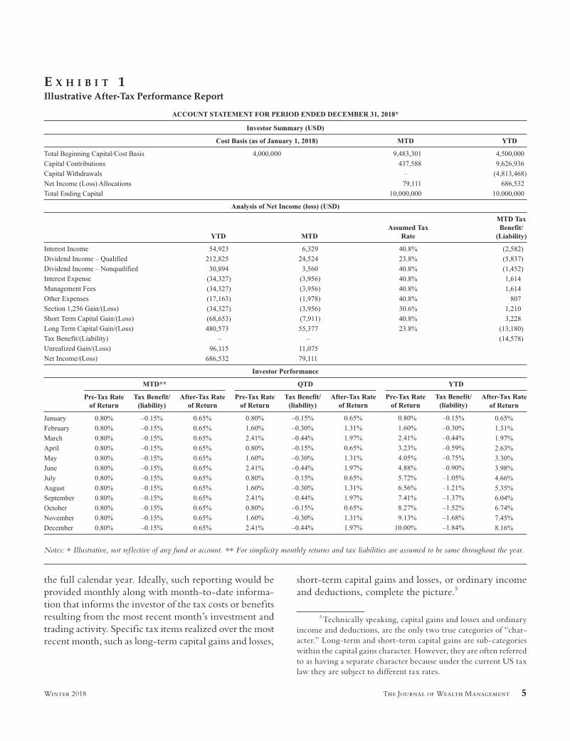
Exhibit 1 provides an illustrative example of our proposed monthly after-tax performance report for a hypothetical hedge fund for 2018 year-end.4 For sim-plicity of exposition, we assume that both pre-tax returns and taxable items (income, deductions, and realized gains and losses) as a percent of the fund’s NAV are constant over time. The top panel summarizes key pre-tax information for the current month and year: invested capital, contributions to and redemptions from the fund, and pre-tax appreciation of invested capital. Additionally, the top panel shows the beginning of the year cost basis of the investor.
The middle panel provides a more detailed break-down of contributions to net income for year-to-date and month-to-date including allocations of taxable gains, income, losses, and deductions. The year-to-date allocations in their respective tax character help investors manage their tax liabilities during the year by allowing them to estimate their taxable gains and income and potential taxable losses and deductions for
4 In all fairness, we are not the f irst to propose a specif ic after-tax performance report; see Stein, Langstraat, and Narasimhan (1999). In creating our report, we try to retain those features that can cost-efficiently be implemented by a third party fund administrator and remove those features that cannot (at least in the short term).
It is
ille
gal t
o m
ake
unau
thor
ized
cop
ies
of th
is a
rticl
e, fo
rwar
d to
an
unau
thor
ized
use
r, or
to p
ost e
lect
roni
cally
with
out P
ublis
her p
erm
issi
on.
The Journal of Wealth Management 5Winter 2018
the full calendar year. Ideally, such reporting would be provided monthly along with month-to-date informa-tion that informs the investor of the tax costs or benefits resulting from the most recent month’s investment and trading activity. Specific tax items realized over the most recent month, such as long-term capital gains and losses,
short-term capital gains and losses, or ordinary income and deductions, complete the picture.5
5 Technically speaking, capital gains and losses and ordinary income and deductions, are the only two true categories of “char-acter.” Long-term and short-term capital gains are sub-categories within the capital gains character. However, they are often referred to as having a separate character because under the current US tax law they are subject to different tax rates.
e x h i b i t 1Illustrative After-Tax Performance Report
Notes: * Illustrative, not ref lective of any fund or account. ** For simplicity monthly returns and tax liabilities are assumed to be same throughout the year.
It is
ille
gal t
o m
ake
unau
thor
ized
cop
ies
of th
is a
rticl
e, fo
rwar
d to
an
unau
thor
ized
use
r, or
to p
ost e
lect
roni
cally
with
out P
ublis
her p
erm
issi
on.
6 Multi-Period After-Tax Reporting: A PrActicAl Solution Winter 2018
Finally, the bottom panel of our illustrative report shows the multi-period pre-tax and after-tax returns for month-to-date, quarter-to-date, and year-to-date, as well as the components (pre-tax returns and tax costs and benefits) for computing them. The most recent month’s pre-tax return is computed by dividing “Net Income (Loss) Allocations” from the top panel, $79,111, by the invested capital in the beginning of the month (“Total Beginning Capital” plus beginning-of-month “Capital Contributions” minus beginning-of-month “Capital Withdrawals”), $9,483,301 plus $437,588, leading to 80 bps pre-tax monthly return. Similarly, the month-to-date tax benefit (liability) is computed as the “Tax Ben-efit/(Liability)” in the middle panel, -$14,578, divided by the invested capital—$9,483,301 plus $437,588—yielding a monthly tax cost of 15 bps. The after-tax return (65 bps) is then computed as the pre-tax return (80 bps) minus the tax cost (15 bps). Later, we detail the methodology used to compound single-period returns into multi-period returns. To more fully describe each section of the report and explain the rationale for the approach we chose, we next respond to eight key ques-tions about the report.
EIGHT NORMATIVE QUESTIONS ABOUT AFTER-TAX PERFORMANCE REPORTING
1. What Should the Reporting Frequency Be?
We suggest that after-tax reporting be produced with the same or similar frequency, typically monthly or quarterly, as currently provided for pre-tax reporting; otherwise taxable investors will be unable to perform meaningful organized tax management and planning for their investment portfolios, potentially harming long-term wealth accumulation.
In our stylized report, providing year-to-date allo-cations on a monthly basis, as shown in the middle panel of Exhibit 1 (“Analysis of Net Income (Loss) (USD)”), helps investors manage their tax liabilities throughout the year. For example, should the fund estimate having positive income or realized capital gains for the year, the investor can more effectively accelerate the liquida-tion of some investment losses into the current year in order to offset the anticipated income or realized gains. The character of income and gains—ordinary, long-term capital gains, or short-term capital gains—informs the investor about the specific type of losses that should
be realized in order to execute such tax management.6 In the opposite case, should the fund be expected to allocate losses, the investor might choose to accelerate liquidation of economically unattractive investments that are currently at a gain. Again, the reported char-acter of losses helps the investor decide which gains are best to realize.
By extension, the higher the frequency of reporting of gain and loss allocations, the easier it becomes for investors to optimize the after-tax performance of their overall investment portfolios. However, as frequent reporting imposes a burden on the fund manager and the fund administrator, we suggest a monthly frequency, which in our view strikes a reasonable balance between the investor’s benef it and the manager’s reporting burden.
2. What Information Should Be Included in the Report?
Tax character information is important for opti-mizing the investment portfolio’s tax efficiency. While a detailed description of tax character falls outside the scope of this article, the most common examples are realized long-term capital gains and losses, realized short-term capital gains and losses, mark-to-market capital gains and losses on qualified futures (otherwise known as § 1256 gains and losses), qualif ied income (e.g., qualified dividend income), ordinary income (e.g., investment interest or non-qualif ied dividends), and ordinary deductions (e.g., investment interest expense).7 These components are all displayed in the middle panel of Exhibit 1.
6 Note that losses are not necessarily liquidated when they become available. There is a tradeoff between the costs and ben-efits of loss-harvesting trades. The benefits result from realized losses offsetting taxable gains. These benefits should be weighed against transaction costs and the risk of deviating from the optimal investment policy due to the 30-day wash-sale period. When an investor has little or no taxable gains in the current year she might choose to avoid the costs and risks of loss-harvesting trades. When, however, she expects the tax benefit of offsetting taxable gains (and in particular short-term gains) to outweigh the transaction costs and economic risks of liquidating loss positions, acceleration of losses becomes attractive.
7 For calculating § 1256 qualif ied futures tax results, gains and losses should be appropriately split as 60% long-term and 40% short-term.
It is
ille
gal t
o m
ake
unau
thor
ized
cop
ies
of th
is a
rticl
e, fo
rwar
d to
an
unau
thor
ized
use
r, or
to p
ost e
lect
roni
cally
with
out P
ublis
her p
erm
issi
on.
The Journal of Wealth Management 7Winter 2018
In addition, fund investors may wish to understand the potential tax impact of redeeming from the fund, which might result in a tax on the difference between the value and the cost basis of their partnership interest.8 The beginning of year cost basis, reported in the top panel, allows the investor to estimate the tax cost of redemptions. To do this, the investor must first estimate the current cost basis by adjusting the beginning of the year cost basis upward for year-to-date contributions and allocations of income and capital gains and downward for year-to-date withdrawals and allocations of losses and deductions. All of this information is available in our stylized example shown in Exhibit 1: The top panel shows contributions and withdrawals, while income, gain, loss, and deduction allocations are reported in the middle panel.
We aggregate tax item allocation components over two time frames, year-to-date and month-to-date, shown in the middle panel of Exhibit 1. The former gives the investor an ability to plan and execute optimal levels of gain and/or loss realization at the level of the entire portfolio, while the latter allows the investor to drill down into the sources of the most recent month’s tax benefits and liabilities.
The information reported in the bottom panel of Exhibit 1 (“Investor Performance”) helps the investor monitor the fund’s after-tax performance on a monthly basis. We recommend that investors be provided with reports that display after-tax returns both incrementally and cumulatively as done in the bottom panel. For mon-itoring purposes, the report should show pre-tax returns and after-tax returns side by side along with the associ-ated tax benefits (or liabilities). Such reporting solves the “time-weighted return disinformation” problem (Lucas and Sanz 2016) mentioned earlier.
To calculate our single-period after-tax returns, we take the sum of the period’s pre-tax returns and the tax benefit or liability. However, this simple formula is not appropriate for multi-period after-tax performance reporting due to geometric compounding. The various components of after-tax returns—pre-tax return and tax cost or benefit—when compounded over multiple periods do not add up cleanly (geometric compounding
8 Capital gain allocations upon redemption, including both their magnitude and category (long-term or short-term), are subject to a complex set of rules and industry practices and is outside of the scope of the current discussion. The authors view the information provided in the current report as sufficient for a tax professional to be able to reasonably estimate the redemption tax liability.
introduces an unexplained residual). Fortunately, over the past several decades, an abundant literature has focused on addressing this multi-period performance attribution challenge.9 We draw upon this literature for our reporting purposes.
Specif ically, we chose to implement the Com-pounded Notional Portfolio method developed in Davies and Laker (2001), David (2006), and Berg (2014). This method allows us to separately cumulate multi-period pre-tax returns and multi-period tax ben-efits (or tax liabilities), and then by simply adding the two together, obtain multi-period after-tax returns. In Appendix A, we explain in more detail the computa-tions (and assumptions made) behind our multi-period return calculations.
3. How Should the Amounts of Income, Gains, Losses, and Deductions Be Determined?
Not to sidestep the question, but our suggestion for properly addressing this challenge is to find a good fund administrator. This is because determining the amounts and character of taxable items requires unique skills and competencies probably better handled by an administrator. First, correctly computing the tax items requires sophisticated tax software capable of not only tracking tax lots for each security in the portfolio but also making a variety of necessary tax adjustments including (but not limited to) correct characterization of income and expenses and identification of so-called “wash sales” and “tax straddles.”10 Such tax software is
9 Signif icant effort has been devoted to the issue of time-series linking of return contributions since the development of the Brinson, Hood, and Beebower (1986) single-period performance attribution model. Under this model the problem of multi-period attribution is similar to ours—arithmetically additive contributions need to be geometrically compounded over time. Popularity of the Brinson model led to the development of several methods to link arithmetic decomposition of returns over multiple periods. Leerink and van Breukelen (2015) divide these methods into two catego-ries: Smoothing Algorithms (e.g., Cariño 1999, Menchero 2000, and Frongello 2002) and Compounded Notional Portfolio (CNP) methods (e.g., Davies and Laker 2001, David 2006, and Berg 2014).
10 The unique tax treatment of different corporate actions is an additional challenge with which tax software must grapple. For example, Minck (1998) f inds that differences between after-tax returns computed with and without accounting for the unique tax treatment of corporate actions for the S&P 500 index from 1988 to 1997 was in a wide range of -29 to +34 bps per annum.
It is
ille
gal t
o m
ake
unau
thor
ized
cop
ies
of th
is a
rticl
e, fo
rwar
d to
an
unau
thor
ized
use
r, or
to p
ost e
lect
roni
cally
with
out P
ublis
her p
erm
issi
on.
8 Multi-Period After-Tax Reporting: A PrActicAl Solution Winter 2018
used and maintained by fund administrators that have the benefit of economies of scale across many clients and is likely impractical to be fully replicated in-house by a fund manager. This is especially true for actively man-aged hedge fund strategies that often utilize leverage and shorting and invest in a variety of instruments.
Second, the reporting of after-tax returns of com-mingled funds, such as securities limited partnerships, introduces an additional layer of complexity related to supporting partnership allocations of income, gains, losses, and deductions.11 Such allocations are best main-tained by a fund administrator.
Third, tax law and practice evolve over time. For asset managers whose primary duty is to keep abreast of markets and investment strategies, staying current with tax law developments falls outside their main focus and area of expertise and so might present a significant and unwelcome distraction. For administrators, on the other hand, it is one of their core services typically overseen by experienced tax professionals.
Finally, and perhaps most crucially, a fund admin-istrator serves as the fund’s official books and records that determine the f inal pre-tax income and taxable income, gain, and loss allocations at year-end. An inde-pendent administrator allows an objective approach and, when combined with the proper skills and systems, puts the administrator in a superior position to successfully accomplish accurate after-tax reporting.
For all these reasons, we partnered with a com-petent fund administrator in developing our detailed reporting consistent with Exhibit 1 that accurately cap-tures and updates relevant tax characters of income, gain, and loss throughout the year. The administrator maintains this reporting and provides it to investors on a monthly basis.
Before continuing, we should emphasize that having a good administrator does not relieve the fund manager from the duty of formulating the reporting framework. The administrator possesses the right tools and expertise for correctly identifying the items of tax allocations, but it is the manager’s responsibility to instruct the administrator on the content and frequency
11 See Sosner, Balzafiore, and Du (2018) for application of part-nership allocation rules to securities partnerships and Cunningham and Cunningham (2010) for a general introduction to partnership accounting.
of reporting and ensure that the fund investors receive such reporting in a timely manner.
4. Should Tax Losses Be Included in After-Tax Return Calculations?
In our view, after-tax reporting should account for the impact of both taxable gains and losses. This view is consistent with USIPC’s After-Tax Performance Stan-dards: USIPC (2011) § A.1.h requires that “each portfolio in the composite be given full credit for net realized losses, as it is assumed that these losses will be offset by gains at a later date or from other assets.” A given manager might have little visibility into the composition of realized gains and losses of other managers employed by a client. As a result, for the purposes of after-tax reporting, the man-ager should assume that all realized gains in her strategy result in current tax liabilities and all realized losses in her strategy provide current tax offsets against gains of the same character. This approach is ref lected in the last column (“MTD Tax Benefit/(Liability)”) in the middle panel of Exhibit 1.
Full consideration of losses merely ensures a sym-metric treatment of taxable gains and losses. While one might argue that to precisely measure the potential benefit of a fund’s tax losses it is imperative to under-stand the composition of taxable gains in the overall investment portfolio that these losses might offset, the same argument applies to taxable gains: It is impossible to accurately measure the tax burden of a fund’s tax-able gains without considering potential loss offsets from other investments.
We believe that accounting for the full benefit of tax losses paints a more accurate picture of a fund’s potential tax eff iciency. For example, a fund that in a given period allocates an equal amount of long-term capital gains and short-term capital losses, and thus has a zero net capital gain, has the potential to be more tax efficient in the context of an overall portfolio compared to a fund that allocated no capital gains or losses. This is because the short-term capital losses will offset highly taxed short-term capital gains (if such exist) before off-setting long-term capital gains.
The tax character of income, gain, loss, and deduction determines the applicable tax rates. In our report, we therefore multiply the amounts of income, gain, loss, and deduction by such applicable tax rates to estimate their contributions to the overall tax liability.
It is
ille
gal t
o m
ake
unau
thor
ized
cop
ies
of th
is a
rticl
e, fo
rwar
d to
an
unau
thor
ized
use
r, or
to p
ost e
lect
roni
cally
with
out P
ublis
her p
erm
issi
on.

The Journal of Wealth Management 9Winter 2018
In particular, accounting for permissible netting, losses and deductions in highly taxed characters reduce the total tax liability by a larger amount than those in low taxed characters.
5. What Tax Rates Should Be Used?
As the fund manager does not have visibility into every investor’s marginal tax rates, we must make cer-tain assumptions about the level of tax rates in order to report after-tax returns. USIPC (2011) § A.1.e provides the following guidance on tax rate assumptions: “after-tax returns must consistently utilize either the “anticipated tax rates” or the maximum federal (or federal/state/local/city) tax rate applicable to each client over time and within each composite.” For our reporting purposes, we employ the current (in our example in Exhibit 1), 2018 maximum federal tax rates applicable to investment income for a US individual increased by the 3.8% net investment income tax.
The detailed reporting of tax characters allows investors to manually adjust the rates—and thus tax ben-efits and liabilities—to fit their individual circumstances such as state and local tax rates or the Alternative Minimum Tax (AMT) tax rates.
6. How Should Investor Contributions and Redemptions Be Accounted For?
Methods of accounting for investors’ contributions and redemptions (hereafter referred to as “f lows”) can have a material impact on the fund’s return calcula-tions discussed earlier. USIPC (2011) provides three methods for calculating pre-liquidation after-tax fund returns (denoted below by RAT): Daily Valuation, Modi-fied Dietz, and Modified Bank Administration Institute (BAI) Linked Internal Rate of Return.
Of these three, we recommend relying as much as possible on the Daily Valuation Method defined as
= − −R
End Value Start Value Realized TaxesStart ValueAT
We use this method to report returns and tax liabilities in the bottom panel of Exhibit 1. Note that f lows do not explicitly appear in this formula because they are already included in the “Start Value.” Such inclusion of f lows in the start value, however, imposes particular reporting frequency requirements. Specifically, after-tax
return evaluation should be frequent enough such that no f lows occur in the middle of the evaluation period. In our stylized example in Exhibit 1, we report monthly and assume that f lows occur monthly on the first day of the month (as is true for most hedge funds).
The two other methods for computing pre-liquidation after-tax returns under USIPC (2011) are handy when f lows do occur in the middle of the evalua-tion period thus requiring approximations for the impact of these f lows on the growth of the fund’s assets. The USIPC prescribed calculations for pre-liquidation after-tax returns for these two methods are as follows.
Modified Dietz Method:
R
End Value Start Value Sum of Portfolio flows
Realized Taxes
Start Value Sum of Day Weighted Portfolio FlowsAT =
− −−
+
-
Modified BAI (Linked Internal Rate of Return) Method:
(1 ) ∑− = × +End Value Realized Taxes Flow Ri ATweighti
As mentioned, we prefer the Daily Valuation Method for computing after-tax returns, in particular in the presence of f lows. The following example illustrates why we advocate in favor of this particular method (and taxes are not needed to make the point).
Suppose that Fund A experiences a 10% pre-tax return in the first three months of the year, a -8% return in the last nine months of the year, no realized gains or losses (so no taxes), and no f lows. An investor contrib-uting $100 on January 1 would have achieved $110 on March 31 and $101.2 on December 31. The investor’s pre-tax return for the year is thus 1.2% (=$101.2/$100-1). Fund A would report this same return under all three USIPC return calculation methods.
Suppose now that Fund B has identical returns to Fund A, and similarly has no realized gains or losses. Unlike Fund A, however, Fund B doubles in size due to fund inf lows on the last day of the third month of the year. Investor 1 had $100 in the fund at the start of the year, which grows to $110 in the first three months (same as the investor in Fund A). Investor 2 then invests $110 on April 1, increasing the total fund AUM to $220. By the end of the year, due to the -8% return, the total assets of the fund had declined to $202.4.
It is
ille
gal t
o m
ake
unau
thor
ized
cop
ies
of th
is a
rticl
e, fo
rwar
d to
an
unau
thor
ized
use
r, or
to p
ost e
lect
roni
cally
with
out P
ublis
her p
erm
issi
on.
10 Multi-Period After-Tax Reporting: A PrActicAl Solution Winter 2018
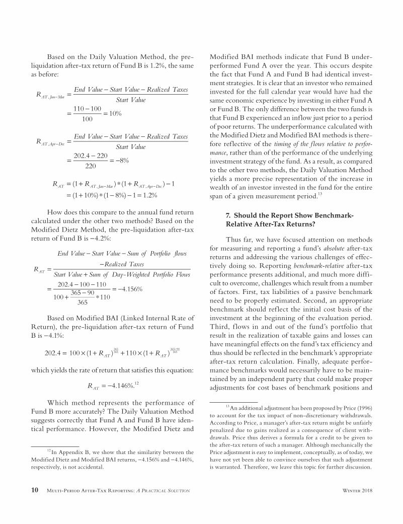
Based on the Daily Valuation Method, the pre-liquidation after-tax return of Fund B is 1.2%, the same as before:
110 100100
10%
,REnd Value Start Value Realized Taxes
Start ValueAT Jan Mar = − −
= − =
−
202.4 220220
8%
,REnd Value Start Value Realized Taxes
Start ValueAT Apr Dec = − −
= − = −
−
(1 ) (1 ) 1
(1 10%) (1 8%) 1 1.2%, ,R R RAT AT Jan Mar AT Apr Dec= + ∗ + −
= + ∗ − − =− −
How does this compare to the annual fund return calculated under the other two methods? Based on the Modified Dietz Method, the pre-liquidation after-tax return of Fund B is -4.2%:
R
End Value Start Value Sum of Portfolio flows
Realized Taxes
Start Value Sum of Day Weighted Portfolio FlowsAT =
− −−
+
= − −
+ − ∗= −
-
202.4 100 110
100365 90
365110
4.156%
Based on Modified BAI (Linked Internal Rate of Return), the pre-liquidation after-tax return of Fund B is -4.1%:
202.4 100 (1 ) 110 (1 )365365
365 90365= × + + × +
−
R RAT AT
which yields the rate of return that satisfies this equation:
4.146%.= −RAT12
Which method represents the performance of Fund B more accurately? The Daily Valuation Method suggests correctly that Fund A and Fund B have iden-tical performance. However, the Modified Dietz and
12 In Appendix B, we show that the similarity between the Modified Dietz and Modified BAI returns, -4.156% and -4.146%, respectively, is not accidental.
Modified BAI methods indicate that Fund B under-performed Fund A over the year. This occurs despite the fact that Fund A and Fund B had identical invest-ment strategies. It is clear that an investor who remained invested for the full calendar year would have had the same economic experience by investing in either Fund A or Fund B. The only difference between the two funds is that Fund B experienced an inf low just prior to a period of poor returns. The underperformance calculated with the Modified Dietz and Modified BAI methods is there-fore ref lective of the timing of the f lows relative to perfor-mance, rather than of the performance of the underlying investment strategy of the fund. As a result, as compared to the other two methods, the Daily Valuation Method yields a more precise representation of the increase in wealth of an investor invested in the fund for the entire span of a given measurement period.13
7. Should the Report Show Benchmark-Relative After-Tax Returns?
Thus far, we have focused attention on methods for measuring and reporting a fund’s absolute after-tax returns and addressing the various challenges of effec-tively doing so. Reporting benchmark-relative after-tax performance presents additional, and much more diffi-cult to overcome, challenges which result from a number of factors. First, tax liabilities of a passive benchmark need to be properly estimated. Second, an appropriate benchmark should ref lect the initial cost basis of the investment at the beginning of the evaluation period. Third, f lows in and out of the fund’s portfolio that result in the realization of taxable gains and losses can have meaningful effects on the fund’s tax efficiency and thus should be ref lected in the benchmark’s appropriate after-tax return calculation. Finally, adequate perfor-mance benchmarks would necessarily have to be main-tained by an independent party that could make proper adjustments for cost bases of benchmark positions and
13 An additional adjustment has been proposed by Price (1996) to account for the tax impact of non-discretionary withdrawals. According to Price, a manager’s after-tax return might be unfairly penalized due to gains realized as a consequence of client with-drawals. Price thus derives a formula for a credit to be given to the after-tax return of such a manager. Although mechanically the Price adjustment is easy to implement, conceptually, as of today, we have not yet been able to convince ourselves that such adjustment is warranted. Therefore, we leave this topic for further discussion.
It is
ille
gal t
o m
ake
unau
thor
ized
cop
ies
of th
is a
rticl
e, fo
rwar
d to
an
unau
thor
ized
use
r, or
to p
ost e
lect
roni
cally
with
out P
ublis
her p
erm
issi
on.
The Journal of Wealth Management 11Winter 2018
f lows in and out of a hypothetical benchmark portfolio. For all of these reasons, we suggest that the additional costs and complexity of reporting after-tax benchmark returns may not outweigh the benefits. We conclude that managers should use absolute rather than benchmark-relative after-tax reporting. Consistent with this recom-mendation, in the bottom panel of Exhibit 1, we show absolute—rather than benchmark-relative—returns and tax liabilities. We understand this recommendation may leave readers unsatisfied, and so we next turn to justi-fying our recommended approach.
Let’s consider each of these four issues in more detail. First, passive benchmarks are not necessarily free of capital gains taxes. For example, Sialm and Sosner (2018) estimate that for the period from 1985 to 2015, the average annual tax cost impact from realized gains for the Russell 1000 index using HIFO (high in, first out) accounting and 2015 tax rates (23.8% and 43.4% for long-term and short-term capital gains, respectively) was 25 bps.14 Such tax cost estimates require keeping track of tax lots of every positon in the benchmark, and are affected by the start date of the calculation (Stein 1998, Brunel 2000, and Price 2001) and the choice of method of accounting, e.g., HIFO or FIFO (Minck 1998, Dickson, Shoven, and Sialm 2000, Rogers 2006, and Israel and Moskowitz 2012).
Second, Minck (1998), Stein (1998), Stein et al. (1999), and Brunel (2000) emphasize the importance of considering the ratio of the initial cost basis to market value which changes with the age of the portfolio. This ratio matters because, over the same period, a new bench-mark portfolio is likely to have very different after-tax returns than a seasoned appreciated benchmark portfolio despite identical benchmark weights and pre-tax returns. These authors suggest various approaches to incorpo-rating an investor’s cost basis in after-tax benchmarking. For example, Minck (1998) and Stein (1998) simulate the after-tax performance of benchmark portfolios with dif-ferent start dates (“vintages”) and show that benchmark after-tax returns in a given year vary substantially by vintage. Older, more appreciated portfolios generally
14 These f indings are consistent with earlier studies of the impact of taxes on index portfolios. Minck (1998) using the HIFO (highest in, first out) method of accounting and 1987 tax rates (28% and 38.5% for long-term and short-term capital gains, respectively) estimates that between 1988 and 1997 the tax on realized gains of an S&P 500 index portfolio varied between -5 and 72 bps per annum, with an average of 28 bps.
underperform younger, less appreciated ones in after-tax terms. Brunel (2000) takes a different approach. Rather than categorizing portfolios by vintage, he proposes clas-sifying them according to the initial unrealized gains to market value ratios. These “baskets” of portfolios could then be used to create and report composites. Stein et al. (1999) propose a solution based on a theoretical approxi-mation which takes into account the evolution of the market value and the cost basis of the portfolio. In sum, there seems to be no industry consensus of whether and how to implement these various approaches to deal with these cost basis issues, imparting a serious constraint on effective after-tax benchmark performance reporting.
Third, after-tax returns of the benchmarks might be meaningfully affected by investor f lows. Dickson et al. (2000) show that outf lows can create negative tax externalities whereas inf lows may result in posi-tive tax externalities. In principle, some of this impact might be adjusted for using the methodology in Stein et al. (1999) and USIPC (2011), however, these adjust-ments are impractical to implement in the real world. Stein et al. (1999) propose treating an investment in the benchmark as one security in which key parameters are set to match the investor’s portfolio. These parameters would include (among other factors) dividend yield, cost basis, tax rates, gain realization rates, and, importantly, f lows. This way, a customized benchmark could be adapted to each investor by simply inputting assump-tions for each of the relevant parameters. USIPC (2011) describes a related approach, which involves the creation of “shadow portfolios” tailored to each investor. This approach begins by establishing the appropriate pre-tax index and calculating its after-tax returns. In order to compute the after-tax returns of the shadow portfolio, several assumptions need to be made to mimic the inves-tor’s portfolio. Similar to Stein et al. (1999), some such assumptions are the portfolio’s NAV, cost basis, tax rates, gain realization rates, and of course, f lows. Again, while the Stein et al. and USIPC approaches are compelling in theory, the myriad of assumptions and approxima-tions needed to successfully implement either of these approaches make them challenging in practice.
Finally, in order to avoid potential conf licts of interest, performance benchmarks should be computed by an independent party. The factors described above highlight the difficulties in reliably creating an after-tax benchmark. In light of these difficulties, until such after-tax benchmarks become available, we suggest managers
It is
ille
gal t
o m
ake
unau
thor
ized
cop
ies
of th
is a
rticl
e, fo
rwar
d to
an
unau
thor
ized
use
r, or
to p
ost e
lect
roni
cally
with
out P
ublis
her p
erm
issi
on.
12 Multi-Period After-Tax Reporting: A PrActicAl Solution Winter 2018
focus their efforts on reporting absolute, rather than benchmark-relative, after-tax returns.
To be clear, we are not suggesting that investors not use after-tax benchmarks in their evaluation of manager’s after-tax returns. One approach would be to compare manager’s after-tax returns to the after-tax returns of passively managed mutual funds or exchange traded funds (ETFs) applying the after-tax return calcu-lation methodology suggested by Morningstar (2013). In addition, for absolute return funds in which the pre-tax benchmark is defined by a short-term risk free interest rate such as 3-month Treasury bill rate, investors could use this rate reduced by ordinary tax rate as the bench-mark. A full investigation of this topic is beyond the scope of this article, and so we leave to future research how investors might utilize passively managed fund and ETF returns and interest rates in manager evaluation.
8. Should Managers Report Post-Liquidation Returns?
Adjusting after-tax returns for unrealized gains and losses is perhaps the most complex and ambiguous aspect of after-tax reporting. In order to turn appreciated positions into cash, a taxable investor must realize unre-alized gains and pay a capital gains tax often referred to as a “liquidation tax.” Unrealized gains thus create a gap between the observable market value and the true after-tax cash value of an investment, resulting in the following conundrum. On one hand, official books and records that can be reconciled among the fund man-ager, fund administrator, fund auditor and the inves-tor’s accountant do not ref lect theoretical adjustments for unrealized gains. However, in the absence of such an adjustment, all unrealized gains are effectively treated the same as would be tax-exempt income, thus poten-tially understating future tax liabilities. On the other hand, accounting for a tax burden associated with the full hypothetical recognition of unrealized gains, espe-cially for tax efficient funds where at least some unreal-ized gains may never be realized, may overstate the future tax burdens.15 Said differently, such full recognition of unrealized gains ignores the very real economic benefits
15 Taxes on unrealized capital gains are avoided when appre-ciated assets are donated to charity or receive a step-up of the cost basis at death.
of tax-conscious portfolio management that defers gain realizations in order to reduce tax costs.16
USIPC (2011) develops two methods, one for each end of the liquidation spectrum, for computing after-tax returns—one that does not account for any unrealized gains and another that fully recognizes all the unreal-ized gains in the current period. The first is the so-called “pre-liquidation” method, which accounts only for tax liabilities and benefits associated with gains and losses actually realized during the measurement period (as ref lected in the sample report in Exhibit 1). The second, defined by USIPC as the “mark-to-liquidation” calcu-lation methodology, assumes that all unrealized gains are realized, and therefore taxed, immediately. USIPC provides the following guidance: “The USIPC After-Tax Performance Standards require that after-tax returns be reported on a ‘pre-liquidation’ basis. The ‘pre-liquidation’ approach cap-tures the fact that taxes deferred to the future have a smaller present discounted value than taxes paid today.” It further says, “It is possible, however, that ‘mark-to-liquidation’ or ‘post-liquidation’ returns may also be presented to satisfy local regulations or to provide useful portfolio information for tax-able clients.”
All methods of post-liquidation return calculation involve some form of reducing the market value by the following quantity:
( )−ft V Vg m c
where f is a penalty coefficient, tg is the capital gains tax rate, and Vm and Vc are the current portfolio market value and cost basis, respectively. With the administrator systems discussed earlier, a frequent and up-to-date calculation of unrealized gains, Vm - Vc, is feasible. The problem, however, arises with the myriad of assumptions required to estimate an appropriate value of the penalty coefficient f.
The USIPC in their “mark-to-liquidation” method set f equal 1. However, the USIPC After-Tax Perfor-mance Standards only require reporting of after-tax returns on “pre-liquidation” basis and leave “mark-to-liquidation” to the discretion of the reporting manager. In Appendix C we outline the numerous inputs required
16 To be more precise, a tax-conscious manager will also keep track of, and prevent where possible, disallowance of realized losses due to wash sales and straddles and recognition of unrealized gains due to constructive sales.
It is
ille
gal t
o m
ake
unau
thor
ized
cop
ies
of th
is a
rticl
e, fo
rwar
d to
an
unau
thor
ized
use
r, or
to p
ost e
lect
roni
cally
with
out P
ublis
her p
erm
issi
on.
The Journal of Wealth Management 13Winter 2018
to estimate the value of the penalty coefficient f. These inputs include expected rate of future gain realization, expected investment horizon, expected pre-tax returns, probability of realizing gains upon liquidation, and probability of death. Unfortunately, these parameters come with such wide confidence intervals that nearly any value of the resulting coefficient f is possible.
In light of these diff iculties, it is not surprising that the USIPC After-Tax Performance Standards only require reporting of pre-liquidation returns. We also suggest that managers use the pre-liquidation method which relies on official books and records and does not require heroic assumptions on what will happen to the investor, to the strategy, to the level of tax rates, or to the market over a long and uncertain future period.17
CONCLUSION
Effective tax-aware investment management requires timely and informative after-tax performance reporting. However, most performance reporting models available today provide only pre-tax reporting, ignoring the after-tax aspects so relevant for taxable investors. This leaves taxable investors poorly serviced by the prevalent reporting paradigm whereby only pre-tax performance reports are made available during the year, and not until after the end of year do their accoun-tants typically prepare tax returns for the overall invest-ment portfolio. This makes it difficult, if not impossible, for investors to determine their true after-tax returns for the different components of their portfolio or even their portfolio as a whole. This approach not only muddles the relationship between contributions of individual managers to the taxable client’s after-tax wealth, but, perhaps even more problematic, hinders the execution of any organized tax planning throughout the year. In this article, we seek to resolve these issues by proposing an effective and workable after-tax performance report aimed at enhancing wealth preservation and accumula-tion for taxable investors.
Reporting and calculating after-tax returns is, however, quite challenging and requires a meaningful
17 We do encourage investors to estimate (at least qualitatively) their respective present values of liquidation tax costs. As our focus is on manager reporting, this topic is beyond the scope of this article. In this section and in Appendix C, however, we do provide investors some general guidance on issues related to estimating the present value of liquidation tax costs.
investment on the part of managers and fund administrators. We outline various aspects of this com-plexity that a manager committed to providing after-tax performance must navigate. Through an example, we illustrate and describe our proposed reporting approach, one that we have found to be an important and informa-tive tool for taxable clients when provided throughout the year by a fund administrator. With our approach, the tax character of incremental and cumulative gains and losses are reported, tax losses are considered to pro-vide an offset to taxable gains of the same character, returns and tax liabilities are properly adjusted for f lows using the USIPC Daily Valuation Method, and multi-period returns and tax results are linked using the Com-pounded Notional Portfolio methodology. Due to the sheer number of assumptions required to properly adjust for after-tax benchmarks or to compute post-liquidation returns, we chose to omit benchmark-relative and post-liquidation after-tax returns.
In sum, accurate and informative reporting of after-tax performance is an important issue that managers and investment advisors should not ignore. We do not claim to have a perfect solution; however, we offer one possible approach that, based on our experience, can be implemented in practice. We have written this article in the hope that other managers, advisors, and consultants will not only implement our suggested approach, but also review, comment, and improve upon our solution, leading to a better overall service for taxable investors.
a p p e N d i x a
MULTI-PERIOD RETURN CALCULATION
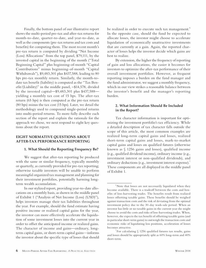
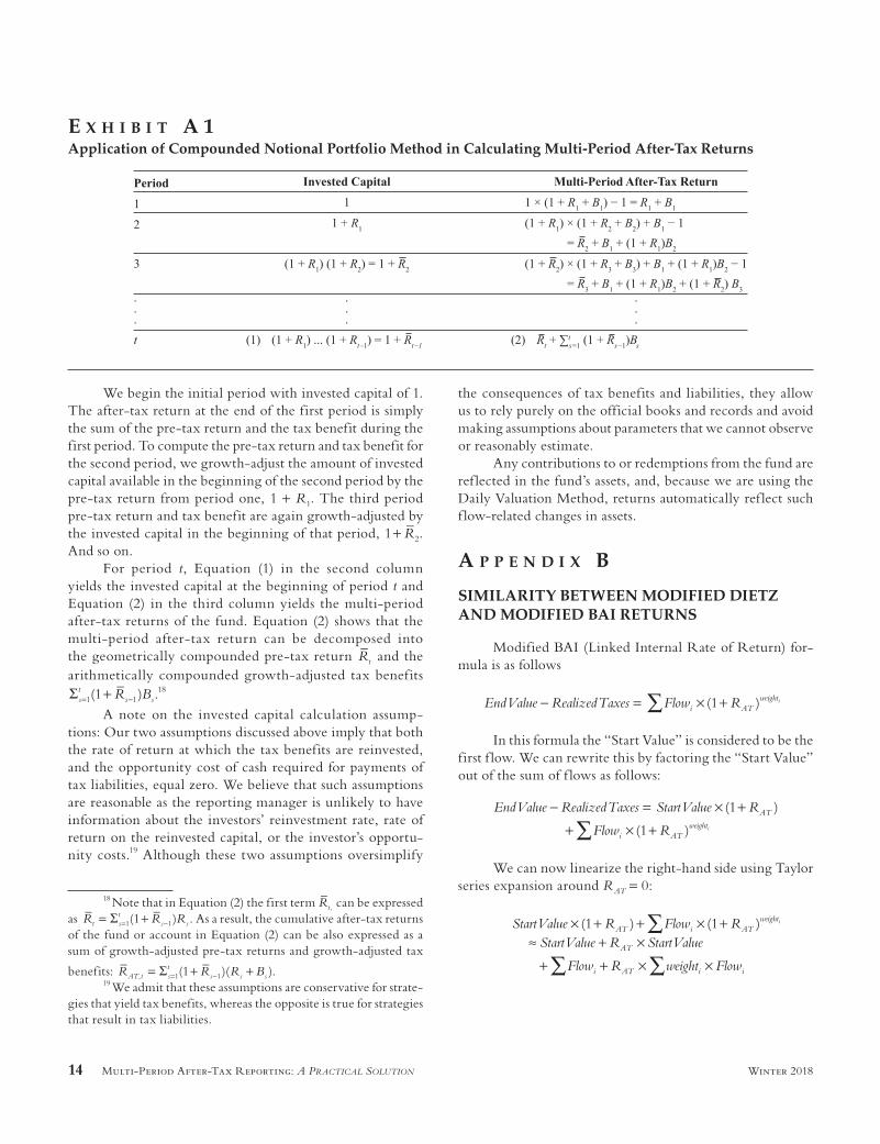
Exhibit A1 shows the details of our multi-period return calculations. For each period, we provide formulas for com-puting the amount of invested capital and the multi-period after-tax return. Rt represents the pre-tax return in period t, Bt is the tax benefit (if positive) or cost (if negative) in period t, both expressed as a percentage of invested capital, and Rt is the cumulative pre-tax return through period t computed as (1 )(1 ) (1 ) 11 2R R R Rt t= + + … + − , where 00 =R . In com-puting invested capital in the second column of Exhibit A1 we make two important assumptions: first, tax liabilities are paid from sources other than the assets of the fund; second, tax benefits are not reinvested back into the fund. As a result, the invested capital in each period grows by the pre-tax return of the previous period.
It is
ille
gal t
o m
ake
unau
thor
ized
cop
ies
of th
is a
rticl
e, fo
rwar
d to
an
unau
thor
ized
use
r, or
to p
ost e
lect
roni
cally
with
out P
ublis
her p
erm
issi
on.
14 Multi-Period After-Tax Reporting: A PrActicAl Solution Winter 2018
We begin the initial period with invested capital of 1. The after-tax return at the end of the first period is simply the sum of the pre-tax return and the tax benefit during the first period. To compute the pre-tax return and tax benefit for the second period, we growth-adjust the amount of invested capital available in the beginning of the second period by the pre-tax return from period one, 1 + R1. The third period pre-tax return and tax benefit are again growth-adjusted by the invested capital in the beginning of that period, 1 2+ R . And so on.
For period t, Equation (1) in the second column yields the invested capital at the beginning of period t and Equation (2) in the third column yields the multi-period after-tax returns of the fund. Equation (2) shows that the multi-period after-tax return can be decomposed into the geometrically compounded pre-tax return Rt and the arithmetically compounded growth-adjusted tax benefits
(1 )1 1Σ += −R Bst
s s.18
A note on the invested capital calculation assump-tions: Our two assumptions discussed above imply that both the rate of return at which the tax benefits are reinvested, and the opportunity cost of cash required for payments of tax liabilities, equal zero. We believe that such assumptions are reasonable as the reporting manager is unlikely to have information about the investors’ reinvestment rate, rate of return on the reinvested capital, or the investor’s opportu-nity costs.19 Although these two assumptions oversimplify
18 Note that in Equation (2) the first term ,Rt can be expressed as (1 )1 1= Σ += −R R Rt s
ts s . As a result, the cumulative after-tax returns
of the fund or account in Equation (2) can be also expressed as a sum of growth-adjusted pre-tax returns and growth-adjusted tax
benefits: (1 )( ), 1 1= Σ + += −R R R BAT t st
s s s .19 We admit that these assumptions are conservative for strate-
gies that yield tax benefits, whereas the opposite is true for strategies that result in tax liabilities.
the consequences of tax benefits and liabilities, they allow us to rely purely on the official books and records and avoid making assumptions about parameters that we cannot observe or reasonably estimate.
Any contributions to or redemptions from the fund are ref lected in the fund’s assets, and, because we are using the Daily Valuation Method, returns automatically ref lect such f low-related changes in assets.
A p p e n d i x B
SIMILARITY BETWEEN MODIFIED DIETZ AND MODIFIED BAI RETURNS
Modified BAI (Linked Internal Rate of Return) for-mula is as follows
(1 ) EndValue RealizedTaxes Flow Ri ATweighti∑− = × +
In this formula the “Start Value” is considered to be the first f low. We can rewrite this by factoring the “Start Value” out of the sum of f lows as follows:
(1 )
(1 )
EndValue RealizedTaxes StartValue R
Flow RAT
i ATweighti∑
− = × ++ × +
We can now linearize the right-hand side using Taylor series expansion around RAT = 0:
(1 ) (1 ) StartValue R Flow RStartValue R StartValue
Flow R weight Flow
AT i ATweight
AT
i AT i i
i∑
∑ ∑
× + + × +≈ + ×
+ + × ×
e x h i B i t A 1Application of Compounded Notional Portfolio Method in Calculating Multi-Period After-Tax Returns
It is
ille
gal t
o m
ake
unau
thor
ized
cop
ies
of th
is a
rticl
e, fo
rwar
d to
an
unau
thor
ized
use
r, or
to p
ost e
lect
roni
cally
with
out P
ublis
her p
erm
issi
on.
The Journal of Wealth Management 15Winter 2018
Note that
Flow Sumof PortfolioFlowsi∑ =
and
weight Flow Sumof Day Weighted PortfolioFlowsi i∑ × = -
such that the Modified BAI formula can be rewritten as
EndValue RealizedTaxes StartValueSumof PortfolioFlows R StartValueR Sumof Day Weighted PortfolioFlows
AT
AT
- ≈+ + ×+ ×
-
As a result, after rearranging this expression, it follows from, the Modified BAI method that
R
EndValue StartValue Sumof Portfolio flowsRealized Taxes
StartValue Sumof Day Weighted PortfolioFlowsAT ≈
− −−
+
-
The latter expression is the Modified Dietz formula. Thus the Modified BAI Method returns and Modified Dietz Method returns should be approximately equal.
a p p e N d i x C
EXTANT LITERATURE ON POST-LIQUIDATION PERFORMANCE
Stein (1998), Stein, Langstraat, and Narasimhan (1999), Poterba (1999), and Horan, Lawton, and Johnson (2008) propose alternative approaches to adjusting pre-liquidation after-tax performance for potential future tax liabilities asso-ciated with unrealized gains. Here we summarize their con-clusions and list the parameters required in their respective methodologies.
Stein et al. (1999), rather than relying on either pre-liquidation or post-liquidation values, use a “full cost equiva-lent” (FCE) approach derived in Stein (1998). FCE is the current cash value that, under the same investment strategy, will result in terminal wealth equal to that of the portfolio with embedded unrealized gains. (Cash value is used in this definition because cash has no unrealized gains.) Stein shows that mathematically, the FCE of a portfolio is its market value reduced by the following quantity:
( )−ft V Vg m c
where f is a penalty coefficient, tg is the capital gains tax rate and Vm and Vc are the current portfolio market value and
cost basis, respectively. Note that tg (Vm - Vc) thus represents a full liquidation tax liability. If the coefficient f equals 0, then FCE equals the pre-liquidation market value. A value of f equal to 1 implies full liquidation thus resulting in an FCE equal to a post-liquidation value. When the value of f is between 0 and 1, the liquidation tax value is adjusted downward because full liquidation does not happen immedi-ately. In Stein’s (1998) simulations, the coefficient f (and thus the effective liquidation tax liability) (i) increases with the expected rate of future gain realization, (ii) decreases with the expected investment time horizons, and (iii) decreases with expected pre-tax returns. In other words, lower returns, faster gain realization, and shorter investment horizons all lead to a higher expected present value of future tax costs of unrealized gains, thus reducing the FCE.
Similar to Stein (1998), Poterba (1999) recognizes that potential tax liabilities associated with unrealized gains should be valued based on their expected present value and not based on full and immediate liquidation. Poterba models this expected present value by using three probability param-eters: p, l, and q, where p represents the probability of selling the asset in a given year, l represents the probability that the sale does not generate a capital gain, and q represents the probability of dying in a given year (which captures the effect of a step-up in cost basis at death). Poterba shows that for a given level of annual after-tax nominal discount rate r, the expected value of tax liabilities associated with unrealized gain is equal to:
(1 )(1 )( )
− λ ++ + −
−p rr p q pq
t V Vg m c
As above, tg is the capital gains tax rate and Vm and Vc are the current portfolio market value and cost basis, respectively, and tg (Vm - Vc) represents a full liquidation tax liability. The multiplier in front of tg (Vm - Vc) effectively corresponds to Stein’s penalty coefficient f. The effects of different param-eters are also consistent with Stein. The probability of selling the asset, p, and the probability of realizing gain when selling the asset, 1 - l, are related to the rate of gain realization and, assuming positive after-tax nominal discount rate, r, both affect the multiplier positively. Increasing the probability of death, q, effectively increases the investment horizon: There is a correspondence between death and infinite investment horizon—both eliminate the liquidation tax, the former because of the step-up in cost basis, the latter because the liquidation never occurs. Similar to Stein, a longer invest-ment horizon and a higher pre-tax return (assuming that it is proportional to the after-tax nominal discount rate) reduce the penalty coefficient.
It is
ille
gal t
o m
ake
unau
thor
ized
cop
ies
of th
is a
rticl
e, fo
rwar
d to
an
unau
thor
ized
use
r, or
to p
ost e
lect
roni
cally
with
out P
ublis
her p
erm
issi
on.
16 Multi-Period After-Tax Reporting: A PrActicAl Solution Winter 2018
Horan et al. (2008) develop an after-tax value (ATV) measure which is the discounted present value of future post-liquidation value. Future post-liquidation value is derived analytically in Crain and Austin (1997) and Horan (2002). Similar to Stein (1998) and Poterba (1999), this future post-liquidation value depends on assumptions about the cur-rent cost basis, pre-tax returns, rates of gain realization, and investment horizon. An increase in the rate of gain realization has a negative effect on period-by-period after-tax returns, reduces the future effective liquidation tax rate (because unrealized gains are reduced through realization), and, under the assumption that ongoing tax rates are higher than the liq-uidation tax rate, reduces the overall ATV. This is consistent with both Stein and Poterba. Also, and as expected and in line with Stein and Poterba, an increase in the investment horizon and/or the pre-tax return reduces the effect of liquidation tax liability thus increasing the ATV.
ACKNOWLEDGMENTS
We are grateful for comments and suggestions by Phil Balzafiore, Jean Brunel, Michael Ferruzzi, Pete Hecht, Victoria Mukovozov, Ivan Paprikic, Ted Pyne, Clemens Sialm, and Roxana Steblea-Lora.
REFERENCES
Berg, C. V. 2014. “Exact Multi-Period Performance Attribu-tion Model.” The Journal of Performance Measurement (Summer): 47–63.
Brinson, G. P., L. R. Hood, and G. L. Beebower. 1986. “Determinants of Portfolio Performance.” Financial Analysts Journal ( July/August): 39–44.
Brunel, J. L. P. 2000. “An Approach to After-Tax Perfor-mance Benchmarking.” The Journal of Wealth Management, (Winter): 61–67.
Cariño, D. 1999. “Combining Attribution Effects over Time.” The Journal of Performance Measurement (Summer): 39–44.
Crain, T. L., and J. R. Austin. 1997. “An Analysis of the Trad-eoff between Tax-Deferred Earnings in IRAs and Preferential Capital Gains.” Financial Services Review 6 (4): 227–242.
Cunningham, L. E., and N. B. Cunningham. 2010. The Logic of Subchapter K. 4th Edition, West Academic Publishing.
David, M. R. 2006. “Sector-Level Attribution Effects with Compounded Notional Portfolios.” The Journal of Performance Measurement (Spring): 40–54.
Davies, O., and D. Laker. 2001. “Multiple-Period Perfor-mance Attribution Using the Brinson Model.” The Journal of Performance Measurement (Fall): 12–22.
Dickson, J. M., J. B. Shoven, and C. Sialm. 2000. “Tax Exter-nalities of Equity Mutual Funds.” National Tax Journal 53: 607–628.
Frongello, A. 2002. “Linking Single Period Attribution Results.” The Journal of Performance Measurement (Spring): 10–22.
Horan, S. M. 2002. “After-Tax Valuation of Tax-Sheltered Assets.” Financial Services Review 11: 253–275.
Horan, S. M ., and D. Adler. 2009. “Tax-Aware Investment Management in Practice.” The Journal of Wealth Management (Fall): 71–88.
Horan, S. M., P. N. Lawton, and R. R. Johnson. 2008. “After-Tax Performance Measurement.” The Journal of Wealth Management (Summer): 69–83.
Israel, R., and T. J. Moskowitz. 2012. “How Tax Efficient Are Equity Styles?” Chicago Booth Research paper.
Kahneman, D., and S. Frederick. 2002. “Representativeness Revisited: Attribute Substitution in Intuitive Judgment.” In T. Gilovich, D. Griff in, and D. Kahneman. Heuristics and Biases: The Psychology of Intuitive Judgment. Cambridge: Cam-bridge University Press, 49–81.
Leerink, B., and G. C. M. van Breukelen. 2015. “Multi-Period Performance Attribution: Framework for an Alloca-tion Effect Taking Active Weight Drift into Account.” The Journal of Performance Measurement (Summer): 34–51.
Lucas, S., and A. Sanz. 2016. “Pick Your Battles: The Inter-section of Investment Strategy, Tax, and Compounding Returns.” The Journal of Wealth Management (Fall): 9–16.
Menchero, J. 2000. “An Optimized Approach to Linking Attribution Effects over Time.” The Journal of Performance Measurement (Fall): 36–42.
Minck, J. L. 1998. “Tax-Adjusted Equity Benchmarks.” The Journal of Wealth Management (Summer): 41–50.
It is
ille
gal t
o m
ake
unau
thor
ized
cop
ies
of th
is a
rticl
e, fo
rwar
d to
an
unau
thor
ized
use
r, or
to p
ost e
lect
roni
cally
with
out P
ublis
her p
erm
issi
on.

The Journal of Wealth Management 17Winter 2018
Morningstar Research Report. 2013. “Morningstar After-Tax Return Methodology.” March 1.
Poterba, J. M. 1999. “Unrealized Capital Gains and the Mea-surement of After-Tax Portfolio Performance.” The Journal of Wealth Management (Spring): 23–34.
Price, L. N. 1996. “Calculation and Reporting of After-Tax Performance.” The Journal of Performance Measurement (Winter): 6–13.
——. 2001. “Taxable Benchmarks: The Complexity Increases.” AIMR Conference Proceedings (August): 54–64.
Rogers, D. S. 2005. “A Call to Arms! The Next Frontier for Taxable Accounts—After-Tax Return Performance Attribu-tion.” The Journal of Performance Measurement (Spring): 43–46.
——. 2006. Tax Aware Investment Management: The Essential Guide. Bloomberg Press (New York).
Sialm, C., and N. Sosner. 2018. “Taxes, Shorting, and Active Management.” Financial Analysts Journal 74 (1): 88–107.
Sosner, N., P. Balzafiore, and Z. Du. 2018. “Partnership Allo-cations and Their Effects on a Tax-Aware Funds’ Investors.” The Journal of Wealth Management (Summer): 8–17.
Stein, D. M. 1998. “Measuring and Evaluating Portfolio Performance after Taxes.” The Journal of Portfolio Management (Winter): 117–124.
Stein, D. M., B. Langstraat, and P. Narasimhan. 1999. “Reporting After-Tax Returns: A Pragmatic Approach.” The Journal of Wealth Management (Spring): 10–21.
United States Investment Performance Committee (USIPC). 2011. USIPC After-Tax Performance Standards. CFA Institute.
DisclosuresAQR Capital Management is a global investment management firm, which may or may not apply similar investment techniques or methods of analysis as described herein. The views expressed here are those of the authors and not necessarily those of AQR. AQR is not a tax advisor. This material is intended for informational purposes only and should not be construed as legal or tax advice, nor is it intended to replace the advice of a qualif ied attorney or tax advisor.
To order reprints of this article, please contact David Rowe at [email protected] or 646-891-2157.
It is
ille
gal t
o m
ake
unau
thor
ized
cop
ies
of th
is a
rticl
e, fo
rwar
d to
an
unau
thor
ized
use
r, or
to p
ost e
lect
roni
cally
with
out P
ublis
her p
erm
issi
on.