Electronic copy available at: http://ssrn.com/abstract=2089459

Working Paper No. 77 Chicago Booth Paper No. 12-20

How Tax Efficient are Equity Styles?

Ronen Israel AQR Capital Management

Tobias Moskowitz Booth School of Business, University of Chicago and NBER

Initiative on Global Markets The University of Chicago, Booth School of Business

“Providing thought leadership on international business, financial markets and public policy”

This paper also can be downloaded without charge from the Social Science Research Network Electronic Paper Collection:

http://ssrn.com/abstract=2089459

Electronic copy available at: http://ssrn.com/abstract=2089459

1

How Tax Efficient Are Equity Styles?

RONEN ISRAEL AND TOBIAS J. MOSKOWITZ ∗

Updated Version: July 2011

Abstract We examine the after-tax performance, tax exposure, and tax efficiency of size, value, growth, and momentum equity styles. On an after-tax basis, value and momentum outperform, and growth underperforms, the market. Decomposing the tax exposure of each style, we find that turnover is a misleading indicator of tax efficiency. Momentum, despite having more than five times the turnover of value, has the same tax rate as value, because momentum generates substantial short-term losses while value has high dividend income. In addition, tax optimization through capital gain and loss realization incurs less tracking error than avoiding dividend income. Hence, momentum, whose tax exposure is primarily driven by capital gains, while value and growth's taxes are more sensitive to dividends, is the only style that allows significant tax reduction without incurring significant style drift. The differential effects of taxes across equity styles are magnified within a broader asset allocation framework and in down markets.

∗Israel is a Principal at AQR Capital Management and Moskowitz is the Fama Family Professor at the Booth School of Business, University of Chicago and NBER. We thank Cliff Asness, Lauren Cohen, Jeff Dunn, Andrea Frazzini, Jacques Friedman, Marco Hanig, Brian Hurst, Bryan Johnson, Ryan Kim, Ralph Koijen, Oktay Kurbanov, Chris Malloy, Yao Hua Ooi, Lasse Pedersen, and Nathan Sosner for helpful comments. Sarah Jiang provided excellent research assistance. Moskowitz thanks the Center for Research in Security Prices for financial support. This research was funded in part by the Initiative on Global Markets at the University of Chicago Booth School of Business. Moskowitz has an ongoing consulting relationship with AQR Capital, which invests in, among other strategies, value and momentum.

Electronic copy available at: http://ssrn.com/abstract=2089459

2

Empirical asset pricing studies largely focus on the expected pre-tax real returns of asset classes and

equity styles. For a taxable investor, however, the after-tax returns of assets are the critical input for

investment decisions. We explore the after-tax performance, tax exposure and tax efficiency of

commonly used (both in academia and practice) equity style portfolios. Specifically, we focus on

equity styles based on size, value, growth and momentum, which dominate the cross-sectional return

landscape.

First, we examine whether the relative after-tax performance of these styles is different than

their pre-tax relative performance. Second, we decompose the capital gain, loss and income of each

style to identify the drivers of its tax exposure. Finally, we analyze how much after-tax returns can

be improved across styles through tax optimization and what the tradeoffs are between tax reduction

and tracking error.

Our study focuses mostly on long-only investable “passive” indices from July 1974 to June 2010

(e.g., Russell 1000 and Russell 2000 core market, value, and growth indices and AQR Capital

Management’s U.S. large and small capitalization momentum indices). In addition, we also examine

portfolios constructed from the Center for Research in Security Prices (CRSP) going back to 1927.

After-tax returns and effective tax rates are very consistent across these different portfolios within a

given equity style.

We find that the relative performance ranking of these styles is the same after-tax as it is pre-tax.

On an after-tax basis (but gross of transactions costs1), momentum delivers the highest average

returns among the styles, followed by value, the market, and then growth. We consider two different

tax code regimes: the current (2011) tax code and historical tax rates matched contemporaneously

through time with returns. The historical rates are on average more punitive because tax rates in the

early part of the 20th century are much higher than they are today. In addition, the mix of taxation

on capital gains versus income varies through time. Both of these features have different

consequences for different equity styles. We find that momentum outperforms growth by 217 bps

among large caps and by 402 bps per year among small caps using the 2011 tax rates. Using

historical tax rates, momentum outperforms growth by 119 bps among large caps and by 294 bps

among small stocks. Value also outperforms growth on an after-tax basis by 208 bps among large

caps and 307 bps among small caps under the 2011 tax code, and by 107 bps and 229 bps,

respectively, using historical rates. While the relative performance ranking of styles is preserved

after accounting for taxes, the effect of taxes mutes the return differences across styles. As stand- 1 For a treatment of real-world transactions in the context of value, growth and momentum strategies see Frazzini, Israel and Moskowitz (2011).

3

alone investments momentum and value face the highest effective tax rates, and hence, on an after-

tax basis the outperformance of value and momentum relative to growth and the market shrinks,

particularly under more punitive tax regimes.

Despite momentum having five to seven times the turnover of value, we find that value and

momentum face similar tax rates, but for very different reasons. Decomposing the tax exposure of

each equity style, momentum generates a lot of short-term losses (which offset many of its capital

gains) and more long-term gains. Value, on the other hand, has little net short-term capital gain

exposure, but generates significant dividend income, which is very tax inefficient. The nature of a

momentum strategy, which buys or holds onto recent winners and sells off recent losers, tends to

realize short-term losses and long-term gains. A value strategy is naturally exposed to high income

producing stocks with high dividend yields.

The effective tax rates of these styles also change significantly when viewed within the context

of a broader asset allocation strategy. The effective tax rate on momentum becomes significantly

smaller within a broader portfolio, whereas the effective tax rate for value remains largely the same.

This is because momentum's production of short-term losses provides an additional benefit by

offsetting other gains within a broader portfolio. On a stand-alone basis, capital losses that exceed

gains can only be carried forward according to the tax code, conferring future tax benefits to a stand-

alone momentum portfolio. But, within a broader portfolio, those excess losses may be used

immediately to offset other gains in the portfolio, providing additional current tax savings. Value, on

the other hand, which generates a sizeable fraction of its tax exposure from dividend income, has no

greater tax advantage within a portfolio as it does on a stand-alone basis, since income tax is treated

no differently within a broader portfolio. Within a broader asset allocation framework, therefore,

momentum's tax rate becomes much smaller than that of value, and similar to that of growth and the

market. The after-tax performance of momentum widens, outperforming value and growth among

large cap stocks by 1.20% and 3.09% per year, respectively, and outperforming small cap value and

growth by 2.29% and 4.95%, respectively. In contrast, the after-tax outperformance of value relative

to growth shrinks within a portfolio context, since value faces substantially higher dividend exposure

than growth and produces fewer short-term losses than growth.

Momentum is also particularly valuable to a taxable investor in down markets for similar

reasons. During times when significant short-term losses can be realized, an investment that

generates a lot of short-term losses can become more valuable in offsetting capital gains from other

less correlated investments within an asset allocation strategy. In down markets, the short-term

losses from momentum can actually increase the after-tax returns of the overall portfolio by about

4

4% per year. Among all the equity styles we consider, only momentum produces enough short-term

losses to improve returns from a pre-tax to a post-tax basis in down markets. All the other styles,

especially value, reduce after-tax returns even in extreme down markets because they contain heavy

dividend exposure which does not have this asymmetric feature. Conversely, momentum returns are

hurt more by taxes in an up market but not as much as they are helped by taxes in a down market.

Value, on the other hand, loses more than 1.20% per year in after-tax returns equally in up and down

markets due to its dividend exposure. Momentum, therefore, provides a taxable investor with an

implicit hedge in down markets, illustrated vividly during the recent economic crisis where

momentum lagged growth by 2.60% on a pre-tax basis, but outperformed growth by 5.90% after

taxes, and outperformed value by 8.23% per year on a pre-tax basis and by more than 17.14% after

taxes from July 2007 to March 2009.

We also examine an equal weighted (50-50) portfolio of value and momentum styles. We show

that the average of the after-tax value index return with the after-tax momentum index return is not

the same as the after-tax return of an equal-weighted combination of value and momentum. The

former, which we refer to as a simple combination, places $0.50 in value's after-tax return and $0.50

in momentum's after-tax return per dollar invested. The latter, which we refer to as an integrated

combination, places a $1 in a 50-50 value-momentum index and then computes the after-tax returns

on that 50-50 index. The difference in returns arises because the integrated combination takes into

account the interaction between the realized gains and losses generated by value and momentum

within the same portfolio, while the simple combination first computes after-tax returns for each style

separately (as stand-alone investments) and then takes an equal-weighted average, thus ignoring the

tax implications from the interactions between the two styles as well as the potential taxes incurred in

rebalancing back to 50-50 style weights. An integrated combination of value and momentum

outperforms a simple equal weighting of the value and momentum indices on an after-tax basis, and

both outperform the market.

Finally, we examine tax optimized or “tax managed” versions of our equity style portfolios to

see if conclusions drawn about the relative after-tax performance of these equity styles are altered

when tax optimization is considered. For example, if some styles lend themselves more easily to tax

management than others, then the relative after-tax performance of these styles could look quite

different. The indices and portfolios we (and the literature) examine are not designed to maximize

after-tax returns; hence it may be important to consider versions of the portfolios within a style that

try to minimize tax exposure.

5

We find that minimizing capital gains exposure (and ignoring dividends) improves after-tax

returns across all styles without incurring large tracking error or style drifts. Value and momentum

receive the largest after-tax improvements from capital gains optimization. However, we find that

dividend yield minimization (ignoring capital gain exposure) is detrimental to after-tax returns for all

equity styles except momentum. The stark difference in results between capital gains and dividend

minimization arises because an investor has more discretion on the timing of gain and loss realization

than on dividend income. Minimizing capital gains taxes entails shifting more realized gains to the

long-term and realizing more short-term losses, whereas the only way to reduce dividend income is

to sell the stock before the ex-date (which would trigger both a potential capital gain/loss realization

and the wash sale rule should the investor choose to buy the stock back after the ex-date), which

tends to have a much bigger effect on the portfolio. Tax optimization is, therefore, easier—in the

sense of not introducing tremendous tracking error—for strategies whose tax exposure comes mostly

from capital gains rather than dividends. In the case of value, which has high dividend exposure, a

reduction in dividends is equivalent to a reduction in value style. Value stocks are high dividend

paying stocks, so by selling or underweighting high dividend paying stocks the alpha of a value

strategy is depleted and the value style of the portfolio diminishes (e.g., its beta on a value

benchmark declines). Momentum, which has low dividend exposure, is less affected. A reduction in

dividend yield for momentum does not introduce style drifts since momentum stocks are low

dividend payers. Hence, tax optimization that minimizes capital gains and dividend exposure has the

biggest positive impact on momentum portfolios—improving after-tax returns without increasing

tracking error significantly.

We also find that an integrated combination of value and momentum outperforms value, a

simple combination of value and momentum and a combination of value and growth (e.g., the

market) when optimized for capital gains taxes and when optimized for both capital gains and

dividends. The interaction between value and momentum within a portfolio generates additional

returns net of taxes through tax management.

Our study is related to Bergstresser and Pontiff (2011) who examine the after-tax returns to

individuals, corporations, and broker-dealers on a set of benchmark portfolios that include the Fama-

French size, value, and momentum factors (SMB, HML, and UMD). Despite differences in

methodology, sample period, and examination of long-short as opposed to long-only portfolios, our

effective tax rate estimates are similar. The focus of our study is different, however, in that we

examine the tax efficiency of common equity styles, the components of each strategy that drive tax

exposure, and consider tax optimized versions of the equity styles to assess their relative tax

6

consequences and after-tax performance. Variation in the efficiency of tax minimization across styles

sheds new light on the tax efficiency and after-tax performance of these styles.

The paper proceeds as follows. Section I describes our data and portfolios and outlines our

methodology for constructing after-tax returns. Section II reports and compares the tax exposure and

after-tax returns of various equity styles taken from popular long only indices and the academic

literature. Section III examines how taxes can be minimized through tax optimization and trading

rules and compares the tax efficiency and after-tax returns across styles. Section IV concludes.

I. Data and Methodology

We detail our data sources and the equity style portfolios we examine. We also describe our

methodology for computing tax exposure and after-tax returns.

A. Data and equity style portfolios

We examine equity style portfolios among both large and small cap universes that cover the

market, value, growth and momentum styles. We focus on these equity styles because academic

research has shown these styles capture much of the cross-sectional variation in returns (Fama and

French (1996, 2008)), and are also, not coincidentally, the focus of attention in the investment

management industry, where investable indices are readily available.

We focus exclusively on U.S. equity indices and the U.S. tax code.2 For U.S. small and large

cap and value and growth equity styles we use for most of our analysis the S&P 500, Russell 1000,

Russell 1000 value and Russell 1000 growth indices for our large cap portfolios and use the Russell

2000, Russell 2000 value and Russell 2000 growth indices for our small cap portfolios. The Russell

1000 is a cap or value-weighted portfolio of the 1,000 largest stocks by market capitalization traded

on the NYSE, AMEX and NASDAQ as of June of each year. The Russell 1000 value Index is

comprised of the top 35-50% of stocks among the Russell 1000 that have the highest value

characteristics as determined by the highest book-to-price ratios and the lowest I/B/E/S forecast long-

term growth means. The Russell 1000 growth Index is comprised of the 35-50% of stocks with the

lowest book-to-price ratios and the highest I/B/E/S growth forecasts. Russell applies a non-linear

probability algorithm to the distribution of stocks based on these two variables that typically

identifies about the top 35% as value stocks, the bottom 35% as growth stocks and then weights the

middle 30% of stocks as both value and growth. The Russell 2000 index is a value-weighted 2 In a broader portfolio that includes international equities and other asset classes the net effect of taxes and the ability to minimize taxes can be very different, though we believe the implications addressed in this paper would be similar and could be extended in an international context.

7

portfolio of the next 2,000 largest stocks in the U.S., and the Russell 2000 value and growth indices

are defined as above among those 2,000 stocks. Russell excludes stocks trading below $1 per share,

pink sheet and bulletin board stocks, closed-end funds, limited partnerships, royalty trusts, foreign

stocks and ADRs. Reconstitution occurs annually in June of each year, where stocks deleted in

between reconstitution dates are not replaced, and spin-offs and IPOs are the only additions allowed

in between reconstitution dates.3 Dividends are reinvested on the ex-date.

Although momentum has been a part of academic studies for almost two decades, only recently

has an index exposed to momentum been available. AQR Capital Management in 2009 created a

large and small cap momentum index to capture this investment style. The momentum indices are

constructed as follows in a manner similar to the Russell methodology. Momentum is defined as the

past one year return for each stock, skipping the most recent month's return (cumulative monthly

return from t-12 to t-2). The AQR Large Cap momentum Index takes the 1,000 largest stocks in the

U.S. based on market capitalization and ranks each stock based on its past year return (from t-12 to t-

2), following the convention in the literature of skipping the most recent month's return to avoid

microstructure issues and high frequency and liquidity trades (see Jegadeesh and Titman (1993),

Asness (1994), Fama and French (1996, 2008), and Grinblatt and Moskowitz (2004)). The top third

of stocks based on momentum are then selected and value-weighted to form the momentum index.

The same process is repeated for the next largest 2,000 stocks to form the AQR Small Cap

momentum Index. The indices are reconstituted quarterly on the last day of each quarter. Stocks

trading below $1 per share, pink sheet and bulletin board stocks, closed-end funds, limited

partnerships, royalty trusts, foreign stocks and ADRs are excluded. Stocks deleted in between

reconstitution dates are not replaced, and spin-offs and IPOs are not added in between reconstitution

dates. Dividends are reinvested on the ex-date.

Our sample covers the period July 1974 to June 2010. The returns to the above indices are

available for most of the sample period: from July 1974 for the S&P 500, from July 1979 for the

Russell indices, and from January 1980 for the AQR indices. In cases where the index return series

begins later than July 1974, we extend the series back to July 1974 by replicating the index using the

CRSP universe of stocks and following, as closely as data availability allow, the official

methodologies outlined for each index above. We chose 1974 as our sample start date because

NASDAQ stocks first enter the CRSP universe in 1973, so 1974 is the earliest year we can start the

3 The Russell indices did not always reconstitute only in June. Prior to 1987, Russell reconstituted on a quarterly basis and then changed to semi-annual from 1987 to June 30, 1989. After that, Russell switched to an annual reconstitution process.

8

sample of returns and maintain stock universe consistency (since the momentum indices require a

year's worth of return history, the first return observation is in 1974). Another benefit of starting in

1974 is that the BARRA risk model is available, which we use for our tax optimizations in Section

III. As a check of our replication methodology, we compute the return correlation of each replicated

index versus its actual index over their overlapping periods in Table A1 of the Appendix. The return

correlations are consistently above 0.98 for the large cap indices and 0.92 to 0.99 for the small cap

indices.

We also examine an equal-weighted combination of value and momentum by placing 50%

weight in the value and momentum indices for both the large and small cap universes. The

motivation for looking at this combination is based on the observed benefits of combining value with

momentum—their positive risk premia and negative correlation to each other—documented by

Asness (1997) and Asness, Moskowitz, and Pedersen (2010).

In addition to examining investable indices, we also look at portfolios created and commonly

used in academic studies, notably those of Fama and French (1993, 1996 and 2008) obtainable from

Ken French's web site. A benefit of using these portfolios is that they provide returns going back to

1927. The drawback is they are not investable portfolios and only contain NYSE stocks prior to

1963. We examine the portfolios used by Bergstresser and Pontiff (2011), who also examine after-

tax returns and tax efficiency. These portfolios are the value-weighted CRSP index of all publicly

traded securities as a proxy for the market, the value-weighted portfolio of the top quintile of stocks

(using NYSE breakpoints) based on BE/ME ratio rankings as a proxy for value, the value-weighted

portfolio of the bottom quintile of stocks based on BE/ME rankings as a proxy for growth and the

value-weighted portfolio of the top quintile of stocks based on a ranking of cumulative past returns

from t-12 to t-2 as a proxy for momentum.

We focus exclusively on long-only portfolios and do not address the tax consequences of

shorting or the efficacy of after-tax returns for long-short style portfolios.

B. Tax Calculations

We detail below how we calculate the tax exposure and after-tax returns of the indices.

Tax rates. Tax rates are obtained from two sources: the Federal Individual Income Tax Rates

History 1913 - 2009 from the Tax Foundation in Washington, D.C. and historical capital gains rates

from the Department of the Treasury, Office of Tax Analysis (November 3, 2008). Table A2 in the

Appendix lists the year-by-year capital gains and dividend income tax rates for investors in the

99.99th and 95th percentiles of income in each year. We focus on the 99.99th income percentile to

9

calculate the maximum tax rate facing an investor, but present some results in the 95th income

percentile as well. Several years have a mid-year tax rate change, which we ignore in our analysis by

using the tax rates that existed at the beginning of the year. We also ignore differential capital gains

treatment for holding periods other than those less than one year and greater than one year. These

changes occur rarely and are typically small. Finally, dividend income tax rates reflect that of

qualified dividends, and we treat all dividend income from our portfolios accordingly, which is a

reasonable assumption based on the characteristics and reconstitution frequency of all the portfolios

we examine in the paper.

We consider two different tax code regimes. First, we apply the current 2011 tax code to our

portfolios historically. This analysis provides an evaluation of the average after-tax returns to the

portfolios under the current tax regime as a proxy for the expected after-tax return to each strategy

today. Second, we also employ historical tax rates as if the strategies had been run in real time by

adjusting the tax rates each year with changes in the tax code (according to Table A2) and aligning

them contemporaneously with returns through time.

Tax assumptions. In order to calculate the tax exposure of each portfolio and its after-tax

returns, we make the following assumptions. In addition to using the 99.99th income percentile tax

rates, we also adopt the HIFO system of identifying tax lots which entails taking the highest priced

stocks out first when applying taxes to the portfolio.4 Details of how we calculate the tax exposure

for each portfolio are provided in Section III.

We also compare the tax implications of each portfolio from two perspectives. First, we look at

each portfolio as a stand-alone investment, where losses are netted against any gains only within that

particular portfolio. Any losses exceeding the gains in a calendar year that cannot be used are then

carried forward according to the tax code. Second, we assume that all losses can be applied

immediately (no carry-forward of losses), which would be true in the context of a broader portfolio if

there are always gains coming from other investments against which to net those losses.5 The first

assumption imposes the maximum tax effect from capital gains, and the second assumption imposes

the minimum tax effect. Given that each of the portfolios we consider are typically part of a broader

asset allocation, it is important to consider these implications but also to recognize that the broader

4 Results are similar using a FIFO (first-in, first-out) or LIFO (last-in, first out) system for tax lots. An “optimal” methodology where one chooses which tax lots to relieve could potentially add even more value. 5 For most funds and accounts the netting of losses across investments is allowed, but for mutual funds, for instance, the IRS does not allow an investor to cross-net unused losses from one fund against gains from another.

10

portfolio may not necessarily always have adequate gains to net against. Thus, the true impact is

likely somewhere in between these two bounds.

II. After-Tax Returns and Tax Exposure of Equity Styles

We examine the after-tax returns of the equity portfolios, their effective tax rates and tax

exposures, and decompose their tax exposures into the component coming from capital gains and

dividend income separately.

A. Long Only Equity Style Indices

Table 1 reports the average annualized return before and after taxes on each equity style index

portfolio. All returns, pre- and post-tax, are reported before transactions costs.

The first column of Panel A of Table 1 reports the average annualized before-tax return on each

index. Among the large cap strategies, the Russell 1000 value outperforms the market indices,

Russell 1000 and S&P 500, by about 140 bps per year. The Russell 1000 growth index

underperforms the market indices by about 170 bps per year, and the AQR Large Cap momentum

index outperforms the market by almost 240 bps per year. These results are consistent with a long

academic literature that finds that momentum and value outperform the market and growth

underperforms the market on average, with momentum exhibiting the greatest outperformance.

Momentum outperforms value by more than one percent, and outperforms growth by just over four

percent per year. We also examine an integrated 50-50 equal weighted portfolio of value and

momentum by first creating a 50-50 value and momentum portfolio and then computing the after-tax

returns to that portfolio. As stated earlier, this integrated combination is different than a simple

averaging of the after-tax returns of value with those of momentum because of the interaction

between gains and losses from value and momentum within the same portfolio. We find that the

integrated combination outperforms the Russell 1000 (which is essentially a 50-50 integrated

combination between Russell 1000 value and Russell 1000 growth) by 1.5 percent per year. While

these comparisons simply take the difference in returns between portfolios without any risk-

adjustment, beta-adjusted returns or alphas yield nearly identical results.

Among the small cap strategies, we similarly find that value outperforms the market before

taxes, but by an even wider margin of 189 bps per year. Small cap growth underperforms the market

by about 2.38% per year, and small cap momentum outperforms the Russell 2000 by 3.87% per year.

These results, too, are consistent with those in the academic literature that find small value and small

momentum stocks deliver particularly large average excess returns, while small growth stocks

11

underperform significantly (Fama and French (1993), Hong, Lim, and Stein (2000), Grinblatt and

Moskowitz (2004), Israel and Moskowitz (2011)). Small cap momentum outperforms small cap

value by 1.99% and outperforms small cap growth by 6.25% per year. An integrated combination of

value and momentum among small caps outperforms the Russell 2000 index by 3.21% per year.

The next two columns of Panel A of Table 1 report the turnover (defined as the average of

dollars bought and sold divided by the imputed net asset value of each index) and dividend yield of

the style portfolios. Two key numbers stand out. First, the momentum indices generate substantially

more turnover than the other indices. This is partly due to quarterly rebalancing of the momentum

indices as opposed to annual rebalancing for the Russell indices, but it is also driven by the nature of

the momentum strategy, which uses market price data that updates more frequently than book-to-

market or earnings forecasts and hence generates more frequent changes in rankings among stocks.

The substantially higher turnover of a momentum style, however, does not necessarily mean it

exposes investors to higher capital gains taxes, since exposure to capital gains is a function of short

and long-term gains and losses, which are all embedded in turnover. A strategy with high turnover

coming from a lot of loss realizations does not expose an investor to capital gains, for instance.

Second, the value indices have much higher dividend yields than the other indices. High value

stocks tend to be high dividend paying stocks (relative to their market values) and hence expose

investors to high dividend income taxes.

A.1 Carry-forward Losses as a Stand-Alone Investment

The next four columns of Panel A of Table 1 report the annualized average after-tax returns of

the portfolios under the 2011 U.S. tax code and their effective tax rates, which are the differences

between the before- and after-tax returns divided by the pre-tax returns. We also report separately

the effective tax rates coming from capital gains and dividends. In Panel A of Table 1 we treat each

index as a stand-alone investment, netting out realized losses only against realized gains generated

from the portfolio itself and carrying forward any unused capital losses according to the tax code.

As Panel A of Table 1 shows, among the large cap styles, momentum has the highest effective

tax rate of 20.2%, followed by value with 13.7%, and then the market and growth indices with about

7%. On an after-tax basis, therefore, the outperformance of value and momentum styles diminishes,

though is still substantial. Value still outperforms growth by 208 bps, and momentum outperforms

growth by 217 bps and outperforms value by 8 bps after taxes. However, the tax exposures of the

value and momentum indices are very different. Value's tax exposure comes more evenly from

capital gains and dividend income, whereas momentum's tax exposure comes primarily from capital

12

gains. A 50-50 value-momentum portfolio outperforms the 50-50 value-growth (market) index by 83

bps after taxes.

A similar pattern is observed among the small cap portfolios. Here, however, the differences in

effective tax rates are smaller. Momentum has the highest effective tax rate of 22.7%, higher than

the 18.5% effective tax rate on the Russell 2000 value index and 14.3% tax rate on the Russell 2000

growth index. Once again, most of momentum's tax exposure comes from capital gains, whereas

small cap value has the largest dividend income exposure. On an after-tax basis, small value

outperforms small growth by 3.07%, and small momentum outperforms small growth by 4.02% and

outperforms small value by 0.95% per year. A 50-50 small cap value-momentum portfolio

outperforms the 50-50 value-growth (market) index by more than 1.91% per year after taxes.

The remaining columns of Table 1 report results repeating the analysis using the higher

historical tax rates. Since value and momentum have higher tax exposure, the higher tax rates will

mute their outperformance further. For large cap stocks under the more punitive tax codes, value’s

outperformance to growth on an after-tax basis gets cut in half to 107 bps, while momentum still

outperforms growth by 119 bps. An integrated 50-50 value-momentum combination still outperforms

value, a simple equal-weighted portfolio of value and momentum, and the market under the more

punitive tax codes among large cap stocks.

For small cap stocks, value outperforms growth by more than two percent per year, and

momentum outperforms growth by almost three percent per year under the higher historical tax rates.

An integrated 50-50 value-momentum combination continues to outperform value, a simple value-

momentum combination and the market index by over one percent per year under the more punitive

tax codes as well. Once again, the tax differences across the equity styles are much smaller among

the small cap portfolios than the large cap portfolios. Under the historical tax regime momentum still

generates most of its tax exposure through capital gains, but value produces disproportionately more

of its tax exposure from dividend income. These differences are key features that affect the ability to

minimize tax exposure across the equity styles, which we explore in Section III.

When we consider an investor at the 95th income level percentile rather than the 99.99th

percentile, we find an even higher after-tax outperformance for momentum and value. Table A3 in

the appendix shows that the lower tax rates at the 95th income percentile benefit momentum style

portfolios the most—adding an extra 10 to 20 bps on average to large cap momentum over large cap

value and an extra 30 bps versus large cap growth, as well as an extra 30 bps to small cap momentum

over small cap value and an extra 50 bps versus small cap growth. Consistent with the results

comparing the 2011 tax code to those using historical tax rates matched contemporaneously with

13

returns, less punitive tax structures on capital gains benefit momentum relative to the other equity

styles. While the 95th percentile tax rates may be more representative of the typical equity investor,

we use the 99.99th income percentile as a lower bound on the performance differences to be

conservative.

A.2 Using All Losses Immediately within a Broader Portfolio

Rather than treating each index as a stand-alone investment, where capital losses from each

index are netted only against capital gains from the portfolio and unused losses are carried forward,

Panel B of Table 1 repeats the analysis assuming all losses can be used immediately to offset other

gains in a broader portfolio.6 By assuming gains will always be present in the broader portfolio, this

analysis represents the minimum capital gains tax exposure for each style. The dividend tax

exposure of the style will be unaffected by this exercise. Under this assumption, styles in Panel A of

Table 1 that have significant unused losses being carried forward will now have much lower effective

tax rates since those losses will be applied immediately against other assumed gains.

Panel B of Table 1 reports the average annualized after-tax returns and effective tax rates under

the 2011 tax code and historical tax codes for each portfolio assuming all losses are used

immediately. Not surprisingly, the effective tax rates for every portfolio decline, and therefore after-

tax returns rise, when losses can be applied in a broader portfolio. The impact, however, varies

considerably across equity styles based on the amount of capital gains and losses each style

generates. For instance, the S&P 500, Russell 1000, and Russell 1000 value indices do not generate

a lot of capital losses and have more of their tax exposure from dividend income. Hence, the ability

to use losses in a broader portfolio is more limited for these styles. As a consequence, the after-tax

returns on these three indices all increase by less than 5 basis points (under the 2011 tax code). A

slightly larger improvement is found for the Russell 1000 growth index, where after tax returns go up

by 23 basis points per year when all loses can be used immediately. For momentum, however, there

is a substantial improvement. After-tax returns on large cap momentum rise by 116 basis points per

year (and its effective tax rate falls from 20.2% to 11.4%) when losses can be used immediately.

This result suggests that momentum is particularly valuable in the context of a broader portfolio

because it generates a lot of short-term capital losses that can be used to offset gains elsewhere in the

portfolio (or in the stand-alone case to offset future gains), while still on average generating a

positive average return. Viewed in this context, large cap momentum outperforms large cap value by

6 The tax code currently allows any losses to be used to offset any other investment capital gains, including real estate, derivatives, etc. But, these losses cannot be used against ordinary income including dividends and interest beyond the $3,000 per year allowance.

14

1.20% per year on an after-tax basis and outperforms large cap growth by 3.09% per year. In

addition, a 50-50 integrated value-momentum combination outperforms value, a simple value-

momentum combination, and the market index by 88, 28, and 140 bps, respectively, when all losses

can be used immediately. Relative to the market index, this difference is only 83 basis points when

losses are carried forward (Panel A), indicating that an integrated value-momentum combination also

generates significant realized losses that add an additional 57 basis points to returns.

Among small cap strategies, we see a similar picture. Negligible to modest improvements in

after-tax returns for the Russell 2000 market (10 bps), value (7 bps) and growth (48 bps) indices, but

substantial improvements for momentum (140 bps). Comparing Panel A to Panel B of Table 1, when

viewed as a stand-alone investment under the 2011 tax code, small cap momentum has the highest

effective tax rate (22.7%), but when viewed in the context of a broader portfolio, small cap

momentum has a lower effective tax rate (13.8%) than either the Russell 2000 (14.0%) or Russell

2000 value (18.0%) indices. As part of a broader portfolio, small cap momentum delivers an extra

2.29% per year in average after-tax returns over a small cap value portfolio and an additional 4.95%

per year over small cap growth on an after-tax basis. An integrated equal-weighted portfolio of value

and momentum also outperforms value, a simple combination of value and momentum and the

market index of small cap stocks by 1.49, 0.35, and 2.57 percent per year, respectively, after taxes.

Looking at the remaining columns of Panel B of Table 1, the higher tax rates from the historical

tax codes make the improvements from using capital losses even larger. Momentum benefits the

most from using realized losses and continues to outperform value and growth among large cap

stocks on an after-tax basis by more than 1.4% per year and outperforms value and growth among

small cap stocks by more than 2.1% per year. The benefits of applying realized losses within a

broader portfolio are substantial and are particularly relevant for a momentum strategy.

A.3 Decomposing Turnover

Our results highlight a common misconception: Turnover is a good indicator of capital gains tax

exposure. As the momentum strategies highlight, despite having five to seven times the turnover as

the other styles, the effective tax rate for momentum can be smaller than the other styles, because

momentum, which tilts towards recent past winners and away from recent past losers, realizes a lot of

short-term losses. Those short-term losses are valuable in offsetting gains not only from the

momentum portfolio itself, but potentially from other investments within a broader portfolio.

Table 2 decomposes the annual turnover of each equity style into short and long-term capital

gains and losses, reported as a percentage of the imputed net asset value of each index (i.e., per

dollar), where we assume each index started with a dollar investment at the beginning of the sample

15

period. For tax purposes, long-term gains are more efficient than short-term gains (because they are

taxed at a lower rate), and short-term losses are more efficient than long-term losses (because they

can be used to offset the higher taxed short-term gains). We report the percentage of total gains

coming from long-term realizations and percentage of total losses coming from short-term

realizations as indicators of the portfolio's tax efficiency.

Among the large cap portfolios, the market indices, S&P 500 and Russell 1000, are mainly

exposed to long-term gains, making them fairly tax efficient. However, neither of them generates

any short-term losses. As a stand-alone investment the market indices are therefore very tax

efficient, but in the context of a broader portfolio the lack of short-term losses makes them less tax

efficient. The Russell 1000 value index also has significant long-term gains, but in addition has non-

trivial short-term gains and generates very little short-term losses, which is why it is less tax efficient

than the market indices and contributes even less to the tax efficiency of a broader asset allocation

strategy. The growth index generates similar tax exposures as the value index with one key

exception. Growth generates more short-term losses than value. However, as the last column of

Table 2 indicates, about 3.3% (of NAV) of those losses on average have to be carried forward

because growth has lower returns overall, which makes it less tax efficient as a stand-alone strategy.

In the context of a broader portfolio, however, where those losses are assumed to be used

immediately, growth becomes more tax efficient, as evidenced by the larger increase in after-tax

returns highlighted in Panel B of Table 1. Finally, momentum generates a lot of long-term gains, a

lot of short-term gains, and substantial short-term losses. About 6.2% of those losses are carried

forward on average, so the tax efficiency of momentum is significantly improved in the context of a

broader portfolio where those additional short-term losses are assumed to be used immediately.

Among the small cap portfolios, we find a similar pattern. Value and growth produce about the

same amount of long-term gains, but much less short-term gains and losses than momentum. On a

stand-alone investment basis these tend to almost balance out as momentum only has a slightly

higher effective tax rate than value or growth. However, because a substantial fraction of those

short-term losses have to be carried forward on a stand-alone basis, in the context of a broader

portfolio where those losses are assumed to be used immediately, momentum's effective tax rate

declines significantly more than value's or growth's effective tax rate.

Turnover is a deceptive indicator of tax exposure. For example, much of the high turnover to a

momentum strategy has valuable or positive tax implications. As a simple metric to illustrate this

point, consider the ratio of effective capital gains tax rate-to-turnover for each equity style.

Momentum has the lowest ratio by far among the styles—its turnover is five to seven times higher

16

than the other styles but its tax rate is similar to the other styles. This suggests much of the turnover

to momentum strategies does not have negative tax consequences. Relative to its trading activity,

momentum is extremely tax efficient. Moreover, in the context of a broader portfolio, an added

dimension of momentum is its ability to generate additional short-term losses to offset gains from

other assets, making it even more tax efficient in an allocation setting.

Taxable investors, therefore, should not only seek out investments with attractive expected

return and correlation properties but also those with attractive tax implications for their overall

portfolio. The ability to generate short-term losses and long-term gains are characteristics of an

investment that taxable investors should value. In addition, taxable investors should tilt towards

lower dividend income exposure. These considerations are important when optimizing equity styles

for tax exposure, which we explore in Section III.

Figure 1 summarizes the results across the equity styles. Value portfolios provide positive pre-

tax alphas over the market index (among both large and small cap stocks), but expose investors to

substantial dividends and net short-term capital gains. Growth strategies have moderate dividend

yields and slightly negative short-term capital gains exposure, but deliver large negative pre-tax

alphas. Momentum, on the other hand, produces large positive pre-tax alphas, has reasonably low

dividend exposure and negative short-term capital gains among large cap stocks and small positive

short-term capital gains among small caps. Consequently, for a taxable investor the value premium

declines and the premium for momentum decreases slightly. Growth still continues to significantly

underperform the market, even on an after-tax basis.

B. Up and Down Markets

Since the gap between before and after-tax returns can be substantially different in rising versus

falling markets, we also examine the after-tax returns of the styles in up and down markets,

separately. Table 3 reports the after-tax performance of the equity styles in up and down markets,

defined as years in which the Russell 1000 index yields a positive and negative return, respectively.

By this definition, down market years are 1974 (second half), 1977, 1981, 1990, 2000, 2001, 2002,

2008, and 2010 (first half). Table 3 assumes that all losses can be used immediately in the context of

a broader portfolio and applies 2011 tax rates.

The first three columns of Table 3 report the pre- and post-tax average returns of the indices, as

well as their differences during up markets. On a pre-tax basis, momentum still produces the largest

average returns followed by growth, the market, and then value. The large cap momentum indices

outperform the value indices by 3.93% per year and outperform the growth indices by 3.62% in up

17

markets. The small cap momentum indices outperform the value indices by 4.76% per year and

outperform the growth indices by 4.77% in up markets. In a rising market, long-only equity

portfolios produce significant capital gains that expose an investor to taxes. So, naturally, the after-

tax returns of all the strategies decline. The largest declines occur for the momentum indices since

they generate the largest capital gains during these times. The value indices produce the next largest

declines both because of their capital gains and because of their substantial dividend income. The net

effect of taxes on momentum and value reduces momentum's outperformance by only about 1%,

leaving a premium relative to value of 2.47% in large cap and 3.69% per year in small cap on an

after-tax basis. Since the growth indices produce the smallest tax consequences in up markets, the

outperformance of momentum relative to growth on an after-tax basis diminishes as well, but still

remains at 1.15% for large cap stocks and 2.49% per year for small caps.

The next three columns of Table 3 repeat the analysis in down markets. Here, all the pre-tax

average returns are negative, with growth and then momentum delivering the most negative average

returns and value exhibiting the least negative returns. Before taxes, momentum lags value by 6.43%

per year, and outperforms growth by 4.95% among large caps in down markets.7 Among small caps,

momentum lags value by 3.95% per year and outperforms growth by 9.19%. However, when losses

can be used immediately, on an after-tax basis the returns to momentum actually rise, becoming less

negative on a post-tax basis. The returns to large cap momentum increase by 4.08% per year after

taxes in a down market, whereas large cap growth returns hardly change, and all the other styles

decrease, including large cap value which decreases by 1.20% per year after taxes. On an after-tax

basis, therefore, momentum only lags value by 1.15% in down markets and outperforms growth by

almost 8.95% in down markets among large caps. Among small caps, the story is the same.

Momentum improves on an after-tax basis by 3.26% while value declines by 1.81%. Hence, while on

a pre-tax basis small cap value outperforms small cap momentum by 3.95% in down markets, on a

post-tax basis small cap value lags small cap momentum by 1.11% in down markets—a 5.06%

turnaround attributable to the additional value of short-term loss realizations. Likewise, momentum's

superior performance over growth improves by another 1.65% on an after-tax basis in down markets.

These results highlight a unique aspect of momentum. In a down market, momentum implicitly

generates negative taxes, which can enhance returns in a broad portfolio that has gains elsewhere.

This occurs because a momentum strategy produces significant short-term loss realizations and in a

down market does not produce significant realized gains. If those losses can be used to offset gains 7 A great deal of the explanation for momentum underperforming value in down markets can be attributed to the difference in conditional betas of the two portfolios coming into down market environments (see Daniel (2011)).

18

in other parts of a broader asset allocation strategy (such as real estate, commodities, bonds or other

less correlated investments), they can net substantial tax savings that boost returns. Conversely, the

market portfolio and value strategies, in particular, produce positive taxes in both up and down

markets because most of their tax exposure comes from dividend income, which has the same tax

consequences in up and down markets. Put differently, dividends are much more stable than capital

gains and hence yield essentially the same tax consequences in good and bad market environments.

Hence, value strategies, which have significant dividend exposure, lose about 1.20% to 1.53% per

year after taxes in both up and down markets equally, whereas momentum strategies, whose tax

exposure is dominated by capital gains, lose about 3% in up markets from taxes but implicitly gain

almost 4% in down markets from taxes. A taxable investor, therefore, is provided an implicit hedge

in down markets from a momentum strategy.8

To further highlight this feature of momentum, the last three columns of Table 3 report the pre-

and post-tax returns of the indices over the recent economic crisis period from July 2007 to March

2009. On a pre-tax basis, momentum underperforms growth by 2.60% per year over this period.

However, on a post-tax basis assuming short-term losses can be applied, momentum actually

outperforms growth by slightly less than 6%. This is because momentum can potentially generate

more than 8% additional returns from its short term losses over this declining market, but growth

does not offer much tax benefit. Likewise, over this period momentum beat value by more than 8%

before taxes and by about 17% after taxes, due, again, to the additional benefit of tax losses

generated from momentum over this period.

The numbers presented in Table 3 represent the maximum tax benefit from being able to use all

capital losses immediately. This assumes an investor will always have sufficient gains which these

losses can be used to offset. That assumption is questionable in a down market. Hence, the

additional tax benefits calculated in Table 3 in down markets are an upper bound and are likely

smaller in practice. How much smaller depends on how sensitive the other parts of the portfolio are

to market downturns.

C. Equity Portfolios from 1927 to 2010

For robustness we also examine the returns to portfolios formed from CRSP data that go back to

1927, providing an additional 47 years of performance history. Specifically, we examine the

portfolios from Bergstresser and Pontiff (2011) created from CRSP that capture the market (CRSP

8 This is in addition to the ability of investors to harvest losses at the fund level by selling the fund and buying it back after the wash sale window passes.

19

value-weighted index), value (value-weighted portfolio of top 20% NYSE firms based on BE/ME

sorts), growth (value-weighted portfolio of bottom 20% NYSE firms based on BE/ME sorts) and

momentum (value-weighted portfolio of top 20% NYSE firms based on past one year returns,

excluding the most recent month).

Panel A of Table 4 reports the average annualized before and after-tax returns and effective tax

rates of the portfolios from Bergstresser and Pontiff (2011) who cover the period June 1927 to June

2007. Bergstresser and Pontiff (2011) report results under two different tax regimes: 2000 tax rates

and historical tax rates going back to 1927 matched contemporaneously with returns. Losses are

assumed to be available for immediate use in the context of a broader portfolio.

The portfolios used by Bergstresser and Pontiff (2011) are value-weighted and hence are

probably best compared with the large cap indices we examine. As Panel A of Table 4 shows, the

annualized after-tax returns and effective tax rates under the 2000 tax code are very consistent with

those for our indices covering the shorter 36-year period. Momentum and value generate the largest

tax burdens, but the effective tax rates across the market, value, growth and momentum strategies are

similar. Using the historical tax rates, the effective tax rates on the Bergstresser and Pontiff (2011)

portfolios are generally higher than what we find for our indices because tax rates in the early part of

the 20th century are much higher than in recent times. However, the relative ranking of portfolios

based on tax burden and after-tax performance remains consistent with our earlier results.

Momentum outperforms value by 58 (29) basis points per year on an after-tax basis and outperforms

growth by 315 (204) bps per year after taxes using year 2000 (historical) tax rates. A 50-50 value-

momentum combination outperforms the market portfolio by 227 (131) bps per year after taxes using

2000 (historical) tax rates. These magnitudes are also consistent with those from our earlier analysis.

Panel B of Table 4 updates the Bergstresser and Pontiff (2011) results through June 2010. Since

the period from July 2007 to March 2009 is an extreme one, it is useful to see how the numbers are

affected by this extreme episode. As Panel B shows, updating the returns through 2010 hurts

momentum and value relative to growth, but only by a small margin. When adding the most recent

data, the after-tax returns of momentum, value, and growth strategies (based on year 2000 tax rates)

drop by 70, 90, and 53 basis points, respectively. Although the 83-year average returns are affected

by the recent economic crisis, the relative performance numbers stay consistent. For example,

momentum's after-tax outperformance of growth drops by only 17 basis points, and still remains at

almost 3% per year. Value, which suffers even more than momentum over this extreme period, lags

momentum by an additional 20 basis points when the recent period is included, resulting in a total of

78 basis points difference between value and momentum on an after-tax basis over the entire period.

20

The after-tax returns and effective tax rates for these equity styles over the longer 83-year period are

very similar to those from our investable indices over the shorter sample period, including the most

recent period of extreme returns.

III. Tax Optimization and Tax Efficiency

To more fully address the tax efficiency of equity styles, we consider tax-optimized versions of

the style portfolios. The portfolios analyzed so far are not designed to optimize or pay attention to

taxes in any way and hence may be quite tax inefficient. In order to fully answer how tax efficient

various investment styles are it seems crucial to evaluate how taxes can be minimized within a style.

Does growth, value or momentum lend itself more easily to tax optimization? How tax efficient can

each of these styles become if portfolios are designed to minimize taxes?

In this section, we attempt to maximize the after tax return of each strategy. We design “tax

managed” versions of our indices that optimize the capital gains and dividend exposure of each style

to maximize after-tax returns. Comparing the after-tax returns of the original/tax unaware versions to

those of the tax managed versions also provides us with a sense of how large the improvements in tax

efficiency are, which we then compare across equity styles.

A. Minimizing Capital Gains Exposure

We start by attempting to minimize the tax consequences from capital gains for each style,

ignoring dividend income. We consider altering the portfolios' dividend exposures in the next

subsection. The objective is to minimize capital gains taxes, subject to maintaining the style of the

original portfolio. Thus, we place a tight constraint on the amount of tracking error or style drift we

allow the optimized portfolio to have. We want to optimize for capital gains tax exposure but not at

the expense of producing a portfolio that is too dissimilar from the equity style itself.9 The

optimization assumes that expected returns are equal across all stocks, so minimizing capital gains

taxes is equivalent to maximizing expected after-tax returns. This assumption simplifies the

optimization such that changing the weight on a security is only a tradeoff between the marginal

benefit of lowering the capital gains tax versus the marginal cost of introducing more tracking error

to the original portfolio. Allowing securities to offer different expected returns would introduce a

third dimension the optimization could pursue, but would also require a model of expected returns.

9 For example, we could buy and hold a portfolio and never trade for the entire 36 year period, thus minimizing capital gains, but this portfolio would not look anything like its intended style.

21

While this additional tradeoff could be interesting, it is beyond the scope of this paper. Instead, we

assume the original portfolios are optimal in the absence of taxes, with respect to their equity styles.

In order to specify the tax optimization problem, we first define the capital gains tax liability for

an individual stock trade, then extend this definition to the basket of stock trades, and finally discuss

how we measure tracking error.

Let St be the number of shares of a given stock held in the portfolio at time t and ΔSt = St - St-1 be

the change in shares from time t-1 to t. For the purposes of calculating the tax liability, we are

concerned with trades where ΔSt < 0; in other words, sales of shares. Once a sale occurs, it triggers

potential tax liability, depending on whether there is a gain or loss realization which is determined by

comparing the dollar value of the sale at time t to the original cost basis of the position in the stock.

The cost basis is determined by the trade prices and trade quantities on the acquisition dates of the

stock. For the purposes of computing taxes, these past acquisitions of shares are recorded in “tax

lots” which are further defined below. The sale of a particular stock's shares today can involve

multiple tax lots, where any or all of the past purchases of the stock's shares can be used in

determining the cost basis. Therefore, to determine the cost basis for a given sale, a system of

identifying tax lots must be adopted. The FIFO (first-in, first-out) system orders tax lots from oldest

to most recent purchases and uses the earliest purchases first to determine tax lots. The LIFO (last-in,

first-out) system uses the most recent purchases first to determine tax lots. We use the HIFO

(highest-in, first-out) system of identifying tax lots which uses the highest purchase price of past

stock buys to order tax lots and applies the highest priced tax lots first.

Formally, we define each tax lot for a single stock at a date t, which is a day on which shares

were acquired. Tax lots are represented in terms of the number of days since acquisition, the average

trade price on the day the shares were purchased and the quantity of shares purchased for each

acquisition date. Each tax lot has a unique trading day, where all shares purchased on a given day are

aggregated at the average trade price at which those shares were acquired on that day (e.g., multiple

trades on a given day are aggregated at the daily level)10. We define the matrix of tax lots L

pertaining to the sale of stock i on date t (e.g., ΔSi,t < 0) as,

10 It is standard industry practice to aggregate trades done on a particular day into one trade ticket per name and per side (if there are both buys and sells in the name on the same day) at the average trade price for that day’s trades. The methodology described in this section could be applied to multiple trade tickets in a name per day without loss of generality. Given the standard tax lot identification methods described in this section, any differences in tax lot identification between whether trades are aggregated per day or not would be limited and economically small.

22

( 3) ( 1)( 1) ( 1); ;

where,# days since shares were acquiredaverage trade price of shares on day of acquisition, quantity of shares traded at time of acquisition, number of

n nn n

t d

t d

P S d

dP PS Sn

× ×× ×

−

−

=

====

L

tax lots

Since it is often the case that the sum of shares from the tax lots exceeds the number of shares sold at

time t (the exception being a liquidation of all shares held in the stock which would equal the sum of

all tax lots), an investor must choose a subset of tax lots to use for the cost basis. The U.S. tax code

allows an investor to choose an approach for tax lot determination that must be applied consistently

throughout the portfolio. For example, a rules-based approach that orders tax lots along a dimension.

One popular method is FIFO (first-in, first-out) as described above, which sorts the matrix of tax lots

L by its third column, d, in descending order. LIFO (last-in, first-out) sorts L by d in ascending

order. We use the HIFO (highest price, first-out) system which sorts L by its first column, P, in

descending order from highest to lowest price. In principle, one could sort tax lots by quantity of

shares (the second column of L) to minimize or maximize the number of tax lots used, or sort by

some function of P, S, and d that minimizes taxes (often referred to as “optimal” tax lot

determination). We use the HIFO system rather than an optimal system, which in theory understates

the tax benefits.

Under the HIFO system, we reorder the matrix L by column one (price) from highest to lowest

such that: (1,1) (2,1) (3,1) ( ,1)n≥ ≥ ≥L L L L . The number of whole tax lots, K, used to compute

the cost basis for the stock sale is determined by:

1

arg max s.t. ( , 2) , where K

tk

K k S K n=

= ≤ −∆ ≤∑L (1)

The tax exposure for this single stock trade for stock i is then given by the following two equations,

separated into short and long-term tax exposures, where K = KST+ KLT, representing the number of

short and long-term tax lots separately.

( ) ( )1 1

Short-term tax exposure:

( , 2) ( ,1) ( , 2) ( 1,1) ( ,3) 365ST STK K

i t t t STl l

STX l P l S l P K l= =

= − + −∆ − − + ∀ ≤

∑ ∑L L L L L

(2)

23

( ) ( )1 1

Long-term tax exposure:

( , 2) ( ,1) ( , 2) ( 1,1) ( ,3) 365LT LTK K

i t t t LTl l

LTX l P l S l P K l= =

= − + −∆ − − + ∀ >

∑ ∑L L L L L

(3)

The first expression of the short and long-term tax exposures in equations (2) and (3) represents the K

tax lots that are fully utilized, and the second part of each equation captures any remaining shares

from the stock sale that only partially fill the last tax lot. Thus, the tax exposure for this single stock

trade is the sum across all relieved tax lots of the value received upon sale minus the cost basis for

each lot, categorized as short-term if there is a sale of shares within one year (365 days) of the

purchase date, and long-term if there is a sale of shares more than a year from the purchase date.11

The short and long-term tax exposures can each be positive or negative. A positive number

represents net realized gains, and a negative number represents net realized losses that we assume

can either be used immediately to offset other gains or are carried forward according to the tax code

for future use (without loss of generality for the optimization we assume the discount rate for carried

forward losses is zero).

Summing up the tax exposures across all N stock sales in the portfolio at time t, we get the

following for the tax liability of the entire portfolio:

( )

( )1 1 1 1 1

1 1 1 1 1

1 1

if 0 and

if 0 and

otherwise

N N N N NLT

i i t i i i ii i i i i

N N N N NST

portfolio i i t i i i ii i i i i

N NST LT

i t i ti i

STX LTX STX LTX STX LTX

TL STX LTX LTX STX LTX STX

STX LTX

τ

τ

τ τ

= = = = =

= = = = =

= =

+ < < ≤

= + < < ≤

+

∑ ∑ ∑ ∑ ∑

∑ ∑ ∑ ∑ ∑

∑ ∑

(4)

The U.S. tax code allows for short-term losses to offset short-term gains and long-term losses to

offset long-term gains such that only the net gains and losses of the portfolio are taxed. The tax code

requires that short-term losses must be used first to offset short-term gains and then any remaining

short-term losses can be applied to offset any remaining long-term gains. Likewise, long-term losses

must first be used to offset long-term gains, and then any remaining long-term losses can be applied

to any remaining short-term gains. In the event total net losses exceed total net gains the losses can

11 The U.S. tax code uses 365 days to define a year except for leap years, when an additional day is added. Equations (2) and (3) indicate year definitions of 365 days for simplicity, but we use 366 days in leap years for our calculations.

24

be carried forward for future use, but those losses must retain their character such that carried

forward short-term losses must first be applied to future short-term gains and carried forward long-

term losses must first be applied to future long-term gains. Thus, short-term losses are more valuable

from a tax perspective than long-term losses since long-term losses have to be applied first, both

contemporaneously and in the future, to lower taxed long-term gains. Equation (4) captures all of the

possible scenarios with respect to netting of short and long-term gains and losses within a portfolio.

The first part of equation (4) handles the scenario where there are net short-term losses and net long-

term gains, where the amount of net short-term losses does not exceed the net long-term gains. The

remaining net gains in this scenario are therefore taxed at the long-term rate. The second part of

equation (4) deals with the case where there are net long-term losses and net short-term gains where

the amount of net long-term losses does not exceed the net short-term gains. These remaining gains

are taxed at the short-term rate. The last part of equation (4) captures all other scenarios: short and

long-term gains taxed at their respective rates, short and long-term losses, which provide negative tax

benefits that are either carried forward or applied to gains within a broader portfolio, at their

respective tax rates, and the netting of short-term losses against long-term gains when those losses

exceed the gains as well as the netting of long-term losses against short-term gains when losses

exceed gains, where the carried forward losses retain their short and long-term status for future use.

We minimize the tax liability of the portfolio subject to a tracking error constraint defined

relative to the original index using a risk model to measure the contribution each security makes to

the overall tracking error of the portfolio. We use two risk models for robustness: the USE3S

BARRA risk model (US Short-Term model) and the Fama and French three factor model augmented

with a fourth momentum factor. We describe below the details of these models and how we use

them to measure tracking error.12

Using these risk models, the tax optimization problem is,

12 We also ran optimizations that simply minimized the Cartesian or sum of squared distances between the new portfolio weights and the original weights, which alleviates the need for specifying a risk model. However, this method of measuring tracking error ignores the correlation structure of returns and assumes homoskedasticity across stocks. It is equivalent to assuming the identity matrix for the covariance matrix among securities. Nevertheless, we obtain qualitatively similar results using this method.

25

*

min

. .t

portfolio

t t

t tt

t t

t B

TL

s t

c′ ′Ω + Σ ≤

=′

w

* * *

*

w w w wS PwS P

w = w - w

(5)

where tw is the vector of chosen portfolio weights after all trades at time t, defined as the vector of

shares owned in each stock times their price at time t (where denotes the Hadamard or entrywise

element-by-element matrix product) divided by the total dollar value of the portfolio, t t′S P , and Bw

is the vector of portfolio weights of the index or benchmark portfolio we want to rebalance with

respect to, which, in our case, is the optimal portfolio in the absence of taxes. Thus, w* would

represent the change in weights between the new portfolio at time t and the benchmark portfolio. Ω is

the covariance matrix of stocks from the risk model, Σ is the covariance matrix of residuals from the

risk model, and c is some pre-specified risk or tracking error constraint. The covariance matrix and

residual risk estimates come from the one-month lagged USE3S BARRA risk model (US Short-Term

model), which is a factor based risk model.13 A one month lag is employed to ensure the risk model

estimates would be available in real time to form the portfolios. We also report results using the

Fama and French model augmented with a momentum factor, which we refer to as the “Fama-French

four factor model,” to estimate tracking error, which consists of a market factor, RMRF, a size factor,

SMB, a book-to-market equity factor, HML, and a momentum factor, UMD, obtained from Ken

French's website. We estimate betas for these factors using the most recent rolling five year window

of monthly returns (requiring at least 12 months of valid returns), and estimate the covariance matrix

of the factors and the residual covariance matrix over the same period. The tracking error constraint,

c, is set to 25 basis points for all portfolios. This is a tight constraint that ensures the tax managed

portfolios are highly correlated with their original style indices. Use of a risk model enables the

optimizer to calculate the marginal contribution of each security to total tracking error and therefore

allows tradeoffs between tracking error and capital gains tax exposure. These computations are based

on ex ante measures of correlation and volatility from the risk model. The actual tracking error ex

post may be different out of sample depending on how accurately the risk model captures future 13 This model contains risk factors for volatility, momentum, size, nonlinear size, trading activity, growth, earnings yield, value, earnings variation, leverage, currency exposure and yield. For details on how these factors are constructed and how betas with respect to these factors are computed see the BARRA handbook.

26

return second moments. Equation (5) is solved numerically, where the tax liability of the portfolio is

minimized (and therefore the after-tax return is maximized) each period.14

Panel A of Table 5 reports the results from these optimized portfolios using the 2011 tax code

and the BARRA risk model. The first column reports the average annualized after-tax returns of each

portfolio after the tax optimization. The second column reports the change in the average after-tax

return from the original index. Across all styles there is a marked improvement in after-tax returns,

with the biggest improvement generated for value. The after tax returns to large (small) cap value

increase by 32 (60) bps and to large (small) cap momentum by 32 (18) bps per year. An integrated

50-50 value-momentum combination among large (small) cap stocks improves by 42 (62) bps per

year after optimizing for capital gains taxes, which is more than twice the improvement tax

awareness provides to the core market strategies in large and small caps. The outperformance of the

integrated value and momentum combination over a market index is widened through tax

optimization since a value-momentum combination offers more tax benefits and better tax tradeoffs

than a core market strategy. The interaction between value and momentum within a portfolio creates

greater tax benefits and after-tax performance than a simple averaging of their stand-alone effects.

Columns three and four report the effective tax rates on the tax managed portfolios and their

change from the original indices. The large cap value and large cap momentum portfolio’s tax rates

decline by about three percent. An integrated 50-50 value-momentum combination that minimizes

capital gain tax exposure can reduce effective tax rates by about three percent as well.

For small cap portfolios, on an after-tax basis a value-momentum combination optimized for

taxes outperforms the Russell 2000 by 2.33% per year, which is about 40 basis points higher than its

outperformance optimizing for taxes. These results also highlight that a value-momentum

combination outperforms the market index not only because momentum delivers better returns than

growth, but also because the tax advantages and ability to optimize taxes from combining momentum

with value are greater than the tax benefits from combining growth with value.

The fifth column of Table 5 Panel A reports the change in turnover of the tax managed

portfolios from their original versions, and the sixth and seventh columns report the change in

realized long-term gains and short-term losses, respectively. Intuition suggests that minimizing

14 The optimization minimizes the tax liability of the portfolio each period myopically. A more sophisticated and complicated optimization could specify an investment horizon and minimize the tax liability for that horizon taking into account the dynamics of tax lots within that horizon. However, such an optimization would require specifying an investment horizon, which differs across investors, and a discount rate to apply to future tax lots. In addition, the static optimization in equation (5) captures the majority of the tax benefits under the U.S. tax code for the portfolios we consider. Hence, the added benefits of taking into account these dynamics appear second order.

27

capital gains tax exposure implies lowering turnover. However, this is not necessarily the case

because of the offsetting of gains and losses and the differential tax rates between short-term and

long-term gains. For example, the S&P 500 optimized for capital gains tax exposure increases

turnover by 17% because the S&P 500 realizes too few short-term losses and too many long-term

gains. The tax optimizer reduces the long-term gains by 10.5% and increases the realization of short-

term losses by 59.7%, resulting in a 22 basis points increase in after-tax returns. Tax optimization

also increases turnover slightly for the Russell 1000 and 2000 indices for the same reasons.

For large cap value, growth and momentum, there is generally a reduction in turnover with an

increase in both long-term capital gain and short-term capital loss realization. The Russell 1000

value portfolio reduces turnover by 4%, increasing long-term gains by 7.1% and short-term losses by

5.1% to generate an additional 32 bps of after-tax performance. The Russell 1000 growth portfolio

increases its long-term gain realizations by 3.1% and short-term loss realizations by 7.2% to improve

by 25 bps. The large cap momentum portfolio reduces turnover by 20%, shifting 8.7% more gains to

long-term realization and reducing short-term losses by 0.3%. The net effect is a 32 bp increase in

after-tax returns. Interestingly, for momentum the tax optimizer does not change short-term loss

realization, but rather simply delays capital gains slightly to shift them from short-term to long-term

status. Hence, a momentum strategy, which buys or holds onto short-term winners and sells off

short-term losers, is by design titled toward tax efficient trading. A value strategy, on the other hand,

by its nature is somewhat tax inefficient as it realizes too few long-term gains and too few short-term

losses (as well as exposes an investor to significant dividend income).

The same patterns hold among the small cap portfolios. The tax optimizer wants to increase

significantly the long-term gain and short-term loss realizations of the Russell 2000 value portfolio,

but only wants to increase slightly the long-term gains, without changing the short-term loss

realizations, of the momentum portfolio.

Examining the turnover of the tax managed portfolios also highlights an interesting aspect of tax

optimization. For value, growth and momentum styles minimizing taxes results in less trading

activity, which would potentially lower transactions costs of the portfolios in addition to lowering

their tax exposure. The effect on turnover is greatest for momentum, then value and smallest for

growth. Although transactions costs are beyond the scope of this paper, the interaction between tax

optimization and trading cost optimization is an interesting dimension to explore.15

15 For a treatment of real-world transactions costs and their interactions with taxes in the context of value, growth and momentum strategies see Frazzini, Israel, and Moskowitz (2011).

28

The last three columns of Panel A of Table 5 report the intercept or alpha, t-statistic of that alpha

and ex post tracking error of the tax optimized portfolios relative to their original (tax unaware)

portfolios, by regressing the tax-optimized version on the original index over the entire sample

period. Tracking error is the standard deviation of the residual from the regression. As the table

highlights, the improvement in after-tax performance is generally statistically significant and roughly

the same magnitude as the raw differences, suggesting that the betas of the tax managed portfolios

with respect to the original indices are very close to one. The tracking errors of the portfolios are

also very low and uniformly less than 1% per annum, indicating that while after-tax returns are being

improved substantially, each portfolio maintains a close tie to its original index out of sample. This

isn't too surprising since the optimization constrains the tracking error to be less than 0.25% per

year ex ante. However, the tracking error estimate from the risk model is an ex ante measure.

The numbers reported in Table 5 are the ex post tracking error estimates out of sample and are

generally larger than 0.25%. Nevertheless, the errors are small. All of the R2s from these

regressions are above 0.99.

Panel B of Table 5 repeats the same analysis using the Fama-French four factor model to

estimate ex ante tracking error. The results are very similar qualitatively and quantitatively. The

biggest improvements from tax optimization occur in the value style. A value-momentum

combination provides additional returns on an after-tax basis that increase further its superior

performance over a market index in a taxable account.16

B. Minimizing Dividend Income Exposure

In this subsection we consider minimizing dividend income exposure while ignoring capital

gains exposure. We use the dividend yields on all stocks from the prior year as our expected

dividend yields in the optimization. We examine what the impact on various equity styles is if we

eliminate or significantly reduce the dividend income of the portfolio.

B.1 No Dividends

First, we consider eliminating all dividend paying stocks such that none of the portfolios pay any

dividend income tax. However, this eliminates the majority of the market capitalization of the

16 Rather than model tracking error, we also examined optimizations that tried to minimize portfolio weight distances, where no ex ante risk model needs to be specified. While the portfolios produced from these "risk model-free" tax optimizations delivered qualitatively similar results, these portfolios also yielded significant tracking error, suggesting that the correlation structure among the securities is important and that the risk models we use provide a reasonably accurate estimate of those correlations.

29

indices, particularly for the large cap indices. Figure 2 plots the percent of market cap remaining for

the Russell 1000 value, Russell 1000 growth and large cap momentum index over time. For a value

strategy, eliminating dividend stocks essentially eliminates almost all value stocks. Over the sample

period less than 8% of the market cap of the Russell 1000 value remains on average if dividend

payers are eliminated, and the maximum market cap remaining at any point in time is only 14.6%.

For the growth style the elimination of dividend payers is less intrusive, but still only 18.8% of the

Russell 1000 growth remains on average and the maximum market cap remaining over the sample

period is 54%. For momentum, excluding dividend-paying stocks is not as invasive—19.3% of the

market cap remains on average and as much as 75.6% of the index remains over the sample period.

Among all three styles there is also a trend, where dividend-paying stocks comprise more of the

indices in the earlier part of the sample period, becoming less significant over time. This trend is

consistent with the demise of dividend payments documented by Fama and French (2001) and is

much more pronounced among growth and momentum style portfolios than it is among the value

portfolio.

Panel A of Table 6 reports the after-tax returns of style portfolios that eliminate all dividend

paying stocks, and their differences from the original indices. The returns to the no dividend versions

of these style indices are not meaningfully better than the original portfolios, except for momentum

and growth. Eliminating dividend-paying stocks from the Russell 1000 value reduces performance by

80 basis points after taxes. So, not only does eliminating dividend-payers eliminate most of the

market cap of the Russell 1000 value index, but the stocks that remain underperform. For both

reasons, it does not appear feasible to run a value strategy without dividend exposure. Value stocks

are simply high dividend-paying stocks.

For growth and momentum, the non-dividend paying stocks actually outperform the original

index, delivering an additional 1.16% for growth and 1.63% for momentum per year on an after-tax

basis. Hence, while eliminating dividends moves a portfolio further away from value and lowers the

returns to a value strategy, it does not affect growth and momentum as much and actually enhances

the returns to these two strategies after taxes. Hence, growth and momentum strategies without

dividend income exposure reduce income taxes and also have the added benefit of providing

additional pre-tax returns. For the same reason an integrated 50-50 value-momentum combination of

non-dividend payers improves after-tax returns by 1.22%, while a market index (e.g., 50-50 value-

growth) loses 24 bps. Interestingly, the 1.22% increase in the value-momentum combination is much

greater than the average of the effects for value and momentum individually (-0.80% and 1.63%,

30

respectively), highlighting again the significant positive interactions between value and momentum

within a portfolio.

As the last column of Panel A of Table 6 reports, the ex post tracking error of the portfolios is

high. This isn't surprising given the significant reduction in market cap from removing dividend-

paying stocks. The tracking errors are likely too high to be considered reasonable (on the order of

10% per year). By eliminating dividends altogether, the remaining portfolios are simply too different

from the original indices they hope to capture. As such, we now explore more moderate changes to

the portfolios in an attempt to limit dividend exposure.

B.2 Minimize Dividend Exposure Subject to Tracking Error

Another way of gauging how easy it is to reduce dividend income for the various equity styles

without creating too much tracking error is to impose a tracking error constraint on the portfolios and

see how easy it is to reduce dividend exposure. Panel B of Table 6 reports results for portfolios that

minimize dividend income exposure subject to a tracking error constraint of 25 basis points for large

cap portfolios. We report results from using the BARRA risk model to estimate tracking error, but

results using the Fama-French model to estimate ex ante tracking error are similar.

As the last three columns of Panel B of Table 6 show, the tracking error constraint becomes

quickly binding. Dividend yields on the portfolios do not decrease very much because the tracking

error constraint does not allow it. Optimizing the Russell 1000 value index reduces its dividend yield

by only 0.3% from 3.7% to 3.4%. Growth and momentum have dividend yields of 1.7% and 2.1%,

respectively, which are also only slight decreases from their original yields. Hence, by imposing a

tight tracking error constraint, we limit the ability of the strategies to reduce dividend exposure. This

constraint becomes particularly binding for value portfolios, where dividend yield and value stocks

are highly correlated, and less so for growth and momentum, where dividend yield is less correlated

with these styles.

B.3 Minimize Tracking Error Subject to Dividend Yield of 1%

Panel C of Table 6 reports results from a less extreme portfolio optimization. Rather than

eliminate dividends altogether (Panel A) which induces too much tracking error or force small

tracking errors which constrain the amount of dividend reduction (Panel B), we instead try to

minimize tracking error subject to each portfolio having a dividend yield of 1%.

Once again, the Russell 1000 value and growth portfolios experience a significant decrease of

110 and 24 basis points in after-tax performance, respectively, from this optimization. Reducing

31

dividends to 1% cuts significantly into the returns of growth and, especially, value styles. However,

the after-tax returns of momentum are unaffected by the reduction in dividends.

The last column of Panel C of Table 6 indicates that tracking error is also highest for the value

portfolios when limiting dividend exposure. The tax managed versions of the momentum and growth

portfolios, on the other hand, have the smallest tracking errors from their original indices. These

results imply that cutting dividend exposure has return and risk consequences that are significant for

value portfolios, smaller for growth portfolios, and smallest for momentum portfolios.

C. Optimizing Capital Gains and Dividend Exposure

Finally, Panel D of Table 6 looks at tax managed versions of our style portfolios that try to

simultaneously minimize dividend and capital gains tax exposure. Specifically, we impose a 1%

dividend yield on all strategies and then try to minimize both the tracking error of the portfolios (as

in Panel C of Table 6) as well as the capital gains exposure of the portfolios. A portfolio manager

concerned about taxes would want to reduce the total tax exposure of the portfolio (comprised of

both dividends and capital gains) while maintaining its style.

The tax managed versions of the equity styles that simultaneously deliver a 1% dividend yield

and minimize capital gains find the biggest improvements in after-tax performance for value and

momentum. The after-tax returns to the tax managed version of the Russell 1000 value portfolio

improve by 47 basis points, and the returns to the large cap momentum portfolio rise by 62 bps.

Effective tax rates on both of these portfolios decline by over 7%. For the growth and market

portfolios, the effective tax rate changes are much smaller, improving by only 2%. However, as the

last column of Panel D of Table 6 reports, the tracking error for value is still high at nearly 3.6% per

year, compared to momentum and growth which are around 2% per year.

Figure 3 plots the monthly tracking errors of the tax managed versions of the Russell 1000

value, Russell 1000 growth and large cap momentum portfolios over time. Consistently through time

the value portfolio experiences significantly more tracking error than either growth or momentum

optimized for taxes. Median tracking errors for value, growth and momentum are 3.1%, 1.7%, and

1.5% per year, respectively. Hence, tax managed versions of value that improve after-tax

performance also generate more tracking error. This presents a dilemma for a value manager who

must make a tradeoff between after-tax returns and deviations from the index. Conversely, tax

managed versions of momentum that improve after-tax performance do not generate significant

tracking error, allowing a momentum investor to minimize taxes without incurring substantial

increases in risk. These patterns arise because most of value's tax exposure comes from dividends,

32

which are difficult to optimize since they incur large tracking error and performance consequences.

Moreover, the importance of dividends to a value strategy has remained fairly constant through time.

On the other hand, most of momentum's tax exposure comes from capital gains, which can be more

easily optimized because they don't impose large tracking error or performance consequences. In

addition, these features have become less important to a momentum strategy over time.

D. Tax Optimization vs. Style Drift

Perhaps more important than tracking error is the style drift imposed on a portfolio when trying

to optimize for taxes. While we show that tax managed versions of value introduce more tracking

error than tax managed versions of momentum, we also want to know how much, if any, of that

tracking error comes from changes in style versus idiosyncratic movements.

To address the tradeoff between tax optimization and style drift, we examine the betas of the

Russell 1000 value, Russell 1000 growth and momentum portfolios on the Fama-French four factor

model consisting of the excess return on the CRSP value-weighted market portfolio, the size factor,

SMB, the value-growth factor, HML, and the momentum factor, UMD, obtained from Ken French's

website. We compute betas using the entire sample period of returns from July 1974 to June 2010

for the original (tax unaware) portfolios, the tax managed portfolios that minimize capital gains

(ignoring dividends), the tax managed portfolios that eliminate dividends entirely (ignoring capital

gains) and the tax managed versions that minimize capital gains subject to a dividend yield of 1%.

Figure 4 plots the betas of the value, growth and momentum styles across their original and tax

managed versions. Beginning with the large cap value index, minimizing capital gains on its own

does not create much, if any, style drift. Keep in mind the optimizations that minimize capital gains

are designed to produce portfolios with low tracking error to the original indices. The loading on

HML for the tax managed version of the Russell 1000 value index that minimizes capital gains is

almost exactly the same as the original (tax unaware) Russell 1000 value index. Hence, the value

characteristic or beta of the style is maintained even after optimizing for capital gains. Likewise, the

betas on SMB and UMD are virtually unchanged for the Russell 1000 value portfolio after

minimizing capital gains.

The picture changes dramatically, however, when dividends are eliminated. Eliminating

dividends significantly reduces the Russell 1000 value's loading on HML, almost to the point where it

loses its value characteristic entirely. Hence, eliminating dividends destroys the style of the value

index, to the point where the portfolio ceases to have much value exposure. Similarly, the loadings

on SMB and UMD also change significantly once dividends are eliminated.

33

The last set of bars represent the betas for the tax managed version of the Russell 1000 value

index that minimizes capital gains subject to a dividend yield of 1%. Here, the loading on HML is

reduced, but not eliminated. Reducing dividends has substantial impact on the style of the value

portfolio, highlighting the strong tradeoff between style drift and tax minimization, which for value is

mainly about reducing the dividend component of returns.

For the Russell 1000 growth portfolio we get a similar, though less dramatic picture.

Minimizing capital gains exposure does not alter the Fama-French betas of the Russell 1000 growth

portfolio, but eliminating dividends changes them significantly. For the tax managed version that

minimizes capital gains subject to a 1% dividend yield, the betas are similar to the original portfolio

because tax optimization for the growth portfolio does not require limiting much dividend exposure.

The last set of bars of Figure 4 represents the betas for the original and tax managed versions of

the momentum portfolio. Unlike value and growth, the betas are virtually unchanged across the

different versions of the momentum portfolio. Minimizing capital gains does not impose much style

drift on the momentum portfolio, as the beta on UMD, the Fama-French momentum factor, remains

intact, much like what we find for value and growth. Momentum's betas are more affected by the

removal of dividends, but its beta on UMD (as well as the other factors, SMB and HML) is similar.

Combining these features, the tax managed version of momentum that minimizes capital gains and

reduces the dividend yield to 1% delivers the same beta characteristics as the original portfolio.

Thus, momentum induces significantly less style drift from tax optimization than growth and a lot

less style drift than value, making momentum a more approachable style for minimizing taxes to

improve after-tax returns.

E. Summary Comparisons Across Styles

Figure 5 highlights the differences in after-tax performance across styles for different

optimizations. We report the after-tax returns of the original and tax managed portfolios for each

style in excess of the market's (Russell 1000) after-tax return. Two sets of results are reported: one

treating each portfolio as a stand-alone investment, where unused losses are carried forward, and the

second treating each style portfolio within the context of a broader asset allocation framework, where

losses are assumed to be available for immediate use.

The original, tax unaware portfolios highlight the excess return differences across styles on an

after-tax basis. Treating each style as a stand-alone investment and without any tax optimization, the

excess after-tax returns to value are positive (52 bps), to growth are negative (-156 bps) and to

momentum are positive (60 bps). However, within the context of a broader portfolio, momentum

34

delivers an extra 1.72% excess market return on an after-tax basis, with value delivering the same

excess return of 52 bps and growth still lagging the market by 1.37%. Turning to the tax managed

versions of these strategies, minimizing capital gains exposure produces positive excess returns for

value and momentum on an after-tax basis, but growth still lags the market significantly and exhibits

almost no improvement in after-tax returns. Throwing out dividends, on the other hand, significantly

reduces the after-tax returns to value, producing large negative excess returns relative to the market.

Growth also continues to lag the market on an after-tax basis even though excluding dividends

reduces its underperformance. However, momentum delivers very large positive returns in excess of

the market on an after-tax basis when dividends are eliminated.

Finally, the tax-managed portfolios that minimize capital gains exposure and reduce the

dividend yield to 1% deliver significant positive excess market returns on an after-tax basis for value

of 106 bps (whether stand-alone or within a broader portfolio), produce negative excess market

returns to growth of -119 bps and create significantly positive excess market returns to momentum of

130 to 223 basis points after taxes, depending on whether the portfolio is treated as a stand-alone

investment or within a broader asset allocation framework.

Figure 5 summarizes two key points. First, minimizing total tax exposure, through tax awareness

of capital gains and dividend exposure, generates significant after-tax improvements for all styles,

with momentum and value receiving the largest improvements. While capital gains minimization

improves returns on an after-tax basis for value and momentum, dividend minimization only

improves returns to momentum and is detrimental to growth and, especially, value strategies.

Second, relative to the market, value and momentum deliver positive excess after-tax returns, which

can be further improved through tax optimization. However, the tax improvements for growth are

not enough to overcome its significant underperformance of the market, leaving negative excess

returns on an after-tax basis. Hence, tax optimization exacerbates the performance differences across

equity styles on an after-tax basis, conferring larger improvements to those styles—momentum and

value—which already have higher after-tax returns before optimization.

IV. Conclusion

The tax efficiency of a portfolio is a complicated function of turnover, short and long-term gain

and loss realizations and dividend income. Furthermore, the tax efficiency of an investment can be

very different when viewed as a stand-alone vehicle or as part of a broader asset allocation

framework. Within a broader portfolio, short and long-term gains and losses need to be considered

35

against other gains and losses from other parts of the portfolio. These interactions can create very

different tax implications. We find that despite substantially higher turnover, a momentum strategy

has a similar effective tax rate as a value strategy when viewed as a stand-alone investment but has a

much lower tax rate when viewed in the context of a broader portfolio. This is because momentum

generates a lot of short-term losses that are more valuable within a broader portfolio (especially in

down markets), whereas value's tax exposure comes primarily from dividends, which are treated

identically in a stand-alone setting or broader portfolio.

In examining tax optimized versions of the equity style portfolios, we find that capital gains

minimization can significantly improve the after-tax performance of all styles without incurring

much tracking error or style drift. These improvements are largest for momentum and value.

However, minimizing dividend exposure is very costly to both value and growth strategies in terms

of lower average returns and higher tracking error. For momentum, minimizing dividends not only

improves after-tax returns but also does not incur much style drift. Hence, tax managed versions of

momentum widen further the after-tax performance gap between momentum and value and

momentum and growth, especially when considered in a broader portfolio and in down markets.

Finally, further exploration of the tax implications of equity styles should consider the

importance of tax location decisions across styles, the ability to tax harvest within and across styles,

and the potential interaction between tax optimization and trading cost optimization.

36

References Asness, Cliff S. (1994), “Variables that Explain Stock Returns”, Ph.D. Dissertation, University of Chicago. Asness, Cliff S. (1997), “The Interaction of Value and Momentum Strategies,” Financial Analysts Journal. Asness, Cliff, Tobias J. Moskowitz, and Lasse H. Pedersen (2011), “Value and Momentum Everywhere,” Working paper, University of Chicago and AQR Capital Management.

Bergstresser, Daniel B., and Jeffrey Pontiff (2011), “Investment Taxation and Portfolio Performance,” Working paper, Harvard Business School.

Daniel, Kent (2011), “Momentum Crashes,” Working paper, Columbia Business School. Fama, Eugene F. and Kenneth R. French (1993), “Common Risk Factors in the Returns on Stocks and Bonds,” The Journal of Financial Economics, 33, 3-56. Fama, Eugene F. and Kenneth R. French (1996), “Multifactor Explanations of Asset Pricing Anomalies,” The Journal of Finance, 51, 55-84. Fama, Eugene F. and Kenneth R. French (1998), “Value versus Growth: The International Evidence,” The Journal of Finance, 53, 1975-1999. Fama, Eugene F. and Kenneth R. French (2001), “Disappearing Dividends: Firm Characteristics or Lower Propensity to Pay ", Journal of Financial Economics, 60, 3-43. Fama, Eugene F. and Kenneth R. French (2008), “Dissecting Anomalies,” Journal of Finance, 63, 1653-1678. Frazzini, Andrea, Ronen Israel, and Tobias J. Moskowitz (2011), “How Trading Cost Efficient Are Equity Styles?” Working paper, University of Chicago Booth School of Business. Grinblatt, Mark and Tobias J. Moskowitz (2004), “Predicting Stock Price Movements from Past Returns: The Role of Consistency and Tax-Loss Selling”, Journal of Financial Economics, 71, 541-579. Hong, H., T. Lim, and J. Stein (2000), “Bad News Travels Slowly: Size, Analyst Coverage and the Profitability of Momentum Strategies,” Journal of Finance, 55, 265-295. Israel, Ronen and Tobias J. Moskowitz (2011), “The Role of Shorting, Firm Size, and Time on Market Anomalies.” Working paper, University of Chicago Booth School of Business. Jegadeesh, Narasimhan and Sheridan Titman (1993), “Returns to Buying Winners and Selling Losers: Implications for Stock Market Efficiency,” The Journal of Finance, 48, 65-91.

37

Figure 1: Net Short-Term Capital Gains, Dividend Exposure and Pre-tax Alphas Across Equity Styles Plot of the average annualized net short-term capital gains exposure, dividend yield and pre-tax alpha of the equity style indices from July 1974 to June 2010.

-0.03%

0.00%

2.29%

-2.40%

1.84%2.09%

0.00%

3.03%

-3.13%

2.61% 2.74%

-4.00%

-3.00%

-2.00%

-1.00%

0.00%

1.00%

2.00%

3.00%

4.00%

Perc

ent p

er ye

arNet Short-Term Capital Gains and Dividend Exposure Across Passive

Equity PortfoliosNet short-term capital gain exposure Dividend yield Pre-tax alpha

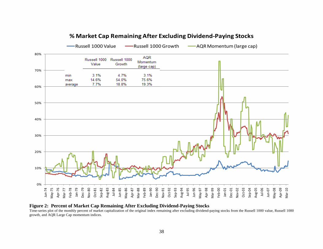
38

Figure 2: Percent of Market Cap Remaining After Excluding Dividend-Paying Stocks Time-series plot of the monthly percent of market capitalization of the original index remaining after excluding dividend-paying stocks from the Russell 1000 value, Russell 1000 growth, and AQR Large Cap momentum indices.

0%

10%

20%

30%

40%

50%

60%

70%

80%

Jun-

74

May

-75

Apr-

76

Mar

-77

Feb-

78

Jan-

79

Dec-

79

Nov-

80

Oct-8

1

Sep-

82

Aug-

83

Jul-8

4

Jun-

85

May

-86

Apr-

87

Mar

-88

Feb-

89

Jan-

90

Dec-

90

Nov-

91

Oct-9

2

Sep-

93

Aug -

94

Jul-9

5

Jun-

96

May

-97

Apr-

98

Mar

-99

Feb-

00

Jan-

01

Dec-

01

Nov-

02

Oct-0

3

Sep-

04

Aug-

05

Jul-0

6

Jun-

07

May

-08

Apr-

09

Mar

-10

% Market Cap Remaining After Excluding Dividend-Paying StocksRussell 1000 Value Russell 1000 Growth AQR Momentum (large cap)

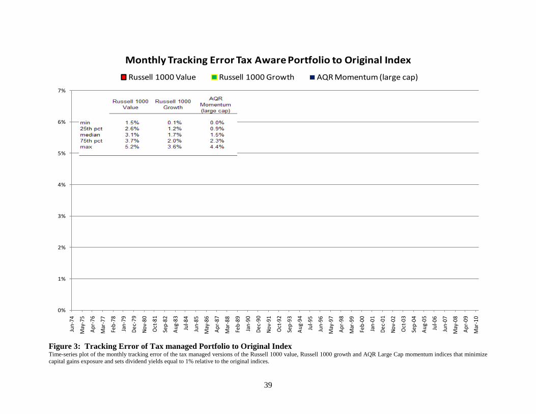
39

Figure 3: Tracking Error of Tax managed Portfolio to Original Index Time-series plot of the monthly tracking error of the tax managed versions of the Russell 1000 value, Russell 1000 growth and AQR Large Cap momentum indices that minimize capital gains exposure and sets dividend yields equal to 1% relative to the original indices.

0%

1%

2%

3%

4%

5%

6%

7%

Jun-

74

May

-75

Apr-

76

Mar

-77

Feb-

78

Jan-

79

Dec-

79

Nov-

80

Oct

-81

Sep-

82

Aug-

83

Jul-8

4

Jun-

85

May

-86

Apr-

87

Mar

-88

Feb-

89

Jan-

90

Dec-

90

Nov-

91

Oct

-92

Sep-

93

Aug-

94

Jul-9

5

Jun-

96

May

-97

Apr-

98

Mar

-99

Feb-

00

Jan-

01

Dec -

01

Nov-

02

Oct

-03

Sep-

04

Aug-

05

Jul-0

6

Jun-

07

May

-08

Apr-

09

Mar

-10

Monthly Tracking Error Tax Aware Portfolio to Original IndexRussell 1000 Value Russell 1000 Growth AQR Momentum (large cap)

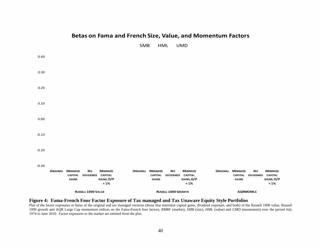
40

Figure 4: Fama-French Four Factor Exposure of Tax managed and Tax Unaware Equity Style Portfolios Plot of the factor exposures or betas of the original and tax managed versions (those that minimize capital gains, dividend exposure, and both) of the Russell 1000 value, Russell 1000 growth and AQR Large Cap momentum indices on the Fama-French four factors, RMRF (market), SMB (size), HML (value) and UMD (momentum) over the period July 1974 to June 2010. Factor exposures to the market are omitted from the plot.

-0.30

-0.20

-0.10

0.00

0.10

0.20

0.30

0.40

ORIGINAL MINIMIZECAPITAL

GAINS

NODIVIDENDS

MINIMIZECAPITAL

GAINS, D/P = 1%

ORIGINAL MINIMIZECAPITAL

GAINS

NODIVIDENDS

MINIMIZECAPITAL

GAINS, D/P = 1%

ORIGINAL MINIMIZECAPITAL

GAINS

NODIVIDENDS

MINIMIZECAPITAL

GAINS, D/P = 1%

RUSSELL 1000 VALUE RUSSELL 1000 GROWTH AQRMOMLC

Betas on Fama and French Size, Value, and Momentum FactorsSMB HML UMD

41

Figure 5: After-Tax Excess Market Returns of value, growth, and momentum Plotted are the average annualized after-tax excess returns of the Russell 1000 value, Russell 1000 growth, and AQR Large Cap momentum portfolios for the original indices, tax managed portfolios that minimize capital gains exposure, tax managed portfolios that eliminate all dividend paying stocks and tax managed portfolios that minimize capital gains subject to a dividend yield of 1%. After-tax returns are calculated assuming 2011 tax rates and are reported as both stand-alone investments that assume carry-forward losses and within a broader portfolio that assumes all losses are available for immediate use.

0.52% 0.52% 0.63% 0.60%

-0.52% -0.51%

1.06% 1.09%

-1.56%-1.37%

-1.53%-1.36%

-0.64%-0.50%

-1.19%-1.04%

0.60%

1.72%

0.71%

1.78%2.00%

3.34%

1.30%

2.23%

-2.00%

-1.00%

0.00%

1.00%

2.00%

3.00%

4.00%

Stand-alone Within a portfolio

Stand-alone Within a portfolio

Stand-alone Within a portfolio

Stand-alone Within a portfolio

Original portfolio Minimize capital gains No dividends Minimize capital gains, D/P=1%

After-Tax Excess Market ReturnsValue Growth Momentum

42

Table 1: After-Tax Returns and Tax Exposures of Long Only Equity Styles

Reported are the annualized average returns before taxes and transaction costs, turnover and dividend yields of the equity portfolios from July 1974 to June 2010 as well as the annualized average after-tax returns, effective tax rates [(before-tax returns - after-tax returns)/before-tax returns] and effective tax rates coming from capital gains and dividend income exposure separately. After-tax returns and tax exposures are computed under two tax regimes: the 2011 tax code and historical tax code lined up contemporaneously with returns in real time. Panel A reports results treating each strategy as a stand-alone investment, where capital losses are netted only against capital gains generated from the portfolio itself and any unused losses are carried forward according to the tax code. Panel B reports results treating each portfolio in the context of a broader portfolio where we assume all losses can be used immediately to offset other gains in the portfolio. All results are presented for an investor at the 99.99th income percentile.

Panel A: CARRYFORWARD LOSSES AS IF A STAND-ALONE INVESTMENTUsing 2011 Tax Rates Using Historical Tax Rates at the time

Annualized before-tax

returnAnnualized

turnoverDividend

yield

Annualized after-tax return

Effective Tax rate

Effective capital gain

tax rate

Effective dividend tax rate

Annualized after-tax return

Effective Tax rate

Effective capital gain

tax rate

Effective dividend tax rate

S&P 500 10.53% 6% 2.8% 9.73% 7.6% 3.2% 4.4% 8.61% 18.2% 4.8% 13.4%Russell 1000 10.66% 7% 2.7% 9.84% 7.7% 3.5% 4.2% 8.74% 18.0% 5.3% 12.7%Russell 1000 Value 12.01% 17% 3.7% 10.36% 13.7% 8.6% 5.1% 8.59% 28.5% 13.1% 15.4%Russell 1000 Growth 8.93% 17% 1.7% 8.28% 7.3% 4.2% 3.1% 7.52% 15.8% 6.5% 9.3%AQR Momentum (large cap) 13.09% 161% 2.1% 10.44% 20.2% 17.6% 2.7% 8.71% 33.5% 25.4% 8.1%MOMLC+R1V 12.82% 90% 2.9% 10.67% 16.8% 13.0% 3.8% 8.93% 30.3% 18.9% 11.5%

MOMLC vs R1V 1.08% 0.08% 0.12%MOMLC vs. R1G 4.17% 2.17% 1.19%MOMLC+R1V vs. R1 2.16% 0.83% 0.19%

Russell 2000 12.00% 27% 1.8% 10.21% 14.9% 12.5% 2.4% 8.81% 26.5% 19.1% 7.5%Russell 2000 Value 13.88% 35% 2.6% 11.32% 18.5% 15.4% 3.1% 9.41% 32.2% 22.8% 9.4%Russell 2000 Growth 9.62% 40% 0.9% 8.25% 14.3% 12.8% 1.5% 7.13% 25.9% 21.0% 4.9%AQR Momentum (small cap) 15.87% 168% 1.2% 12.27% 22.7% 21.4% 1.3% 10.06% 36.6% 32.7% 3.9%MOMSC+R2V 15.20% 103% 2.0% 12.12% 20.3% 18.1% 2.2% 10.03% 34.0% 27.5% 6.6%

MOMSC vs R2V 1.99% 0.95% 0.65%MOMSC vs. R2G 6.25% 4.02% 2.94%MOMSC+R2V vs. R2 3.21% 1.91% 1.22%

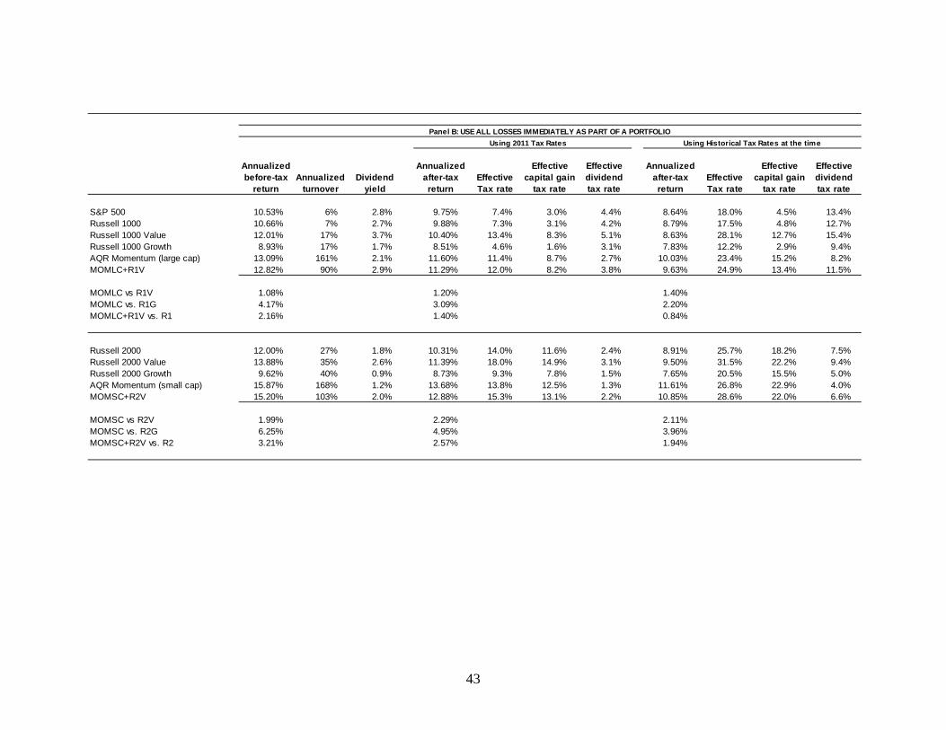
43

Panel B: USE ALL LOSSES IMMEDIATELY AS PART OF A PORTFOLIOUsing 2011 Tax Rates Using Historical Tax Rates at the time

Annualized before-tax

returnAnnualized

turnoverDividend

yield

Annualized after-tax return

Effective Tax rate

Effective capital gain

tax rate

Effective dividend tax rate

Annualized after-tax return

Effective Tax rate

Effective capital gain

tax rate

Effective dividend tax rate

S&P 500 10.53% 6% 2.8% 9.75% 7.4% 3.0% 4.4% 8.64% 18.0% 4.5% 13.4%Russell 1000 10.66% 7% 2.7% 9.88% 7.3% 3.1% 4.2% 8.79% 17.5% 4.8% 12.7%Russell 1000 Value 12.01% 17% 3.7% 10.40% 13.4% 8.3% 5.1% 8.63% 28.1% 12.7% 15.4%Russell 1000 Growth 8.93% 17% 1.7% 8.51% 4.6% 1.6% 3.1% 7.83% 12.2% 2.9% 9.4%AQR Momentum (large cap) 13.09% 161% 2.1% 11.60% 11.4% 8.7% 2.7% 10.03% 23.4% 15.2% 8.2%MOMLC+R1V 12.82% 90% 2.9% 11.29% 12.0% 8.2% 3.8% 9.63% 24.9% 13.4% 11.5%

MOMLC vs R1V 1.08% 1.20% 1.40%MOMLC vs. R1G 4.17% 3.09% 2.20%MOMLC+R1V vs. R1 2.16% 1.40% 0.84%

Russell 2000 12.00% 27% 1.8% 10.31% 14.0% 11.6% 2.4% 8.91% 25.7% 18.2% 7.5%Russell 2000 Value 13.88% 35% 2.6% 11.39% 18.0% 14.9% 3.1% 9.50% 31.5% 22.2% 9.4%Russell 2000 Growth 9.62% 40% 0.9% 8.73% 9.3% 7.8% 1.5% 7.65% 20.5% 15.5% 5.0%AQR Momentum (small cap) 15.87% 168% 1.2% 13.68% 13.8% 12.5% 1.3% 11.61% 26.8% 22.9% 4.0%MOMSC+R2V 15.20% 103% 2.0% 12.88% 15.3% 13.1% 2.2% 10.85% 28.6% 22.0% 6.6%

MOMSC vs R2V 1.99% 2.29% 2.11%MOMSC vs. R2G 6.25% 4.95% 3.96%MOMSC+R2V vs. R2 3.21% 2.57% 1.94%

44

Table 2: Short and Long-Term Capital Gain and Loss Exposure of Equity Styles

Reported are the annualized turnover, long and short-term gains and losses as a percent of the net asset value of each style (per $), percentage of long-term gains and short-term losses realized and the average loss carry-forward (unused losses) per year as a percent of net asset value for each index under the 2011 U.S. tax code.

% NAV Gains and Losses

Annualized turnover

Long-term gains

Short-term gains

Long-term losses

Short-term losses

% Long-term gains

% Short-term losses

Average loss carryforward

(%NAV)

S&P 500 6% 2.50% 0.09% 0.54% 0.10% 97.6% 9.5% 0.1%Russell 1000 7% 2.77% 0.19% 0.68% 0.24% 96.1% 21.4% 0.3%Russell 1000 Value 17% 5.13% 1.07% 1.01% 0.30% 85.4% 19.6% 0.4%Russell 1000 Growth 17% 3.93% 0.51% 1.59% 1.16% 90.9% 44.0% 3.3%AQR Momentum (large cap) 161% 7.74% 9.89% 0.24% 10.35% 45.9% 96.8% 6.2%MOMLC+R1V 90% 6.41% 5.39% 0.83% 5.16% 58.2% 81.1% 2.3%

Russell 2000 27% 8.60% 2.45% 2.88% 1.34% 79.1% 30.4% 0.3%Russell 2000 Value 35% 8.16% 4.16% 2.62% 1.35% 67.6% 31.1% 0.5%Russell 2000 Growth 40% 9.27% 3.81% 4.07% 4.14% 69.6% 48.2% 5.8%AQR Momentum (small cap) 168% 8.51% 17.72% 0.32% 16.53% 29.1% 97.5% 6.0%MOMSC+R2V 103% 8.93% 10.63% 1.95% 8.71% 45.6% 79.2% 2.3%

45

Table 3: After-Tax Returns in Up and Down Markets When Losses Can Be Used Immediately

Reported are the pre-tax and after-tax average returns, as well as the difference between them, of each of the equity styles under the 2011 U.S. tax code. After-tax returns assume all losses can be used immediately in a portfolio context. The first three columns report mean returns in up market environments only, defined as years for which the Russell 1000 delivered a positive return (1975-1976,1978-1980, 1982-1989, 1991-1993, 1995-1999, 2003-2007 and 2009), the second three columns reports results in down markets only, defined as years for which the Russell 1000 delivered a negative return (1981, 1990, 1994, 2000-2002 and 2008) and the last three columns reports results for the recent financial crisis from July 2007 to March 2009.

Up Markets Down Markets July 2007 to March 2009

Pre-tax mean return

After-tax mean return Difference

Pre-tax mean return

After-tax mean return Difference

Pre-tax mean return

After-tax mean return Difference

S&P 500 18.76% 18.00% -0.76% -14.84% -15.41% -0.57% -30.78% -30.98% -0.20%Russell 1000 18.83% 18.05% -0.77% -14.49% -14.99% -0.49% -30.48% -30.87% -0.38%Russell 1000 Value 18.63% 17.10% -1.53% -8.91% -10.12% -1.20% -35.99% -36.64% -0.65%Russell 1000 Growth 18.94% 18.42% -0.53% -20.29% -20.21% 0.07% -25.17% -25.40% -0.23%AQR Momentum (large cap) 22.56% 19.57% -3.00% -15.34% -11.26% 4.08% -27.77% -19.49% 8.27%MOMLC+R1V 20.77% 18.53% -2.24% -12.24% -10.83% 1.41% -32.11% -28.47% 3.64%

MOMLC vs R1V 3.93% 2.47% -6.43% -1.15% 8.23% 17.14%MOMLC vs. R1G 3.62% 1.15% 4.95% 8.95% -2.60% 5.90%MOMLC+R1V vs. R1 1.94% 0.47% 2.25% 4.16% -1.63% 2.39%

Russell 2000 19.58% 17.89% -1.69% -8.87% -9.85% -0.99% -32.11% -32.89% -0.78%Russell 2000 Value 19.44% 17.08% -2.36% -2.28% -4.08% -1.81% -34.19% -34.65% -0.46%Russell 2000 Growth 19.43% 18.28% -1.15% -15.41% -15.12% 0.29% -29.97% -30.27% -0.30%AQR Momentum (small cap) 24.21% 20.77% -3.44% -6.23% -2.97% 3.26% -34.30% -22.30% 12.00%MOMSC+R2V 22.13% 19.26% -2.87% -4.37% -3.71% 0.66% -34.88% -28.96% 5.92%

MOMSC vs R2V 4.76% 3.69% -3.95% 1.11% -0.11% 12.35%MOMSC vs. R2G 4.77% 2.49% 9.19% 12.15% -4.33% 7.98%MOMSC+R2V vs. R2 2.55% 1.37% 4.49% 6.14% -2.77% 3.93%

46

Table 4: After-Tax Returns and Tax Exposures of Equity Portfolios from 1927 to 2010

Panel A reports the annualized average before-tax and after-tax returns and effective tax rates of the academic portfolios from Bergstresser and Pontiff (2011), which cover the period June 1927 to June 2007. Panel B reports results for the same portfolios updated through June 2010. After-tax returns and tax exposures are computed under two tax regimes: the 2000 U.S. tax code and the historical tax code lined up contemporaneously with returns in real time. Losses are assumed to be available for immediate use in the context of a broader portfolio.

PANEL A: BERGSTRESSER AND PONTIFF (2009) JUNE 1927 TO JUNE 2007

Using 2000 Tax Rates Using Historical Tax RatesAnnualized before-tax

return

Annualized after-tax return

Effective tax rate

Annualized after-tax return

Effective tax rate

Market 9.79% 7.95% 18.8% 7.08% 27.7%Value 12.63% 9.93% 21.4% 8.24% 34.8%Growth 8.86% 7.36% 16.9% 6.49% 26.7%Momentum 14.04% 10.51% 25.2% 8.53% 39.3%MOM + VAL 13.34% 10.22% 23.3% 8.39% 37.0%

MOM vs VAL 1.41% 0.58% 0.29%MOM vs GRO 5.18% 3.15% 2.04%MOM+VAL vs Market 3.55% 2.27% 1.31%

PANEL B: UPDATED JUNE 1927 TO JUNE 2010

Using 2000 Tax Rates Using Historical Tax RatesAnnualized before-tax

return

Annualized after-tax return

Effective tax rate

Annualized after-tax return

Effective tax rate

Market 9.04% 7.26% 19.6% 6.43% 28.9%Value 11.63% 9.03% 22.3% 7.42% 36.2%Growth 8.26% 6.83% 17.3% 6.00% 27.4%Momentum 13.02% 9.81% 24.6% 7.92% 39.2%MOM + VAL 12.33% 9.43% 23.5% 7.68% 37.7%

MOM vs VAL 1.39% 0.78% 0.50%MOM vs GRO 4.76% 2.98% 1.92%MOM+VAL vs Market 3.30% 2.17% 1.25%

47

Table 5: Tax Managed Equity Style Portfolios---Capital Gains Exposure

Reported are results based on the 2011 tax code from tax-optimized or "tax managed" portfolios of the equity indices by minimizing capital gains tax exposure subject to a tracking error constraint that requires use of an ex ante risk model. Panel A reports results that use the one-month lagged USE3S BARRA risk model (US Short-Term model) to estimate ex ante tracking error, and Panel B reports results that use the Fama and French four factor model to estimate ex ante tracking error (using rolling five year beta estimates and covariance matrices). Ex ante tracking error is constrained to be less than 25 basis points for the large cap and the small cap portfolios. In both panels, the annualized average after-tax returns and effective tax rates of the tax managed portfolios are reported along with their differences from the original indices (that are not tax managed). Also reported is the change in turnover, long-term gains, and short-term losses between the tax managed versions and original indices. The last three columns report the alpha, t-stat of alpha and ex post tracking error from a time-series regression of the tax managed portfolios on the original indices.

Regression On Original PortfolioAfter-tax

return∆ from original

Effective tax rate

∆ from original ∆ Turnover

∆ Long-term gains

∆ Short-term losses Alpha

T-stat of alpha Tracking error

Panel A: TRACKING ERROR ESTIMATED FROM BARRA USE3S RISK MODEL

S&P 500 9.95% 0.22% 6.8% -0.9% 17% -10.5% 59.7% 0.24% (3.74) 0.35%Russell 1000 10.05% 0.21% 6.7% -1.0% 2% -2.0% 15.0% 0.19% (2.69) 0.38%Russell 1000 Value 10.68% 0.32% 11.0% -2.7% -4% 7.1% 5.1% 0.33% (2.95) 0.59%Russell 1000 Growth 8.52% 0.25% 5.9% -1.4% -1% 3.1% 7.2% 0.25% (2.26) 0.58%AQR Momentum (large cap) 10.77% 0.32% 16.9% -3.4% -20% 8.7% -0.3% 0.22% (1.99) 0.59%MOMLC+R1V 11.09% 0.42% 13.3% -3.5% -10% 10.7% 3.8% 0.28% (3.30) 0.45%

Russell 2000 10.40% 0.19% 14.1% -0.8% 7% -5.5% 8.2% 0.14% (0.92) 0.81%Russell 2000 Value 11.92% 0.60% 14.9% -3.6% -3% 7.0% 7.7% 0.54% (3.58) 0.81%Russell 2000 Growth 8.29% 0.04% 14.2% -0.1% 3% -1.8% 4.0% -0.03% (-0.16) 1.02%AQR Momentum (small cap) 12.46% 0.18% 20.3% -2.4% -11% 3.9% -0.7% 0.06% (0.45) 0.68%MOMSC+R2V 12.73% 0.62% 16.0% -4.3% -4% 5.6% 6.5% 0.39% (3.29) 0.64%

Panel B: TRACKING ERROR ESTIMATED FROM FAMA-FRENCH 4-FACTOR MODEL

S&P 500 9.96% 0.27% 7.0% -1.2% 12% -9.3% 58.4% 0.31% (3.27) 0.51%Russell 1000 9.93% 0.15% 7.3% -0.9% 2% -1.0% 21.5% 0.06% (0.55) 0.55%Russell 1000 Value 10.65% 0.37% 11.3% -2.8% -4% 5.3% 7.0% 0.27% (1.71) 0.85%Russell 1000 Growth 8.38% 0.14% 6.5% -1.2% -2% 2.6% 5.4% 0.17% (1.25) 0.72%AQR Momentum (large cap) 10.74% 0.29% 17.0% -3.3% -22% 8.5% -0.3% 0.20% (1.39) 0.78%MOMLC+R1V 11.18% 0.54% 12.6% -4.4% -15% 7.8% 6.3% 0.33% (2.77) 0.65%

Russell 2000 10.72% 0.15% 13.8% -1.0% 8% -4.6% 7.0% 0.43% (1.96) 1.19%Russell 2000 Value 12.33% 0.79% 14.4% -3.8% -2% 5.8% 9.1% 0.84% (4.00) 1.13%Russell 2000 Growth 8.74% 0.08% 14.4% -0.1% 2% -1.7% 2.5% 0.39% (1.47) 1.43%AQR Momentum (small cap) 12.55% 0.06% 20.4% -2.5% -13% 3.7% -1.6% 0.03% (0.18) 1.00%MOMSC+R2V 13.33% 1.02% 15.1% -5.0% -5% 5.2% 9.8% 0.93% (5.45) 0.91%

48

Table 6: Tax Managed Equity Style Portfolios---Dividend Exposure

Reported are results based on the 2011 tax code from tax-optimized or "tax managed" portfolios of the equity indices by minimizing dividend exposure. Panel A simply excludes all dividend paying stocks. Panel B minimizes the dividend yield of the portfolio subject to a tracking error constraint (using the one-month lagged USE3S BARRA risk model to estimate ex ante tracking error). Panel C sets the dividend yield of the portfolio equal to 1% and minimizes tracking error. Panel D sets the dividend yield to 1% and minimizes both tracking error and capital gains exposure. All panels report the annualized average after-tax returns, effective tax rates and dividend yields of the tax managed portfolios, along with their differences from the original indices (that are not tax managed). Also reported is the ex post tracking error from a time-series regression of the tax managed portfolio on the original index.

After-tax return

∆ from original

Effective tax rate

∆ from original Dividend yield

∆ from original Tracking error

Panel A: EXCLUDE ALL DIVIDEND-PAYING STOCKS

S&P 500 10.19% 0.47% 9.5% 1.8% 0.0% -2.8% 11.76%Russell 1000 10.08% 0.24% 9.0% 1.4% 0.0% -2.7% 10.10%Russell 1000 Value 9.56% -0.80% 18.5% 4.8% 0.1% -3.7% 10.22%Russell 1000 Growth 9.44% 1.16% 8.0% 0.8% 0.0% -1.7% 8.87%AQR Momentum (large cap) 12.08% 1.63% 18.5% -1.8% 0.0% -2.1% 10.10%MOMLC+R1V 11.90% 1.22% 17.1% 0.4% 0.0% -2.9% 10.42%

Panel B: MINIMIZE DIVIDEND YIELD SUBJECT TO TRACKING ERROR CONSTRAINT

S&P 500 9.70% -0.02% 7.7% 0.1% 2.8% 0.0% 0.17%Russell 1000 9.60% -0.24% 8.8% 1.2% 2.5% -0.3% 0.72%Russell 1000 Value 10.14% -0.22% 14.7% 0.9% 3.4% -0.4% 0.84%Russell 1000 Growth 8.28% 0.00% 7.2% 0.0% 1.7% 0.0% 0.46%AQR Momentum (large cap) 10.44% -0.01% 20.3% 0.1% 2.1% 0.0% 0.32%MOMLC+R1V 10.55% -0.12% 17.2% 0.4% 2.7% -0.3% 0.38%

49

After-tax return

∆ from original

Effective tax rate

∆ from original Dividend yield

∆ from original Tracking error

Panel C: DIVIDEND YIELD = 1%, MINIMIZE TRACKING ERROR

S&P 500 9.45% -0.28% 13.2% 5.6% 1.0% -1.8% 2.62%Russell 1000 8.84% -1.00% 10.9% 3.2% 1.0% -1.7% 2.27%Russell 1000 Value 9.27% -1.10% 14.9% 1.2% 1.0% -2.7% 3.21%Russell 1000 Growth 8.04% -0.24% 8.9% 1.7% 0.9% -0.7% 1.95%AQR Momentum (large cap) 10.50% 0.06% 19.5% -0.8% 0.9% -1.2% 1.76%MOMLC+R1V 10.26% -0.41% 18.4% 1.6% 1.0% -1.9% 2.09%

Panel D: DIVIDEND YIELD = 1%, MINIMIZE TRACKING ERROR AND MINIMIZE CAPITAL GAIN

S&P 500 10.49% 0.77% 6.5% -1.1% 1.0% -1.8% 2.96%Russell 1000 9.77% -0.07% 5.6% -2.1% 1.0% -1.7% 2.47%Russell 1000 Value 10.83% 0.47% 6.7% -7.0% 1.0% -2.7% 3.56%Russell 1000 Growth 8.57% 0.29% 5.1% -2.1% 0.9% -0.8% 2.03%AQR Momentum (large cap) 11.07% 0.62% 11.8% -8.4% 0.9% -1.2% 2.12%MOMLC+R1V 11.01% 0.34% 12.7% -4.1% 1.0% -1.9% 2.20%

50

Appendix

Table A1: Correlations between Replicated and Actual Indices Reported are the return correlations between actual indices versus replicated indices over the overlapping live period of the actual index returns. For the purposes of the correlation analysis below, we extended the replicated indices to the live period. We report the return correlation of each index to its replicated version.

Correlation Correlation

Russell 1000 0.989 Russell 2000 0.956Russell 1000 Value 0.982 Russell 2000 Value 0.967Russell 1000 Growth 0.989 Russell 2000 Growth 0.923AQR Momentum (large cap) 0.997 AQR Momentum (small cap) 0.995

Large cap indices Small cap indices

51

Table A2: Historical Tax Rates Tax rates by year for an investor in the 95th and 99.99th income percentile of the U.S. tax code from 1974 to 2011. Tax rates are obtained from the Federal Individual Income Tax Rates History 1913 - 2011 from the Tax Foundation in Washington, D.C. and from the Department of the Treasury, Office of Tax Analysis (November 3, 2008).

Tax Rates by Year (99.99th income percentile)

Tax Rates by Year (95th income percentile)

YearShort-term

rate (%)Long-term

rate (%)Dividend

income (%)Short-term

rate (%)Long-term

rate (%)Dividend

income (%)1974 70.0 36.5 70.0 45.0 36.5 45.01975 70.0 36.5 70.0 45.0 36.5 45.01976 70.0 39.9 70.0 45.0 39.9 45.01977 70.0 39.9 70.0 45.0 39.9 45.01978 70.0 39.9 70.0 50.0 39.9 50.01979 70.0 28.0 70.0 49.0 28.0 49.01980 70.0 28.0 70.0 55.0 28.0 55.01981* 70.0 20.0 70.0 55.0 20.0 55.01982 50.0 20.0 50.0 50.0 20.0 50.01983 50.0 20.0 50.0 45.0 20.0 45.01984 50.0 20.0 50.0 42.0 20.0 42.01985 50.0 20.0 50.0 48.0 20.0 48.01986 50.0 20.0 50.0 48.0 20.0 48.01987 38.5 28.0 38.5 38.5 28.0 38.51988 28.0 28.0 28.0 33.0 28.0 33.01989 28.0 28.0 28.0 33.0 28.0 33.01990 28.0 28.0 28.0 33.0 28.0 33.01991 31.0 28.0 31.0 31.0 28.0 31.01992 31.0 28.0 31.0 31.0 28.0 31.01993 39.6 28.0 39.6 31.0 28.0 31.01994 39.6 28.0 39.6 31.0 28.0 31.01995 39.6 28.0 39.6 31.0 28.0 31.01996 39.6 28.0 39.6 31.0 28.0 31.01997* 39.6 20.0 39.6 31.0 20.0 31.01998 39.6 20.0 39.6 31.0 20.0 31.01999 39.6 20.0 39.6 31.0 20.0 31.02000 39.6 20.0 39.6 31.0 20.0 31.02001 39.1 20.0 39.1 31.0 20.0 31.02002 38.6 20.0 38.6 30.0 20.0 30.02003* 35.0 15.0 15.0 28.0 15.0 15.02004 35.0 15.0 15.0 28.0 15.0 15.02005 35.0 15.0 15.0 28.0 15.0 15.02006 35.0 15.0 15.0 28.0 15.0 15.02007 35.0 15.0 15.0 28.0 15.0 15.02008 35.0 15.0 15.0 28.0 15.0 15.02009 35.0 15.0 15.0 28.0 15.0 15.02010 35.0 15.0 15.0 28.0 15.0 15.02011 35.0 15.0 15.0 28.0 15.0 15.0*Mid-year rate changes

52

Table A3: After-Tax Returns for Investors at Different Income Percentiles

Reported are the annualized average returns after taxes but before transaction costs of the equity portfolios from July 1974 to June 2010 for investors at the 99.99th and 95th income percentiles. After-tax returns and tax exposures are computed under two tax regimes: the 2011 tax code and historical tax code lined up contemporaneously with returns in real time. Each strategy is treated as a stand-alone investment.

Using 2011 Tax RatesUsing Historical Tax Rates at

the time

99.99th Percentile

95th Percentile

99.99th Percentile

95th Percentile

S&P 500 9.73% 9.73% 8.61% 8.86%Russell 1000 9.84% 9.85% 8.74% 8.99%Russell 1000 Value 10.36% 10.43% 8.59% 9.00%Russell 1000 Growth 8.28% 8.29% 7.52% 7.67%AQR Momentum (large cap) 10.44% 10.73% 8.71% 9.22%MOMLC+R1V 10.67% 10.86% 8.93% 9.38%

MOMLC vs R1V 0.08% 0.31% 0.12% 0.23%MOMLC vs. R1G 2.17% 2.44% 1.19% 1.55%MOMLC+R1V vs. R1 0.83% 1.01% 0.19% 0.40%

Russell 2000 10.21% 10.32% 8.81% 9.15%Russell 2000 Value 11.32% 11.54% 9.41% 9.99%Russell 2000 Growth 8.25% 8.34% 7.13% 7.39%AQR Momentum (small cap) 12.27% 12.77% 10.06% 10.90%MOMSC+R2V 12.12% 12.47% 10.03% 10.72%

MOMSC vs R2V 0.95% 1.22% 0.65% 0.92%MOMSC vs. R2G 4.02% 4.42% 2.94% 3.51%MOMSC+R2V vs. R2 1.91% 2.15% 1.22% 1.57%

Annualized after-tax return