the journal of - home | institutional investor 015 the journal of investing sample (in fact,...

T H E J O U R N A L O F

The Voices of Influence | iijournals.com

SUMMER 2015 Volume 24 Number 2 THEORY & PRACTICE FOR FUND MANAGERS

Working Your Tail off: Active StrAtegieS verSuS Direct HeDging Summer 2015

Working Your Tail Off: Active Strategies Versus Direct HedgingAttAkrit AsvAnunt, LArs n. nieLsen, And dAnieL viLLALon

AttAkrit AsvAnunt

is a vice president at AQR Capital Management in Greenwich, [email protected]

LArs n. nieLsen

is a principal at AQR Capital Management in Greenwich, [email protected]

DAnieL viLLALon

is a vice president at AQR Capital Management in Greenwich, [email protected]

One of the main financial stories over the past f ive years is tail risk. However, though it’s clear that most traditional portfolios

have it, it’s far less clear what to do about it. Complicating matters, by definition, tail events offer researchers very few data points, and even the definition of a tail event is not standardized.

Despite these challenges, most investors can be reasonably confident about where their portfolio’s tail risk comes from: equities. Though a 60% equity and 40% bond portfolio may appear reasonably diversified in terms of capital, when viewed by risk, the 60/40 portfolio over the long term looks more like 90/10. This is because equities are a riskier asset class than bonds—since 1903 the volatility of U.S. equities has been 18.0% versus 5.8% for U.S. bonds.1 Though any asset class has tail risk, for the majority of investors, equity tail risk is the one that matters most.

This study compares two basic approaches for hedging the equity tails of a U.S. 60/40 portfolio:2 1) the direct approach, which uses option markets to hedge the equity component of the starting portfolio, and 2) the indirect approach, which instead seeks to alter the starting portfolio. For the direct approach, we evaluate a collar strategy, which partially f inances long positions in outofthemoney puts by selling outofthe

money calls.3 Within the indirect approach, we consider three strategies, each of which is constrained to U.S. stocks and bonds, so as not to introduce effects from diversification to other asset classes and countries:

1. Reducing equity risk within the equity allocation.

2. Altering the stock/bond allocation.3. Incorporating a trendbased rebalancing

strategy.

These three strategies were chosen because they have empirically shown a tendency to mitigate or hedge equity market drawdowns without requiring unique timing ability and, in contrast to direct insurance, have historically delivered positive realized returns. Additionally, each of these strategies, on average, has long exposure to one or more wellknown market risk premia (for example, stocks and bonds) or style premia (for example, trendfollowing and lowrisk investing), so it is reasonable to believe that they have a positive longterm expected return. Finally, these strategies are straightforward to define and construct.

Over the full period for which we have options data, 1985–2012, the average performance of the direct and indirect approaches is meaningfully different. Compared with the starting 60/40 portfolio, the directhedged portfolio did not add value over the full

The Journal of InvesTIngSummer 2015

sample (in fact, detracted, albeit by a statistically insignificant level). In contrast, each of the three indirect approaches (alternative portfolios) generated positive and signif icant alpha in regressions to the starting 60/40 portfolio. Still, there is a tradeoff: though the indirect approaches have added value over the longer term, they are not guaranteed to do so in short, sharp crashes.

Over the worst peaktotrough drawdowns, we f ind that while the direct optionsbased approaches provide protection from sudden, large losses in equities, those gains are eroded in subsequent periods at a fasterthanaverage rate. We find comparable performance between direct and indirect hedging approaches over the worst multiplemonth equity drawdowns since 1985, and meaningful outperformance outside of those periods for the indirect approaches. Though the direct, optionsbased approach may deliver in the short term, to profit from it requires timing ability not only to purchase protection before a bad event but also to take it off before gains are eroded.

For many investors, indirect approaches may represent a better choice for capturing insurancelike returns at a lower cost. Though the alternatives proposed in this article all require some form of skill to implement, they don’t require magic.

DATA AND APPROACH

In order to examine the costs and benef its of directhedging strategies, we build a collar strategy using Standard & Poor’s 100 options from 1985–1995 and Standard & Poor’s 500 options from 1996–2012.4,5

The returns from options strategies are highly pathdependent—for example, the returns for a strategy that holds a singlestrike put option will be dependent not just on the magnitude of losses but also on where the losses start from relative to the strike. To reduce the likelihood of spurious findings, we hold overlapping threemonth put options, so that at all times there are three options expiring one, two, or three months in the future, thus creating an insurance portfolio with a more stable maturity profile. The other side of the directhedging strategy is to sell onemonth call options. The reason for the different maturities between the put and call is twofold: 1) from a tailhedging perspective, the payoff structure of long threemonth puts and short onemonth calls is empirically more attractive than with matching maturities (that is, it produces a reasonably convex payoff

relative to returns of stocks), and 2) it is similar to the construction of popular collar indexes, most notably the CBOE S&P 500 95–110 Collar Index (CLL).6

Strikes are another parameter for options. Our collar strategy is 92.5–110, meaning the put options are 7.5% outofthemoney and the call options are 10% outofthemoney. Though the choice of strike is somewhat arbitrary (for example, it depends from investor to investor on desired level of portfolio protection), anecdotal evidence across a range of investor types suggests that 92.5–110 is a reasonably representative collar strategy.

We compare the directhedging strategy (the collar) with three indirect strategies, each of which has an economic rationale and decades of empirical evidence for mitigating tail events of 60/40 portfolios. We constrain these indirect strategies to include only U.S. stocks and/or bonds, which maintains the same number of asset classes as in the starting 60/40 portfolio and limits diversif ication benefits that adding a new asset class may bring. These indirect strategies are combined with the starting 60/40 portfolio to build alternative portfolios, as follows:

Reducing Equity Risk Within the Equity Allocation: Low-Beta EquitiesDescription. Lowbeta stock selection7 seeks

to capture returns from the lowbeta anomaly, which finds that lowerbeta stocks tend to have higher returns than predicted by standard one, three, and fourfactor asset pricing models.8 In contrast to reducing equity risk by reducing the capital allocated to equities, this portfolio instead overweights stocks with low market betas and underweights stocks with high market betas, thus reducing the portfolio’s beta while remaining fully invested in equity markets. The alternative portfolio we evaluate replaces the starting 60/40 portfolio’s entire capitalizationweighted stock allocation with lowbeta stocks.

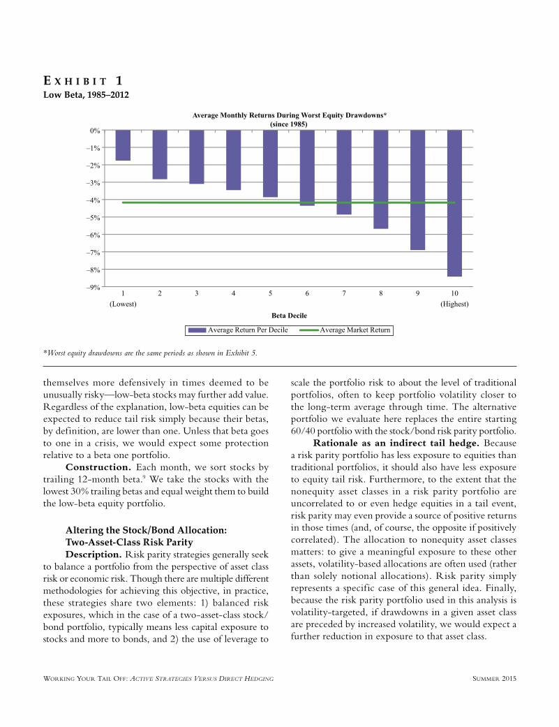
Rationale as an indirect tail hedge. Lowbeta investing reduces the amount of equity tail risk in a portfolio primarily by reducing the portfolio’s beta (as shown in Exhibit 1). To the extent that there is the lowbeta premium during tail events—for example, if investors sell higherbeta, riskier stocks in favor of lowerbeta, safer stocks in an equity drawdown, or if benchmarkoriented equity managers seek to position


themselves more defensively in times deemed to be unusually risky—lowbeta stocks may further add value. Regardless of the explanation, lowbeta equities can be expected to reduce tail risk simply because their betas, by definition, are lower than one. Unless that beta goes to one in a crisis, we would expect some protection relative to a beta one portfolio.

Construction. Each month, we sort stocks by trailing 12month beta.9 We take the stocks with the lowest 30% trailing betas and equal weight them to build the lowbeta equity portfolio.

Altering the Stock/Bond Allocation: Two-Asset-Class Risk ParityDescription. Risk parity strategies generally seek

to balance a portfolio from the perspective of asset class risk or economic risk. Though there are multiple different methodologies for achieving this objective, in practice, these strategies share two elements: 1) balanced risk exposures, which in the case of a twoassetclass stock/bond portfolio, typically means less capital exposure to stocks and more to bonds, and 2) the use of leverage to

scale the portfolio risk to about the level of traditional portfolios, often to keep portfolio volatility closer to the longterm average through time. The alternative portfolio we evaluate here replaces the entire starting 60/40 portfolio with the stock/bond risk parity portfolio.

Rationale as an indirect tail hedge. Because a risk parity portfolio has less exposure to equities than traditional portfolios, it should also have less exposure to equity tail risk. Furthermore, to the extent that the nonequity asset classes in a risk parity portfolio are uncorrelated to or even hedge equities in a tail event, risk parity may even provide a source of positive returns in those times (and, of course, the opposite if positively correlated). The allocation to nonequity asset classes matters: to give a meaningful exposure to these other assets, volatilitybased allocations are often used (rather than solely notional allocations). Risk parity simply represents a specific case of this general idea. Finally, because the risk parity portfolio used in this analysis is volatilitytargeted, if drawdowns in a given asset class are preceded by increased volatility, we would expect a further reduction in exposure to that asset class.

e x h i b i t 1Low Beta, 1985–2012

*Worst equity drawdowns are the same periods as shown in Exhibit 5.


Construction. The twoassetclass risk parity portfolio seeks to capture equal volatility from the S&P 500 and the Barclays U.S. Treasury Bond Index. Each month, we calculate the trailing 12month volatility of stocks and bonds separately and size a position for the next month to achieve 10% annualized volatility,10 assuming zero correlation between stocks and bonds.11 Exhibit 2 compares the contribution to portfolio risk in the starting 60/40 portfolio and the twoassetclass risk parity portfolio.

Incorporating a Trend-Based Rebalancing Strategy: Trend Following12

Description. Historically, when equities have suffered prolonged declines, trendfollowing strategies have, not surprisingly, done well. Our third alternative is a twoasset, longshort, trendfollowing strategy using the S&P 500 and the Barclays U.S. Treasury Bond Index.13 Our alternative portfolio replaces 20% of the starting portfolio with this trendfollowing strategy.14

Rationale as an indirect tail hedge. Most bear markets do not happen overnight but instead occur as the result of prolonged economic deterioration. Trendfollowing strategies position themselves short as markets begin to decline and can profit if markets continue to fall. Because price trends can be positive or negative, trendfollowing portfolios—unlike many other investments

in institutional portfolios—have historically delivered strong performance in both up and down markets (as illustrated in Exhibit 3) and low correlations to markets over the medium to long term.

Construction. This strategy is an equalweighted combination of one, three, and 12month time series momentum strategies. For each of the three time series momentum strategies, the position taken is determined by assessing the past return in that asset over the relevant lookback period. A positive past return is considered an up trend and leads to a long position; a negative past return is considered a down trend and leads to a short position, meaning that stocks and bonds are always either short or long their respective risk premia. Each position is sized to target the same amount of volatility (calculated using trailing 12month returns), and the positions across the three strategies are aggregated each month assuming zero correlation between stocks and bonds and scaled such that the combined portfolio has an annualized ex ante volatility target of 10%.

All of the returns in this analysis are shown gross of transaction costs, which, given the relative illiquidity of options compared to the three indirect alternatives, should provide a relative benef it to the direct tailhedging approach. Additionally, our results for the indirect portfolios are robust to specific design choice—for example, to risk and beta estimation methodologies and trendfollowing parameters.

e x h i b i t 2Two-Asset-Class Risk Parity (1/1985–12/2012)


RESULTS

Comparisons to 60/40

Each of the portfolios in our analysis represents a departure from 60/40. Exhibit 4 highlights the extent of each, comparing the directhedging portfolio and the three alternative portfolios to the starting 60/40. The risk parity portfolio represents the most meaningful

departure—despite investing in the same two assets, its R2 is 0.6 to 60/40 , and its tracking error is 7%. To the extent that investors are less willing to deviate from 60/40, the portfolios that incorporate low beta and trendfollowing approaches may provide more practical choices (or they may consider a smaller allocation to risk parity). Exhibit 4 also highlights that despite the differences across the alternative portfolios, each generated positive and significant alpha to 60/40, whereas the direct hedging portfolio generated negative (though not statistically significant) alpha.

Hedging Effectiveness

We gauge the effectiveness of each approach as a portfolio hedge by examining its performance and total return statistics across various 60/40 drawdown periods, as shown in Exhibit 5. Though neither the direct nor the indirect approaches generated positive portfolio returns during the f ive worst single months, the direct approach generally performed better than the indirect approaches. For example, the direct approach was more effective during the Crash of 1987 and the breakout of the First Gulf War in 1990, when the equity market experienced a severe drawdown over a relatively short time.

However, over the worst peaktotrough drawdowns—most of which include the worst single months—the results are mixed. Direct hedging was much less effective during a protracted drawdown such as that following the DotCom Bust in 2000–2002, as options get repriced and become more expensive during crises. This is consistent with rational pricing—as the demand for protection increases, so

should the price. To the extent that option markets are as efficient as other major, liquid markets, investors should not expect a free lunch in a drawnout crisis.

Over the seven worst equity drawdowns shown in Exhibit 5, the average monthly outperformance of the alternative portfolios was +149 basis points for risk parity, +94 basis points for lowbeta equity and +79 basis points for allocation to trend following, compared

e x h i b i t 4Comparisons to Starting 60/40 Portfolio, 1985–2012

e x h i b i t 3Yearly Returns of Two-Asset Trend Following vs. Equities, 1903–2012


with +71 basis points using direct hedging. Outside of these drawdown periods, the average monthly outperformance of indirect hedging in the alternative portfolios is between +6 basis points and –12 basis points per month, whereas direct hedging was –31 basis points on average, suggesting over the full sample that direct hedging costs 233 basis points to 448 basis points more per year without delivering more protection during these worst drawdowns.

With the exception of risk parity, which targets a f ixed volatility, both the direct and indirect approaches reduce the volatility of the simple 60/40 portfolio, consequently reducing portfolio drawdowns. In the direct approach, however, the reduction of drawdown and volatility comes at a cost of lower riskadjusted returns. Whereas indirect hedging strategies increased the portfolio’s Sharpe ratio, direct hedging did not.

Additional Observations on Each Alternative

Low-beta equities. This strategy had a 0.84 correlation to equities over the full period and averaged a 0.72 beta to equities with 0.26% monthly alpha (2.2 tstat). Despite having a lower beta, the strategy modestly underperformed broad markets in four of the worst five months for equities. Still, low beta outperformed in five of the seven worst multiplemonth drawdowns shown in Exhibit 5, most notably during the DotCom Bust, when lowbeta equities delivered positive returns.

Two-asset-class risk parity. Over the full period, stocks and bonds had a 0.01 correlation and 0.44 and 0.63 Sharpe ratios, respectively. The 60/40 portfolio posted a Sharpe ratio between that of its underlying asset classes, 0.55, whereas the twoassetclass risk parity portfolio benef ited more, generating a 0.79 Sharpe ratio. Furthermore, over the worst individual and multiplemonth drawdowns for equities, bond returns

e x h i b i t 5Standard Statistics of the Portfolios, 1985–2012


outperformed those of equities. Thus, it is not surprising that risk parity outperformed 60/40 during these worst equity periods.15 Granted, because of risk parity’s relative overweight to bonds (compared with 60/40), tail events in bond markets will contribute more to overall portfolio returns than for the 60/40 allocation.16 Even so, the diversification benefit and resulting Sharpe ratio advantage may be considered a source of alpha relative to 60/40.

Trend following. The twoasset, trendfollowing strategy had a 0.07 correlation to stocks over the full period (and a 0.15 correlation to 60/40) and thus contributed some diversification benefit to the starting portfolio. Consistent with f indings in Hurst et al. [2013], the period we study shows negative correlation during negative return months for equities (–0.17 over the 1985–2012 period), suggesting that even a twoasset trendfollowing strategy generates some of the desired nonlinear behavior associated with tail hedges.

Not exchanging one tail for another. Though direct hedging and the indirect alternatives showed the ability to mitigate the worst drawdowns for the 60/40 portfolio, another consideration is whether these approaches introduce new worst drawdowns and, if so, what their magnitudes are relative to those of the starting portfolio.

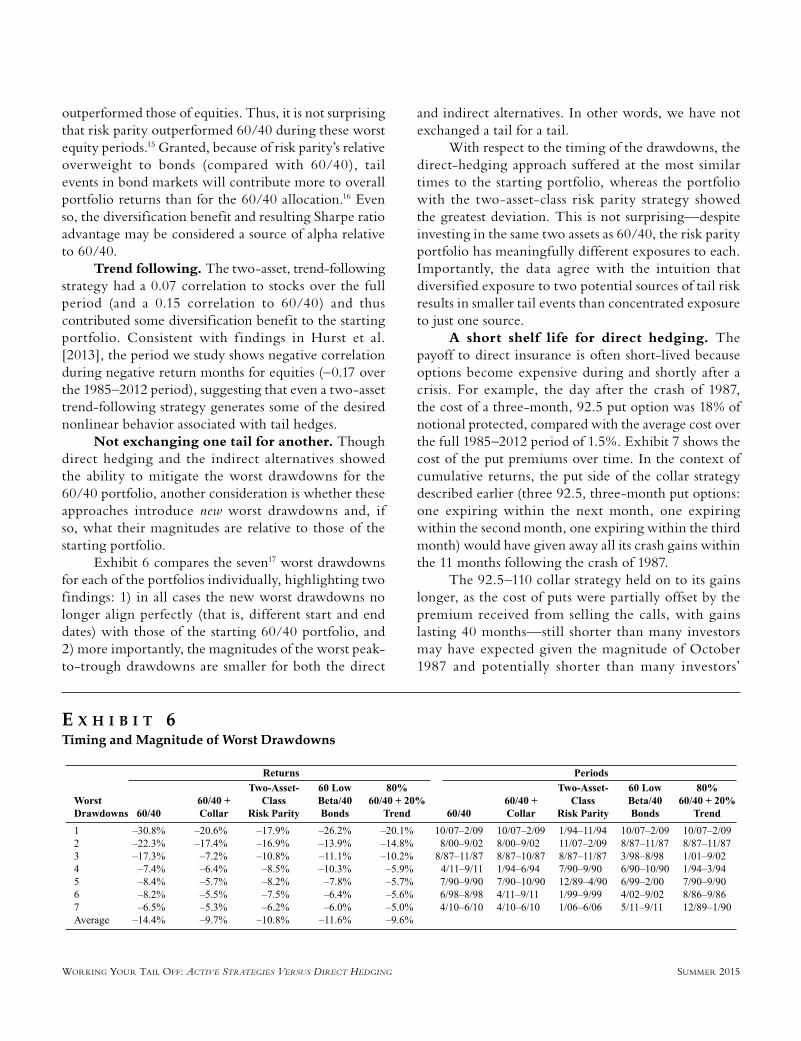
Exhibit 6 compares the seven17 worst drawdowns for each of the portfolios individually, highlighting two findings: 1) in all cases the new worst drawdowns no longer align perfectly (that is, different start and end dates) with those of the starting 60/40 portfolio, and 2) more importantly, the magnitudes of the worst peaktotrough drawdowns are smaller for both the direct

and indirect alternatives. In other words, we have not exchanged a tail for a tail.

With respect to the timing of the drawdowns, the directhedging approach suffered at the most similar times to the starting portfolio, whereas the portfolio with the twoassetclass risk parity strategy showed the greatest deviation. This is not surprising—despite investing in the same two assets as 60/40, the risk parity portfolio has meaningfully different exposures to each. Importantly, the data agree with the intuition that diversified exposure to two potential sources of tail risk results in smaller tail events than concentrated exposure to just one source.

A short shelf life for direct hedging. The payoff to direct insurance is often shortlived because options become expensive during and shortly after a crisis. For example, the day after the crash of 1987, the cost of a threemonth, 92.5 put option was 18% of notional protected, compared with the average cost over the full 1985–2012 period of 1.5%. Exhibit 7 shows the cost of the put premiums over time. In the context of cumulative returns, the put side of the collar strategy described earlier (three 92.5, threemonth put options: one expiring within the next month, one expiring within the second month, one expiring within the third month) would have given away all its crash gains within the 11 months following the crash of 1987.

The 92.5–110 collar strategy held on to its gains longer, as the cost of puts were partially offset by the premium received from selling the calls, with gains lasting 40 months—still shorter than many investors may have expected given the magnitude of October 1987 and potentially shorter than many investors’

e x h i b i t 6Timing and Magnitude of Worst Drawdowns


return horizons. Exhibit 8 shows the cumulative excess returns of these put and collar strategies over the full 1985–2012 period.

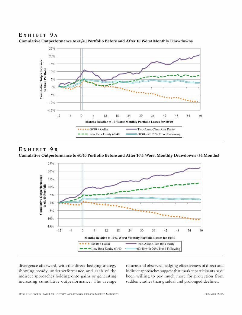
Exhibits 9A and 9B compare the performance of the direct and indirect approaches to 60/40 before and after the worst 60/40 monthly returns using an event study. In Exhibit 9A, we set the 10 worst 60/40 single

month drawdowns18 (or the 3% worst months) as t = 0, and returns are averaged across the 10 paths leading up to and after each drawdown. Exhibit 9B follows the same methodology, but using the 10% worst months (or 34 worst months). In both cases, we find relative outperformance for the direct hedge around t = 0 (the worstdrawdown composite), but noticeable subsequent

e x h i b i t 7Premium of 7.5% OTM Three-Month Put Option

e x h i b i t 8Cumulative Excess Return of Collar and Put Portfolios


divergence afterward, with the directhedging strategy showing steady underperformance and each of the indirect approaches holding onto gains or generating increasing cumulative outperformance. The average

returns and observed hedging effectiveness of direct and indirect approaches suggest that market participants have been willing to pay much more for protection from sudden crashes than gradual and prolonged declines.

e x h i b i t 9 ACumulative Outperformance to 60/40 Portfolio Before and After 10 Worst Monthly Drawdowns

e x h i b i t 9 bCumulative Outperformance to 60/40 Portfolio Before and After 10% Worst Monthly Drawdowns (34 Months)


constructed to be better behaved, with more consistent risk levels and, ideally, fewer and smaller tails. Compared with direct approaches to hedging portfolio tail risk, the indirect approaches described in this study have offered a more efficient way of working your tail off. Directly buying portfolio insurance through options, though riskreducing, does not lead to more efficient risk taking.

A p p e n d i x APUT STRATEGIES

Our analysis focused on collars, but a more direct method of tail hedging using options would be to buy puts. Here we compare the performance of an equity collarhedged 60/40 portfolio with an equity puthedged 60/40 portfolio. The parameters used for the putsonly hedge are identical to the put component of the 92.5–110 collar strategy described earlier.

As shown in Exhibit A1, the put portfolio was a more expensive way to hedge the portfolio than the collar, generating worse performance in each of the worst months for equities and over the worst equity drawdowns.

Real-world challenges. Both the direct and indirect approaches require expertise to implement efficiently. The indirect approaches are active strategies that involve risk estimation, portfolio rebalancing, use of derivatives (for risk parity and trend following) and the ability to hold short positions (for trend following). The direct approach, though viewed by some as a lessactive strategy, still imposes a number of implementation challenges. Investors must determine how much they are comfortable losing (and over what period) in order to size their hedge appropriately. It may also be difficult for investors to stick to an insurance program after years of negative performance. All of these add to the cost of an insurance program, even for investors with substantial experience in trading derivatives and, for institutions, the right oversight board.19 For both direct and indirect approaches, investors must also ensure they receive fair pricing, manage transaction costs, and understand and manage counterparty risk and documentation.

CONCLUSION

Economic theory and empirical evidence support the idea that investors should, over the long term, be compensated for bearing risk. Thus, any discussion of tail risk should rationally start from the premise that it’s something that contributes to a portfolio’s expected returns.20

In this article, we’ve demonstrated that several active strategies that are straightforward to implement in portfolios not only deliver superior longterm average returns but also outperform direct hedges in prolonged market drawdowns. Importantly for investors, these indirect hedging strategies can be combined, and a portfolio of them may offer investors a more robust way to mitigate their sensitivity to the worst drawdowns in equity markets. In contrast, we f ind direct hedging is costly and only delivers value when combined with the ability to time shortterm market crashes and the ability to unwind those hedges very shortly after those events. We question investors’ ability to do either of those.

Capital market risk includes tail risk. Though preparing for and embracing risk is one element of investing, a second element is to capture risk in the most efficient way possible. More efficient portfolios make it easier to bear risk if they can be

e x h i b i t A 1Standard Statistics of the Portfolios, 1985–2012


A p p e n d i x b

ROBUSTNESS CHECKS

There are many moving parts in optionbased hedging strategies, such as which strikes and maturities to use. In this section, we compare our hedging strategy with the S&P 500 95–110 Collar Index (CLL) published by the CBOE. The CLL index differs from our strategy in that it:

• Uses 5% OTM instead of 7.5% OTM puts.• Holds only the quarterly options (March/June/

September/December).• Rebalances if the strike of the new call is lower than

that of the standing put.

Exhibit B1 shows the scatter plots of the CLL Index monthly return versus the S&P 500 hedged with our 92.5110 Collar Index. Regressing our return onto the index returns shows an R2 of 0.93 with no significant alpha.

ENDNOTES

We thank Cliff Asness, Aaron Brown, Antti Ilmanen, Ronen Israel, John Liew, and Mark Stein for edits and comments.

1Although volatility is not a complete or comprehensive measure of risk, any reasonable definition of risk will show equities are two to three times as risky as bonds.

2Proxied by 60% S&P 500 and 40% Barclays U.S. Government Bonds Index. Though few investors individually hold this exact portfolio, anecdotal evidence suggests it’s a useful benchmark for the major risks the average investor faces.

3A putsonly strategy performed worse over the full sample, and a comparison of the two approaches is provided in Appendix A.

4The monthly returns of the two series in the period where we have overlapping data (1996–2004) are 0.97 correlated, with neither statistically significant nor economically meaningful alpha to the other. The use of two options series to build a longer time series ref lects the deeper liquidity and more prevalent use of S&P 100 options in the earlier part of the sample. S&P 100 data are from Commodity Systems Inc., and S&P 500 options data are from OptionMetrics.

5For returns using different combinations of maturities, strikes, and rebalancing rules, see Israelov and Nielsen [2013].

6Our methodology does not necessarily result in a cashless collar but the results for those strategies are analogous to those shown here. The performance of the S&P 500 95110 Collar Index (CLL) is consistent with the performance described above, but with even worse performance following the October 1987 crash, as the strategy rebalances when options become inthemoney. For more details, see Appendix B.

7There are related methods, such as minimumvolatility investing, and a range of defensive equity strategies, all of which seek to earn higher riskadjusted returns than capweighted market indexes, while realizing lower volatility.

8Black et al. [1972]; Fama and French [1992]; Baker et al. [2011]; and Frazzini and Pedersen [2014] for U.S., international, and acrossassetclass evidence.

9The starting universe used to build the lowbeta portfolio is approximately the Russell 3000.

10This is the average realized volatility of the 60/40 portfolio over the 1985–2012 period and comparable to longer periods, including 1903–2012.

11In practice, riskparity portfolios include many more asset classes, notably inf lationhedging assets such as commodities and inf lationlinked bonds. Given more assets leads to higher expected portfolio eff iciency, we would expect the twoassetclass riskparity example here to understate the benefits that a typical riskparity portfolio lends to tailrisk management. Further, many riskparity portfolios also incorporate measures of correlation in sizing positions, which we leave out of this analysis for the sake of simplicity. We find that using correlation estimates also improves risk–return tradeoffs, which lends a second degree of conservatism to our results. Finally, volatilitytargeted approaches often use shorterterm measures than the trailing 12month average volatility used here, which may further benefit returns during adverse markets. For further studies on riskparity portfolios, see Asness et al. [2012] and Asness et al. [2013].

12Commonly known as managedfutures strategies, or time series momentum.

e x h i b i t b 1CLL Index vs. 92.5–110 Collar Monthly Returns, 1985–2012


13In practice, trendfollowing strategies such as managed futures invest across multiple asset classes and regions. Twoasset trend following is suboptimal but investigated here for comparability to the 60/40 portfolio. For studies on multipleasset trend following, see Moskowitz et al. [2011] and Hurst et al. [2013].

14This allocation was chosen so that the correlations of this portfolio to 60/40 and of the directhedged portfolio to 60/40 are the same (0.96).

15Given an investor’s prior beliefs that tail events in one asset class (stocks) do not coincide with tail events in the others (in this case, only bonds), this result may be expected.

16Though we would argue that 90% of risk exposed to a single tail is scarier.

17Corresponding to the economic events listed in Exhibit 5.

18Expressed as standard deviations, the worst month, October 1987, is a –4.5 fullsample standard deviation event (–12.2% return), and the 10thworst month, January 2009, is a –2.12 standard deviation event (–5.51% return).

19Still, some investors might buy insurance for reasons other than reducing tail risk. For example, insurance can provide a cash buffer in times of market distress, potentially allowing investors to take advantage of fire sales and other market dislocations. However, depending on the magnitude and frequency of the dislocations (and the manager’s ability to identify them), this opportunistic approach still might not make up for the negative expected returns from buying insurance. Other investors might occasionally have a tactical view that insurance is conditionally cheap. However, this is simply market timing in another form, and this decision should be made (and sized) in the context of other tactical views in the portfolio. Finally, some investors might be forced into insurance strategies for board or plan governance reasons independent of tail risks, but related to risk tolerances.

20Bollerslev and Todorov [2011] suggest that compensation for rare events accounts for a large fraction of the average equity risk premium; Jiang and Kelly [2013] extend to long/short strategies and find that tail risk is a key driver of hedge fund returns in both the time series and the cross section; Xiong et al. [2014] find that tail risk is compensated with higher expected returns in both U.S. and nonU.S. equity mutual funds.

REFERENCES

Asness, C., A. Frazzini, and L.H. Pedersen. “Leverage Aversion and Risk Parity.” Financial Analysts Journal, Vol. 68, No. 1 (2012).

Asness, C., A. Ilmanen, and J. Liew. “Risk Parity LifeCycle Investing,” Working paper, AQR, 2013.

Baker, M., B. Bradley, and J. Wurgler. “Benchmarks as Limits to Arbitrage: Understanding the LowVolatility Anomaly.” Financial Analysts Journal, Vol. 67, No. 1 (2011).

Black, F., M.C. Jensen, and M.S. Scholes. “The Capital Asset Pricing Model: Some Empirical Tests.” In Studies in the Theory of Capital Markets, edited by M.C. Jensen. New York, NY: Praeger, 1972.

Bollerslev, T., and V. Todorov. “Tails, Fears and Risk Premia.” Journal of Finance, Vol. 66, No. 6 (2011).

Fama, E.F., and K.R. French. “The CrossSection of Expected Stock Returns.” Journal of Finance, Vol. 47, No. 2 (1992).

Frazzini, A., and L.H. Pedersen. “Betting Against Beta.” Journal of Financial Economics, 2014.

Hurst, B., Y.H. Ooi, and L.H. Pedersen. “Demystifying Managed Futures.” Journal of Investment Management, 2013.

Israelov, R., and L. Nielsen. “Design Choices in OptionsBased Insurance Strategies.” Working paper, AQR, 2013.

Jiang, H., and B. Kelly, “Tail Risk and Hedge Fund Returns.” Working paper, University of Chicago, 2013.

Moskowitz, T., Y.H. Ooi, and L.H. Pedersen. “Time Series Momentum.” Journal of Financial Economics, Vol. 104, No. 2 (2011).

Xiong, J., T. Idzorek, and R. Ibbotson. “Volatility versus Tail Risk: Which One Is Compensated in Equity Funds?” The Journal of Portfolio Management, 2014.

To order reprints of this article, please contact Dewey Palmieri at [email protected] or 212-224-3675.

the journal of - home | institutional investor 015 the journal of investing sample (in fact,...

Documents