the influence of sea currents on the behaviour of the swan ... · hidrodinâmica ambiental)...

A. F. Santos Ramos / Instituto Superior Técnico (2014)

1

The influence of sea currents on the behaviour of the SWAN model in the

Diogo Lopes area, Brazil

André Filipe Santos Ramos

[email protected]

Department of Civil Engineering, Arquitecture and Georesources, Instituto Superior Técnico, ULisboa, Av.

Rovisco Pais, 1049-001, Lisbon-Portugal

July 2014

Abstract : Over the past few years the Diogo Lopes region, located in the state of Rio Grande do Norte , Northeast

Brazil, has been the object of a number of interdisciplinary studies including the characterization of its wave

climate (Ângelo, 2012; Matos, 2013). The wave climate is characterized by a breeze regime. The alternation

between the sea and land breezes along this coastline posed a few difficulties to its correct modelling. In order to

overcome these difficulties, the SWAN model was used once again to simulate the wave propagation. This time a

larger domain and a different wind field, obtained in the meteorological station in Macau (RN), were employed.

Also, a current field was imposed to take into account wave-currents interaction. These currents were calculated

by the hydrodynamic model SISBAHIA, developed in the Federal University of Rio de Janeiro (UFRJ). The

offshore wave conditions were obtained from the deep-water wave model, Wavewatch III (Tolman, 2002). Field

data were obtained through de measurements of AWAC sensors for the time periods from the 11th to the 12th of

December 2010 and from the 20th to the 27th December 2010 in two distinct points inside the computational grid.

The analysis of the results was accomplished resorting to both graphical analysis and statistic characterization.

Key words: SWAN; Wave-Currents; Diogo Lopes; SISBAHIA; Wave Climate; Whitecapping.

1 INTRODUCTION

The Diogo Lopes area, located in the state of Rio Grande do Norte, Northeast Brazil (Figure 1.1), is characterized

by a tropical climate, which dominates the environment. In the study area there are minor estuaries of rivers and

lagoons that disembogue in the Atlantic. Due to its complexity, this area has been the focus of several

environmental studies and monitoring programs, which intend to contribute to the understanding of the coastal

processes and their evolution. In those studies Matos (2013), among others, have pointed out to the need of better

knowledge on waves, tides and winds, as well on the hydrodynamic circulation in the study area. In fact, the

complex bathymetry and tidal circulation make the wave propagation not a trivial exercise and the correct

estimation of the wave field here is of paramount importance for sediment dynamics, coastal morphodynamic


2

studies, and coastal engineering design. Furthermore, the wave climate in Diogo Lopes is mainly affected by the

alternation between the sea and land breezes. However, existing information regarding sea waves and their

propagation in this region are insufficient for any study of coastal engineering. To overcome this problem,

numerical models of wave propagation constitute a viable alternative for estimating the wave climate. In the

present study, the SWAN model, that stands for Simulating WAves Nearshore (Booij et al., 1999), was used to

simulate the sea state. This model estimates the characteristic parameters of the wave climate through the

directional spectrum. More specifically, the present dissertation follows the work developed by Ângelo (2012) and

Matos (2013) that applied the SWAN model with different wind and offshore conditions, comparing the numeric

simulations with measurements in situ in two distinct points (PT1 and PT2) for the time periods from the 11th to

the 12th of December 2010 and from the 20th to the 27th December 2010.

Figure 1.1 - Diogo Lopes location in the state of Rio Grande do Norte, Brazil. Adapted Google Maps.

The results obtained through these studies were quite satisfactory. However, some differences were noticed

between the calculated and the observed values of the mean period (Tm02). One of the major suggestions made

by the authors of these works, to improve the calculated values of the mean period, was to include a current field

in the SWAN model simulations. In fact, since the study area is located in an estuary zone, this wave-current

interaction becomes of major importance. With a current field is possible to consider the Doppler effect and

consequently it is expected that the calculated values of the mean wave period become closer to the real ones. The

present dissertation consisted in the application of the SWAN model in the Diogo Lopes area forced in the offshore

boundary and by a wind field. Moreover, the wave filed will be propagated in a current field within the SWAN

computational grid. The former was substantially extended in the seaward direction. The SWAN model is applied

to the time periods from the 11th to the 12th and from the 20th to the 27th of December 2010. The numeric results

are compared with the field measurements obtained in these same time periods.

2 THE SWAN MODEL

The SWAN model (Booij et al., 1999; SWAN Team, 2008) is a third generation spectral wave model designed to

simulate wave propagation in a large range of depths, including nearshore shallow waters. In order to operate this


3

model, the user has to define a computational grid, associated to a bathymetry grid. The model uses implicit

numerical schemes. The offshore boundary conditions result from the coupling with deep water oceanic scale

models like WAM or Wavewatch III.

The SWAN model is based on the spectral action balance equation. This equation may be formulated in spherical

coordinates for big scale computations or Cartesian coordinates for smaller applications. In the present dissertation,

the equation (2.1) was used in Cartesian coordinates .

𝜕𝑁(𝜎,𝜃;𝑥,𝑦,𝑡)

𝜕𝑡+

𝜕𝑐𝑔,𝑥𝑁(𝜎,𝜃;𝑥,𝑦,𝑡)

𝜕𝑥+

𝜕𝑐𝑔,𝑦𝑁(𝜎,𝜃;𝑥,𝑦,𝑡)

𝜕𝑦+

𝜕𝑐𝜃𝑁(𝜎,𝜃;𝑥,𝑦,𝑡)

𝜕𝜃+

𝜕𝑐𝜎𝑁(𝜎,𝜃;𝑥,𝑦,𝑡)

𝜕𝜎=

𝑆(𝜎,𝜃;𝑥,𝑦,𝑡)

𝜎 ( 2.1 )

This equation uses the action density 𝑁(𝑥, 𝑡, 𝜎, 𝜃) in space 𝑥 and time t, instead of the spectral energy density E,

since E is not conservative when propagating between waves and currents.

𝑁(𝜎, 𝜃) =𝐸 (𝜎,𝜃)

𝜎 ( 2.2 )

𝜎 represents the relative frequency and 𝜃 is the wave direction.

The left member of (2.1) represents the local variation and the cinematic component of the propagation in its

various dimensions. The right member represents the source and sinks terms. The second and third parcels, of the

left member, correspond to the wave propagation in the geographic space with propagation velocities 𝑐𝑔 ,𝑥 and 𝑐𝑔,𝑦

in 𝑥 and 𝑦 space, respectively. The fourth parcel includes in this equation the refraction induced by the depth

variation and trough the currents effect, with 𝑐𝜃 corresponding to the spectral space velocity, 𝜃 (wave direction).

Finally, the fifth parcel stands for the variation of the angular frequency due to variations of the depth and currents,

with 𝑐𝜎 corresponding to the propagation velocity in the relative frequency domain, 𝜎.

The left term of (2.1), 𝑆(𝜎, 𝜃), stands for the effects of generation by wind 𝑆𝑖𝑛(𝜎 ,𝜃), non-linear wave-wave

interactions 𝑆𝑛𝑙(𝜎, 𝜃) and dissipation 𝑆𝑑𝑖𝑠𝑠 (𝜎, 𝜃).

3 CASE STUDY – THE DIOGO LOPES ESTUARY, BRAZIL

3.1 The available data

As mentioned before, the present study had the objective of improving the application conditions of the SWAN

model in this region, taking into account its climate characteristics and also the available data. In particular, the

wind measurements were obtained at the Macau meteorological station at a 4 m height, the measurements of wave

height, period and direction were made through two acoustic wave and curren t meter sensors (AWAC). The location

of the sensors is represented in Figure 3.1. The wind field was considered constant in the whole domain, and was

measured with a temporal resolution of one hour in the mentioned periods. The offshore boundary conditions,

parameterized by the significant height Hs, peak period Tp and mean direction Dir, were obtained as the output of

the WAVEWATCH III deep water model in one point. This point corresponds to the Cartesian coordinates UTM

(787166.43 m, 9668067.83 m). The current field was obtained by the SISBAHIA model (Sistema de Base

Hidrodinâmica Ambiental) (Rosman, 2000), and uses the Large Eddy Simulation (LES) as the turbulence closure

model. The SISBAHIA model has been implemented and improved since 1987. This model is subdivided in

multiple modules. For further information referring to SISBAHIA see Rosman (2000).


4

Figure 3.1 – Location of the Domain, nested grids and measurement points.

3.2 The SWAN model application conditions

The definition of the main SWAN grid was conditioned by the available bathymetry data in the Diogo Lopes area.

The bathymetry used in the present dissertation is, essentially, the same used by Ângelo (2012) and Matos (2013).

However, the seaward boundary was positioned further way with two main objectives. The previous main grid

had a minor stretch that was located over medium shallow waters and this new one configures a domain totally

over deep waters. On the other hand, it was possible to make the boundary closer to the WWIII output point. The

SWAN grids properties can be consulted on Table 3.1.

The SWAN 40.72 version was used in this work. Diffraction, non-linear three and four wave interaction were some

of the physical phenomena considered. Concerning the bottom friction the semi-empiric JONSWAP expression

was adopted (Hasselmann et al., 1973). Depth induced breaking and whitecapping were also considered . The

former was parameterized according to the van der Westhuysen et al. (2007) formulation for this phenomenon.

The discretization of the directional spectra was made with 23 frequency intervals, between 0.04 Hz and 1.0 Hz,

with a logarithmic distribution. Two operation modes – stationary and non-stationary were considered. Changes

in the bottom friction coefficient to use in the JONSWAP formulation were experimented. However, simulations

with a current field was the main test objective. In Ângelo (2012) a large number of bottom friction coefficients

were tested. In the present work, this choice was narrowed to a couple of values. One of those values is the default

value defined by the SWAN model for wind sea (c=0.067 m2s -3) and the other was fixed in c=0.1 m2s -3.


5

Summarizing, there were made 16 numerical simulations – 8 for each period of measurements. The entire bottom

friction coefficient – currents conditions possible combinations were tested, as illustrated in Tables 3.2 and 3.3.

Table 3.1 - SWAN grids properties.

Grids Origin (x, y) (m) Dimensions(km) ∆x(m) ∆y(m)

Main Grid (709869, 943260) 99.5x107.5 1000 1000

Nested grid (750000, 9440000) 50x20 500 250

Inner grid (Nested1) (765000, 9440000) 30x10 100 50

Table 3.2 - Numeric simulations conditions for the period from de 11 th to the 12th of December 2010.

Mode Bottom Friction Coefficient (m2s -3) Currents’ conditions

Simulation 1

Stationary

0.1 Yes

Simulation 2 0.1 No

Simulation 3 0.067 Yes

Simulation 4 0.067 No

Simulation 5

Non-stationary

0.1 Yes

Simulation 6 0.1 No



Table 3.3 - Numeric simulations conditions for the period from the 20 th to the 27th of December 2010.

Mode Bottom Friction Coefficient (m2s -3) Currents’ conditions

Simulation 9

Stationary

0.1 Yes




Simulation 13

Non-stationary

0.1 Yes




4 RESULTS: COMPARISON AND ANALYSIS

For all the graphics presented in this section, the same nomenclature was used in the definition of the numeric al

simulations, as follows:

“Corr” – Simulation which took into account a current field;

“SemCorr” – Simulation which did not take into account a current field;


6

“01” – Use of the 0.1 m2s -3 value for the bottom friction coefficient;

“0067” – Use of the 0.067 m2s -3 value for the bottom friction coefficient.

“Medições” – Measurements obtained in situ.

4.1 The 11th to 12th of December 2010 period

In this period, and in what concerns the significant wave height, the introduction of a current field did not induce

major changes in this parameter. On the other hand, the bottom friction coefficient has an important role on the

accuracy of the significant height´s behaviour. As expected, the increase of the bottom friction is accompanied by

a decrease of the calculated significant height. It is possible to verify this in Figure 4.1, for PT1, and Figure 4.2

for PT2. In this period, the best-obtained values are accomplished when applying a c=0.067 m2s -3 bottom

coefficient value with a current field and in stationary mode.

Figure 4.1 - Simulations 3 and 4. Significant height for PT1 from the 11 th to the 12th December 2010. Stationary

mode. c=0.067 m2s-3.

Figure 4.2 - Simulations 3 and 4. Significant height for PT1 from the 11 th to the 12th December 2010. Stationary

mode. c=0.067 m2s-3.

Focusing now on the mean wave period, it is verified, in general, that it is possible to achieve improvements when

considering a current field (Figures 4.3 and 4.4). However, the bottom friction coefficient ´s values have also an

important influence in the Tm02 calculated values. The increase of the bottom friction coefficient´s values

generates smaller values of the calculated Tm02.

0,00

0,20

0,40

0,60

0,80

1,00

1,20

1,40

11-12-10 12:00 12-12-10 0:00 12-12-10 12:00 13-12-10 0:00Sig

nif

ica

nt

He

igh

t -

Hs

(m)

Date and Time

Significant height PT1

Medições_PT1

SWAN_Corr_0067

SWAN_SemCorr_0067

0,00

0,50

1,00

1,50

2,00

11-12-10 12:00 12-12-10 0:00 12-12-10 12:00 13-12-10 0:00

Sig

nif

ica

nt

hig

ht

-H

s (m

)

Date and Time

Significant height PT2Medições PT2

SWAN_Corr_0067

SWAN_SemCorr_0067


7

Figure 4.3 - Simulations 3 and 4. Mean period for PT1 from the 11th to the 12th December 2010. Stationary

mode. c=0.067 m2s-3.

Figure 4.4 - Simulations 3 and 4. Mean period for PT2 from the 11th to the 12th December 2010. Stationary

mode. c=0.067 m2s-3.

For a better analysis the statistical parameters for simulations 3 and 4 are presented in Table 4.1.

Table 4.1 - Statistic parameters for the period from the 11 th to the 12th December 2010 in stationary mode.

(c=0.067m2s-3)

Sationary mode

c(m2s

-3) Currents’ conditions PT1 PT2

0.067

With currents

(Simulation 3)

RMSE RMSE

Hs(m) Tm0,2(s) Dir(º) Hs(m) Tm0,2(s) Dir(º)

0.127 0.732 23.097 0.204 0.961 67.044

SI SI Hs Tm0,2 Dir Hs Tm0,2 Dir

0.134 0.196 ___ 0.177 0.211 ___

ME ME Hs(m) Tm0,2(s) Dir(º) Hs(m) Tm0,2(s) Dir(º)

-0.021 0.616 -21.439 -0.226 -0.584 -15.468

Without currents (Simulation 4)

RMSE RMSE

Hs(m) Tm0,2(s) Dir Hs(m) Tm0,2(s) Dir

0.130 1.164 25.209 0.228 0.965 66.509

SI SI

Hs Tm0,2 Dir Hs Tm0,2 Dir

0.138 0.311 ___ 0.199 0.212 ___

ME ME

Hs Tm0,2 Dir Hs Tm0,2 Dir

-0.002 1.046 -24.163 -0.280 -0.645 -14.596

0

1

2

3

4

5

6

7

11-12-10 12:00 12-12-10 0:00 12-12-10 12:00 13-12-10 0:00

Me

an

pe

rio

d -

Tm

0,2

(s)

Date and Time

Mean period (Tm02) PT1

Medições_PT1

SWAN_Corr_0067

SWAN_SemCorr_0067

0

1

2

3

4

5

6

7

11-12-10 12:00 12-12-10 0:00 12-12-10 12:00 13-12-10 0:00

Me

an

pe

rio

d -

Tm

0,2

(s)

Date and Time

Período Médio (Tm02) PT2

Medições PT2

SWAN_Corr_0067

SWAN_SemCorr_0067


8

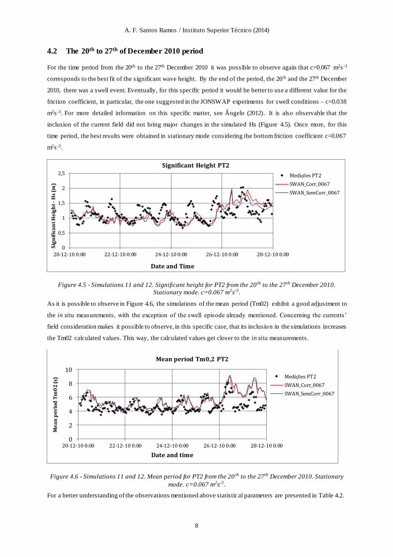
4.2 The 20th to 27th of December 2010 period

For the time period from the 20th to the 27th December 2010 it was possible to observe again that c=0.067 m2s -3

corresponds to the best fit of the significant wave height. By the end of the period, the 26th and the 27th December

2010, there was a swell event. Eventually, for this specific period it would be better to use a different value for the

friction coefficient, in particular, the one suggested in the JONSWAP experiments for swell conditions – c=0.038

m2s -3. For more detailed information on this specific matter, see Ângelo (2012). It is also observable that the

inclusion of the current field did not bring major changes in the simulated Hs (Figure 4.5). Once more, for this

time period, the best results were obtained in stationary mode considering the bottom friction coefficient c=0.067

m2s -3.

Figure 4.5 - Simulations 11 and 12. Significant height for PT2 from the 20 th to the 27th December 2010.

Stationary mode. c=0.067 m2s-3.

As it is possible to observe in Figure 4.6, the simulations of the mean period (Tm02) exhibit a good adjustment to

the in situ measurements, with the exception of the swell episode already mentioned. Concerning the currents’

field consideration makes it possible to observe, in this specific case, that its inclusion in the simulations increases

the Tm02 calculated values. This way, the calculated values get closer to the in situ measurements.

Figure 4.6 - Simulations 11 and 12. Mean period for PT2 from the 20 th to the 27th December 2010. Stationary

mode. c=0.067 m2s-3.

For a better understanding of the observations mentioned above statistical parameters are presented in Table 4.2.

0

0,5

1

1,5

2

2,5

20-12-10 0:00 22-12-10 0:00 24-12-10 0:00 26-12-10 0:00 28-12-10 0:00

Sig

nif

ica

nt

He

igh

t-

Hs

(m)

Date and Time

Significant Height PT2

Medições PT2

SWAN_Corr_0067

SWAN_SemCorr_0067

0

2

4

6

8

10

20-12-10 0:00 22-12-10 0:00 24-12-10 0:00 26-12-10 0:00 28-12-10 0:00

Me

an

pe

rio

d T

m0

2 (

s)

Date and time

Mean period Tm0,2 PT2

Medições PT2

SWAN_Corr_0067

SWAN_SemCorr_0067


9

Table 4.2 - Statistic parameters for the period from the 20 th to the 27th December 2010 in stationary mode.

(c=0.067m2s-3)

c(m2s

-3) Stationary Mode

0.067

With Currents

(Simulation 11)

RMSE

Hs(m) Tm0,2(s) Dir(º)

0.263 1.228 128.962

SI

Hs Tm0,2 Dir

0.227 0.261 ___

ME Hs(m) Tm0,2(s) Dir(º)

0.002 0.840 -47.137

Without Currents (Simulation 12)

RMSE Hs(m) Tm0,2(s) Dir(º)

0.252 1.297 120.801

SI

Hs Tm0,2 Dir

0.218 0.276 ___

ME

Hs(m) Tm0,2(s) Dir(º)

-0.074 0.888 -58.284

5 CONCLUDING REMARKS

This dissertation had as main objective the introduction of currents on the SWAN model ´simulations in the Diogo

Lopes area, Brazil. The present work follows the previous studies by Ângelo (2012) and Matos (2013) with the

aim of improving the calculated results with a special emphasis on the mean wave periods.

In what concerns the significant height the bottom friction coefficient is the key factor influencing the calculated

values. Meanwhile, is possible to verify that better results are obtained when the bottom friction coefficient

suggested by Bouws & Komen (1984) for wind sea is applied (c = 0.067 m2s -3). As for the impact of the currents

conditions in this wave parameter, is possible to say that its changes have almost no influence on the calculated

significant wave heights. The stationary runs become more cost-effective in terms of the relation between the

calculated values and computation time, since the non-stationary runs need more time to be accomplished and do

not lead to better results.

Focusing on the mean periods and comparing with previous works in this very geographic location, we can observe

a reasonable improvement on the obtained results, which previously were, in general, underestimated.

The analysis of the statistical parameters shows that improvements are achieved when a current field is present.

The bottom friction coefficient which results on the better-calculated values is c=0.067 m2s -3. However, a careful

observation should be made concerning the 11th to the 12th of December period, where is possible to compare the

results from two distinct geographic points inside de computational domain. The numerical simulations obtained

for the c=0.067 m2s -3 bottom friction coefficient, with the currents’ field consideration were better for PT2

comparing with PT1.

6 REFERENCES

Ângelo, J. C. F. (2012). Aplicação do modelo SWAN na caracterização da agitação marítima na zona adjacente

ao estuário de Diogo Lopes , Brasil. Instituto Superior Técnico.


10

Booij, N., Ris, R., & Holthuijsen, L. (1999). A third-generation wave model for coastal regions. I- Model description and validation. Journal of Geophysical Research , 104(C4), 7649–7666.

Bouws, E., & Komen, G. J. (1984). On the balance between growth and dissipation in a extreme, depth -limited wind-sea in the southern North Sea. Journal of Physical Oceanography, 13(9), 1653–1658.

Hasselmann, K., Barnett, T. P., Bouws, E., Carlson, H., Cartwright, D. E., Enke, K., Ewing, J. A., Gienapp, H.,

Hasselmann, D. E., Kurseman, P., Meerburg, A., Müller, P., Olbers, D. J., Richter, K., Sell, W., Walden,

H. (1973). Measurements of wind-wave growth and swell decay during the Joint North Sea Wave Project (JONSWAP) (Vol. 8). Deutches Hydrographiches Institut.

Matos, M. de F. A. (2013). Modelagem do clima de ondas e seus efeitos sobre as feições morfológicas costeiras

no Litoral Setentrional do Rio Grande do Norte. Universidade Federal do Rio Grande do Norte.

Rosman, P. C. C. (2000). Referência Técnica do SisBaHiA – SISTEMA BASE DE HIDRODINÂMICA

AMBIENTAL. Programa COPPE: Engenharia Oceânica, Área de Engenharia Costeira e Oceanográfica, Rio de Janeiro, Brasil.

SWAN Team. (2008). TECHNICAL DOCUMENTATION SWAN Cycle III version 40.51 .

Tolman, H. L. (2002). User manual and system documentation of WAVEWATCH-III version 2.22 (p. 133 pp.).

U S Army Corps Of Engineers. (2002). Coastal Engineering Manual. Coastal Engineering Manual.

Van der Westhuysen, A. J., Zijlema, M., & Battjes, J. a. (2007). Nonlinear saturation-based whitecapping

dissipation in SWAN for deep and shallow water. Coastal Engineering, 54(2), 151–170.

7 ACKNWOLEDGEMENTS

To the Geoprocessing Laboratory from the Geology Department at Federal University of Rio Grande do Norte,

for the bathymetry, wave parameters and tide data, and also to the Oceanic Engineering Program from

COPPE/UFRJ for the SISBAHIA model operation.

the influence of sea currents on the behaviour of the swan ... · hidrodinâmica ambiental)...

Documents