the impact of tariff trade barriers on the operating

The Impact of Tariff Trade Barriers on the Operating Performance of U.S. Firms: The Role of Supply Structure and ComplexityDi FanHong Kong Polytechnic University - Institute of Textiles and Clothing

Yi ZhouMonash University - Department of Management

Chris LoBusiness Division, Institute of Textiles and Clothing, Hong Kong Polytechnic University

Andy YeungHong Kong Polytechnic University - Department of Logistics and Maritime Studies

Christopher S. TangUniversity of California, Los Angeles (UCLA) - Decisions, Operations, and Technology Management (DOTM) Area

1

The Impact of Tariff Trade Barriers on the Operating Performance of U.S. Firms: The

Role of Supply Structure and Complexity

Abstract

Multinational corporations (MNCs) have benefited tremendously from free trade in the

past few decades in the form of cost reductions, resource advantages, and market expansion.

However, the dynamism of international relations and a global recession have rekindled the debate

over frictionless trade. In this study, we examine how trade friction, created by tariff trade barriers,

affects the operational performance of domestic firms. We also investigate how different supply

chain characteristics and strategies can moderate the impact of such trade friction.

Motivated by the 2018 U.S.-China trade war, we conducted a difference-in-difference

analysis to examine the impact of trade tariffs on various firm performance indicators of U.S. firms.

We find that U.S. firms with direct supply chain partners (i.e., first-tier suppliers) in China have

worse performance in terms of inventory (days of supply) and profitability (ROA). We further

show that the negative impact on firms’ profitability is more severe when firms have a lower degree

of vertical integration and when firms have a higher degree of horizonal, spatial, and cooperative

supply base complexity. We discuss the implications for international operations management,

supply chain networks, and supply risk management, and provide suggestions to supply chain

practitioners and trade policy makers.

Keywords: Supply chain management, international, trade war, policy, difference-in-difference

2

Introduction

Since the 1980s, various favorable trade agreements established by various governments

have enticed many multinational corporations (MNCs) to offshore their operations to Asia,

creating complex global supply chains for industrial and consumer products. In the context of

stable, open trade, and a low-trade barrier global environment, research shows that, through these

cross-border transactions, firms can reduce cost and develop knowledge (Pitelis & Teece, 2010),

and improve efficiency of physical resources and increase business opportunities (Teece, 1986).

But there is also the flip side of global sourcing. Transaction costs economics (TCE) suggests

that global sourcing increases transaction and coordination costs that MNCs need to bear (Lampel

& Giachetti, 2013); these costs can be significant (Grover & Malhotra, 2003). Also, complex

global supply chains can make a firm vulnerable to dynamic changes in trade policies. The recent

emerged nationalism has triggered governments to impose new trade restrictions to de-globalize

(Witt, 2019). These new restrictions create major supply chain disruptions (Kouvelis et al., 2011),

forcing firms to rethink their global operational strategies (Charpin et al., 2020; Darby et al., 2020).

While researchers have examined various aspects of supply chain risks (e.g., Kleindorfer & Saad,

2005; Tang & Tomlin, 2008), empirical research investigating the impact of geopolitical tensions

and trade conflicts on firms’ operational performance remains nascent (Charpin et al., 2020).

In this paper, we examine the impact of trade tariffs on firms’ performance by using the

recent U.S.-China trade war declared by former President Trump as the backdrop. Since 2018,

over 1,300 categories and $50 billion of products imported from China were affected in the first

wave of 25% tariff increases (Office of the United States Trade Representative, 2018). Later on,

the scope was increased to $300 billion over 3,805 categories. To retaliate, China imposed tariff

increases for $75 billion of U.S. products.

3

The intent of increasing import tariffs was to reduce the trade deficit between the United

States and China, but U.S. firms have major concerns. The American Chamber of Commerce

found that 42% of its members experienced higher production costs, and over 50% of its members

believed that their product sales would decline (Bray, 2019). Huang et al. (2019) found a negative

stock market reaction toward higher import tariffs for firms importing from China. These

observations prompted us to examine our first research question (RQ1): How would the U.S.-China

trade war affect the operating performance of the U.S. firms sourcing from China? We measure

the operating performance in terms of inventory (days of supply) (Wiengarten et al., 2017; Darby

et al., 2020) and profitability (ROA) (Swift et al., 2019).

Grover & Malhotra (2003) conceptualize transaction cost as the sum of transaction risk

and coordination cost. Supply diversification is a major source of coordination cost in supply chain

management. The use of supply diversification as a risk mitigation strategy is controversial. On

the one hand, diversification can increase supply flexibility: alternative supply sources are

available when failures happen to a supply source (Hendricks et al., 2009; Tang & Tomblin, 2008).

On the other hand, diversification can also increase coordination difficulties and reduce

responsiveness to cope with uncertainty (Choi & Krause, 2006). This view is in line with the fact

that Japanese firms have significantly reduced their supply network complexity after the disruption

caused by the 2011 earthquake in eastern Japan (Son et al., 2021). We therefore also examine the

extent to which a firm’s degree of vertical integration (Hendricks et al., 2009; Steven et al., 2014)

and supply base complexity (Dong et al., 2020; Lu & Shang, 2017) would moderate or accentuate

the impact of the increased trade tariffs on a firm’s performance. Specifically, we examine our

second research question (RQ2): How would a U.S. firm’s supply structure and complexity affect

its capability in responding to the trade war?

4

To examine our research questions, we conducted a quasi-natural experiment to understand

the treatment effect of the U.S.-China trade war on U.S. firms’ operating performance. By focusing

on U.S. industries that are affected by the tariffs imposed in 2018, we compared the performance

changes for those sample firms with direct suppliers from China against those of control firms with

no direct suppliers in China. We used secondary data collected from COMPUSTAT (financial

data), Bloomberg’s SPLC, and the FactSet Reverse and COMPUSTAT Segment (supply chain

relationship data) databases, and adopted the propensity score matching (PSM) technique to

develop the matched pairs. The matching procedures ensure that the sample and control firms are

highly similar in terms of firm properties and supply network characteristics (e.g., second-tier

suppliers).

Our difference-in-difference (DID) regression analysis reveals that the sample firms suffer

from a more serious loss in operating efficiency (inventory – days of supply) and profitability

(ROA) than the comparable control firms. We further show that the negative impact on firms’

profitability is more severe for firms with a lower degree of vertical integration, and for firms with

a higher degree of horizonal, spatial, and cooperative supply base complexity (Choi & Krause,

2006; Dong et al., 2020). Overall, we find that supply base complexity exacerbates the negative

impact of the U.S.-China trade war. We also discuss the implications of our results in the context

of international operations management, supply chain networks, and supply risk management, and

provide suggestions to supply chain practitioners and trade policy makers.

5

Literature Review

Transaction Cost Economics (TCE) and Global Sourcing

TCE conceptualizes a firm’s “make or buy” decisions: low transaction cost is a key driver

for a firm’s outsourcing (or “buy”) decision (Coase, 1937). Relative to the century before, the

international transaction costs in the first decade of the 21st century were much lower owing to

technological advancement (Müller & Seuring, 2007) and stable trade (Oh et al., 2011). Besides

transaction costs, the pursuit of competitive advantage was another reason for global sourcing

(Kotabe & Murray, 2004). Global sourcing helps firms to differentiate products by exploiting

unique resources (Teece, 1986); increase firms’ bargaining power over their suppliers (Lampel &

Giachetti, 2013); and reduce costs (Jiang et al., 2007; Lampel & Giachetti, 2013).

TCE also highlights the challenges of global sourcing from the perspective of transaction

risk and coordination costs (Clemons et al., 1993; Grover & Malhotra, 2003). Transaction risk

causes disturbances to the global supply chain (Williamson, 2008) and affects operational

continuity and efficiency (Grover & Malhotra, 2003). Coordination costs are associated with

efforts to facilitate information exchanges, production rationalization, and process standardization

(Clemons et al., 1993; Lampel & Giachetti, 2013). Using the TCE framework, OM scholars have

developed two streams of literature (supply chain risk management and supply base complexity),

which we describe next.

Political Tension and Supply Chain Risk

Supply chain risks are defined as “the likelihood and impact of unexpected macro or micro

level events or conditions that adversely influence any part of a supply chain leading to operational,

tactical, or strategic level failures or irregularities” (Ho et al., 2015). The adverse influence

6

includes increased operational costs and reduced competitive advantages (Kwak et al., 2018; Tang,

2006). Global supply chains are more risky than domestic ones as the former involve more cross-

regional links that are prone to disruptions caused by macroeconomic and political changes (Manuj

& Mentzer, 2008). Thus, managing global supply chain risks requires cross-country coordination

and collaboration to ensure operational continuity and firm efficiency (Tang, 2006).

The supply chain risk literature focused on risk identification, assessment, mitigation, and

control at both macro- and micro-level types is vast (Ho et al., 2015). Most OM researchers

examined the impact of natural disasters: Hendricks et al. (2020) examined market reactions to the

supply chain disruptions caused by the 2011 Great East Japan Earthquake; and Shen et al. (2020)

investigated the impact of the Covid-19 pandemic on firm performance. Compared with

investigations of natural disasters, the research that examines the impact of man-made crisis (e.g.,

trade wars) on a firm’s performance is nascent (Darby et al., 2020). Charpin et al. (2020) find that

the foreign subunits of MNCs need to earn legitimacy to mitigate political uncertainty and risk. In

the Brexit context, Hendry et al. (2019), Roscoe et al. (2020), and Moradlou et al. (2021) find that

geopolitical tensions cause significant supply chain disruptions, entailing resilient and robust

supply chain designs. These qualitative studies provide valuable information, yet empirical

investigations are scarce (Charpin et al., 2020). Hence, our study fills a research gap by examining

the impact of the US-China trade war.

Supply Base Complexity

While firms have little control over political tensions and trade wars, they can mitigate

these risks through supply base diversification (e.g., Robinson, 2020; Schmitt et al., 2015; Shih,

2020; Tomlin & Wang, 2011). The merits of supply base diversification are illustrated by Nokia’s

7

multiple-sourcing strategy. By increasing the firm’s supply flexibility, supply base diversification

alleviated the disruption caused by fire in the Philips semiconductor factory in 2000 (Tang, 2006).

Choi & Krause (2006) argue that diversifying the supply base can lead to “supply base

complexity” in three dimensions: (1) multiplicity—the number of suppliers, (2) diversity—the

differentiations among the suppliers, and (3) interrelatedness—the interrelationship among

suppliers (Dong et al., 2020; Lu & Shang, 2017; Sharma et al., 2020). The complexity can increase

transactional uncertainty in the supply chain, requiring extra coordination efforts (Bode & Wagner,

2015). Research shows that supply base complexity hinders a firm’s use of its supply base’s R&D

development (Dong et al., 2020). It also creates delivery delays (Milgate, 2001; Vachon & Klassen,

2002), production disruptions (Bozarth et al., 2009), and quality problems (Steven et al., 2014).

Supply base complexity creates major difficulties for a firm to manage materials and information

flows (Brandon-Jones et al., 2015) and to coordinate among suppliers (e.g., Giri & Sarker, 2017;

Qi et al., 2004; Tang, 2006; Xiao et al., 2007). Hence, a firm with a higher supply base complexity

may be less resilient (Choi & Krause, 2006). Hendricks et al. (2009) find that firms with a higher

geographical diversification suffer a higher market value loss from supply disruptions. These

findings inspired us to establish a hypothesis suggesting that firms with higher supply base

complexity are likely to suffer more due to the increased trade tariffs.

Trade War

The U.S.-China trade war has prompted economists to examine its impact: Li et al. (2018)

estimated that the GDP and manufacturing employment for the world will be negatively affected;

Itakura (2020) estimated that the GDP of China and the United States will be reduced by 1.41%

and 1.35%, respectively; and Mao and Görg (2020) estimated that the EU, Canada, and Mexico

8

will face a burden of up to $1 billion. In the finance research literature, Burggraf et al. (2020)

found that tweets related to the U.S.-China trade war reduced the S&P 500’s returns and increased

market volatility. Huang et al. (2019) showed that U.S. firms with more supply and market

connections with China suffer from a stronger negative market reaction to the trade war.

Not much is known about the impact of increased trade tariffs associated with the U.S.-

China trade war on the firms’ operational performance (Plehn et al., 2010). Most OM analytical

models focus on examining how trade barriers affect a firm’s global procurement strategy (Wang

et al., 2011) and supply chain design (Hsu & Zhu, 2011). Lu and Van Mieghem (2009) and Dong

and Kouvelis (2020) found that import tariffs can make a firm reconfigure its global supply chain

network. Grossman and Helpman (2020) found that import tariffs can lead to the renegotiation of

buyer-supplier dyads or a buyer’s search for new suppliers. Nagurney et al. (2019) revealed that,

while some firms may benefit from trade barriers, the consumer welfare may be compromised.

Using data from the Korean automobile industry, Choi et al. (2012) found that import tariffs can

affect a firm’s postponement strategy. He et al. (2019) found that trade barriers can increase the

global and local environmental costs of agricultural production. By conducting in-depth

interviews, Roscoe et al. (2020) explored how firms implemented different strategies in response

to supply chain disruptions caused by Brexit. The above OM literature has provided grounds for

us to develop our hypotheses to explore how the increased trade tariffs affect firm performance.

9

Hypothesis Development

Trade Tariffs and the Performance of U.S. Firms Sourcing from China

Trade tariffs have been viewed as a supply chain disruptor (e.g., Grossman & Helpman,

2020; Handfield et al., 2020; Roscoe et al., 2020) that can affect a firm’s inventory performance

(days of supply) negatively. The increased import tariffs increase the costs of transacting with

Chinese suppliers (Roscoe et al., 2020). While U.S. firms can source beyond China, it is time-

consuming and costly (Burnson, 2019). Also, the increased tariffs created incentives for firms to

stock up before the increased tariffs took effect (Darby et al., 2020; Wu, 2018), piling up inventory

in warehouses throughout the United States in 2018 (Naidu & Baertlein, 2018).

Because the import tariffs have a direct impact on the trade operations between two

countries (the United States and China), our modeling framework is based on the general

equilibrium models of Tintelnot et al. (2018) and Huang et al. (2019) that involve one domestic

country and one foreign country. Specifically, in our study, our sample firms are U.S. firms with

direct first-tier suppliers in China, and the trade tariffs will affect these firms directly (Huang et

al., 2019). In contrast, as a benchmark, our control firms are U.S. firms with no direct suppliers in

China. Because tariff increases are less likely to affect inventory for our control firms, we propose

the following:

H1: The tariff increases associated with the U.S.-China trade war will increase the

inventory (days of supply) for U.S. firms with direct suppliers from China.

OM researchers have examined the role of tariffs from the cost perspective (e.g., Choi et

al., 2012; Wang et al., 2011) and the sales performance perspective (Dong & Kouvelis, 2020).

From the cost perspective, our sample firms will incur higher purchasing costs than our control

10

firms. A report from Moody’s revealed that U.S. importers absorbed 90% of the additional costs

resulting from the tariff levies (Lee, 2021). In the event that the sample firms hold more inventory

(due to advance purchases), these firms bear additional inventory holding, goods-in-transit, and

transportation costs. Therefore, the overall cost efficiency would be negatively affected. Our

argument was echoed by a survey of over 200,000 firms, which indicates that 40% of U.S. firms

reported that the trade war had increased their operating costs (Sim, 2020).

Some sample firms might choose to transfer the increased cost to their downstream

customers by increasing the product prices, but such a strategy would reduce sales. For example,

data show that a 20% tariff imposed by the U.S. government on foreign washing machines drove

U.S. washing machine prices up by 13%, while reducing demand by 3% (Tankersley, 2019). On

the other hand, our control firms with no direct connection to Chinese firms are much less affected

by the tariffs. Therefore, our sample firms with direct suppliers from China are likely to bear

additional costs, leading to lower profitability (ROA). Thus, we propose the following hypothesis:

H2: The tariff increases associated with the U.S.–China trade war will decrease the

ROA for U.S. firms with direct suppliers from China.

The Role of Supply Structure and Complexity

In addition to the direct impact of trade tariff increases on inventory and ROA as stated in

hypotheses H1 and H2, we investigate to what extent this impact is affected by a firm’s degree of

vertical integration. This exploration is based on Tang’s (2006) argument that supply chain risk

management requires extraordinary coordination efforts among the supply chain partners and Choi

& Krause’s (2006) suggestion that a complex supply structures reduce firms’ responsiveness in

coping with supply disruption. More broadly, our exploration fits in the two components of

11

transaction costs, namely transaction risk (i.e., the operational uncertainty due to the trade war)

and coordination costs (supply complexity). Specifically, we first examine the role of firm’s make

or buy structure (Steven et al., 2014) and the three dimensions of supply base complexity, namely

multiplicity, diversity, and interrelatedness (Choi & Krause, 2006; Dong et al., 2020).

In general, firms with a higher degree of vertical integration bear lower transaction costs

(Mahoney, 1992), and face a lesser impact should a trade war break out. However, firms with a

low degree of vertical integration can focus on core competency and exploit low-cost production

opportunities (Stevenson, 2018). However, as these firms outsource their operational tasks, they

have less control over their supplies (Hendricks et al., 2009), more vulnerability to disruptions

(Kleindorfer & Saad, 2005; Hendricks et al., 2009), more supply chain complexity, and higher

coordination costs (Steven et al., 2014). Therefore, we argue that the negative impact of the trade

war will be more severe for firms with a low degree of vertical integration:

H3: The negative impact of tariff increases on U.S. firm performance is more severe

for firms with a lower degree of vertical integration.

We also examine the extent to which the trade war’s impact is affected by a firm’s

horizontal (supply base) complexity (measured in terms of the number of suppliers) (Choi &

Krause, 2006). Firms with a lower degree of horizontal complexity can foster close, trusting

relationships (Heese, 2015); information sharing, collaborative planning, forecasting, and

replenishment (Hollman et al., 2015; Hsu et al., 2008); closer coordination; and more resilience to

disruptions (Treleven & Schweikhart, 1988). In contrast, research suggests that a large supply base

can reduce supplier responsiveness, hindering a firm’s ability to coordinate supply resources in

case of supply chain disruptions (Choi & Krause, 2006). Therefore, the negative impact of the

12

trade war will be more severe for firms with a higher degree of horizontal complexity. We postulate

the following:

H4: The negative impact of tariff increases on U.S. firms’ performance is more severe

for firms with a higher degree of horizontal (supply base) complexity.

In addition to horizontal complexity, firms have different degrees of spatial (supply base)

diversity. A spatially diversified supply base can increase a firm’s sourcing flexibility: it can shift

its supply to a different sourcing location to cope with supply chain disruptions and uncertainties

caused by the trade war. However, firms with a higher degree of spatial complexity find it difficult

to maintain close relationships and coordinate with suppliers (Choi & Krause, 2006) due to

different management styles, cultures, and operational practices of suppliers in different locations

(Dong et al., 2020; Sousa & Bradley, 2008). Consequently, the negative impact of the trade war

will be more severe for firms with a higher degree of spatial complexity. We thus postulate the

following:

H5: The impact of tariff increases on U.S. firms’ performance is more negative when

the firms have a higher spatial (supply base) complexity.

Besides supply complexity (degree of horizontal and spatial complexity), the relationships

among suppliers can create cooperative complexity (Lu & Shang, 2017). When suppliers are

substitutes (e.g., backup suppliers), supplier dependency is weak and suppliers operate

independently. Hence, the focal firm can act as a bridge controlling the information flow and thus

enjoy a more powerful status when interdependency among suppliers is absent or weak (Dong et

al., 2020).

13

When suppliers are complements (e.g., the output of one supplier will be used as input for

the other supplier), their operations are interdependent; disruption that occurs at one supplier can

affect the operations for the other supplier. Hence, when suppliers are complements, material,

information, and financial flow exchanges among suppliers will take place, leading to a supplier-

supplier relationship embedded in a buyer-supplier-supplier triad (Wu & Choi, 2005; Wu et al.,

2010). In this case, when interdependency among suppliers is present and strong, the focal firm

has little information advantage over suppliers, especially when the relationships across suppliers

are beyond the purview of the firm (Choi & Krause, 2006) and not so visible (Lu & Shang, 2017).

When dealing with a disruption in this environment, the focal firm would incur extra cost to

develop intersupplier cooperation and coordination. We thus postulate the following:

H6: The impact of tariff increases on U.S. firms’ performance is more negative when

the firms have a greater cooperative (supply base) complexity.

Figure 1 shows the theoretical framework of this study.

14

Figure 1. Theoretical framework

U.S.-China

Trade War

Inventory days

of supply of

U.S. firms

Profitability

(ROA) of U.S.

firms

H1:+, prolongs

H2:-, reduces

Vertical

integration

Horizontal

supply base

complexity

Spatial supply

base complexity

Cooperative

supply base

complexity

H3: Mitigate H4: Worsen

Political risk/trade war

Supply Chain

coordination complexity

H5: Worsen H6: Worsen

15

Method

Data Collection

Company lists

We sampled U.S. firms in industries affected by the U.S.-China trade war tariff increases

as follows. The Office of the United States Trade Representative (USTR) announced three trade

action industry lists in 2018 and one in 2019. We used the three lists announced in 2018 because

the impact of tariff increase can be captured in the following years. However, we did not use the

fourth list announced in 2019 that took effect on September 1, 2019, for two reasons. First, it was

just three and half months before the Phase One “ceasefire” trade deal. Second, the fourth list is

based on the 2019 announcement, which may cause unobservable variations caused by the year

that are different from 2018. By focusing on the three trade action industry lists announced in

2018, we identified 2,473 U.S.-listed firms (from COMPUSTAT) in the affected industry based

on the USTR lists. Note that the USTR uses the Harmonized Tariff Schedule of the United States

(HTSUS) industry classification code, which was translated to Standard Industrial Classification

(SIC) codes as per the translation table provided by the United States International Trade

Commission (USITC). Appendix Table A1 summarizes the details and web links of the three lists

used in this study.

Because the intent of these tariff actions was to protect the U.S. economy, we focus on the

publicly listed U.S. firms that have business activities in the United States. To screen out those

listed in the United States with no business activity in the United States, we checked to ensure that

each sample firm had a headquarters; property, plant, and equipment (PP&E); segment sales; or

identified customers in the United States. We verified each sample firm by using the data collected

from the COMPUSTAT Segment, Bloomberg SPLC, FactSet Fundamentals, and FactSet Reverse

16

databases. We eliminated the firms that did not fulfill the above criteria in the year 2017 (prior to

the year the trade war started). After the screening process, we obtained 1,631 qualified U.S.-listed

firms in our initial pool.

Supply chain data.

For each of the 1,631 firms in our initial pool, we collected the supply chain data from

Bloomberg’s SPLC database, which has been widely adopted by recent supply chain studies on

product recall (Steven et al., 2014), inventory strategy (Elking et al., 2017), firm innovation

(Sharma et al., 2020), and supply base innovation (Dong et al., 2020). We used each focal firm’s

name and CUSIP code (obtained from COMPUSTAT) to search in the database to locate its

customers and suppliers. We then collected the firm’s customer and supplier identifiers (e.g., name

and ticker) and locations. The customer data were used to check whether a firm has business

activities in the United States.

Because we hypothesized that the firms with direct Chinese suppliers would be most

affected by tariff increases, we focused on the first-tier suppliers of these U.S. firms. However,

firms that have no first-tier Chinese suppliers may still have second-tier Chinese suppliers;

ignoring them may cause bias in the later matching process. Therefore, we further collected the

focal firm’s second-tier Chinese suppliers by searching for the first-tier suppliers’ suppliers in the

database. The supply data were used to identify whether a firm has supply connections in China.

Although Bloomberg SPLC is a legitimate database and widely used by researchers, we

cannot guarantee that its supplier and customer data are exhaustive. Using a single database (i.e.,

Bloomberg) to identify a firm’s supply chain partners may miss some suppliers and customers

because some not-so-visible connections were missed in the database’s data collection process.

Therefore, we used extra databases to supplement and validate the Bloomberg data. First, we used

17

the FactSet Reverse database to replicate the supply chain data collection process. FactSet Reverse

collects supply chain data from various sources such as SEC 10-K annual filings, investor

presentations, press releases, and corporate actions (FactSet, 2014) to cover a wide range of supply

chain information. This database was used in recent supply chain management literature such as

Chae et al. (2020) and Modi and Cantor (2020). We added the supplier and customer connections

that were not identified in the Bloomberg database. Second, to make sure that our sample firms

truly have supply relationships with China and that our control firms truly have none, we checked

whether the firms have a segmental cost of goods sold made in China by using the COMPUSTAT

Segment database. A firm has a value of cost of goods sold in a specific location reflects actual

purchasing activities in that location. This step helped revealing the complete supply chain activity

data.

Through the above process, we found 1,206 firms (out of the 1,631 U.S.-listed firms) with

available supplier and customer data spanning 106 three-digit SIC industries. We then collected

the accounting data associated with these firms from the COMPUSTAT database. Although the

study period of our later analysis is from 2015 to 2020, some firms may not have six years of

accounting data. So, firms’ accounting data had to be available at least in 2017, 2018, and 2019.

We filtered out an additional 220 firms without complete accounting data in these years, leaving

us with 986 firms for identifying the sample and control matching pairs later in our process.

Data Analysis

Quasi-experiment research design

Attempting a direct comparison between the firms’ performances before and after the tariff

increases in 2018 is problematic because the counterfactual outcomes are unobservable and cannot

18

be calculated (Caliendo & Kopeinig, 2008). Therefore, we adopted a sample-control matching

approach to design a quasi-natural experiment that accounts for the unobservable outcomes

(Heckman et al., 1998). The sample firms were U.S.-listed firms that had direct first-tier suppliers

in (mainland) China identified in the Bloomberg SPLC and FactSet Reverse databases. These firms

should have had a segmental cost of goods sold in China. The control firms were U.S.-listed firms

that had no direct suppliers in China identified, and these control firms should have had no

segmental cost of goods sold in China. This process generated 268 sample firms and 718 potential

control firms for our analysis.

Propensity score matching

Heterogeneity between sample and control firms may also confound the impact of the tariff

increases. For example, if the sample firm is significantly smaller than the control firm, any

additional negative impact captured in a sample firm would likely originate from its lack of

resources to cope with the change in the trade environment. Therefore, we applied a widely used

matching approach, propensity score matching (PSM), to ensure that the sample and control firms

were highly similar (Fan et al., 2021; Levine & Toffel, 2010). In a nutshell, the PSM approach

aims to calculate the probability (i.e., propensity score) of having direct Chinese suppliers for our

sample and control firms. We then used the nearest neighborhood approach to match each sample

with the control with the closest probability. We used the below estimation model to generate the

equation for propensity score calculation:

𝐶𝑁𝑠𝑢𝑝𝑝𝑙𝑖𝑒𝑟𝑖,𝑡 = 𝐹(𝑋𝑖,𝑡−1&−2&−3, 𝐼𝑛𝑑𝑢𝑠𝑡𝑟𝑦𝑗). (1)

Here, 𝐹(. ) is the probit function, and 𝐶𝑁𝑠𝑢𝑝𝑝𝑙𝑖𝑒𝑟𝑖𝑡 indicates whether a firm i has suppliers in

China or not in year t, where t equals 2018, the announcement year of the used tariff lists. Also,

𝑋𝑖,𝑡−1&−2&−3 is a vector of the average of one-, two-, and three-year lagged levels of a series of

19

matching covariates. Three-year average independent variables help mitigate the impacts of

outliers in the estimation (Pagell et al., 2019), and 𝐼𝑛𝑑𝑢𝑠𝑡𝑟𝑦𝑗 is a set of 106 industry dummies.

Selection of matching covariates.

We included firm size and return on assets (ROA) in X, as well as a control for industry

because previous literature has identified them as three major sources of heterogeneity that would

confound the quasi-experimental results (Barber & Lyon, 1996; Corbett et al., 2005; Swift et al.,

2019). Firm size is measured by the natural logarithm of the total assets (Log Total Assets t-1&-2&-

3). Return on assets is measured by the firm’s operating ROA (ROA t-1&-2&-3). Industry dummies

(Industryj) can also control outsourcing status to China, because some industries may rely heavily

on Chinese suppliers while others may not. We also included a dummy variable (2nd-tier CN

supplier t) to indicate whether a firm had any second-tier Chinese suppliers. Although we focused

on direct first-tier Chinese suppliers, firms with second-tier Chinese suppliers may also be affected

by the trade war. Thus, we tried to ensure the sample and control firms have no statistical difference

in terms of second-tier Chinese suppliers.

In addition, we included a series of determinants of having Chinese suppliers in X,

including inventory efficiency, production efficiency, capital intensity, research and development

(R&D) expenditure, and R&D efficiency. Inventory efficiency (Inventory Efficiency t-1&-2&-3) is the

ratio of sales to average inventory, and production efficiency (Production Efficiency t-1&-2&-3) is the

ratio of sales to property, plant, and equipment. They indicate a firm’s overall operating efficiency.

Firms with a higher operating efficiency may have reduced slack in production resources, so they

are more likely to have Chinese suppliers to help them mitigate the effect of supply chain

disruptions (Modi & Mishra, 2011; Wiengarten et al., 2017). Capital intensity (Capital Intensity t-

20

1&-2&-3) was calculated by a firm’s capital expenditure normalized by sales. It represents the capital

expenditure in various operating activities. Firms may outsource activities to Chinese suppliers to

reduce or defer their capital expenditure (Raddats et al., 2016). R&D expenditure (Log R&D t-1&-

2&-3) represents a firm’s investment in innovation, and we applied a natural logarithm

transformation to it to correct for skewness. Lower R&D expenditure may indicate that a firm is

more likely to outsource its own R&D and depend on its suppliers’ R&D (Kim & Zhu, 2018).

R&D efficiency (R&D efficiency t-1&-2&-3) is the ratio of sales to R&D expense, which represents

the efficiency of a firm using R&D activities to generate sales. Firms with higher R&D efficiency

may concentrate more on innovating their core products/processes if they outsource their non-core

activities to Chinese firms (Jiang et al., 2006). We summarized the measurements and references

of these matching covariates in Appendix A2.

Table 1 shows that larger, capital-intensive, production-efficient, R&D-oriented while less

profitable firms tend to have direct Chinese suppliers. In addition, firms’ having second-tier

Chinese suppliers can also be associated with whether the firms have direct Chinese suppliers.

Based on these salient factors, we calculated the propensity score for each sample and control firm

based on the estimation coefficients in Table 1. The Pseudo-R-squared equals 38.50%, which

suggests an excellent fit of our model (Levine & Toffel, 2010; McFadden, 2021). The range of

VIF is between 1.05 to 1.51, indicating that multicollinearity is not a serious concern.

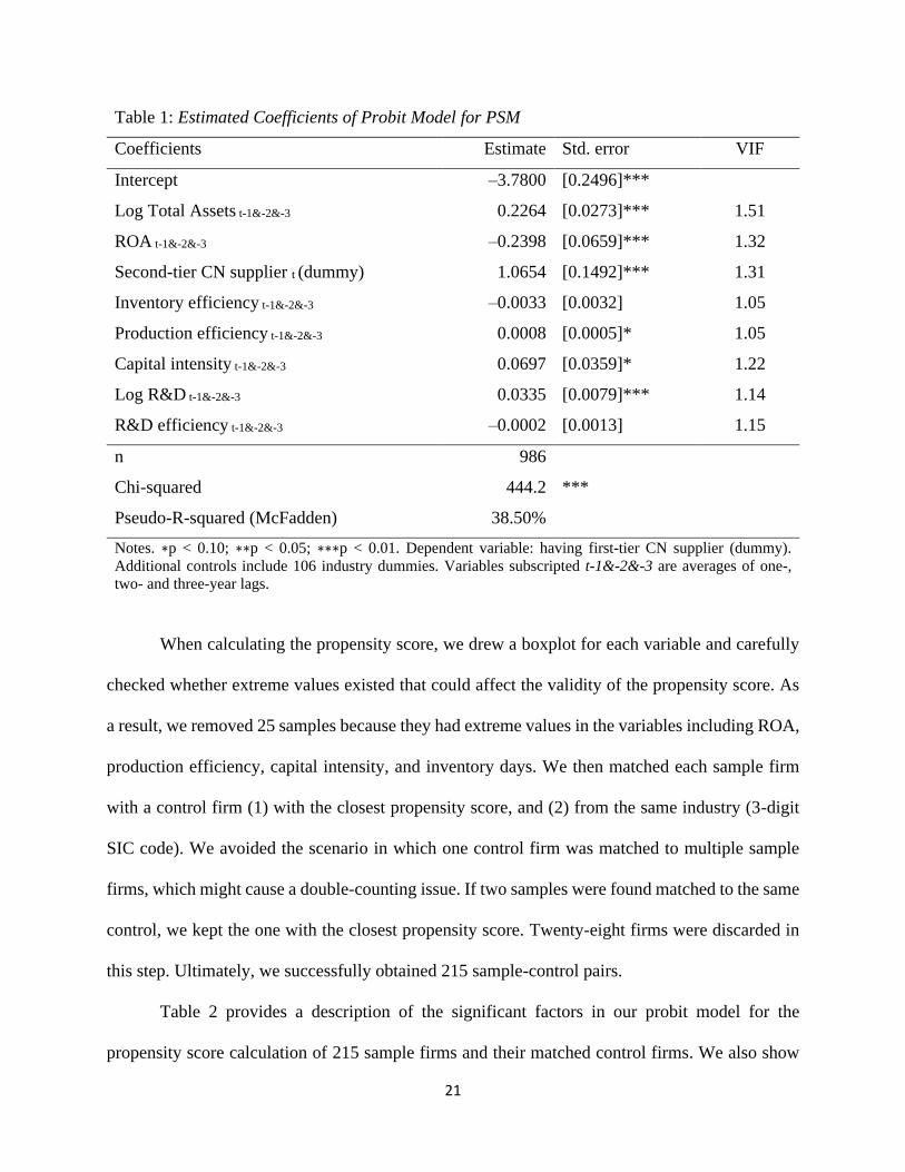
21

Table 1: Estimated Coefficients of Probit Model for PSM

Coefficients Estimate Std. error VIF

Intercept –3.7800 [0.2496]***

Log Total Assets t-1&-2&-3 0.2264 [0.0273]*** 1.51

ROA t-1&-2&-3 –0.2398 [0.0659]*** 1.32

Second-tier CN supplier t (dummy) 1.0654 [0.1492]*** 1.31

Inventory efficiency t-1&-2&-3 –0.0033 [0.0032] 1.05

Production efficiency t-1&-2&-3 0.0008 [0.0005]* 1.05

Capital intensity t-1&-2&-3 0.0697 [0.0359]* 1.22

Log R&D t-1&-2&-3 0.0335 [0.0079]*** 1.14

R&D efficiency t-1&-2&-3 –0.0002 [0.0013] 1.15

n 986

Chi-squared 444.2 ***

Pseudo-R-squared (McFadden) 38.50%

Notes. ∗p < 0.10; ∗∗p < 0.05; ∗∗∗p < 0.01. Dependent variable: having first-tier CN supplier (dummy).

Additional controls include 106 industry dummies. Variables subscripted t-1&-2&-3 are averages of one-,

two- and three-year lags.

When calculating the propensity score, we drew a boxplot for each variable and carefully

checked whether extreme values existed that could affect the validity of the propensity score. As

a result, we removed 25 samples because they had extreme values in the variables including ROA,

production efficiency, capital intensity, and inventory days. We then matched each sample firm

with a control firm (1) with the closest propensity score, and (2) from the same industry (3-digit

SIC code). We avoided the scenario in which one control firm was matched to multiple sample

firms, which might cause a double-counting issue. If two samples were found matched to the same

control, we kept the one with the closest propensity score. Twenty-eight firms were discarded in

this step. Ultimately, we successfully obtained 215 sample-control pairs.

Table 2 provides a description of the significant factors in our probit model for the

propensity score calculation of 215 sample firms and their matched control firms. We also show

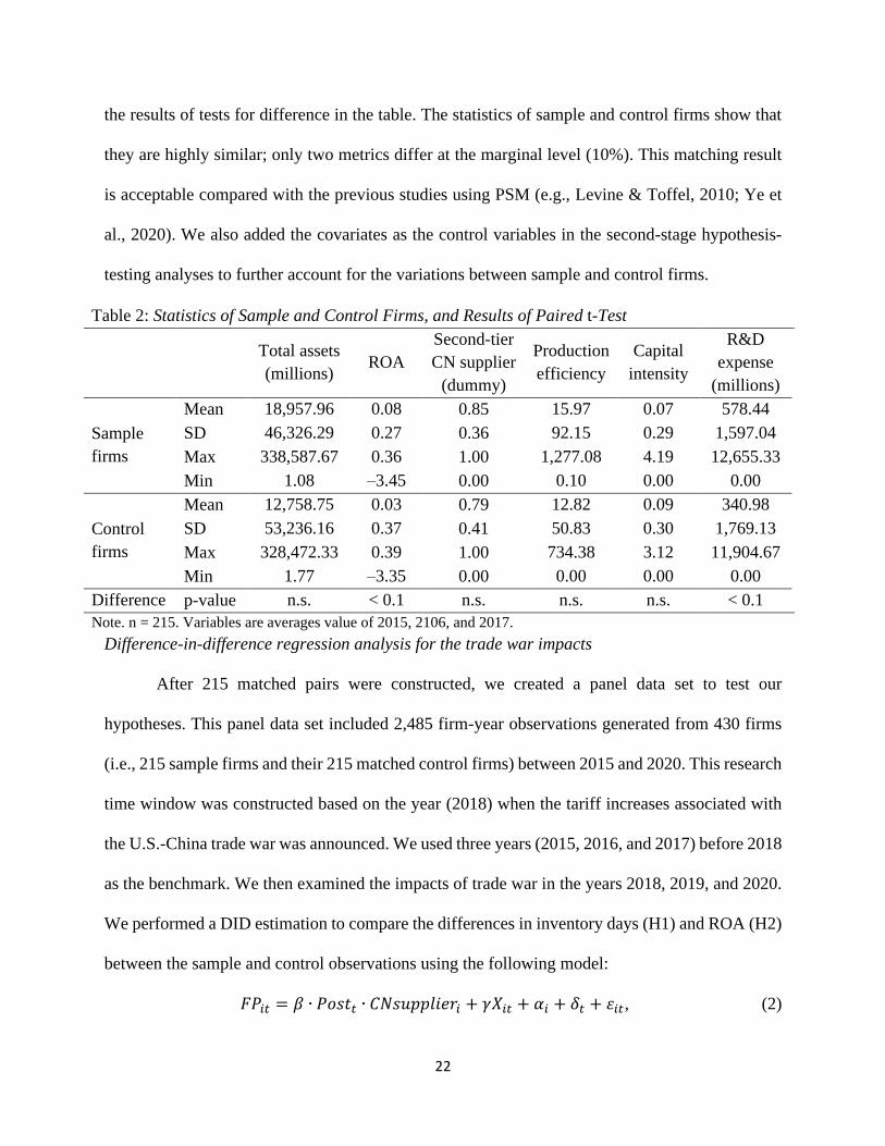
22

the results of tests for difference in the table. The statistics of sample and control firms show that

they are highly similar; only two metrics differ at the marginal level (10%). This matching result

is acceptable compared with the previous studies using PSM (e.g., Levine & Toffel, 2010; Ye et

al., 2020). We also added the covariates as the control variables in the second-stage hypothesis-

testing analyses to further account for the variations between sample and control firms.

Table 2: Statistics of Sample and Control Firms, and Results of Paired t-Test

Total assets

(millions) ROA

Second-tier

CN supplier

(dummy)

Production

efficiency

Capital

intensity

R&D

expense

(millions)

Sample

firms

Mean 18,957.96 0.08 0.85 15.97 0.07 578.44

SD 46,326.29 0.27 0.36 92.15 0.29 1,597.04

Max 338,587.67 0.36 1.00 1,277.08 4.19 12,655.33

Min 1.08 –3.45 0.00 0.10 0.00 0.00

Control

firms

Mean 12,758.75 0.03 0.79 12.82 0.09 340.98

SD 53,236.16 0.37 0.41 50.83 0.30 1,769.13

Max 328,472.33 0.39 1.00 734.38 3.12 11,904.67

Min 1.77 –3.35 0.00 0.00 0.00 0.00

Difference p-value n.s. < 0.1 n.s. n.s. n.s. < 0.1

Note. n = 215. Variables are averages value of 2015, 2106, and 2017.

Difference-in-difference regression analysis for the trade war impacts

After 215 matched pairs were constructed, we created a panel data set to test our

hypotheses. This panel data set included 2,485 firm-year observations generated from 430 firms

(i.e., 215 sample firms and their 215 matched control firms) between 2015 and 2020. This research

time window was constructed based on the year (2018) when the tariff increases associated with

the U.S.-China trade war was announced. We used three years (2015, 2016, and 2017) before 2018

as the benchmark. We then examined the impacts of trade war in the years 2018, 2019, and 2020.

We performed a DID estimation to compare the differences in inventory days (H1) and ROA (H2)

between the sample and control observations using the following model:

𝐹𝑃𝑖𝑡 = 𝛽 ∙ 𝑃𝑜𝑠𝑡𝑡 ∙ 𝐶𝑁𝑠𝑢𝑝𝑝𝑙𝑖𝑒𝑟𝑖 + 𝛾𝑋𝑖𝑡 + 𝛼𝑖 + 𝛿𝑡 + 휀𝑖𝑡, (2)

23

where the dependent variable 𝐹𝑃𝑖𝑡 refers to the firm’s performance (i.e., inventory days or ROA)

of firm i in the year t. 𝑃𝑜𝑠𝑡𝑡 equals 1 if the year t corresponds to the year on or after the 2018

announcement of tariff increases (i.e., 2018, 2019, and 2020); otherwise, it equals 0. 𝐶𝑁𝑠𝑢𝑝𝑝𝑙𝑖𝑒𝑟𝑖

equals 1 if firm i has first-tier Chinese suppliers, and equals 0 otherwise. Thus, the interaction term

𝑃𝑜𝑠𝑡𝑡 ∙ 𝐶𝑁𝑠𝑢𝑝𝑝𝑙𝑖𝑒𝑟𝑖 equals 1 for the observations on or after 2018 of firm i who had first-tier

Chinese suppliers before the trade war, and 𝛽 should capture the change in the firm’s performance

after the tariff list is announced. We included the vector 𝑋𝑖𝑡 to control for the firm-level

characteristics controlled in the selection model, namely, total assets (natural logarithm

transformed), capital intensity, inventory efficiency, production efficiency, log of R&D

expenditure, and R&D efficiency to increase the validity of our results. The measurements of these

control variables were the same as we use in PSM (see Appendix A2). Total assets were used to

control for firm size, because larger firms may be affected by supply chain disruption easily as

they seem to be more often involved in complex supply chains (Revilla & Saenz, 2017). Capital

intensity includes a firm’s capital investment in production and information technology, which

may improve firm’s financial and inventory performance (Steven et al., 2014). Inventory

efficiency and production efficiency were included to control for the firm’s operating efficiency.

Efficient firms may have fewer slacks available to respond to supply chain disruptions (Wiengarten

et al., 2017). R&D expenditure is included because the firm’s investment on innovativeness is

related to the firm’s economic growth (Zahra et al., 2000). R&D efficiency indicates a firm’s

investment efficiency in research and development, which may affect its profitability (Cho &

Pucik, 2005). We also included the supply complexity metrics in 𝑋𝑖𝑡, including vertical integration,

horizontal complexity, spatial complexity, and cooperative complexity. The measurements of

these variables will be described in the next section. We also included the firm’s number of second-

24

tier suppliers per first-tier suppliers (vertical complexity) to control for the indirect supply chain

effect. In addition, we controlled for the firm fixed effect— 𝛼𝑖— and the year fixed effect: 𝛿𝑡. 휀𝑖𝑡

is the error term. 𝑃𝑜𝑠𝑡𝑡 and 𝐶𝑁𝑠𝑢𝑝𝑝𝑙𝑖𝑒𝑟𝑖 are omitted in the model because we have controlled for

the firm and year fixed effects (Levine & Toffel, 2010). In the above specified model, we expected

to capture a positive coefficient in 𝛽 in the inventory days model and a negative coefficient in the

ROA model. These can capture the abnormal negative impacts experienced by the sample firms

amidst trade war and examine H1 and H2.

Subsample difference-in-difference analysis for supply structure

The intent of hypotheses H3–H6 is to examine whether firms with a more complex supply structure

suffer more from the tariff increases caused by the trade war. These hypotheses can be examined

in two methods. First, we can insert an interaction term between the supply structure factors and

the 𝑃𝑜𝑠𝑡𝑡 ∙ 𝐶𝑁𝑠𝑢𝑝𝑝𝑙𝑖𝑒𝑟𝑖 and examine the significance in the coefficient. However, this treatment

would create a three-way interaction term among supply structure factors, Postt and CNsupplieri.

These increase the difficulty of the interpretation of the coefficient and thus the marginal effects.

Another method is to divide the subsamples according to the high and low levels of the supply

structure factors, namely, vertical integration and horizontal, spatial, and cooperative complexity.

The subsample analysis approach is arguably more appropriate for indicating the “strength”

of moderators across various scenarios (Arnold, 1982; Su et al., 2015; Ye et al., 2020). In H3 to

H6, we hypothesized that the level of outsourcing activities and complexity accentuate the impacts

of the trade war on a U.S. firm with Chinese suppliers. So, we intend to test the “strength” of the

moderators. In addition, the coefficients in the divided group can be easily interpreted, which

facilitates the calculation of the marginal effects for managerial implications. This approach is

25

consistent with the previous OM literature using a DID regression technique (e.g., Gu et al., 2017;

Soysal et al., 2019; Ye et al., 2020).

Therefore, we used the subsample analysis to examine H3 to H6. Specifically, for each

hypothesis testing, we divided the sample firms into two groups (i.e., low-level group and high-

level group) based on the yearly industry median of the moderators (i.e., vertical integration,

horizontal complexity, spatial complexity, and cooperative complexity). We then reran the

regression by using each of the groups to examine H3 to H6. As a robustness check, we also

followed Levine & Toffel (2010) to create interaction terms to verify our conclusions (see

robustness check section). We used ROA as the dependent variable for these analyses because this

indicator was widely used as the bottom-line firm performance metric (e.g., Lo et al., 2014; Swift

et al., 2019). The data of supply structure factors were taken at year 2017. They were measured in

the following ways:

Vertical integration was measured according to a method developed by Frésard et al.

(2020).1 Hendricks et al. (2009) had applied an industry-level measure, vertical relatedness, based

on the “Use Table” of the input-output (IO) table provided by the Bureau of Economic Analysis

(BEA), but the authors stated that “it would be ideal to use firm-specific data to compute the

vertical relatedness at the firm level” (p. 239). Recently, Frésard et al. (2020) developed a firm-

level vertical integration measure built on the IO table and calculated using a textual analysis of

an individual firm’s business description from its 10-K disclosure. The measurement was based

on the assumption that a firm’s product vocabularies are vertically related to the same firm’s other

product vocabularies. The vertical integration score is higher when the product vocabulary in the

1 The variable can be obtained from http://faculty.marshall.usc.edu/Gerard-

Hoberg/FresardHobergPhillipsDataSite/index.html.

26

description spans vertically related markets (Frésard et al., 2020). The validity of the variable was

verified by its significant statistical correlation with firms mentioned using the words “vertical

integration” and “vertically integrated” in their 10-K report (Frésard et al., 2020). A higher value

of vertical integration indicated that the firm was offering products that were more vertically

related.

Horizontal complexity was measured by the firm’s number of first-tier suppliers (Bode &

Wagner, 2015; Dong et al., 2020). This measurement reflects the multiplicity of the firm’s supply

base (Choi & Krause, 2006; Sharma et al., 2020). We excluded the U.S. and Chinese suppliers in

this measurement to better reflect the sense of backup suppliers that would be less directly affected

by the U.S.-China trade war.

Spatial complexity is the geographical spread of a firm’s suppliers (Bode & Wagner, 2015).

We followed Lu and Shang (2017) to measure spatial complexity as the number of countries or

regions where a firm’s suppliers were located. This measurement reflects the diversity of the

supply base (Sharma et al., 2020). We excluded U.S. and Chinese suppliers to capture the firm’s

international supply network. This measure assumes that widespread supply bases should increase

the difficulty of coordinating production and create more policy uncertainties (Lu & Shang, 2017;

Vachon & Klassen, 2002).

Cooperative complexity was measured by the level of connection among the firm’s first-

tier suppliers (Dong et al., 2020; Lu & Shang, 2017). Specifically, we counted the number of actual

links among first-tier suppliers. This number was then divided by the maximum number of possible

links among first-tier suppliers to control for the network size. This measurement reflects the

interrelatedness of the supply base (Krause & Choi, 2006).

27

Table 3. Correlation table of variables in DID analysis.

1 2 3 4 5 6 7 8 9 10 11

1. Post*CNsupplier

2. log Total Assets 0.25***

3. Capital Intensity -0.03 0.01

4. Inventory

Efficiency -0.01 0.12*** 0.09***

5. Production

Efficiency -0.02 -0.18*** -0.04* 0.05**

6. Log R&D 0.13*** 0.21*** -0.08*** -0.02 -0.14***

7. R&D Efficiency 0.02 0.09*** -0.38*** 0.03 0.01 0

8. Vertical

Complexity -0.13*** -0.04* 0.04** 0.02 0.01 -0.03* -0.05***

9. Vertical

Integration -0.02 0.11*** -0.06*** -0.1*** -0.06*** -0.06*** 0.02 -0.07***

10. Horizontal

Complexity 0.04* 0.36*** 0.01 0.15*** 0.01 0.17 0.01 -0.01 -0.04***

11. Spatial

Complexity 0.04** 0.46*** 0.01 0.16*** -0.02 0.18 0.01 0.03 -0.02 0.76***

12. Cooperative

Complexity -0.06*** -0.06*** -0.01 0.01 0 -0.01 0.01 0.17*** -0.02 -0.06*** -0.06***

Note. ∗p<0.10; ∗∗p<0.05; ∗∗∗p<0.01. n=2485

28

Analysis of Results

Table 4: Results of DID Analysis

Inventory days ROA

Coefficients Estimate Std. error Estimate Std. error

Post*CN supplier 8.0331 [3.1389]** –0.0389 [0.0162]**

Log total assets –4.2715 [0.5734]*** 0.0703 [0.0030]***

Capital intensity –3.7736 [4.0110] –0.0808 [0.0208]***

Inventory efficiency –1.7510 [0.0918]*** 0.0004 [0.0005]

Production efficiency –0.0388 [0.0168]** 0.0001 [0.0001]

Log R&D 1.0410 [0.1701]*** –0.0008 [0.0009]

R&D efficiency 0.3785 [0.1084]*** 0.0026 [0.0006]***

Vertical complexity –0.0580 [0.0307]* –0.0005 [0.0002]***

Vertical integration –587.5539 [81.6706]*** 0.4723 [0.4226]

Horizontal complexity 0.0467 [0.0647] –0.0002 [0.0003]

Spatial complexity –0.7037 [0.3491]** –0.0083 [0.0018]***

Cooperative complexity –22.9997 [15.1911] 0.0209 [0.0786]

n 2485 2485 R-squared 20.54% 23.17% Adj. R-squared 19.99% 22.64% F-statistic 53.15 *** 61.99 ***

Note. ∗p < 0.10; ∗∗p < 0.05; ∗∗∗p < 0.01. Firm and year fixed effects were controlled.

Table 3 presents the correlation of the indicators while Table 4 presents the results for examining

H1 and H2 by considering the coefficients of interaction term 𝑃𝑜𝑠𝑡𝑡 ∙ 𝐶𝑁𝑠𝑢𝑝𝑝𝑙𝑖𝑒𝑟𝑖. The inventory

days model shows that the interaction term 𝑃𝑜𝑠𝑡𝑡 ∙ 𝐶𝑁𝑠𝑢𝑝𝑝𝑙𝑖𝑒𝑟𝑖 is significantly positive (b =

8.0331, p < 0.05), indicating that the inventory days measure increased by 8.03 days (8.3%

according to the same mean) in sample firms during the trade war. Thus, H1 is supported. The

results suggest that the tariff induced a sense of policy uncertainty for U.S. firms with Chinese

suppliers. These firms might have responded by initiating relocations and advance purchasing to

mitigate the uncertainty. However, these responses undermined inventory turnover. The increased

number of inventory days echoed the increase of the United States’ trade deficit, which reached a

29

10-year high at $621 billion in 2018 (Dmitrieva, 2019), which indicates that U.S. firms with

Chinese suppliers were in a buying binge triggered by uncertainty about future tariff increases

(Naidu & Baertlein, 2018).

The ROA model of Table 4 shows that the interaction term 𝑃𝑜𝑠𝑡𝑡 ∙ 𝐶𝑁𝑠𝑢𝑝𝑝𝑙𝑖𝑒𝑟𝑖 is

significantly negative (b = –0.0389, p < 0.05), indicating a decrease in ROA of about 3.89% for

the sample firms during the trade war. Thus, H2 is supported. This result suggests that the tariffs

were undermining U.S. firms’ profitability. The deterioration appeared after the tariff went into

effect, and firms were unable to recover even 2 years after the tariff was imposed.

Tables 5 to 8 present the results of our subsample DID analysis for comparing the levels

of vertical integration, horizontal complexity, spatial complexity, and cooperative complexity,

respectively. In Table 5, the coefficient of interaction term 𝑃𝑜𝑠𝑡𝑡 ∙ 𝐶𝑁𝑠𝑢𝑝𝑝𝑙𝑖𝑒𝑟𝑖 in groups with

low levels is significantly negative (b = –0.0742, p < 0.05), indicating that the ROA performance

of firms with Chinese suppliers that have a low level of vertical integration was 7.42% lower

compared to firms without Chinese suppliers. However, the coefficient of interaction term 𝑃𝑜𝑠𝑡𝑡 ∙

𝐶𝑁𝑠𝑢𝑝𝑝𝑙𝑖𝑒𝑟𝑖 in groups with high levels is not statistically significant (p > 0.1), indicating that

firms with a high level of vertical integration did not experience a decline in ROA during the trade

war. These contrasting results support H3.

Table 6 presents the results of horizontal complexity. The interaction term 𝑃𝑜𝑠𝑡𝑡 ∙

𝐶𝑁𝑠𝑢𝑝𝑝𝑙𝑖𝑒𝑟𝑖 in the high-level group is significantly negative (b = –0.0392, p < 0.05), which

indicates that the ROA performance of firms with Chinese suppliers having a high level of

horizontal complexity was 3.92% lower compared to firms without Chinese suppliers. However,

the coefficient of interaction term 𝑃𝑜𝑠𝑡𝑡 ∙ 𝐶𝑁𝑠𝑢𝑝𝑝𝑙𝑖𝑒𝑟𝑖 in the low-level group is not statistically

30

significant (p > 0.1), which indicates that firms with fewer direct suppliers suffered little from the

trade war. Thus, H4 is supported.

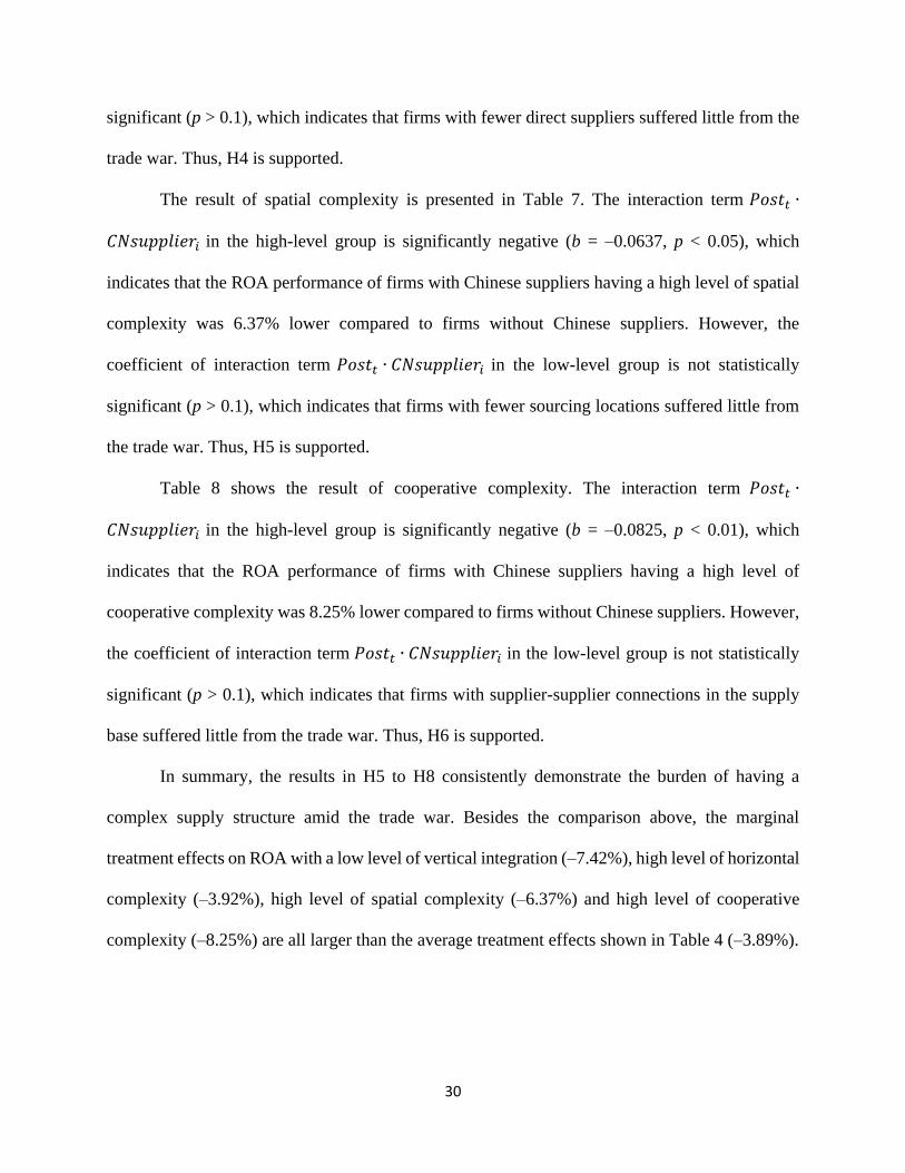
The result of spatial complexity is presented in Table 7. The interaction term 𝑃𝑜𝑠𝑡𝑡 ∙


indicates that the ROA performance of firms with Chinese suppliers having a high level of spatial

complexity was 6.37% lower compared to firms without Chinese suppliers. However, the

coefficient of interaction term 𝑃𝑜𝑠𝑡𝑡 ∙ 𝐶𝑁𝑠𝑢𝑝𝑝𝑙𝑖𝑒𝑟𝑖 in the low-level group is not statistically

significant (p > 0.1), which indicates that firms with fewer sourcing locations suffered little from

the trade war. Thus, H5 is supported.

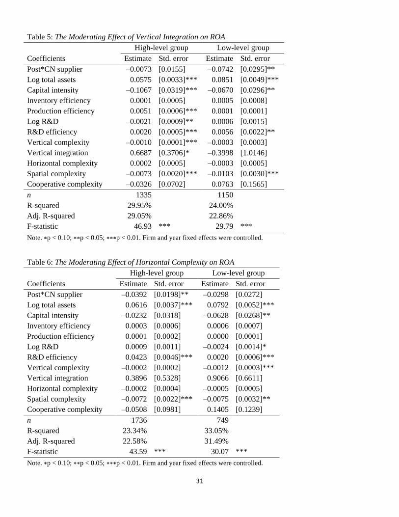
Table 8 shows the result of cooperative complexity. The interaction term 𝑃𝑜𝑠𝑡𝑡 ∙


indicates that the ROA performance of firms with Chinese suppliers having a high level of

cooperative complexity was 8.25% lower compared to firms without Chinese suppliers. However,

the coefficient of interaction term 𝑃𝑜𝑠𝑡𝑡 ∙ 𝐶𝑁𝑠𝑢𝑝𝑝𝑙𝑖𝑒𝑟𝑖 in the low-level group is not statistically

significant (p > 0.1), which indicates that firms with supplier-supplier connections in the supply

base suffered little from the trade war. Thus, H6 is supported.

In summary, the results in H5 to H8 consistently demonstrate the burden of having a

complex supply structure amid the trade war. Besides the comparison above, the marginal

treatment effects on ROA with a low level of vertical integration (–7.42%), high level of horizontal

complexity (–3.92%), high level of spatial complexity (–6.37%) and high level of cooperative

complexity (–8.25%) are all larger than the average treatment effects shown in Table 4 (–3.89%).

31

Table 5: The Moderating Effect of Vertical Integration on ROA

High-level group Low-level group


Post*CN supplier –0.0073 [0.0155] –0.0742 [0.0295]**

Log total assets 0.0575 [0.0033]*** 0.0851 [0.0049]***

Capital intensity –0.1067 [0.0319]*** –0.0670 [0.0296]**

Inventory efficiency 0.0001 [0.0005] 0.0005 [0.0008]

Production efficiency 0.0051 [0.0006]*** 0.0001 [0.0001]

Log R&D –0.0021 [0.0009]** 0.0006 [0.0015]

R&D efficiency 0.0020 [0.0005]*** 0.0056 [0.0022]**

Vertical complexity –0.0010 [0.0001]*** –0.0003 [0.0003]

Vertical integration 0.6687 [0.3706]* –0.3998 [1.0146]

Horizontal complexity 0.0002 [0.0005] –0.0003 [0.0005]

Spatial complexity –0.0073 [0.0020]*** –0.0103 [0.0030]***


n 1335 1150

R-squared 29.95% 24.00% Adj. R-squared 29.05% 22.86% F-statistic 46.93 *** 29.79 ***


Table 6: The Moderating Effect of Horizontal Complexity on ROA



Post*CN supplier –0.0392 [0.0198]** –0.0298 [0.0272]

Log total assets 0.0616 [0.0037]*** 0.0792 [0.0052]***

Capital intensity –0.0232 [0.0318] –0.0628 [0.0268]**


Production efficiency 0.0001 [0.0002] 0.0000 [0.0001]

Log R&D 0.0009 [0.0011] –0.0024 [0.0014]*

R&D efficiency 0.0423 [0.0046]*** 0.0020 [0.0006]***

Vertical complexity –0.0002 [0.0002] –0.0012 [0.0003]***

Vertical integration 0.3896 [0.5328] 0.9066 [0.6611]

Horizontal complexity –0.0002 [0.0004] –0.0005 [0.0005]

Spatial complexity –0.0072 [0.0022]*** –0.0075 [0.0032]**


n 1736 749



32

Table 7: The Moderating Effect of Spatial Complexity on ROA



Post*CN supplier –0.0637 [0.0254]** –0.0240 [0.0196]

Log total assets 0.0768 [0.0049]*** 0.0662 [0.0037]***



Production efficiency 0.0001 [0.0002] 0.0000 [0.0001]

Log R&D 0.0015 [0.0013] –0.0028 [0.0012]**

R&D efficiency 0.0325 [0.0052]*** 0.0023 [0.0005]***

Vertical complexity –0.0003 [0.0003] –0.0007 [0.0002]***

Vertical integration 0.2424 [0.6652] 0.8231 [0.5097]


Spatial complexity –0.0073 [0.0027]*** –0.0076 [0.0024]***


n 1258 1227



Table 8: The Moderating Effect of Cooperative Complexity on ROA



Post*CN supplier –0.0825 [0.0235]*** 0.0154 [0.0214]

Log total assets 0.0699 [0.0043]*** 0.0684 [0.0042]***



Production efficiency 0.0001 [0.0001] –0.0001 [0.0003]

Log R&D 0.0001 [0.0013] –0.0009 [0.0012]

R&D efficiency 0.0425 [0.0074]*** 0.0023 [0.0005]***

Vertical complexity 0.0000 [0.0002] –0.0011 [0.0002]***

Vertical integration 0.0607 [0.6369] 0.9241 [0.5446]*


Spatial complexity –0.0067 [0.0026]** –0.0090 [0.0024]***

Cooperative complexity 0.0264 [0.1122] 0.0397 [0.1071]

n 1378 1107



33

Robustness Checks

We conducted several additional tests with alternative specifications, measurement, and

grouping approach to check the robustness of our findings. We plotted the mean ROA and

inventory days performance in Figure 2 and conducted a common trend analysis to check the

parallel assumption for DID analysis. We also plotted the results of placebo test based on firms

with “false” Chinese suppliers in 2018 under the tariff changes in Figure 3. For moderating factors,

we dropped the samples between 45th to 55th percentile to achieve great separation. We also

applied subgroup dummies to create a three-way interaction term to confirm our moderating effects

in Table 11. Overall, these tests provide consistent evidence on our main results. We discussed the

detailed procedures as below.

Parallel assumption for DID analysis

The assumption for DID analysis to capture any treatment effect is parallel performance,

which requires that there be a common trend in dependent variables (i.e., inventory days and ROA)

between the sample and control groups before the announcement year of the tariff list. We first

followed Song et al. (2020) to visualize the dependent variables for the sample and control groups

in Figures 2a and 2b. The average inventory days and ROA for the sample and control firms

indicate a consistent difference between the two groups before the tariff lists were announced.

We also performed an additional common trend analysis using the following relative time

model (Angrist and Pischke, 2008; Song et al., 2020):

𝑃𝑖𝑡 = 𝛽 ∙ 𝐶𝑁𝑠𝑢𝑝𝑝𝑙𝑖𝑒𝑟𝑖 + ∑ 𝜅𝑡 ∙ 𝐶𝑁𝑠𝑢𝑝𝑝𝑙𝑖𝑒𝑟𝑖2020𝑡=2015 ∙ 𝐷𝑖𝑡 + 𝛾𝑋𝑖𝑡 + 𝛼𝑖 + 𝛿𝑡 + 휀𝑖𝑡, (3)

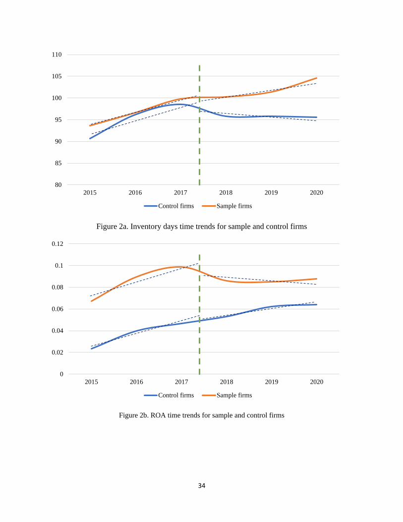
34

Figure 2a. Inventory days time trends for sample and control firms

Figure 2b. ROA time trends for sample and control firms

80

85

90

95

100

105

110

2015 2016 2017 2018 2019 2020

Control firms Sample firms

0

0.02

0.04

0.06

0.08

0.1

0.12

2015 2016 2017 2018 2019 2020

Control firms Sample firms

35

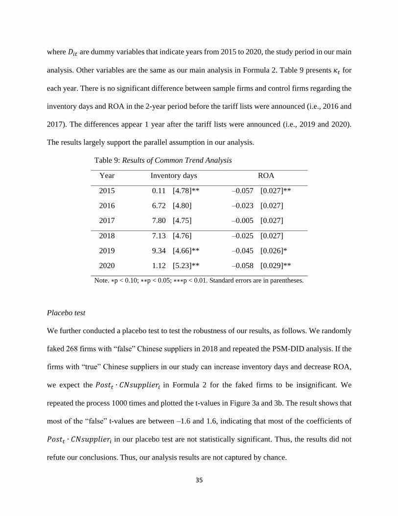
where 𝐷𝑖𝑡 are dummy variables that indicate years from 2015 to 2020, the study period in our main

analysis. Other variables are the same as our main analysis in Formula 2. Table 9 presents 𝜅𝑡 for

each year. There is no significant difference between sample firms and control firms regarding the

inventory days and ROA in the 2-year period before the tariff lists were announced (i.e., 2016 and

2017). The differences appear 1 year after the tariff lists were announced (i.e., 2019 and 2020).

The results largely support the parallel assumption in our analysis.

Table 9: Results of Common Trend Analysis

Year Inventory days ROA

2015 0.11 [4.78]** –0.057 [0.027]**

2016 6.72 [4.80] –0.023 [0.027]

2017 7.80 [4.75] –0.005 [0.027]

2018 7.13 [4.76] –0.025 [0.027]

2019 9.34 [4.66]** –0.045 [0.026]*

2020 1.12 [5.23]** –0.058 [0.029]**

Note. ∗p < 0.10; ∗∗p < 0.05; ∗∗∗p < 0.01. Standard errors are in parentheses.

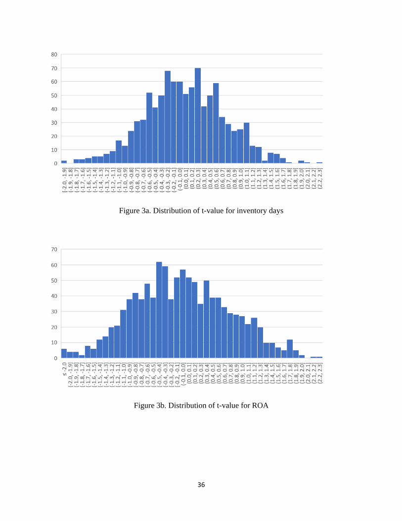
Placebo test

We further conducted a placebo test to test the robustness of our results, as follows. We randomly

faked 268 firms with “false” Chinese suppliers in 2018 and repeated the PSM-DID analysis. If the

firms with “true” Chinese suppliers in our study can increase inventory days and decrease ROA,

we expect the 𝑃𝑜𝑠𝑡𝑡 ∙ 𝐶𝑁𝑠𝑢𝑝𝑝𝑙𝑖𝑒𝑟𝑖 in Formula 2 for the faked firms to be insignificant. We

repeated the process 1000 times and plotted the t-values in Figure 3a and 3b. The result shows that

most of the “false” t-values are between –1.6 and 1.6, indicating that most of the coefficients of

𝑃𝑜𝑠𝑡𝑡 ∙ 𝐶𝑁𝑠𝑢𝑝𝑝𝑙𝑖𝑒𝑟𝑖 in our placebo test are not statistically significant. Thus, the results did not

refute our conclusions. Thus, our analysis results are not captured by chance.

36

Figure 3a. Distribution of t-value for inventory days

Figure 3b. Distribution of t-value for ROA

37

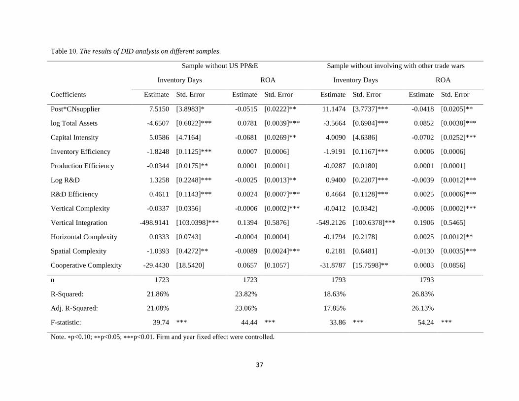
Table 10. The results of DID analysis on different samples.

Sample without US PP&E Sample without involving with other trade wars

Inventory Days ROA Inventory Days ROA

Coefficients Estimate Std. Error Estimate Std. Error Estimate Std. Error Estimate Std. Error

Post*CNsupplier 7.5150 [3.8983]* -0.0515 [0.0222]** 11.1474 [3.7737]*** -0.0418 [0.0205]**

log Total Assets -4.6507 [0.6822]*** 0.0781 [0.0039]*** -3.5664 [0.6984]*** 0.0852 [0.0038]***

Capital Intensity 5.0586 [4.7164] -0.0681 [0.0269]** 4.0090 [4.6386] -0.0702 [0.0252]***

Inventory Efficiency -1.8248 [0.1125]*** 0.0007 [0.0006] -1.9191 [0.1167]*** 0.0006 [0.0006]

Production Efficiency -0.0344 [0.0175]** 0.0001 [0.0001] -0.0287 [0.0180] 0.0001 [0.0001]

Log R&D 1.3258 [0.2248]*** -0.0025 [0.0013]** 0.9400 [0.2207]*** -0.0039 [0.0012]***

R&D Efficiency 0.4611 [0.1143]*** 0.0024 [0.0007]*** 0.4664 [0.1128]*** 0.0025 [0.0006]***

Vertical Complexity -0.0337 [0.0356] -0.0006 [0.0002]*** -0.0412 [0.0342] -0.0006 [0.0002]***

Vertical Integration -498.9141 [103.0398]*** 0.1394 [0.5876] -549.2126 [100.6378]*** 0.1906 [0.5465]

Horizontal Complexity 0.0333 [0.0743] -0.0004 [0.0004] -0.1794 [0.2178] 0.0025 [0.0012]**

Spatial Complexity -1.0393 [0.4272]** -0.0089 [0.0024]*** 0.2181 [0.6481] -0.0130 [0.0035]***

Cooperative Complexity -29.4430 [18.5420] 0.0657 [0.1057] -31.8787 [15.7598]** 0.0003 [0.0856]

n 1723 1723 1793 1793

R-Squared: 21.86%

23.82%

18.63%

26.83%

Adj. R-Squared: 21.08%

23.06%

17.85%

26.13%

F-statistic: 39.74 *** 44.44 *** 33.86 *** 54.24 ***

Note. ∗p<0.10; ∗∗p<0.05; ∗∗∗p<0.01. Firm and year fixed effect were controlled.

38

Variations in samples

In addition, we fine-tuned our sample to conduct a DID regression analysis. First, U.S. firms with

U.S. PP&E in our sample may not be affected by the tariff changes as they may purchase raw

materials that are not on the tariff lists and produce finished goods in their US plants. We therefore

excluded those samples and redid the analysis. Second, the tariffs between the United States and

other countries could also affect the results. Therefore, we eliminated the samples of U.S. firms

with suppliers in other countries engaged in a trade war with the United States during our study

period. The analysis of the results is largely identical to those of our main results. We present the

results in Table 10.

Additional tests for subsample DID analysis

Dividing the samples into subgroups may not achieve clear separation between firms with

higher versus lower integration and complexity levels because some firms’ integration and

complexity levels may be close to the median levels. We therefore dropped the samples between

45th to 55th percentile for integration and complexity levels to achieve great separation (Su et al.,

2015). We reran the analysis based on the subsamples below 45th percentile (low-level groups)

and above 55th percentile (high-level groups), and the results are identical as those of our main

analysis. The results are presented in Appendix B Table B1 (Vertical Integration), B2 (Horizontal

Complexity), B3 (Spatial Complexity) and B4 (Cooperative Complexity).

The difficulty of interpreting coefficients of three-way interaction terms motivated us to

use subsample analysis to examine H3 to H6. To further cross-examine the robustness of our

subsample analysis results, we followed Levine and Toffel (2010) to apply the interaction terms

and the below estimation model:

39

𝐹𝑃𝑖𝑡 = 𝛽 ∙ 𝑃𝑜𝑠𝑡𝑡 ∙ 𝐶𝑁𝑠𝑢𝑝𝑝𝑙𝑖𝑒𝑟𝑖 ∙ 𝐻𝑖𝑔ℎ𝐺𝑟𝑜𝑢𝑝𝑖 + 𝜅 ∙ 𝑃𝑜𝑠𝑡𝑡 ∙ 𝐶𝑁𝑠𝑢𝑝𝑝𝑙𝑖𝑒𝑟𝑖 ∙ 𝐿𝑜𝑤𝐺𝑟𝑜𝑢𝑝𝑖 +

𝛾𝑋𝑖𝑡 + 𝛼𝑖 + 𝛿𝑡 + 휀𝑖𝑡 (4)

where 𝐻𝑖𝑔ℎ𝐺𝑟𝑜𝑢𝑝𝑖 are dummy variables that indicate firm i belongs to high-level group,

𝐿𝑜𝑤𝐺𝑟𝑜𝑢𝑝𝑖 are dummy variables that indicate firm i belongs to low-level group. Other variables

are the same as our main analysis in formula 2. So 𝛽 and 𝜅 should capture the changes in firm’s

performance in high- and low-level groups after the tariff lists were announced. Model 1, 2, 3, and

4 in Table 11 show the results of vertical integration, horizontal complexity, spatial complexity,

and cooperative complexity respectively. Post*CNsupplier*Low Vertical Integration,

Post*CNsupplier*High Horizontal Complexity, Post*CNsupplier*High Spatial Complexity, and

Post*CNsupplier*High Cooperative Complexity are significantly negative (p < 0.01), which are

identical to those of our main analysis.

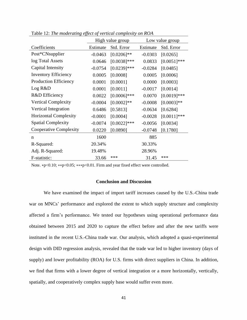
In addition, using horizontal complexity to test H4 may ignore the effects of second tier

suppliers in a supply chain. We therefore applied subsample DID analysis on vertical complexity

to replace horizontal complexity. In Table 12, the interaction term 𝑃𝑜𝑠𝑡𝑡 ∙ 𝐶𝑁𝑠𝑢𝑝𝑝𝑙𝑖𝑒𝑟𝑖 in high-

level group is significantly negative (b = -0.0463, p < 0.05), indicating that firms with Chinese

suppliers having a high level of vertical complexity reduce the ROA performance by 4.63%

compared to firms without Chinese suppliers. However, the coefficient of interaction term 𝑃𝑜𝑠𝑡𝑡 ∙

𝐶𝑁𝑠𝑢𝑝𝑝𝑙𝑖𝑒𝑟𝑖 in low-level group is not statistically significant (p > 0.1), indicating that firms with

fewer direct and indirect suppliers suffered little from the trade war. Thus, H4 is still supported.

40

Table 11. The moderating effects on ROA

Model 1

Vertical Integration

Model 2

Horizontal Complexity

Model 3

Spatial Complexity

Model 4

Cooperative Complexity

Post*CNsupplier*High Vertical Integration -0.0282 [0.0192] - - - - - -

Post*CNsupplier*Low Vertical Integration -0.0525 [0.0200]*** - - - - - -

Post*CNsupplier*High Horizontal Complexity - - -0.0494 [0.0179]*** - - - -

Post*CNsupplier*Low Horizontal Complexity - - -0.0142 [0.0229] - - - -

Post*CNsupplier*High Spatial Complexity - - - - -0.0817 [0.0198]*** - -

Post*CNsupplier*Low Spatial Complexity - - - - -0.0106 [0.0193] - -

Post*CNsupplier*High Cooperative Complexity - - - - - - -0.0746 [0.0192]***

Post*CNsupplier*Low Cooperative Complexity - - - - - - 0.0017 [0.0199]

log Total Assets 0.0707 [0.0029]*** 0.0706 [0.0030]*** 0.0673 [0.0029]*** 0.0714 [0.0030]***

Capital Intensity -0.0821 [0.0207]*** -0.0808 [0.0207]*** -0.0799 [0.0208]*** -0.082 [0.0207]***

Inventory Efficiency 0.0004 [0.0005] 0.0004 [0.0005] 0.0003 [0.0005] 0.0005 [0.0005]

Production Efficiency 0.0001 [0.0001] 0.0001 [0.0001] 0.0001 [0.0001] 0.0001 [0.0001]

Log R&D -0.0009 [0.0009] -0.0007 [0.0009] -0.001 [0.0009] -0.0008 [0.0009]

R&D Efficiency 0.0026 [0.0006]*** 0.0026 [0.0006]*** 0.0026 [0.0006]*** 0.0026 [0.0006]***

Vertical Complexity -0.0005 [0.0002]*** -0.0005 [0.0002]*** -0.0006 [0.0002]*** -0.0005 [0.0002]***

Vertical Integration - - 0.4718 [0.4223] 0.4797 [0.4235] 0.401 [0.4221]

Horizontal Complexity -0.0002 [0.0003] - - -0.0013 [0.0002]*** -0.0003 [0.0003]

Spatial Complexity -0.0083 [0.0018]*** -0.0092 [0.0013]*** - - -0.0083 [0.0018]***

Cooperative Complexity 0.0206 [0.0786] 0.0196 [0.0786] 0.0305 [0.0787] - -

n 2485 2485 2485 2485

R-Squared 23.17% 23.22% 22.84% 23.54%

Adj. R-Squared 22.64% 22.69% 22.31% 23.02%

F-statistic 61.99 *** 62.18 *** 60.87 *** 63.30 ***


41

Table 12: The moderating effect of vertical complexity on ROA

High value group Low value group

Coefficients Estimate Std. Error Estimate Std. Error

Post*CNsupplier -0.0463 [0.0206]** -0.0303 [0.0265]

log Total Assets 0.0646 [0.0038]*** 0.0833 [0.0051]***

Capital Intensity -0.0754 [0.0239]*** -0.0284 [0.0485]

Inventory Efficiency 0.0005 [0.0008] 0.0005 [0.0006]

Production Efficiency 0.0001 [0.0001] 0.0000 [0.0003]

Log R&D 0.0001 [0.0011] -0.0017 [0.0014]

R&D Efficiency 0.0022 [0.0006]*** 0.0070 [0.0019]***

Vertical Complexity -0.0004 [0.0002]** -0.0008 [0.0003]**

Vertical Integration 0.6486 [0.5813] -0.0634 [0.6284]

Horizontal Complexity -0.0001 [0.0004] -0.0028 [0.0011]***

Spatial Complexity -0.0074 [0.0022]*** -0.0056 [0.0034]

Cooperative Complexity 0.0220 [0.0890] -0.0748 [0.1780]

n 1600 885

R-Squared: 20.34% 30.33%

Adj. R-Squared: 19.48% 28.96%

F-statistic: 33.66 *** 31.45 ***


Conclusion and Discussion

We have examined the impact of import tariff increases caused by the U.S.-China trade

war on MNCs’ performance and explored the extent to which supply structure and complexity

affected a firm’s performance. We tested our hypotheses using operational performance data

obtained between 2015 and 2020 to capture the effect before and after the new tariffs were

instituted in the recent U.S.-China trade war. Our analysis, which adopted a quasi-experimental

design with DID regression analysis, revealed that the trade war led to higher inventory (days of

supply) and lower profitability (ROA) for U.S. firms with direct suppliers in China. In addition,

we find that firms with a lower degree of vertical integration or a more horizontally, vertically,

spatially, and cooperatively complex supply base would suffer even more.

42

Theoretical Contributions

This study is motivated by the transaction cost framework, where transaction cost =

transaction risk + coordination costs (Grover & Malhotra, 2003). However, arguing that the

transaction risk and coordination costs interact in global trade, we proposed that transaction cost

= transaction risk * coordination costs. Through this interaction, our findings contribute to the

supply chain risk management literature.

Most empirical and analytical OM studies have implicitly assumed the stability of the

policy environment (Dong & Kouvelis, 2020). In line with Dong and Kouvelis (2020), Tokar and

Swink (2019), and Fugate et al. (2019), this study echoed Charpin et al. (2020) and Darby et al.

(2020) and explored the impact of political risks on a firm’s operations at the global level. Using

tariff levy as the source of uncertainty and risk, this study revealed how tariff increases could affect

firms that were actively involved in international trade. Our findings confirmed that imposing trade

tariffs affects domestic industries negatively in terms of inventory and ROA, especially when firms

have relied heavily on the sourcing from China. Thus, trade war, as an adverse international event,

increases transaction costs for firms in terms of disrupted operations and undermined profitability.

Recent OM research has examined the relationship between a firm’s supply chain structure

and financial performance (Lu & Shang, 2017), firm innovation (Sharma et al., 2020), and the

impact of supply-base innovation on financial performance (Dong et al., 2020). We entered this

discourse by studying how a complex supply chain can be a burden for MNCs when the

international environment destabilizes. Conventional wisdom suggests that diversifying the

sourcing base can mitigate the impact of bilateral trade relation deterioration. However, our

findings challenge this view and suggests that firms with distributed supply bases suffered more

from the tariff increases due to the U.S.-China trade war.

43

This study also contributes to the literature on manufacturing diversification. Previous

research showed that international diversification can enable a firm to create an inverted U-shaped

performance (e.g., Hitt et al., 1997; Lampel & Giachetti, 2013; Narasimhan & Kim, 2002; Palich

et al., 2000), and increase the firm’s flexibility to cope with supply disruption (e.g., Hendricks et

al., 2009). However, our empirical evidence shows that sourcing diversification can become a

burden for firms in responding to political risk events. This finding is in line with the view that

supply chain risk management should coordinate and collaborate with supply chain partners to

maintain operational continuity and profitability (Tang, 2006). A diversified supply structure

reduces responsiveness because of the difficulty of coordination (Choi & Krause, 2006). Our

empirical result is consistent with Henricks et al.’s (2009) finding that geographically diverse firms

suffer more from supply chain disruption. These arguments are consistent with TCE’s explanation

of the constraints on international diversification expansion. TCE suggests that diversification

increases transaction costs in terms of organizational complexity and the need for coordination

(Lampel & Giachetti, 2013). Hence, our study advances the understanding of TCE by proposing

that vulnerability to policy risks can plausibly explain the disadvantages of international

diversification.

Vertical integration (make-decision) has been considered a strategy to improve

administrative, advertising, and R&D efficiency (D’Aveni & Ravenscraft, 1994) and to facilitate

coordination and real-time adaptation (Forbes & Lederman, 2010). Our study adds nuances to the

literature by highlighting the merits of vertical integration for firms. Vertical integration increases

a firm’s resilience. When the trade war led to substantially increased transaction costs in the

international environment, we found that vertically integrated firms were more likely to have

suffered less from the increased transaction costs.

44

Practical Implications

This study reveals practical implications for supply chain managers by quantifying the

impact of the U.S.-China trade war on firms’ operational performances. In line with the survey

conducted by the trade organizations (e.g., the American Chamber of Commerce in China), our

results confirmed the firms’ concerns over the U.S.-China trade war. Consistent with the prediction

stated in Dong & Kouvelis (2020), we showed that U.S. firms’ performances were undermined by

the trade war. Specifically, we showed that a 1% tariff increase for Chinese products will

immediately reduce the ROA by 3.89% and will prolong inventory days by 8.03 days for U.S.

firms with direct Chinese suppliers.

Managers should understand that protectionism may not necessarily protect domestic

industries. Our evidence illustrates that these tariffs undermined the competitiveness of U.S. firms.

This finding echoes the case that the United States’ tariff on foreign washing machines was

backfiring on Whirlpool, which had lobbied for the tariff. In 2013 and 2018, Whirlpool filed

complaints about the dumping of Samsung and LG washing machines, and the U.S. government-

imposed tariffs on the imported washers and on related materials such as steel and aluminium,

resulting in an increased price for raw materials and a declining demand for domestic washers

(Rampell, 2018). Whirlpool’s share price tumbled by 15% in the 6 months after the tariff became

effective in 2018 (Tangel & Zumbrun, 2018). In the era of the global supply chain, therefore, the

costs of lobbying for tariff protection may not generate the benefits one would hope for.

The abnormal increase in inventory reflects U.S. firms’ advance purchase behavior due to

trade policy uncertainty induced by the trade war. The U.S. trade deficit increase with China that

expanded in 2018 echoes our findings. In 2019, despite a reduction in the U.S. trade deficit with

China, the deficit with other countries increased. This suggests that, rather than moving production

45

back to the United States, U.S. firms preferred to shift production to other countries with lower

labor costs, such as Vietnam and Mexico (Zumbrun & Davis, 2020). Thus, in a globalized supply

market, applying tariffs to a single country cannot stimulate reshoring to domestic manufacturing

sectors. Instead, it can undermine the operations and profit for these firms. The U.S. government

may find it more effective to focus on providing assistance to facilitate firms’ relocation rather

than on imposing tariffs.

This study also provides an empirical evaluation as to the effectiveness of trade barrier

policy in the global supply chain era. Recently, we have observed a re-emergence of mercantilism,

with governments emphasizing the trade gap and protectionism. Mercantilism considers

international interactions as zero-sum games. According to this approach, a country should work

to achieve as large a trade surplus as possible to benefit the country’s economy. However, our

study suggests that protectionism has lost its power to protect the domestic economy in the global

supply chain era. Because the supply chain of influential MNCs relies significantly on global trade,

any disruption would have a serious impact on these firms’ operations and, in turn, on the domestic

economy. Our views are bolstered by the case that major carmakers (such as Tesla) have filed

lawsuits against the U.S. government over its tax imposed on Chinese products. As Volvo Cars

indicated in their filed legal documents, “Volvo Cars strongly believes the way to reach economic

growth is to reduce tariffs and harmonize international trade” (BBC, 2020).

Limitations

This study has several limitations that future research should address. First, despite the fact

that the Bloomberg SPLC, FactSet Reverse, and COMPUSTAT Segment databases have been

widely used in previous OM studies, the exhaustive identification of supply chain relationships

46

was not guaranteed. It is possible that the three databases did not identify some minor and invisible

relationships, which this study omitted. Therefore, our findings focused more on U.S. firms’ key

supply chain relationships with China. Second, the post-treatment window of this study (3 years)

is relatively short given the data availability. In addition, this study focused only on the U.S.-China

trade war that occurred between the two most prominent and dependent economic entities. The

results may not apply to trade wars between two economic entities that depend less on each other.

Furthermore, this study focused on two operating performance facets, inventory and profitability.

However, other metrics such as responsiveness, resilience, and adaptability can be essential and

worth exploring in future research.

This study also focused on the first-tier suppliers and customers that were directly

connected with our sample firms. Our PSM approach controlled the confounding effects of second-

tier suppliers. As a result of controlling these measures, however, we lost the opportunity to

investigate the indirect effects of the less visible second-tier suppliers on the firms. Finally, we

used the number of connections and number of countries to measure the firms’ supply chain

structure based on the available data. The use of relational values has substantially reduced our

sample size because of the missing variable data in the Bloomberg SPLC and FactSet Reverse

databases. Therefore, future research may apply multiple methods (e.g., case studies and

longitudinal survey) and use data collected from multiple sources to increase data availability,

triangulate this study’s findings, and explore the boundary conditions.

47

References

Arnold, H. J. (1982). Moderator variables: A clarification of conceptual, analytic, and

psychometric issues. Organizational Behavior and Human Performance, 29(2), 143–174.

Barber, B. M., & Lyon, J. D. (1996). Detecting abnormal operating performance: The

empirical power and specification of test statistics. Journal of Financial

Economics, 41(3), 359–399.

BBC. (2020, September 20). Trump: Major carmakers sue US government over China tax.

https://www.bbc.com/news/business-54260917

Bode, C., & Wagner, S. M. (2015). Structural drivers of upstream supply chain complexity and

the frequency of supply chain disruptions. Journal of Operations Management, 36, 215–

228.

Bozarth, C. C., Warsing, D. P., Flynn, B. B., & Flynn, E. J. (2009). The impact of supply chain

complexity on manufacturing plant performance. Journal of Operations

Management, 27(1), 78–93.

Brandon-Jones, E., Squire, B., & Van Rossenberg, Y. G. (2015). The impact of supply base

complexity on disruptions and performance: The moderating effects of slack and

visibility. International Journal of Production Research, 53(22), 6903–6918.

Bray, C. (2019, May 22). US-China trade war “hurting American companies in China” as

tariffs cut into demand. South China Morning Post.

https://www.scmp.com/business/companies/article/3011259/us-china-trade-war-hurting-

american-companies-china-tariffs-cut

Burggraf, T., Fendel, R., & Huynh, T. L. D. (2020). Political news and stock prices: Evidence

from Trump’s trade war. Applied Economics Letters, 27(18), 1485-1488.

Burnson, P. (2019, December 16). Global supply chain managers still concerned about trade

conflicts. Supply Chain Management Review.

https://www.scmr.com/article/global_supply_chain_managers_still_concerned_about_trad

e_conflicts_says_new

Caliendo, M., & Kopeinig, S. (2008). Some practical guidance for the implementation of

propensity score matching. Journal of Economic Surveys, 22(1), 31–72.

Chae, S., Yan, T., & Yang, Y. (2020). Supplier innovation value from a buyer–supplier

structural equivalence view: Evidence from the PACE awards in the automotive

industry. Journal of Operations Management, 66(7–8), 820–838.

Charpin, R., Powell, E. E., & Roth, A. V. (2020). The influence of perceived host country

political risk on foreign subunits’ supplier development strategies. Journal of Operations

Management. In press.

Cho, H. J., & Pucik, V. (2005). Relationship between innovativeness, quality, growth,

profitability, and market value. Strategic Management Journal, 26(6), 555–575.

Choi, K., Narasimhan, R., & Kim, S. W. (2012). Postponement strategy for international

transfer of products in a global supply chain: A system dynamics examination. Journal of

Operations Management, 30(3), 167–179.

48

Choi, T. Y., & Krause, D. R. (2006). The supply base and its complexity: Implications for

transaction costs, risks, responsiveness, and innovation. Journal of Operations

Management, 24(5), 637–652.

Clemons, E. K., Reddi, S. P., & Row, M. C. (1993). The impact of information technology on

the organization of economic activity: The “move to the middle” hypothesis. Journal of

Management Information Systems, 10(2), 9–35.

Coase, R. (1937). The nature of the firm. Economica, 4(16), new series, 386–405.

doi:10.2307/2626876

Corbett, C. J., Montes-Sancho, M. J., & Kirsch, D. A. (2005). The financial impact of ISO

9000 certification in the United States: An empirical analysis. Management

Science, 51(7), 1046–1059.

Darby, J. L., Ketchen, D. J., Jr., Williams, B. D., & Tokar, T. (2020). The implications of firm‐

specific policy risk, policy uncertainty, and industry factors for inventory: A resource

dependence perspective. Journal of Supply Chain Management.56(4), 3-24.

D’Aveni, R. A., & Ravenscraft, D. J. (1994). Economies of integration versus bureaucracy

costs: Does vertical integration improve performance? Academy of Management

Journal, 37(5), 1167–1206.

Dmitrieva, K. (2019, March 6). U.S. trade gap surged to $621 billion in 2018, 10-year high.

Bloomberg. https://www.bloomberg.com/news/articles/2019-03-06/u-s-trade-gap-surged-

to-621-billion-in-2018-highest-in-decade

Dong, L., & Kouvelis, P. (2020). Impact of tariffs on global supply chain network

configuration: Models, predictions, and future research. Manufacturing & Service


Dong, Y., Skowronski, K., Song, S., Venkataraman, S., & Zou, F. (2020). Supply base

innovation and firm financial performance. Journal of Operations Management, 66(7–8),

768–796.

Elking, I., Paraskevas, J. P., Grimm, C., Corsi, T., & Steven, A. (2017). Financial dependence,

lean inventory strategy, and firm performance. Journal of Supply Chain


FactSet. (2014). Data and methodology guide. FactSet Data.

Fan, D., Lo, C. K., & Zhou, Y. (2021). Sustainability risk in supply bases: The role of

complexity and coupling. Transportation Research Part E: Logistics and Transportation

Review, 145, 102175.

Forbes, S. J., & Lederman, M. (2010). Does vertical integration affect firm performance?

Evidence from the airline industry. The RAND Journal of Economics, 41(4), 765–790.

Frésard, L., Hoberg, G., & Phillips, G. M. (2020). Innovation activities and integration through

vertical acquisitions. The Review of Financial Studies, 33(7), 2937–2976.

Fugate, B., Pagell, M., & Flynn, B. (2019). From the editors: Introduction to the emerging

discourse incubator on the topic of research at the intersection of supply chain

49

management and public policy and government regulation. Journal of Supply Chain


Giri, B. C., & Sarker, B. R. (2017). Improving performance by coordinating a supply chain

with third party logistics outsourcing under production disruption. Computers &

Industrial Engineering, 103, 168–177.

Grossman, G. M., & Helpman, E. (2020). When tariffs disturb global supply chains (No.

w27722). National Bureau of Economic Research.

Grover, V., & Malhotra, M. K. (2003). Transaction cost framework in operations and supply

chain management research: theory and measurement. Journal of Operations

Management, 21(4), 457–473.

Gu, T., Sanders, N. R., & Venkateswaran, A. (2017). CEO incentives and customer‐supplier

relations. Production and Operations Management, 26(9), 1705–1727.

Handfield, R. B., Graham, G., & Burns, L. (2020). Corona virus, tariffs, trade wars and supply

chain evolutionary design. International Journal of Operations & Production

Management. 40(10), 1649-1660

He, R., Zhu, D., Chen, X., Cao, Y., Chen, Y., & Wang, X. (2019). How the trade barrier

changes environmental costs of agricultural production: An implication derived from

China’s demand for soybean caused by the US-China trade war. Journal of Cleaner

Production, 227, 578–588.

Heckman, J. J., Ichimura, H., & Todd, P. (1998). Matching as an econometric evaluation

estimator. The Review of Economic Studies, 65(2), 261–294.

Heese, H. S. (2015). Single versus multiple sourcing and the evolution of bargaining

positions. Omega, 54, 125–133.

Hendricks, K. B., Jacobs, B. W., & Singhal, V. R. (2020). Stock market reaction to supply

chain disruptions from the 2011 Great East Japan Earthquake. Manufacturing & Service


Hendricks, K. B., Singhal, V. R., & Zhang, R. (2009). The effect of operational slack,

diversification, and vertical relatedness on the stock market reaction to supply chain

disruptions. Journal of Operations Management, 27(3), 233–246.

Hitt, M. A., Hoskisson, R. E., & Kim, H. (1997). International diversification: Effects on

innovation and firm performance in product-diversified firms. Academy of Management

Journal, 40(4), 767–798.

Ho, W., Zheng, T., Yildiz, H., & Talluri, S. (2015). Supply chain risk management: A

literature review. International Journal of Production Research, 53(16), 5031–5069.

Hollmann, R. L., Scavarda, L. F., & Thomé, A. M. T. (2015). Collaborative planning,

forecasting and replenishment: A literature review. International Journal of Productivity

and Performance Management, 64(7), 971–993.

Hsu, C. C., Kannan, V. R., Tan, K. C., & Leong, G. K. (2008). Information sharing, buyer‐

supplier relationships, and firm performance. International Journal of Physical

Distribution & Logistics Management, 38(4), 296–310.

50

Hsu, V. N., & Zhu, K. (2011). Tax-effective supply chain decisions under China’s export-

oriented tax policies. Manufacturing & Service Operations Management, 13(2), 163–179.

Huang, Y., Lin, C., Liu, S., & Tang, H. (2019). Trade networks and firm value: Evidence from

the US-China trade war. Retrieved 2021/6/27 from

https://papers.ssrn.com/sol3/papers.cfm?abstract_id=3504602

Itakura, K. (2020). Evaluating the impact of the US–China trade war. Asian Economic Policy

Review, 15(1), 77–93.

Jiang, B., Belohlav, J. A., & Young, S. T. (2007). Outsourcing impact on manufacturing firms’

value: Evidence from Japan. Journal of Operations Management, 25(4), 885–900.

Jiang, B., Frazier, G. V., & Prater, E. L. (2006). Outsourcing effects on firms’ operational

performance. International Journal of Operations & Production Management. 26(12),

1280-1300.

Kim, D.-Y., & Zhu, P. (2018). Supplier dependence and R&D intensity: The moderating role

of network centrality and interconnectedness. Journal of Operations Management, 64(1),

7–18. https://doi.org/10.1016/j.jom.2018.11.002

Kleindorfer, P. R., & Saad, G. H. (2005). Managing disruption risks in supply chains.

Production and Operations Management, 14(1), 53–68.

Kotabe, M., & Murray, J. Y. (2004). Global sourcing strategy and sustainable competitive

advantage. Industrial Marketing Management, 33(1), 7–14.

Kouvelis, P., Dong, L., Boyabatli, O., & Li, R. (2011). Handbook of integrated risk

management in global supply chains (Vol. 1). John Wiley & Sons.

Kwak, D. W., Seo, Y. J., & Mason, R. (2018). Investigating the relationship between supply

chain innovation, risk management capabilities and competitive advantage in global

supply chains. International Journal of Operations & Production Management. 38(1), 2-

21.

Lampel, J., & Giachetti, C. (2013). International diversification of manufacturing operations:

Performance implications and moderating forces. Journal of Operations

Management, 31(4), 213–227.

Lee, Y. N. (2021, May 18). U.S. companies are bearing the brunt of Trump’s China tariffs,

says Moody’s. CNBC. https://www.cnbc.com/2021/05/18/us-companies-bearing-the-

brunt-of-trumps-china-tariffs-says-moodys.html

Levine, D. I., & Toffel, M. W. (2010). Quality management and job quality: How the ISO

9001 standard for quality management systems affects employees and

employers. Management Science, 56(6), 978–996.

Li, C., He, C., & Lin, C. (2018). Economic impacts of the possible China–US trade

war. Emerging Markets Finance and Trade, 54(7), 1557–1577.

Lo, C. K., Pagell, M., Fan, D., Wiengarten, F., & Yeung, A. C. (2014). OHSAS 18001

certification and operating performance: The role of complexity and coupling. Journal of


51

Lu, G., & Shang, G. (2017). Impact of supply base structural complexity on financial

performance: Roles of visible and not-so-visible characteristics. Journal of Operations

Management, 53, 23–44.

Mahoney, J. T. (1992). The choice of organizational form: vertical financial ownership versus

other methods of vertical integration. Strategic Management Journal, 13(8), 559–584.

Manuj, I., & Mentzer, J. T. (2008). Global supply chain risk management

strategies. International Journal of Physical Distribution & Logistics Management. 38(3),

192-223

Marino, M., Lhuillery, S., Parrotta, P., & Sala, D. (2016). Additionality or crowding-out? An

overall evaluation of public R&D subsidy on private R&D expenditure. Research Policy,

45(9), 1715–1730.

Mao, H., & Görg, H. (2020). Friends like this: The impact of the US–China trade war on

global value chains. The World Economy, 43(7), 1776–1791.

McFadden, D. (2021). Quantitative methods for analysing travel behaviour of individuals:

Some recent developments. Routledge.

Milgate, M. (2001). Supply chain complexity and delivery performance: an international

exploratory study. Supply Chain Management: An International Journal. 6(3), 106-118.

Modi, S. B. & Mishra, S. (2011). What drives financial performance–resource efficiency or

resource slack? Journal of Operations Management, 29(3), 254–273. https://doi.org/10.1016/j.jom.2011.01.002

Modi, S. B., & Cantor, D. E. (2020). How competition influences environmental performance:

Role of financial slack, leverage, and leanness. Production and Operations Management.

In press.

Moradlou, H., Reefke, H., Skipworth, H., & Roscoe, S. (2021). Geopolitical disruptions and

the manufacturing location decision in multinational company supply chains: A Delphi

study on Brexit. International Journal of Operations & Production Management. 41(2),

102-130.

Müller, M., & Seuring, S. (2007). Reducing information technology‐based transaction costs in

supply chains. Industrial Management & Data Systems. 107(4), 484-500.

Nagurney, A., Besik, D., & Li, D. (2019). Strict quotas or tariffs? Implications for product

quality and consumer welfare in differentiated product supply chains. Transportation

Research Part E: Logistics and Transportation Review, 129, 136–161.

Naidu, R., & Baertlein, L. (2018, December 20). Trump tariff war with China sends U.S.

retailers on buying binge. Reuters. https://www.reuters.com/article/us-usa-retailers-trade-

insight-idUSKCN1OJ0HT

Narasimhan, R., & Kim, S. W. (2002). Effect of supply chain integration on the relationship

between diversification and performance: Evidence from Japanese and Korean

firms. Journal of Operations Management, 20(3), 303–323.

Oh, C. H., Selmier, W. T., & Lien, D. (2011). International trade, foreign direct investment,

and transaction costs in languages. The Journal of Socio-Economics, 40(6), 732–735.

52

Pagell, M., Wiengarten, F., Fan, D., Humphreys, P., & Lo, C. K. (2019). Managerial time

horizons and the decision to put operational workers at risk: The role of debt. Decision

Sciences, 50(3), 582–611.

Palich, L. E., Cardinal, L. B., & Miller, C. C. (2000). Curvilinearity in the diversification–

performance linkage: an examination of over three decades of research. Strategic

Management Journal, 21(2), 155–174.

Pitelis, C. N., & Teece, D. J. (2010). Cross-border market co-creation,

dynamic capabilities and the entrepreneurial theory of the multinational

enterprise. Industrial and Corporate Change, 19(4), 1247–1270.

Plehn, J. F., Finke, G. R., & Sproedt, A. (2010, May). Tariff oriented supply chain

management: Implications of trade agreements on strategic decisions. In Proceedings of

Production and Operations Management Society (POMS) 21st Annual Conference.

POMS

Qi, X., Bard, J. F., & Yu, G. (2004). Supply chain coordination with demand disruptions.

Omega, 32(4), 301–312.

Raddats, C., Baines, T., Burton, J., Story, V. M., & Zolkiewski, J. (2016). Motivations

for servitization: The impact of product complexity. International Journal of Operations

& Production Management. 36(5), 572-591.

Rampell, C. (2018, June 14). Trump’s tariffs are already backfiring. Washington Post.

https://www.washingtonpost.com/opinions/trumps-tariffs-are-already-

backfiring/2018/06/14/896b6c5a-700d-11e8-afd5-778aca903bbe_story.html

Reuters. (2018, July 5). China customs delays clearing U.S. goods as duties loom—Sources.

https://www.reuters.com/article/usa-trade-china-customs-idAFL1N1U2045

Revilla, E., & Saenz, M. J. (2017). The impact of risk management on the frequency of supply

chain disruptions. International Journal of Operations & Production Management. 37(5),

557-576.

Robinson, M. (2020, July 14). How to overcome trade war, covid-19, and supply risk? Gibson

Consulting Group. https://gibsonconsulting.com/how-to-overcome-trade-war-covid-19-

and-supply-risk/

Roscoe, S., Skipworth, H., Aktas, E., & Habib, F. (2020). Managing supply chain uncertainty

arising from geopolitical disruptions: Evidence from the pharmaceutical industry and

Brexit. International Journal of Operations & Production Management. 40(9), 1499-

1529.

Schmitt, A. J., Sun, S. A., Snyder, L. V., & Shen, Z. J. M. (2015). Centralization versus

decentralization: Risk pooling, risk diversification, and supply chain

disruptions. Omega, 52, 201–212.

Sharma, A., Pathak, S., Borah, S. B., & Adhikary, A. (2020). Is it too complex? The curious

case of supply network complexity and focal firm innovation. Journal of Operations

Management, 66(7-8), 839-865.

53

Shen, H., Fu, M., Pan, H., Yu, Z., & Chen, Y. (2020). The impact of the COVID-19 pandemic

on firm performance. Emerging Markets Finance and Trade, 56(10), 2213–2230.

Shih, W. C. (2020, September-October). Global supply chains in a post-pandemic world.

Harvard Business Review. https://hbr.org/2020/09/global-supply-chains-in-a-post-

pandemic-world

Sim, B. (2020, August 18). US-China trade war ‘costs UK and US firms $750bn’, says report.

Financial News. https://www.fnlondon.com/articles/us-china-trade-war-costs-uk-firms-

170bn-says-report-20200818

Son, B. G., Chae, S., & Kocabasoglu-Hillmer, C. (2021). Catastrophic supply chain

disruptions and supply network changes: A study of the 2011 Japanese

earthquake. International Journal of Operations & Production Management. In press.

Sousa, C. M., & Bradley, F. (2008). Cultural distance and psychic distance: refinements in

conceptualisation and measurement. Journal of Marketing Management, 24(5–6), 467–

488.

Soysal, G., Zentner, A., & Zheng, Z. (2019). Physical stores in the digital age: How store

closures affect consumer churn. Production and Operations Management, 28(11), 2778–

2791.

Steven, A. B., Dong, Y., & Corsi, T. (2014). Global sourcing and quality recalls: An empirical

study of outsourcing-supplier concentration-product recalls linkages. Journal of


Stevenson, W. (2018). Operations management (13th ed.). McGraw Hill.

Su, H. C., Dhanorkar, S., & Linderman, K. (2015). A competitive advantage from the

implementation timing of ISO management standards. Journal of Operations

Management, 37, 31–44.

Swift, C., Guide, V. D. R., Jr., & Muthulingam, S. (2019). Does supply chain visibility affect

operating performance? Evidence from conflict minerals disclosures. Journal of


Tang, C. S. (2006). Perspectives in supply chain risk management. International Journal of

Production Economics, 103(2), 451–488.

Tang, C., & Tomlin, B. (2008). The power of flexibility for mitigating supply chain

risks. International Journal of Production Economics, 116(1), 12–27.

Tangel, A. & Zumbrun, J. (2018, July 16). Whirlpool wanted washer tariffs. It wasn’t ready

for a trade showdown. Wall Street Journal. https://www.wsj.com/articles/whirlpool-

wanted-washing-machine-tariffs-it-didnt-plan-for-a-trade-war-1531757621

Tankersley, J. (2019, April 21). Trump’s washing machine tariffs stung consumers while

lifting corporate profits. https://www.nytimes.com/2019/04/21/business/trump-tariffs-

washing-machines.html

Teece, D. J. (1986). Profiting from technological innovation: Implications for integration,

collaboration, licensing and public policy. Research policy, 15(6), 285–305.

54

Tintelnot, F., Kikkawa, A. K., Mogstad, M., & Dhyne, E. (2018). Trade and domestic

production networks (No. w25120). National Bureau of Economic Research.

Tokar, T., & Swink, M. (2019). Public policy and supply chain management: Using shared

foundational principles to improve formulation, implementation, and evaluation. Journal

of Supply Chain Management, 55(2), 68–79.

Tomlin, B., & Wang, Y. (2011). Operational strategies for managing supply chain disruption

risk. In P. Kouvelis, L. Dong, O. Boyabatli, & R. Li. (Eds.), Handbook of integrated risk

management in global supply chains (pp. 79–101). Wiley.

Treleven, M., & Bergman Schweikhart, S. (1988). A risk/benefit analysis of sourcing

strategies: Single vs. multiple sourcing. Journal of Operations Management, 7(3–4), 93–

114.

Vachon, S., & Klassen, R. D. (2002). An exploratory investigation of the effects of supply

chain complexity on delivery performance. IEEE Transactions on Engineering

Management, 49(3), 218–230.

Wang, Y., Gilland, W., & Tomlin, B. (2011). Regulatory trade risk and supply chain

strategy. Production and Operations Management, 20(4), 522–540.

Wei, L. (2019). Towards economic decoupling? Mapping Chinese discourse on the China–US

trade war. The Chinese Journal of International Politics, 12(4), 519–556.

Wiengarten, F., Fan, D., Lo, C. K., & Pagell, M. (2017). The differing impacts of operational

and financial slack on occupational safety in varying market conditions. Journal of

Operations Management, 52, 30–45.

Wiengarten, F., Lam, H. K. S. and Fan, D. (2020). Value creation through expanding the

online distribution channel. Industrial Management & Data Systems, 120(4), 714–729.

Williamson, O. E. (2008). Outsourcing: Transaction cost economics and supply chain

management. Journal of Supply Chain Management, 44(2), 5–16.

Witt, M. A. (2019). De-globalization: Theories, predictions, and opportunities for international

business research. Journal of International Business Studies, 50(7), 1053–1077.

Wu, W. (2018, October 17). Companies stock up, delay payments as they brace for more US-

China trade war pain. Southern China Morning Post.

https://www.scmp.com/news/china/diplomacy/article/2168989/companies-stock-delay-

payments-they-brace-more-us-china-trade

Wu, Z., & Choi, T. Y. (2005). Supplier–supplier relationships in the buyer–supplier triad:

Building theories from eight case studies. Journal of Operations Management, 24(1), 27–

52.

Wu, Z., Choi, T. Y., & Rungtusanatham, M. J. (2010). Supplier–supplier relationships in

buyer–supplier–supplier triads: Implications for supplier performance. Journal of


Xiao, T., Qi, X., & Yu, G. (2007). Coordination of supply chain after demand disruptions

when retailers compete. International Journal of Production Economics, 109(1–2), 162–

179.

55

Ye, Y., Yeung, A. C., & Huo, B. (2020). Maintaining stability while boosting growth? The

long-term impact of environmental accreditations on firms’ financial risk and sales

growth. International Journal of Operations & Production Management. 40(12), 1829-

1856.

Zahra, S. A., Ireland, R. D., & Hitt, M. A. (2000). International expansion by new venture

firms: International diversity, mode of market entry, technology learning, and

performance. Academy of Management Journal, 43(5), 925–950.

Zumbrun, J. & Davis, B. (2020, October 25). China trade war didn’t boost U.S. manufacturing

might. Wall Street Journal. https://www.wsj.com/articles/china-trade-war-didnt-boost-u-s-

manufacturing-might-11603618203

Appendix A

Table A1: List of U.S.–China Trade War Industries

List Effective date Value of

Chinese goods List of industries

1 July 6, 2018 U.S. $34 billion https://ustr.gov/sites/default/files/enforc

ement/301Investigations/FRN301.pdf

2 August 23, 2018 U.S. $16 billion https://ustr.gov/sites/default/files/2018-

13248.pdf

3 September 23, 2018 U.S. $200 billion

https://ustr.gov/sites/default/files/enforc

ement/301Investigations/2018-

0026%20China%20FRN%207-10-

2018_0.pdf

https://ustr.gov/sites/default/files/enforcement/301Investigations/FRN301.pdf

https://ustr.gov/sites/default/files/enforcement/301Investigations/FRN301.pdf

https://ustr.gov/sites/default/files/2018-13248.pdf

https://ustr.gov/sites/default/files/2018-13248.pdf

https://ustr.gov/sites/default/files/enforcement/301Investigations/2018-0026%20China%20FRN%207-10-2018_0.pdf




56

Appendix A2

Variable Measurement in PSM

process

in DID

regression Reference

ROA Ratio of operating income to

total assets Yes DV

Corbett et al.,

2005

Inventory days (Average inventory/cost of goods

sold)*365 — DV

Wiengarten et al.,

2017

First-tier CN

supplier

Dummy coded 1 if the firm has

first-tier Chinese suppliers DV — —

Second-tier CN

supplier

Dummy coded 1 if the firm has

second-tier Chinese suppliers Yes — —

Log total assets Natural logarithm of total assets Yes Yes Wiengarten et al.,

2020

Capital intensity Capital expenditure normalized

by sales Yes Yes Steven et al., 2014

Inventory

efficiency

Ratio of sales to average

inventory Yes Yes

Modi & Mishra,

2011

Production

efficiency

Ratio of sales to property, plant,

and equipment Yes Yes

Modi & Mishra,

2011

Log R&D Natural logarithm of research

and development expense Yes Yes Marino et al., 2016

R&D efficiency Ratio of sales to research and

development expense Yes Yes Lo et al., 2014;

Vertical

integration

Vertical integration level: text

analysis of the product

vocabulary in the firm’s business

description spans vertically

related markets

— Yes Frésard et al.,

2020

Horizontal

complexity Number of first-tier suppliers — Yes

Bode & Wagner,

2015; Dong et al.,

2020

Spatial

complexity

Number of countries or regions

where a firm’s suppliers were

located

— Yes Lu & Shang, 2017

Cooperative

complexity

Actual number of connections

between first-tier suppliers over

all possible connections

— Yes

Lu & Shang,

2017; Dong et al.,

2020

57

Appendix B. Subsample DID analysis based on the subsamples below 45th percentile (low level

groups) and above 55th percentile (high level groups).

Table B1. The moderating effect of vertical integration on ROA



Post*CNsupplier -0.0042 [0.0162] -0.0731 [0.0321]**

log Total Assets 0.0586 [0.0034]*** 0.0882 [0.0054]***

Capital Intensity -0.1033 [0.0326]*** -0.0641 [0.0307]**


Production Efficiency 0.0055 [0.0007]*** 0.0001 [0.0001]

Log R&D -0.0020 [0.0010]** 0.0024 [0.0017]

R&D Efficiency 0.0020 [0.0005]*** 0.0054 [0.0023]**

Vertical Complexity -0.0010 [0.0001]*** -0.0002 [0.0004]

Vertical Integration 0.6814 [0.3845]* -1.0571 [1.1143]

Horizontal Complexity 0.0002 [0.0006] -0.0005 [0.0005]

Spatial Complexity -0.0076 [0.0021]*** -0.0115 [0.0033]***

Cooperative Complexity -0.0247 [0.0719] 0.0592 [0.1639]

n 1276 1034

R-Squared: 30.31% 23.96%

Adj. R-Squared: 29.37% 22.68%

F-statistic: 45.59 *** 26.67 ***


58

Table B2. The moderating effect of horizontal complexity on ROA



Post*CNsupplier -0.0428 [0.0250]* -0.0258 [0.0293]

log Total Assets 0.0652 [0.0046]*** 0.0842 [0.0056]***

Capital Intensity -0.0255 [0.0360] -0.0592 [0.0277]**



Log R&D 0.0015 [0.0014] -0.0042 [0.0016]***

R&D Efficiency 0.0364 [0.0053]*** 0.0020 [0.0006]***

Vertical Complexity -0.0001 [0.0003] -0.0013 [0.0003]***

Vertical Integration 0.1501 [0.6555] 0.5935 [0.7154]

Horizontal Complexity -0.0001 [0.0005] -0.0005 [0.0005]

Spatial Complexity -0.0080 [0.0027]*** -0.0082 [0.0034]**


n 1331 689

R-Squared: 20.88% 34.04%

Adj. R-Squared: 19.86% 32.37%

F-statistic: 28.87 *** 28.85 ***


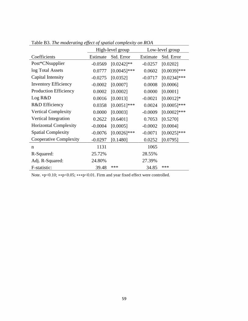
59

Table B3. The moderating effect of spatial complexity on ROA



Post*CNsupplier -0.0569 [0.0242]** -0.0257 [0.0202]

log Total Assets 0.0777 [0.0045]*** 0.0602 [0.0039]***

Capital Intensity -0.0275 [0.0352] -0.0717 [0.0234]***

Inventory Efficiency -0.0002 [0.0007] 0.0008 [0.0006]


Log R&D 0.0016 [0.0013] -0.0021 [0.0012]*

R&D Efficiency 0.0358 [0.0051]*** 0.0024 [0.0005]***

Vertical Complexity 0.0000 [0.0003] -0.0009 [0.0002]***


Horizontal Complexity -0.0004 [0.0005] -0.0002 [0.0004]



n 1131 1065

R-Squared: 25.72% 28.55%

Adj. R-Squared: 24.80% 27.39%

F-statistic: 39.48 *** 34.85 ***


60

Table B4. The moderating effect of cooperative complexity on ROA



Post*CNsupplier -0.0847 [0.0237]*** 0.0125 [0.0216]

log Total Assets 0.0703 [0.0044]*** 0.0710 [0.0043]***

Capital Intensity -0.0216 [0.0352] -0.0828 [0.0253]***


Production Efficiency 0.0001 [0.0001] -0.0001 [0.0003]

Log R&D 0.0001 [0.0013] -0.0015 [0.0012]

R&D Efficiency 0.0424 [0.0075]*** 0.0023 [0.0005]***

Vertical Complexity 0.0000 [0.0002] -0.0011 [0.0002]***


Horizontal Complexity 0.0000 [0.0005] -0.0005 [0.0004]


Cooperative Complexity 0.0273 [0.1127] 0.0364 [0.1072]

n 1366 1095

R-Squared: 22.20% 31.37%

Adj. R-Squared: 21.22% 30.28%

F-statistic: 32.05 *** 41.02 ***


the impact of tariff trade barriers on the operating

Documents