The Impact of Longevity Risk on the Term Structure of the Risk-Return Tradeoff

Emilio Bisetti, Carlo A. Favero, Giacomo Nocera, Claudio Tebaldi* Department of Finance, Università Bocconi

Via Röntgen, 1 - 20136 Milan, Italy * Corresponding author. Tel: +39 02 5836.3638; Fax: +39 02 5836.5920. E-mail addresses: emilio.bisetti@studbocconi.it (Emilio Bisetti), Giacomo.nocera@unibocconi.it (Giacomo Nocera), carlo.favero@unibocconi.it (Carlo A. Favero), claudio.tebaldi@unibocconi.it (Claudio Tebaldi)

The Impact of Longevity Risk on the Term

Structure of the Risk-Return Tradeoff

Preliminary draft: please do not circulate

February 17, 2012

Abstract

The increase in worldwide life expectancy finds a major drawbackin the higher-then-expected liabilities that annuity providers will facein the next years by paying more retirees for a longer period of time.In this paper we investigate the potential of Longevity-Linked Securi-ties as instruments to increase the risk-sharing and diversification oflongevity risk by means of financial markets.

Differently from previous approaches, we explicitly address thisproblem by taking into account the long-term nature of these risks.

In fact, we analyze the modification of the term structure of therisk-return tradeoff as determined by the addition of an ideal longevity-linked security to the set of traditional Stocks, Bonds and T-Bills in-vestment opportunities.

We complement this analysis producing a quantitative estimationof the longevity risk compensation based on annuity markets prices.

1 Introduction

It is a matter of fact that worldwide life expectancy has gone through majorimprovements throughout the past Century, and that these improvementsare still in place. Even if nature has (up to now) posed a limit to hu-man life at around 120 years1, discoveries in the fields of healthcare andmedicine, coupled with higher quality of life, have led to an overall increasein longevity, especially at old ages.

1www.grg.org

1

If in 1967 a US male aged 65 had a life expectancy of 12.99 years, by1987 this value increased to 14.69 and to 17.52 by 2007. Similarly, the total(male and female) life expectancy at birth during the period 1959-1961 was69.9, it was 75.4 during the period 1989-1991 and 77.5 in 2003 (Shrestha[16]). Finally, following the so-called phenomenon of ”rectangularization”(the shift to the right of the frequency of deaths), in 1971 the modal age ofdeath in the US was 79 years, while it was 86 years in 2000 (Canudas-Romo[7]).

Although these data and estimates sound encouraging from our perspec-tive, they represent a major issue for pension funds, insurance companiesand annuity providers in general. Longevity risk is the risk that an annu-itant will live more than forecasted by the annuity provider, such that thecompany will have to pay an annuity for a longer-then-expected period afterher retirement.

Several solutions have been implemented in the past few years in order tohedge longevity risk. Traditional ones encompass reinsurance and increasein premia paid by the insured, while an alternative has been recently discov-ered in the so-called Longevity-linked securities, created in order to transferlongevity risk to the financial markets. The Longevity Bond, in particular,is an asset designed to provide its buyer with a longevity risk hedge thanksto the particular structure of its coupons, which are directly proportional tothe longevity of a reference population and thus mimicking and offsettingthe behavior of the pension annuities’ liabilities.

Recent research has focused on longevity risk, longevity-linked securitiesand their pricing (in particular, see Blake et al. [1], Cairns et al. [3], Fried-berg and Webb [8], Lin and Cox [13] and Menoncin [15]). While standardpricing approaches are based on the hypothesis that the investor’s horizonis short term, i.e. that the risk is measured by instantaneous variance andfrequent trading can fully diversify also those high persistence risk compo-nents which should be the main concern of long horizon investors, this workconsiders the analysis of longevity risk from a different perspective. Takinginspiration from the analysis of the term structure of risk-return trade-off,initiated by Campbell and Viceira [6] and described in section 4, the char-acterization of longevity risks is performed by explicitly accounting for theirlow volatility high persistence features.

The presentation of the results will make clear that the characterization

2

of the whole term strucuture of risks is a necessary step in order to createthe conditions for a transparent and efficient market for the risk sharing oflongevity risk.

The rest of the paper is organized as follows: in section 2 we derivea proxy for the US retirees’ longevity risk during the second half of thepast Century, which we named Longevity Shock. In section 3 we presentand replicate the asset allocation model developed by Campbell and Viceirain [6], which has the advantage of deriving the term structure of the risk-return trade-off of financial assets for different investment horizons. Themodel is used in section 4 to relate Longevity Shocks to financial marketsand interpret the results. Section 5 analyzes the Longevity Risk Premiumin Life Annuities. The last section concludes.

2 Longevity Shocks

We define Longevity Shock as the error between realized and forecastedlongevity of a particular set of US males and females’ cohorts during theperiod 1952-1995. These Shocks are, per se, not an asset nor the returnson a Longevity Bond. The price and the returns of the latter are, in fact,affected by both longevity risk (at the numerator of the equation for theprice of Longevity Bonds as reference rate for their coupons) and by interestrate risk (which determines at which rate the coupons of the Bond shall bediscounted).

Longevity Shocks can be seen as a proxy for what happens at the numer-ator of the Longevity Bond equation, and as the longevity risk embeddedinto a Longevity Bond with a wide and diversified population of US retireesas underlying. We will now describe the derivation of Longevity Shocksstarting from the description of the widely used Lee-Carter model (see Leeand Carter [11]) from which we obtained our forecasts of longevity.

2.1 The Lee-Carter Model

The model in its basic form was developed by Ronald D. Lee and LawrenceR. Carter in 1992 [11], and was further refined by successive studies. Wedecided to focus our analysis on its original version because of its wide useand the ease of comprehension.

3

Model Description The power of the Lee-Carter model lies in the factthat the only relevant variable in forecasting mortality rates is the mortalityfactor, k, unique amongst all ages. The central mortality rate mx,t for age xat time t moves in the Lee-Carter model according to the following equation:

ln[mx,t] = ax + bxkt + εx,t (1)

where ax and bx are age-specific constants and kt is a time-varying mor-tality index. In particular, bx tells us which mortality rates decline rapidlyand which decline slowly in response to a change in the mortality index k.The error term εx,t with mean 0 and variance σ2ε , reflects age-specific influ-ences not captured by the model.

The main problem is how to determine the time-varying mortality indexkt, which is by itself not obervable. The model described in equation 1 can-not, in fact, be specified with ordinary regression methods, as there are noregressors: on the right-hand side of the equation we only find parametersto be estimated (ax and bx) and the unobservable index kt.

The Singolar Value Decomposition method (SVD henceforth), was usedby the authors to obtain a unique solution to the estimation problem2. Inorder to find a unique solution to equation 1, the authors3 first imposed theconstraints that

∑t kt = 0 and

∑x bx = 1. The first normalization implies

that ax is the empirical average of ln[mx,t], and 1 can be rewritten in termsof the mean-centered log-mortality rate as

ln[mx,t] − ln[mx,t] ≡ m̃x,t = bxkt + εx,t

Grouping all the m̃x,t in an unique (X × T ) matrix m̃ (where the columnsare mortality rates at time-t ordered by age groups and the rows are mor-tality rates through time for a specific age-group x), the authors used SVD

2SVD is a technique based on a theorem of linear algebra stating that a (m × n)rectangular matrix M can be broken down into the product of three matrices - an (m×m)orthogonal matrix U , a diagonal (m × n) matrix S, and the transpose of an orthogonal(n × n) matrix V . The SVD of the matrix M will be therefore be given by M = USV ′

where U ′U = I and V ′V = I. The columns of U are orthonormal eigenvectors of AA′ ,the columns of V are orthonormal eigenvectors of A′A, and S is a diagonal matrix whoseelements are the square roots of eigenvalues from U or V in descending order.

3The explicit derivation of bx and kt is not so clear in the original paper [11]. Girosiand King [10] and Giacometti et al. [9] give more detailed explainations on how to obtainthese values.

4

to obtain estimates of bx and kt.

In particular, if m̃ can be decomposed as m̃ = USV ′, b = [b0, b1, . . . , bX ]is represented by the normalized first column of U, u1 = [u0,1, u1,1, . . . , uX,1],such that

b =u1∑X

x=0 ux,1

On the other hand the mortality index vector k = [k1, k2, . . . , kT ] is givenby

k = λ1(X∑x=0

ux,1)ν1

where ν1 = [ν1,1, ν1,2, . . . , ν1,T ]′ is the first column of the V matrix andλ1 is the highest eigenvalue of the matrix S (see Girosi and King [10] andGiacometti et al. [9]) .

The values of mortality rates obtained with this method will not, ingeneral, be equal to the actual number of deaths. The authors hence re-estimated kt in a second step, taking the values of ax and bx as given fromthe first-step SVD estimate and using the actual mortality rates. The newvalues of k were obtained such that, for each year, the actual death rateswould have been equal to the implied ones. This two-step procedure allowsto take into account the population age distribution, providing a very goodfit for 13 of the 19 age groups, where more than 95% of the variance overtime was explained. For seven of these, more than 98% of the variance wasexplained.

The next step after fitting the model was that of making adequate fore-casts for the mortality rates. Thanks to the mortality index k, which isunique amongst all age groups and moves in a quite persistent fashion,making forecasts becomes much easier. The authors found that an adequateARIMA model describing the behaviour of the mortality index k during theperiod 1900-1989 is

kt = kt−1 − 0.365 + 5.24flu+ et (2)

where flu represents a dummy variable for the 1918 influenza epidemic4.

4According to the authors, neglecting this variable would provide substantially un-changed point forecasts and parameters, but a 57% wider confidence interval for the lastforecast of kt in 2065.

5

The R2 of this regression is 99.5%.

The combination of 1 and 2 allows to make forecasts about mortalityrates from which to derive longevity rates and related Longevity Shocks.We will now explain in detail the steps followed.

Forecasting Mortality rates We used the yearly central mortality ratesfor the total US population (males and females) from the Berkeley HumanMortality Database5. The mortality rates refer to age groups 0-110+ forthe period 1933-1995. This is the main difference from [11] as the authorsused age groups of five years, but we will prove the model consistent alsowith single-age datasets. We selected the period 1933-1951 to derive thefitted values of the mortality index kt, and the consequent years 1952-1995to make forecasts on the levels of Longevity Shocks.

Forecasts are made on a year-by-year basis, since Longevity Shocks arecalculated as the unexpected error between the estimates of longevity fromthe previous year and the realized longevity rates. We therefore recoursivelyestimated the parameters ax, bx and the ARIMA model of kt from 1951 to1994 to account for improvements/deteriorations in US longevity during theselected period. This gave us fourty-four estimates for the vectors k, a andb in equation 1 as well as fourty-four estimates for the intercept and theAR(1) parameter in equation 2. Since the data start from 1933, we didn’tneed to take the flu dummy into account.

Table 1 shows the values of ax and bx we obtained for the last estimate,when the fit of the model is made on the largest sample 1933-1994. As wecan see, our results are not radically different from those obtained by Leeand Carter, also taking into account that the authors used five-years agegroups, while we made forecasts for age groups of one year.

Figure 1 plots the mortality index kt relative to the 1933-1994 sample.The index decreases roughly linearly with time and is in line with the k esti-mated by Lee and Carter. We should pay particular attention in comparingthis Figure to the one of their paper, however, since the index is particu-larly subject to data specification. Results are in this sense closer to thoseobtained by Li and Chan [12] for the US population.

5http://www.mortality.org/cgi-bin/hmd/country.php?cntr=USA&level=1

6

Finally, modelling the series of kt estimated through the whole 1933-1994sample we obtained the following ARIMA process

kt = −0.6034 + 0.9763kt−1 + et

which is very similar to equation 2, and then estimated mortality ratesaccordingly.

2.2 Longevity Shocks: definition and derivation

Once obtained Lee-Carter forecasts of mortality rates, the next step was tofind a suitable definition of Longevity Shock. This definition must respondto the following criteria:

• It should cover unexpected improvements/deteriorations in longevity,defined as the realized differences between expected and realized longevity.

• It should be as comprehensive as possbile, reflecting the behaviour ofthe whole retired US population (males and females aged from 65-110+) during the period 1952-1995.

• It should reflect the longevity risk borne by an annuity provider witha diversified portfolio of US annuitants.

As for the first point, for each year from 1952 to 1995 we developedmortality forecasts based on the Lee-Carter model for the whole retiredpopulation 65-110+. In our analysis we will consider age gropus from 65onwards because this is the typical retirement age, starting from which in-surance companies and pension funds start paying annuities. We assume infact that if an unexpected increase in longevity is registered in a particularyear, the annuity provider will be able to adjust the premia for those whoare still working. The risk is therefore concentrated to the part of the pop-ulation which is retired, because here no premium adjustment can be made.Anyway, we should keep in mind that particularly for old ages (higher than90-94 years), the estimates are quite noisy due to the high variability ofmortality rates6.The time-t expected longevity Et(Lx,t+1) for each of the 46

6If for example there were only ten people alive at the age of 109 at the beginningof 1976 in the US and of these ten people only five surivived to the end of 1976, thenm(109, 1976) = 50%. Similarly, if there were only ten people alive at the age of 109 atthe beginning of 1977 and of these ten people seven surivived to the end of 1977, thenm(109, 1977) = 70%. These volatile changes in mortality rates from one year to anothermakes it very hard to make good forecasts for very high ages.

7

age groups was then given by

Et(Lx,t+1) = (1 − Et(mx,t+1))

where Et(mx,t+1) is the time-t expectation of the central mortality rate ofage group x for the following period t+ 1.

The realized longevity rate for age group x at time t + 1 was similarlygiven by

Lx,t+1 = (1 −mx,t+1)

and the difference between the realized longevity rate and the expectedone is our age-specific t+ 1 Longevity Shock, ηx,t+1

7.

As for the second and the third points, the problem was determiningan unique measure of the Longevity Shock for each year instead of fourty-six shocks corresponding to each age group. In order to do so, we createda vector of weights representing a diversified portfolio of annuitants of anhypothetical US pension fund. We considered the US 65-110+ years-oldpopulation distribution for the years 1951-1994, whose data we downloadedfrom the Berkeley Human Mortality Database. In this portfolio the (chang-ing) weight assigned to each Longevity Shock in year t + 1 would be equalto

ωx+1,t+1 =popx,t∑110

x=65 popx,t

where ωx+1,t+1 is the weight assigned to ηx+,t+1, popx,t is the total US pop-ulation aged x at time t and

∑110x=65 popx,t corresponds to the sum of total

retired US population in year t.

We assume that forecasts of mortality rates are made at the end of theyear previous to that of the realization of longevity. Population weightsare therefore chosen such that the portfolio of insured that will experiencea particular mortality rate in year t + 1 is the one that the hypotheticalannuity provider had on its book at the end of t.

The portfolio both represents the highest possible degree of diversifica-tion, since it takes into account the whole retired population, and gives less

7Notice that this definition does not take into account Cumulative Survival Rates, asShocks are based on forecasts made each year relatively to the following one, only. Thisavoids both the problem of making long-term forecasts of mortality and is consistent withthe periodic (yearly) adjustments to mortality projections made by actuaries.

8

weight to more volatile forecasts corresponding to high-age groups. More-over, its weights take into account periodic changes in the balances of thepopulation structure, making it appealing also in terms of interpretation.Figure 2 plots Longevity Shocks for the period considered. As we cansee, this ”Demographic” specification provides us with constantly positiveShocks reflecting the overall age-weighted unexpected improvement in USlongevity in the period 1952-1995.

3 Term Structure of Risk-Return Tradeoff

This section is devoted to the description and implementation of a modelwhich allows to find different values of expected returns, variances and cor-relations of a set of variables depending on a selected investment horizon.The original model is the simple yet powerful one developed by Campbelland Viceira [6].

3.1 The Theoretical Framework

The authors propose a very simple yet effective Vector Auto-Regressivemodel of order one (from now on, VAR(1)), which finds a wide range ofapplications in macroeconomic theory. The basic prediction of this model isthat every component of a vector of variables depends on the n-lag (in thiscase, the lag length is one) values of the same vector plus an error term.

The variables are excess returns on Stocks and Bonds, real returns onT-Bills plus three factors which are commonly recognized as good returns’predictors. These are the short-term interest rate, the Dividend Price ratioand the Yield Spread between long-term and short term Bonds. Furtherdetails on the variables’ specifications are given in the next subsection. Informulas, we have that each one of the six variables can be represented bythe following process

rj,t = φj,0 +6∑i=1

φj,iri,t−1 + εj,t fori = 1, 2, . . . , j, . . . , 6

or alternatively, in vector notation,

Rt = Φ0 + Φ1Rt−1 + εt (3)

9

where Rt is a (6 × 1) column vector of the variables at time t, Φ0 is a(6 × 1) column vector of the intercepts of the model, Φ1 is a (6 × 6) matrixof coefficients assigned to the one-period lagged variables and εt is a (6× 1)vector of error estimates.

This easily implementable model allows us both to take into accountmutual relationships between the six variables and to understand how theseare related in a context with different investment horizons. The conditionalexpectations and variances which we derive from this model are in fact ex-tremely different from the unconditional ones, which are simply the historicalmean and variances of the sample, and this is where the Campbell-Viceiramodel proves most useful. The investor who uses the VAR(1) model in or-der to make forecasts about the expected risk-return structure will differin many ways from the investor who uses unconditional expectations andvariances (see Campbell and Viceira [6]):

• First of all, the former will have a different return expectation on eachperiod t (based on the t−1 values of both the state variables and assets’returns) if compared to the constant unconditional expectations of thelatter.

• Secondly, the VAR(1) investor will have a different and dynamicallychanging expectation for the variance structure, which will also de-crease as part of the variability in the forecasts is explained by themodel. The risk will be embedded in the error term ε which repre-sents the part of return which the model is not able to predict.

• Thirdly, the risk-return profile of each asset will differ depending onthe holding period. While in fact for the ”unconditional” investorthe per-period return of an asset and its relative risk are constantthrough time, this is not true for the VAR(1) investor, who will beable to allocate assets differently according to the per-period forecastsof annualized expected values, variances and correlations of returns.

3.2 Replicating the Campbell-Viceira model

As explained in section 2, we derived Longevity Shocks with annual fre-quency. Since adapting this series to the quarterly model originally used in[6] would have been both hardly feasible (lack of longevity data for frequen-cies higher than yearly) and meaningless (for example, because there aresome months of the year which experience particularly high death rates),

10

we decided to adapt the Campbell-Viceira model to the annual LongevityShocks ranging from 1952 to 1995, inclusive.

The original data refer to Campbell et al. [4] and cover the period 1890-1995. In particular, the six time series are built as follows:

• Short-term ex-post real rate: return on 6-month commercial paperbought in January and rolled over July, minus the Producer PriceIndex (PPI).

• Excess Return on Stocks: log return on the S&P 500 Stocks, fromwhich the short-term interest rate has been subtracted.

• Excess Return on Bonds: returns have been obtained using the log-linear approximation described in section 10 of Campbell, Lo andMacKinlay [5]

rn,t+1 = Dn,tyn,t − (Dn,t − 1)yn−1,t+1

where n is the Bond maturity, the Bond yield is Yn,t, the log Bondyield is yn,t = (1 + Yn,t) and Dn,t is the Bond duration, calculated attime t as

Dn,t ≈1 − (1 + Yn,t)

−n

1 − (1 + Yn,t)−1

with n set to 20 years and yn−1,t+1 approximated by yn,t+1.

• Nominal T-Bill rate: return on 6-month commercial paper bought inJanuary and rolled over July.

• Log Dividend Price ratio: natural logarithm of the S&P 500 dividendseries minus the logarithm of the S&P 500 price series.

• Yield Spread: difference between the log yield of the long Bond andthe short yield on the commercial paper.

VAR(1) estimation Table 2 shows the results of our VAR(1) estimationfor the yearly sample (period 1952-1995), coupled with its correspondingt-statistics. The bottom part of the Table reports correlations of the inno-vations of the VAR(1).

Starting from the T-Bill equation in the upper parts of Table 2, we cansee that the coefficient attached to the lagged real T-Bill rate is positive

11

and significant, while that on the Yield Spread coefficient is negative. Thismeans that a positive shock to the real T-Bill rate today predicts a higherT-Bill rate for the next period and conversely that a positive shock to theYield Spread today predicts a lower T-Bill rate for the next period. Theforecasting power of the equation is pretty high, 59.4%.

The second row shows us how it is difficult to predict Stocks’returns,as the forecasting power of each of the six lagged explanatory variables isvery poor. All the coefficients are not statistically different from zero andthe predictive equation shows a small R2 of 7.6%. Excess returns on theBond are explained by the lagged values of real T-Bill returns, Yield Spreadand excess Bond returns (the latter two with negative coefficients, the firstone with positive coefficient), and the predictive power of the equation isvery high in this case, with an R2 of 58.9%. We should, however, keep inmind that the results could reflect approximation error in constructing ex-cess Bond returns.

The last three rows show coefficients and relative t-statistics for the statevariables. All of the three show high persistence, and the Dividend Priceratio moves as an AR(1) process. The nominal T-Bill yield and the YieldSpread are, instead, also explained by the lagged real T-Bill rate and theYield Spread by the lagged nominal T-Bill rate.

The bottom part of Table 2 shows the standard deviations (on the maindiagonal) and the cross-correlations (off the main diagonal) of the regressionresiduals. As we can see, the most relevant correlations are those betweenthe Dividend Price ratio and excess Stock returns, excess Bond returns andthe nominal T-Bill rate and finally the nominal T-Bill rate and the YieldSpread. The variable which shows the highest variability is the excess Stockreturn, followed by the Dividend Price ratio. The results are overall verysatisfactory, as they resemble those obtained by Campbell, Chan and Viceirain [4].

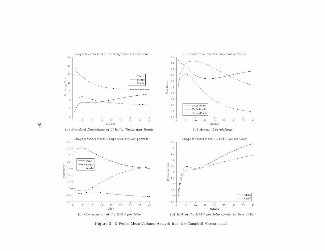
K-period Mean-Variance Analysis Looking at Figures 3a and 3b wecan see how the basic intuition underlying the Campbell-Viceira model holdstrue. Both per-period annualized standard deviations and per-period cor-relations of assets’ returns show different patterns for different forecastinghorizons. The maximum horizon has been chosen to be equal to 40 years,because this duration is consistent with that of a longevity-linked security

12

(ideally, a Longevity Bond).

Starting from Figure 3a, we can notice that the standard deviation ofStocks decreases from a high of 14% to a low of 9% at long horizons, drivenby the Dividend Price ratio. This variable is in fact highly negatively corre-lated with the current level of Stocks’ returns, but at the same time forecastsa high value of Stock returns for the next period, causing their mean rever-sion and decrease in variance.

A similar behaviour is followed by the Bonds’ standard deviations. Inthis case the initial increase in risk is due to the mean-averting effect of theYield Spread. This variable is positively correlated with the current valueof the Bond return, and at the same time its lag-one coefficient is positivein the equation of excess Bond returns. This effect causes mean aversion,whose effect is higher at short term horizons of 5 to 10 years.

The T-Bill is conversely charachterized by mean-aversion, led by its greatpersistence. This takes the value of its standard deviation from a low of 3%to a maximum of 8% at an investment horizon of 40 years. We can clearlynotice how, for an investment horizon of 15 years onwards, the risk of aT-Bill is even higher than that of the Bond. This is due to the fact thata T-Bill held for short-term investment horizons equal to their natural ma-turity carry only a small inflation risk. On the other hand, a long-terminvestment in T-Bills carries a significant reinvestment risk, which radicallychanges their risk-return profile.

Figure 3b plots the correlations between the three assets for investmenthorizons up to 40 years. First of all, the correlation structure betweenStocks and Bonds follows an initial increase mainly driven by the relevanceof the nominal T-Bill yield at intermediate horizons (around 5-15 years). Apositive shock to y corresponds in fact to an immediate decrease in Bond’sreturns (as the correlation between the two variables is highly negative), butalso predicts a low return on Stocks. This effect takes some time to be fullyincorporated into the correlations between Stocks and Bonds, such that thehighest values of correlations are realized at horizons of around 10 years. Atlonger investment horizons, a shock to the more persitent Dividend Priceratio predicts shocks of opposite sign to Bonds and Stocks, lowering backthe correlation to around zero.

Secondly, T-Bills and Bonds are affected in the same way by a shock to

13

the nominal T-Bill yield. This effect corresponds to an immediate increasein the correlation between the two variables for horizons up to 5 years, fol-lowed by a decrease explained by the opposite signs of the Dividend Priceratio in predicting Bonds and T-Bills’ returns.

Finally, the initial drop in correlations between Stocks and T-Bills isagain due to the opposite signs of the lagged nominal T-Bill coefficient inexplaining the two variables. This effect is, for forecasting horizons higherthan 15 years, offset by the fact that the coefficients on the Dividend Priceratio have the same sign in the predictive equations of T-Bills and Stocks.

Global Minimum Variance Portfolio The fact that an investment ineither T-Bills, Stocks or Bonds can have a different risk-return profile fordifferent investment horizons has important implications for optimal port-folio allocation. Traditional mean-variance asset allocation (see Markowitz,[14]) focuses on risk at horizons between one month and one year, and whenthe term structure of risk is flat this model can also hold true for asset al-locations with longer horizons. Nonetheless, as we just showed, the termstructure of the risk-return profile of different assets is far from being con-stant.

In order to make this point clear we will now consider a particular port-folio, the Global Minimum Variance (GMV henceforth) portfolio. This isrepresented by the leftmost point in the mean-variance diagram, and hasthe interesting property of always having the smallest variance amongst allthe efficient investments. When a riskless asset is available, this portfoliowill be 100% invested in the riskless asset. Otherwise its composition willbe made by the (three in our case) assets available.

Figure 3c shows the composition of the GMV portfolio. The relativeweight of the T-Bill decreases from an high of around 120% at investmenthorizons of 5 years to a low of 50% at horizons of 40 years. Correspondingly,the relative weight associated to the Bond is slightly higher than that of theT-Bill (around 60%), and the weight assigned to Stocks, in relation to theirhigh risk, is always slightly negative (i.e. the GMV investor will sell Stocksshort for every investment horizon).

Figure 3d plots instead the annualized standard deviation of the realreturn on the GMV portfolio, together with the annualized percentage stan-

14

dard deviation of the real return on the T-Bill. As we can see, the risk ofthe GMV portfolio is always lower than that of the T-Bill, in contradictionto traditional financial theory according to which the T-Bill is ”risk-free”.This effect is even clearer for long investment horizons, where the spreadbetween the two standard deviations is more than 1.5% (even if around 60%of the overall portfolio is invested in Bonds, 60% in T-Bills and Stocks aresold short for a percentage equal to 20% of the portfolio).

4 The Term Structure of Longevity Risk

This section describes the procedure we used to include the Longevity Shocksderived in section 2 inside a VAR(1) system. Its aim is that of analyzingwhether the unexpected increase/decrease in overall US longevity duringthe years 1952-1995 has been related to the financial variables described insection 3 and, if so, how.

The results are, on one hand, interpreted in a risk perpspective, an-alyzing how variances and correlations of the financial and demographicvariables both vary depending on the investment horizon and can be af-fected by longevity risk. On the other hand, the risk-return profile of thevariables is analyzed in terms of optimal asset allocation, interpreting thelong-term longevity risk-return term structure in an optimal asset allocationperspective. As in section 3, in fact, we derive the composition of the GMVportfolio in presence of Longevity Shocks and draw conclusions about itsrelative composition.

4.1 VAR(1) estimation

Table 3 shows the results of the VAR(1) estimate including Longevity Shocks,which we can compare to those in Table 2. As for the upper part of Table 3,no major changes take place in the coefficients attached to the six financialvariables with respect to Table 2. For those variables whose explanatorypower is significantly different from zero, in particular, the signs are thesame as in Table 2.

The overall fit of the model increases. In order to make meaningful com-parisons between the two versions of the VAR(1), we report the adjustedR2 for both of them. Adding Longevity Shocks increases the adjusted R2

of the model for all the equations but the one relative to the Yield Spread,

15

and therefore seems meaningful.

The coefficients attahced to the Longevity Shocks are always significantand their sign is negative in the predictive equations of the three financialassets. A positive Longevity Shock today would, according to our resultspredict lower returns on T-Bills, Bonds and Stocks. The fourth row showsthe coefficients of the equation of Longevity Shocks. The variable is quitepersistent and lagged Bond returns have explanatory power over it. Theoverall fit of the equation is quite high (the R2 is in this case 64.6%).

The last three rows represent the three state variables. In this case,too, no major changes occur when Longevity Shocks are added to the sys-tem. The variables still show very high persistence and the coefficient of thelagged real T-Bill equation is positive both in the equation for the nominalT-Bill and in the one of the Yield Spread. The lagged nominal T-Bill rateacquires explanatory power in the Yield Spread equation, while interestinglyLongevity Shocks receive a positive and significant weight in forecasting theDividend Price ratio.

Comparing the bottom parts of Tables 3 and 2, we can immediatelynotice a general drop in standard deviations of the regression residualswhen adding Longevity Shocks to the VAR(1). This is not a surprise, asadding new regressors decreases the residuals’ variance8. However, the cor-relation structure of the residuals looks pretty similar to the one withoutLongevity Shocks. The residuals’ correlations between T-Bills, Bonds andStocks slightly decrease in all the three cases as Longevity Shocks show thesame (negative) sign in forecasting all of them, thus decreasing their resid-uals’ common variation.

Longevity Shocks are negatively correlated with T-Bill rates, excessStock returns and nominal T-Bill rates. They are instead positively cor-related with excess Bond returns, the Dividend Price ratio and the YieldSpread. Noticeably, the Shocks show their highest levels of correlation withthe Dividend Price ratio (the variable whose effects are the most relevant atmedium/long horizons) and the lowest with the short-term real T-Bill. Thisissue will be investigated further in the next subsection, where the correla-tion structures are analyzed in relation to different investment horizons.

8This is the reason why we chose to use the adjusted R2 rather than the simple R2 toexplain the overall fit of the model

16

Which conclusions can we derive from our results on the relationshipbetween financial markets and longevity risk?

• Longevity Shocks display an extremely low variance, much lower forexample than that of a T-Bill and also lower than that of the threestate variables.

• An unexpected increase in longevity today forecasts a positive LongevityShock for tomorrow. This reflects the overall improvement in thelongevity profile of the US population which is not accounted for bythe Lee-Carter model.

• The current value of Longevity Shocks is negatively correlated withStocks and T-Bills’ returns and positively correlated with excess Bondreturns. This not only confirms the widespread opinion according towhich investing in longevity risk offers an attractive diversification op-portunity, but also strengthens it as, instead, the correlation betweenfinancial markets and longevity risk is negative.

• At the same time, positive Longevity Shocks predict low returns onStocks, Bonds at T-Bills, and high Dividend Price ratios.

• Adding Longevity Shocks to the original VAR(1) with annual dataleads to an overall improvement of the predictive power of the equa-tion, measured by its adjusted R2.

4.2 K-period analysis of risk and GMV portfolio

This section is devoted to the analysis of variances and correlations of thesix original variables and Longevity Shocks. The main point is trying tounderstand wheather unexpected improvements in Longevity are correlatedwith financial markets in a K-period investment horizon framework, and, ifso, the extent of these correlations.

Longevity Shocks and Financial Variables Looking at Figure 4a, re-porting the standard deviations of T-Bills, Stocks, Bonds and LongevityShocks for different horizons, we can make some immediate comparisonswith its counterpart Figure 3a.

First of all, Longevity Shocks show the lowest risk for all the investmenthorizons. Their standard deviations pass from a low of 0.155% to a high of

17

around 0.5% at a 40 years’ horizons. This increase (which, despite its lowabsolute value, more than triplicates the risk of the variable) is driven bythe high persistence of Longevity Shocks and by the mean-averting effect ofthe Dividend Price ratio. On one hand, in fact, the Dividend Price ratiodisplays positive correlation with Longevity Shocks. On the other hand, apositve shock in the Dividend Price ratio forecasts a high level of LongevityShock for the next period. The combined effect causes mean-aversion.

As for the other variables’ risk, we can notice an overall decrease in thelevels of standard deviation, explained in the previous section with the in-creased number of regressors. Their shape for different investment horizonsis, however, almost left unchanged.

The standard deviation of Stocks’ returns does not change, except forthe fact that the mean-averting effect of the Dividend Price ratio is slightlymore pronounced in this case (its coefficient passes from 0.08 to 0.36 in theequation of Stocks’ returns). Similar conclusions can be drawn for Bonds,whose risk profile is identical to the one displayed in Figure 3a.

As for T-Bills’ standard deviation, we can notice a small decrease inthe curve at very long horizons (around 20 years) corresponding to a re-duced mean aversion effect. This could again be imputed both to the highermean-reverting power of the Dividend Price ratio when Longevity Shocksare added to the VAR(1) system but also to the lower persistence of the realT-Bill’s return itself.

Figure 4b shows correlations between the three financial assets’ returns(Bonds, T-Bills and Stocks) and Longevity Shocks. Starting from the initialvalues in Table 3, the correlation between Bonds and Longevity almost dropsto a minimum of -60% at an horizon of seven years. This is justified by thepersistence of Longevity Shocks and by their explanatory power on excessBond returns. A positive Longevity Shock today, in fact, translates into apositive Bond return today. At the same time, a positive Longevity Shockforecasts a negative excess Bond return and a positive Longevity Shock forthe next period. These counterbalancing effects imply that the decreasein correlations between Bonds and Longevity Shocks will take more timeto reach its full effect relatively, for example, to the correlations betweenStocks, T-Bills and Longevity.

After this initial drop, however, more persistent variables such as the

18

Dividend Price ratio, the nominal T-Bill rate and the Yield Spread takeback the Bonds/Longevity correlation to around -30% as all have the samesigns in the predictive equations of Longevity Shocks and Bonds.

Similar conclusions can be drawn for Stocks and Longevity. The nega-tive correlation is, on one hand, driven by the opposite signs of the laggedLongevity Shocks’ coefficients in the equations of excess Stock returns andin that of Longevity Shocks. On the other hand, it is further strengthenedby the negative correlation between the two variables. This means that apositive Longevity Shock implies a negative excess Stock return today, andforecasts a negative excess return on Stocks and a positive Longevity Shockfor the next period. This effect therefore takes a very short time to be fullyincorporated in the Stocks/Longevity correlations (in particular, the min-imum is reached around a 5-years’ horizon, and corresponds to a value of-55%).

What we just described also holds true for T-Bills and Longevity. Themedium-term reversion effect is even more pronounced here and the low-est levels of correlation are displayed around 3-years’ investment horizon.The influence of Longevity Shocks leaves soon room to the more persistentDividend Price ratio and nominal T-Bill yield, whose effects lead the finalcorrelations at a 40-years horizon to around 20%.

Our results confirm the opinion according to which longevity risk is aninteresting diversification opportunity with respect to Stocks (at any invest-ment horizon), and with respect to T-Bills (at an horizon from 0 to 15 years).The long-term longevity-risk return profile will, however, radically changedepending on the investment horizon and hits shall be accounted for as theinvestment horizon of such an investment should be a very long one.

What happens to the term structure of correlations of financial variables?Comparing Figure 4c and Figure 3b, we can clearly notice that the shapeof the curves does not change much when adding Longevity Shocks intothe VAR system. The only relevant difference lies in Stocks and LongevityShocks for an investment horizon between 5 and 15 years. As we can see,in fact, the correlation does no more show the drop which we imputed tothe nominal T-Bill rate’s coefficient in Figure 3b. Even if the coefficientsattached to the lagged nominal T-Bill rate still show opposite signs in fore-casting Stocks and Bonds, their effect is partially offset by the fact that apositive Longevity Shock forecasts negative real T-Bill and Stocks’ returns.

19

The fact that Longevity Shocks have a significant explanatory power affect-ing T-Bills and Stocks is also clear if we compare Figures 4b and 3b. Wecan clearly see in 4b that starting from an horizon of around five years,the correlations of T-Bills and Stocks with Longevity are increasing. At thesame time, the correlation between Stocks and T-Bills in Figure 4c decreasesas driven by the nominal T-Bill, but less than in 3b. This is precisely dueto the effect of the common variation of Stocks and T-Bills with LongevityShocks.

K-period GMV with Longevity Shocks Figure 4d shows the compo-sition of the GMV portfolio when Longevity Shocks are taken into account.As we have already noticed, Longevity Shocks always show the lowest vari-ance in the set of variables, and therefore receive a weight of around 100%.Moreover, given the decrease in the Bond’s standard deviations (see Figure4a), from ten years onwards Bonds receive slightly higher weights, (around0.5%). This is also given by the high negative correlation between LongevityShocks and Bonds, which precisely at an horizon of around 10 years displaysits lowest values (around -60%, see Figure 4b). Stocks almost always receivezero-weights, given the high levels of their variance. From 10 years’ horizons,the weight assigned to T-Bills is even negative, meaning that the investor willborrow money to finance her low-risk investment in Longevity and Bonds.

Our results tell us that an annuity provider interested into hedging itslongevity exposure by means of longevity-linked securities will also be able tohave an effective diversification opportunity for its traditional asset classes’risk given the extremely low variance of longevity risk and its negative cor-relation with financial markets.

5 Longevity Risk Premia in Life Annuities

This section is devoted to the analysis of the risk premia for Longevity Riskembedded into Life Annuities. Its aim is that of finding out whether LifeAnnuities’ premia during the second half of the twentieth Century includeda premium for longevity risk (under our definition of Longevity Shock). Inorder to do so, we run regressions on the log returns of Life Annuities Premiaduring the period 1952-2007 and tried to relate them with different defini-tions of Longevity Shocks and other explanatory variables.

The data are relative to the premia for immediate 1$ monthly life annu-

20

ities in the US for 65-year-old males. For each year, they are represented bythe mean value of a sample of prices applied by different US companies indifferent months. We also added the maximum and the minimum values ofthese prices in order to have a measure of their dispersion when performingregressions. The series ranges from 1952 to 2007 and decreases roughly con-stantly from 1952 to 1988. Since a lot of variability is present in prices from1988 to 2007, excluding this period to match it with the Campbell-Viceiracontrol sample of section 3 would have represented a problem in terms of in-terpretation of the results after more than ten years. We therefore decidedto increase the range of Longevity Shocks up to 2007. The data are thesame we used in section 2, downloaded from the Berkeley Human MortalityDatabase.

Moreover, since a relevant component of Life Annuities is related to thebehaviour of interest rates (according to Brown et al. [2] ”the annuity pre-mium has fallen continuously since the late 1950s as the general level ofinterest rates rose”), we decided to take also their effect into account in thepredictive regression of the returns on premia. Unfortunately the data rel-ative to the Campbell-Viceira model do not include the period 1996-2007,and therefore we used another specification for the short-term interest rates,using the annualized 3-months T-Bill rates data we downloaded from theFederal Reserve Bank of St.Louis’ website9.

Table 4 shows our results. The upper part of the Table is dedicatedto the regression where the dependent variable is the end-of-year t − 1 logreturn on the mean annuity premium and the independent variables are theT-Bill rate and Longevity Shocks with no lag, one year lag and two yearslag (identified by the letter k). Since annuity premia are referred to themales-only US retired population and our original definition of LongevityShocks is relative to the whole (males and females) population, we specifiedLongevity Shock based on the US male population, only10.

Our results are satisfactory. The coefficients attached to the T-Bill rateare almost always significant, confirming Brown et al. [2] in the negativecorrelation between interest rates and annuity prices. What is more in-teresting for our analysis is, however, the reaction of annuity premia to a

9http://research.stlouisfed.org/fred2/series/TB3MS?cid=11610The data have the same source and the same reference period as the Longevity Shocks

relative to the total population.

21

Longevity Shock. As we can see, the coefficients attached to the Shocks arealways positive. The middle and the bottom part of the Table, which showthe results of the regressions carried out with the minimum and maximumvalues of the premia as dependent variables, give us a measure of disper-sion confirming this. A Longevity Shock, according to our results, carriesa positive premium as the unexpected increase in longevity is reflected intoa higher premium paid by the insured. Moreover, using k-lagged LongevityShocks tells us when their effect is included into annuity premia.

As we can see, the coefficient attached to the Longevity Shock, γ, gainsmore significance, the higher the value of k. The values of R2, too, increasewith k. They pass from 8.19% to 12.92% and from 16.13% to 21.05% whenthe mean and minimum prema, respectively, are used11.

A Longevity Shock this year is, according to our results, not immediatelyincluded into the premium: even if the coefficients have the right sign in theequation with k = 0, they are not statistically significant. Longevity Shocksare, instead, reflected into premia one to two years after they have occurred.Considering ∆prmean and ∆prmin, the premia attached to longevity riskrange from 6.3169 to 8.4930. Moreover, all four coefficients are statisticallysignificant at a 95% confidence level.

This means that if the population demographic structure remains un-changed from t − 1 and t and an unexpected 1% increase in longevity isregistered during year t− 1 then, correcting for the short-term interest rate,annuity premia returns will be adjusted upwards by around 7% at time t.Similarly, if the population demographic structure remains unchanged fromt− 2 and t and an unexpected 1% increase in longevity is registered duringyear t− 2, annuity premia returns will increase by around 8% at time t.

6 Conclusions

6.1 Final Remarks

Section 4 showed our results regarding the dynamic relationships betweenunexpected changes in the US longevity during the years 1952-1995 and typi-

11Intuitively, prmin should be the least affected by firm-specific charges and size, asusually the more diversified and big the annuity provider, the higher the economies ofscale and the lower the premia charged to the insured. The increase/decrease in the pricesshould then best reflect interest rate and longevity risk.

22

cally financial variables such as Stocks, Bonds and T-Bills’ returns. This un-expected improvements/deteriorations in longevity, called Longevity Shocks,have been derived in section 3 as the retired-population-weighted differencebetween observed longevity and its Lee-Carter estimate.

The common opinion according to which a purely demographic variablesuch as longevity is not related to financial markets does not hold true ac-cording to our results. Longevity Shocks display in fact negative correlationswith real T-Bill and excess Stock returns and positive correlation with theDividend Price ratio during the period considered.

Moreover, the level of the correlation between Longevity Shocks andfinancial markets radically changes across different investment horizons inthe Campbell-Viceira model, and this could be of foremost importance foran annuity provider interested into hedging its longevity exposure with aLongevity Bond12. As we explained in section 2, in fact, the ideal invest-ment strategy for such a security would be a buy-and-hold one, but thiscontrasts with the fact that the longevity-driven coupons of the bond arerevised annually. The analysis carried out in section 4 was therefore aimedat finding the long-term longevity risk-return trade-off profile for a buy-sellstrategy in Longevity Bonds in relation to other investment opportunities.

A diversified portfolio of Stocks would, for instance, display negativecorrelation with longevity for investments horizons from one to forty years,but the level of this correlation radically changes according to the periodconsidered, translating in different optimal asset allocation weights.

The effect is more pronounced for Bonds and T-Bills. As for the former,the initially positive correlation between Bonds and longevity rapidly decaysbelow zero for every investment horizon from 2 to 40 years. If an annuityprovider decides to buy a Longevity Bond today in order to hedge her ex-posure, she will have to take into account that long-term interest rates arenegatively correlated with longevity risk.

As for the latter, the results are even more interesting. If the T-Billcould be considered an effective hedge of longevity risk up to 15 years, thiswould not hold true for longer horizons. The correlation between short-term

12The reader should keep in mind that Longevity Shocks do not represent per se anasset, but a proxy of the longevity risk embedded into a Longevity Bond.

23

interest rates and longevity turns in fact from being negative to positive foran investment horizon of 15 years, changing the optimal asset allocationstructure.

These results obviously depend on our particular specification of themodel used to forecast mortality rates13, but they clearly show that a non-financial variable such as longevity can have an impact on financial ones.

References

[1] D. Blake, A. J. Cairns, and K. Dowd. Living with mortality: longevitybonds and other mortality-linked securities. Pensions Institute Dis-cussion Paper PI-0601, 2006. The Pensions Institute, Cass BusinessSchool, London.

[2] J. R. Brown, O. S. Mitchell, J. M. Poterba, and M. J. Warshawsky. TheRole of Annuity Markets in Financing Retirement. The MIT Press,Cambridge, MA, 2001.

[3] A. J. Cairns, D. Blake, P. Dawson, and K. Dowd. Pricing risk onlongevity bonds. Pensions Institute Discussion Paper PI-0508, 2005.The Pensions Institute, Cass Business School, London.

[4] J. Y. Campbell, Y. L. Chan, and L. M. Viceira. A multivariate modelof strategic asset allocation. Journal of Financial Economics, 67:41–80,2003.

[5] J. Y. Campbell, A. W. Lo, and A. C. MacKinley. The Econometrics ofFinancial Markets. Princeton University Press, Princeton, NJ, 1997.

[6] J. Y. Campbell and L. M. Viceira. The term structure of the risk-returntradeoff. Financial Analysts Journal, 61(1), 2005.

[7] V. Canudas-Romo. The modal age at death and the shifting mortalityhypothesis. Demographic Research, 19(30):1179–1204, 2008.

[8] L. Friedberg and A. Webb. Life is cheap:using mortality bonds to hedgeaggregate mortality risk. NBER Working Paper 11984, 2005. NationalBureau of Economic Research, Cambridge, MA.

13The Lee-Carter model is the most widely used by practitioners, so our estimates oflongevity can be really similar to that of the industry

24

[9] R. Giacometti, M. Bertocchi, S. T. Rachev, and F. J. Fabbozzi. A com-parison of the Lee-Carter model and AR-ARCH model for forecastingmortality rates. Working paper, 2010.

[10] F. Girosi and G. King. Understanding the Lee-Carter mortality fore-casting method. Working paper, 2007.

[11] R. D. Lee and L. R. Carter. Modeling and forecasting U.S. mortality.Journal of the American Statistical Association, 87(419):659–671, 1992.

[12] S. H. Li and W. S. Chan. The Lee-Carter model for forecasting mor-tality, revisited. North American Actuarial Journal, 11:68–89, 2007.

[13] Y. Lin and S. H. Cox. Securitization of mortality risks in life annuities.Journal of Risk and Insurance, 72(2):227–252, 2005.

[14] H. Markowitz. Portfolio selection. Journal of Finance, 7:77–91, 1952.

[15] F. Menoncin. The role of longevity bonds in optimal portfolios. WorkingPaper, 2005.

[16] L. B. Shrestha. Life expectancy in the united states. Technical report,CRS Report for Congress, 2006.

25

7 Figures and Tables

Selected Ages ax bx

65 -3.7539 0.0069370 -3.3669 0.0069675 -2.9288 0.0073080 -2.5084 0.0074585 -2.0603 0.0061990 -1.6428 0.0053295 -1.2968 0.00199100 -1.10568 -0.00227105 -0.96403 0.00026

Table 1: Fitted Values of ax and bx at selected ages from own estimates 1933-1994 (SVD)

Figure 1: Mortality Index kt as from own estimates (1933-1995)

26

Figure 2: Longevity Shocks for total US population, years 1952-1995

27

VAR(1) - Matrix Φ1 - Yearly Sample 1952-1995

rtbt xrt xbt yt (d− p)t sprt R2 adjR2

(t) (t) (t) (t) (t) (t)rtbt+1 0.695 -0.044 -0.044 0.441 0.006 -0.872 0.594 0.524

(4.070) (-1.142) (-0.726) (1.966) (0.182) (-2.054)xrt+1 0.633 -0.252 -0.111 -0.762 0.080 -0.045 0.076 -0.082

(0.902) (-1.495) (-0.331) (-0.580) (0.499) (-0.024)xbt+1 0.610 0.028 -0.444 0.243 -0.052 4.212 0.589 0.519

(2.675) (0.410) (-2.848) (0.483) (-1.148) (5.635)yt+1 -0.204 0.014 0.055 0.842 0.014 0.061 0.767 0.727

(-3.459) (0.794) (1.884) (8.832) (1.551) (0.393)(d− p)t+1 -0.847 -0.099 0.383 -0.203 0.992 -0.683 0.758 0.717

(-1.667) (-0.627) (1.292) (-0.181) (6.925) (-0.392)sprt+1 0.130 -0.018 -0.002 0.147 -0.010 0.563 0.616 0.550

(3.104) (-1.362) (-0.118) (2.301) (-1.444) (4.936)

Cross-Correlations of Residualsrtb xr xb y (d− p) spr

rtb 3.199 0.453 0.003 -0.160 -0.438 0.202xr - 14.078 -0.005 -0.154 -0.757 0.222xb - - 5.768 -0.692 -0.252 0.230y - - - 1.262 0.311 -0.846

(d− p) - - - - 12.711 -0.203spr - - - - - 0.941

Table 2: VAR(1) coefficients with relative t-statistics and Cross-Correlations of Residuals. rtb is the real T-Bill rate, xr is the excessreturn on Stocks, xb is the excess return on Bonds, y is the nominal T-Bill rate, (d− p) is the Dividend Price ratio and spr is the YieldSpread.

28

VAR(1) - Matrix Φ1 - Yearly Sample 1952-1995.

rtbt xrt xbt lst yt (d− p)t sprt R2 adjR2

(t) (t) (t) (t) (t) (t) (t)rtbt+1 0.568 -0.035 0.018 -11.029 0.582 0.072 -0.665 0.664 0.595

(3.741) (-1.102) (0.275) (-2.633) (2.414) (1.771) (-1.801)xrt+1 0.099 -0.214 0.149 -46.314 -0.170 0.360 0.826 0.219 0.058

(0.164) (-1.454) (0.475) (-3.279) (-0.147) (2.052) (0.544)xbt+1 0.410 0.043 -0.347 -17.297 0.464 0.052 4.538 0.642 0.568

(1.921) (0.789) (-2.088) (-2.523) (1.041) (0.978) (5.878)lst+1 -0.006 0.001 -0.005 0.477 0.009 0.002 0.035 0.646 0.573

(-1.771) (0.592) (-2.270) (2.812) (1.013) (1.482) (1.997)yt+1 -0.177 0.012 0.042 2.354 0.812 0.000 0.017 0.779 0.734

(-2.751) (0.801) (1.417) (1.346) (8.509) (0.012) (0.093)(d− p)t+1 -0.340 -0.135 0.136 43.982 -0.765 0.726 -1.511 0.801 0.760

(-0.781) (-1.114) (0.434) (3.045) (-0.727) (4.359) (-1.085)sprt+1 0.128 -0.018 -0.001 -0.147 0.149 -0.009 0.565 0.617 0.538

(2.558) (-1.384) (-0.069) (-0.113) (2.154) (-0.846) (4.711)

Cross-Correlations of Residualsrtb xr xb ls y (d− p) spr

rtb 2.912 0.347 -0.171 -0.398 -0.076 -0.320 0.213xr - 12.946 -0.171 -0.256 -0.074 -0.709 0.234xb - - 5.381 0.184 -0.673 -0.120 0.239ls - - - 0.115 -0.162 0.224 0.149y - - - - 1.231 0.246 -0.864

(d− p) - - - - - 11.532 -0.215spr - - - - - - 0.941

Table 3: VAR(1) coefficients with relative t-statistics and Cross-Correlations of Residuals.rtb is the real T-Bill rate, xr is the excessreturn on Stocks, xb is the excess return on Bonds, y is the nominal T-Bill rate, (d− p) is the Dividend Price ratio and spr is the YieldSpread. ls is the Longevity Shock

29

(a) Standard Deviations of T-Bills, Stocks and Bonds (b) Assets’ Correlations

(c) Composition of the GMV portfolio (d) Risk of the GMV portfolio compared to a T-Bill

Figure 3: K-Period Mean-Variance Analysis from the Campbell-Viceira model

30

(a) Standard Deviations of T-Bills, Stocks, Bonds andLongevity Shocks

(b) Correlations of Longevity Shocks with T-Bills, Stocks andBonds

(c) Correlations of T-Bills, Stocks and Bonds (d) Composition of the Global Minimum Variance portfolio

Figure 4: K-Period Mean-Variance Analysis from the Campbell-Viceira model when Longevity Shocks are added to the VAR system

31

Regressions on annuity premia returnsEnd-of-year t− 1 Returns and Lag k Longevity Shocks

∆prmeant = α+ βrt−1 + γlsmt−k + εt

α β γ R2

(t) (t) (t)k = 0 0.0238 (∗∗) −0.4599 (∗∗) 3.5652 − 0.0819

(1.9080) (−2.1064) 0.9666k = 1 0.0286 (∗∗) −0.5530 (∗ ∗ ∗) 6.3169 (∗∗) 0.1148

(2.3245) (−2.5633) (1.6940)k = 2 0.0297 (∗ ∗ ∗) −0.5739 (∗ ∗ ∗) 7.2275 (∗∗) 0.1292

(2.4562) (−2.7143) (1.9389)

∆prmint = α+ βrt−1 + γlsmt−k + εt

α β γ R2

(t) (t) (t)k = 0 0.0363 (∗ ∗ ∗) −0.7027 (∗ ∗ ∗) 4.6303 − 0.1613

(2.7572) (−3.0439) (1.1873)k = 1 0.0407 (∗ ∗ ∗) −0.7870 (∗ ∗ ∗) 7.1358 (∗∗) 0.1901

(3.1258) (−3.4468) (1.8083)k = 2 0.0425 (∗ ∗ ∗) −0.8213 (∗ ∗ ∗) 8.4930 (∗∗) 0.2105

(3.3372) (−3.6879) (2.1630)

∆prmaxt = α+ βrt−1 + γlsmt−k + εt

α β γ R2

(t) (t) (t)k = 0 0.0207 − −0.4003 − 3.3661 − 0.0211

(0.9449) (−1.0431) (0.5192)k = 1 0.0272 − −0.5263 (∗) 7.0743 − 0.0375

(1.2464) (−1.3744) (1.0688)k = 2 0.0330 (∗) −0.6376 (∗∗) 10.7677 (∗) 0.0651

(1.5473) (−1.7099) (1.6378)

Table 4: Predictive regressions of returns of premia with Longevity Shocks calculated

over the male-only US population. ∆prmean, ∆prmax and ∆prmin are returns on the

average, maximum and minimum levels of life annuities’ premia of each year, respectively.

rt indicates the annualized return on the 3-months T-Bill rate at the end of year t − 1

and lsmt−k the k-lag Longevity Shock for the males-only US retired population. (∗), (∗∗)

and (∗ ∗ ∗) stand for the significance of coefficients at 0.9, 0.95 and 0.99 confidence levels,

respectively.32