the impact of inflation on stock market returns and

THE IMPACT OF INFLATION ON STOCK MARKET RETURNS

AND VOLATILITY: EVIDENCE FROM NAIROBI SECURITIES

EXCHANGE

BY

MURUNGI CLINTON MURITHl

IWfflA RESEARCH PROJECT SUBMITTED TO THE UNIVERSI TY OF

NAIROBI, DEPARTMENT OF ACCOUNTING AND FINANCE IN

PARTIAL FULFILLMENT OF THE REQUIREMENTS FOR THE

AWARD OF THE DEGREE OF MASTER OF SCIENCE (FINANCE)

OC TOBER 2012

DECLARATION

Declaration by the Student

I his research project is my original work and has never been presented to any other

examination body. No part ot this work should be reproduced without my consent or

that of University of Nairobi.

Name I..........................Sign

1)63/63332/2011

Date 20

Declaration by the Supervisor

1 his research project has been submitted tor examination with my approval as the

University of Nairobi supervisor.

Name ...... o a / / t _

DEDICATION

lo my dear wife, Mrs. Norah Kinya Murithi for the much support she provided

throughout my studies.

To my lovely daughter Tanice Makena for her greatest encouragement and

motivation throughout the research period.

iii

ACKNOWLEDGEMENT

I would like to give special thanks to my supervisor Dr. Aduda and moderator

Mr. Ondigo for guiding me through the project. Your advice, support and patience

gave me morale and determination to complete my project.

Heartfelt thanks to all lecturers in the department of Accounting and Finance for

their unlimited knowledge they impacted in me. Sincere thanks to my fellow students

for the much assistance they accorded me.

Special thanks to all the people who aided in my data and materials collection,

especially Mr. Jeff who assisted me with various parts of the software applications

and for useful discussions and advice concerning the EViews.

Finally, I would like to thank my family and friends who stood by my side

throughout my studies.

God bless yon all.

IV

ABSTRACT

The linkage between stock prices and inflation has been subjected to extensive

research in the past decades and has aroused the interests of academics, researchers,

practitioners and policy makers globally. This study examined the impact of inflation

on stock market return and volatility in the Nairobi Securities Exchange (NSE).

Previous research findings have established the existence of a negative relationship

between a stock prices and inflation. These findings contradict the hypothesis by

Fisher (1930) who argued that stock prices should be positively related with expected

inflation, providing a hedge against inflation. A correlational research design was

employed to establish whether inflation is associated with stock market return and

volatility. Specifically, it sought to answer the question on the effect of inflation on

the stock return and volatility in the NSE. Monthly time series data on NSE 20 share

index and Consumer Price Index, for the period July 2000 to August 2012 was used

in this research. The OLS estimation technique was employed to estimate a single

equation relationship with the stock return as the dependent variable and explanatory

variable as inflation.

The coefficient for inflation from regression results is high at -0.38 implying that

inflation is good at explaining the stock returns. The relationship between stock

returns and inflation was found to be negative. This finding opposes the Fisher

Hypothesis which states that the two variables are positively correlated in the sense

that an increase in inflation leads to a proportional change in nominal market returns

consequently hedging against inflation. The R-squared statistic measuring the

success of the regression in predicting the values of the dependent variable within the

v

sample indicated that only 0.4% of what is happening in the stock market return can

be explained by inflation variable. This study applied the Generalized Autoregressive

Conditional Heteroskedasticity (GARCH) model to assess the impact of inflation on

stock market returns and volatility. In addition, the impact of asymmetric shocks was

investigated using the EGARCH model developed by Sentana (1995). EGARCH

model results established that NSE stock market returns are asymmetric thus

EGARCH was preferred over standard GARCH which does not capture asymmetry.

Results show weak but significant support for the hypothesis that bad news exerts

more adverse effect on stock market volatility than good news of the same

magnitude. Furthermore, inflation rate and change in inflation rate were found to

have significant negative effect on stock market volatility. However, it was verified

that inflation rate itself has significantly higher power of explaining stock exchange

volatility than change in inflation whose magnitude is relatively small as indicated by

the low value of the EGARCH inflation coefficient. The findings of this study can be

helpful to the investors in better understanding the impact of inflation on market risk

which helps in selecting the appropriate investment strategy. Measures employed

towards restraining inflation in the country, therefore, would certainly reduce stock

market volatility and boost investor confidence.

ivi

TABLE OF CONTENTS

Cover page

Declaration................................................................................................................. ij

Dedication.................................................................................................................. iii

Acknowledgement..................................................................................................... iv

Abstract...................................................................................................................... v

Table of contents........................................................................................................ vii

List of tables............................................................................................................... xi

List of figures............................................................................................................. xii

List of abbreviations.................................................................................................. xiii

CHAPTER ONE: INTRODUCTION OF THE STUDY..................................... 1

1.1 Background of the study..................................................................................... I

1.1.1 Inflation...................................................................................................... 2

1.1.2 Stock Market Return................................................................................ 3

1.1.3 Stock Market Volatility............................................................................ 4

1.1.4 Theoritical Impact of Inflation on Stock Market Returns and Volatility.. 6

1.1.5 Nairobi Securities Exchange (NSE)........................................................... 8

1.2 Research Problem................................................................................................ 10

1.3 Research objective............................................................................................... 12

1.4 Significance of the study...................................................................................... 12

CHAPTER TWO: LITERATURE REVIEW........................................................ 14

2.1 Introduction.......................................................................................................... 14

2.2 Theoretical Review............................................................................................. 14

-Content- Page

vii

2.2.1 Fisher Hypothesis...................................................................................... 14

2.2.2 Proxy Hypothesis....................................................................................... 15

2.2.3 Reverse Causality....................................................................................... 15

2.2.2 Inflation Illusion Hypothesis.................................................................... 15

2.2.3 The Efficient Market Hypothesis.............................................................. 16

2.3 Concept of Stock Market Volatility.................................................................. 16

2.4 Concept of Inflation............................................................................................ 18

2.5 GARCH M odel.................................................................................................. 18

2.6 Empirical Studies Review................................................................................... 20

2.7 Chapter Summary............................................................................................... 29

CHAPTER THREE: RESEARCH METHODOLOGY........................................ 31

3.1 Introduction.......................................................................................................... 31

3.2 Research Design................................................................................................... 31

3.3 Population............................................................................................................ 31

3.4 Sample.................................................................................................................. 32

3.5 Data Collection................................................................................................... 32

3.6 Construction of Variables.................................................................................... 32

3.7 Data Analysis and Presentation.......................................................................... 33

3.8 Hypotheses............................................................................................................ 33

3.9 Testing for Non-linearity..................................................................................... 33

3.10 Normality T es t................................................................................................. 34

3.11 Unit Root Test (Stationary Test).................................................................... 34

3.12 Correlation T est................................................................................................. 35

3.13 Test for the presence of ARCH effects............................................................ 35

viii

3.14 Linear Regression Model.................................................................................. 36

3.15 Generalized Autoregressive Conditional Heteroscedasticity Model............. 36

3.15.1 GARCH Model Estimation.................................................................... 36

3.15.2 Extension to the basic GARCH Model.................................................... 37

CHAPTER FOUR: DATA ANALYSIS AND PRESENTATION OF

FINDINGS............................................................................ 39

4.1 Introduction.......................................................................................................... 39

4.2 Data Presentation................................................................................................. 39

4.2.1 Descriptive Analyses................................................................................ 39

4.2.2 Normality test Results............................................................................... 40

4.2.3 Non-linearity test results.......................................................................... 40

4.2.4 Unit Root Test (Stationarity Test)............................................................ 41

4.2.5 Correlation test results............................................................................ 43

4.2.6 Test for the presence of ARCH effects.................................................... 44

4.2.7 Regression Model..................................................................................... 45

4.2.8 Evidence of Time-varying Volatility........................................................ 46

4.2.9 Exponential Generalised Conditional Fleteroscedasticity Model.......... 47

4.2.10 Impact of Inflation on Conditional Stock Market Volatility................. 49

4.3 Summary and Interpretation of Findings............................................................ 51

CHAPTER FIVE: SUMMARY, CONCLUSIONS AND

RECOMMENDATIONS........................................................ 54

5.1 Introduction.......................................................................................................... 54

5.2 Summary............................................................................................................... 54

5.3 Conclusions......................................................................................................... 56

ix

5.4 Policy Recommendations.................................................................................... 57

5.5 Limitations........................................................................................................... 58

5.6 Suggestions for further Research...................................................................... 59

REFERENCES........................................................................................................ 60

APPENDICES......................................................................................................... 65

Appendix A: Companies Listed in N SE................................................................. 65

Appendix B: Companies Constituting NSE 20 Share Index................................. 66

Appendix C: Plotted Graphs.................................................................................. 67

Appendix I): CPI and NSE 20 Share Index raw data........................................... 69

x

LIST OF TABLES

Table 4.1: Summary Statistics for Nominal Stock Returns and Inflation........ 39

Table 4.2: Results o f ADF stationarity test ofNSE Returns at level................ 42

Table 4.3: Results of ADFuller stationarity test o f Inflation............................. 43

Table 4.4: Correlation matrix............................................................................ 44

Table 4.5: Results o f Serial Correlation LM Test.............................................. 44

Table 4.6: Regression model results................................................................. 45

Table 4.7: Results o f the G ARCH model for Stock Market Return Series........ 47

Table 4.8: EG ARC 'FI (1,1) Volatility Coefficients for Stock Market Return

Series.................................................................................................. 48

Table 4.9: Results of the EGARCFK l . I) model on the effect o f Inflation on

Stock Market Return Volatility.......................................................... 49

Table 4.10: Results o f the EGARCHfl ,1) model on the effect o f Inflation

change on Stock Market Return Volatility.................................... 50

-Table- page

LIST OF FIGURES

Figure 1 CPI trend from July 2000 to August 2012 ............................................ <57

Figure 2: Estimated Inflation level from August 2000 to August 2012 67

Figure 3: NSE 20 Share Index from July 2000 to August 2012............................ 68

Figure 4 NSE Market Return from A ugust July 2000 to A ugust 2012................ 68

Figure 5: NSE Market Return and Inflation from A ugust 2000 to A ugust 2012... 69

-F'gure- page

xii

LIST OF ABBREVIATIONS

KNBS - Kenya National Bureau of Statistics

NSE - Nairobi Securities Exchange

MIMS - Main Investments Market Segment

AIMS - Alternative Investment Markets Segment

FISMS - Fixed Income Securities Market Segment

CBS - Central Depository System

ATS - Automated Trading System

EMH - Efficient Market Hypothesis

iid - independently and identically distributed

CPI - Consumer Price Index

VAR - Vector Autoregressive

MVEC - Multivariate Vector Error-Correction

ARCH - Autoregressive Conditional Heteroscedasticity

GARCH - Generalized Autoregressive Conditional Heteroscedasticity

IGARCH - Integrated Generalized Autoregressive Conditional Heteroscedasticity

EGARCH - Exponential Generalized Autoregressive Conditional Heteroscedasticity

TGARCH - Threshold Generalized Autoregressive Conditional Heteroscedasticity

ABF - Augmented Dickey-Fuller test

OLS - Ordinary Least Square

xiii

CHAPTER ONE

INTRODUCTION

1.1 Background of the Study

Stock prices can go up and down frequently. These changes apparently reflect the

changing demand tor that stock and its potential resale value or changing expectations

ot a company s luture performance. Every time a stock is sold, the market records the

price at which it changes hands. If, a few seconds, minutes, hours or days later,

another trade takes place, the price at which that trade is made becomes the new

market price, and so on. Organized securities markets occasionally suspend trading of

a stock if its price turns excessively volatile. This happens if there is a severe

mismatch between stock's supply and demand or if they suspect that insiders are

deliberately manipulating stock's price. In normal circumstances, there is no stock

prices official arbiter, (no person or institution that “decides” a price). (Fama, 1965).

The question that arises is, why then do prices fluctuate so much? Majority of stock

traders are made up of professionals who buy and sell shares, hoping to profit from

small changes in share prices. Since these traders hold stocks for a short term period,

they are not interested in such long-term fundamental considerations such as

company's profitability or future cash flows.They are pretty interested in such factors

mostly regarded as news to market that would affect company's long-term prospects

and consequently cause other traders to buy or sell the stock, causing its price to rise

or tall. If traders believe that others will buy shares in anticipation that prices will rise,

then he or she will buy as well, hoping to sell when the price rises. If others believe

the same, then the wave of buying pressure will continue, in fact, cause the price to go

up further. (Robert, 2006).

Stock traders seek to guess which stocks other traders will buy. The successful trader

is the one who anticipates and outwit the market, buying before a stock's price rises

and selling before it falls. Financial firms employ numerous market strategies and

technical analysis to evaluate historical stock data, in attempt to uncover the logic

behind these price changes. If they could unlock the secret of stock prices, they could

arm their traders with the ability to always buy low and sell high. And so traders

continue to guess and gamble and, in doing so, send prices turning. For small

investors who hold stock for the long term, the volatility of the market can be a source

of constant anxiety. Against this background, this study seeks to find out whether

inflation has any impact on stock returns and volatility in Kenya Nairobi Securities

Exchange. (Aga & Kocaman, 2006).

1.1.1 Inflation

Inflation results when actual economic pressures and anticipation of the future

developments cause the demand of goods and services to exceed the supply available

at existing prices or when availabe output is restricted by uncertain productivity and

marketplace constraints. Inflation refers to a general rise in prices measured against a

standard level of purchasing power. Previously the term was used to refer to an

increase in the money supply, which is now referred to as expansionary monetary

policy or monetary inflation. Inflation is measured by comparing two sets of goods at

two points in time, and computing the increase in cost not reflected by an increase in

quality. There are, therefore, many measures of inflation depending on the specific

circumstances. The most well known are the CPI which measures consumer prices,

and the GDP deflator, which measures inflation in the whole of the domestic

economy. (Graham, 1996).

2

The prevailing view in mainstream economics is that inflation is caused by tf**c

interaction of the supply of money with output and interest rates. Mainstreaf*""11

economist views can be broadly divided into two camps: the "monetarists" w h ^ '

believe that monetary effects dominate all others in setting the rate of inflation,

the "Keynesians" who believe that the interaction ot money, interest and outpd l l

dominate over other effects. Other theories, such as those ot the Austrian school o* *

economics, believe that an inflation of overall prices is a result from an increase in th ^ ^

supply of money by central banking authorities. Inflation rate can be divided inu^*

expected inflation and unexpected inflation. Expected inflation rate is what t h t ^

economists and consumers plan for year to year. It inflation is expected over time, th ^ ^

money looses value and people are less likely to hold cash. Unexpected inflation ~

beypnd what economist and consumers expect. In general, the effects of unexpected

inflation are much more harmful than the effects ot expected inflation. The major

effect of unexpected inflation is redistribution ot wealth either from borrowers to

lenders or in contrast. (Robert & Vittorio, 1994)

1.1.2 Stock Market Return

The market price of a share is the price at which a willing buyer and seller agree to

trade in a competitive and open market under all conditions requisite to a fair sale, the

buyer and seller each acting prudently and knowledgeably and assuming the price is

not affected by undue stimulus. Stock market returns are the returns that the investors

generate out of the stock market. I his return could be in the lorm of profit through

trading in the secondary market or in the form ot dividends given by the company to

its shareholders. Stock market returns are not fixed ensured returns and are subject to

market risks. Stock market returns are not homogeneous and may change from

3

investor-to-investor depending on the amount of risk one is prepared to take and the

quality of his stock market analysis. In opposition to the fixed returns generated by

the bonds, the stock market returns are variable in nature. The idea behind stock

return is to buy cheap and sell dear. (Choudhry, 1999)

An investor speculates on the basis of fundamental and technical analyses.

Fundamental Analysis analyzes relevant data (cash flow, return on assets, history of

profits, etc.) associated with the company, which could have an effect on the intrinsic

or face value of the stock. This analysis helps in predicting the price movement of the

stock based on its fundamental strength. Fundamental Analysis is generally relevant

for the long-term. Technical Analysis tries to evaluate the future trend of stock prices

by using various statistical tools, charts, etc. Technical analysts focus on the historical

price movement of a stock and predict accordingly. They consider that the price

movements are repetitive in nature because the psychological setups of the investors

are seen to follow a certain pattern. Stock market returns are subject to risk but

nowadays there are many derivative instruments like futures, options, etc. for hedging

the risk associated with such investments. These tools can also be utilized by many

speculators for leverage and speculative purposes. Derivatives are used by many for

arbitraging by utilizing the price discrimination between different markets. Hedging

and Arbitraging don't give higher returns but do help in minimizing losses and in

protecting the capital. (Graham, 1996).

1.1.3 Stock Market Volatility

Stock return volatility, refers to variations in stock price changes during a period of

time. This more often is perceived by investors and other agents as a measure of risk.

Policymakers and rational investors use market estimate of volatility as a tool to

4

measure the vulnerability of the stock market. Burgeoning evidences suggest

volatility clustering, that is, large (small) shocks tend to follow similar large (small)

shocks. This is because real economic variables such as inflation, interest rate,

exchange rate etc that derive from these relationships tend to display persistence. This

is particularly so for developing economies. (Brooks, 2008).

Volatility breeds uncertainty, which impair effective performance of the financial

sector as well as the entire economy.The existence of excessive volatility, or “noise,”

in the stock market undermines the usefulness of stock prices as a “signal” about the

true intrinsic value of a firm, a concept that is core to the paradigm of the

informational efficiency of markets (Karolyi, 2001). According to Pindyk (1984) an

unexpected increase in volatility today leads to the upward revision of future expected

volatility and risk premium which further leads to discounting of future expected cash

flows at an increased rate which results in lower stock prices or negative returns

today.

According to Karolyi (2001), stock price volatility is higher when stock price

decreases than when price increases. Fama (1981) states that stock prices are the

reflector of various variables such as inflation, exchange rate, interest rate and

industrial production. Generally, Engle and Rangel (2005) provided evidence of

impact of overall health of the economy on unconditional market volatility. They

concluded that countries with high rates of inflation experience larger expected

volatilities than those with more stable prices. In a comparative study on the impact of

inflation on conditional stock market volatility in Turkey and Canada, Saryal (2007),%

established evidence of a strong time varying volatility for stock market returns in

5

both markets, and on the impact of inflation on conditional stock market volatility, the

researcher found that the rate of inflation is one of the underlying determinants of

conditional market volatility in Turkey, which has higher inflation rate than Canada.

Other empirical studies in the area either established weak predictive power of

inflation on stock market volatility and returns, for instance, Kaul (1987), Schwert

(1989), Davis and Kutan (2003), while others like; Hamilton and Lin (1996), Engle

(2004), Engle and Rangel (2005). Rizwan and Khan (2007), etc., established a strong

predictive power of inflation on stock market volatility and returns.

1.1.4 Theoritical Impact of Inflation on Stock Market Returns and

Volatility

Inflation which is one of the macroeconomic variables is used as an indicator of

economic stability of any economy. It has multidimensional impact on the economy

of a country: On one hand, it erodes the purchasing power of the domestic consumers

and on the other it accentuates variations in the stock market returns by disturbing

expectations of stock market investors. It is highly likely that growing inflation

pressurize interest rates upwards, a situation which may result in investors moving

from the equities market to the bonds market to benefit from the higher returns. It

therefore raises a question regarding the nature and direction of relationship between

inflation and conditional stock exchange return and volatility. (Izedonmi & Abdullahi,

2011).

Fisher (1930) asserted that the nominal interest rate consists of a real rate plus the

expected inflation rate. Fisher Hypothesis stated that expected real rate of the

economy is determined by the real factors such as productivity of capital and time

preference of savers and is independent of the expected inflation rate. If Fisher effect

6

holds, there is no change in inflation and nominal stock returns since stock returns are

allowed to hedge for inflation. This has not been observed. Modigliani and Cohn

(1979) investigating into failure of equities to act as hedge against inflation concluded

that a major part of the apparent undervaluation of shares was due to cognitive errors

on the part of the investors. Investors, they felt, fail to realize that in a period of

inflation, part of interest expense is not truly an expense but rather a repayment of real

principal. The second and more serious error was the capitalization of long-run

profits, a real variable, not at a real rate but rather at a rate that varied with nominal

interest rates. Fama (1981) found evidence that the lowering of share prices (due to

inflation) can be explained by two correlations: first between inflation and expected

level of economic activities, which are negatively correlated (higher inflation bodes

lower economic activities) and second between expected economic activities and

share prices, which are positively correlated (higher level of economic activities imply

higher stock prices). Taking them together would suggest that inflation should lower

the stock prices. Inflation here acts as a proxy for lower economic activities in near

future and this line of reasoning is called the proxy effect or the proxy hypothesis.

Chinzara (2011) in his study on macroeconomic uncertainty and stock market

volatility for South Africa found out stock market volatility is significantly affected

by macroeconomic uncertainty. Schwert (1989) in his classic paper studied the

relationship between stock market volatility and volatility of real and nominal

macroeconomic variables and concluded that movements in inflation and real output

have weak predictive power on volatility of stock market and return. Yaya and Shittu

(2010) in their paper found out that the previous inflation rates has significant effects

on conditional stock market volatility.

7

In principle, the stock market should do well under conditions of strong economic

growth and low inflation. Most studies reveals inflation had negative impact on stock

return. Based on above argument, I predict that inflation has a negative impact on

stock returns and changes in inflation rates, have greater impact in predicting the

stock market volatility.

1.1.5 Nairobi Securities Exchange

Stock market is an important institution in a country and is of great concern to

investors, stakeholders and the government. Stock market, especially in small

economies, plays a vital role in mobilizing economic resources within and from

outside the economy to achieve sustainable growth and development. It serves as an

important channel through which funds flow from individuals and corporate bodies

across the globe to investors residing in a particular economy. (Ogum, Beer and

Nouyrigat, 2006). NSE was formed in 1954 as a voluntary organization of Stock

brokers and later on registered under the companies act in 1991 phasing out the “call

over “ trading system in favour of the floor based open outcry system. NSE is a

market place where shares and bonds are traded. It is now one of the most active

capital markets and a model for the emerging markets in Africa in view of its high

returns on investments and a well developed market structure, (www.nse.co.ke).

The Nairobi Securities Exchange comprises approximately 55 listed companies with a

daily trading volume of over USD 5 million and a total market capitalization of

approximately USD 15 billion. NSE has three market segments namely; the Main4

Investments Market Segment (MIMS), the Alternative Investment Markets Segment

(AIMS) and the Fixed Income Securities Market Segment (FISMS). The MIMS is the

8

http://www.nse.co.ke

main quotation market, the AIMS provide an alternative method of raising capital to

small, medium sized and young companies that find it difficult to meet the strict

listing requirements of the MIMS while the FISMS provides an independent market

tor fixed income securities such as treasury bonds, corporate bonds, preference shares

and debenture stocks, as well as short term financial instruments such as treasury bills

and commercial papers. Automated bond trading started in November 2009 with the

KES 25 billion KenGen bond. NSE Trading hours was revised to start from 09:00 to

15:00. Delivery and settlement is done scripless via an electronic Central Depository

System (CDS) which was installed in 2005. Settlement is currently T+4, but moving

to T+3, on a delivery-vs-payment basis. The NSE in 2006 introduced an Automated

Trading System (ATS) which ensures that orders are matched automatically and are

executed on a first come/first serve basis. The ATS has now been linked to the Central

Bank of Kenya and the CDS thereby allowing electronic trading of Government

bonds, (www.nse.co.ke).

In July 2007, NSE reviewed the Index and announced the companies that would

constitute the NSE Share Index. The review of the NSE 20 share index was aimed at

ensuring it is a true barometer of the market. The All Share Index has also been added

to the older 20 Share Index, going with the growth of the market, and to give another

measure of the market dynamics. A dedicated Wide Area Network platform was

implemented in 2007 and this eradicated the need for brokers to send their staff to the

trading floor to conduct business. Trading is now mainly conducted from the brokers’

offices through the WAN. It is still possible to conduct trading from the floor of the

NSE. In 2011, the Nairobi Securities Exchange introduced the Broker Back Office

System, a comprehensive transaction and information management system for use by


main quotation market, the AIMS provide an alternative method of raising capital to

small, medium sized and young companies that find it difficult to meet the strict

listing requirements of the MIMS while the FISMS provides an independent market

for fixed income securities such as treasury bonds, corporate bonds, preference shares

and debenture stocks, as well as short term financial instruments such as treasury bills

and commercial papers. Automated bond trading started in November 2009 with the

KES 25 billion KenGen bond. NSE Trading hours was revised to start from 09:00 to

15:00. Delivery and settlement is done scripless via an electronic Central Depository

System (CDS) which was installed in 2005. Settlement is currently T+4, but moving

to T+3, on a delivery-vs-payment basis. The NSE in 2006 introduced an Automated

Trading System (ATS) which ensures that orders are matched automatically and are

executed on a first come/first serve basis. The ATS has now been linked to the Central

Bank of Kenya and the CDS thereby allowing electronic trading of Government

bonds, (www.nse.co.ke).

In July 2007, NSE reviewed the Index and announced the companies that would

constitute the NSE Share Index. The review of the NSE 20 share index was aimed at

ensuring it is a true barometer of the market. The All Share Index has also been added

to the older 20 Share Index, going with the growth of the market, and to give another

measure of the market dynamics. A dedicated Wide Area Network platform was

implemented in 2007 and this eradicated the need for brokers to send their staff to the

trading floor to conduct business. Trading is now mainly conducted from the brokers’

offices through the WAN. It is still possible to conduct trading from the floor of the

NSE. In 2011, the Nairobi Securities Exchange introduced the Broker Back Office

System, a comprehensive transaction and information management system for use by

9


brokers in the market. The system has integrated features that are geared towards

ensuring proper controls and best practice in trades transactions and clients’

information management. NSE performance as measured by the Nairobi Stock

Exchange (NSE) 20-share index has recorded considerable rise and decline since

2007. The NSE 20 Share Index fell by 7.8% to stand at 3,247 points in December

2009 compared to 3,531 points December 2008. The NSE 20 Share Index rose

steadily over the first three quarters of 2010 to reach a peak of 4,630 points during the

third quarter. The index edged downwards slightly in the fourth quarter but remained

relatively high at 4,433 points at the end of December 2010 compared to 3,247 points

in December 2009. NSE 20 Share Index reported a 27.7 percent decline, closing at

3.205.02 points at the end of 2011, down from 4. 433 points reported at the end of

December 2010. The average NSE 20-Share index for the second quarter of 2012 was

on an upward trend, rising by 10% to 3634 against 3298 registered in quarter one.

(www.nse.co.ke).

1.2 Research Problem

Researchers believe that the rate of inflation influences the stock market return and

volatility. Inflation creates a major problem for analyzing stock market returns over a

long period of time. In Kenya where inflation has remained relatively high, it creates a

natural bias in the performance of the stock market. Almost every country in the

world suffered their worst stock market decline, during a period of high inflation as

stocks and other financial assets fail to keep up with the increases in the prices of

goods. In addition, also creates extreme volatility in stock market return. High market

volatility increases unfavourable market risk premium. According to Poon and Tong

(2010), it is critical for policy makers to reduce the stock market volatility and

ultimately enhance economy stability in order to improve the effectiveness of the

10


asset allocation decisions. If the government lacks the power to resolve the inflation,

the stock value eventually collapses. Inflation seems to affect stock prices but the

relationship between unexpected inflation and stock prices is ambiguous. While some

studies such as Fama and Schwert (1977) found a significant negative relationship

between stock market performance and inflation, studies from Pearce and Roley

(1985) and Hardouvelis (1988) found no significant relationship between the two

variables.

The Sub-Saharan Africa has been under-researched as far as impact of inflation on

stock market return and volatility is concerned. Studies carried out in the African

stock markets include, Frimpong and Oteng-Abayie (2006) who applied GARCH

models to the Ghana Stock Exchange, Brooks, Davidson and Faff (1997) examined

the effect of political change in the South African Stock market, Appiah-Kusi and

Pascetto (1998) investigated the volatility and volatility spillovers in the emerging

markets in Africa. More recently, Ogum et al., (2006) applied the EGARCH model to

the Kenyan and Nigerian Stock Market returns. Locally, Olweny and Omondi (2011)

investigated the effect of Macro-economic factors on the stock return volatility on the

Nairobi Securities Exchange, Kenya employing EGARCH and TGARCH models.

They found that stock returns are symmetric but leptokurtic and not normally

distributed. The results showed evidence that Foreign exchange rate. Interest rate and

Inflation rate, affect stock return volatility. Kemboi and Tarus (2012) examined

macro-economic determinants of stock market development in Kenya. The results

indicated that macro-economic factors such as income level, banking sector%

development and stock market liquidity are important determinants of the

development of the Nairobi Stock market. The results indicated that macro-economic

stability is not a significant predictor of the development of the securities market.

Aroni (2012) analyzed factors influencing stock prices for firms listed in the NSE

using inflation, exchange rates, interest rates and money supply. The multiple

regression results shown that the factors of inflation, exchange rates, and interest rates

were significant except money supply which although it had a positive correlation, the

relationship was not significant. The result shows that exchange and interest rates had

negative correlation to stock prices whereas inflation and money supply had a positive

correlation.

Since the relationship between inflation and stock prices is not clear, it is important

for researcher to find out the behavior of the variables. Potentially important

relationship between inflation and stock prices in Kenya sucurities markets have not

been precisely studied. Researchers have in the past concentrated in other exchanges

and very little work has been done to analyse the impact of inflation on stock market

returns and volatility locally in Kenya. From the available literature, the NSE has

been under-researched as far as impact of inflation on stock market return and

volatility is concerned and therefore this study contributes to the small literature

available.

1.3 Research Objective

To establish the impact of inflation on stock market return and volatility in the

Nairobi Securities Exchange.

1.4 Significance of the Study

The relationship between daily stock market prices, Volatility (measured by standard

deviation) and inflation is of great relevance from the policy point of view as they

significantly influence the performance of not only the financial sector but the entire

12

economy. Hence, understanding the nature of stock market volatility has long

attracted considerable interest from policy makers and financial analysts. Inflation and

stock exchange volatility therefore have important policy implications for the policy

makers in developing countries like Kenya.They form the basis for drafting enabling

policies and regulations.

Understanding of the impact of inflation on stock market return and volatility is

equally important for the financial investors for computing the amount of risk

associated with such variation and consequently the risk involved in their investment

decisions. Owing to high inflation rate, the NSE has really not performed well as the

amount of risk involved in the stock investment has been questioned by the investors.

The result of the study will therefore offer investors a foundation upon which to make

strategic decisions and choose investment strategy.

The findings and recommendation of this research will contribute to the existing

literature available and bridge the knowledge gap that currently exist. The study will

provide more information to researchers who may want to carry further research in

this area in future as well as serving as the source of reference. The study will also

benefit the regulators, brokers, dealers, scolars and academicians.

13

economy. Hence, understanding the nature of stock market volatility has long

attracted considerable interest from policy makers and financial analysts. Inflation and

stock exchange volatility therefore have important policy implications for the policy

makers in developing countries like Kenya.They form the basis for drafting enabling

policies and regulations.

Understanding of the impact of inflation on stock market return and volatility is

equally important for the financial investors for computing the amount of risk

associated with such variation and consequently the risk involved in their investment

decisions. Owing to high inflation rate, the NSE has really not performed well as the

amount of risk involved in the stock investment has been questioned by the investors.

The result of the study will therefore offer investors a foundation upon which to make

strategic decisions and choose investment strategy.

The llndings and recommendation of this research will contribute to the existing

literature available and bridge the knowledge gap that currently exist. The study will

provide more information to researchers who may want to carry further research in

this area in future as well as serving as the source of reference. The study will also

benefit the regulators, brokers, dealers, scolars and academicians.

13

CHAPTER TWO

LITERATURE REVIEW

2.1 Introduction

This chapter presents the theoritical review, stock market volatility, concept of

inflation, review of GARCH model and emperical studies review.

2.2 Theoretical Review

The theories upon which this study is based are discussed here as follows:

2.2.1 Fisher Hypothesis

Fisher (1930) hypothesized that shares are hedged against inflation in the sense that

an increase in expected inflation leads to a proportional change in nominal share

returns ( fhe two variables are positively correlated). This imply that investors are

fully compensated for increases in the general price level through corresponding

increases in nominal stock market returns. Thus, the real returns remain unaffected. In

other words, the argument is that the real value of the stock market is immune to

inflation pressures. However, the Fisher hypothesis has not gone unchallenged. Using

data for the postwar period, several authors have found that share returns are not

hedged against inflation and use these results as evidence against the Fisher

hypothesis. Following the seminal paper of Faina (1981), it has been generally

acknowledged that share returns are not simply a function of expected inflation but

also of expected income growth. Fama (1981) regressed expected inflation proxies’

and share returns without income growth, thus leading to an omitted variable bias.

Accommodating expected income growth in the estimates of share returns, Fama*

(1981) found out that the Fisher hypothesis cannot be rejected.

14

2.2.2 Proxy Hypothesis

The “proxy hypothesis” suggested by Fama (1981) claims that the negative stock

returninflation relation is false. The anomalous stock return-inflation relation is in

fact induced by a negative relation between inflation and real activity. Fama's

hypothesis predicts that rising inflation rates reduce real economic activity and

demand for money. The empirical evidence of the "proxy hypothesis” is mixed and

suggests that it is not a complete explanation. Kaul (1987) found some support for the

proxy hypothesis, however the Findings of Cochran and DeFina (1993) and Caporale

and Jung (1997) did not support it. Lee (1992) and Balduzzi (1995) established strong

support for the proposition that more than the proxy hypothesis is at work and

particularly that the rate of interest accounts for a substantial share of the negative

correlation between stock returns and inflation.

2.2.3 Reverse Causality

Geske and Roll (1983) proposes a “reverse causality” explanation and argue that a

reduction in real activity leads to an increase in fiscal deficits. Since the Central bank

monetises a portion of fiscal deficits, the money supply increases, which in turn

increases inflation. The “reverse causality hypothesis” was supported by James,

Koreisha and Partch (1985) but rejected by Lee (1992).

2.2.4 Inflation Illusion Hypothesis

The inflation illusion hypothesis of Modigliani and Cohn (1979) point's out, that the

real effect of inflation is caused by money illusion. According to Bekaert and

Engstrom (2007), inflation illusion suggest that when expected inflation rises, bond

yields duly increase, but because equity investors incorrectly discount real cash flows

using nominal rates, the increase in nominal yields leads to equity under-pricing and

vice versa.

15

2.2.5 The Efficient Market Hypothesis

Ross (1987) states that a market is efficient with respect to a set of information if it is

impossible to make economic profits by trading on the basis of this information set

and that consequently no arbitrage opportunities, after costs, and after risk premium

can be tapped using ex ante information as all the available information has been

discounted in current prices. Muslumov, Aras and Kurtulu§ (2004) noted that capital

markets with higher informational efficiency are more likely to retain higher

operational and allocational efficiencies. According to Samuelson (1965) and Fama

(1970), under the ‘efficient market hypothesis’ (EMU), stock market prices must

always show a full reflection of all available and relevant information and should

follow a random walk process. Successive stock price changes (returns) are therefore

independently and identically distributed (iid). Based on the information set, Fama

(1970) categorizes the three types of efficient markets as weak-form, semi-strong-

form, and strong-form efficient if the set of information includes past prices and

returns only, all public information, and any information public as well as private,

respectively. The implication here is that all markets can be weak-form but the reverse

cannot be the case.

2.3 Concept of Stock Market Volatility

Stock market volatility indicates the degree of price variation between the share prices

during a particular period. A certain degree of market volatility is unavoidable, even

desirable, as the stock price fluctuation indicates changing values across economic

activities and it facilitates better resource allocation. But frequent and wide stock

market variations cause uncertainty about the value of an asset and affect the

confidence of the investor. The risk averse and the risk neutral investors may

16

withdraw from a market at sharp price movements. Extreme volatility disrupts the

smooth functioning of the stock market. (Brooks, 2008).

In the bullish market, the share prices rise high and in the bearish market share prices

fall down and these ups and downs determine the return and volatility of the stock

market. Volatility is a symptom of a highly liquid stock market. Pricing of securities

depends on volatility of each asset. An increase in stock market volatility brings a

large stock price change. Investors interpret a raise in stock market volatility as an

increase in the risk of equity investment and consequently they shift their funds to less

risky assets. Stock market volatility thus has an impact on business investment

spending and economic growth. Changes in local or global economic and political

environment influence the share price movements and show the state of stock market

to the general public. (Brooks, 2008).

Stock prices tend to show larger fluctuations as compared to volatility of real

economic variables. Movements in stock prices have been the central variable of

many research studies. Studies of stock market volatility for instance Black (1976),

Merton (1980), Christie (1982), Pindyck (1984), Huang and Kracaw (1984), Poterba

and Summers (1986), Schwert (1989), Engle (2001), Sadorsky (2003), Beltratti

(2006) and Saryal (2007) etc. have reported some stylized facts of which volatility

clustering is the most important. It means that large or small shocks are followed by

similar large or small shocks. This behavior of stock prices is harmonious with the

overall health of the economy. Officer (1973) study related changes in stock market

volatility to changes in real economic variables. He noted that variability in stock

17

prices was unusually high during the period of great depression i.e. 1929-1939

compared with pre- and post-depression periods.

2.4 Concept of Inflation

Inflation is defined as a rise in the average level of price for all goods and services

which implies a diminishing purchasing power and increased cost of living. Inflation

is considered as one of the economic phenomena that still draw the attention of both

developed and developing countries. The importance of inflation, as a macroeconomic

variable, comes from its ability to reflect the economic stability of a nation, or the

ability of the government to control the economy through its monetary and fiscal

policies. Moreover, inflation may give an idea about the trade policy of a nation.

Historically, from 2005 until 2012, Kenya Inflation Rate averaged 12.62 Percent

reaching an all time high of 31.50 Percent in May of 2008 and a record low of 3.18

Percent in October of 2010. Inflation in Kenya has been relatively high compared to

developed countries. In 2009, inflation eased from 2008 16.2% to 9.2%. In 2010,

Inflation was contained within the Government's target of 5.0 per cent. The average

annual inflation was 4.1 percent in 2010 down from a high of 10.5 percent recorded in

2009. During this period, the stock market experienced recovery until in 2011 when

the inflation rate sharply increased to unstable 18%. In 2012,Inflation rate gradually

declined from 18% 201 1 year end to 12% in may, 8% in July and 6% in August

2012. There is therefore need to determine the impact of inflation rate fluctuations on

stock return and volatility, (www.knbs.or.ke)

2.5 GARCH Model

Hie introduction of ARCH model by Engle (1982) and GARCH model by Bollerslev

(1986) and Tailor (1986) saw an increase in researches that seek to investigate the

dynamics of conditional stock market volatility in both deVeloped and emerging stock

18

http://www.knbs.or.ke

markets. GARCH models aims to see the effects on both returns and volatility

simultaneously. The GARCH model allows the conditional variance to be dependent

upon previous own lags. Although the standard GARCH (1,1) model captures the

stylized tacts of conditional stock return volatility in terms of volatility clustering, it

does not capture the asymmetric effect in the conditional variance of information

shocks and volatility.

Consider a univariate stochastic process for stock market returns where the

information set of monthly returns is defined to be (r,, r,./........... r,.q t). The

formulation of the standard linear GARCH (I, I) model based on information set £2t

of monthly returns r, is given as:

ri= M + e ,

o ] - (o + a e ] _ x + P < ? ~ \

it.itWhere: £t =crlzl and z, ~ N(0,1)

ct2 is measurable with respect to Q, , which is the monthly returns.

o)> 0 ,a > 0 . /? > 0 , and a + ft < 1, such that the model is covariance-stationary, that

is, first two moments of the unconditional distribution of the return series is time

invariant.

r, is monthly return on stock market shares and t = 1 ,2 ....... t.

er, is known as the conditional variance since it is a one-period ahead estimate for the

variance calculated based on any past information thought relevant. The conditional

variance is changing, but the unconditional variance of is constant and given by

v a r( £, ) = j _ ^ a + p ^ So long (X + f t < \

19

For a + j3> 1 the unconditional variance of et is not defined, and this would be

termed ‘non-stationarity in variance’. a + (3=\ would be known as a ‘unit root in

variance ’.

The parameter /a represents the mean value of the return.

The parameter denotes the error terms (return residuals, with respect to a mean

process) i.e. the series terms. These s t are split into a stochastic piece 2, and a time

dependent standard deviation ^characterizing the typical size of the terms so that

£, = cr,2, where 2, is a random variable drawn from Gaussian distribution centered at

i . i . j

0 with standard deviation equal to I i.e. 2, ~ /V(0, 1).

The parameter a represent the coefficient of the new information arriving in the

previous period i.e news about volatility from previous period.

The parameter f3 represent the coefficient of the past period's forecast variance.

The parameters a and (3 are the persistence coefficients. The sum of these

parameters may be less than, equal to, or greater than unity. In the special case when

the persistent parameters a and /3 sum to unity, the GARCH model reduces to the

special case of Integrated GARCH i.e. IGARCH model and therefore there is a unit

root in the GARCH process.

2.6 Empirical Studies Review

Research studies have been conducted to determine the effects of inflation on stock

market. Most scholars used consumer price index (CPI) to substitute inflation. Most

studies reveals inflation had negative impact on stock return. Bodie (1976), stated that

equities are a hedge against the increase of price level due to the fact that they

represent a claim to real assets and, hence, the real change on the price of the equities

20

should not be affected. In other words earnings should be consistent with the inflation

rate, and therefore the real value of the stock market should remain unaltered in the

long-run. However, Fama (1981) found a negative relationship between stock returns

and stated that the negative association found between stock returns and inflation is

the result of two underlying relationships between stock returns and expected

economic activity; and expected economic activity and inflation. Expectation of

higher future dividend account for a positive relationship between stock returns and

inflation while money demand effects account for a negative relationship between

expected activity and inflation. This argument is certainly plausible and is supported

by compelling empirical evidence. However, something of a puzzle still remains in

Faina's (1981) empirical results. Various measures of real activity did not, by

themselves, entirely eliminate the negative inflation and stock returns relation.

Kaul (1986) found evidence to show that the relationship between inflation and stock

returns are dependent on the equilibrium process in the monetary sector and that they

vary if the underlying money demand and supply factors undergo a systematic

change. Boudoukh and Richardson (1993) found a strong support for positive relation

between nominal stock return and inflation at a long horizon. Luintel and Paudyal

(2006) found positive relationships between inflation and stock returns and that the

price elasticity of the stock return was greater than unity. This they argued is

theoretically more plausible because the nominal return from stock investments must

exceed the inflation rate in order to fully insulate tax-paying investors. Otherwise,

investors will suffer real wealth losses.

21

Schwert (1981) analyzed the reaction of stock prices to the new information about

inflation. He stated that the important reason to expect a relationship between stock

returns and the unexpected inflation was that unexpected inflation contained new

information about future levels of expected inflation. Despite of debtor or creditor

hypothesis, it was difficult to predict the distributive effects of unexpected inflation

on stock returns. The unexpected inflation has variety of effects on the value of the

firm, and unexpected increase in expected inflation could cause government policy

makers to react by changing monetary of fiscal policy in order to counteract higher

inflation. He found that the stock market seem not read to unexpected inflation during

the period of Consumer Price index was sampled on several weeks before the

announcement date.

Choudbry (1999) investigated the relationship between stock returns and inflation in

four high inflation (Latin and Central American) countries: Argentina, Chile, Mexico/and Venezuela during 1980s and 1990s. There were two distinct ways to define stocks

as a hedge against inflation. First, a stock was a hedge against inflation, if it

eliminates or at least reduces the possibility that the real rate of return on the security

will fall below some specific floor value. Secondly, it was a hedge if and only if its

real return is independent of the rate of inflation. The result showed a direct one-to-

one relationship between the current rate of nominal returns and inflation for

Argentina and Chile. It is indicated that stocks actasaliedge against inflation. Further

tests were conducted to check for the effects of the leads and lags of inflation.

Evidence of a direct relationship between current nominal returns and one-period

inflation was also found. Results also show that significant influence on nominal

returns was imposed by lags but not by leads of inflation. This result backs the claim

22

Schwert (1981) analyzed the reaction of stock prices to the new information about

inflation. He stated that the important reason to expect a relationship between stock

returns and the unexpected inflation was that unexpected inflation contained new

information about future levels of expected inflation. Despite of debtor or creditor

hypothesis, it was difficult to predict the distributive effects of unexpected inflation

on stock returns. The unexpected inflation has variety of effects on the value of the

firm, and unexpected increase in expected inflation could cause government policy

makers to react by changing monetary of fiscal policy in order to counteract higher

inflation. He found that the stock market seem not react to unexpected inflation during

the period of Consumer Price index was sampled on several weeks before the

announcement date.

Choudhry (1999) investigated the relationship between stock returns and inflation in

four high inflation (Latin and Central American) countries: Argentina, Chile, Mexico

and Venezuela during 1980s and 1990s. There were two distinct ways to define stocks

as a hedge against inflation. First, a stock was a hedge against inflation, if it

eliminates or at least reduces the possibility that the real rate of return on the security

will fall below some specific floor value. Secondly, it was a hedge if and only if its

real return is independent of the rate of inflation. The result showed a direct one-to-

one relationship between the current rate of nominal returns and inflation for

Argentina and Chile. It is indicated that stocks act as a hedge against inflation. Further

tests were conducted to check for the effects of the leads and lags of inflation.

Evidence of a direct relationship between current nominal returns and one-period

inflation was also found. Results also show that significant influence on nominal

returns was imposed by lags but not by leads of inflation. This result backs the claim

22

that the past rate of inflation may contain important information regarding the future

inflation rate. These significant results presented may show that a positive relationship

between stock returns and inflation is possible during short horizon under conditions

of high inflation.

Adrangi, Chatrath and Sanvicente (2000) investigated the negative relationship

between stock returns and inflation rates in markets of industrialized economies for

Brazil. The study found there was negative relationship between inflation and real

stock returns, the finding support Faina's proxy hypothesis framework. The negative

relationship between the real stock returns and inflation rate for Brazil persists even

after the negative relationship between inflation and real activity is purged. Therefore,

real stock returns may be adversely affected by inflation because inflationary

pressures may threaten future corporate profits; and nominal discount rates rise under

inflationary pressures, reducing current value of future profits and on stock returns.

The results support the interesting notion that the proxy effect in the long-run rather

than short run.

Geyser and Lowies (2001) studied the impact of inflation on stock prices in two

SADC countries which were South Africa and Namibia. The study used simple

regression analysis. The South African experience shown that the companies listed in

the mining sector are negatively correlated against inflation. The selected companies

in various sectors showed slightly positive correlation between stock price changes

and inflation. All the selected companies of Namibia except Alex Forbes showed a

strong positive correlation between stock price changes and inflation.

23

Loannides, Katrakilidis and Lake (2002) were investigating the relationship between

stock market returns and inflation rate for Greece over the period 1985 to 2000. There

were arguments that stock market can hedge inflation in line with to Fisher's

hypothesis. Another argument was that the real stock market was immune to inflation

pressures. This study attempted to investigate whether the stock market had been a

safe place for investors in Greece. They used ARDL cointegration technique in

conjunction with Granger Causality to test the long-run and short-run effects between

the involved variables as well as the direction of these effects. There was a long run

negative relationship from inflation to stock market returns over the first sub-period.

The findings were consistent with Fama (1981). Bidirectional long run causality

resulted in second sub-period. There was a causal effect running from stock market

returns to inflation. Evidence was also found that a causal effect running from

inflation to stock market returns in second sub-period. The second sub-period showed

mixed relationship.

Al-Khazali (2003) investigated the generalized Fisher hypothesis for nine equity

markets in the Asian countries: Australia, Hong Kong, Indonesia. Japan, South Korea,

Malaysia, the Philippines, Taiwan, and Thailand. It states that the real rates of return

on common stocks and the expected inflation rate were independent and that nominal

stock returns vary in a one-to-one correspondence with the expected inflation rate.

The results of the VAR model indicate the nominal stock returns seem Granger-

causally a priori in the sense that most of the forecast error variances is accounted for

by their own innovations in the three-variable system; inflation does not appear to

explain variation in stock returns; stock returns do not explain variation in expected

inflation. The stochastic process of the nominal stock returns could not be affected by

24

expected inflation. The study fails to find either a consistent negative response of

stock returns to shocks in inflation or a consistent negative response of inflation to

shocks in stock returns in all countries. The generalized Fisher hypothesis was

rejected in all countries.

Davis and Kutan (2003) established that inflation and other indicators are weak

predictors of the conditional stock exchange volatility in the emerging markets.

Contrary to this, Engle and Rangel (2005) found that inflation, GDP growth, and short

term interest rate have great positive impact on the unconditional stock exchange

volatility. They further found that inflation has high predictive power for the

emerging markets than it had for the developed nations like Canada. Using Spline-

GARCH model and annual realized volatility they computed the coefficients of the

model and found that inflation had weak predictive power of annual realized volatility

but they also claimed that annual realized volatility has many drawbacks.

Al-Rjoub (2003) investigated the effect of unexpected inflation on stock returns in

five MENA countries: Bahrain, Egypt, Jordan, Oman, and Saudia Arabia. The

researcher used TGARCH and EGARCH to catch the effect of unexpected inflation

news on stock returns. The EGARCH shown that the unexpected inflation had a

negative impact on stock market returns in all the MENA countries. The impact was

high and significant in Bahrain, Egypt and Jordan. The leverage effect for Bahrain

was negative which indicated the existence of the leverage effect in stock market

return during the 1999:01 through 2002:07 sample periods. The impact is asymmetric.l

The leverage effect for Egypt was positive indicating the non existence of the

leverage effect in stock market return during the 1999:01 through 2002:07 sample

25

period. Results were similar for Jordan. For Oman and Saudia Arabia there was no

news effect of inflation on stock market data. On the other hand, the TGARCH

resulted unexpected inflation, a negative effect on Bahraini (-164.74 with P-value of

(0.00)), Jordanian (-92.28 with P-value (0.05)), and Saudi stock market return (-292.2

With P-value of (0.00)). The coefficients of unexpected inflation were negative and

highly significant. Only Oman and Egypt showed insignificant results where

unexpected inflation shows no effect on stock market return data in the sample period.

The study found negative and strongly significant relationship between unexpected

inflation and stock returns in MENA countries and indicated the stocks listed in

MENA countries stock markets does not feel the high up's and down's movements in

the markets. The asymmetric news effect was absent.

Laopodis (2005) examined the dynamic interaction among the equity market,

economic activity, inflation, and monetary policy. Researcher looks into the first issue

concerning the role of monetary policy. He employed Advanced econometrics

methods including cointegration, causality and error-methods such as bivariate and

multivariate Vector Autoregressive (VAR) or multivariate Vector Error-Correction

(VEC) models. With bivariate results, it was found that the real stock returns-inflation

pair weakly support negative correlation between stock market and inflation,

meanwhile stock market can hedge against inflation. On the other hand, bivariate

results claims a negative and unidirectional relationship from stock returns to FED

funds rate in the 1990s but a very weak one in 1970s. With multivariate, he found

strong support of short-term linkages in the 1970s along with the same unidirectional

linkage between the two in the 1990s. This showed that stock returns do not respond

positively to monetary easing, which took place during the 1990s, or negatively to

26

monetary tightening. There were no consistent dynamic relationship between

monetary policy and stock prices. This conclusion seems to contradict Fama's (1981)

proxy hypothesis, which said that inflation and real activity were negatively related

but real activity and real stock returns were positively related.

Abu (2005) explored the varying volatility dynamic of inflation rates in Malaysia for

the period from August 1980 to December 2004. EGARCH model was used to

capture the stochastic variation and asymmetries in the financial instruments. Besides

modeling the asymmetric effect of shocks to inflation uncertainty, the EGARCH-

Mean model was employed to test whether the effect of inflation uncertainty on

inflation rate in Malaysia was either positive or negative. In this study, the positive

and significant value of (3 coefficient implies that positive shocks have a greater

impact on inflation uncertainty as compared to negative shocks. Another result shows

that there was no contemporaneous relationship between inflation uncertainty and

inflation level. There was sufficient empirical evidence that higher inflation rate level

will results in higher inflation uncertainty.

Saryal (2007) employed GARCH model for the estimation of conditional stock

market volatility using monthly data for Turkey from January 1986 to September

2005 and for Canada from January 1961 to December 2005. She examined the two

questions. First, how does inflation relate to stock market volatility as estimated by

using nominal stock return series? Second, does the relation differ between countries

with different rates of inflation? The Canada and Turkey data were selected tor

comparison on the basis of their inflation leyel. The countries were selected because

Turkey was an emerging market country with a high inflation rate and Canada a

27

developed country with a low inflation rate. She estimated impact of inflation on

stock market volatility and found that inflation rate had the high predictive power for

explaining stock market volatility in Turkey. However, in Canada it was weaker

though still significant. The result suggests that the higher the rate of inflation, the

higher the nominal stock returns consistent with the simple Fisher effect. The result

showed the rate of inflation was one of the underlying determinants of conditional

stock market volatility particularly in a highly inflated country like Turkey. The

variability in the inflation rate had a stronger impact in forecasting stock market

volatility in Turkey than in Canada.

Olweny and Omondi (2011) investigated the effect of Macro-economic factors on the

stock return volatility on the Nairobi Securities Exchange. Kenya. The study focused

on the effect of foreign exchange rate, interest rate and inflation rate fluctuation on

stock return volatility at the Nairobi Securities Exchange. It used monthly time series

data for a ten years period between January 2001 and December 2010. Empirical

analysis employed was EGARCH and TGARCH. They found that stock returns are

symmetric but leptokurtic and not normally distributed. T he results showed evidence

that Foreign exchange rate, Interest rate and Inflation rate, affect stock return

volatility. On foreign exchange rate, magnitude of volatility is relatively low and

significant. This implies that the impact of foreign exchange on stock returns is

relatively low though significant. Volatility persistence was found to be low and

significant. This implies the effect of shocks takes a short time to die out following a

crisis irrespective of what happens to the market. There was evidence of leverage

effect which means that volatility rise more following a large price fall than following

a price rise of the same magnitude.

28

Kemboi and Tarus (2012) examined macro-economic determinants of stock market

development in Kenya for the period 2000 to 2009, using quarterly secondary data.

The hypothesis on the existence of a co-integrated relationship between stock market

development and macro-economic determinants was tested using Johansen-Julius co

integration technique. The results indicated that macro-economic factors such as

income level, banking sector development and stock market liquidity are important

determinants of the development of the Nairobi Stock market. The results also shown

that macro-economic stability is not a significant predictor of the development of the

securities market.

Aroni (2012) analyzed factors influencing stock prices for firms listed in the Nairobi

stock exchange covering the period the period from January 2008 to December, 2010

using inflation, exchange rates, interest rates and money supply. Multiple regression

formula was applied to estimate effect of the selected factors on stock prices. The

regression results show that the factors of inflation, exchange rates, and interest rates

were significant except money supply which although it had a positive correlation, the

relationship was not significant. The result shows that exchange and interest rates had

negative correlation to stock prices whereas inflation and money supply had a positive

correlation.

2.7 Chapter Summary

The linkage between stock market returns and inflation if any has drawn the attention

of researchers and practitioners alike particularly since the twentieth century. The

foundation of the discourse is the Fisher (1930) equity stocks proclamation.

According to the generalized Fisher (1930) hypothesis, equity stocks represent claims

29

against real assets of a business; and as such, may serve as a hedge against inflation. If

this holds, then investors could sell their financial assets in exchange for real assets

when expected inflation is pronounced. In such a situation, stock prices in nominal

terms should fully reflect expected inflation and the relationship between these two

variables should be positively correlated ex ante (Ioannides, Katraki 1 idies and Lake,

(2002). This argument of stock market serving as a hedge against inflation may also

imply that investors are fully compensated for the rise in the general price level

through corresponding increases in nominal stock market returns and thus, the real

returns remain unaltered. The appropriate direction of the relationship or the neutrality

between inflation and stock market returns relationship have equally generated a large

body of evidence in the empirical literature and until now convergence has not been

met. From the reviewed empirical studies, the relationship between inflation and stock

market returns was Positive, Negative or Neutral.

/

30

CHAPTER THREE

RESEARCH METHODOLOGY

3.1 Introduction

This chapter describe the research design, population, sample design, data collection,

construction of variables, data analysis and presentation, hypotheses, testing for non

linearity, nomality test, unit root test, correlation test, test for presence of ARCH

effects, linear regression model and GARCH model estimation process.

3.2 Research Design

This is a correlational study that establishes whether inflation is associated with stock

market return and volatility. Specifically, it sought to answer the puzzle on the effect

of inflation on the stock return and volatility in the NSE. Correlational research

designs are used to explore casual relationship between variables and predict scores

on one variable from research participants' scores on other variables. Correlational

research involves tests for statistical relationships between variables. A correlational

design was chosen as the most appropriate for this study because it allows researcher

to show if variables have a positive or negative relationship and the degree of the

relationship as expressed by a coefficient of correlation between the variables being

studied. It also allows hypothesis testing to see if the observed relationship is

statistically significant.

3.3 Population

The target population consists of all the stocks listed at NSE as at August 2012 (see

appendix A). This was an appropriate population and gave a clear picture ot the

situation in the market.

31

3.4 Sample

The study used monthly time series data for NSE 20 share index that covers a period

of 12 years from July 2000 to August 2012. The NSE 20 share index was selected as

the proxy representing the overall stock prices. The NSE 20 index was sampled to be

surrogate representative of the different sectors and the general change in price in line

with Dubravka and Petra (2010) finding that the market index had the largest

statistical signicancy in explaining stock returns. NSE 20 share index measures the

performance of 20 blue chip companies cutting across all the 10 sectors in the

economy (see appendix B). NSE 20 share index was preferred over NSE All Share

Index as a measure of NSE performance because it primarily focuses on price changes

amongst the 20 blue chip companies which are carefully selected on the basis of their

activity and sector representation. NSE All Share Index include all listed stocks

including active, less active and inactive shares which dilute the index thus making it

difficult to evaluate minor changes in index caused by macroeconomic variables.

(www.nse.co.ke)

3.5 Data Collection

The secondary data used in this study consists of monthly time series data on the

stock market index (NSE-20 share index) obtained from the Nairobi Securities

Exchange. The inflation data as measured by CPI was obtained from Kenya National

Bureau of Statistics.

3.6 Construction of Variables

The series was transformed by taking the first differences of the natural logarithms of

the values in each of the series. The transformation was aimed at attaining stationarity

in the first moment. The inflation and stock exchange returns variables were

calculated as:

32


rt = InStock __ index,

Stock _ index,_x- (In Stock index, - In Stock index(_\)

InCPI,

C PI= (In CPI,- ,)

For the purpose of analysis, based on theoretical framework, inflation was modeled as

independent variable and monthly return as the dependent variable.

3.7 Data Analysis and Presentation

Financial econometrics models were employed in the study to analyse the collected

data so as to get accurate results. GARCH models was of great importance in data

analysis and capturing the effect of inflation on stock return volatility in the NSE.

Data analysis and testing was carried out using spread sheet (Ms Excel) and Statistical

software (SPSS and E-Views). Data presentation was done using tables and graphs.

3.8 Hypotheses

In this research, the following formulated hypotheses were tested in order to study the

behavior of the two variables:

Hypothesis 1: Stock returns and Inflation are normally distributed.

Hypothesis 2: Unit Root exists (i.e. non-stationarity) in both series.

Hypothesis 3: Correlation exists between the two variables.

Hypothesis 3: Inflation is a significant explanatory variable for the stock returns.

Hypothesis 3: Inflation affects both the stock return mean and volatility negatively.

3.9 Testing for Non-linearity

Many models that appear, prima facie, to be non-linear, can be made linear by taking

logarithms or some other suitable transformation. However, it is likely that many

relationships in finance are intrinsically non-linear. A non-linear model should be

used where financial theory suggests that the relationship between variables should be

33

such as to require a non-linear model. But the linear versus nonlinear choice may also

be made partly on statistical grounds-deciding whether a linear specification is

sufficient to describe all of the most important features of the data at hand.

‘Traditional' tools of time series analysis (such as estimates of the autocorrelation or

partial autocorrelation function, or ‘spectral analysis', which involves looking at the

data in the frequency domain) are likely to be of little use. Such tools may find no

evidence of linear structure in the data, but this would not necessarily imply that the

same observations are independent of one another. BDS test for independence, as

described in Brock, Dechert, Scheinkman and LeBaron (1996) was employed in this

study to tests for non-linear patterns in time series.

3.10 Normality Test

The Jarque-Bera (JB) test was be used to test whether stock returns and inflation rates

individually follow' the normal probability distribution. The JB test of normality is an

asymptotic, or large-sample, test. The test statistic was computed as follows:

JB = n [S2 /6 + (K-3)2 /24]

where n = sample size, S = skewness coefficient, and K = kurtosis coefficient. For a

normally distributed variable, S = 0 and K = 3. Therefore, the JB test of normality is a

test of the joint hypothesis that S and K are 0 and 3 respectively.

3.11 Unit Root Test (Stationarity Test)

Empirical work based on time series data assumes that the underlying time series is

stationary. Broadly speaking a data series is said to be stationary il its mean and

variance are constant (non-changing) over time and the value of covariance between

two time periods depends only on the distance or lag between the two time periods

and not on the actual time at which the covariance is computed[Gujrati (2003)]. A

unit root test using Augmented Dickey Fuller (ADF) [Dickey and Fuller (1979, 1981),

34

Gujarati (2003), Enders (1995)] was applied to check whether a series is stationary or

not. Augmented Dickey-Fuller (ADF) test applied in the study is the modified version

of Dickey-Fuller (DF) test. ADF makes a parametric correction in the original DF test

for higher-order correlation by assuming that the series follows an AR (p) process.

The ADF approach controls higher-order correlation by adding lagged difference

terms of the dependent variable to the right-hand side of the regression. The

Augmented Dickey-Fuller test specification is as follows:

Y, represents time series to be tested, p0 is the intercept term, (3 is the coefficient of

interest in the unit root test, rj: is the parameter of the augmented lagged first

difference of Y, to represent the plh- order autoregressive process, and is the white

noise error term. In carrying out the unit root test; Ho: a=0 (non stationary) hypothesis

was tested.

3.12 Correlation Test

Correlation is a concept for investigating the relationship between two quantitative,

continuous variables. Correlation coefficient (r) measures the strength of the

association between the two variables and is calculated as:

3.13 Test for the presence of ARCH effects

Before fitting GARCH (1,1) model to the series, the presence of ARCH effects in the

residuals was tested. If there does not exist a significant ARCH effect in the residuals

n

V /- .V )r

35

then the ARCH model is unnecessary or mis-specified. A stochastic process

‘i/ \ _ 2 <t ,: = (o+ y

>, - c + £,* js 531̂ to be Arch (p) if Var,_' ' ' a ‘ , £‘ and ,=l

Testing the hypothesis of no significant ARCH effects was based on the Lagragian

Multiplier (LM) approach, where the test statistic is given by:

LM - nR2,

where n is the sample size and R2 is the coefficient of determination for the regression

in the ARCH model using the residuals.

3.14 Linear Regression Model

The linear regression model examined the effects of inflation on stock returns.

Inflation rate was included as independent variable and monthly market return as the

dependent variable to the constant linear regression model.

r, = C + p 7 T ,+ £ l .............................................................. (1)

Where: /; is the index return in month /, c is the constant term, 711 is the logarithmic

difference of CPI for month t and s, is the error term in month /. The regression

models will be estimated using statistical package and hypothesis tested.

3.15 Generalized Autoregressive Conditional Heteroscedasticity

Model

Since the distributions of series are stated as nonlinear, the research employed a step

wise approach, where the standard linear GARCH (1,1) was first applied to capture

the stock returns volatility.

3.15.1 GARCH Model Estimation

Descriptive statistics for Nominal stock returns and inflation (mean, standard

deviation, skewness, Kurtosis, Min, Max and Jacque-Bera statistic) for the entire

36

then the ARCH model is unnecessary or mis-specified. A stochastic process

<7 . = co +is said to be Arch (p) if Var'~' <7' , £> and ,=ly ,= c + er

Testing the hypothesis of no significant ARCH effects was based on the Lagragian

Multiplier (LM) approach, where the test statistic is given by:

LM = n R \

where /; is the sample size and /?" is the coefficient of determination for the regression

in the ARCH model using the residuals.

3.14 Linear Regression Model

The linear regression model examined the effects of inflation on stock returns.

Inflation rate was included as independent variable and monthly market return as the

dependent variable to the constant linear regression model.

n - C + p7T, + s t .............................................................. ( 1)

Where: rt is the index return in month /, c is the constant term, n t is the logarithmic

difference of CPI for month / and s, is the error term in month t. The regression

models will be estimated using statistical package and hypothesis tested.

3.15 Generalized Autoregressive Conditional Heteroscedasticity

Model

Since the distributions of series are stated as nonlinear, the research employed a step

wise approach, where the standard linear GARCH (1,1) was first applied to capture

the stock returns volatility.

3.15.1 GARCH Model Estimation

Descriptive statistics for Nominal stock returns and inflation (mean, standard

deviation, skewness, Kurtosis, Min, Max and Jacque-Bera statistic) for the entire

36

sample was calculated. The coefficients for GARCH (1,1) volatility model for return

series and their standard errors were estimated. Diagnostic test statistics, ARCH LM

test and Ljung-Box test were carried out to check whether the standardized squared

residuals are serially uncorrelated and homoskedastic. The basic GARCH(El) model

estimated is given by:

rt = C + p7Tt + S'

a * = CO+ a s l x + p a l,..................................... (2)

Parameters: p .c o .a { A R C H )a n d p (G A R C H )

The model captures the time varying volatility of stock market returns. The standard

GARCH (1,1) model therefore does not capture the asymmetric effect of shocks on

stock market volatility and hence the choice of EGARCH. Test done to check

presence of asymmetry effects for NSE returns using an EGARCH model confirmed

that the returs are asymmetric thus EGARCH (1,1) model should be used rather than

a GARCH (1,1) model.

3.15.2 Extension to the basic GARCH Model

The EGARCH (1,1) model was estimated to capture the asymmetric effect of shocks

on stock market volatility. The EGARCH specification equation for the conditional

variance proposed by Nelson (1991) then takes another form as follows:

l o g ( c r ; ) = (o + P log (cr<ji-1

+ y i-1<T. •(3)

The model that was estimated for nominal return series with inflation (lagged inflation

term) to integrate the effect of inflation on the conditional stock exchange volatility is

as follows:

37

r, = c + pn, + s,

l o g (a , : ) = a + plogger,2. , ) + a’/-Icr + r J- L + X n

cr i-1f-i •(4)

Where tt, , is previous period inflation level and fU ,0 ) ,GC, f i a n d X

parameters estimated. The presence of term Y makes it possible tor both positive

negative shocks to have different impact on the previous period inflation rate.

are

and

To incorporate the distributed effect of inflation on conditional volatility of stock

exchange returns, coefficients for EGARC H (1,1) volatility model were estimated for

nominal return series with change in inflation.

r, = c + p7rl +£l

log(o-,2) = <y + /?log(<T,\l) + a

(A*), =

' t - 1

(7/-I+ y —— + X(Att),_

<7. , .(5)

71, 7T,_X

Where An is change inflation and / / ,(0 , a , /? a n d X are parameters estimated.

The model captured impact of change in inflation on conditional stock market

volatility.

38

CHAPTER FOUR

DATA ANALYSIS AND PRESENTATION OF FINDINGS

4.1 Introduction

This chapter discusses and presents the analysis results and their interpretations. The

analysis results presented include descriptive statistics, normality test, non-linearity

test, unit root test, correlation test, test for presence of ARCH effects, linear

regression model, GARCH model and EGARCH model.

4.2 Data Presentation

The findings of the study is as follows:

4.2.1 Descriptive Analyses

Table 4.1 reports the monthly Mean returns, Standard deviation. Skewness, Kurtosis,

and Jacque Bera statistics for the entire sample. An examination of characteristics

displayed in Table 4.1 shows that for the overall sample, the average monthly nominal/

returns are positive. This translates to average monthly returns (in natural log) of

0.47%.

Table 4.1: Summary Statistics for Nominal Stock Returns and Inflation

Statistics Inflation Nominal Stock ReturnSample Period 2000M8 - 2012M8 2000M8 - 2012M8Mean 0.006506 0.004662Median 0.005561 0.007283Maximum 0.050623 0.159754Minimum -0.024512 -0.256647Std. Dev. 0.010996 0.065457Skewness 0.587760 -0.470651Kurtosis 5.282561 4.756443Jarque-Bera 39.82628 23.99231Probability 0.000000 0.000006Sum 0.943397 0.675955Sum Sq. Dev. 0.017410 0.616988Observations 145 145

Source: Survey Data (2012)

39

4.2.2 Normality test Results

The market show evidence of fat tails, since the Kurtosis exceeds 3, which is the

normal value, and evidence of negative skewness, for securities market return and

positive skewness for inflation. These imply left and right fat tails, respectively. The

Jarque-Berra normality tests refute the null hypothesis of normality of returns series

and inflation. The first hypothesis that stock returns and Inflation are normally

distributed was rejected.

4.2.3 Non-linearity test results

Linear structural models are unable to explain a number of important features

common to much financial data, including: (i) Leptokurtosis - the tendency for

financial asset returns to have distributions that exhibit fat tails and excess peakedness

at the mean, (ii) Volatility clustering or volatility pooling - the tendency for

volatility in financial markets to appear in bunches. Thus large returns (of either sign)

are expected to follow large returns, and small returns (of either sign) to follow small

returns. A plausible explanation for this phenomenon is that the information arrivals

which drive price changes occur in bunches rather than being evenly spaced over

time, (iii) Leverage effects - the tendency for volatility to rise more following a large

price fall than following a price rise of the same magnitude.

Campbell, Lo and MacKinlay (1997) broadly defined a non-linear data generating

process as one where the current value of the series is related non-linearly to current

and previous values of the error term y t = ......... ) where u< is an iid

error term and / is a non-linear function. According to Campbell, Lo and

MacKinlay, a more workable and slightly more specific definition of a non-linear

40

model is given by the equation y, = g(w,_,,w,_2,...... ) + w,cr (w,_p w,_2, .......) where gis

a function of past error terms only, and o can be interpreted as a variance term,

since it is multiplied by the current value of the error. Campbell, Lo and MacKinlay

(1997) usefully characterise models with non-linear g(«)as being non-linear in

mean, while those with non-linear <r(«)~ are characterised as being non-linear in

variance. Models can be linear in mean and variance (e.g. the CLRM, ARMA models)

or linear in mean, but non-linear in variance (e.g. GARCH models). If the variance of

the errors is not constant, this would be known as heteroscedasticity. Models could

also be classified as non-linear in mean but linear in variance (e.g. bicorrelations

models). Finally, models can be non-linear in both mean and variance (e.g. the hybrid

threshold model with GARCI1 errors employed by Brooks, 2001).

The BDS test was applied to the series of estimated residuals to check whether the■/

residuals are independent and identically distributed (iid). The results for the BDS test

statistic concluded that there is non-linear dependence in stock market returns series,

but that the dependence is best characterised by a GARCH-type process.

4.2.4 Unit Root Test (Stationarity Test)

Having recognized the non-normal distribution of the two variables, the question of

stationarity of the two time series need to be evaluated. The simplest check for

stationarity is to plot time series graph and observe the trends in mean, variance and

autocorrelation. A time series is said to be stationary (do not contain a unit root) it its

mean and variance are constant over time. Time series data are often assumed to be

non-stationary and thus it is necessary to perform a pretest to ensure there is a

stationary relationship between inflation and stock return volatility in order to avoid

41

the problem of spurious regression (Riman and Eyo (2008)). Spurious regression is

cited in Patterson (2000), to exist where the test statistics show a significant

relationship between variables in the regression model even though no such

relationship exists between them. Therefore, in order to address the issue of non-

stationarity and avoid the problem of spurious regression, quantitative analysis was

employ. For the testing of unit roots, the Augmented Dickey-Fuller test (ADF) was

used. If the null hypothesis (HO: a=0) is rejected, this means that the time series data

is stationary. The decision criteria involved comparing the computed test statistic with

the MacKinnon critical values for the rejection of a hypothesis for a unit root. If the

computed ADF statistic is less negative (i.e. lies to the right of the MacKinnon critical

values) relative to the critical values, we do not reject the null hypothesis of non-

stationarity in time series variables. The results are shown in Table 4.2 and Table 4.3.

Table 4.2: Results of ADF stationaritv test of NSE Returns at level

Null Hypothesis: R LOGNSE20SI has a unit root Exogenous: ConstantLag Length: 0 (Automatic based on SIC, MAXLAG=13)

t-Statistic Prob.*

Augmented Dickey-Fuller test statistic -10.26370 0.0000Test critical values: 1% level -3.476143

5% level -2.88154110% level -2.577514

*MacKinnon (1996) one-sided p-values.


42

Table 4.3: Results of ADFuller stationarity test of Inflation

Null Hypothesis: LOGCPI has a unit root Exogenous: ConstantLag Length: 0 (Automatic based on SIC, MAXLAG=13)

t-Statistic Prob.*

Augmented Dickey-Fuller test statistic -7.871278 0.0000Test critical values: 1% level -3.476143

5% level -2.88154110% level -2.577514

*MacKinnon (1996) one-sided p-values.


Comparing the obtained ADF statistics for the two variables with the critical values

for rejection of hypothesis of existence of unit root, it becomes evident that the

obtained statistics for NSE returns and Inflation, -10.26 and -7.87 respectively, fall

behind the critical values at 1%, 5% and 10% significance level of -3.432777, -2.88

and -2.578 (i.e. critical value is greater than ADF statistic). Thus, giving probability/values 0.00; thereby, leading to the rejection of the hypothesis of unit root for both the

series. Hence, it can be concluded on the basis of ADF test statistics that market

returns as well as inflation series are, both, found to be stationary at level form.

4.2.5 Correlation test results

Pearson's Correlation test was conducted between market returns and inflation.

Correlation test can be seen as the first indication of existence of any interdependency

between the time series. Table 4.4 shows the correlation coefficients between market

returns and inflation. From the derived statistics, it was observed that the coefficient

of correlation to be -0.06431, which is indicative of mild negative correlation between

the two series. The test shows that when inflation rate increase by 1%, market return

decreases by 6.43%. Rise in price levels over time triggers investors to lose

43

confidence in the market. Thus, we may state that the two series are weakly correlated

as the coefficient of correlation depicts some interdependency between the two

variables. The third hypothesis that correlation exists between the two variables was

accepted.

Table 4.4: Correlation matrix

Inflation Market returnInflation 1.000000 -0.064310

Market return -0.064310 1.000000Source: Survey Data (2012)

4.2.6 Test for the presence of ARCH effects

The Breusell-Godfrey Lagrange multiplier test for general, high-order, ARMA errors

was tested. The null hypothesis of the test is that there is no serial correlation in the

residuals up to the specified order.

Table 4.5: Results of Serial Correlation LM Test

Breusch-Godfrey Serial Correlation LM Test:

F-statistic 3.398090 Prob. F(l, 142) 0.0674Obs*R-squared 3.388787 Prob. Chi-Square(l) 0.0656

Test Equation:Dependent Variable: RESID Method: Least Squares Sample: 2000M08 2012M08 Included observations: 145

Presample missing value lagged residuals set to zero.

Variable Coefficient Std. Error t-Statistic Prob.

C 0.000171 0.006257 0.027383 0.9782

LOGCPI -0.026255 0.491152 -0.053456 0.9574

RESID(-l) 0.152939 0.082676 1.849870 0.0664


44

The low probability values resulting from Breusch-Godfrey L M test as shown in

Table 4.5 specify that the null hypothesis is rejected. This is indicative of the presence

of serial correlation (ARCH effect) in the residuals of the estimated equation. The

GARCH model can for that reason be employed.

4.2.7 Regression Model

The regression model represented by equation 1 was estimated to assess whether

inflation is a significant explanatory variable for the stock market return in NSE.

Table 4.6: Regression model results

Dependent Variable: R LOGNSE20SI Method: Least Squares Sample (adjusted): 2000M08 2012M08 Included observations: 145 after adjustments

Variable Coefficient Std. Error t-Statistic Prob.

C 0.007153 0.006331 1.129797 0.2605LOGCPI -0.382841 0.496786 -0.770634 0.4422v ------------R-squared 0.004136 Mean dependent var 0.004662Adjusted R-squared -0.002828 S.D. dependent var 0.065457S.E. of regression 0.065550 Akaike info criterion -2.598320Sum squared resid 0.614437 Schwarz criterion -2.557262Log likelihood 190.3782 Hannan-Quinn criter. -2.581637F-statistic 0.593877 Durbin-Watson stat 1.694275Prob(F-statistic) 0.442195


From the results, the coefficient for inflation is high. This implies that inflation is

good at explaining the stock returns. The result does support the third hypothesis that

Inflation is a significant explanatory variable for the stock returns thus the third

hypothesis is accepted. The relationship between stock returns and inflation is

negative. This suggest that increase in inflation rate reduces the market return and vise

versa. The OLS model estimation findings oppose the Fisher Hypothesis that the two

variables are positively correlated in the sense that an increase in inflation leads to a

45

proportional change in nominal market returns consequently hedging against inflation.

The R-squared statistic measuring the success of the regression in predicting the

values of the dependent variable within the sample indicate that only 0.4% of what is

happening in the stock market return can be explained by inflation variable.

A common finding in time series regressions is that the residuals are correlated with

their own lagged values. This serial correlation violates the standard assumption of

regression theory that disturbances are not correlated with other disturbances. The

primary problems associated with serial correlation are: OLS is no longer efficient

among linear estimators since prior residuals help to predict current residuals,

Standard errors computed using the OLS formula are not correct, and are generally

understated and finally if there are lagged dependent variables on the right-hand side,

OLS estimates are biased and inconsistent. For better estimation of the time series

data, the GARCH models is desirable.

4.2.8 Evidence of Time-varying Volatility

In attempt to find the appropriate model for stock return volatility, GARCH and

EGARCH Models are estimated and compared. The basic GARCH (1.1) estimation

results are given in Table 4.7, with nominal market return as the dependent variable.

The coefficient of the last periods forecast variance, (the GARCH term, (1) is

significant since the probability is zero. This implies that stock return volatility this

month is explained by approximately 75.6% of the previous month's return volatility.

Moreover, coefficient of news about volatility from the previous period, measured as

the lag of the squared residual from the mean equation, (the ARCH term, a) is low at

13% and insignificant. This indicates that new information arrival into the market has

insignificant impact on predicting next month’s stock market volatility.

46

proportional change in nominal market returns consequently hedging against inflation.

The R-squared statistic measuring the success of the regression in predicting the

values of the dependent variable within the sample indicate that only 0.4% of what is

happening in the stock market return can be explained by inflation variable.

A common finding in time series regressions is that the residuals are correlated with

their own lagged values. This serial correlation violates the standard assumption of

regression theory that disturbances are not correlated with other disturbances. The

primary problems associated with serial correlation are; OLS is no longer efficient

among linear estimators since prior residuals help to predict current residuals,

Standard errors computed using the OLS formula are not correct, and are generally

understated and finally if there are lagged dependent variables on the right-hand side,

OLS estimates are biased and inconsistent. For better estimation of the time series

data, the GARCH models is desirable.

4.2.8 Evidence of Time-varying Volatility

In attempt to find the appropriate model for stock return volatility, GARCH and

EGARCH Models are estimated and compared. The basic GARCH (1,1) estimation

results are given in Table 4.7, with nominal market return as the dependent variable.

The coefficient of the last periods forecast variance, (the GARCH term, [3) is

significant since the probability is zero. This implies that stock return volatility this

month is explained by approximately 75.6% of the previous month's return volatility.

Moreover, coefficient of news about volatility from the previous period, measured as

the lag of the squared residual from the mean equation, (the ARCH term, a) is low at

13% and insignificant. This indicates that new information arrival into the market has

insignificant impact on predicting next month's stock market volatility.

46

Table 4.7: Results of the GARCH model for Stock Market Return Series

Dependent Variable: R LOGNSE20SIMethod: ML - ARCH (Marquardt) - Student's t distributionSample (adjusted): 2000M08 2012M08Included observations: 145 after adjustmentsConvergence achieved after 19 iterationsPresample variance: backcast (parameter = 0.7)GARCH = co+ a*RES!D(-l )A2 + p *GARCH(-1)

Variable Coefficient Std. Error z-Statistic Prob.

Mean Equation C

LOGCPI0.005977

-0.2694420.0063340.464613

0.943565-0.579929

0.34540.5620

Variance Equation(0aP

0.0005060.1298240.756297

0.0004730.1019700.177994

1.0706541.2731654.249000

0.28430.20300.0000


The persistence parameter cx+p = 1.046, which is > 1 show a very explosive volatility.

The GARCH coefficient demonstrates the capability of past volatility to explain

current volatility (Engle and Bollerslev, 1986) and because it is very high, the rate at

which it diminishes is rather very slowly. The statistically significant GARCH

coefficient implies that past variances exert significantly positive effect on stock

market return volatility. On the basis of these results, it is evident that there is

significant time varying volatility in stock market returns during the sample periods.

4.2.9 Exponential Generalised Conditional Heteroscedasticity Model

The GARCH (1,1) results imply that the model is a good fit for explaining volatility

but there is one point that should be emphasized. Although most of the previous

studies used such GARCH (1,1) model in explaining volatility, this model is not

suitable if shocks to stock return volatility are not symmetric. Asymmetry mean that

downward movements in the stock market are followed by higher volatilities than

47

upwards movements of the same magnitude. The standard GARCH (1,1) model

therefore does not capture the asymmetric effect of shocks on stock market volatility

and hence the choice of EGARCH. This allows assessment of the impact of positive

and negative innovations on stock returns volatility. Market returns series was tested

for asymmetry by estimating an EGARCH model. The impact is asymmetric if y^O.

The estimation results for the EGARCH (1,1) model are as shown in Table 4.8.

Table 4.8: EGARCH (1,1) Volatility Coefficients for Stock Market Return Series

Dependent Variable: R LOGNSE20S1Method: ML - ARCH (Marquardt) - Student's t distributionSample (adjusted): 2000M08 2012M08Included observations: 145 after adjustmentsConvergence achieved alter 26 iterationsPresample variance: backcast (parameter = 0.7)LOG(GARCH)=co+a*ABS(RESID(-l )/@SQRT(GARCH(-l )))+p*LOG(GARCH(-l))

+ y *RESID(-1)/@SQRT(GARCH(-1))

Coefficient Std. Error z-Statistic Prob.

Mean Equation C 0.007853 0.005943 1.321353 0.1864

LOGCPI -0.229508 0.437627 -0.524438 0.6000

Variance EquationCO -7.949629 1.529838 -5.196386 0.0000a 0.288393 0.175070 1.647298 0.0995y -0.302194 0.125914 -2.400010 0.0164

P -0.402674 0.273611 -1.471702 0.1411


Since y is different than zero, it is concluded that there is asymmetry and EGARCH

(1,1) model should be used instead of a GARCH(1,1) model. It is discovered that

negative returns increase future volatility by larger amount than positive returns of the

same magnitude. As can be seen from results in fable 4.8, and in line with our

expectation, bad news has larger impact on stock volatility than good news. This is a

very important finding in the sense that it conforms with a number of empirical

48

findings in the area. Saryal (2007), for instance, made similar discovery for Canada

where the stock market index (TSE 300) records larger volatility in response to bad

news than good news. Contrary to the GARCH results, Volatility persistence (a) is

higher at 29% and significant while the volatility magnitude ((3) is high at negative

40% and significant.

4.2.10 Impact of Inflation on Conditional Stock Market Volatility

The impact of inflation on stock market returns volatility is investigated through the

estimation of equation (4). The coefficient of inflation X in EGARCH (1,1) measures

the predictive power of previous inflation rate on stock market volatility.

Table 4.9: Results of the EGARCH(1,1) model on the effect of Inflation on Stock

Market Return Volatility

Dependent Variable: R LOGNSE20SIMethod: ML - ARCH (Marquardt) - Student's t distributionSample (adjusted): 2000M09 2012M08Included observations: 144 after adjustmentsConvergence achieved after 72 iterationsPresample variance: backcast (parameter = 0.7)LOG(GARCH)=co+a*ABS(RESID(-l)/@SQRT(GARCH(-l)))+p *LOG(GARCH(-l))

+ y *RESID(-1)/@SQRT(GARCH(-1)) + X*LOGCPI(-l)


Mean Equation C 0.008210 0.005713 1.436992 0.1507

LOGCPI -0.231573 0.412960 -0.560765 0.5750

Variance Equation(0 -8.390524 1.458186 -5.754083 0.0000a 0.200278 0.162703 1.230940 0.2183

Y -0.314462 0.129514 -2.428011 0.0152

p -0.471756 0.259031 -1.821231 0.0686X 14.71794 13.91880 1.057415 0.2903


49

As can be seen from Table 4.9, the coefficient is positive and insignificant implying

that an increase in inflation rate in the previous period increases conditional market

volatility this month. The inflation coefficient is high suggesting that the inflation rate

itself has strong predictive power on conditional stock market volatility. From the

Table 4.9, volatility magnitude is high and significant as represented by p. This may

be attributable to the fact that inflation has relatively big negative impact on

investment at the stock market. Volatility persistence as measured by a is low and

insignificant which leads to the conclusion that information slightly impacts on the

conditional stock market volatility.

Table 4.10: Results of the EGARCH(1,1) model on the effect of Inflation change

on Stock Market Return Volatility

Dependent Variable: R LOGNSE20SIMethod: ML - ARCH (Marquardt) - Normal distributionSample (adjusted): 2000M10 2012M08Included observations: 143 after adjustmentsConvergence achieved after 29 iterationsPresample variance: backcast (parameter = 0.7)LOG(GARCH)=co+a*ABS(RESID(-l)/@SQRT(GARCH(-l )))+p*LOG(GARCH(-l))

+ y *RESID(-1 )/@SQRT(GARCl!(-!)) + X*CHNGCP1(-1)


Mean EquationC 0.007593 0.006750 1.124980 0.2606

LOGCPI -0.185106 0.434759 -0.425766 0.6703

Variance Equation(0 -8.023802a 0.290473Y -0.316974

P -0.407923-0.005191

1.200726 -6.682460 0.00000.131478 2.209292 0.02720.093206 -3.400793 0.00070.217174 -1.878320 0.06030.006126 -0.847404 0.3968


50

However, when the impact of inflation variability as measured by the movement of

inflation on conditional stock market volatility was investigated; the inflation

coefficient was found to be low, negative and statistically insignificant as shown in

Table 4.10. Negative coefficient indicates the presence of leverage effect. This

implies that a decrease in change of inflation rate in the previous period increases

conditional market volatility this month. This is also evidence that bad news has an

impact on stock return volatility than good news. From the findings, it is confirmed

that inflation rate itself has a bigger impact on stock market volatility than the change

in inflation rate. The estimated GARCH coefficient ([3) and ARCH coefficient (a) are

both high and significant but in different directions.

4.3 Summary and Interpretation of Findings

Preliminary investigation into the nature of the data revealed that the market return

data is characterized by average monthly return (in natural log) of 0.65% and a

comparatively high standard deviation of monthly returns of 1.1%, one would expect

high conditional stock market returns volatility. The Jarque Bera statistics confirmed

that the distribution of inflation and stock market returns is non-normal. T his posed

questions on stationarity of the two series. The ADF test results showed stationarity at

level forms for both the series. The coefficient of correlation between the two

variables was found to be slightly negative while the Breusch-Godfrey Lagrange

multiplier test for general, high-order, ARMA errors found presence of serial

correlation (ARCH effect) in the residuals of the estimated equation.

Fama's 'proxy hypothesis' explains the apparent anomaly of the negative relationship

between inflation and stock market returns as against economic theory suggestion that

equities are a good hedge against inflation. The objective of the project was to

51

investigate impact of inflation on stock market return and volatility in the NSE. The

findings of the study seem to suggest that stock market returns may not provide an

effective hedge against inflation. This is explained by the weak negative relationship

between inflation and stock market returns. This is against the Fisher (1930)

hypothesis.

The study shown, the actual practice is in line to the expectation on negative

correlation. Ideally, the rise in the general level of prices is anticipated to reduce the

expected cash inflows from investments; hence investors who own some asset are

exposed to potential reduction of the real value of the stock due to inflation. The

tendency would be to shy away from stock investments has inflation surges.

In this study, a nonlinear GARCH and EGARCH models for monthly stock returns

volatility and inflation were estimated. The EGARCH model indicated that the market/

return series was show evidence of asymmetric effect. Firstly, results showed

evidence of time varying volatility in stock market returns and from the asymmetric

model, results indicate that bad news has larger impact on stock volatility than good

news in the NSE using change in inflation, whereas the opposite, was established for

inflation itself. Secondly, results show that inflation is one of the underlying

determinants stock market volatility. But, previous inflation change was found to have

less impact compared to inflation rate itself on stock returns volatility. These results,

therefore, would be useful to investors and other market operators in making good

portfolio decisions and for stemming the adverse effect of inflation on stock market

volatility.

52

The study just like reviewed empirical studies in the area done by Hamilton and Lin

(1996), Engle (2004), Engle and Rangel (2005), Rizwan and Khan (2007), etc.,

established a strong predictive power ot inflation on stock market volatility and

returns.

/

53

CHAPTER FIVE

SUMMARY, CONCLUSIONS AND RECOMMENDATIONS

5.1 Introduction

This chapter focuses on the summary, conclusions, recommendations and suggestions

for further study.

5.2 Sum in ary

Data for the estimation of models was obtained from NSE and KNBS for stock

market index and inflation rate respectively. First, raw values of data were converted

to log normal forms and descriptive statistics were obtained. From the Jarque Bera

statistics it was affirmed that the distribution is non-normal in case of both the

variables. This posed questions on stationarity of the two series. Hence, the nest step

was to check stationarity of the two series with ADF test and the results showed

stationarity at level forms for both the series. Then, the coefficient of correlation

between the two variables was computed and it was found to be slightly negative. The

Breusch-Godfrey Lagrange multiplier test for general, high-order, ARMA errors

found presence of serial correlation (ARCH effect) in the residuals of the estimated

equation. This qualitative idea of the dynamics between the variables indicated that a

quantitative model can be developed in order to capture the dynamics between the

volatility of the two variables. Thus, GARCH (1,1) framework was used to first

extract conditional variances thus capturing stock returns volatility. The EGARCH

model captured the asymmetric effect of shocks on stock market volatility by

allowing assessment of the impact of positive and negative innovations on stock

returns volatility. The market return series was found to show evidence of asymmetric

effect. Preliminary investigation into the nature of the data revealed that the market

return data is characterized by a non normal distribution and an average monthly

54

return (in natural log) of 0.65%. With comparatively high standard deviation of

monthly returns of 1.1%, one would expect high conditional stock market returns

volatility.

The results show evidence of time varying volatility in stock market returns and from

the asymmetric model; results indicate that bad news has larger impact on stock

volatility than good news in the NSE. Understanding the impact inflation on the

variability of stock exchange volatility can help the investors in the stock market and

other market operators to make good portfolio decisions based on their knowledge of

past of the economy and expectations about future as well as stemming the adverse

effect of inflation on stock market volatility. The results of this study show that

inflation is one of the underlying determinants of stock market volatility. This study

established that inflation is negatively linked with the stock market return, the results

contradict Fisher effect hypothesis. The inherent reason behind this might be that the

increasing inflation rates in Kenya increases market risk and uncertainty leading to

risk averse investors withdrawing from the stock market.

The impact of inflation lag measured by inflation coefficient is high positive and

insignificant implying that an increase in inflation rate in the previous period

increases conditional market volatility this month. However, the impact of change in

inflation lag on stock exchange volatility is negative but insignificant as indicated by

very low value of the coefficient. This means that fluctuations in inflation have

minimal predictive power for the stock volatility. Thus it can be concluded that during

times of high inflation, stock returns remain low and investment is channeled from the

stock exchange into businesses ventures which are less affected by inflation. In long

55

run, higher inflation rates increases stock market volatility which in turn may lead to

uncertainty in the minds of investors leading to dried investment in the stock market

causing difficulties for businesses and firms to attract investment. Accordingly,

inflation rates should be stable in order to restore the confidence of the investors in

stock market. The research finally found out that the monetary and real sectors of the

economy may not be independent of each other, as money may also matter in

explaining the behaviour of inflationary process in Kenya. Thus policies geared at

controlling inflation should take into account the role of monetary and real variables

especially as these will go a long way in further deepening of the stock market.

5.3 Conclusions

The issue of whether inflation has effect on stock market return and volatility is still a

debatable subject. What is clear is that the relationship may be significant or

insignificant depending on the country, stock market, monetary policy of the country,

the methodology used and the period of study among other factors. The findings from

this study are consistent with other studies as discussed earlier and although stock

return volatility is an important aspect in the expectations and decisions of investors

in the stock market, the role played by the Nairobi stock exchange market cannot be

overlooked. This therefore shows the vast potential that the Nairobi stock exchange

may have towards fostering the country's economy should the Kenyan government

promote a saving culture and consequently improve investments income of the

general public through appropriate policies. The Capital Markets Authority as a

regulator should strive to ensure that impediment to stock market growth such as legal

and other regulatory barriers are addressed.

56

The findings from this study emphasize on the role of the stock exchange market in

directing economic growth i.e. the Nairobi stock exchange has been found to be a

leading indicator for economic growth. Therefore there is need to identify factors that

have significant effect on stock market return. This will enable investors make

rational decisions in order to maximize returns. The regulator will also ensure that

measures are put in place to ensure fair play in the market. The findings as illustrated

by figures in Appendix shows evidence of volatility clustering over time.

5.4 Policy Recommendations

Based on the findings of the study, the study presents recommendations pertinent to

the policy makers, investors, financial market regulators and future researchers. The

study recommends that the government through its policy makers should come up

with measures and policies that will help control and stabilise inflation rate fluctuation

thus creating investor confidence in the securities market. This will consequently

lower the stock market volatility (market risk) thus restoring the confidence of the

investors in stock market and increasing market investment activity. T his will then

have a significant impact on the performance of the Nairobi Securities Exchange

hence foster economic growth.

Inflation should be maintained at low levels. A rise in the general level of prices

reduces the expected cash inflow from an investment, as result investors who own

some assets are exposed to potential reduction of the real value of the asset they hold

due to inflation. To encourage investment and growth of the financial market,

inflation should be kept at the minimum. This is explained by the negative correlation

between inflation and market returns findings from the study.

57

NSE along with the government should take steps to increase the number of mutual

fund to stabilize the market in the long run, which can be done by enforcing a level

playing regulatory measure for public and private mutual funds. Government can also

take pro-active role in building a stable market through tapping the growing interest

of general people in the market by increasing supply of shares.

The regulator should ensure that all the market players comply with the policies and

regulations in an effort to ensure efficiency and effectiveness of the stock market. The

study recommends survey to be carried out from time to time on macro-economic

factors affecting stock return. This can be facilitated by availing data for free to

students and other researcher with interest in studying the stock market, factors

affecting the market returns and market efficiency.

5.5 Limitations

Correlational methods commonly suggest that variables are linearly related to one

another. Since the data is non linear as informed by nonlinearity test, the correrational

method reduce the strength of the relationship. The outliers, observations that are

quite a bit different from the remaining observations also reduce the strength of the

relationship.

Correlations are bivariate in nature meaning that two variables from different data sets

are compared at a time. However, this is not realistic because there are almost always

multiple relationships and effects on something.

The extent to which the findings can be generalized beyond the sample period studied

is unclear. The number of observations is too limited for broad generalization. Further

58

empirical evaluations, however, are needed to replicate the findings in larger sample

including daily returns since the findings from the sample may not reflect the

behavior of the entire population.

Although correlational study employed suggested that there is a relationship between

inflation and stock market return, the findings cannot prove that inflation causes a

change in stock market return. Thus casual conclusions cannot be made because

alternative explanations for correlational findings cannot be ruled out. In other words,

correlation does not equal causation. Other variables might play a role, including

interest rate, exchange rate and money supply among others.

5.6 Suggestions for further Research

This study sought to investigate the impact of inflation on stock market return and

volatility in the NSE. Volatility of returns in financial markets can be a major

stumbling block for attracting investment in small and developing economies. The

stock market being an important institution in any economy and for a country to

experience growth, the stock market should be efficient. Future researcher may

conduct further studies and identify other macro-economic factors that significantly

affect stock returns. Therefore further study should focus on macro-economic factors

such as: foreign exchange rate, interest rate, money supply, monetary policy, fiscal

policy and industrial production.

Further studies on persistence of news on stock return will be useful to investors in

making rational investment decisions and aid the regulator in policy formulation.

59

REFERENCES

Abu, H. (2005). Modelling and Forecasting on the Malaysian Inflation Rates: An

Application of GARCH models. 1-13.

Adrangi, B., Chatrath. A. & Sanvicente, A. Z. (2000). Inflation, Output and Stock

Prices: Evidence from Brazil. Working Paper, 34.

Aga, M. & Kocaman, B. (2006). An Empirical Investigation of the Relationship

between Inflation. P/E Ratios and Stock Price Behaviors Using a New Series

Called Index-20 for Istanbul Stock Exchange. International Research

Journal o f Finance and Economics, Issue 6.

Appiah-Kusi, J. & Pescetto, G. (1998). Volatility and Volatility Spill-Overs in

Emerging Markets. CERF Discussion Paper Series, 98-04.

Aroni, J. M. (2012). Factors influencing Stock Prices for Firms listed in the Nairobi

Stock Exchange. International Journal o f Business and Social Science,

2 (20); November 2011.

Balduzzi, P. (1995). Stock Returns. Inflation and the ‘Proxy Hypothesis’: A New

Look at the Data. Economics Letters, 48, 47-53.

Boucher, C. (2006). Stock-price inflation puzzle and the predictability of the stock

Market returns. Economic Letters, 90, 205-212.

Brooks, C. (2008). Introductory Econometrics for Finance (2nd Edition). Cambridge

University Press, New York.

Brooks, R. D., Davidson, S. & Faff, R. W. (1997). An Examination of the Effects of

Major Political Change on Stock Market Volatility: The South African

Experience. Journal o f International Financial Markets, Institutions &

Money,7, 255 - 275.

Caporale, T. & Jung, C. (1997). Inflation and Real Stock Prices. Applied Financial

Economics, 7, 265-266.

Chinzara, Z. (2011). Macroeconomic Uncertainty and Conditional Stock Market

60

Volatility In South Africa. South African Journal o f Economics, 79 (1).

Choudhry, T. (1999). Inflation and the rates of return on stocks: evidence from high

inflation countries. Journal o f International Financial Markets,

Institutions and Money, 11, 75-96.

Cochran, S .J. & DeFina R. H. (1993). Inflation's Negative Effects on Real Stock

Prices: New Evidence and a Test of the Proxy Hypothesis. Applied

Economics, 25, 263-274.

Robert, C. D. (2006). Evolution of stock Pricing.

Davis, N. & Kutan, A. M. (2003). Inflation and Output as Predictors of Stock Returns

and Volatility: International Evidence. Applied Financial Economics, 13,

693-700.

Dickey, D. A. & Fuller, W. A. (1979). Disribution of the estimators for autoregressive

time series with a unit root. Journal o f American Statistical Association,

74, 427-431.

Elyasiani, E., Perera, P. & Puri, T. N. (1998). Interdependence and Dynamic

Lingkages between Stock Market in Sri Lanka and its trading partners.

Journal o f Multinational Financial Management. 8, 89-101.

Engle, R. F. & Rangel, J. G. (2005). The SPLINE GARCH model for unconditional

volatility and its global macroeconomic causes, Mimeo. Presented at the

World Congress o f the Econometric Society, London.

Engle, R. F. (2004) .Risk and Volatility: Econometric Models and Financial Practice.

American Economic Review, 94, 405-420.

Fama, E. F. (1965). Behaviour of Stock-Market Prices. Journal o f Business, 38(1),

34-105.

Fama, E. F. (1981). Stock returns, real activity, inflation, and money. American

Economic Review, 71, 545-65.

Fama, E. F. (1970). Efficient Capital Markets: A Review of Theory and Empirical

61

Fama, E. F. & Schwert. G. W. (1997). Asset return and inflation. Journal o f Financial

Economics, 5, 115-46.

Feldstein, M. (2004). Here are the facts. The Wall Street Journal, Feb 12.

Fisher, 1. (1930). The Theory of Interest. Macmillan, New York.

Frimpong, J. M & Oteng-Abayie, E. F. (2006). Modelling and Forecasting Volatility

of Returns on the Ghana Stock Exchange Using Garch Models. American

Journal o f Applied Sciences, 3 (10), 2042-2048.

Geske, R. & Roll, R. (1983). The Fiscal and Monetary Linkage between Stock

Returns and Inflation. Journal o f Finance, 38, 1-34.

Geyser, J. M & Lowies, G. A. (2001). The impact of inflation on stock prices in the

SA DC countries. University o f Pretoria, Working Paper, 14.

Graham, F. C. (1996). Inflation, real stock returns and monetary policy. Applied

Financial Economies, 6, 29-35.

Hamilton, J. D (1996). Stock Market Volatility and the Business Cycle. Journal o f

Applied Econometrics, 11, 573-593.

Hardouvelis. G. A. (1988). The predictive power of the term structure during recent

monetary regimes. Journal o f Finance, 43(2), 339-356.

Ioannides, D., Katrakilidies, C. & Lake, A. (2002). The relationship between Stock

Market returns and Inflation: An Econometric Investigation using Greek

data.

James, C., Koreisha, S. & Partch, M. (1985). A VARMA Analysis of the Causal

Relations among Stock Returns, Real Output, and Nominal Interest Rates.

Journal o f Finance. 40, 1375-1384.

Jang, H. & Sul, W. (2002). The Asian Financial Crisis and the Co-Movement of the

Asian Stock Markets. Journal o f Asian Economics, 13, 94-104.

Johansen, S. (1988). Statistical Analysis of the Cointegration Vectors. Journal o f

Work. Journal o f Finance, 25, 383-417.

62

Economic Dynamics and Control, 12, 231 -254.

Karolyi, G. A. (2001, February 2001). Why Stock Return Volatility Really Matters.

Preliminary and Incomplete version.

Kaul, G. (1987). Stock Returns and Inflation: The Role of Monetary Sector. Journal

o f Financial Economics, 18, 253-276.

Kemboi, J. K. & Tarus, D. N (2012). Macroeconomic Determinants of Stock Market

Development in Emerging Markets: Evidence from Kenya. Research

Journal o f Finance and Accounting, 3(5).

Lee, B. S. (1992). Causal Relations Among Stock Returns, Interest Rates, Real

Activity and Inflation. Journal o f Finance, 47, 1591-1603.

Madsen, J. B. (2004). Pitfalls in Estimates of the Relationship between Share Returns

and Inflation. Finance Research Unit, FRU Working Papers, 2004/07.

Merika, G. A. & Anna, A. M. (2006). Stock prices response to real economic

variables: the case of Germany, Managerial Finance, 32(5), 446-450.

Modigliani, F. & Cohn. R. A. (1979). Inflation, Rational Valuation and the Market.

Financial Analysts Journal, 35, 24-44.

Moon, W. S. (2001). Currency Crisis and Stock Market Intergration: A comparison

between East Eastern and European Experiences. Journal o f International

and Area Studies, 8, 41 -56.

Musliimov, A., Aras. G. & Kurtulu§, B. (2004). Evolving Market Efficiency in

Istanbul Stock Exchange. Social Science Research Network, SSRN-id

890077.

Ogum, G., Beer, F. & Nouyrigat, G. (2006). An Empirical Analysis of the Kenyan

and the Nigerian daily returns using EGARCH Models. Retrieved from

http://www.euromedia-marseille.com/ media/Nouyrigat - ISINI.PDF

Olweny, T. & Omondi, K. (2011, December. 2011). The Effect of Macro-economic

factors on Stock Return Volatility in the Nairobi Stock Exchange, Kenya.

63

http://www.euromedia-marseille.com/

Pindyck, R. (1984). Risk, Inflation and the Stock Market. American Economic-

Review, 74,335-351.

Rapach, D. E. (2002). The longrun relationship between inflation and real stock

prices, Journal o f Macroeconomics, 24, 331-351.

Rizwan, M. F. & Khan, S. U. ( 2007). Stock Return Volatility in Emerging Equity

Market (Kse): The Relative Effects of Country and Global Factors.

International Review o f Business Research Papers, 3(2), 362 - 375.

Robert. B. & Vittorio, G. (1994). European Macroeconomics, Macmillan.

Saryal. F. S. (2007). Does inflation have an impact on Conditional Stock Market

Volatility? Evidence from Turkey and Canada. International Research

Journal o f Finance and Economics, 11.

Schwert, G. W. (1989). Why does Stock Market Volatility Change Over Time?

Journal o f Finance, 44, 1115-1 153.

Spyrou, S. (2001). Stock returns and inflation: Evidence from an emerging market.

Applied Economics Letter, 447-450.

Taylor, B. (1996). World Stock Market Returns 1990-1995: Domestic Real Stock

Market Performance. Global Financial Data, 1-47.

Wei, C. (2007). Does the Stock Market React to Unexpected Inflation Differently

Across the Business Cycle? George Washington University, 19(24),

1947-1959.


http://www.nse.co.ke.

Economics and Finance Review, 1(10), 34 -4 8 .

64



APPENDICES

Appendix A: Companies Listed in NSE

Agricultural

Eaagads Ltd Ord 1.25 AIM

Kakuzi Ord.5.00

Kapchorua Tea Co. Ltd Ord 5.00 AIM

Limuru Tea Co. Ltd Ord 20.00 AIM

Rea Vipingo Plantations Ltd Ord 5.00

Sasini Ltd Ord 1.00

Williamson Tea K. Ltd Ord 5.00 AIM

Commercial & Services

Express Ltd Ord 5.00 AIM

Hutchings Biemer Ltd Ord 5.00

Kenya Airways Ltd Ord 5.00

Longhorn Kenya Ltd Ord 1.00

Nation Media Group Ord. 2.50

Scangroup Ltd Ord 1.00

Standard Group Ltd Ord 5.00/

TPS Eastern Africa (Serena) Ltd Ord 1.00

Uchumi Supermarket Ltd Ord 5.00

Construction & Allied

Athi River Mining Ord 5.00

Bamburi Cement Ltd Ord 5.00

Crown Berger Ltd Ord 5.00

E.A.Cables Ltd Ord 0.50

E.A.Portland Cement Ltd Ord 5.00

Energy & Petroleum

KenGen Ltd Ord. 2.50

KenolKobil Ltd Ord 0.05

Kenya Power Co Ltd Ord 2.50

Total Kenya Ltd Ord 5.00

Automobiles & Accessories

Car & General (K) Ltd Ord 5.00

CMC Holdings Ltd Ord 0.50

Marshalls (E.A.) Ltd Ord 5.00

Sameer Africa Ltd Ord 5.00

Banking

Barclays Bank Ltd Ord 0.50

CFC Stanbic Holdings Ltd ord.5.00

Diamond Trust Bank K. Ltd Ord 4.00

Equity Bank Ltd Ord 0.50

Housing Finance Co Ltd Ord 5.00

Kenya Commercial Bank Ltd Ord 1.00

National Bank of Kenya Ltd Ord 5.00

NIC Bank Ltd Ord 5.00

Standard Chartered Bank Ltd Ord 5.00

The Co-operative Bank of K. Ord 1.00

Insurance

British-American Investments Co

(Kenya) Ltd Ord 0 .10

CFC Insurance Holdings Ltd ord. 1.00

Jubilee Holdings Ltd Ord 5.00

Kenya Re-Insurance Corp. Ord 2.50

Pan Africa Insurance Holdings Ord 5.00

Investment

Centum Investment Co Ltd Ord 0.50

City Trust Ltd Ord 5.00 AIM

Olympia Capital Holdings ltd Ord 5.00

Trans-Century Ltd Ord 0.50 AIM

Manufacturing & Allied Telecommunication & Technology

A. Baumann & Co Ltd Ord 5.00 AIM AccessKenya Group Ltd Ord. 1.00

B. O.C Kenya Ltd Ord 5.00 Safaricom Ltd Ord 0.05

British American Tobacco Ltd Ord 10.00

Carbacid Investments Ltd Ord 5.00

East African Breweries Ltd Ord 2.00

Eveready East Africa Ltd Ord. 1.00

Kenya Orchards Ltd Ord 5.00 AIM

Mumias Sugar Co. Ltd Ord 2.00

Unga Group Ltd Ord 5.00

Source: (www.nse.co.ke)

Appendix B: Companies Constituting NSE 20 Share Index

Mumias Sugar

Express Kenya

Rea Vipingo

Sasini Tea

EA cables

Athi River Mining

Kengen

CMC Holdings

Kenya Airways

Safaricom

Nation Media Group

Barclays Bank of Kenya

Kenya Power

East African Breweries

Equity Bank

Kenya Commercial Bank

Standard Chartered Bank

Bamburi Cement

British American Tobacco

Centum Investment Company

Source: (www.nse.co.ke)

66



CP! L

evel

Appendix C: Plotted Graphs

Kenya CPI Level

-------CPI

Figure 1: CPI trend from July 2000 to August 2012

Figure 2: Estimated Inflation level from August 2000 to August 2012

67

Figure 3: NSE 20 Share Index from

July 2000 to August 2012

NSE20SI►- N j U a £ . i*n >>j

8 8 8 8 8 8 82000M7 2001M1 2001M7 2002 M l 2002M7 2003M1 2003M7 2004M1 2004M 7 2005M1

£ 2005M7§ 2006M1~ 2006M 7

2007M1 2007M7 2008M1 2008M 7 2009M1 2009M7 2010M1 2010M 7 2011M1 2011M7 2012M1 2012M7

COmrsjOcoCDfD5"Q.rox

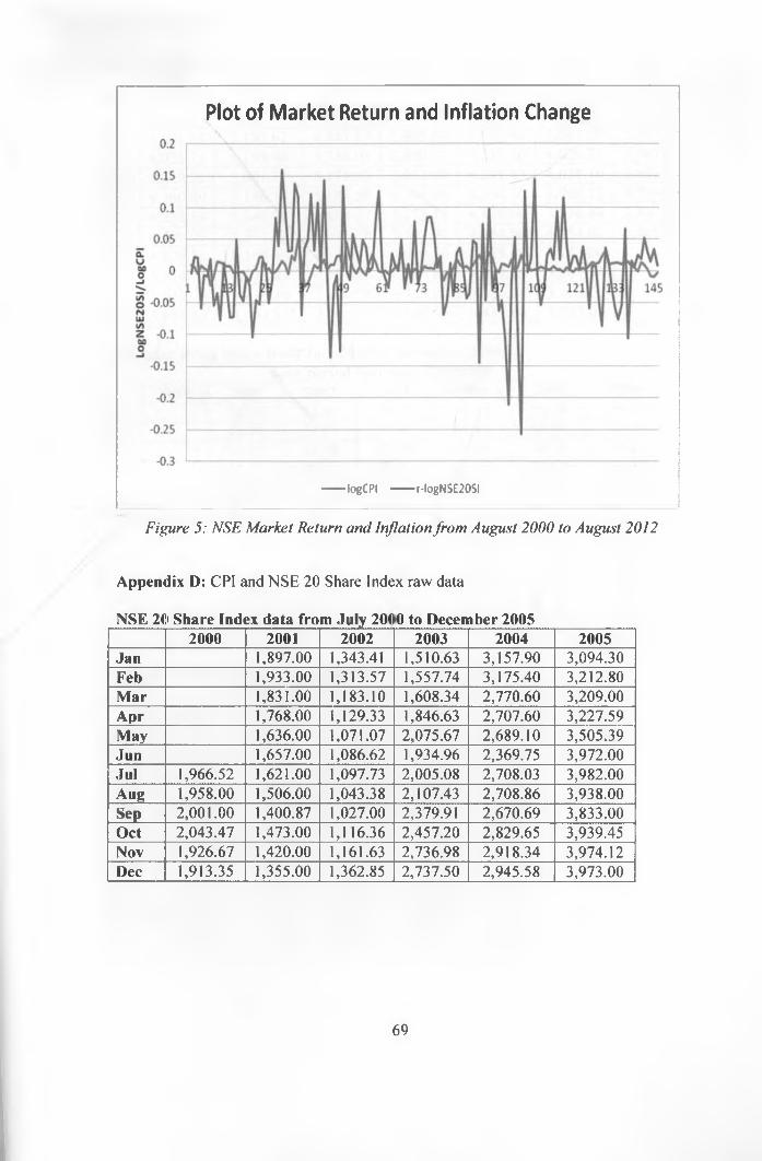
Plot of Market Return and Inflation Change

------ logCPI -------r-logNSE20SI

Figure 5: NSE Market Return and Inflation from August 2000 to August 2012

Appendix D: CPI and NSE 20 Share Index raw data

NSE 2(l Share Index data from July 20( 0 to December 20052000 2001 2002 2003 2004 2005

Jan 1,897.00 1,343.41 1,510.63 3,157.90 3,094.30Feb 1,933.00 1,313.57 1,557.74 3,175.40 3,212.80Mar 1,831.00 1,183.10 1,608.34 2,770.60 3,209.00Apr 1,768.00 1,129.33 1,846.63 2,707.60 3,227.59May 1,636.00 1,071.07 2,075.67 2,689.10 3,505.39Jun 1,657.00 1,086.62 1,934.96 2,369.75 3,972.00Jul 1,966.52 1,621.00 1,097.73 2,005.08 2,708.03 3,982.00Aug 1,958.00 1,506.00 1,043.38 2,107.43 2,708.86 3,938.00Sep 2,001.00 1,400.87 1,027.00 2,379.91 2,670.69 3,833.00Oct 2,043.47 1,473.00 1,116.36 2,457.20 2,829.65 3,939.45Nov 1,926.67 1,420.00 1,161.63 2,736.98 2,918.34 3,974.12Dec 1,913.35 1,355.00 1,362.85 2,737.50 2,945.58 3,973.00

69

NSE 20 Share Index data from January 2006 to August 20122006 2007 2008 2009 2010 2011 2012

Jan 4,171.80 5,774.24 4,712.71 3,198.90 3,565.30 4.465.00 3,224.00Feb 4,056.63 5,387.28 5,072.41 2,474.80 3.629.40 4,240.00 3,304.00Mar 4,101.64 5,133.67 4,843.17 2,805.00 4,072.90 3,887.00 3,367.00Apr 4,025.21 5,199.44 5,336.03 2,800.10 4,233.20 4,029.23 3,547.00May 4,349.75 5,001.77 5,175.83 2,852.60 4,241.80 4,078.10 3,651.00Jun 4,260.49 5,146.73 5,185.56 3,294.60 4,339.30 3,968.12 3,704.00Jul 4,258.54 5,340.08 4.868.27 3,273.10 4,438.60 3,738.46 3,832.00Aug 4,486.07 5,371.72 4,648.78 3,102.70 4,454.60 3,464.02 3,866.00Sep 4,879.86 5,146.46 4,180.40 3,005.50 4,629.80 3,283.06Oct 5,314.36 4,971.04 3,386.65 3,083.60 4,659.60 3,507.34Nov 5,615.20 5,215.36 3,341.00 3,189.60 4,395.20 3,155.00Dec 5,645.65 5,444.83 3,521.18 3,247.40 4,432.60 3,205.00

Consumer Price Index from July 2000 to December 2006Base period February 2009=100

2000 2001 2002 2003 2004 2005 2006Jan 52.60 52.85 56.21 61.35 70.48 76.22Feb 51.42 52.03 55.91 61.41 69.97 76.19Mar 50.95 51.98 57.24 62.00 70.78 76.62Apr 51.70 52.14 58.21 62.61 72.64 76.23Maj^ 52.39 53.28 61.23 64.08 73.54 76.48Jun 52.96 54.47 61.96 65.64 73.46 76.44Jul 51.20 53.38 54.51 60.46 65.62 73.34 76.30Aug 51.68 53.77 54.74 59.27 68.63 73.35 76.87Sep 52.00 53.60 54.55 58.85 70.02 73.00 77.23Oct 51.82 53.48 54.50 59.44 70.32 72.93 77.54Nov 52.28 53.40 54.77 59.69 70.07 73.33 77.82Dec 52.52 53.37 55.63 60.28 70.57 74.04 79.46

Consumer Price Index from January 2007 to August 2012Base period February 2009=1 00

2007 2008 2009 2010 2011 2012Jan 79.75 86.07 97.55 104.89 110.57 130.82Feb 78.57 87.25 100.00 105.18 112.05 130.76Mar 78.40 88.22 100.96 104.97 114.62 132.51Apr 77.76 90.85 101.84 105.56 118.29 133.74May 78.08 92.68 101.84 105.79 119.48 134.09Jun 79.53 92.89 102.05 105.61 120.91 133.06Jul 80.41 92.75 102.33 105.98 122.44 131.92A»*g 80.86 93.79 102.94 106.25 123.97 131.51Sep 81.43 94.72 103.42 106.74 125.23Oct 81.66 95.29 103.68 106.97 127.20Nov 82.47 96.95 103.87 107.86 129.13Dec 83.91 96.89 104.66 109.38 130.09

70

the impact of inflation on stock market returns and

Documents