1

DIAGNOSTIC EXPECTATIONS AND STOCK RETURNS

Pedro Bordalo, Nicola Gennaioli, Rafael La Porta, and Andrei Shleifer1

First Draft, November 2016, This Draft, September 2017

Abstract

We revisit La Porta’s (1996) finding that returns on stocks with the most optimistic analyst long term earnings growth forecasts are substantially lower than those for stocks with the most pessimistic forecasts. We document that this finding still holds, and present several further facts about the joint dynamics of fundamentals, expectations, and returns for these portfolios. We explain these facts using a new model of belief formation based on a portable formalization of the representativeness heuristic. In this model, analysts forecast future fundamentals from the history of earnings growth, but they over-react to news by exaggerating the probability of states that have become objectively more likely. Intuitively, fast earnings growth predicts future Googles but not as many as analysts believe. We test predictions that distinguish this mechanism from both Bayesian learning and adaptive expectations, and find supportive evidence. A calibration of the model offers a satisfactory account of the key patterns in fundamentals, expectations, and returns.

1 Saïd Business School, University of Oxford, Universita Bocconi and IGIER, Brown University, and Harvard University, respectively. Gennaioli thanks the European Research Council and Shleifer thanks the Pershing Square Venture Fund for Research on the Foundations of Human Behavior for financial support of this research. We are grateful to seminar participants at Brown University and Sloan School, and especially to Josh Schwartzstein, Jesse Shapiro, Pietro Veronesi, and Yang You for helpful comments. We also thank V. V. Chari, who encouraged us to confront our model of diagnostic expectations with the Kalman filter.

2

I. Introduction

La Porta (1996) shows that expectations of stock market analysts about long-term earnings

growth of the companies they cover have strong predictive power for these companies’ future

stock returns. Companies whose earnings growth analysts are most optimistic about earn poor

returns relative to companies whose earnings growth analysts are most pessimistic about.

Figure 1 offers an update of this phenomenon. Stocks are sorted by analyst long-term

earnings per share growth forecasts (LTG). The LLTG portfolio is the 10% of stocks with most

pessimistic forecasts, the HLTG portfolio is the 10% of stocks with most optimistic forecasts. The

figure reports geometric averages of one-year returns on equally weighted portfolios.

Figure 1. Annual Returns for Portfolios Formed on LTG. In December of each year between 1981 and 2015, we form decile portfolios based on ranked analysts' expected growth in earnings per share and report the geometric average one-year return over the subsequent calendar year for equally-weighted portfolios with monthly rebalancing.

Consistent with La Porta (1996), the LLTG portfolio earns an average return of 15% in the

year after formation, while the HLTG portfolio earns only 3%.2 Adjusting for systematic risk

2 The spread in Figure 1 is in line with, although smaller than, previous findings. LaPorta (1996) finds an average yearly spread of 20% but employed a shorter sample (1982 to 1991). Dechow and Sloan (1997) use a similar sample to La Porta (1996) and find a 15% spread. Appendix A shows that the spread also holds in sample subperiods.

3

deepens the puzzle: the HLTG portfolio has higher market beta than the LLTG portfolio, and

performs much worse in market downturns.3 Over the past 35 years, betting against extreme

analyst optimism has been on average a good idea. La Porta (1996) interprets this finding as

evidence that analysts, as well as investors who follow them or think like them, are too optimistic

about stocks with rapidly growing earnings, and too pessimistic about stocks with deteriorating

earnings.

In this paper we analyze the dynamics of expectation formation and offer a

psychologically founded theory that jointly accounts for the behavior of fundamentals,

expectations, and returns. We propose a new learning model in which beliefs are forward looking

just as with rational expectations, but distorted by representativeness, which biases the

interpretation of the news. Specifically, analysts update excessively in the direction of states of the

world whose objective likelihood rises the most in light of the news. The model delivers over-

reaction to news and extrapolation. It also makes sharp predictions that distinguish it from both

Bayesian learning and mechanical adaptive expectations. We test, and confirm, several of these

new predictions.

After describing the data in Section II, in Section III we document three facts. First,

HLTG stocks exhibit fast past earnings growth, which slows down going forward. Second,

forecasts of future earnings growth of HLTG stocks are excessively optimistic, and are

systematically revised downward later. Third, HLTG stocks exhibit good past returns but their

average returns going forward are low. The opposite dynamics obtain for LLTG stocks, but in a

much less extreme form, an asymmetry we do not account for in our model.

3 We find 𝛽𝛽𝐻𝐻𝐻𝐻𝐻𝐻𝐻𝐻 = 1.51, and 𝛽𝛽𝐻𝐻𝐻𝐻𝐻𝐻𝐻𝐻 = 0.78 (Appendix A). The HLTG-LLTG spread holds within size buckets and it is strongest for intermediate B/M levels.

4

Our model of learning in Section IV is based on Gennaioli and Shleifer’s (GS, 2010)

formalization of Kahneman and Tversky’s (1972) representativeness heuristic. As in GS (2010)

and Bordalo, Coffman, Gennaioli and Shleifer (BCGS, 2016), a trait 𝑡𝑡 is representative of a group

𝐺𝐺 when it occurs more frequently in that group than in a reference group −𝐺𝐺. The representative

trait 𝑡𝑡 is quickly recalled and its frequency in group 𝐺𝐺 is exaggerated. To illustrate, consider a

doctor assessing the health status of a patient after a positive test. The representative patient is

𝑡𝑡 = “sick”, because sick people are more frequent among patients who tested positive than in the

overall population. The sick patient type quickly comes to mind and the doctor inflates its

probability, which in reality may be low if the disease is rare.

In the present setting, analysts learn about firms’ unobserved fundamentals on the basis of

a noisy signal (e.g., current earnings). The rational benchmark is the Kalman Filter. Relative to

this benchmark, representativeness causes analysts to inflate the probability of firm types whose

likelihood has increased the most in light of recent earning news. After exceptionally high

earnings growth, the representative firm is a “Google”, and analysts inflate its probability. There

is a kernel of truth: Googles are truly more likely among firms exhibiting exceptional growth.

Beliefs, however, go too far: Googles are quite rare in absolute terms. Following our work on

credit cycles (BGS 2017), we say that this distorted inference follows a “Diagnostic Kalman

Filter” to emphasize that it overweighs information diagnostic of certain firm types.

Section V maps the model to the data. It starts by considering a key implication of the

kernel of truth hypothesis: expectations exaggerate the incidence of Googles in the HLTG group

because these firms are relatively more likely there. The data confirms that the HLTG group has a

fatter right tail of strong future performers than all other firms. These exceptional performers are

thus representative of the HLTG group, even though they are unlikely in absolute terms. As the

5

model predicts, we also show that analysts vastly exaggerate the share of firms with exceptional

earnings growth in the HLTG group. We then show that the model qualitatively accounts for the

joint dynamics of fundamentals, expectations, and returns documented in Section III. Intuitively,

because strong eps growth is diagnostic of future strong growth, analysts become excessively

optimistic about HLTG firms, driving up prices and generating negative forecast errors. Returns

are low post formation as analysts correct their inflated forecasts.

Section VI performs three additional exercises. Section VI.A shows that the inflated

expectations about HLTG stocks are due to over-reaction to good news. In particular, we find that

upward revisions in LTG forecasts are associated with excessive optimism (Coibion and

Gorodnichenko 2015). Section VI.B calibrates model parameters using data on the autocorrelation

of earnings and the over-reaction estimates of Section VI.A. Our simple model does a good job at

quantitatively accounting for the link between forecast errors and abnormal returns documented in

Section III. Section VI.C shows that the dynamics of expectations are hard to explain using

mechanical extrapolation: expectations mean revert even without news, suggesting that analysts

are forward looking in incorporating fundamental mean reversion into their forecasts.

Our paper is related to several strands of research in finance. Empirical research on cross-

sectional stock return predictability is framed in terms of concepts such as extrapolation (e.g.,

DeBondt and Thaler 1985, 1987, Cutler, Poterba and Summers 1991, Lakonishok, Shleifer, and

Vishny 1994, Dechow and Sloan 1997), but most studies in this area do not use expectations data.

Some older studies in finance that do use expectations data include Dominguez (1986) and

Frankel and Froot (1987, 1988). A large literature on analyst expectations shows that they are on

average too optimistic (Easterwood and Nutt 1999, Michaely and Womack 1999, Dechow,

Hutton, and Sloan 2000). More recently, the use of survey expectations data not just by analysts

6

but also by investors has been making a comeback (e.g., Ben David, Graham and Harvey 2013,

Greenwood and Shleifer 2014, Gennaioli, Ma, and Shleifer 2015).

Bouchaud, Landier, Krueger and Thesmar (2016) use analyst expectations data to study

the profitability anomaly, and offer a model in which expectations under-react to news, in contrast

with our focus on over-reaction. As we show in Section VI.A, in our data there is also some short-

term under-reaction, but at the long horizons of LTG forecasts over-reaction prevails. Daniel,

Klos, and Rottke (2017) show that stocks featuring high dispersion in analyst expectations and

high illiquidity earn high returns, but do not offer a theory of expectations and their dispersion.

Our paper is also related to research on over-reaction and volatility, which begins with

Shiller (1981), DeBondt and Thaler (1985, 1987), Cutler, Poterba, and Summers (1990), and

DeLong et al. (1990a). This work assumes mechanical, backward looking rules for belief

updating, based either on adaptive expectations (e.g., DeLong et al 1990b, Barsky and DeLong

1993, Barberis and Shleifer 2003, Barberis et al. 2015, Glaeser and Nathanson 2015), adaptive

learning (Marcet and Sargent 1989, Adam, Marcet, and Nicolini 2016, Adam, Marcet, and Beutel

2017), or rules of thumb (Hong and Stein, 1999).4 Pastor and Veronesi (2003, 2005) present

rational learning models in which uncertainty about the fundamentals of some firms boosts the

volatility of their returns and their market to book ratios. Under some conditions, learning

dynamics also explain predictability in aggregate stock returns (Pastor and Veronesi 2006). This

approach does not analyze expectations data or cross sectional differences in returns. Barberis,

Shleifer, and Vishny (BSV, 1998), Daniel, Hirshleifer, and Subramanyam (DHS, 1998) and

Odean (1998) offer models grounded in psychology. The BSV model is motivated by

representativeness, and we return to it in Section VI.C. DHS (1998) and Odean (1998) build a 4 In Adam, Marcet, and Beutel (2017), agents learn about the mapping between fundamentals and price outcomes, but hold rational expectations of fundamentals. While this approach is complementary to ours, it does not address the evidence on expectations of fundamentals that is central to our paper.

7

model of investor overconfidence, the tendency of decision-makers to exaggerate the precision of

private information, which causes divergence in beliefs and excess trading. In contrast, our model

is concerned with overreaction to public information.

One advantage of our approach worth stressing is that our model is not designed for a

specific finance setting but is more portable (Rabin 2013). Our formalization of representativeness

was developed to account for biases in general probability assessments such as base rate neglect,

conjunction and disjunction fallacies in a laboratory context (Gennaioli and Shleifer 2010). We

have previously applied it to modeling social stereotypes (Bordalo, Coffman, Gennaioli and

Shleifer 2016, 2017) and credit cycles (Bordalo, Gennaioli and Shleifer 2017), where the patterns

of over-reaction to news, systematic forecast errors, expectations revisions, and predictable

returns are similar to those discussed here.

II. Data and Summary Statistics

II.A. Data

We gather data on analysts’ expectations from IBES, stock prices and returns from CRSP,

and accounting information from CRSP/COMPUSTAT. Below we describe the measures used in

the paper and, in parentheses, provide their mnemonics in the primary datasets.

From the IBES Unadjusted US Summary Statistics file we obtain mean analysts’ forecasts

for earnings per share and their expected long-run growth rate (meanest, henceforth “LTG”) for

the period December 1981, when LTG becomes available, through December 2016. IBES defines

LTG as the “expected annual increase in operating earnings over the company’s next full business

cycle”, a period ranging from three to five years. From the IBES Detail History Tape file we get

analyst-level data on earnings forecasts. We use CRSP daily data on stock splits (cfacshr) to

8

adjust IBES earnings per share figures. On December of each year between 1981 and 2015, we

form LTG decile portfolios based on stocks that report earnings in US dollars.5

The CRSP sample includes all domestic common stocks listed on a major US stock

exchange (i.e. NYSE, AMEX, and NASDAQ) except for closed-end funds and REITs. Our

sample starts in 1978 and ends in 2016. We present results for both buy-and-hold annual returns

and daily cumulative-abnormal returns for various earnings’ announcement windows. We

compute annual stock returns by compounding monthly returns. We focus on equally-weighted

returns for LTG portfolios. If a stock is delisted, CRSP tries to establish its price after delisting.

Whenever a post-delisting price exists, we use it in the computations for returns. When CRSP is

unable to determine the value of a stock after delisting, we assume that the investor was able to

trade at the last quoted price. After a stock disappears from the sample, we replace its return until

the end of the calendar year with the return of the equally-weighted market portfolio. Given that

IBES surveys analysts around the middle of the month (on Thursday of the third week of the

month), LTG is in the information set when we form portfolios. Daily cumulative abnormal

returns are defined relative to CRSP’s equally-weighted index. We also gather data on market

capitalization in December of year t as well as the pre-formation 3-year return ending on

December of year t. Finally, we rank stocks into deciles based on market capitalization using

breakpoints for NYSE stocks.

We get from the CRSP/COMPUSTAT merged file on assets (at), sales (sale), net income

(ni), book equity, common shares used to calculate earnings per share (cshpri), adjustment factor

for stock splits (adjex_f), and Wall Street Journal dates for quarterly earnings' releases (rdq). Our

CRSP/COMPUSTAT data covers the period 1978-2016. We use annual and quarterly accounting

5 We form portfolios in December of each year, because that is when IBES data on analyst expectations is released. Unlike in Fama and French (1993) we know exactly when the information required for an investable strategy is public.

9

data. We define book equity as stockholders’ equity (depending on data availability seq, ceq+pfd,

or at-lt) plus deferred taxes (depending on data availability txditc or txdb+itcb) minus preferred

equity (depending on data availability pstkr, pstkl, or pstk). We define operating margin as the

difference between sales and cost of goods sold (cogs) and return on equity as net income divided

by book equity. We compute the annual growth rate in sales per share in the most recent 3 fiscal

years. When merging IBES with CRSP/COMPUSTAT, we follow the literature and assume that

data for fiscal periods ending after June becomes available during the next calendar year.

II.B. Summary Statistics

Table 1 reports the means of some of the variables for LTG decile portfolios. The number

of stocks with CRSP data on stock returns and IBES data on LTG varies by year, ranging from

1,310 in 1981 to 3,849 in 1997. On average, each LTG portfolio contains 241 stocks. The

forecasted growth rate in earnings per share ranges from 4% for the lowest LTG decile (LLTG) to

38% for the highest decile (HLTG), an enormous difference. LLTG stocks are larger than HLTG

stocks in terms of both total assets (7,942 MM vs. 1,081 MM) and market capitalization (3,913

MM vs. 1,749 MM). However, differences in size are not extreme: the average size decile is 5.1

for LLTG and 3.6 for HLTG.

LLTG stocks have lower operating margins to asset ratios than HLTG stocks but higher

return on equity (5% vs -6%). In fact, 31% of HLTG firms have negative eps while the same is

true for only 12% of LLTG stocks. The high incidence of negative eps companies in the HLTG

portfolio underscores the importance of the definition of LTG in terms of annual earnings growth

over a full business cycle. Current negative earnings do not hinder these firms’ future prospects.

10

Table 1 – Descriptive Statistics for Portfolios Formed on LTG. We form decile portfolios based on analysts' expected growth in earnings per share (LTG) in December of each year between 1981 and 2015. The table reports time-series means of the variables described below for equally-weighted LTG portfolios. Unless otherwise noted, accounting variables pertain to the most recently available fiscal year, where we follow the standard assumption that data for fiscal periods ending after June become available during the next calendar year. Assets is book value of total assets (in millions). Market capitalization is the value of common stock on the last trading day of year t (in millions). Size decile refers to deciles of market capitalization with breakpoints computed using only NYSE stocks. Operating margin to assets is the difference between sales and cost of goods sold divided by assets. Return on equity is net income divided by book equity. Percent eps positive is the fraction of firms with positive earnings. Observations is the number of observations in a year. All variables are capped at the 1% and 99% levels.

LTG decile 1 2 3 4 5 6 7 8 9 10 Expected growth in eps (LTG) 4% 9% 10% 12% 14% 15% 17% 20% 25% 38% Assets (MM) 7,942 10,570 10,391 7,631 5,395 3,591 2,352 1,903 1,295 1,084 Market capitalization (MM) 3,913 4,829 5,434 4,552 4,218 3,406 2,685 2,596 1,818 1,749 Size decile 5.1 5.1 5.4 5.3 5.2 4.7 4.5 4.0 3.7 3.6 Operating margin to assets 19% 25% 29% 33% 37% 40% 42% 42% 41% 36% Return on equity 5% 8% 11% 10% 10% 9% 9% 6% 1% -6% Percent eps positive 88% 90% 93% 93% 93% 91% 91% 87% 81% 69% Observations 257 245 235 242 243 257 216 253 240 227

III. A New Look at the Data.

Figure 1 suggests that analysts and the stock market may be too bullish on firms they are

optimistic about, and too bearish on firms they are pessimistic about. To assess this possibility, we

document some basic facts connecting firms’ performance, expectations and returns.

Figure 2 reports average earnings per share of HLTG and LLTG portfolios in years 𝑡𝑡 − 3

to 𝑡𝑡 + 3 where 𝑡𝑡 = 0 corresponds to portfolio formation. We normalize year 𝑡𝑡 − 3 earnings per

share of both portfolios to $1. Earnings per share for HLTG stocks exhibit explosive growth

during the pre-formation period, rising from $1 in year -3 to $1.56 in year 0. Earnings of LLTG

firms decline to $0.87 during the corresponding period. But the past does not repeat itself after

portfolio formation, because of mean reversion in earnings growth. Earnings growth of HLTG

11

firms slows down, while earnings of LLTG firms recover during the post-formation period. HLTG

firms remain more profitable on average than LLTG firms 3 years after portfolio formation, but

the difference in actual growth rates is nowhere near the difference in LTG exhibited in Table 1.

Figure 2. Evolution of EPS. In December of years (t) 1981, 1984., …,2011, and 2013, we form decile portfolios based on ranked analysts' expected growth in earnings per share (LTG). We report the mean value of earnings per share for the highest (HLTG) and lowest (LLTG) LTG deciles for each year between t-3 and t+3. We exclude firms with negative earnings in t-3 and normalize to 1 the value of earnings per share in t-3.

Figure 3 shows the average LTG for the HLTG and LLTG portfolios over the same time

window. Prior to portfolio formation, expectations of long-term growth for HLTG firms rise

dramatically in response to strong earnings growth (compare with Figure 2), while expectations

for LLTG drop. After formation, expectations for HLTG firms are revised sharply downwards,

particularly during the first year, whereas LTG of LLTG firms is revised moderately up. Three

years after portfolio formation, earnings of HLTG firms are still expected to grow faster than

those of LLTG firms, but the spread in expected growth rates of earnings has narrowed

considerably. One potential concern about Figure 2 and in other Figures in this Section is the role

of attrition in the sample. Reassuringly, the level of attrition is similar across HLTG and LLTG

12

portfolios (roughly 30% three years post formation), and the key features of the Figures continue

to hold when we restrict the sample to firms that survive for five years post formation.

Figure 3. Evolution of LTG. In December of each year t between 1984 and 2013, we form decile portfolios based on ranked analysts' expected growth in earnings per share (LTG) and report the mean value of LTG on December of years t-3 to t+3 for the highest (HLTG) and lowest (LLTG) LTG deciles. We include in the sample stocks with LTG forecasts in year t-3. Values for t+1, t+2, and t+3 are based on stocks with IBES coverage for those periods.

Expectations of long-term growth follow the pattern of actual earnings per share of HLTG

and LLTG portfolios displayed in Figure 2. Analysts seem to be learning about firms’ earnings

growth from their past performance. Fast pre-formation growth leads analysts to place a firm in

the HLTG category. Post-formation growth slowdown triggers a downward revision of forecasts.

Mean reversion in forecasts may be caused by mean reversion in fundamentals, which is

evident in Figure 2, or by the correction of analysts’ expectations errors at formation. To see the

role of expectations errors, Figure 4 reports the difference between realized earnings growth and

analysts’ LTG expectations in each portfolio, from formation to year 𝑡𝑡 + 3. There is strong over-

optimism, i.e. very negative forecast errors, for HLTG firms. There is also over-optimism for

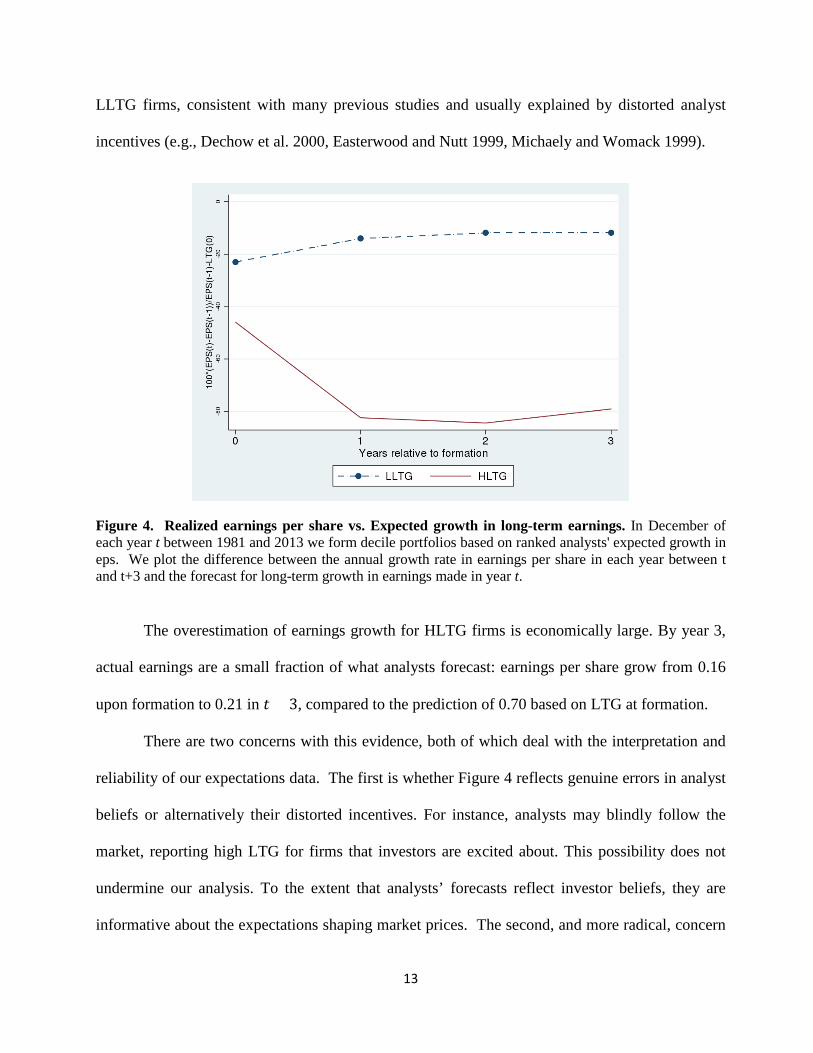
13

LLTG firms, consistent with many previous studies and usually explained by distorted analyst

incentives (e.g., Dechow et al. 2000, Easterwood and Nutt 1999, Michaely and Womack 1999).

Figure 4. Realized earnings per share vs. Expected growth in long-term earnings. In December of each year t between 1981 and 2013 we form decile portfolios based on ranked analysts' expected growth in eps. We plot the difference between the annual growth rate in earnings per share in each year between t and t+3 and the forecast for long-term growth in earnings made in year t.

The overestimation of earnings growth for HLTG firms is economically large. By year 3,

actual earnings are a small fraction of what analysts forecast: earnings per share grow from 0.16

upon formation to 0.21 in 𝑡𝑡 + 3, compared to the prediction of 0.70 based on LTG at formation.

There are two concerns with this evidence, both of which deal with the interpretation and

reliability of our expectations data. The first is whether Figure 4 reflects genuine errors in analyst

beliefs or alternatively their distorted incentives. For instance, analysts may blindly follow the

market, reporting high LTG for firms that investors are excited about. This possibility does not

undermine our analysis. To the extent that analysts’ forecasts reflect investor beliefs, they are

informative about the expectations shaping market prices. The second, and more radical, concern

14

is whether investors share analysts’ beliefs or alternatively the latter are noise. To address this

concern we look at the dynamics of stock returns pre and post formation. Figure 5 shows stock

returns around earnings announcements. For every stock in the HLTG and LLTG portfolios, we

compute the 12-day cumulative return during the four quarterly earnings announcement days, in

years 𝑡𝑡 − 3 to 𝑡𝑡 + 4, following the methodology of La Porta et al. (1997).

Figure 5. Twelve-day Returns on Earnings Announcements for LTG Portfolios. In December of each year 𝑡𝑡 between 1981 and 2013, we form decile portfolios based on ranked analysts' expected growth in earnings per share. Next, for each stock, we compute the 3-day market-adjusted return centered on earnings announcements in years 𝑡𝑡 − 3, … , 𝑡𝑡 + 3. Next, we compute the annual return that accrues over earnings announcements by compounding all 3-day stock returns in each year. We report the equally-weighted average annual return during earnings announcements for the highest (HLTG) and lowest (LLTG) LTG deciles. Excess returns are defined relative to the equally-weighted CRSP market portfolio.

HLTG stocks positively surprise investors with their earnings announcements in the years

prior to portfolio formation, when there is upward revision of LTG.6 Returns are low afterwards,

especially in year 1, consistent with the sharp decline in LTG in this period. Analysts’ over-

optimism thus seems to be shared by investors, so that HLTG stocks consistently disappoint in the 6 The persistence of positive surprises and high returns exhibited by the HLTG portfolio in Figure 5 should not be confused with time-series momentum. Instead, it arises from selection: on average, firms require a sequence of positive shocks to be classified as HLTG. The basic HLTG-LLTG spread is orthogonal to short-term return momentum in the 6 months prior to portfolio formation, see Appendix A.

15

post formation period. The converse holds for LLTG stocks, but in a milder form. In sum,

analysts’ expectations are not noise: they correlate both with actual earnings and stock returns.

Overall, three aspects of the analyst expectations evidence play a key role in our theory.

First, analysts react to news. Optimism about HLTG firms follows the observation of fast earnings

growth, and is reversed after earnings’ growth slows down. It seems that analysts are trying to

learn the earnings generating capacity of firms on the basis of past performance. Second, one

should be skeptical of analyst rationality, as shown by the evidence on systematic forecast errors

in the HLTG group (which comprises more than 200 firms). Third, the dynamics of returns match

the dynamics of expectations and their errors, both pre and post formation.

In the next section, we develop a model based on psychological first principles that sheds

light on this evidence. This model takes the perspective that the consensus analyst forecasts are

the relevant expectations that shape prices and whose dynamics drive returns. A key goal of our

approach is to simultaneously explain analysts’ forecast errors and return predictability.

Predictable returns as such could arise with full rationality: if investors have different required

returns for different firms and if analysts jointly learn a firm’s required return and its earnings.7

However, the evidence on predictable errors in expectations of both earnings and returns is

inconsistent with this possibility. We return to this point in Section VI.

IV. A model of learning with representativeness

IV.A. The Setup

7 We thank our discussant Pietro Veronesi for making this point.

16

There is a measure 1 of firms, 𝑖𝑖 ∈ [0,1]. At time 𝑡𝑡, the natural logarithm of a firm’s

earnings per share (eps) 𝑥𝑥𝑖𝑖,𝑡𝑡 is given by:

𝑥𝑥𝑖𝑖,𝑡𝑡 = 𝑏𝑏𝑥𝑥𝑖𝑖,𝑡𝑡−1 + 𝑓𝑓𝑖𝑖,𝑡𝑡 + 𝜖𝜖𝑖𝑖,𝑡𝑡, (1)

where 𝑏𝑏 ∈ [0,1] captures mean-reversion in eps, and 𝜀𝜀𝑖𝑖,𝑡𝑡 denotes a transitory i.i.d. normally

distributed shock to eps, 𝜀𝜀𝑖𝑖,𝑡𝑡~𝒩𝒩(0,𝜎𝜎𝜀𝜀2). The term 𝑓𝑓𝑖𝑖,𝑡𝑡, which we call the firm’s “fundamental”,

captures the firm’s persistent earnings capacity. It obeys the law of motion:

𝑓𝑓𝑖𝑖,𝑡𝑡 = 𝑎𝑎 ∙ 𝑓𝑓𝑖𝑖,𝑡𝑡−1 + 𝜂𝜂𝑖𝑖,𝑡𝑡. (2)

where 𝑎𝑎 ∈ [0,1] is persistence and 𝜂𝜂𝑖𝑖,𝑡𝑡~𝒩𝒩(0,𝜎𝜎𝜂𝜂2) is an i.i.d. normally distributed shock that may

for instance result from a corporate reorganization or a change in market competition. We can

think of firms with exceptionally high 𝑓𝑓𝑖𝑖,𝑡𝑡 as “Googles” that will produce very high earnings in the

future, and firms with low 𝑓𝑓𝑖𝑖,𝑡𝑡 as “lemons” that will produce low earnings in the future. We

assume stationarity of earnings by imposing the additional condition 𝑏𝑏 ≤ 𝑎𝑎.

The analyst observes eps 𝑥𝑥𝑖𝑖,𝑡𝑡 but not the fundamental 𝑓𝑓𝑖𝑖,𝑡𝑡. The Kalman filter characterizes

the forecasted distribution of 𝑓𝑓𝑖𝑖,𝑡𝑡 at any time 𝑡𝑡 conditional on the firm’s past and current earnings

�𝑥𝑥𝑖𝑖,𝑢𝑢�𝑢𝑢≤𝑡𝑡. Given the mean forecasted fundamental 𝑓𝑓𝑖𝑖,𝑡𝑡−1 for firm i at 𝑡𝑡 − 1 and its current earnings

𝑥𝑥𝑖𝑖,𝑡𝑡, the firm’s current forecasted fundamental is normally distributed with variance 𝜎𝜎𝑓𝑓2 and

mean:8

𝑓𝑓𝑖𝑖,𝑡𝑡 = 𝑎𝑎𝑓𝑓𝑖𝑖,𝑡𝑡−1 + 𝐾𝐾�𝑥𝑥𝑖𝑖,𝑡𝑡 − 𝑏𝑏𝑥𝑥𝑖𝑖,𝑡𝑡−1 − 𝑎𝑎𝑓𝑓𝑖𝑖,𝑡𝑡−1�, (3)

8 Equation (3) arises in the long run, when the variance of fundamentals has converged to its steady state 𝜎𝜎𝑓𝑓2. Given the presence of fundamental shocks 𝜂𝜂𝑖𝑖,𝑡𝑡, a firm’s fundamental is never learned with certainty. In the long run, variance stays constant at 𝜎𝜎𝑓𝑓2, which is defined as the solution to:

𝑎𝑎2𝜎𝜎𝑓𝑓4 + 𝜎𝜎𝑓𝑓2�𝜎𝜎𝜂𝜂2 + (1 − 𝑎𝑎2)𝜎𝜎𝜀𝜀2� − 𝜎𝜎𝜂𝜂2𝜎𝜎𝜀𝜀2 = 0

17

where 𝐾𝐾 ≡𝑎𝑎2𝜎𝜎𝑓𝑓

2+𝜎𝜎𝜂𝜂2

𝑎𝑎2𝜎𝜎𝑓𝑓2+𝜎𝜎𝜂𝜂2+𝜎𝜎𝜀𝜀2

is the signal to noise ratio.

The new forecast of fundamentals starts from the history-based value 𝑎𝑎𝑓𝑓𝑖𝑖,𝑡𝑡−1 but adjusts it

in the direction of the current surprise 𝑥𝑥𝑖𝑖,𝑡𝑡 − 𝑏𝑏𝑥𝑥𝑖𝑖,𝑡𝑡−1 − 𝑎𝑎𝑓𝑓𝑖𝑖,𝑡𝑡−1. The extent of adjustment increases

in 𝐾𝐾. Absent transitory shocks (𝜎𝜎𝜀𝜀2 = 0), earnings are perfectly informative about fundamentals

and the adjustment is full (i.e., 𝑓𝑓𝑖𝑖,𝑡𝑡 = 𝑥𝑥𝑖𝑖,𝑡𝑡 − 𝑏𝑏𝑥𝑥𝑖𝑖,𝑡𝑡−1). As the importance of transitory shocks rises,

earnings become a noisier signal and estimated fundamentals change less with earnings, so 𝐾𝐾 < 1.

The signal to noise ratio solves the key inference problem here: to separate the extent to

which current earnings 𝑥𝑥𝑖𝑖,𝑡𝑡 are due to persistent or transitory shocks (i.e., 𝜂𝜂𝑖𝑖,𝑡𝑡 versus 𝜀𝜀𝑖𝑖,𝑡𝑡). Among

episodes of exceptionally high growth, the analyst must try to tell apart those due to luck and

those due to the fact that the firm is the next Google.

Equation (3) yields not only the true conditional distribution of fundamentals, but also the

assessment of fundamentals performed by a Bayesian agent seeking to forecast future earnings.

We next describe how the representativeness heuristic distorts this learning process.

IV.B. Representativeness and the Diagnostic Kalman filter

Kahneman and Tversky (KT 1972) argue that the automatic use of the representativeness

heuristic causes individuals to estimate a type as likely in a group when it is merely representative

of that group. KT define representativeness as follows: “an attribute is representative of a class if

it is very diagnostic; that is, the relative frequency of this attribute is much higher in that class

than in a relevant reference class (TK 1983).” Starting with KT (1972), experimental evidence

has found ample support for the role of representativeness.

18

Gennaioli and Shleifer (2010) propose a model of this phenomenon in which a decision

maker assesses the distribution ℎ(𝑇𝑇 = 𝜏𝜏|𝐺𝐺) of a variable 𝑇𝑇 in a group 𝐺𝐺. The representativeness

of the specific type 𝜏𝜏 for 𝐺𝐺 is:

𝑅𝑅(𝜏𝜏,𝐺𝐺) ≡ℎ(𝛵𝛵 = 𝜏𝜏|𝐺𝐺)ℎ(𝑇𝑇 = 𝜏𝜏|−𝐺𝐺). (4)

As in KT, a type is more representative if it is relatively more frequent in 𝐺𝐺 than in the

comparison group –𝐺𝐺. The probability of representative types is overestimated relative to the

truth. BCGS (2016) offer a convenient formalization of this process by assuming that probability

judgments are formed using the distorted density:

ℎ𝜃𝜃(𝑇𝑇 = 𝜏𝜏|𝐺𝐺) = ℎ(𝑇𝑇 = 𝜏𝜏|𝐺𝐺) �ℎ(𝑇𝑇 = 𝜏𝜏|𝐺𝐺)ℎ(𝑇𝑇 = 𝜏𝜏| − 𝐺𝐺)

�𝜃𝜃

𝑍𝑍, (5)

where 𝜃𝜃 ≥ 0 and 𝑍𝑍 is a constant ensuring that the distorted density ℎ𝜃𝜃(𝑇𝑇 = 𝜏𝜏|𝐺𝐺) integrates to 1.

The extent of probability distortions increases in 𝜃𝜃, with 𝜃𝜃 = 0 capturing the rational benchmark.

In Kahneman and Tversky’s quote, as well as in Equation (4), the representativeness of a

type depends on its true relative frequency in the group 𝐺𝐺. The distorted probability in (5) thus

depends on the true probability, which renders the model empirically testable. GS (2010)

interpret this feature on the basis of limited and selective memory. True information ℎ(𝑇𝑇 = 𝜏𝜏|𝐺𝐺)

and ℎ(𝑇𝑇 = 𝜏𝜏| − 𝐺𝐺) about a group is stored in a decision maker’s long term memory.

Representative types, being distinctive of the group under consideration, are more readily recalled

than other types. As a result, representative types play an outsized role in judgments; other types

are relatively neglected.

This setup can be applied to prediction and inference problems (as in BCGS 2016 and

BGS 2016). Consider the example from the introduction of a doctor assessing the health status of

19

a patient, 𝑇𝑇 = {ℎ𝑒𝑒𝑎𝑎𝑒𝑒𝑡𝑡ℎ𝑦𝑦, 𝑠𝑠𝑖𝑖𝑠𝑠𝑠𝑠} in light of a positive medical test, 𝐺𝐺 = 𝑝𝑝𝑝𝑝𝑠𝑠𝑖𝑖𝑡𝑡𝑖𝑖𝑝𝑝𝑒𝑒. The positive test

is assessed in the context of untested patients (−𝐺𝐺 = 𝑢𝑢𝑢𝑢𝑡𝑡𝑒𝑒𝑠𝑠𝑡𝑡𝑒𝑒𝑢𝑢). Applying the previous

definition, being sick is representative of patients who tested positive if and only if:

Pr(𝑇𝑇 = 𝑠𝑠𝑖𝑖𝑠𝑠𝑠𝑠|𝐺𝐺 = 𝑝𝑝𝑝𝑝𝑠𝑠𝑖𝑖𝑡𝑡𝑖𝑖𝑝𝑝𝑒𝑒)Pr(𝑇𝑇 = 𝑠𝑠𝑖𝑖𝑠𝑠𝑠𝑠|−𝐺𝐺 = 𝑢𝑢𝑢𝑢𝑡𝑡𝑒𝑒𝑠𝑠𝑡𝑡𝑒𝑒𝑢𝑢) >

Pr(𝑇𝑇 = ℎ𝑒𝑒𝑎𝑎𝑒𝑒𝑡𝑡ℎ𝑦𝑦|𝐺𝐺 = 𝑝𝑝𝑝𝑝𝑠𝑠𝑖𝑖𝑡𝑡𝑖𝑖𝑝𝑝𝑒𝑒)Pr(𝑇𝑇 = ℎ𝑒𝑒𝑎𝑎𝑒𝑒𝑡𝑡ℎ𝑦𝑦|−𝐺𝐺 = 𝑢𝑢𝑢𝑢𝑡𝑡𝑒𝑒𝑠𝑠𝑡𝑡𝑒𝑒𝑢𝑢),

namely when Pr(𝐺𝐺 = 𝑝𝑝𝑝𝑝𝑠𝑠𝑖𝑖𝑡𝑡𝑖𝑖𝑝𝑝𝑒𝑒|𝑇𝑇 = 𝑠𝑠𝑖𝑖𝑠𝑠𝑠𝑠) > Pr(𝐺𝐺 = 𝑝𝑝𝑝𝑝𝑠𝑠𝑖𝑖𝑡𝑡𝑖𝑖𝑝𝑝𝑒𝑒|𝑇𝑇 = ℎ𝑒𝑒𝑎𝑎𝑒𝑒𝑡𝑡ℎ𝑦𝑦). The condition

holds if the test is even minimally informative of health status. A positive test brings “sick” to

mind because the true probability of this type has increased the most after the positive test is

revealed. Thus, the doctor may deem the sick state likely, even if the disease is rare (Casscells et

al. 1978), committing a form of base rate neglect described in TK’s (1974).

We apply this logic to the problem of forecasting a firm’s earnings. The analyst must infer

the firm’s type 𝑓𝑓𝑖𝑖,𝑡𝑡 after observing the current earnings surprise 𝑥𝑥𝑖𝑖,𝑡𝑡 − 𝑏𝑏𝑥𝑥𝑖𝑖,𝑡𝑡−1 − 𝑎𝑎𝑓𝑓𝑖𝑖,𝑡𝑡−1. This is

akin to seeing the medical test. As we saw previously, the true conditional distribution of firm

fundamentals 𝑓𝑓𝑖𝑖,𝑡𝑡 is normal, with variance 𝜎𝜎𝑓𝑓2 and the mean given by Equation (3). This is our

target distribution ℎ(𝑇𝑇 = 𝜏𝜏|𝐺𝐺). As in the medical example, the information content of the

earnings 𝑥𝑥𝑖𝑖,𝑡𝑡 for fundamentals 𝑓𝑓𝑖𝑖,𝑡𝑡 is assessed relative to the background information set in which

no news is received, namely if the earnings surprise is zero 𝑥𝑥𝑖𝑖,𝑡𝑡 − 𝑏𝑏𝑥𝑥𝑖𝑖,𝑡𝑡−1 = 𝑎𝑎𝑓𝑓𝑖𝑖,𝑡𝑡−1. The

comparison distribution ℎ(𝑇𝑇 = 𝜏𝜏| − 𝐺𝐺) is thus also, normal with mean 𝑎𝑎𝑓𝑓𝑖𝑖,𝑡𝑡−1 and variance 𝜎𝜎𝑓𝑓2.

With normality, the representativeness of fundamental 𝑓𝑓 for firm 𝑖𝑖 at date 𝑡𝑡 is:

𝑅𝑅�𝑓𝑓, 𝑥𝑥𝑖𝑖,𝑡𝑡 − 𝑏𝑏𝑥𝑥𝑖𝑖,𝑡𝑡−1� = exp ��𝑓𝑓𝑖𝑖,𝑡𝑡 − 𝑎𝑎𝑓𝑓𝑖𝑖,𝑡𝑡−1��2𝑓𝑓 − 𝑎𝑎𝑓𝑓𝑖𝑖,𝑡𝑡−1 − 𝑓𝑓𝑖𝑖,𝑡𝑡�

2𝜎𝜎𝑓𝑓2�.

If news are good, in the sense that they rationally imply better fundamentals, 𝑓𝑓𝑖𝑖,𝑡𝑡 > 𝑎𝑎𝑓𝑓𝑖𝑖,𝑡𝑡−1,

representativeness is higher for higher types 𝑓𝑓. After bad news, implying 𝑓𝑓𝑖𝑖,𝑡𝑡 < 𝑎𝑎𝑓𝑓𝑖𝑖,𝑡𝑡−1,

20

representativeness is higher for lower types 𝑓𝑓. In the first case, high types are overweighed while

low types are underweighted in judgments. In the latter case, the reverse is true.

Appendix A shows that these distortions generate diagnostic beliefs as follows:

Proposition 1 (Diagnostic Kalman filter) In the long run, upon seeing 𝑥𝑥𝑖𝑖,𝑡𝑡 − 𝑏𝑏𝑥𝑥𝑖𝑖,𝑡𝑡−1, the analyst’s

posterior about the firm’s fundamentals are normally distributed with variance 𝜎𝜎𝑓𝑓2 and mean:

𝑓𝑓𝑖𝑖,𝑡𝑡𝜃𝜃 = 𝑎𝑎𝑓𝑓𝑖𝑖,𝑡𝑡−1 + 𝐾𝐾(1 + 𝜃𝜃)�𝑥𝑥𝑖𝑖,𝑡𝑡 − 𝑏𝑏𝑥𝑥𝑖𝑖,𝑡𝑡−1 − 𝑎𝑎𝑓𝑓𝑖𝑖,𝑡𝑡−1�. (6)

When analysts overweight representative types, their beliefs resemble the optimal Kalman

filter, but with a key difference: they exaggerate the signal to noise ratio, inflating the

fundamentals of firms receiving good news and deflating those of firms receiving bad news.

Exaggeration of the signal to noise ratio is reminiscent of overconfidence, but here over-reaction

occurs with respect to public as well as private news.9 The psychology is in fact very different

from overconfidence: in our model, as in the medical test example, overreaction is caused by

neglect of base rates. After good news, the most representative firms are Googles. This firm type

readily comes to mind and the analyst exaggerates its probability, despite the fact that Googles are

rare. After bad news, the most representative firms are lemons. The analyst exaggerates the

probability of this type, despite the fact that lemons are also quite rare. Exaggeration in the

reaction to news increases in 𝜃𝜃. At 𝜃𝜃 = 0 the model reduces to rational learning.

The key property of diagnostic expectations is “the kernel of truth”: distortions in beliefs

exaggerate true patterns in the data. The kernel of truth distinguishes our approach from

alternative theories of extrapolation such as adaptive expectations or BSV (1998). As we map the

model to the facts of Sections I and II, we first show that the kernel of truth is consistent with the

9 In fact, overconfidence predicts under-reaction to public news such as earnings releases (see Daniel et al. 1998).

21

data: Googles are overweighed in the HLTG portfolio because they occur much more often there

than elsewhere.

V. The Model and the Facts

To link our model to the data we shift attention from the level of earnings to the growth

rate of earnings, which is what analysts predict when they report LTG. Denote by ℎ the horizon

over which the growth forecast applies, which is about 4 years for LTG. Define the LTG of firm 𝑖𝑖

at time 𝑡𝑡 as the firm’s expected earnings growth over this horizon, namely 𝐿𝐿𝑇𝑇𝐺𝐺𝑖𝑖,𝑡𝑡 =

𝔼𝔼𝑖𝑖,𝑡𝑡𝜃𝜃 (𝑥𝑥𝑡𝑡+ℎ − 𝑥𝑥𝑡𝑡). By Equations (1) and (6), this boils down to:

𝐿𝐿𝑇𝑇𝐺𝐺𝑖𝑖,𝑡𝑡 = −(1− 𝑏𝑏ℎ)𝑥𝑥𝑡𝑡 + 𝑎𝑎ℎ1 − (𝑏𝑏/𝑎𝑎)ℎ

1 − (𝑏𝑏/𝑎𝑎) 𝑓𝑓𝑖𝑖,𝑡𝑡𝜃𝜃 .

Expectations of long-term growth are shaped by mean reversion in eps and fundamentals. LTG is

high when firms have experienced positive news, so 𝑓𝑓𝑖𝑖,𝑡𝑡𝜃𝜃 is high, and/or when current earnings 𝑥𝑥𝑡𝑡

are low, which also raises future growth. Both conditions line up with the evidence, which shows

HLTG firms have experienced fast growth (Figure 2), and have low eps (Table 1).

We begin by testing for the kernel of truth. To this end, we first report in Figure 6 the true

distribution of future eps growth for the HLTG portfolio (blue curve) against the distribution of

future eps growth of all the other firms (orange curve).

22

Figure 6 Kernel density estimates of growth in earnings per share for LTG Portfolios. In December of years (t) 1981, 1986, …, and 2011, we form decile portfolios based on ranked analysts' expected growth in long term earnings per share (LTG). For each stock, we compute the gross annual growth rate of earnings per share between t and t+5. We exclude stocks with negative earnings in year t and we estimate the kernel densities for stocks in the highest (HLTG) decile and for all other firms with LTG data. The graph shows the estimated density kernels of growth in earnings per share for stocks in the HLTG (blue line) and all other firms (orange line). The vertical lines indicate the means of each distribution (1.11 vs. 1.08, respectively).

Two findings stand out. First, HLTG firms have a higher average future eps growth than

all other firms, as we saw in a somewhat different format in Figure 2. Second, and critically,

HLTG firms display a fatter right tail of exceptional performers. Googles are thus representative

for HLTG in the sense of definition (4). In fact, based on the densities in Figure 6, the most

representative future growth realizations for HLTG firms are in the range of 40% to 60% annual

growth.10

In light of these data, our model predicts that analysts should over-estimate the number of

right-tail performers in the HLTG group. Figure 7 compares the distribution of future performance

10 Although HLTG firms tend to have also a slightly higher share of low performers, it is true that, as in our model, higher growth rates are more representative for HLTG firms. See Figure C.1 in Appendix C.

23

of HLTG firms (blue line) with the predicted performance for the same firms (red line).11

Consistent with diagnostic expectations, analysts vastly exaggerate the share of exceptional

performers, which are most representative of the HLTG group according to the true distribution of

future eps growth.12 As a robustness check, we reproduce in Appendix C Figures 6 and 7 using as

a measure of fundamentals revenues minus cost of goods sold (which may be less noisy that eps).

With this metric as well, the evidence supports the kernel of truth hypothesis.

Figure 7. Realized vs. Expected Growth in eps. In December of years (t) 1981, 1986,…, 2006, and 2011, we form decile portfolios based on ranked analysts' expected growth in long term earnings per share (LTG). We plot two series. First, we plot the kernel distribution of the gross annual growth rate in earnings per share between t and t+5. Second, we plot the kernel distribution of the expected growth in long term earnings at time t. The graph shows results for stocks in the highest decile of expected growth in long term earnings at time t. The vertical lines indicate the means of each distribution (1.11 vs. 1.39, respectively).

We next show that the model accounts for the previously documented facts. To explore the

dynamics of LTG in our model, we focus on the long run distribution of fundamentals 𝑓𝑓𝑖𝑖,𝑡𝑡 (which

11 In making this comparison, bear in mind that analysts report point estimates of a firm’s future earnings growth and not its full distribution (in our model, they report only the mean 𝑓𝑓𝑖𝑖,𝑡𝑡𝜃𝜃 and not the variance 𝜎𝜎𝑓𝑓2). Thus, under rationality the LTG distribution would have the same mean but lower variance than realized eps growth. 12 The kernel of truth can also shed light on the asymmetry between HLTG and LLTG firms. In Appendix C we show that future performance of LLTG firms tends to be concentrated in the middle, with a most representative growth rate of 0%. It is thus constant, rather than bad, performance that is representative of LLTG firms. This fact can help explain why expectations about these firms and their market values are not overly depressed. One could capture this difference between HLTG firms (representative high growth) and LLTG firms (representative 0% growth) by relaxing the assumption of normality, or alternatively by allowing lower volatility for firms in the LLTG group.

24

has zero mean and variance 𝜎𝜎𝜂𝜂2

1−𝛼𝛼2) and of analysts’ mean beliefs 𝑓𝑓𝑖𝑖,𝑡𝑡𝜃𝜃 (which has zero mean and

variance 𝜎𝜎𝑓𝑓𝜃𝜃2 ).13 In line with our empirical analysis, at time 𝑡𝑡 we identify the high LTG group

HLTGt as the 10% of firms with highest believed fundamentals, and hence with highest assessed

future earnings growth, and the low LTG group LLTGt as the 10% of firms with lowest believed

fundamentals and hence lowest assessed future earnings growth.

V.A. Representativeness and the Features of Expectations

We first review the patterns of fundamentals and expectations documented in Figures 2, 3

and 4. In Section V.B, we review the patterns of returns documented in Figures 1 and 5.

We start from Figure 2, which says that HLTG firms experience a period of pronounced

growth before portfolio formation, while LLTG firms experience a period of decline.

Proposition 2. Provided 𝑎𝑎, 𝑏𝑏,𝐾𝐾, 𝜃𝜃 satisfy

𝑏𝑏ℎ + 𝑎𝑎ℎ1 − (𝑏𝑏/𝑎𝑎)ℎ

1 − (𝑏𝑏/𝑎𝑎) �𝐾𝐾(1 + 𝜃𝜃) − 𝑎𝑎

1 − 𝑎𝑎� > 1, (7)

the average 𝐻𝐻𝐿𝐿𝑇𝑇𝐺𝐺𝑡𝑡 (𝐿𝐿𝐿𝐿𝑇𝑇𝐺𝐺𝑡𝑡) firm experiences positive (negative) earnings growth pre-formation.

In our model, positive earnings surprises have two conflicting effects on long term growth

prospects and thus on LTG. On the one hand, they raise estimated fundamentals 𝑓𝑓𝑖𝑖,𝑡𝑡𝜃𝜃 , which

enhance future growth. On the other hand, they lower future growth via mean reversion.

Condition (7) ensures that the former effect dominates, so that firms with rosy future prospects

13 There is no distortion in the average diagnostic expectation across firms because in steady state there are no systematic earnings surprises: the average earnings news in the population of firms is zero. As a consequence, the average diagnostic expectation coincides with the average rational expectation. However, diagnostic beliefs are fatter-tailed than rational ones, because they exaggerate the frequency of Googles and Lemons.

25

(HLTG) are selected from those that have experienced good recent performance, while firms with

bad prospects (LLTG) are selected from those that have experienced bad recent performance.

The parametric restriction of Condition (7) is more likely to hold the less severe is mean

reversion (i.e., when 𝑏𝑏 is close to 1) and the larger is the signal to noise ratio 𝐾𝐾. It is also more

likely to hold the larger is 𝜃𝜃 and for relatively large 𝑎𝑎 (with 𝑎𝑎 < 𝐾𝐾(1 + 𝜃𝜃)). Note that condition

(7) depends on the parameters of the true earnings process because analysts do not mechanically

extrapolate past performance.

Combined with mean reversion of earnings, Proposition 2 accounts for Figure 2, in which

HLTG firms experience positive growth pre-formation, which subsequently cools off, while

LLTG firms go through the opposite pattern.

We next show that the model can account for the fact documented in Figure 4, namely that

expectations for the long term growth of HLTG firms are excessively optimistic.

Proposition 3. If analysts are rational, 𝜃𝜃 = 0, they make no systematic error in predicting the log

growth of earnings of HLTG𝑡𝑡 and LLTG𝑡𝑡 portfolios:

𝔼𝔼�𝑥𝑥𝑡𝑡+ℎ − 𝑥𝑥𝑡𝑡 − 𝐿𝐿𝑇𝑇𝐺𝐺𝑡𝑡𝜃𝜃=0|HLTG𝑡𝑡 � = 𝔼𝔼�𝑥𝑥𝑡𝑡+ℎ − 𝑥𝑥𝑡𝑡 − 𝐿𝐿𝑇𝑇𝐺𝐺𝑡𝑡𝜃𝜃=0|LLTG𝑡𝑡 � = 0.

Under diagnostic expectations 𝜃𝜃 > 0, in contrast, analysts systematically over-estimate growth in

HLTG𝑡𝑡 and under-estimate growth in LLTG𝑡𝑡:

𝔼𝔼�𝑥𝑥𝑡𝑡+ℎ − 𝑥𝑥𝑡𝑡 − 𝐿𝐿𝑇𝑇𝐺𝐺𝑡𝑡𝜃𝜃>0|HLTG𝑡𝑡 � < 0 < 𝔼𝔼�𝑥𝑥𝑡𝑡+ℎ − 𝑥𝑥𝑡𝑡 − 𝐿𝐿𝑇𝑇𝐺𝐺𝑡𝑡𝜃𝜃>0|LLTG𝑡𝑡 �.

Under rational expectations, no systematic forecast error can be detected by an

econometrician looking at the data (expectations are computed using the true steady state

26

probability measure). Indeed, when 𝜃𝜃 = 0, the average forecast within the many firms of the

HLTG𝑡𝑡 and LLTG𝑡𝑡 portfolios is well calibrated to the respective means. Diagnostic expectations,

in contrast, cause systematic errors. Firms in the HLTG𝑡𝑡 group are systematically over-valued:

analysts over-react to their pre-formation positive surprises, and form excessively optimistic

forecasts of fundamentals. As a consequence, the realized earnings growth is on average below

the forecast. Firms in the LLTG𝑡𝑡 group are systematically under-valued. As a consequence, their

realized earnings growth is on average above the forecast. As noted in Section III, the prediction

of systematic pessimism about LLTG firms is not borne out in the data.

Finally, our model also yields the boom-bust LTG pattern in the HLTG group (and a

reverse pattern in the LLTG group) documented in Figure 3. By Proposition 2, the improving pre-

formation forecasts of HLTG firms are due to positive earnings surprises, while the deteriorating

pre formation forecasts of LLTG firms are due to negative ones. But the model also predicts post

formation reversals in LTG for both groups of firms. To see this, we compare 𝐿𝐿𝑇𝑇𝐺𝐺𝑖𝑖,𝑡𝑡 forecasts

made at 𝑡𝑡, with forecasts made for the same firm at 𝑡𝑡 + 𝑠𝑠, namely 𝐿𝐿𝑇𝑇𝐺𝐺𝑖𝑖,𝑡𝑡+𝑠𝑠.

Proposition 4 Under rational expectations, 𝜃𝜃 = 0, we have that:

𝔼𝔼�LTG𝑡𝑡+𝑠𝑠𝜃𝜃=0|𝐻𝐻𝐿𝐿𝑇𝑇𝐺𝐺𝑡𝑡� − 𝔼𝔼�LTG𝑡𝑡

𝜃𝜃=0|𝐻𝐻𝐿𝐿𝑇𝑇𝐺𝐺𝑡𝑡� < 0

Under diagnostic expectations, 𝜃𝜃 > 0, we have that:

𝔼𝔼�LTG𝑡𝑡+𝑠𝑠𝜃𝜃>0|𝐻𝐻𝐿𝐿𝑇𝑇𝐺𝐺𝑡𝑡� − 𝔼𝔼�LTG𝑡𝑡

𝜃𝜃>0|𝐻𝐻𝐿𝐿𝑇𝑇𝐺𝐺𝑡𝑡� = 𝔼𝔼�LTG𝑡𝑡+𝑠𝑠𝜃𝜃=0|𝐻𝐻𝐿𝐿𝑇𝑇𝐺𝐺𝑡𝑡� − 𝔼𝔼�LTG𝑡𝑡

𝜃𝜃=0|𝐻𝐻𝐿𝐿𝑇𝑇𝐺𝐺𝑡𝑡� − 𝜃𝜃𝜃𝜃

for some 𝜃𝜃 > 0. The opposite pattern, with reversed inequality and 𝜃𝜃 < 0, occurs for 𝐿𝐿𝐿𝐿𝑇𝑇𝐺𝐺𝑡𝑡.

Mean reversion in LTG obtains under rational expectations, due to mean reversion in

fundamentals. Under diagnostic expectations, however, mean reversion is amplified by the

27

correction of initial forecast errors. Post-formation, the excess optimism of HLTG firms on

average dissipates, causing a cooling off in expectations 𝜃𝜃𝜃𝜃 that is more abrupt than what would

be implied by mean reversion alone. The cooling off of excess optimism arises because there are

no news on average in the HLTG portfolio, which on average causes no overreaction. Likewise,

the excess pessimism of LLTG firms dissipates, strengthening the reversal in that portfolio.14

V.B. The diagnostic Kalman filter and returns

Consider now the return patterns documented in Figures 1 and 5. To explore the

implications of diagnostic expectations for portfolio returns, we take the required return 𝑅𝑅 > 1 as

given. The pricing condition for a firm 𝑖𝑖 at date 𝑡𝑡 is then given by:

𝔼𝔼𝑡𝑡𝜃𝜃 �𝑃𝑃𝑖𝑖,𝑡𝑡+1 + 𝐷𝐷𝑖𝑖,𝑡𝑡+1

𝑃𝑃𝑖𝑖,𝑡𝑡� = 𝑅𝑅, (8)

so that the stock price of firm 𝑖𝑖 is the discounted stream of expected future dividends as of 𝑡𝑡. We

assume that 𝑅𝑅 is high enough that the discounted sum converges. By Equation (8), the equilibrium

price at 𝑡𝑡 is 𝑃𝑃𝑖𝑖,𝑡𝑡 = 𝔼𝔼𝑡𝑡𝜃𝜃�𝑃𝑃𝑖𝑖,𝑡𝑡+1 + 𝐷𝐷𝑖𝑖,𝑡𝑡+1�/𝑅𝑅. Using this formula and Proposition 2, we find:

Proposition 5. Denote by 𝑅𝑅𝑡𝑡,𝑃𝑃 the realized return of portfolio 𝑃𝑃 = 𝐻𝐻𝐿𝐿𝑇𝑇𝐺𝐺, 𝐿𝐿𝐿𝐿𝑇𝑇𝐺𝐺 at 𝑡𝑡. Then, under

the condition of Proposition 2, we have that:

𝑅𝑅𝑡𝑡,𝐻𝐻𝐻𝐻𝐻𝐻𝐻𝐻 > 𝑅𝑅 > 𝑅𝑅𝑡𝑡,𝐻𝐻𝐻𝐻𝐻𝐻𝐻𝐻

14 Going forward, firms in the HLTG portfolio receive neither positive nor negative true surprises on average, namely 𝔼𝔼𝑡𝑡�𝑥𝑥𝑖𝑖,𝑡𝑡+1 − 𝑏𝑏𝑥𝑥𝑖𝑖,𝑡𝑡−1 − 𝑎𝑎𝑓𝑓𝑖𝑖,𝑡𝑡� = 0. As a result, by Equation (6), their assessed fundamentals on average coincides with the rational value 𝑎𝑎𝑓𝑓𝑖𝑖,𝑡𝑡. The same logic triggers mean reversion in the LLTG portfolio.

28

Because firms in the HLTG portfolio receive positive news before formation (Proposition 2), they

earn returns higher than the required return 𝑅𝑅. Our model thus yields positive abnormal pre-

formation returns for HLTG stocks, as well as the low pre-formation returns of LLTG stocks, as

in Figure 5. This effect does not rely on representativeness, as it arises also for 𝜃𝜃 = 0. The key

implication of representativeness is predictability of post-formation returns (Figures 1 and 5).

To see this, note that the average realized return going forward (according to the true

probability measure) for a given firm 𝑖𝑖:

𝔼𝔼𝑡𝑡 �𝑃𝑃𝑖𝑖,𝑡𝑡+1 + 𝐷𝐷𝑖𝑖,𝑡𝑡+1

𝑃𝑃𝑖𝑖,𝑡𝑡� =

𝔼𝔼𝑡𝑡�𝑃𝑃𝑖𝑖,𝑡𝑡+1 + 𝐷𝐷𝑖𝑖,𝑡𝑡+1�𝔼𝔼𝑡𝑡𝜃𝜃�𝑃𝑃𝑖𝑖,𝑡𝑡+1 + 𝐷𝐷𝑖𝑖,𝑡𝑡+1�

𝑅𝑅. (9)

The average realized return at 𝑡𝑡 + 1 is below the required return 𝑅𝑅 when at 𝑡𝑡 investors over-value

the future expected price and dividend of firm 𝑖𝑖, namely when the denominator is larger than the

numerator in Equation (9). Conversely, the average realized return at 𝑡𝑡 + 1 is higher than the

required return 𝑅𝑅 when at 𝑡𝑡 investors under-value the firm’s future expected price and dividend.

Diagnostic expectations thus yield the return predictability patterns of Figure 5.

Proposition 6. (Predictable Returns) Denote by 𝔼𝔼𝑡𝑡�𝑅𝑅𝑡𝑡+1𝜃𝜃 |𝑃𝑃� the average future return of

portfolio 𝑃𝑃 = HLTG, LLTG at 𝑡𝑡 + 1. Under rationality, 𝜃𝜃 = 0, excess returns are not predictable:

𝔼𝔼𝑡𝑡�𝑅𝑅𝑡𝑡+1𝜃𝜃=0|𝐻𝐻𝐿𝐿𝑇𝑇𝐺𝐺� = 𝑅𝑅 = 𝔼𝔼𝑡𝑡�𝑅𝑅𝑡𝑡+1𝜃𝜃=0|𝐿𝐿𝐿𝐿𝑇𝑇𝐺𝐺�

Diagnostic expectations generate predictable excess returns:

𝔼𝔼𝑡𝑡�𝑅𝑅𝑡𝑡+1𝜃𝜃>0|𝐻𝐻𝐿𝐿𝑇𝑇𝐺𝐺� < 𝑅𝑅 < 𝔼𝔼𝑡𝑡�𝑅𝑅𝑡𝑡+1𝜃𝜃>0|𝐿𝐿𝐿𝐿𝑇𝑇𝐺𝐺�

29

Under rational expectations (i.e., for 𝜃𝜃 = 0) realized returns may differ from the required

return 𝑅𝑅 for particular firms. However, the rational model cannot account for systematic return

predictability in a large portfolio of firms sharing a certain forecast. Conditional on current

information, rational forecasts are on average (across firms) correct and returns are unpredictable.

Under the diagnostic Kalman filter (𝜃𝜃 > 0), in contrast, the HLTG portfolio exhibits

abnormally high returns up to portfolio formation and abnormally low returns after formation. The

converse holds for the LLTG portfolio, just as we saw in Table 1 and Figure 1. This is because

post-formation expectations systematically revert to fundamentals, and in particular investors are

systematically disappointed in HLTG firms and their returns are abnormally low.

To summarize, the return predictability documented in Figure 1 can be accounted by

representativeness but not by rational learning. Rational learning can account for the pre-

formation return patterns (Proposition 5), but it does not yield post formation reversals

(Proposition 6) whereby HLTG stocks underperform LLTG stocks.

VI. Additional Predictions of the Model

Diagnostic expectations yield a coherent account of the dynamics of news, analyst

expectations, and returns documented in Section III. Three issues remain open. The first is

whether analyst expectations (and hence returns) indeed over-react to news. The challenge of

testing this hypothesis is that news are hard to measure, as they include but are not restricted to

observed earnings. The second issue is whether our model can account quantitatively, and not

only qualitatively, for the dynamics of analyst expectations and returns of Section III. A third

30

issue is whether the diagnostic Kalman filter improves upon existing theories of non-rational

expectations such as BSV’s (1998) model of investor sentiment or adaptive expectations.

This section addresses these issues by highlighting additional implications of our model.

We assess the role of over-reaction in Section VI.A, the quantitative performance of the model in

Section VI.B, and alternative models of expectations formation in Section VI.C. In this last

section, we also revisit the possibility that analysts may be learning rationally from prices about

investors’ time varying required returns. As we noted in Section III, this theory does not account

for expectations errors, but it could account for return predictability.

VI.A Overreaction to News and Returns

To assess over-reaction to news, we first need to have a measure of news. Coibion and

Gorodnichenko (2015) propose measuring the news received by the forecaster at time 𝑡𝑡 using their

forecast revision at 𝑡𝑡. Such revision can in fact be interpreted as a summary for all information

received by the forecaster in the recent past. Forecasters’ over or under reaction to information

can then be assessed by correlating their forecast revision with the subsequent forecast error.

In particular, Coibion and Gorodnichenko show that in sticky information or rational

inattention models (Sims 2003, Mankiw and Reis 2002), consensus forecast revisions should

positively correlate with subsequent consensus forecast errors. Intuitively, when expectations

under-react, a positive forecast revision indicates insufficient upward adjustment. As a result, it

should predict positive errors (i.e. realizations above the forecast). Bouchaud et al. (2016) use this

method to diagnose under-reaction to news about firms’ profitability. The same approach turns

out to be useful for our analysis as well.

31

Proposition 7. Assume the condition (7) of Proposition 2. Consider the firm level regression

𝑥𝑥𝑖𝑖,𝑡𝑡+ℎ − 𝑥𝑥𝑖𝑖,𝑡𝑡 − 𝐿𝐿𝑇𝑇𝐺𝐺𝑖𝑖,𝑡𝑡 = 𝛼𝛼 + 𝛾𝛾�𝐿𝐿𝑇𝑇𝐺𝐺𝑖𝑖,𝑡𝑡 − 𝐿𝐿𝑇𝑇𝐺𝐺𝑖𝑖,𝑡𝑡−𝑘𝑘� + 𝑝𝑝𝑖𝑖,𝑡𝑡+ℎ. (10)

Under rationality, 𝜃𝜃 = 0, the estimated 𝛾𝛾 is zero, while it is negative for 𝜃𝜃 > 0.

If analysts overreact – namely 𝜃𝜃 > 0 – as predicted by diagnostic expectations, an upward

revision in LTG is symptomatic of excessive adjustment, which in turn predicts a negative

forecast error (LTG above realized growth), namely 𝛾𝛾 < 0. In contrast, under rational

expectations, forecast errors should be unpredictable at the individual level.15

Table 2 below reports the estimates from the univariate regression of forecast error,

defined as the difference between average growth over ℎ = 3,4,5 years and current LTG, and the

revision of LTG over the past 𝑠𝑠 = 1,2,3 years. We allow horizon ℎ to vary because LTG refers to

growth over a period between 3 to 5 years. To estimate 𝛾𝛾 we use consensus forecasts rather than

individual analyst estimates because many analysts drop out of the sample.16

Table 2: Coibion-Gorodnichenko regressions for EPS

Each entry in the table corresponds to the estimated coefficient of the forecast errors (epst+n/ epst)1/n-LTGt for n=3, 4, and 5 on the variables listed in the first column of the table and year fixed-effects (not shown).

Dependent Variable

(epst+3 / epst)1/3-LTGt (epst+4 / epst)1/4-LTGt (epst+5 / epst)1/5-LTGt LTGt-LTGt-1 -0.0351 -0.1253c -0.1974a (0.0734) (0.0642) (0.0516)

15 A positive estimate of 𝛾𝛾 would suggest, in our model, that analysts discount highly representative types. This is equivalent to having a negative 𝜃𝜃 in Equation (5). 16 Estimating (10) on the consensus LTG may misleadingly indicate under-reaction if individual analysts observe noisy signals, so that there is dispersion in their forecasts. Coibion and Gorodnichenko show that when different analysts observe noisy signals, the coefficient in Equation (10) is positive even if each analyst rationally revises his forecast. In this respect, finding negative 𝛾𝛾 in a consensus regression is even stronger evidence of over-reaction to information.

32

LTGt-LTGt-2 -0.2335a -0.2687a -0.2930a (0.0625) (0.0602) (0.0452)

LTGt-LTGt-3 -0.2897a -0.2757a -0.3127a (0.0580) (0.0565) (0.0437)

Consistent with diagnostic expectations, upward LTG revision predicts excess optimism,

pointing to over-reaction to news. This holds regardless of the forecast horizon ℎ, so the pattern is

robust to alternative interpretations of LTG. The estimated 𝛾𝛾 tends to become more negative and

more statistically significant at longer forecast horizons ℎ = 3,4,5 (i.e. as we move from left to

right in Table 2), perhaps reflecting the difficulty of projecting growth into the future.17

Interestingly, the estimated 𝛾𝛾 also gets higher in magnitude and more statistically

significant as we lengthen the revision period 𝑠𝑠 = 1,2,3 (i.e. moving from top to bottom in Table

2). We view this evidence as being consistent with the kernel of truth. From Equation (6), over-

reaction to information of the diagnostic filter 𝑓𝑓𝑖𝑖,𝑡𝑡𝜃𝜃 compared to the rational filter 𝑓𝑓𝑖𝑖,𝑡𝑡 is given by:

𝑓𝑓𝑖𝑖,𝑡𝑡𝜃𝜃 − 𝑓𝑓𝑖𝑖,𝑡𝑡 = 𝐾𝐾𝜃𝜃�𝑥𝑥𝑖𝑖,𝑡𝑡 − 𝑏𝑏𝑥𝑥𝑖𝑖,𝑡𝑡−1 − 𝑎𝑎𝑓𝑓𝑖𝑖,𝑡𝑡−1�,

where 𝐾𝐾 is the true signal to noise ratio of information accruing during the revision period. It is

plausible that persistent signals over 2 or 3 years are objectively more informative about future

earnings, i.e. have a higher 𝐾𝐾, than occasional signals accruing over one year. By the kernel of

truth, then, such signals should induce more over-reaction, consistent with the data.

17 This feature helps reconcile our evidence with the sluggishness documented by Bouchaud et al. (2016). They consider forecasts for the level of eps over short horizons such as 1 or 2 years. In Appendix D (see Table D.2) we show that at these horizons there is some evidence of under-reaction also in our data (with the usual caveat of the under-reaction bias entailed in estimating consensus regressions). The seemingly contradictory findings of over and under-reaction can be reconciled by combining diagnostic expectation with some short run rigidity in analyst forecasts, stemming for instance from sporadic revision times. In this case, a piece of news would initially trigger few adjustments, generating short term aggregate under-reaction, but will lead to overreaction as all analysts update.

33

To the extent that over-reaction drives excess optimism about HLTG, and thus lower post

formation returns, stronger over-reaction should be associated with larger return spreads between

HLTG and LLTG portfolios. In Appendix D.3 we show that industries in which overreaction is

larger (i.e. 𝛾𝛾 is larger) also feature larger return spreads. While these results should be taken with

caution due to the small number of industries, they are suggestive of a direct link between

overreaction and predicable returns.

Overall, this subsection offers evidence in support of the hypothesis that expectation

formation about LTG features over-reaction to news, consistent with diagnostic expectations, but

inconsistent with rational inattention or other theories of under-reaction.18

VI.B Model Calibration

We now provide a back of the envelope calibration of our model. Among other things,

this exercise yields an estimate of the strength 𝜃𝜃 of representativeness, quantifying the extent of

departures from rationality in expectations and returns.

The dynamics of firm level earnings and expectations depend on five parameters: the

persistence and conditional variance of observed log earnings per share (𝑏𝑏 and 𝜎𝜎𝜖𝜖 from Equation

1), those of fundamentals 𝑓𝑓 (𝑎𝑎 and 𝜎𝜎𝜂𝜂 from Equation 2), and the strength of representativeness 𝜃𝜃.

To predict returns, we also need to pin down the value of the required rate of return 𝑅𝑅.

18 The evidence of the over-reaction to news of consensus LTG forecasts is also inconsistent with theories of over-reaction based on analyst overconfidence such as Daniel et al. (1998). In these models, analysts over-react to their private information but under-react to common information, generating under-reaction of consensus forecasts.

34

We set the five parameters �𝑎𝑎, 𝑏𝑏,𝜎𝜎𝜂𝜂 ,𝜎𝜎𝜖𝜖 ,𝜃𝜃� to match the autocorrelation of earnings per

share of order 1, 2, 3, and 4, and the coefficient 𝛾𝛾 estimated in Section VI.A linking forecast error

�𝑒𝑒𝑒𝑒𝑠𝑠𝑡𝑡+4𝑒𝑒𝑒𝑒𝑠𝑠𝑡𝑡

�1/4

− 𝐿𝐿𝑇𝑇𝐺𝐺𝑡𝑡 to forecast revision 𝐿𝐿𝑇𝑇𝐺𝐺𝑡𝑡 − 𝐿𝐿𝑇𝑇𝐺𝐺𝑡𝑡−3.19

We fix a parameter combination �𝑎𝑎, 𝑏𝑏,𝜎𝜎𝜂𝜂 ,𝜎𝜎𝜖𝜖 ,𝜃𝜃�, simulate the model, and compute the

implied value for the five moments we seek to match. This yields the vector:

𝑝𝑝�𝑎𝑎, 𝑏𝑏,𝜎𝜎𝜂𝜂 ,𝜎𝜎𝜖𝜖 ,𝜃𝜃� = (𝜌𝜌�1,𝜌𝜌�2,𝜌𝜌�3,𝜌𝜌�4, 𝛾𝛾�),

where 𝜌𝜌�𝑙𝑙 = 𝑐𝑐𝑐𝑐𝑐𝑐(𝑥𝑥𝑡𝑡,𝑥𝑥𝑡𝑡−𝑙𝑙)𝑐𝑐𝑎𝑎𝑣𝑣(𝑥𝑥𝑡𝑡) is the model implied autocorrelation of (log) earnings of order 𝑒𝑒 (years),

and 𝛾𝛾� is coefficient obtained by estimating Equation (10) using the data generated by the model

under the same parameter combination.

We repeat the above exercise for each parameter combination �𝑎𝑎, 𝑏𝑏,𝜎𝜎𝜂𝜂 ,𝜎𝜎𝜖𝜖 ,𝜃𝜃� in a grid

defined by 𝑎𝑎, 𝑏𝑏 ∈ [0,1], 𝜎𝜎𝜂𝜂 ,𝜎𝜎𝜖𝜖 ∈ [0,0.5] and 𝜃𝜃 ∈ [0, 3] (in steps of 0.1). We calibrate the

parameters by picking the combination that minimizes the Euclidean distance loss function

ℓ(𝑝𝑝) = ‖𝑝𝑝 − �̅�𝑝‖

where �̅�𝑝 is the vector of target moments estimated from the pooled data of all firms, given by:

�̅�𝑝 = (0.82, 0.75, 0.70, 0.65,−0.282).

The table below reports the average and standard deviation of the ten parameter

combinations that yield the lowest value of the Euclidean loss function.

19 The parameters of the model could in principle be estimated by fitting a Kalman filter to the data of individual firms, but this is hampered by the fact that the time series of annual data is short, and can have negative earnings (which are assumed away in the model). For this reason, we calibrate the model by matching moments of the pooled data. We estimate autocorrelation coefficients by pooling all the observations in our dataset and running univariate OLS regressions of log earnings on its lagged value.

35

Table 3: Calibration of model parameters

𝑎𝑎 𝑏𝑏 𝜎𝜎𝜂𝜂 𝜎𝜎𝜖𝜖 𝜃𝜃

0.90

(0.01)

0.33

(0.07)

0.15

(0.05)

0.17

(0.05)

1.22

(0.18)

The high value of 𝑎𝑎 means that fundamentals are estimated to be persistent. The relatively

low value of 𝑏𝑏 then implies that shocks to log earnings mean revert fast. The variance of

fundamentals 𝜎𝜎𝜂𝜂 and of transitory earnings 𝜎𝜎𝜖𝜖 are estimated to be similar. As a first sanity check

for our calibrated log-earnings process, we can compare it to the estimates of the persistence of

earnings from the large accounting literature. This literature typically fits AR(1) processes for log

earnings to the data, and finds that estimates of the auto-regressive coefficient range from 0.77 to

0.84 with a mode at 0.8 (Sloan 1996). If we fit an AR(1) to the data simulated with the calibrated

parameters, we estimate a persistence coefficient of 0.82, very close to its empirical counterpart.

Our calibration yields a positive 𝜃𝜃, which entails over-reaction to news, and the value of

1.22 is fairly close to the estimate for the same parameter obtained by BGS (2017) in the context

of credit spreads (𝜃𝜃 = 0.91). A 𝜃𝜃 of the order of one intuitively implies that the magnitude of

forecast errors is comparable to the magnitude of news (i.e., in the current context, it implies a

doubling of the signal to noise ratio).

Finally, we calibrate the required rate of return on stocks to 𝑅𝑅 = 9.7%, which is the

historical value-weighted average market return. Using these six calibrated parameters, we

reproduce and report in Figure 8 the simulated versions of Figures 1 through 6.

36

Figure 8. Simulation of the calibrated model. Using the parameters in Table 3, and 𝑅𝑅 = 9.7%, we simulate 4000 firms over 100 time periods, generating time series of fundamentals, earnings, and growth expectations. At each time period 𝑡𝑡, we sort firms on LTG forecasts. Panel 1 shows the average return spread 1 year post-formation across LTG deciles. We first compute, for each period 𝑡𝑡, the arithmetic average return for each portfolio. We then compute the geometric average of portfolio returns over time. Panels 2, 3, and 5 show the average EPS, LTG, and returns of the HLTG and LLTG portfolios from year 𝑡𝑡 − 3 to year 𝑡𝑡 + 3. Panel 4 shows the forecast error on HLTG and LLTG portfolios in the 5 years porst-formation. Panel 6 shows the distribution of realized earnings growth after 5 years for HLTG and for non-HLTG firms, together with the forecast for growth after 5 years.

The model reproduces the main qualitative features of the data. In Panel 1, it reproduces

the return spread between HLTG and LLTG stocks. In Panel 2, it reproduces the pattern of Figure

2 that pre-formation HLTG firms have fast growth, which then declines post formation. In Panel

3 the model reproduces the boom bust dynamics of LTG, with analysts’ expectations becoming

more optimistic pre-formation, and then reverting post-formation. Panel 4 reproduces the finding

37

of Figure 4 of large forecast errors (excess optimism) for HLTG stocks.20 Panel 5 reproduces the

boom-bust pattern in returns around portfolio formation. Returns for HLTG stocks are very high

pre-formation, but then collapse below the required return 𝑅𝑅 in the immediate post formation

period, and eventually reverting back to their unconditional, long term value. The opposite

happens to the return of LLTG stocks. Finally, and crucially, the model exhibits the kernel of

truth, in that HLTG firms do perform better going forward than non-HLTG firms (panel 6).21

The model fails to capture some qualitative features of the data. It does not capture the

persistent high earnings growth of HLTG stocks before formation, nor the negative forecast error

for LLTG. We return to these issues when we summarize the results of the calibration.

We now assess how the model performs quantitatively. Consider first the cross sectional

predictability of returns. The calibrated model entails an average LLTG-HLTG yearly return

spread of 15% in year 𝑡𝑡 + 1 (see Panel 1). At the portfolio level, in the calibration LLTG earns

average yearly returns of 20% while HLTG earns 5%. The empirical counterparts to these values

are 15% and 3%, with a gap of 12%. Thus, a calibration based on earnings and expectations data

provides a good match to the evidence on returns.22

We can also assess model performance regarding the dynamics of expectations, relative to

the underlying earnings process. In doing so, we note upfront that the annualized levels of

earnings growth (and expectations thereof) over a four year horizon obtained in the model are

roughly one-fourth the size of their empirical counterparts. Despite this level effect, which we 20 The simulation produces forecasts at all horizons, so Panel 4 shows the forecast error in each year from 𝑡𝑡 + 1 to 𝑡𝑡 + 5. In contrast, Figure 4 plots the difference between the realized growth in those years and the LTG forecast in year 𝑡𝑡. 21 As a check, we show in the Appendix that imposing rational expectations (𝜃𝜃 = 0) yields zero average forecast errors and average returns equal to the required return for all portfolios. 22 In the Appendix, we check the robustness of this quantitative performance as a function of 𝜃𝜃 (keeping the other parameters fixed). Figure D.2 shows that the match with the HLTG-LLTG return spread (Figure 1) is best at 𝜃𝜃 = 1.2, and decays strongly as 𝜃𝜃 deviates from this value.

38

revisit below, the dynamics of the simulation provide a reasonable match to the data on

expectations. For example, the average LTG for HLTG firms at formation is 3.25 times their

actual EPS annual growth rate over the subsequent 4 years (39% vs 12%, see Figure 7). In our

model, LTG exaggerates growth by a factor of 2.14 (7.5% vs 3.5%).

The model also captures both the size and the speed of the boom-bust pattern in

expectations: from year 𝑡𝑡 − 3 to year 𝑡𝑡 + 3, simulated LTG forecasts for HLTG firms rise by

100% relative to baseline and then fall again. In the data, the corresponding figure is 68%.

Importantly, in both the model and the data, the bulk of action happens in years 𝑡𝑡 − 1 to 𝑡𝑡 + 1.23

Our overall assessment is that the model is able, both qualitatively and quantitatively, to

account for several key features of the data, including the predictable return spread between

HLTG and LLTG portfolios and the dynamics of expectations relative to earnings process. At the

same time, the model is very stylized, abstracting away from both firm and investor heterogeneity.

These assumptions can be relaxed without compromising the tractability of the Diagnostic

Kalman filter. An appropriate treatment of firm heterogeneity and variation in beliefs would likely

help in accounting for the features our model does not capture.

For example, the model fails to reproduce the pre-formation EPS dynamics of Figure 2,

and the pre-formation return dynamics of Figure 5. In fact, HLTG firms experience strong

persistent growth (and positive returns) in years 𝑡𝑡 − 3 through 𝑡𝑡. However, allowing for firm

heterogeneity would improve the fit, because HLTG firms are disproportionately younger and

thus smaller than average.24 The same mechanism would generate much higher growth (and

23 As noted in Section III, the model predicts a positive forecast error for LLTG portfolio, which is not true in the data. 24 In our calibration, high LTG is associated with low EPS, because mean reversion is strong (𝑏𝑏 is low). In steady state, this requires negative growth, and poor returns, in the pre-formation years 𝑡𝑡 − 3 to 𝑡𝑡 − 1, as in Figure 8. But in

39

expectations thereof) for HLTG firms, yielding a better match also with the growth levels in the

data. In turn, accounting for heterogeneity in investors’ beliefs would capture the dispersion in

LTG forecasts, which we abstract from here. In Figure 1, the return spread is strongest for the

highest deciles of the LTG distribution, but is shallower in the lower deciles, particularly after

1998 (see Figure B.1 in Appendix B). This is consistent with the possibility that, since 1998,

arbitrage improved for LLTG firms but not for HLTG firms, which are smaller and more costly to

arbitrage.

VI.C Alternative Mechanisms for Overreaction

We conclude by comparing diagnostic expectations with alternative models of expectation

formation. We begin with models of overreaction to news, such as the BSV model of investor

sentiment and mechanical extrapolation. BSV is an early attempt to formalize the psychology of

representativeness. It assumes that the true process driving a firm’s earnings is a random walk, but

analysts perform Bayesian updating across two incorrect models, one where earnings are believed

to trend and one where they mean revert. Over-reaction occurs because periods of fast earnings

growth induce the analyst to attach a high probability that the firm is of the “trending type”, even

though no firm is actually trending.

Our model captures the key intuition of BSV: after good performance analysts place

disproportionate weight on strong fundamentals, and the reverse after bad performance. It has,

however, two main advantages relative to its antecedent. First, in the BSV model extrapolation

follows from belief in models. In contrast, our model yields the kernel of truth: the HLTG group

reality, HLTG are disproportionately young firms that are starting out small. For such firms, persistent growth would in fact lead to high growth forecasts. Thus, accounting for heterogeneity in firm age would improve the match with the data, and also capture asymmetries in performance between HLTG and LLTG firms.

40

features a relatively higher share of Googles, and analysts exaggerate this share in their

assessment. This means, in contrast to the above, that belief distortions can be predicted from the

data. Figures 6 and 7 are indeed consistent with this prediction. The second advantage of our

model is portability: it is not designed for a specific finance setting, and so it can be easily applied

to probability judgments, learning contexts or stereotyping.

The other conventional approach to over-reaction, mechanical extrapolation, implies that

LTG is formed as a distributed lag of past earnings growth rates, following the adaptive rule:

𝑥𝑥𝑡𝑡+1𝑎𝑎𝑎𝑎 = 𝑥𝑥𝑡𝑡𝑎𝑎𝑎𝑎 + 𝜇𝜇�𝑥𝑥𝑡𝑡 − 𝑥𝑥𝑡𝑡𝑎𝑎𝑎𝑎�, (11)

where 𝑥𝑥𝑡𝑡𝑎𝑎𝑎𝑎 is the expectation held at 𝑡𝑡 about the level or growth of eps at a certain period, 𝑥𝑥𝑡𝑡 is the

current realized level of growth of earnings, and 𝜇𝜇 ∈ [0,1] is a fixed coefficient. If 𝜇𝜇 is low,

expectations under-react to news. But if 𝜇𝜇 is large relative to the persistence of the earnings

process, expectations can over-react to news.

The difference between our model and mechanical extrapolation is that diagnostic

expectations are forward looking. Under the mechanical rule of Equation (11), analysts revise

growth expectations downward if and only if bad news arrive, namely if �𝑥𝑥𝑡𝑡 − 𝑥𝑥𝑡𝑡𝑎𝑎𝑎𝑎� < 0. In

contrast, under diagnostic expectations decision makers are influenced by the features of the data

generating process such as the true share of Googles and the mean reversion of earnings. For

instance, when considering firms that have grown fast in the past, such as HLTG ones, growth

forecasts will cool off over time even if no news is received.

In fact, the revision of believed fundamentals from one period to the next is given by:

𝑓𝑓𝑖𝑖,𝑡𝑡+1𝜃𝜃 − 𝑓𝑓𝑖𝑖,𝑡𝑡𝜃𝜃 = 𝐾𝐾(1 + 𝜃𝜃)�𝑥𝑥𝑖𝑖,𝑡𝑡+1 − 𝑏𝑏𝑥𝑥𝑖𝑖,𝑡𝑡 − 𝑎𝑎𝑓𝑓𝑖𝑖,𝑡𝑡𝜃𝜃�

−(1 − 𝑎𝑎)𝑓𝑓𝑖𝑖,𝑡𝑡 − 𝐾𝐾𝜃𝜃�1 − 𝑎𝑎𝐾𝐾(1 + 𝜃𝜃)��𝑥𝑥𝑖𝑖,𝑡𝑡 − 𝑏𝑏𝑥𝑥𝑖𝑖,𝑡𝑡−1 − 𝑎𝑎𝑓𝑓𝑖𝑖,𝑡𝑡−1�

41

The revision depends in part on the surprise relative to diagnostic expectations, namely on

𝑥𝑥𝑖𝑖,𝑡𝑡+1 − 𝑏𝑏𝑥𝑥𝑖𝑖,𝑡𝑡 − 𝑎𝑎𝑓𝑓𝑖𝑖,𝑡𝑡𝜃𝜃 . But even in the absence of surprising earnings, namely when 𝑥𝑥𝑖𝑖,𝑡𝑡 −

𝑏𝑏𝑥𝑥𝑖𝑖,𝑡𝑡−1 = 𝑎𝑎𝑓𝑓𝑖𝑖,𝑡𝑡−1, beliefs about fundamentals are updated. This is partially due to mean reversion

of fundamentals (i.e. the second term −(1− 𝑎𝑎)𝑓𝑓𝑖𝑖,𝑡𝑡), but also due to the waning of over-reaction to

previous shocks (i.e. the third term 𝑥𝑥𝑖𝑖,𝑡𝑡 − 𝑏𝑏𝑥𝑥𝑖𝑖,𝑡𝑡−1 − 𝑎𝑎𝑓𝑓𝑖𝑖,𝑡𝑡−1). For HLTG stocks, both forces point

toward a downward revision of believed fundamentals, regardless of the current news received,

while for LLTG stocks the opposite holds. This leads to systematic mean reversion of LTG

estimates for these portfolios. In contrast, no systematic mean reversion should be expected

under adaptive expectations.

To test this prediction, we consider the change in LTG around earnings announcement

dates. We rank earnings of all firms surprises into deciles and follow LTG revisions for each

decile. The results are reported in Figure 9 below.

Figure 9. Evolution of Analysts’ Beliefs in Response to Earnings’ Announcements. For each analyst 𝑗𝑗, firm 𝑖𝑖, and fiscal year 𝑡𝑡, we compute the difference between the first-available LTG forecast made during the 45-90 day window following the earnings’ announcement for 𝑡𝑡 − 1 and the first-available LTG forecast made during the 45-90 day window following the earnings’ announcement for 𝑡𝑡. We rank observations into deciles based on the ratio of the forecasting error for earnings per share in year 𝑡𝑡 to the stock price when that forecast was made. We measure forecasting errors using the first-available forecasts for earnings per share during the 45-90 day window following the earnings’ announcement for 𝑡𝑡 − 1. The Figure reports the sample average for all observations, for portfolios HLTG and LLTG.

42

The data show strong evidence of systematic mean reversion. Regardless of the

experienced earnings surprise, expectations about HLTG firms deteriorate while those about

LLTG ones improve. Thus, the reversal of Figure 3 is not simply due to the fact that HLTG firms

on average receive bad surprises and LLTG firms on average receive good surprises. Rather, even

HLTG firms that experience positive earnings surprises are downgraded, and even LLTG firms

that experience negative earnings surprises are upgraded. These findings are puzzling from the

perspective of adaptive expectations, but are consistent with the forward-looking nature of

diagnostic expectations.25 In Appendix E, we show that the same pattern emerges in our

calibrated model.26

We conclude this section with a discussion of an alternative mechanism of expectation

formation compatible with rational expectations, namely the possibility that analyst expectations

are formed, at least in part, by rational learning from prices. Suppose that investors’ required

return is unobservable and follows a mean-reverting process. In this model, price increases signal

an improvement in fundamentals but also a decrease in investors’ required return (i.e. prices go up

partially because the market is bullish about a firm). As a consequence, this mechanism predicts

that, for analysts who infer about fundamentals from stock prices, expectations of earnings growth

and expectations of returns should be negatively correlated.

25 In the Appendix, we show that adaptive expectations predict no over-reaction to news after the persistence of the earnings process is accounted for. After controlling for current levels 𝑥𝑥𝑡𝑡, the adaptive forecast revision (𝑥𝑥𝑡𝑡+1𝑎𝑎 − 𝑥𝑥𝑡𝑡𝑎𝑎) should positively predict forecast errors as in the under-reaction models. In contrast, diagnostic expectations over-react to news regardless of the persistence of the data generating process. 26 Fuster, Laibson and Mendel (2010) suggest an alternative mechanism of expectations formation, natural expectations, according to which investors simplify hump-shaped stochastic processes by neglecting the impact of shocks in the distant past, e.g. by fitting an AR(1). In this model, investors who witness good performance expect growth to continue and exhibit extrapolation. However, earnings processes are reasonably represented by AR(1) processes, which limits the impact of such a simplification mechanism.

43

To test this prediction, we construct a measure of analysts’ expectations of returns by

gathering IBES data on the projected price level forecasted by analysts within a 12-month

horizon. Historical data on target prices is available since March 1999. We define target returns

as the ratio of the mean target price across all analysts following the stock to the current stock

price.

Using this measure, the correlation between analysts’ expectations of long-term growth

(LTG) and their expected returns is 0.23 (significant at the 1% level), in contrast to the prediction

above. Our model does not provide a meaningful counterpart to this finding, as (diagnostic)

expectations of returns are constant and equal to 𝑅𝑅.

VII. Conclusion.

This paper revisits what since Shiller (1981) has been perhaps the most basic challenge to

rational asset pricing, namely over-reaction to news and the resulting excess volatility and mean

reversion. We investigate this phenomenon in the context of individual stocks, for which we have

extensive evidence on security prices, fundamentals, but also -- crucially -- expectations of future

fundamentals. LaPorta (1996) has shown empirically that securities whose long-term earnings

growth analysts are most optimistic about earn low returns going forward. Here we propose a

theory of belief formation that delivers this finding, but also provides a characterization of joint

evolution of fundamentals, expectations, and returns that can be taken to the data.

A central feature of our theory is that investors are forward looking, in the sense that they

react to news. However, their reaction is distorted by representativeness, the fundamental

psychological principle that people put too much probability weight on states of the world that the

44

news they receive is most favorable to. In psychology, this is known as the kernel of truth

hypothesis: people react to information in the right direction, but too strongly. We call such belief

formation diagnostic expectations, and show that a theory of security prices based on this model

of beliefs can explain not just previously documented return anomalies, but also the joint

evolution of fundamentals, expectations, and returns.

The theory is portable in the sense that the same model of belief distortions has been

shown to work in several other contexts. At the same time, the model can be analyzed using a

variation of Kalman Filter techniques used in models of rational learning. Most important, the

theory yields a number of strong empirical predictions, which have not been considered before,

but which we have brought to the data. Although some puzzles remain, the evidence is

supportive of the proposed theory.

Of course, this is just a start. Our approach to expectation formation can be taken to other

contexts, most notably aggregate stock prices but also macroeconomic time series. We have

focused on distortions of beliefs about the means of future fundamentals, but the kernel of truth

idea could be applied to thinking about other moments as well, such as variance or skewness. We

hope to pursue these ideas in future work, but stress what we see as the central point: the theory of

asset pricing can incorporate fundamental psychological insights while retaining the rigor and the

predictive discipline of rational expectations models. And it can explain the data not just on the

joint evolution of fundamentals and security prices, but also on expectations, in a unified dynamic

framework. Relaxing the rational expectations assumption does not entail a loss of rigor; to the

contrary it allows for a disciplined account of additional features of the data. A calibration

exercise suggests, moreover, that the model can replicate several quantitative, and not just

qualitative, features of the data.

45

References

Adam, Klaus, and Albert Marcet, and Juan Pablo Nicolini. 2016. “Stock Market Volatility and Learning.” Journal of Finance 71(1): 33 – 82.

Barberis, Nicholas, and Andrei Shleifer. 2003. “Style Investing.” Journal of Financial Economics 68: 161-199.

Barberis, Nicholas, Andrei Shleifer, and Robert Vishny. 1998. “A Model of Investor Sentiment.” Journal of Financial Economics 49 (3): 307–343.

Barberis, Nicholas, Robin Greenwood, Lawrence Jin, and Andrei Shleifer. 2015. “X-CAPM: An Extrapolative Capital Asset Pricing Model.” Journal of Financial Economics 115 (1): 1-24.

Barsky, Robert and J. Bradford DeLong. 1993. “Why Does the Stock Market Fluctuate?” Quarterly Journal of Economics 108(2): 291-311.

Ben David, Yitzhak, John Graham, and Campbell Harvey. 2013. “Managerial Miscalibration.” Quarterly Journal of Economics 128 (1), 547–84.

Bordalo, Pedro, Katherine Coffman, Nicola Gennaioli, and Andrei Shleifer. 2016. “Stereotypes.” Quarterly Journal of Economics 131 (4): 1753-1793.

Bordalo, Pedro, Nicola Gennaioli, and Andrei Shleifer. 2016. “Diagnostic Expectations and Credit Cycles.” Journal of Finance, forthcoming.

Bouchaud, Jean-Philippe, Philipp Krueger, Augustin Landier, and David Thesmar. 2016. “Sticky Expectations and the Profitability Anomaly.” Working paper.

Casscells, Ward, Arno Schoenberger, and Thomas Graboys. 1978. “Interpretation by Physicians of Clinical Laboratory Results.” New England Journal of Medicine 299 (18):999–1001.

Coibion, Olivier and Yuriy Gorodnichenko 2015. “Information Rigidity and the Expectations Formation Process: A Simple Framework and New Facts” American Economic Review 105(8): 2644–2678.

Cutler, David, James Poterba, and Lawrence Summers. 1990. “Speculative dynamics and the role of feedback traders.” American Economic Review 80 (2):63–68.

———. 1991. “Speculative dynamics.” Review of Economic Studies 58 (3): 529–46.

Daniel, Kent, David Hirshleifer, and Avanidhar Subramanyam. 1998. “Investor Psychology and Security Market Under- and Over-Reaction.” Journal of Finance 53(6): 1839 – 1885.

Daniel, Kent, Alexander Klos, and Simon Rottke. 2017. “Overpriced Winners.” Working paper.

46

De Bondt, Werner and Richard Thaler. 1985. "Does the Stock Market Overreact?" The Journal of Finance 40(3), 793-805.

De Bondt, Werner and Richard Thaler. 1987, "Further Evidence on Investor Overreaction and Stock Market Seasonality." The Journal of Finance 42(3), 557-81.

Dechow, Patricia, and Richard Sloan, 1997, “Returns to contrarian investment strategies: Tests of naive expectations hypotheses.” Journal of Financial Economics 43 (1), 3-27

Dechow, Patricia, Amy Hutton, and Richard Sloan, 2000, “The relation between analysts' forecasts of long-term earnings growth and stock price performance following equity offerings.” Contemporary Accounting Research 17(1), 1-32.

DeLong, J. Bradford, Andrei Shleifer, Lawrence Summers, and Robert Waldmann 1990a. “Positive feedback investment strategies and destabilizing rational speculation.” Journal of Finance 45(2): 379–95.

DeLong, J. Bradford, Andrei Shleifer, Lawrence Summers, and Robert Waldmann 1990b. “Noise Trader Risk in Financial Markets.” Journal of Political Economy 98(4): 703–738.

Dominguez, Kathryn. 1986. “Are Foreign Exchange Forecasts Rational?: New evidence from survey data.” Economics Letters 21 (3):277–81.

Easterwood, John, and Stacey Nutt, 1999, “Inefficiency in Analysts' Earnings Forecasts: Systematic Misreaction or Systematic Optimism?” Journal of Finance 54 (5), 1777-1797.

Fama, Eugene and Kenneth French. 1993. “Common Risk Factors in the Returns on Stocks and Bonds.” Journal of Financial Economics 33(1): 3 – 56.

Frankel, Jeffrey, and Kenneth Froot. 1987. “Using Survey Data to Test Standard Propositions Regarding Exchange Rate Expectations.” American Economic Review 77 (1):133–53.

———. 1988. “Explaining the Demand for Dollars: International Rates of Return, and the Expectations of Chartists and Fundamentalists.” In Macroeconomics, agriculture, and the exchange rate. Eds. R. G. Chambers and P. L. Paarlberg. Boulder, CO: Westview Press.

Gennaioli, Nicola, Yueran Ma, and Andrei Shleifer. 2016. “Expectations and Investment.” NBER Macroeconomics Annual 30: 379-442.

Gennaioli, Nicola, and Andrei Shleifer. 2010. “What Comes to Mind.” Quarterly Journal of Economics 125 (4): 1399–1433.

Glaeser, Edward, and Charles Nathanson. 2015. “Housing Bubbles.” Handbook of Regional and Urban Economics 5: 701–751.

Greenwood, Robin, and Andrei Shleifer. 2014. “Expectations of Returns and Expected Returns.” Review of Financial Studies 27 (3): 714-746.

47

Hong, Harrison and Jeremy Stein. 1999. “A Unified Theory of Underreaction, Momentum Trading, and Overreaction in Asset Markets.” Journal of Finance 56 (6): 2143 – 2184.

Kahneman, Daniel, and Amos Tversky. 1972. “Subjective Probability: A Judgment of Representativeness.” Cognitive Psychology 3 (3): 430–454.

Kahneman, Daniel, and Amos Tversky. 1973. “On the Psychology of Prediction.” Psychological Review 80 (4): 237–251.

Lakonishok, Joseph, Andrei Shleifer, and Robert Vishny. 1994. “Contrarian Investment, Extrapolation, and Risk.” Journal of Finance 49 (5):1541–78.

La Porta, Rafael. 1996. “Expectations and the Cross-Section of Stock Returns.” Journal of Finance 51 (5), 1715-1742.

La Porta, Rafael, Josef Lakonishok, Andrei Shleifer, and Robert Vishny. 1997. “Good News For Value Stocks: Further Evidence On Market Efficiency.” Journal of Finance 52(2): 859–874.

Marcet, Albert and Thomas Sargent. 1989. “Convergence of Least Squares Learning Mechanisms in Self-Referential Linear Stochastic Models.” Journal of Economic Theory 48 (2): 337 – 368.

Michaely, Roni, and Kent Womack. 1999. “Conflict of Interest and the Credibility of Underwriter Analyst Recommendations.” Review of Financial Studies 12 (4), 653-686.

Pastor, Lubos and Pietro Veronesi. 2003. "Stock Valuation and Learning about Profitability." The Journal of Finance 58 (5): 1749-1789.

Pastor, Lubos and Pietro Veronesi. 2005. "Rational IPO Waves." The Journal of Finance 60 (4): 1713-1757.

Pastor, Lubos and Pietro Veronesi. 2009. "Learning in Financial Markets." Annual Review of Financial Economics 1(1): 361-381.

Rabin, Matthew. 2013. "An Approach to Incorporating Psychology into Economics." American Economic Review103 (3): 617-22.

Shiller, Robert. 1981. “The Use of Volatility Measures in Assessing Market Efficiency.” Journal of Finance 36(2): 291 – 304.

Sims, Christopher. 2003. “Implications of Rational Inattention.” Journal of Monetary Economics 50 (3): 665–690.

Skinner, Douglas and Richard Sloan. 2002. “Earnings Surprises, Growth Expectations, and Stock Returns or Don't Let an Earnings Torpedo Sink Your Portfolio.” Review of Accounting Studies 7 (2), 289-312.

Tversky, Amos, and Daniel Kahneman. 1974. “Judgment under Uncertainty: Heuristics and Biases Biases,” Science 185 (4157), 1124-1131.

Tversky, Amos, and Daniel Kahneman. 1983. “Extensional versus Intuitive Reasoning: the Conjunction Fallacy in Probability Judgment.” Psychological Review 90 (4): 293-315.

48

Appendix.

A. Proofs

Proposition 1. Upon observing 𝑔𝑔𝑖𝑖,𝑡𝑡 ≡ 𝑥𝑥𝑖𝑖,𝑡𝑡 − 𝑏𝑏𝑥𝑥𝑖𝑖,𝑡𝑡−1, the analyst’s believed distribution of firm fundamentals is given by:

ℎ𝜃𝜃�𝑓𝑓,𝑔𝑔𝑖𝑖,𝑡𝑡� = ℎ�𝑓𝑓,𝑔𝑔𝑖𝑖,𝑡𝑡� ∙ �𝑅𝑅�𝑓𝑓,𝑔𝑔𝑖𝑖,𝑡𝑡��𝜃𝜃∙ 𝑍𝑍

where 𝑍𝑍−1 = ∫ℎ�𝑓𝑓,𝑔𝑔𝑖𝑖,𝑡𝑡� ∙ �𝑅𝑅�𝑓𝑓,𝑔𝑔𝑖𝑖,𝑡𝑡��𝜃𝜃∙ 𝑢𝑢𝑓𝑓 and

𝑅𝑅𝑒𝑒𝑝𝑝�𝑓𝑓,𝑔𝑔𝑖𝑖,𝑡𝑡� = exp ��𝑓𝑓𝑖𝑖,𝑡𝑡 − 𝑎𝑎𝑓𝑓𝑖𝑖,𝑡𝑡−1��2𝑓𝑓 − 𝑎𝑎𝑓𝑓𝑖𝑖,𝑡𝑡−1 − 𝑓𝑓𝑖𝑖,𝑡𝑡�

2𝜎𝜎𝑓𝑓2�.

We expand the above expression using the assumption that ℎ�𝑓𝑓,𝑔𝑔𝑖𝑖,𝑡𝑡� is normally distributed with

variance 𝜎𝜎𝑓𝑓2 and mean:

𝑓𝑓𝑖𝑖,𝑡𝑡 = 𝑎𝑎𝑓𝑓𝑖𝑖,𝑡𝑡−1 + 𝐾𝐾�𝑔𝑔𝑖𝑖,𝑡𝑡 − 𝑎𝑎𝑓𝑓𝑖𝑖,𝑡𝑡−1�

We find:

ℎ𝜃𝜃�𝑓𝑓,𝑔𝑔𝑖𝑖,𝑡𝑡� = 𝑍𝑍 ∙ 𝑒𝑒𝑥𝑥𝑝𝑝1

2𝜎𝜎𝑓𝑓2�−�𝑓𝑓 − 𝑓𝑓𝑖𝑖,𝑡𝑡�

2+ 𝜃𝜃�𝑓𝑓𝑖𝑖,𝑡𝑡 − 𝑎𝑎𝑓𝑓𝑖𝑖,𝑡𝑡−1��2𝑓𝑓 − 𝑎𝑎𝑓𝑓𝑖𝑖,𝑡𝑡−1 − 𝑓𝑓𝑖𝑖,𝑡𝑡��

The exponent then reads:

−�𝑓𝑓 − 𝑓𝑓𝑖𝑖,𝑡𝑡�2

+ 𝜃𝜃�𝑓𝑓𝑖𝑖,𝑡𝑡 − 𝑎𝑎𝑓𝑓𝑖𝑖,𝑡𝑡−1��2𝑓𝑓 − 𝑎𝑎𝑓𝑓𝑖𝑖,𝑡𝑡−1 − 𝑓𝑓𝑖𝑖,𝑡𝑡�

= −�𝑓𝑓 − �𝑓𝑓𝑖𝑖,𝑡𝑡 + 𝜃𝜃�𝑓𝑓𝑖𝑖,𝑡𝑡 − 𝑎𝑎𝑓𝑓𝑖𝑖,𝑡𝑡−1���2

+ 𝑠𝑠(𝑓𝑓𝑖𝑖,𝑡𝑡,𝑓𝑓𝑖𝑖,𝑡𝑡−1)

49

where 𝑠𝑠(𝑓𝑓𝑖𝑖,𝑡𝑡,𝑓𝑓𝑖𝑖,𝑡𝑡−1) is a constant (does not depend on 𝑓𝑓). Taking normalization into account, we

find

ℎ𝜃𝜃�𝑓𝑓,𝑔𝑔𝑖𝑖,𝑡𝑡� =1

�2𝜋𝜋𝜎𝜎𝑓𝑓2𝑒𝑒−�𝑓𝑓−��̂�𝑓𝑖𝑖,𝑡𝑡+𝜃𝜃��̂�𝑓𝑖𝑖,𝑡𝑡−𝑎𝑎�̂�𝑓𝑖𝑖,𝑡𝑡−1���

2

2𝜎𝜎𝑓𝑓2

Using Equation (3) for the Bayesian expectation 𝑓𝑓𝑖𝑖,𝑡𝑡, the mean of this distribution can be written:

𝑓𝑓𝑖𝑖,𝑡𝑡𝜃𝜃 = 𝑓𝑓𝑖𝑖,𝑡𝑡 + 𝜃𝜃�𝑓𝑓𝑖𝑖,𝑡𝑡 − 𝑎𝑎𝑓𝑓𝑖𝑖,𝑡𝑡−1� = 𝑎𝑎𝑓𝑓𝑖𝑖,𝑡𝑡−1 + 𝐾𝐾(1 + 𝜃𝜃)�𝑔𝑔𝑖𝑖,𝑡𝑡 − 𝑎𝑎𝑓𝑓𝑖𝑖,𝑡𝑡−1�

∎

Proposition 2. Denote by 𝜆𝜆𝐻𝐻 > 0 the threshold in expected growth rate above which a firm is

classified as HLTG (i.e., it is in the top decile). From the definition of LTG in Section V, firm 𝑖𝑖

is classified as HLTG at time 𝑡𝑡 provided:

𝐿𝐿𝑇𝑇𝐺𝐺𝑖𝑖,𝑡𝑡 = −𝜑𝜑ℎ𝑥𝑥𝑖𝑖,𝑡𝑡 + 𝜗𝜗ℎ𝑓𝑓𝑖𝑖,𝑡𝑡𝜃𝜃 ≥ 𝜆𝜆𝐻𝐻

where we have defined 𝜑𝜑ℎ ≡ (1 − 𝑏𝑏ℎ) and 𝜗𝜗ℎ ≡ 𝑎𝑎ℎ 1−(𝑏𝑏/𝑎𝑎)ℎ

1−(𝑏𝑏/𝑎𝑎) . This can be written as:

−𝜑𝜑ℎ𝑥𝑥𝑖𝑖,𝑡𝑡 + 𝜗𝜗ℎ𝑎𝑎(1 − 𝐾𝐾′)𝑓𝑓𝑖𝑖,𝑡𝑡−1 + 𝜗𝜗ℎ𝐾𝐾′(1− 𝑏𝑏)𝑥𝑥𝑖𝑖,𝑡𝑡−1 + 𝜗𝜗ℎ𝐾𝐾′�𝑥𝑥𝑖𝑖,𝑡𝑡 − 𝑥𝑥𝑖𝑖,𝑡𝑡−1� ≥ 𝜆𝜆𝐻𝐻,

where 𝐾𝐾′ ≡ 𝐾𝐾(1 + 𝜃𝜃). The left hand side of the above condition is a linear combination of mean

zero normally distributed random variables. Denote it by 𝐿𝐿𝐻𝐻𝑆𝑆𝑖𝑖,𝑡𝑡. By linear regression, the average

growth rate 𝑥𝑥𝑖𝑖,𝑡𝑡 − 𝑥𝑥𝑖𝑖,𝑡𝑡−1 experienced by firms whose 𝐿𝐿𝐻𝐻𝑆𝑆𝑖𝑖,𝑡𝑡 is equal to 𝜆𝜆 is given by:

𝔼𝔼�𝑥𝑥𝑖𝑖,𝑡𝑡 − 𝑥𝑥𝑖𝑖,𝑡𝑡−1|𝐿𝐿𝐻𝐻𝑆𝑆𝑖𝑖,𝑡𝑡 = 𝜆𝜆� =𝑠𝑠𝑝𝑝𝑝𝑝�𝑥𝑥𝑖𝑖,𝑡𝑡 − 𝑥𝑥𝑖𝑖,𝑡𝑡−1, 𝐿𝐿𝐻𝐻𝑆𝑆𝑖𝑖,𝑡𝑡�

𝑝𝑝𝑎𝑎𝑣𝑣�𝐿𝐿𝐻𝐻𝑆𝑆𝑖𝑖,𝑡𝑡� 𝜆𝜆.

50

Because for HLTG firms 𝜆𝜆 ≥ 𝜆𝜆𝐻𝐻 > 0, their pre-formation growth is positive, 𝔼𝔼�𝑥𝑥𝑖𝑖,𝑡𝑡 −

𝑥𝑥𝑖𝑖,𝑡𝑡−1|𝐿𝐿𝐻𝐻𝑆𝑆𝑖𝑖,𝑡𝑡 = 𝜆𝜆� > 0, provided 𝑠𝑠𝑝𝑝𝑝𝑝�𝑥𝑥𝑖𝑖,𝑡𝑡 − 𝑥𝑥𝑖𝑖,𝑡𝑡−1,𝐿𝐿𝐻𝐻𝑆𝑆𝑖𝑖,𝑡𝑡� > 0. This occurs when the expression:

[𝐾𝐾′𝜗𝜗ℎ(1 + 𝑏𝑏) − 𝜑𝜑ℎ] �𝑝𝑝𝑎𝑎𝑣𝑣�𝑥𝑥𝑖𝑖,𝑡𝑡� − 𝑠𝑠𝑝𝑝𝑝𝑝�𝑥𝑥𝑖𝑖,𝑡𝑡, 𝑥𝑥𝑖𝑖,𝑡𝑡−1��+ 𝜗𝜗ℎ𝑎𝑎(1 − 𝐾𝐾′)𝑠𝑠𝑝𝑝𝑝𝑝�𝑥𝑥𝑖𝑖,𝑡𝑡 − 𝑥𝑥𝑖𝑖,𝑡𝑡−1,𝑓𝑓𝑖𝑖,𝑡𝑡−1�

is positive. For convenience, rewrite this as:

𝐴𝐴�𝑝𝑝𝑎𝑎𝑣𝑣�𝑥𝑥𝑖𝑖,𝑡𝑡� − 𝑠𝑠𝑝𝑝𝑝𝑝�𝑥𝑥𝑖𝑖,𝑡𝑡, 𝑥𝑥𝑖𝑖,𝑡𝑡−1�� + 𝐵𝐵𝑠𝑠𝑝𝑝𝑝𝑝�𝑥𝑥𝑖𝑖,𝑡𝑡 − 𝑥𝑥𝑖𝑖,𝑡𝑡−1,𝑓𝑓𝑖𝑖,𝑡𝑡−1�

It is useful to rewrite the first term as:

𝐴𝐴�(1 − 𝑏𝑏)𝑝𝑝𝑎𝑎𝑣𝑣�𝑥𝑥𝑖𝑖,𝑡𝑡� − 𝑎𝑎 ∙ 𝑠𝑠𝑝𝑝𝑝𝑝�𝑓𝑓𝑖𝑖,𝑡𝑡−1, 𝑥𝑥𝑖𝑖,𝑡𝑡−1�� = 𝐴𝐴 �𝑝𝑝𝑎𝑎𝑣𝑣(𝜖𝜖)1 + 𝑏𝑏

+𝑝𝑝𝑎𝑎𝑣𝑣�𝑓𝑓𝑖𝑖,𝑡𝑡�1 − 𝑎𝑎𝑏𝑏

1 − 𝑎𝑎1 + 𝑏𝑏

�

where we used 𝑝𝑝𝑎𝑎𝑣𝑣�𝑥𝑥𝑖𝑖,𝑡𝑡� = 11−𝑏𝑏2

�𝑝𝑝𝑎𝑎𝑣𝑣(𝜖𝜖) + 1+𝑎𝑎𝑏𝑏1−𝑎𝑎𝑏𝑏

𝑝𝑝𝑎𝑎𝑣𝑣�𝑓𝑓𝑖𝑖,𝑡𝑡��. The second term reads:

𝑠𝑠𝑝𝑝𝑝𝑝 �𝑥𝑥𝑖𝑖,𝑡𝑡 − 𝑥𝑥𝑖𝑖,𝑡𝑡−1,𝑎𝑎(1 −𝐾𝐾)𝑓𝑓𝑖𝑖,𝑡𝑡−2 + 𝐾𝐾�𝑓𝑓𝑖𝑖,𝑡𝑡−1 + 𝜖𝜖𝑖𝑖,𝑡𝑡−1��

= 𝑎𝑎(1 − 𝐾𝐾)𝑠𝑠𝑝𝑝𝑝𝑝�𝑥𝑥𝑖𝑖,𝑡𝑡 − 𝑥𝑥𝑖𝑖,𝑡𝑡−1,𝑓𝑓𝑖𝑖,𝑡𝑡−2� − (1 − 𝑏𝑏)𝐾𝐾𝑠𝑠𝑝𝑝𝑝𝑝�𝑥𝑥𝑖𝑖,𝑡𝑡−1,𝑓𝑓𝑖𝑖,𝑡𝑡−1�

− (1 − 𝑏𝑏)𝐾𝐾𝑝𝑝𝑎𝑎𝑣𝑣(𝜖𝜖) + 𝑎𝑎𝐾𝐾𝑝𝑝𝑎𝑎𝑣𝑣�𝑓𝑓𝑖𝑖,𝑡𝑡�

We can show that:

𝑠𝑠𝑝𝑝𝑝𝑝�𝑥𝑥𝑖𝑖,𝑡𝑡 − 𝑥𝑥𝑖𝑖,𝑡𝑡−1,𝑓𝑓𝑖𝑖,𝑡𝑡−2� > 𝑎𝑎2𝑠𝑠𝑝𝑝𝑝𝑝�𝑓𝑓𝑖𝑖,𝑡𝑡,𝑓𝑓𝑖𝑖,𝑡𝑡−2� − 𝑏𝑏(1 − 𝑏𝑏)𝑠𝑠𝑝𝑝𝑝𝑝�𝑥𝑥𝑖𝑖,𝑡𝑡−2,𝑓𝑓𝑖𝑖,𝑡𝑡−2� − 𝑎𝑎(1 − 𝑏𝑏)𝑝𝑝𝑎𝑎𝑣𝑣�𝑓𝑓𝑖𝑖,𝑡𝑡�

where we used 𝑠𝑠𝑝𝑝𝑝𝑝�𝑥𝑥𝑖𝑖,𝑡𝑡−1,𝑓𝑓𝑖𝑖,𝑡𝑡−2� > 𝑠𝑠𝑝𝑝𝑝𝑝�𝑥𝑥𝑖𝑖,𝑡𝑡−1,𝑓𝑓𝑖𝑖,𝑡𝑡−2�. Thus:

𝑠𝑠𝑝𝑝𝑝𝑝 �𝑥𝑥𝑖𝑖,𝑡𝑡 − 𝑥𝑥𝑖𝑖,𝑡𝑡−1,𝑎𝑎(1 − 𝐾𝐾)𝑓𝑓𝑖𝑖,𝑡𝑡−2 + 𝐾𝐾�𝑓𝑓𝑖𝑖,𝑡𝑡−1 + 𝜖𝜖𝑖𝑖,𝑡𝑡−1��

> 𝑝𝑝𝑎𝑎𝑣𝑣�𝑓𝑓𝑖𝑖,𝑡𝑡� �𝑎𝑎𝐾𝐾

1 − 𝑎𝑎2(1 − 𝐾𝐾) −(1 − 𝑏𝑏) �𝐾𝐾 + 𝑎𝑎2(1 − 𝐾𝐾) +

𝑎𝑎𝑏𝑏1 − 𝑎𝑎𝑏𝑏

��

− (1 − 𝑏𝑏)𝐾𝐾𝑝𝑝𝑎𝑎𝑣𝑣(𝜖𝜖)

51

So putting the two terms together we find

𝑝𝑝𝑎𝑎𝑣𝑣(𝜖𝜖) �𝐴𝐴

1 + 𝑏𝑏− (1 − 𝑏𝑏)𝐾𝐾𝐵𝐵�

+ 𝑝𝑝𝑎𝑎𝑣𝑣�𝑓𝑓𝑖𝑖,𝑡𝑡� �𝐴𝐴

1 + 𝑏𝑏1 − 𝑎𝑎

1 − 𝑎𝑎𝑏𝑏

+ 𝐵𝐵 �𝑎𝑎𝐾𝐾

1 − 𝑎𝑎2(1 − 𝐾𝐾) −(1 − 𝑏𝑏) �𝐾𝐾 + 𝑎𝑎2(1 − 𝐾𝐾) +

𝑎𝑎𝑏𝑏1 − 𝑎𝑎𝑏𝑏

���

A sufficient condition that makes both terms positive is:

𝑏𝑏ℎ + 𝜗𝜗ℎ �𝐾𝐾′ − 𝑎𝑎1 − 𝑎𝑎

� > 1

This condition is easier to satisfy for low mean reversion (large 𝑏𝑏), large signal to noise ratio

(large K) and for strong overreaction (large 𝜃𝜃). It is trivially satisfied when 𝑏𝑏 = 1 provided

𝐾𝐾(1 + 𝜃𝜃) ≥ 𝑎𝑎 (which holds in our calibration). ∎

Proposition 3. From the law of motion of earnings we have that:

𝔼𝔼�𝑥𝑥𝑖𝑖,𝑡𝑡+ℎ − 𝑥𝑥𝑖𝑖,𝑡𝑡|𝐻𝐻𝐿𝐿𝑇𝑇𝐺𝐺𝑡𝑡� = 𝔼𝔼�−𝜑𝜑ℎ𝑥𝑥𝑖𝑖,𝑡𝑡 + 𝜗𝜗ℎ𝑓𝑓𝑖𝑖,𝑡𝑡|𝐻𝐻𝐿𝐿𝑇𝑇𝐺𝐺𝑡𝑡�

Because rational estimation errors 𝑢𝑢𝑖𝑖,𝑡𝑡 ≡ 𝑓𝑓𝑖𝑖,𝑡𝑡 − 𝑓𝑓𝑖𝑖,𝑡𝑡 are on average zero, we also have that:

𝔼𝔼�𝑥𝑥𝑖𝑖,𝑡𝑡+ℎ − 𝑥𝑥𝑖𝑖,𝑡𝑡|𝐻𝐻𝐿𝐿𝑇𝑇𝐺𝐺𝑡𝑡� = 𝔼𝔼�−𝜑𝜑ℎ𝑥𝑥𝑖𝑖,𝑡𝑡 + 𝜗𝜗ℎ𝑓𝑓𝑖𝑖,𝑡𝑡|𝐻𝐻𝐿𝐿𝑇𝑇𝐺𝐺𝑡𝑡�.

This implies that the average forecast error entailed in LTG is equal to:

𝔼𝔼�𝑥𝑥𝑖𝑖,𝑡𝑡+ℎ − 𝑥𝑥𝑖𝑖,𝑡𝑡 − 𝐿𝐿𝑇𝑇𝐺𝐺𝑖𝑖,𝑡𝑡|𝐻𝐻𝐿𝐿𝑇𝑇𝐺𝐺𝑡𝑡� = 𝜗𝜗ℎ𝔼𝔼�𝑓𝑓𝑖𝑖,𝑡𝑡 − 𝑓𝑓𝑖𝑖,𝑡𝑡𝜃𝜃 |𝐻𝐻𝐿𝐿𝑇𝑇𝐺𝐺𝑡𝑡� =

−𝜗𝜗ℎ𝐾𝐾𝜃𝜃𝔼𝔼�𝑥𝑥𝑖𝑖,𝑡𝑡 − 𝑏𝑏𝑥𝑥𝑖𝑖,𝑡𝑡−1 − 𝑎𝑎𝑓𝑓𝑖𝑖,𝑡𝑡−1|𝐻𝐻𝐿𝐿𝑇𝑇𝐺𝐺𝑡𝑡� = −𝜗𝜗ℎ𝐾𝐾𝜃𝜃𝔼𝔼�𝜂𝜂𝑖𝑖,𝑡𝑡 + 𝜖𝜖𝑖𝑖,𝑡𝑡 |𝐻𝐻𝐿𝐿𝑇𝑇𝐺𝐺𝑡𝑡�.

52

The expectation 𝔼𝔼�𝜂𝜂𝑖𝑖,𝑡𝑡 + 𝜖𝜖𝑖𝑖,𝑡𝑡 |𝐻𝐻𝐿𝐿𝑇𝑇𝐺𝐺𝑡𝑡� is positive because HLTG firms have positive recent

performance (see Lemma 1). Under rationality, 𝜃𝜃 = 0, forecast errors are unpredictable. Under

diagnostic expectations, 𝜃𝜃 > 0, forecast errors are predictably negative for the HLTG group.

Conversely, the same argument shows that they are predictably positive for the LLTG group.∎

Proposition 4. The average LTG at future date 𝑡𝑡 + 𝑠𝑠, 𝑠𝑠 ≥ 1, in the HLTG group is equal to:

𝔼𝔼�𝐿𝐿𝑇𝑇𝐺𝐺𝑖𝑖,𝑡𝑡+𝑠𝑠|𝐻𝐻𝐿𝐿𝑇𝑇𝐺𝐺𝑡𝑡� = 𝔼𝔼�−𝜑𝜑ℎ𝑥𝑥𝑖𝑖,𝑡𝑡+𝑠𝑠 + 𝜗𝜗ℎ𝑓𝑓𝑖𝑖,𝑡𝑡+𝑠𝑠𝜃𝜃 |𝐻𝐻𝐿𝐿𝑇𝑇𝐺𝐺𝑡𝑡� =

𝔼𝔼�−𝜑𝜑ℎ𝑥𝑥𝑖𝑖,𝑡𝑡+𝑠𝑠 + 𝜗𝜗ℎ𝑓𝑓𝑖𝑖,𝑡𝑡+𝑠𝑠 + 𝜗𝜗ℎ�𝑓𝑓𝑖𝑖,𝑡𝑡+𝑠𝑠𝜃𝜃 − 𝑓𝑓𝑖𝑖,𝑡𝑡+𝑠𝑠�|𝐻𝐻𝐿𝐿𝑇𝑇𝐺𝐺𝑡𝑡� =

𝔼𝔼�−𝜑𝜑ℎ𝑥𝑥𝑖𝑖,𝑡𝑡+𝑠𝑠 + 𝜗𝜗ℎ𝑓𝑓𝑖𝑖,𝑡𝑡+𝑠𝑠 + 𝜗𝜗ℎ𝐾𝐾𝜃𝜃�𝑔𝑔𝑖𝑖,𝑡𝑡+𝑠𝑠 − 𝑎𝑎𝑓𝑓𝑖𝑖,𝑡𝑡+𝑠𝑠−1�|𝐻𝐻𝐿𝐿𝑇𝑇𝐺𝐺𝑡𝑡� =

−𝜑𝜑ℎ𝑏𝑏𝑠𝑠𝑥𝑥𝑖𝑖,𝑡𝑡 + 𝜗𝜗ℎ𝑎𝑎𝑠𝑠𝑓𝑓𝑖𝑖,𝑡𝑡,

where the last equality follows from the fact that within the HLTG group of stocks, 𝑔𝑔𝑖𝑖,𝑡𝑡+𝑠𝑠 −

𝑎𝑎𝑓𝑓𝑖𝑖,𝑡𝑡+𝑠𝑠−1 is on average zero. This implies that within HLTG stocks future 𝐿𝐿𝑇𝑇𝐺𝐺𝑖𝑖,𝑡𝑡+𝑠𝑠 on average

mean reverts, as implied by the power terms 𝑏𝑏𝑠𝑠 and 𝑎𝑎𝑠𝑠. This occurs regardless of whether

expectations are rational or diagnostic because −𝜑𝜑ℎ𝑏𝑏𝑠𝑠𝑥𝑥𝑖𝑖,𝑡𝑡 + 𝜗𝜗ℎ𝑎𝑎𝑠𝑠𝑓𝑓𝑖𝑖,𝑡𝑡 does not depend on 𝜃𝜃.

Between the formation date 𝑡𝑡 and 𝑡𝑡 + 1, however, mean reversion is stronger under diagnostic

expectations. In fact, the condition

𝔼𝔼�𝑔𝑔𝑖𝑖,𝑡𝑡+𝑠𝑠 − 𝑎𝑎𝑓𝑓𝑖𝑖,𝑡𝑡+𝑠𝑠−1|𝐻𝐻𝐿𝐿𝑇𝑇𝐺𝐺𝑡𝑡� > 0

holds if and only if

𝑏𝑏ℎ + 𝜗𝜗ℎ𝐾𝐾′ > 1

53

This condition is implied by the assumption of Proposition 2 (Equation 7), provided 𝐾𝐾’ > 1,

which holds in the calibration. We then find:

𝔼𝔼�𝐿𝐿𝑇𝑇𝐺𝐺𝑖𝑖,𝑡𝑡+1|𝐻𝐻𝐿𝐿𝑇𝑇𝐺𝐺𝑡𝑡� − 𝔼𝔼�𝐿𝐿𝑇𝑇𝐺𝐺𝑖𝑖,𝑡𝑡|𝐻𝐻𝐿𝐿𝑇𝑇𝐺𝐺𝑡𝑡� = 𝔼𝔼�𝐿𝐿𝑇𝑇𝐺𝐺𝑖𝑖,𝑡𝑡+1𝜃𝜃=0 |𝐻𝐻𝐿𝐿𝑇𝑇𝐺𝐺𝑡𝑡� − 𝔼𝔼�𝐿𝐿𝑇𝑇𝐺𝐺𝑖𝑖,𝑡𝑡𝜃𝜃=0|𝐻𝐻𝐿𝐿𝑇𝑇𝐺𝐺𝑡𝑡� − Ψθ

where Ψ = 𝜗𝜗ℎ𝐾𝐾𝔼𝔼�𝑔𝑔𝑖𝑖,𝑡𝑡+𝑠𝑠 − 𝑎𝑎𝑓𝑓𝑖𝑖,𝑡𝑡+𝑠𝑠−1� > 0 (and 𝜃𝜃 > 0). This is because under diagnostic

expectation the average 𝐿𝐿𝑇𝑇𝐺𝐺𝑖𝑖,𝑡𝑡 in the HLTG group is inflated relative to the rational benchmark.

The converse holds for stocks in the LLTG group at time 𝑡𝑡. ∎

Proposition 5. The realized return at time 𝑡𝑡 on HLTG stocks is equal to the average:

𝔼𝔼�𝑃𝑃𝑖𝑖,𝑡𝑡 + 𝐷𝐷𝑖𝑖𝑡𝑡𝑃𝑃𝑖𝑖,𝑡𝑡−1

|𝐻𝐻𝐿𝐿𝑇𝑇𝐺𝐺𝑡𝑡� = 𝑅𝑅 + 𝔼𝔼�𝑃𝑃𝑖𝑖,𝑡𝑡 − 𝔼𝔼𝑖𝑖,𝑡𝑡−1𝜃𝜃 (𝑃𝑃𝑖𝑖𝑡𝑡) + 𝐷𝐷𝑖𝑖,𝑡𝑡 − 𝔼𝔼𝑡𝑡−1𝜃𝜃 �𝐷𝐷𝑖𝑖,𝑡𝑡�

𝑃𝑃𝑖𝑖,𝑡𝑡−1|𝐻𝐻𝐿𝐿𝑇𝑇𝐺𝐺𝑡𝑡�.

An individual stock 𝑖𝑖 in the HLTG portfolio therefore experiences positive abnormal returns pre

formation provided:

𝑃𝑃𝑖𝑖,𝑡𝑡 − 𝔼𝔼𝑡𝑡−1𝜃𝜃 �𝑃𝑃𝑖𝑖,𝑡𝑡� + 𝐷𝐷𝑖𝑖,𝑡𝑡 − 𝔼𝔼𝑡𝑡−1𝜃𝜃 �𝐷𝐷𝑖𝑖,𝑡𝑡� > 0

Consider the first term 𝑃𝑃𝑖𝑖,𝑡𝑡 − 𝔼𝔼𝑡𝑡−1𝜃𝜃 �𝑃𝑃𝑖𝑖,𝑡𝑡�. Because prices are equal to discounted future dividends:

𝑃𝑃𝑖𝑖,𝑡𝑡 − 𝔼𝔼𝑡𝑡−1𝜃𝜃 �𝑃𝑃𝑖𝑖,𝑡𝑡� = �𝔼𝔼𝑡𝑡𝜃𝜃�𝐷𝐷𝑖𝑖,𝑡𝑡+𝑠𝑠� − 𝔼𝔼𝑡𝑡−1𝜃𝜃 �𝐷𝐷𝑖𝑖,𝑡𝑡+𝑠𝑠�

𝑅𝑅𝑠𝑠𝑠𝑠≥1,

which implies that abnormal returns are induced by an upward revision 𝔼𝔼𝑡𝑡𝜃𝜃�𝐷𝐷𝑖𝑖,𝑡𝑡+𝑠𝑠� −

𝔼𝔼𝑡𝑡−1𝜃𝜃 �𝐷𝐷𝑖𝑖,𝑡𝑡+𝑠𝑠� > 0 of investors’ beliefs of future dividends. Using previous notation, we have

that:

𝔼𝔼𝑡𝑡𝜃𝜃�𝐷𝐷𝑖𝑖,𝑡𝑡+𝑠𝑠� = 𝔼𝔼𝑡𝑡𝜃𝜃(𝑒𝑒𝑥𝑥𝑖𝑖,𝑡𝑡+𝑠𝑠) = 𝑒𝑒𝑏𝑏𝑠𝑠𝑥𝑥𝑖𝑖,𝑡𝑡+𝜗𝜗𝑠𝑠�̂�𝑓𝑖𝑖,𝑡𝑡

𝜃𝜃+12𝑉𝑉𝑎𝑎𝑣𝑣𝑡𝑡(𝑥𝑥𝑡𝑡+𝑠𝑠).

54

As a result, we have that 𝔼𝔼𝑡𝑡𝜃𝜃�𝐷𝐷𝑖𝑖,𝑡𝑡+𝑠𝑠� − 𝔼𝔼𝑡𝑡−1𝜃𝜃 �𝐷𝐷𝑖𝑖,𝑡𝑡+𝑠𝑠� > 0 provided that, on average in HLTG:

𝑏𝑏𝑠𝑠𝑥𝑥𝑖𝑖,𝑡𝑡 + 𝜗𝜗𝑠𝑠𝑓𝑓𝑖𝑖,𝑡𝑡𝜃𝜃 > 𝑏𝑏𝑠𝑠𝔼𝔼𝑡𝑡−1𝜃𝜃 �𝑥𝑥𝑖𝑖,𝑡𝑡� + 𝜗𝜗𝑠𝑠𝔼𝔼𝑡𝑡−1𝜃𝜃 �𝑓𝑓𝑖𝑖,𝑡𝑡�

We have:

𝑏𝑏𝑠𝑠 �𝑥𝑥𝑖𝑖,𝑡𝑡 − 𝔼𝔼𝑡𝑡−1𝜃𝜃 �𝑥𝑥𝑖𝑖,𝑡𝑡�� + 𝜗𝜗𝑠𝑠 �𝑓𝑓𝑖𝑖,𝑡𝑡𝜃𝜃 − 𝔼𝔼𝑡𝑡−1𝜃𝜃 �𝑓𝑓𝑖𝑖,𝑡𝑡𝜃𝜃��

= 𝑏𝑏𝑠𝑠�𝑆𝑆𝑖𝑖,𝑡𝑡 − 𝑎𝑎𝐾𝐾𝜃𝜃𝑆𝑆𝑖𝑖,𝑡𝑡−1� + 𝜗𝜗𝑠𝑠�𝐾𝐾(1 + 𝜃𝜃)𝑆𝑆𝑖𝑖,𝑡𝑡 − 𝑎𝑎𝐾𝐾𝜃𝜃𝑆𝑆𝑖𝑖,𝑡𝑡−1�

= 𝑆𝑆𝑖𝑖,𝑡𝑡(𝑏𝑏𝑠𝑠 + 𝜗𝜗𝑠𝑠𝐾𝐾) + 𝜃𝜃𝐾𝐾�𝜗𝜗𝑠𝑠𝑆𝑆𝑖𝑖,𝑡𝑡 − 𝜗𝜗𝑠𝑠+1𝑆𝑆𝑖𝑖,𝑡𝑡−1�

where 𝑆𝑆𝑡𝑡 = 𝑥𝑥𝑖𝑖,𝑡𝑡 − 𝑏𝑏𝑥𝑥𝑖𝑖,𝑡𝑡−1 − 𝑎𝑎𝑓𝑓𝑖𝑖,𝑡𝑡−1 is the news, or surprise, at time 𝑡𝑡. Intuitively, this suggests

that high returns at 𝑡𝑡 are associated with surprises 𝑆𝑆𝑖𝑖,𝑡𝑡 that are not only positive, but also (for

𝜃𝜃 > 0) sufficiently large compared to surprises in the previous period. Rewriting the above as

𝐴𝐴𝑆𝑆𝑖𝑖,𝑡𝑡 − 𝐵𝐵𝐴𝐴𝑆𝑆𝑖𝑖,𝑡𝑡−1 with 𝐴𝐴 = 𝑏𝑏𝑠𝑠 + 𝜗𝜗𝑠𝑠𝐾𝐾(1 + 𝜃𝜃) and 𝐵𝐵 = 𝜃𝜃𝐾𝐾𝜗𝜗𝑠𝑠+1, we then have:

𝔼𝔼�𝐴𝐴𝑆𝑆𝑖𝑖,𝑡𝑡 − 𝐵𝐵𝐴𝐴𝑆𝑆𝑖𝑖,𝑡𝑡−1|𝐿𝐿𝑇𝑇𝐺𝐺𝑖𝑖,𝑡𝑡 = 𝜆𝜆� =𝑠𝑠𝑝𝑝𝑝𝑝�𝐴𝐴𝑆𝑆𝑖𝑖,𝑡𝑡 − 𝐵𝐵𝐴𝐴𝑆𝑆𝑖𝑖,𝑡𝑡−1, 𝐿𝐿𝑇𝑇𝐺𝐺𝑖𝑖,𝑡𝑡�

𝑝𝑝𝑎𝑎𝑣𝑣�𝐿𝐿𝑇𝑇𝐺𝐺𝑖𝑖,𝑡𝑡� 𝜆𝜆.

We can write 𝐿𝐿𝑇𝑇𝐺𝐺𝑖𝑖,𝑡𝑡 as:

𝐿𝐿𝑇𝑇𝐺𝐺𝑖𝑖,𝑡𝑡 = [𝜗𝜗𝑠𝑠𝐾𝐾(1 + 𝜃𝜃) − 𝜑𝜑𝑠𝑠]𝑆𝑆𝑖𝑖,𝑡𝑡 − [𝜑𝜑𝑠𝑠(𝑏𝑏 + 𝑎𝑎𝐾𝐾) − 𝑎𝑎𝜗𝜗𝑠𝑠𝐾𝐾]𝑆𝑆𝑖𝑖,𝑡𝑡−1 + 𝑡𝑡𝑒𝑒𝑣𝑣𝑡𝑡𝑠𝑠 𝑖𝑖𝑢𝑢 𝑡𝑡 − 2

Because surprises in period 𝑡𝑡 are uncorrelated with information at different periods, the numerator

of the expectation above then reads:

𝑠𝑠𝑝𝑝𝑝𝑝�𝐴𝐴𝑆𝑆𝑖𝑖,𝑡𝑡 − 𝐵𝐵𝐴𝐴𝑆𝑆𝑖𝑖,𝑡𝑡−1, 𝐿𝐿𝑇𝑇𝐺𝐺𝑖𝑖,𝑡𝑡�

= 𝐴𝐴[𝜗𝜗𝑠𝑠𝐾𝐾(1 + 𝜃𝜃) − 𝜑𝜑𝑠𝑠]𝑝𝑝𝑎𝑎𝑣𝑣�𝑆𝑆𝑖𝑖,𝑡𝑡� − 𝐵𝐵[𝜑𝜑𝑠𝑠(𝑏𝑏 + 𝑎𝑎𝐾𝐾) − 𝑎𝑎𝜗𝜗𝑠𝑠𝐾𝐾]𝑝𝑝𝑎𝑎𝑣𝑣�𝑆𝑆𝑖𝑖,𝑡𝑡−1�

= 𝑝𝑝𝑎𝑎𝑣𝑣�𝑆𝑆𝑖𝑖,𝑡𝑡��𝐴𝐴[𝜗𝜗𝑠𝑠𝐾𝐾(1 + 𝜃𝜃) − 𝜑𝜑𝑠𝑠] − 𝐵𝐵[𝜑𝜑𝑠𝑠(𝑏𝑏 + 𝑎𝑎𝐾𝐾) − 𝑎𝑎𝜗𝜗𝑠𝑠𝐾𝐾]�

This is positive provided

55

𝜗𝜗𝑠𝑠𝐾𝐾(1 + 𝜃𝜃) + 𝑏𝑏𝑠𝑠 > 1 + 2𝜃𝜃𝐾𝐾𝜗𝜗𝑠𝑠+1[𝜑𝜑𝑠𝑠(𝑏𝑏 + 𝑎𝑎𝐾𝐾) − 𝑎𝑎𝜗𝜗𝑠𝑠𝐾𝐾]

(which holds in our calibration). The assumption of Proposition 2 guarantees 𝜗𝜗𝑠𝑠𝐾𝐾(1 + 𝜃𝜃) + 𝑏𝑏𝑠𝑠 >

1. Thus, under rational expectations, 𝜃𝜃 = 0, the condition holds trivially. For 𝜃𝜃 > 0, a sufficient

condition for the above to hold is that 𝜗𝜗𝑠𝑠𝐾𝐾 > 𝜑𝜑𝑠𝑠 �𝑏𝑏𝑎𝑎

+ 𝐾𝐾�. Under this condition, 𝔼𝔼�𝑥𝑥𝑖𝑖,𝑡𝑡 + 𝐿𝐿𝑇𝑇𝐺𝐺𝑖𝑖,𝑡𝑡 −

𝑥𝑥𝑖𝑖,𝑡𝑡−1 − 𝐿𝐿𝑇𝑇𝐺𝐺𝑖𝑖,𝑡𝑡−1|𝐿𝐿𝑇𝑇𝐺𝐺𝑖𝑖,𝑡𝑡 ≥ 𝜆𝜆ℎ� is positive, and the result follows. Note that this is implied by the

assumption of Proposition 2 provided 𝑏𝑏𝑎𝑎

+ 𝐾𝐾 < 11+𝜃𝜃

. ∎

Proposition 6. As shown in Equation (9), a stock’s average return going forward into the next

period is equal to:

𝔼𝔼𝑡𝑡�𝑃𝑃𝑖𝑖,𝑡𝑡+1 + 𝐷𝐷𝑖𝑖,𝑡𝑡+1�𝔼𝔼𝑡𝑡𝜃𝜃�𝑃𝑃𝑖𝑖,𝑡𝑡+1 + 𝐷𝐷𝑖𝑖,𝑡𝑡+1�

𝑅𝑅.

Note that 𝐷𝐷𝑖𝑖,𝑡𝑡+𝑠𝑠 = 𝑒𝑒𝑥𝑥𝑖𝑖,𝑡𝑡+𝑠𝑠 and that, given that price is the discounted sum of future dividends:

𝑃𝑃𝑖𝑖,𝑡𝑡+1 + 𝐷𝐷𝑖𝑖,𝑡𝑡+1 = �𝐷𝐷𝑖𝑖,𝑡𝑡+1+𝑠𝑠𝑅𝑅𝑠𝑠𝑠𝑠≥0

= � 𝑒𝑒𝑥𝑥𝑖𝑖,𝑡𝑡+1+𝑠𝑠−𝑠𝑠𝑙𝑙𝑠𝑠𝑠𝑠𝑠𝑠≥0

,

where, as usual, we assume that 𝑒𝑒𝑢𝑢𝑅𝑅 is large enough that the sum converges. Given lognormality,

we have that:

𝔼𝔼𝑡𝑡𝜃𝜃�𝑃𝑃𝑖𝑖,𝑡𝑡+1 + 𝐷𝐷𝑖𝑖,𝑡𝑡+1� = � 𝑒𝑒𝔼𝔼𝑡𝑡𝜃𝜃�𝑥𝑥𝑖𝑖,𝑡𝑡+1+𝑠𝑠�−𝑠𝑠𝑙𝑙𝑠𝑠𝑠𝑠+

12𝑉𝑉𝑎𝑎𝑣𝑣𝑡𝑡�𝑥𝑥𝑖𝑖,𝑡𝑡+1+𝑠𝑠�

𝑠𝑠≥0,

where rational expectations correspond to the special case of 𝜃𝜃 = 0. For 𝜃𝜃 = 0, then, the

numerator and the denominator of Equation (9) are equal, so that the average realized return is

56

equal to the realized return 𝑅𝑅 for all firms. As a result, the average realized post-formation return

of the HLTG and LLTG portfolios should be equal to the required return 𝑅𝑅.

To see the role of diagnostic expectations, note that 𝜃𝜃 only influences the expected log

dividend 𝔼𝔼𝑡𝑡𝜃𝜃�𝑥𝑥𝑖𝑖,𝑡𝑡+1+𝑠𝑠�, but not the perceived variance 𝑉𝑉𝑎𝑎𝑣𝑣𝑡𝑡�𝑥𝑥𝑖𝑖,𝑡𝑡+1+𝑠𝑠�. In particular:

𝔼𝔼𝑡𝑡𝜃𝜃�𝑥𝑥𝑖𝑖,𝑡𝑡+𝑠𝑠+1� = 𝑏𝑏𝑠𝑠+1𝑥𝑥𝑡𝑡 + 𝑎𝑎𝑠𝑠+11 − (𝑏𝑏/𝑎𝑎)𝑠𝑠+1

1 − (𝑏𝑏/𝑎𝑎) �𝑓𝑓𝑖𝑖,𝑡𝑡 + 𝐾𝐾𝜃𝜃�𝑔𝑔𝑖𝑖,𝑡𝑡 − 𝑎𝑎𝑓𝑓𝑖𝑖,𝑡𝑡−1��.

This implies that:

𝜕𝜕𝔼𝔼𝑡𝑡𝜃𝜃�𝑃𝑃𝑖𝑖,𝑡𝑡+1 + 𝐷𝐷𝑖𝑖,𝑡𝑡+1�𝜕𝜕𝜃𝜃

= 𝐾𝐾𝜃𝜃�𝑔𝑔𝑖𝑖,𝑡𝑡 − 𝑎𝑎𝑓𝑓𝑖𝑖,𝑡𝑡−1�� 𝑎𝑎𝑠𝑠+11 − (𝑏𝑏/𝑎𝑎)𝑠𝑠+1

1 − (𝑏𝑏/𝑎𝑎) 𝑒𝑒𝔼𝔼𝑡𝑡

𝜃𝜃�𝑥𝑥𝑖𝑖,𝑡𝑡+1+𝑠𝑠�−𝑠𝑠𝑙𝑙𝑠𝑠𝑠𝑠+12𝑉𝑉𝑎𝑎𝑣𝑣𝑡𝑡�𝑥𝑥𝑖𝑖,𝑡𝑡+1+𝑠𝑠�

𝑠𝑠≥0

Under diagnostic expectations, pre-formation news drive mispricing. HLTG stocks experience

positive surprises before formation, namely �𝑔𝑔𝑖𝑖,𝑡𝑡 − 𝑎𝑎𝑓𝑓𝑖𝑖,𝑡𝑡−1� > 0. As a result, the diagnostic

expectation 𝔼𝔼𝑡𝑡𝜃𝜃�𝑃𝑃𝑖𝑖,𝑡𝑡+1 + 𝐷𝐷𝑖𝑖,𝑡𝑡+1� is above the rational counterpart, so that realized post formation

returns are on average below the required return 𝑅𝑅. For LLTG the opposite is true.∎

Proposition 7. Regressing 𝑥𝑥𝑖𝑖,𝑡𝑡+ℎ − 𝑥𝑥𝑖𝑖,𝑡𝑡 − 𝐿𝐿𝑇𝑇𝐺𝐺𝑖𝑖,𝑡𝑡 on 𝐿𝐿𝑇𝑇𝐺𝐺𝑖𝑖,𝑡𝑡 − 𝐿𝐿𝑇𝑇𝐺𝐺𝑖𝑖,𝑡𝑡−𝑘𝑘 yields a coefficient

𝛽𝛽 =𝑠𝑠𝑝𝑝𝑝𝑝�𝑥𝑥𝑖𝑖,𝑡𝑡+ℎ − 𝑥𝑥𝑖𝑖,𝑡𝑡 − 𝐿𝐿𝑇𝑇𝐺𝐺𝑖𝑖,𝑡𝑡, 𝐿𝐿𝑇𝑇𝐺𝐺𝑖𝑖,𝑡𝑡 − 𝐿𝐿𝑇𝑇𝐺𝐺𝑖𝑖,𝑡𝑡−𝑘𝑘�

𝑝𝑝𝑎𝑎𝑣𝑣�𝐿𝐿𝑇𝑇𝐺𝐺𝑖𝑖,𝑡𝑡 − 𝐿𝐿𝑇𝑇𝐺𝐺𝑖𝑖,𝑡𝑡−𝑘𝑘�

The forecast error in the denominator reads

𝑥𝑥𝑖𝑖,𝑡𝑡+ℎ − 𝑥𝑥𝑖𝑖,𝑡𝑡 − 𝔼𝔼𝑡𝑡�𝑥𝑥𝑖𝑖,𝑡𝑡+ℎ − 𝑥𝑥𝑖𝑖,𝑡𝑡� − 𝜃𝜃𝜗𝜗ℎ𝐾𝐾�𝑥𝑥𝑖𝑖,𝑡𝑡 − 𝑏𝑏𝑥𝑥𝑖𝑖,𝑡𝑡−1 − 𝑎𝑎𝑓𝑓𝑖𝑖,𝑡𝑡−1�

57

The first two terms include only shocks after 𝑡𝑡 and do not co-vary with any quantity at 𝑡𝑡. The last

term arises only for 𝜃𝜃 > 0, and captures the overreaction to news at 𝑡𝑡 embedded in 𝐿𝐿𝑇𝑇𝐺𝐺𝑖𝑖,𝑡𝑡. We

thus have

𝛽𝛽 ∝ −𝜃𝜃 ∙ 𝑠𝑠𝑝𝑝𝑝𝑝�𝑥𝑥𝑖𝑖,𝑡𝑡 − 𝑏𝑏𝑥𝑥𝑖𝑖,𝑡𝑡−1 − 𝑎𝑎𝑓𝑓𝑖𝑖,𝑡𝑡−1, 𝐿𝐿𝑇𝑇𝐺𝐺𝑖𝑖,𝑡𝑡 − 𝐿𝐿𝑇𝑇𝐺𝐺𝑖𝑖,𝑡𝑡−𝑘𝑘�

Intuitively, a positive covariance means that positive surprises at 𝑡𝑡 tend to be associated with

upward revisions in LTG. The second argument reads:

−𝜑𝜑ℎ�𝑥𝑥𝑖𝑖,𝑡𝑡 − 𝑥𝑥𝑖𝑖,𝑡𝑡−1� + 𝜗𝜗ℎ𝑎𝑎(1 − 𝐾𝐾′)�𝑓𝑓𝑖𝑖,𝑡𝑡−1 − 𝑓𝑓𝑖𝑖,𝑡𝑡−2� + 𝜗𝜗ℎ𝐾𝐾′�𝑥𝑥𝑖𝑖,𝑡𝑡 − 𝑏𝑏𝑥𝑥𝑖𝑖,𝑡𝑡−1 − 𝑎𝑎𝑓𝑓𝑖𝑖,𝑡𝑡−1�

− 𝜗𝜗ℎ𝐾𝐾′�𝑥𝑥𝑖𝑖,𝑡𝑡−1 − 𝑏𝑏𝑥𝑥𝑖𝑖,𝑡𝑡−2 − 𝑎𝑎𝑓𝑓𝑖𝑖,𝑡𝑡−2�

The surprise at 𝑡𝑡 does not covary with either the update in beliefs at 𝑡𝑡 − 1 (second term), nor with

the surprise at 𝑡𝑡 − 1 (last term), so these drop out. Write the first term as

−𝜑𝜑ℎ�𝑥𝑥𝑖𝑖,𝑡𝑡 − 𝑥𝑥𝑖𝑖,𝑡𝑡−1� = −𝜑𝜑ℎ�𝑥𝑥𝑖𝑖,𝑡𝑡 − 𝑏𝑏𝑥𝑥𝑖𝑖,𝑡𝑡−1 − 𝑎𝑎𝑓𝑓𝑖𝑖,𝑡𝑡−1� − 𝜑𝜑ℎ �(1 − 𝑏𝑏)𝑥𝑥𝑖𝑖,𝑡𝑡−1 − 𝑎𝑎𝑓𝑓𝑖𝑖,𝑡𝑡−1�

Again, because surprises at 𝑡𝑡 are not predictable from information at 𝑡𝑡 − 1, the second term drops

out. We therefore get (𝜗𝜗ℎ𝐾𝐾′ − 𝜑𝜑ℎ)𝑝𝑝𝑎𝑎𝑣𝑣�𝑥𝑥𝑖𝑖,𝑡𝑡 − 𝑏𝑏𝑥𝑥𝑖𝑖,𝑡𝑡−1 − 𝑎𝑎𝑓𝑓𝑖𝑖,𝑡𝑡−1� which is positive if and only if

𝑏𝑏ℎ + 𝜗𝜗ℎ𝐾𝐾(1 + 𝜃𝜃) > 1

This condition is weaker than that of Proposition 2 provided 𝐾𝐾(1 + 𝜃𝜃) > 1, which holds in our

calibration. ∎

B. Robustness of LLTG-HLTG Return Differential

58

Figure B.1. Annual Returns for Portfolios Formed on LTG. In December of each year between 1981 and 2015, we form decile portfolios based on ranked analysts' expected growth in earnings per share. The graph on the left (right) shows the geometric average one-year equally-weighted return over the subsequent calendar year during the period 1982-1997 (1998-2015).

Table B.1 – Average Beta is increasing across LTG Portfolios

We estimate slope coefficients from the following OLS regression

𝑣𝑣𝑒𝑒𝑡𝑡𝑖𝑖,𝑡𝑡 − 𝑣𝑣𝑓𝑓𝑡𝑡 = 𝛼𝛼𝑖𝑖 + 𝛽𝛽𝑖𝑖 ∗ �𝑣𝑣𝑒𝑒𝑡𝑡𝑖𝑖,𝑡𝑡 − 𝑣𝑣𝑓𝑓𝑖𝑖,𝑡𝑡� + 𝜀𝜀𝑖𝑖,𝑡𝑡

where reti,t is the monthly return for firm i, rft is the risk-free rate (from Ken French’s website) in period t, rmt is the return on the equally-weighted index in period t (also from Ken French’s website). We estimate the regression using a rolling window of 60 months. The table below reports average βs for LTG portfolios.

LTG decile 1 2 3 4 5 6 7 8 9 10 1-10

β 0.80 0.93 1.00 1.06 1.12 1.18 1.29 1.37 1.46 1.50 -0.71

Table B.2 – Annual Returns for Portfolios Formed on LTG and six-month momentum

59

In December of each year between 1981 and 2015, we independently form ten portfolios based on ranked analysts' expected growth in earnings per share and three portfolios (i.e. bottom 30%, middle 40%, and top 30%) based on six-month momentum (i.e. July-December of year t). The table below reports the average one-year return over the subsequent calendar year for equally-weighted portfolios.

Rank of Returns in the Previous 6 Months

LTG Bottom 30% Middle Top 30% Top-

Bottom 1 9.8% 15.5% 17.7% 7.8% 2 9.2% 15.3% 14.0% 5% 3 9.8% 15.0% 15.4% 6% 4 9.7% 14.0% 13.3% 4% 5 8.9% 14.9% 14.7% 6% 6 10.3% 14.4% 14.3% 4% 7 7.1% 12.5% 15.5% 8% 8 5.6% 11.2% 13.0% 7% 9 5.8% 8.0% 8.6% 3%

10 -1.0% 4.6% 8.2% 9% 1-10 10.9% 10.9% 9.4% -1.4%

60

1 2 3 4 5 6 7 8 9 10

Mkt-RF 0.7834a 0.9251a 1.0045a 1.0417a 1.0627a 1.1423a 1.1958a 1.3131a 1.4813a 1.6512a

(0.0275) (0.0275) (0.0284) (0.0260) (0.0241) (0.0288) (0.0304) (0.0358) (0.0466) (0.0581)

Constant 0.4084a 0.2282c 0.2463c 0.1392 0.1427 0.1307 0.0205 -0.1755 -0.4086c -0.7590a

(0.1237) (0.1235) (0.1276) (0.1168) (0.1083) (0.1292) (0.1365) (0.1607) (0.2092) (0.2610)

Mkt-RF 0.8731a 0.9965a 1.0727a 1.0689a 1.0621a 1.0745a 1.1089a 1.1717a 1.2513a 1.3360a

(0.0167) (0.0160) (0.0184) (0.0171) (0.0163) (0.0178) (0.0210) (0.0241) (0.0302) (0.0380)

SMB 0.3755a 0.4611a 0.4566a 0.5212a 0.5312a 0.7350a 0.7216a 0.8226a 0.9664a 1.0151a

(0.0244) (0.0234) (0.0270) (0.0250) (0.0238) (0.0260) (0.0308) (0.0353) (0.0443) (0.0556)

HML 0.6718a 0.6391a 0.6205a 0.4651a 0.3379a 0.1455a 0.0458 -0.1515a -0.4853a -0.8635a

(0.0249) (0.0239) (0.0276) (0.0255) (0.0243) (0.0266) (0.0314) (0.0360) (0.0452) (0.0568)

Constant 0.1285c -0.0388 -0.0130 -0.0565 -0.0006 0.0652 -0.0038 -0.1192 -0.2158c -0.4105b

(0.0711) (0.0681) (0.0787) (0.0729) (0.0694) (0.0759) (0.0897) (0.1028) (0.1291) (0.1621)

Mkt-RF 0.8713a 1.0231a 1.1035a 1.0870a 1.0792a 1.0661a 1.1017a 1.1439a 1.1920a 1.1989a

(0.0178) (0.0159) (0.0183) (0.0172) (0.0165) (0.0189) (0.0223) (0.0255) (0.0309) (0.0351)

SMB 0.3656a 0.5363a 0.5452a 0.5979a 0.5969a 0.7501a 0.7451a 0.7914a 0.8673a 0.8311a

(0.0266) (0.0237) (0.0273) (0.0256) (0.0247) (0.0282) (0.0333) (0.0380) (0.0461) (0.0524)

HML 0.6716a 0.5864a 0.5604a 0.4477a 0.3165a 0.1904a 0.0925b -0.0616 -0.3172a -0.4422a

(0.0343) (0.0306) (0.0352) (0.0330) (0.0318) (0.0364) (0.0430) (0.0490) (0.0595) (0.0676)

RMW -0.0303 0.2569a 0.3016a 0.2453a 0.2131a 0.0264 0.0514 -0.1377a -0.3835a -0.7615a

(0.0362) (0.0322) (0.0371) (0.0348) (0.0336) (0.0384) (0.0453) (0.0517) (0.0627) (0.0712)

CMA 0.0117 0.0274 0.0281 -0.0507 -0.0295 -0.1147b -0.1282b -0.1586b -0.2495a -0.6995a

(0.0508) (0.0452) (0.0522) (0.0489) (0.0471) (0.0539) (0.0636) (0.0726) (0.0881) (0.1000)

Constant 0.1380c -0.1518b -0.1446c -0.1445b -0.0808 0.0839 0.0082 -0.0215 0.0068 0.0843(0.0743) (0.0662) (0.0763) (0.0715) (0.0690) (0.0788) (0.0931) (0.1062) (0.1289) (0.1464)

Panel B: 3 Factor Models

Panel A: 1 Factor Model

Panel C: 5 Factor Model

LTG Portfolio

Table B.3 – Factor Regressions

In December of each year between 1981 and 2015, we form decile portfolios based on ranked analysts' expected growth in earnings per share and compute the equally-weighted monthly return for decile portfolios. Panel A reports the results of regressing the equally-weighted monthly returns on the market factor. Panel B adds the small-minus-big factor and the high-minus-low book-to-market factor. Panel C adds the robust-minus-weak operating profitability factor and the conservative-minus-aggressive investment factor. All data on factor returns is Ken French’s website.

61

C. Kernel of Truth

C.1: EPS growth as a measure of performance

Figure C.1. Long term annualized EPS growth for the HLGT portfolio (top left panel). Representativeness of EPS growth for HLTG (top right panel). EPS growth and LTG forecasts for HLTG (bottom panel).

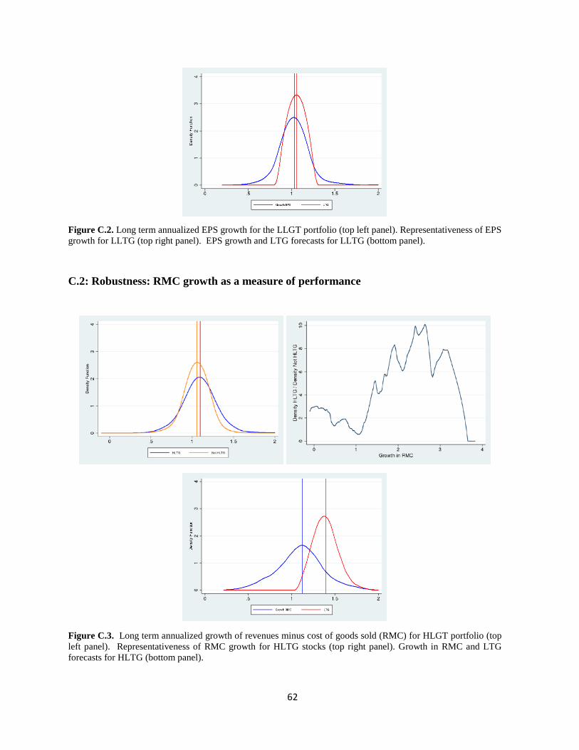
62

Figure C.2. Long term annualized EPS growth for the LLGT portfolio (top left panel). Representativeness of EPS growth for LLTG (top right panel). EPS growth and LTG forecasts for LLTG (bottom panel).

C.2: Robustness: RMC growth as a measure of performance

Figure C.3. Long term annualized growth of revenues minus cost of goods sold (RMC) for HLGT portfolio (top left panel). Representativeness of RMC growth for HLTG stocks (top right panel). Growth in RMC and LTG forecasts for HLTG (bottom panel).

63

D. Coibion and Gorodnichenko Analysis

D.1 Overreaction to News vs Adaptive Expectations

Adaptive expectations (Equation 11) predict no over-reaction to news after the persistence

of the earnings process is accounted for. From (11), the forecast error on an AR(1) process with

persistence 𝜌𝜌 is 𝑥𝑥𝑡𝑡+1 − 𝑥𝑥𝑡𝑡+1𝑎𝑎 = (𝜌𝜌 − 1)𝑥𝑥𝑡𝑡 + �1−𝜇𝜇𝜇𝜇� (𝑥𝑥𝑡𝑡+1𝑎𝑎 − 𝑥𝑥𝑡𝑡𝑎𝑎). Controlling for 𝑥𝑥𝑡𝑡 fully accounts

for mechanical over-reaction in processes with low persistence. The adaptive forecast revision

(𝑥𝑥𝑡𝑡+1𝑎𝑎 − 𝑥𝑥𝑡𝑡𝑎𝑎) should positively predict forecast errors as in the under-reaction models. This

prediction is not shared by our model because diagnostic expectations over-react to news

regardless of the persistence of the data generating process. Table C.1 reports the results. The

coefficients on forecast revision become larger than those estimated in Table 2, but they remain

mostly negative and statistically significant.

Table D.1: Forecast Errors

Each entry in the table corresponds to the estimated coefficient of the forecast errors (epst+n/ epst)1/n-LTGt for n=3, 4, and 5 on the variables listed in the first column of the table as well as (log) epst and year fixed-effects (not shown).

Dependent Variable

(epst+3 / epst)1/3-LTGt (epst+4 / epst)1/4-LTGt (epst+5 / epst)1/5-LTGt LTGt-LTGt-1 0.0332 -0.0733 -0.1372b (0.0725) (0.0660) (0.0589) LTGt-LTGt-2 -0.0875 -0.1435b -0.1842a (0.0641) (0.0691) (0.0545) LTGt-LTGt-3 -0.0956 -0.1184c -0.1701a (0.0578) (0.0627) (0.0517)

64

D.2 Underreaction for forecasts at short time horizons

Table D.2 tests the predictability of forecast errors in the forecast of earnings levels, as opposed to the predictability of errors in LTG forecasts analysed in Table 2. The results suggest underreaction for forecasts at short time horizons (i.e. one year ahead), compatible with Bouchaud et al. (2016). As in Table 2, as the forecasting horizon increases to three years ahead, the coefficient becomes less positive and even negative in some specifications.

Table D.2: EPS Forecast Errors at short time horizons

Each entry in the table corresponds to the estimated coefficient of the forecast errors for t+1, t+3, and t+5 on the variables listed in the first column of the table as well as year fixed-effects (not shown). All forecast errors are scaled by lagged sales per share.

(epst+1-Etepst+1) / spst-1 (epst+3-Etepst+3) / spst-1 (epst+5-Etepst+2*(1+LTGt)

3) / spst-1

LTGt-LTGt-1 0.0839 -0.3226b -0.5918a (0.0554) (0.1312) (0.1435) LTGt-LTGt-2 0.1629a 0.1262c -0.0227 (0.0275) (0.0677) (0.0772) LTGt-LTGt-3 0.0825a -0.0664 -0.2145b (0.0195) (0.0532) (0.0919)

D.3 Overreaction and predictable returns

We next try to tie over-reaction to news to the return spread between HLTG and LLTG

portfolios. We estimate Equation (10) by pooling firms at the industry level, using the Fama and

French classification. To capture industry and firm specific factors, we allow for industry×year

fixed effects. This yields an industry level estimate 𝛾𝛾𝑠𝑠, where 𝑠𝑠 indexes the industry, which we can

correlate with the industry level LLTG-HLTG spread. These results should be taken with caution,

due to the small number of industries.

65

In Figure D.1, we compare the post formation return spread across different terciles of the

distribution of industry 𝛾𝛾𝑠𝑠. Consistent with our prediction, the extra return obtained by betting

against HLTG firms is highest in sectors that feature most over-reaction, namely those in the

bottom tercile of 𝛾𝛾𝑠𝑠. The return differential is sizable, though given the small sample size it is not

statistically significant. Thus, the pattern of LLTG-HLTG return spreads across industries is

consistent with a link from overreaction to news to overvaluation of HLTG stocks and thus to

abnormally low returns of the HLTG portfolio.

Figure D.1. Overreaction and return spread across industries. For each of the 48 Fama-French industries, we estimate the regression: (𝐸𝐸𝑃𝑃𝑆𝑆𝑡𝑡+4/𝐸𝐸𝑃𝑃𝑆𝑆𝑡𝑡)1/4 − (1 + 𝐿𝐿𝑇𝑇𝐺𝐺𝑡𝑡) = 𝛼𝛼𝑖𝑖 + 𝜇𝜇𝑖𝑖,𝑡𝑡 + 𝛾𝛾𝑖𝑖(𝐿𝐿𝑇𝑇𝐺𝐺𝑡𝑡 − 𝐿𝐿𝑇𝑇𝐺𝐺𝑡𝑡−3) + 𝜀𝜀𝑖𝑖,𝑡𝑡 where μt are year fixed effects, EPS is earnings per share, and LTG is the forecast long-term growth in earnings. We rank industries according to 𝛾𝛾𝑖𝑖𝑖𝑖 and form the following three groups: (1) 14 industries with the lowest 𝛾𝛾𝑖𝑖𝑖𝑖, (2) 24 industries with intermediate values of 𝛾𝛾𝑖𝑖𝑖𝑖, and (3) 14 industries with the highest 𝛾𝛾𝑖𝑖𝑖𝑖. Finally, for each year and each group, we compute the difference in return for the LLTG (i.e. bottom 30% of LTG) and HLTG (i.e. highest 30% of LTG) portfolios. The graph shows the arithmetic mean of the LLTG-HLTG spread for grouping industries based on 𝛾𝛾𝑖𝑖𝑖𝑖 from the regression.

66

E. Calibration

In this section, we extend our analysis of the calibration with two numerical exercises. The

first tests the robustness of our estimate 𝜃𝜃 = 1.2. To do so, we evaluate the matching between the

predicted return spread and the empirical return spread for 𝜃𝜃 ∈ [0,2.4] (keeping the other

parameters constant). Figure D.1 below shows that the match is indeed optimized for 𝜃𝜃 = 1.2 and

that it drops fast as 𝜃𝜃 departs from this value.

Figure E.1. For �𝑎𝑎, 𝑏𝑏,𝜎𝜎𝜂𝜂,𝜎𝜎𝜖𝜖� = (0.9,0.33,0.15,0.17), as given by our calibration, and each 𝜃𝜃 ∈ [0,2.4] we compute the LLTG-HLTG return spread (𝑠𝑠𝑝𝑝𝑣𝑣𝑒𝑒𝑎𝑎𝑢𝑢𝜃𝜃). The figure plots the absolute distance �𝑠𝑠𝑝𝑝𝑣𝑣𝑒𝑒𝑎𝑎𝑢𝑢𝜃𝜃 − 𝑠𝑠𝑝𝑝𝑣𝑣𝑒𝑒𝑎𝑎𝑢𝑢����������� where 𝑠𝑠𝑝𝑝𝑣𝑣𝑒𝑒𝑎𝑎𝑢𝑢���������� = 12.5% is the empirically measured return spread.

The second exercise is to confirm numerically the pattern of Figure 9, namely that high

LTG forecasts are on average revised downwards, even conditional on positive news, that is,

earnings that exceeded (distorted) expectations. Figure D.2 below plots the equivalent of Figure

10 for our calibration.

67

Figure E.2. For each period 𝑡𝑡 and each firm in the 𝐻𝐻𝐿𝐿𝑇𝑇𝐺𝐺𝑡𝑡 and 𝐿𝐿𝐿𝐿𝑇𝑇𝐺𝐺𝑡𝑡 portfolios, we compute the surprise ln𝐸𝐸𝑃𝑃𝑆𝑆𝑡𝑡+1 − ln𝐸𝐸𝑃𝑃𝑆𝑆𝑡𝑡 − 𝐿𝐿𝑇𝑇𝐺𝐺𝑡𝑡. Pooling the data for all 𝑡𝑡 and both portfolios, we rank the surprises in deciles and plot the average revision of 𝐿𝐿𝑇𝑇𝐺𝐺 for each portfolio in each decile.

In the model, news and forecast revisions are positively correlated. Crucially, however,

they may go in opposite directions. For a range of positive surprises – namely, realized growth

above the diagnostic forecasts – forecasts about HLTG firms are still revised downwards.

Naturally, for sufficiently large positive surprises (larger than 1.5𝜎𝜎𝜖𝜖, in our calibration) forecast

revisions are positive. The converse holds for LLTG.