the impact of growth on distribution of income across ... the impact... · the impact of growth on...
TRANSCRIPT
16th International Input-Output Conference, Istanbul, Turkey, 2-6 July 2007
1
The Impact of Growth on Distribution of Income across Ethnic Groups: a
Social Accounting Matrix (SAM) Approach
M. Yusof Saari*, Erik Dietzenbacher** and Bart Los***
*SOM Research School, University of Groningen, PO Box 800, 9700 AV Groningen, the
Netherlands. Email: [email protected]
**Faculty of Economics, University of Groningen, PO Box 800, 9700 AV Groningen, the
Netherlands. Email: [email protected]
***Faculty of Economics, University of Groningen, PO Box 800, 9700 AV Groningen, the
Netherlands. Email: [email protected]
Abstract
The present paper examines the impact of growth estimated in the Ninth Malaysia Plan on
the distribution of income among various ethnic groups across regions by employing two
types of SAM models. Besides typical approach of Pyatt and Round (1979), we provide an
alternative approach by treating government as an endogenous in the model of multiplier.
The latter approach however has to be modified by adopting a mixed endogenous-
exogenous SAM multiplier for ensuring demand and supply derived are internally
consistent. We find that both models show the growth has significant impact in improving
the distribution of income especially to enhance income of low-income group. By
introducing government sector into the model, the income inequality among ethnics
reduced significantly by generating a large income effect through the inter-dependency
effect. We are also observe that source of inter-ethnic inequality in the economy is largely
explained by unbalancing in labour structure.
Keywords: Social Accounting Matrix (SAM), growth, income distribution, multiplier
decomposition
16th International Input-Output Conference, Istanbul, Turkey, 2-6 July 2007
2
1. Introduction
Study on the impact of growth on distribution of income had been widely covered in the
literature. Studied by Adelman and Morris (1973) and Adelman and Robinson (1978) for
instances had shown high growth rate tended to shift the income distribution in favour of a
high-income group and against low-income group. As a consequence, distribution of
income between the high-income and low-income groups deteriorated. Economic growth
alone however is neither necessary nor sufficient for reducing poverty. Tanzi (1998) and
Shari (2000) suggested that economic growth was necessary for poverty alleviation but it
may not be sufficient to improve distribution of income. It is also clear that distributional
issue has contributed to increase social tensions and created difficult policy choices for
policy maker especially for multi-racial society. According to Thorbecke and Charumilind
(2000) inequality in distribution of income is the crucial factor leading to social conflict and
political instability. Empirical evidences revealed that income inequality had significant
impact to the country’s political stability and social conflicts i.e. riot and revolution as
documented by Nagel (1974) and Muller (1988a,b).
Similarly, as a pluralistic1 developing country, income inequality in Malaysia is not
a new issue since it had been raised in the past four decades ago when the ethnic riot was
took place in 1969. The 1969 riot highlighted the dangers inherent in the multi-racial
society when ethnic prejudices are exacerbated by the economic disparities. Consequently,
economic development policies in Malaysia since 1970 are being shaped by the
government commitment to ensure that benefits of economic growth are equitably shared
among all Malaysians. This commitment is built upon the realization that greater equity in
the distribution of income and opportunities for wealth creation is essential for sustained
economic growth as well as for the maintenance of social stability and national unity.
1 The major ethnic groups in Malaysia comprise of the Malay (indigenous), Chinese and Indian. The composition of the Malaysian population shows that Malay is the dominant group (51 per cent), followed by Chinese (31 per cent), Indian (10 per cent) and Others (8 per cent)

16th International Input-Output Conference, Istanbul, Turkey, 2-6 July 2007
3
Recently, under the current Ninth Malaysia Plan (2006-2010), the government will
continue to pursue a development policy that emphasizes growth with distribution.
Accordingly, distribution policies, programmes and projects will be better designed and
carefully monitored in order to achieve greater economic growth as well as greater equality
of income among all ethnic groups. With 6.0 per cent of annual growth rates estimates in
the Ninth Malaysia Plan, one obvious question continues to be raised: how are the fruits of
growth distributed equally across all Malaysians? Test of this empirical question is the
subject of our study.
In addressing this issue, we shall examine the impact of growth estimates in the
Ninth Malaysia Plan on distribution of income among major ethnic groups across regions
by using a Social Accounting Matrix (SAM) model. The advantage of this approach is it
provides a comprehensive framework, incorporating elements of growth and income
distribution into one coherent accounting framework. In fact, most of the construction of
SAMs in the developing countries were provided data framework for the quantitative
analysis of combating poverty and income distribution. Therefore, for the purpose of this
study, the SAM for Malaysia with special references to income distribution among various
ethnic groups across regions is constructed.
There are two types of SAM models are applied. Besides typical approach of Pyatt
and Round (1979), we provide an alternative approach by treating government as an
endogenous component together with production, factor, household and company accounts.
By introducing government as an endogenous account in the model of multipliers, we can
capture the redistribution income effect through the instrument controlled by the
government such as public expenditure and taxation. We however modify the latter
approach by adopting a mixed endogenous-exogenous SAM multiplier in order to ensure
demand or injection and supply or leakages derived are internally consistent. On the other
hand, by decomposing SAM multiplier, we can simply examine the role of government in
affecting distribution of income through the distributional and inter-dependency effects.
The distributional is further decomposed into industrial, direct and transfer effects.

16th International Input-Output Conference, Istanbul, Turkey, 2-6 July 2007
4
This paper is organised as follows; Section 2 briefly reviews growth performance
and patterns of distribution of income achieved during the 1970-2002 period. Section 3
discusses in general, the source of growth estimates in the Ninth Malaysia Plan from
demand side. Section 4 describes the general structure of the Malaysian SAM and its details
disaggregation for the household, factor and production sectors. Section 5 outlines the
analytical SAM framework associated in the study. Section 6 presents the result of the
impact of sectoral growth on the distribution of income. Concluding remarks follow in
section 7.
2. Economic Growth and Distribution, 1970-2002
Over the 1970-1990 period, the economy grew by an average rate of 6.7 per cent per
annum. The growth was accompanied by considerable transformation of structure of the
economy from resource based economic activities to non-resource based industrial
activities, led by the expansion in the manufacturing sector. This sector grew annually by
10.3 per cent resulted in its share to the Gross Domestic Product (GDP) raised from 13.9
per cent in 1970 to 27 per cent in 1990. With higher growth rates in the manufacturing
sector, share of the agriculture sector declined from 29 per cent in 1970 to 18.7 per cent in
1990. The high growth rate of the Malaysian economy during this period was a result of
successfully implementation of the New Economic Policy (NEP). This policy was guided
by the strategy of growth with distribution, and twin-pronged objectives of the eradication
of poverty irrespective of race and the restructuring of society to correct the identification
of race with economic function2.
The growth and structural transformation of the economy during the NEP period
had interesting implications to the income distribution pattern of all Malaysians. The gap in
2Identification of ethnic with economic function existed as a result of colonial labour policy of ‘divide and order’, introduced by British (1786-1942). When British took over Malaysia (Malaya), Chinese and Indian were put in the commercial and industrial activities areas and engaged in the high productivity modern sector whereas Malay were located in the Malay Belt and engaged in the low productivity traditional sector of peasant agriculture and fishing. Malay were only allowed to involve in the modern sector as civil servant i.e. police and military where the non-Malays were not attracted as income received from this sector was relatively low compare to the other modern sectors.

16th International Input-Output Conference, Istanbul, Turkey, 2-6 July 2007
5
ethnic community incomes narrowed significantly and the size of distribution of income
has become more equal during the NEP period. As shown in Table 1, mean income of
Bumiputera3 increased significantly from MR 172 in 1970 to MR 940 in 1990 with
registered the highest growth rate compared to other ethnics by 8.9 per cent per annum. As
a consequence, income inequality between Bumiputera-Chinese narrowed from 1:2.29 to
1:1.74 while Bumiputera-Indian improved from 1:1.77 to 1:1.29, respectively. Similarly,
income gap between rural and urban reduced from 1:2.14 to 1:1.67.
During the 1990-2002 period, the economy was driven by the New Development
Policy (NDP). The NDP seeks to maximise economic growth through policy that allow for
free play of market mechanism and the active participation of the private sector. The
implication of these liberalisation policies to the nation growth that the economy grew by
an average rate of 7.0 per cent per annum higher than the NEP achievement with strong
recovery in the demand of manufacturing products especially electric and electronics sub-
sector. The growth of the manufacturing sector was accompanied by expansion in the
export-oriented industries as well as greater diversification of its market. To support the
expansion of the manufacturing sector, the government took steps to develop the services
sector to be a new source of growth. This sector grew by an average rate of 8.3 per cent per
annum. However, the agriculture which traditionally provided the impetus growth to the
economy was continuously declined by 0.5 per cent per annum.
<Table 1>
The consequence of liberalisation and deregulation policies had different
implication on growth and income distribution. Even though Malaysia has experienced
catch-up rapid economic growth during the 1990-2002 period, income distribution patterns
among ethnic groups and regions were deteriorated. While mean household incomes were
3Bumiputera which translated literally means son of the soil, is an official definition widely used in Malaysia, embracing Malay and other indigenous groups in the Peninsular Malaysia and the tribal peoples of the East Malaysia. On average, Malay constitutes 80 per cent of total Bumiputera population while the rest of 20 per cent is other indigenous groups

16th International Input-Output Conference, Istanbul, Turkey, 2-6 July 2007
6
increasing for all ethnic groups as well as both rural and urban areas, the differential rates
of income growth among them resulted in an increase in inequality. The growth rate of
Bumiputera’s income (8.0 per cent) is not only lower than Chinese and identical with
Indian, but also lower than the growth rate of income that had been achieved by them
during the NEP period. In 2002, mean income of Bumiputera constituted only 56 per cent
of mean income of Chinese and 78 per cent of mean income of Indian. As a consequence,
income inequality among Bumiputera, Chinese and Indian increased during the 1990-2002
period. Similarly, the differential in income growth between rural and urban household
resulted in an increase in rural-urban inequality i.e. from 1:1.67 in 1990 to 1:2.11 in 2002.
Although economic growth has been a driving force for raising income and living
standards, it does not by itself ensure that benefits of growth are equitably shared among all
in society. Liberalisation of the economy by promoting high growth rates and rapid
industrialisation tend to shift the income distribution in favour of the high-income group
and deteriorated the low-income group i.e. Bumiputera. Besides economic liberalisation,
supply side policies such as continuing to influx of migrant worker; limited expansion of
flexible social corporatism; and declined in the agricultural sector which has made it lag
behind other sectors are the another factors why the unfavourable trend in income
distribution (Shari, 2000).
3. Source of Growth
Approaching the plan from demand side, the Economic Planning Unit (EPU) provides the
estimated Gross Domestic Product (GDP) by category of demands for year 2005 and 2010.
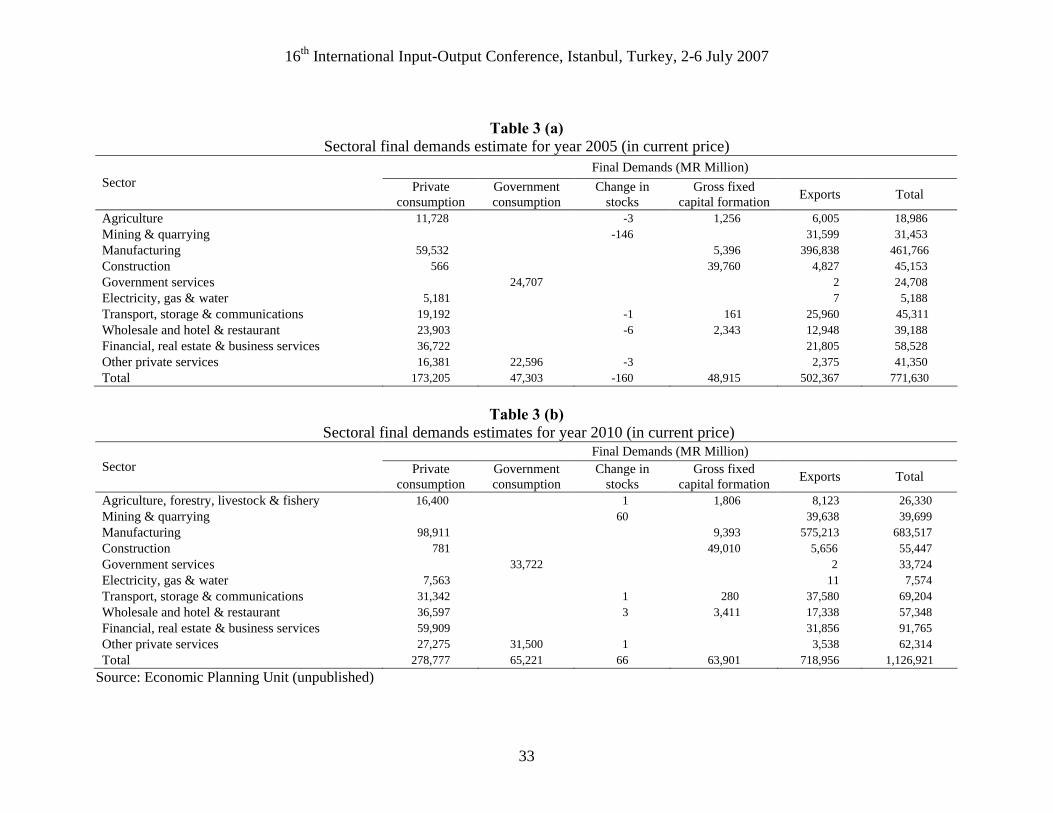
While Table 2 shows an aggregate demand, Table 3 (a) and (b) present sectoral demands
estimates in year 2005 and 2010, respectively. Notice that figures in Table 2 show total
demands which comprise of both domestic and import commodities whereas Table 3 (a)
and (b) reflect only demand on domestic commodities.
<Table 2>
16th International Input-Output Conference, Istanbul, Turkey, 2-6 July 2007
7
<Table 3(a)>
<Table 3(b)>
During the plan period, the Malaysian economy is projected to grow by 6.0 per cent
per annum in real terms. The growth will be supported by domestic demand with strong
recovery in private expenditure - investment and consumption. Private expenditure will
continue to be the driving force of the economy, consistent with the overall policy of
encouraging the private sector to spearhead economic growth. Private investment in the
form of gross fixed capital formation is projected to grow by 11.2 per cent per annum and
its share to the total investment is expected to be 51 per cent in year 2010. The rest of 49
per cent of investment will be contributed by the public sector (Economic Planning Unit,
2006). Sectorally, as shown in Table 3 (b), 76.7 per cent of the sectoral investment is
expected to be invested in construction, 14.7 per cent in manufacturing, 5.8 per cent in
services, and 2.8 per cent in agriculture.
With 6.9 per cent annual growth rate, private consumption is expected to be the
second sources of growth of the domestic economy during the plan period. The growth in
private consumption is expected as a result of an increase in household disposable income
and continuing improvement in consumer confidence underpinned by sustained
employment growth and favourable commodity prices. As revealed in Table 3 (b), demand
on the services commodities is projected to contribute a large share of the domestic private
consumption which recorded at 58.4 per cent. Demand from this sector is expected to be
strongly supported by demand of financial, real estate & business services; wholesale &
retail trade and hotel & restaurants; and transport, storage & communications commodities.
On the other hand, with 10.7 per cent of annual growth rate higher than services sector (9.9
per cent) between 2005 and 2010, demand of the manufacturing commodities is expected to
contribute significantly to the growth of private consumption patterns. For public
consumption, it is projected to grow by 5.3 per cent per annum, and will contribute about
12 per cent to the GDP in year 2010.

16th International Input-Output Conference, Istanbul, Turkey, 2-6 July 2007
8
In terms of external demand, an export of commodities is projected to grow by 7.1
per cent per annum as a result of improving competitiveness and better prospects in world
trade. Export of manufacturing commodities is projected to contribute 80 per cent of
sectoral exports which will expand by 8.2 per cent per annum (2005-2010). The high
growth rate of manufacturing exports reflects the sustained expansion in demand from
traditional countries i.e. America, Middle East and ASEAN, as well as non-traditional
markets such as China, India and Western Europe. Export from services sector on the other
hand is estimated to contribute 12.6 per cent of sectoral exports which largely demanded
from the transport, storage & communication; and financial, real estate & business services
commodities. The increasing usage of cellular and its related services, expansion of
international trade and travel agency, and effort of placing Malaysia as an emerging
advanced financial market are expected to be the major factors in contributing exports of
these sub-sectors. Exports of the mining & quarrying commodity is expected to contribute
5.5 per cent of total sectoral exports which mainly driven by exports of crude oil. The share
of agriculture commodity to the sectoral exports is expected to contribute 1.9 per cent
during the plan period which is mostly contributed by the positive growth in the export of
rubber, palm oil, cocoa and forestry commodities. To support the anticipated growth of the
export especially the manufacturing sector, imports of commodities are estimated to grow
by 7.9 per cent per annum, largely supported by import of intermediate commodities.
Overall, the sectoral demand in the Ninth Malaysia Plan as depicted in Table 3 (b)
reveals that the structure of demand in the Malaysian economy is largely supported by
demand from the manufacturing commodity – followed by services, construction, mining &
quarrying, and agriculture commodities. Demand of the manufacturing commodity is
expected to contribute 60.7 per cent to the sectoral demand in year 2010 which 84.2 per
cent from its total demand contributed by export. Unlike the manufacturing sector, 50.5 per
cent of total demand from services sector is largely demanded by private consumption and
only 21.4 per cent by exports. Therefore, it is strongly infers that the economic activities in
the year 2010 influenced significantly by the manufacturing sectoral linkages effect due to
the highest sectoral demand is attributed from this sector than other sectors.
16th International Input-Output Conference, Istanbul, Turkey, 2-6 July 2007
9
4. The Social Accounting Matrix for Malaysia
Development of an SAM in Malaysia can be traced as far back in 1978 when the first SAM
was developed for the 1970 database. In collaboration with the government of Malaysia,
the World Bank experts, Pyatt and Round (1984) constructed a large SAM which
distinguished between national and regional SAM. They had done a great work to improve
the macroeconomic data base for Malaysia in calendar year 1970. Based on the 1970
Malaysian SAM, several modifications suit to the purpose of the present study shall be
made. Basic assumptions of analysis regarding to household sectors are: (i) household
income by regions and ethnic groups is based on structure of income provided by the
household income surveys (HIS), (ii) household expenditure by regions and ethnic groups
is based on structure of expenditure available in the household expenditure surveys (HES),
and (iii) production structure is based on the 2000 input-output table. In fact, year 2000 was
selected as a baseline data for constructing SAM because the latest input-output table
published by the Department of Statistics (2005) is 2000 base-year.
4.1 General Structure
A square matrix of accounting structure underlying the aggregative accounts for Malaysian
SAM is presented in Table 4. In the SAM, incomings are indicated as receipts for the row
(i) in which they are located while outgoings are indicated as expenditure for their column
(j). The corresponding row and column totals of the matrix must be equal, consistent with
the fundamental law of economics that for every income there is a corresponding outlay or
expenditure. The major components of SAM accounts comprises factor of production,
institutions (household, company and government), production activities, consolidated
capital, current and capital for rest of the world and indirect tax. Factor of production,
production activities and household sectors are disaggregated into 27, 92 and 9 categories,
respectively, while the rest of the remaining accounts in the SAM are in the aggregate form.
Thus, the total sum of all accounts in our SAM contains 134 x 134 dimensions of matrix.
16th International Input-Output Conference, Istanbul, Turkey, 2-6 July 2007
10
<Table 4>
In this study, the SAM is constructed by using a top-down approach. Specifically,
before estimating in details of the 134 by 134 accounts in the SAM, a highly aggregated
SAM based on the country’s national account statistics is built. To be more precisely, the 9
by 9 matrix of aggregate SAM is prepared first. Then, this value reacts as control value
when detailed accounts of each sector in the SAM particularly household and factor
accounts are estimated. Multi-purpose survey i.e. household income survey and household
expenditure survey are used to construct detail accounts of the particular accounts
Table 4 shows also the relationships among sectors in the economy within the single
accounting framework. We can trace the distribution of income from production sector to
household by looking at the flows around the SAM. The mapping of distribution of income
from production to household can be traced through three distributional mechanisms: (i) the
structure of production activities, (ii) factorial distribution of value added from production,
and (iii) distribution of institutional incomes i.e. household and company from factor
market. Referring to the intersection between first row and second column of Table 4, it can
be observed that the factorial income received by the various categories of labours and
capitals from the production activities. Besides requiring the intermediate input from other
production activities, production also consumes the primary input supplied by factors of
production in the form of labour and capital. By providing factor services to production
activities, labour receives payments in the form of compensation of employees4 while
capital receives operating surplus 5 , depending on the level of endowment in the
technological process. Then, from the total amount of income received by factors, they
distribute to the various categories of household and company as shown in the intersection
4Compensation of an employee includes remuneration, in cash or in kind, payable by the production activities
to employee in return for work done during the accounting period. The components of compensation of employees comprise of wages and salaries, allowances and other payments received in kind.
5Operating surplus measures the surplus accruing from production before taking account of any interest, rent or similar charges payable on financial or tangible non-produced assets borrowed or rented or owned by enterprise (company) and unincorporated enterprise (households)

16th International Input-Output Conference, Istanbul, Turkey, 2-6 July 2007
11
between third and fourth rows, and first column of Table 4. This mapping is essentially to
determine the distribution of wealth in the economy. Household receives income in the
forms of compensation of employee and unincorporated business profit while company
receives corporate business profit.
4.2 Disaggregation for Income Distribution Analysis
For the purpose of studying the distribution of income, the most important disaggregation is
that of the household sector. Such a disaggregation is crucial in order to capture how
changes in the production structures are transmitted to household through the factor market.
The first distinction of household is made between citizen and non-citizen of Malaysian
household. It is important to distinguish citizenship categories since recently, the number of
foreign workers influenced significantly to the labour force which grew by 18.8 per cent
per annum within 2000-2005 (Economic Planning Unit, 2006). Most of them are the
Indonesian, Bangladeshi and Filipinos which engaged in the plantation and agriculture, and
manufacturing sectors. The, the citizenship household is further disaggregated into several
classifications.
The classification of citizenship household adopted here is centered on
socioeconomic groups rather than by income levels as explained by Pyatt and Thorbecke
(1976). As the pluralistic country, it is considered important to distinguish four major
ethnic groups throughout the household sector – Malay, Chinese, Indian and Others6. In
addition, those disaggregations are important since the recent government’s development
strategy include specific concerns for the distribution of income between the various ethnic
groups. Besides focusing on income distribution between ethnicity, we also capture
regional differences by disaggregating them into rural and urban areas. The regional
criterion for disaggregation is useful since the urban and rural distinction captures many
aspects of duality. Depending on this distinction, households with otherwise similar
characteristics are quite likely to be paid different wages and generally to be subject to
6 The others groups comprise of dozens of minority ethnic groups which are mostly located in the East Malaysia. These minority groups include for instance Iban, Kadazan, Bajau, Murut, Suluk and etc.

16th International Input-Output Conference, Istanbul, Turkey, 2-6 July 2007
12
different sets of socio-economic behaviour. Table 5 summarizes details disaggregation of
the nine categories of households in the SAM frame.
<Table 5>
Factor of production is distinguished between labour and capital. The former is
further disaggregated into 25 categories of labours according to their citizenship status,
region, ethnic group and education level as shown in Table 5. These aggregations are
similar with respect to location and race of household except for education level. The
education criterion7 which complements location and race in defining labour types turns out
to be important in explaining income differences. Assuming labours are homogenous
irrespective ethnic groups, the wage rate received by labours from the production activities
in which sector their employed are totally depend on education level. On the other hand,
capital input is further distinguished between household and company in the form of
unincorporated business profit and corporate business profit, respectively.
Another important sector in the SAM framework is production activities. Based on
the 2000 input-output table published by Department of Statistics (2005), we take into
account 92 production activities starting from agriculture sector to services sector. The
2000 input-output table was compiled by using new industrial classification, Malaysian
Standard Industrial Classification (MSIC), following the latest International Standard
Classification of All Economic Activities (ISIC). The rest of the remaining accounts in the
SAM are in aggregate form.
4.3 Aggregation of the SAM
Following the macro planning framework in the Ninth Malaysia Plan, our analytical
framework requires the production activities in the SAM frame to be aggregated into ten
broad sectors. This aggregation need to be done because in the Ninth Malaysia Plan, the 7Education criterion is based on certificate obtained at school, college and university. Those who are did not have formal education and primary school certificate are categorised under none education category while L.C.E., M.C.E. and H.S.C. certificates are categorised under secondary education, and diploma, and degree (or above) certificates are considered as tertiary education.
16th International Input-Output Conference, Istanbul, Turkey, 2-6 July 2007
13
EPU has provided only the estimates demand for the broad sector categories and there is no
information available for the details sectors. Thus, our aggregated SAM version contains 52
by 52 matrix dimensions, reducing the production sector from 92 to 10 sectors.
5. SAM Modelling for Income Distribution
5.1 The Impact of Sectoral Growth on Household Income
The SAM framework is a useful starting point for economy wide analysis, which focuses
on the demand side. By deriving multiplier, it can be used similarly with the obvious input-
output model, but the difference that the SAM contains more variables and relationships. If
a certain number of conditions are met – (i) the existence of excess capacity which would
allow prices to remain constant, (ii) constant expenditure propensities of endogenous
account and (iii) production technology and resource endowment are given, the SAM
multipliers can be used to evaluate the potential impacts of demand changes on household
groups by ethnics and regions. However, before deriving the SAM multipliers, it is
important to understand the underlying methodology, determining the endogenous and
exogenous accounts from the nine SAM accounts. The choice regarding subdivision into
endogenous and exogenous accounts can be lengthy discussions on the logic and
operational in the planning framework. Following the typical approach of Pyatt and Round
(1979), production, factor, household and company are considered as endogenous accounts
while the rest of the remaining accounts (government, consolidated capital, rest of the
world and indirect tax) is considered exogenous. As a result of this manipulation, an
economy-wide model in the form of Table 6 is produced.
<Table 6>
Determination of the endogenous accounts from the accounting relationship can be
expressed in equation (1).
y = Ay + x (1)
From Table 4, matrix A in equation (1) can be partitioned as;

16th International Input-Output Conference, Istanbul, Turkey, 2-6 July 2007
14
0 A12 0 A = 0 A22 A23 (2) A31 0 A33
Then, from equation (1), income for endogenous account simply can be obtained via the
following expression;
y = (I – A)-1x = Mx (3)
where I is an identity matrix, A is (n x n) sub-matrices containing an average expenditure
propensities, showing the income of endogenous account i received from endogenous
account j as a proportion of the expenditure of endogenous account j. These average
expenditure propensities can be derived simply by dividing a particular element in any of
the endogenous accounts by the total income for the column account in which the element
occurs. M is a (n x n) matrix of multiplier and x is a (n x m) vector of demand. Specifically,
equation (3) indicates that endogenous income of y (factorial incomes, y1; production
incomes, y2; household incomes, y3; and company incomes, y4) can be derived by
multiplying injection, x by the multiplier matrix of M. It can be used to calculate the
endogenous incomes associated with any given changes in demand (injection) of any
production sectors. It captures both the Leontief production linkages and the consumption
expenditure linkages induced by changes in production activities through their effect on
household incomes.
Analytically, the estimated final demand components of private and government
consumption, investment (gross fixed capital formation and change in stock), and exports
for year 2005 and 2010 will be our exogenous variables. However, for analysis purpose, we
only take into account the effect of investment, government consumption and exports as
household (private) consumption is now treated as an endogenous sector that will interact
in the economic system. Specifically, we can define the exogenous demand as,
y = (I – A)-1x = M (xg + xi + xe) (4)

16th International Input-Output Conference, Istanbul, Turkey, 2-6 July 2007
15
Besides the above conventional criterion, we modify also the multiplier matrix in
equation (3) by treating government as an endogenous component together with production,
factor, household and company. The rest of the remaining accounts of consolidated capital,
the rest of the world and indirect taxes are treated as exogenous accounts. By introducing
government as an endogenous account in the model of multipliers, the redistribution
income effect to household through public expenditure and public taxation when the
government receives exogenous incomes can be captured. In particular, it can extent our
knowledge of income distribution effects due to variables controlled by public institutions,
such as taxes and transfers (Llop and Manresa, 2004). Hence, this alternative approach can
be expressed via the following equation;
y = (I - A*)-1x = M*x (5)
where A* and M* are (n+1 x n+1) sub-matrices containing the average expenditure
propensities of endogenous accounts and (n+1 x n+1) matrix of multiplier derived after
endogenousing government sector, respectively. Nevertheless, equation (5) cannot be
directly applied in this study as supply (leakage) derived is not internally consistent with
demand (injection). Inconsistency exists because besides treating government as an
endogenous sector, its also considered as exogenous component together with investment
and exports. Therefore, in addressing this issue, we employ a mixed type of SAM model -
combination of endogenous-exogenous variables as applied from Miller and Blair (1985).
Applying of this approach, output of government sector (revenue) will be treated as
exogenous variable in the model. Specifically, output of government can be obtained
indirectly from equation (4) as proportion of each endogenous variables (factor, production,
household and company) which leaks out as expenditure into government sector in the form
of direct and indirect taxes. This calculation is represented by equation (6)
ŷg = g (I – A)-1x = g’Mx (6)
where g is a (1 x n) vector of average propensities leak by government sector. Taking the
effect of government output as an exogenous, equation (5) therefore can be modified as

16th International Input-Output Conference, Istanbul, Turkey, 2-6 July 2007
16
y = (I – Ag)-1x* = Mg (x*i + x*e) (7)
where matrix Mg is modified from original matrix M* which contains mixed element of
endogenous-exogenous variables and x*’s comprises of existing and the new level of
demands generated as a result of an increase in output of government. Detail description of
this approach can be referred in an Appendix.
5.2 Decomposition of SAM Multiplier
Conceptually, the size of multiplier of M* is larger than M because it contains an additional
endogenous variables of government sector while not for the former. Accordingly,
household income generated by using the latter approach is greater than the former despite
the level of demand applied in the latter approach is relatively lower than the former.
However, one important question continues to be raised; does the government intervention
gives more benefits to the low-income group in terms of income generation. If true, in what
way it has improved income of this group. To understand the various mechanisms and
linkages within the SAM frame, we can extent our analysis by conducting the multiplier
decomposition technique. According to Pyatt and Round (1979), matrix of multiplier M (as
well as M*) can be decomposed into three separate effects of (i) transfer effect – captures
the effect of transfers within the economy i.e. transfers of income among production sector
or among institutions, (ii) open loop effect – captures the cross-effects of multiplier process
whereby an injection into one part of the system has repercussions on the other parts, and
(iii) closed loop effect – captures full circular effects of an income injection going round
the system and back to its point of origin in a series of repeated. According to this approach,
matrix of multiplier M now can be decomposed as follows;
M = M3M2M1 (8)
where, M1, M2 and M3 represent transfer effect, open loop effect and closed loop effect,
respectively. Specifically, M1, M2 and M3 can be derived as;
M1 = (I - Ā)-1; M2 = (I + A* + A*2); M3 = (I - A*3)-1 (9)
16th International Input-Output Conference, Istanbul, Turkey, 2-6 July 2007
17
By partitioning the matrix of A* and Ā, element of A*ij and Āij can be defined by the
following equations;
0 0 0 0 A*12 0Ā = 0 A22 0 and A* = 0 0 A*23 (10) 0 0 A33 A*31 0 0
where; A*12 = A12; A*23 = (I - A)-1A23; A*31 = (I - A)-1A31 (11)
In addition to the above specification, we attempt to decompose the multiplier M into two
separate effects, the distributional effects and interdependency effects as proposed by
Thorbecke and Jung (1996) which can be shown in equation (12).
M = R.D (12)
The distributional effects in addition can be further decomposed into three effects; (i)
transfer effect – incomes accruing to the institutions from transfer and remittances from
other institutions, (ii) direct distributional effect - translation from the factorial income
distribution to the distribution of income of different household groups, depending on
which groups own the factors, and (iii) industrial effect – inter-linkages among production
sectors which represented by the input-output relation. Thus, the distributional effect can be
derived as;
D = (I - A33)-1A31A12 (I - A22)
-1 (13)
where the D3 (m x m) = (I - A33)-1 represents the transfer effect, D2 (m x n) = A31A12 denote
direct distributional effect, and D1 (n x n) = (I - A22)-1 for the industrial effect, or simply
D = D3 D2 D1 (14)
Equivalent to the closed loop effect, the interdependency effect reflects the full circular
flows in the economy on both consumption and production sides as a result of an injection
of other sectors. The more consumers and other institutions spend on domestic
commodities, the more diversified their consumption patterns, the greater inter-industry
linkages on the production side, the higher inter-dependency effect (Thorbecke and Jung,

16th International Input-Output Conference, Istanbul, Turkey, 2-6 July 2007
18
1996). Therefore, both distributional and interdependency effects can be represented by
matrix R,
R = [I - (I - A33)-1A31A12 (I - A22)
-1A23]-1 (15)
Assuming A23 = E, equation (15) can be re-expressed given the definition of D in equation
(13)
R = (I - DE)-1 (16)
6. Result and Discussions
By using the SAM multiplier, this section primarily discusses the impact of sectoral growth
estimated in the Ninth Malaysian Plan on household income distribution. There are two
types of SAM multipliers are applied in this study; the one which endogenousing factor,
production, household and company (designated as ‘Model 1’) and the other one modifies
the former approach by endogenousing government sector together with factor, production,
household and company (designated as ‘Model 2’). By comparing these two models, we
can examine the role of public sector in affecting the distribution of income. These analyses
are carried out by assuming there are no changes in development policy and without policy
interventions to change the pattern of income distribution. It is assumes therefore, the
present economic structure and income distribution pattern will continue in the future. In
addition, by separating the effect into distributional and inter-dependency effects, we shall
examine in what ways government intervention has benefitted distribution of income. This
analysis will be captured in the second part of this section.
6.1 Impact on Household Income Distribution
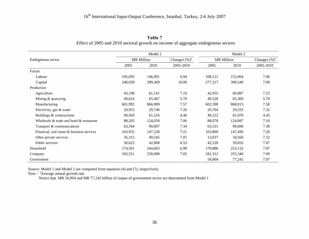
The impact of sectoral growth estimated in the Ninth Malaysia Plan on aggregate sectors is
presented in Table 7. Our results show that introducing government in the economic system
significantly improves the distribution of income. The results show that household and
labour sectors have shown among the most benefitted as a result of government
intervention. Specifically, at the end of planning period (2010), MR 152 billion of labour
income is created, larger than amount of income generated from Model 1 (MR 147 billion)
16th International Input-Output Conference, Istanbul, Turkey, 2-6 July 2007
19
and grow by 7.07 per cent. Since labour income is the primary source of household income
which is expressed in terms of compensation of employees as they received when
supplying input, thus, the large increase in labour income is expected to generate a large
benefit to household through the mechanism of labour market. As a consequence,
household income increase from MR 180 billion to MR 253 billion in 2010 higher than
those estimated from Model 1. Despite improving the distribution of income, government
intervention also on the other hand gives adverse effect to the other sectors compared to
without its intervention. For instance, the growth rate of capital income estimates from
Model 2 is lower than Model 1 by 7.06 per cent and 10 per cent, respectively. Similarly,
income of agriculture and other private services sectors generated from Model 2 is lower
than Model 1.
<Table 7>
Disaggregating household into different categories of ethnics and regions, Table 8
presents the impact of sectoral growth on household income distribution. Both models
show that the improvement in income of all ethnic groups between 2005 and 2010 is
largely explained by the increase in income of urban household. However, despite the
urban household contributes significantly to the total household incomes, our results reveal
that the growth rate estimates in the Ninth Malaysia Plan gives more opportunities to the
rural household to increase their level of income. It is observed that the growth rate of
income in the rural area is slightly higher than that in the urban area. Nevertheless, the gap
between total incomes earned by the rural and urban households is still widening. Perhaps,
the large income differential between rural and urban exist because most of the productive
industrial activities are located in the urban area and tends to hire high wage rate than rural
area which is later directly reflect the small size of multipliers for the rural household.
<Table 8>
Even though both models indicate the improvement in income for all ethnic groups,
the growth rates of income among them are differs significantly. In between 2000 and
2005, both models indicate Chinese registers the highest growth rate of income, followed
by Indian. The growth rate of the Malay’s income on the other hand relatively register

16th International Input-Output Conference, Istanbul, Turkey, 2-6 July 2007
20
among the lowest compared to Chinese and Indian for both rural and urban areas. In
contrast, the sectoral growth rates estimates in the Ninth Malaysia Plan gives more
opportunities to Malay to increase their income. The growth rate of Malay’s income
registers the second highest after Indian by 7 per cent (Model 1) and 7.11 per cent (Model
2) between 2005 and 2010. Relatively, Chinese income record among the lowest growth
rate compared to Indian and Malay. Hence, the rate of sectoral growth estimates in the
Ninth Malaysia Plan not only give more benefits to the low income group (mainly Malay),
also create opportunities to rural household to increase their level of income.
In an absolute term, our results reveal that Malay’s income register the highest
impact than other communities as a consequence of growth. However, it does not imply
that each of Malay receive the highest income among each of the rest of the ethnic groups.
It is important to note that the exercise of calculating household income through SAM
multipliers capture the effect on total income of each of the household groups, ignoring the
number households8 in the economy. Therefore, we continue our analysis by dividing the
total household income with its respective number of households in the respective groups.
This will give us the per capita or mean incomes received by each of the members of
respective ethnic groups. In fact, this analysis also can be used to answer the crucial
question of “who gets what out of national growth?” The number of household by each of
the groups is obtained directly from the HIS survey. Due to unavailability data on number
of household by employment status at ethnic and region levels, therefore, we assume that
the growth rate of household among ethnic groups and regions are constant during the
period of the study.
After obtaining mean household income, we can use those figures to calculate
household income disparity ratio among ethnic groups and use it as an inequality indicator.
Table 9 shows the household income disparity ratios for the base-year, 2005 and 2010,
derived from the both models. Compare to the base-year inequality, the results indicate that
8 Household can be distinguished according to their employment status (see Pyatt and Round, 1984). In this study, we take into account the number of household according to their employment status which comprise of employee, employer or self-employed and other (housewives, retired person, student, etc).

16th International Input-Output Conference, Istanbul, Turkey, 2-6 July 2007
21
income inequality among ethnic groups estimated from Model 1 is larger than Model 2. For
instance, income inequality estimated from Model 1 reveal that inequality between Malay
and Chinese is increased from 1:1.7419 to 1:1.9227 in 2005 while in Model 2, inequality
between these groups increased to 1:1.7665. These results imply that government
intervention in the economic system has significant impact in reducing income inequality
among household through the redistribution mechanism. Despite there is a small degree of
changes in disparity ratios9 are observed in Model 1 and Model 2 within 2005-2010, in
general, both models tend to show the same patterns of income inequality. Take inequality
between Malay and Chinese as an example, both models show that the income inequality of
these groups increase between base-year and 2005, and reduce in between 2005 and 2010
periods. Similarly, the up ward trend of inequality is observed in both models for Malay
and Indian. It can be verified that given fixed income coefficient and with the existing
market mechanism, government intervention can only reduce overall inequality but not
relatively reduce inter-ethnic inequality. Therefore, it is strongly suggests that effort to
reduce income inequality can be more effectives if equality-enhancing redistributive policy
is carefully designed to benefit the low-income group of household.
<Table 9>
The results also reveal that the sectoral growth rate estimate in the Ninth Malaysia
Plan has significant impact on reducing Malay-Chinese income inequality, but not for
Malay-Indian inequality. As indicated in Table 8, the higher rate of growth of Indian
income than Malay contributes this upward inequality trend. On the other hand, it is
observed that the major source of income inequality among ethnic groups is largely
explained by regional inequality. Specifically, the income gap among ethnic groups is
higher in rural rather than urban area. For example, Model 1 shows that each ringgit earned
by rural-Malay in 2010 is equivalent to 1.9487 ringgit earned by rural-Chinese and 1.9106
9 It was observed that there are small changes in disparity ratios within 2005-2010 for both models. For example, in Model 1, disparity ratio between Malay and Chinese improve by 0.0037 (1.9227-1.9190) while in Model 2, it improve by 0.0082 (1.7665-1.7583). Similarly, Model 1 estimates disparity ratio between Malay and Indian larger than Model 2 by 0.0061 (1.6141-1.6080) and 0.0026 (1.5371-1.5345), respectively.

16th International Input-Output Conference, Istanbul, Turkey, 2-6 July 2007
22
ringgit by rural-Indian. In contrast, the income gap between Malay-Chinese and Malay-
Indian in the urban lower than rural area by 1.4592 and 1.2209, respectively. Therefore, the
distribution of income among the various income groups in both the rural and urban areas
indicates that rural areas not only generate relatively smaller incomes for almost all ethnic
groups but also exhibit more unequal distribution of income than in urban areas.
6.2 Decomposition Impact on Household Income
Our model allows to examine in details the role of government in affecting the distribution
of income by disaggregating the impact into distributional and inter-dependency effects.
The former is further decomposed into three separate effects, namely industrial, direct and
transfer effects. The industrial effect captures the effect on output of production activities as
a result of an increase in final demand through the inter-industry relationship. As a
consequence, an additional factor input in the form of labour and capital is required to
support the additional production output. This consequence is captured by direct effect -
depending to factor endowment of the respective household groups. Transfer and
remittances from other institutions i.e. company and government is captured by transfer
effect.
Taking the difference in sectoral demands between 2005 and 2010 as an exogenous,
our decomposition results in Table 10 reveal that the impact of growth on household
income distribution is largely explained by distributional effect especially direct effect.
More than 70 per cent of household income derived from Model 1 is generated from direct
effect. In comparison, Model 2 estimates the share of direct effect decrease despite it still
contributing the largest impact on household income. It can be verified that the decreasing
share of direct effect mainly because the level of sectoral demands applied in Model 2 is
relatively low than Model 1. Low level of demand implies low sectoral output generated
and as a consequence, less amount of labour is required which then translated into income
generation. Nevertheless, this effect shows only the first round effect and does not takes
into account the full circular effects after considering other effects i.e. consumption effect
as explained by the inter-dependency effect.
16th International Input-Output Conference, Istanbul, Turkey, 2-6 July 2007
23
<Table 10>
With government interaction, it is observed that the inter-dependency effect
significantly generates large impact to household income. This implies, the diversification
of household and government consumption on commodities have greater inter-sectoral
linkages on production side which later indirectly translated into household income through
labour market. The other effects such as transfer effect does not only contribute small
portion amount of income in both approaches but also not significantly variance among
households. On the other hand, there is no industrial effect captured by household as this
effect reflects only at inter-industry level.
Looking the impact across individual household group, the results show that all the
effects derived from Model 1 reveal much smaller variances compared to Model 2. Thus, it
is strongly suggests that government interaction in the market has influenced significantly
on distribution of income especially to improve the low-income group household. As
shown in Table 10, income of Malay and Other groups improve substantially, which is
largely derived from the inter-dependency effect compared to Model 1. The share of inter-
dependency effect contributes 40 per cent and 39 per cent of total income of Malay and
Other groups, respectively, higher than Chinese and Indian. Contrary, it is observed that
direct effect generates a large impact to Chinese and Indian compared to Malay and Other.
This important result tends to explain why the only small changes in degree of inequality
are observed in Table 9. Although overall inequality reduced significantly as a result of
government intervention (Table 9), in relative the inter-ethnic inequality still does not much
improve because of rigidity of labour market. As explained by direct effect in Table 10,
Chinese and Indian generate large share of income from labour market whereas Malay and
Other register among the lowest share. In fact, the large reducing in overall inequality
estimated from Model 2 because government intervention has created large income effect
from the inter-dependency effect rather than direct effect. Thus, besides showing labour
market plays an important role in influencing distributional of income, it also observes that
there is a labour imbalance among ethnic groups in the economy. Labour imbalances can

16th International Input-Output Conference, Istanbul, Turkey, 2-6 July 2007
24
exist probably because of two reasons – skilled differential among races and wage
differential between public and private sectors.
7. Conclusions
In this paper, we examine the impact of Ninth Malaysia Plan growth on household income
distribution by employing two types of SAM models. Besides conventional approach of
Pyatt and Round (1979), we introduce an alternative approach by treating government as an
endogenous component together with production, factor, household and company. Unlike
the former approach, this approach however cannot be applied directly as supply and
demand derived is not internally consistent. To solve this issue, we modify the latter
approach by employing mixed endogenous-exogenous variables to the SAM multiplier. By
introducing government as an endogenous account in the model of multipliers, we capture
the redistribution income effect through the public expenditure and transfer when the
government receives additional revenues.
Assuming there are no changes in development policy and without policy
interventions to change the distribution of income, we find that sectoral growth estimates in
the plan period give better implication to the distributional of income. It shows that the
sectoral growth rates estimates in the Ninth Malaysia Plan gives more benefits to the low-
income group especially Malay to improve their level of income. Both models estimate the
growth rate of income of Malay is higher than high-income group i.e. Chinese. The results
also reveal inequality in income among ethnic groups is largely explained by regional
income gap. The distribution of income among the various ethnic groups indicates that rural
area not only generate smaller income for almost all ethnic groups but also exhibit more
unequal distribution of income.
The government intervention has significant impact in reducing inequality among
ethnic groups. By disaggregating the impact into distributional and inter-dependency
effects, we observe that the latter effect generates large impact to improve low-income
group especially Malay and Other. We are also find that source of inter-ethnic inequality in

16th International Input-Output Conference, Istanbul, Turkey, 2-6 July 2007
25
the economy is largely explained by unbalancing in labour structure. Our results reveal the
high-income group i.e. Chinese and Indian generate large share of income from labour
market compared to the low income group. As labour income is the primary source of
household income, therefore, from distributional planning point of views, the central focus
for overcoming ethnic income inequality should be centered on the status and earnings in
paid employment. Indeed, the effective way to reduce inequality is through formulating
policy intervention on the supply side, i.e. restructuring sectoral employment by correcting
the institutional imbalances.
References
Adelman, I., and Morris, C.T. (1973) Economic Growth and Social Equity in
Developing Countries (Standford, Standford University Press).
Adelman, I., and Robinson, S. (1978) Income Distribution Policy in Developing
Countries (Washington, Oxford University Press).
Anand, S. (1983) Inequality and Poverty in Malaysia: Measurement and
Decomposition (Washington, Oxford University Press).
Chander, R.G., Gnasegarah, S., Pyatt, G., and Round, J.I. (1980) Social Accounts and the
Distribution of Income: the Malaysian Economy in 1970, Review of Income and Wealth,
1 (26), 67-85.
Department of Statistics (2000) Report on Household Expenditure Survey 1988/89
(Kuala Lumpur, Percetakan Nasional Malaysia Berhad).
Department of Statistics (2000) Malaysia Standard Industrial Classification, 2000
(Kuala Lumpur, Percetakan Nasional Malaysia Berhad).
Department of Statistics (2001) Labour Force Survey (Kuala Lumpur, Percetakan
Nasional Malaysia Berhad).

16th International Input-Output Conference, Istanbul, Turkey, 2-6 July 2007
26
Department of Statistics (2004) Annual National Product and Expenditure Accounts
1987-2003 (Kuala Lumpur, Percetakan Nasional Malaysia Berhad).
Department of Statistics (2005) Yearbook of Statistics, 2004 (Kuala Lumpur, Percetakan
Nasional Malaysia Berhad).
Department of Statistics (2006) Input-Output Tables 2000 (Kuala Lumpur, Percetakan
Nasional Malaysia Berhad)
Economic Planning Unit. (various years) Malaysia Plan (Kuala Lumpur, Percetakan
Nasional Malaysia Berhad).
Economic Planning Unit. (2006) Ninth Malaysia Plan 2006-2010 (Kuala Lumpur,
Percetakan Nasional Berhad).
Faaland, J., Parkinson, J.R., and Saniman, R. (1990) Growth and Ethnic Inequality:
Malaysia’s New Economic Policy (Kuala Lumpur, Dewan Bahasa dan Pustaka).
Hayden, C., and Round, J.I. (1982) Developments in Social Accounting Methods as
Applied to the Analysis of Income Distribution and Employment Issues, World
Development, 10 (6), 451-465.
Khan, H.A., and Thorbecke, E. (1989) Macroeconomic Effects of Technology Choice:
Multiplier and Structural Path Analysis within a SAM Framework, Journal of Policy
Modelling, 11 (1), 131-156.
Llop, M. and Manresa, A. (2004) Income Distribution in a Regional Economy: a SAM
Model, Journal of Policy Modeling, 26 (6), 689-702.
Miller, R.E., and Blair, P.D. (1985) Input-Output Analysis: Foundations and Extensions
(Engelwood, Cliffs, Prentice-Hall).
16th International Input-Output Conference, Istanbul, Turkey, 2-6 July 2007
27
Muller, E.N. (1988a). Democracy, Economic Development, and Income Inequality,
American Sociological Review, 53 (1), 50-68.
Muller, E.N. (1988b) Inequality, Repression, and Violance: Issues of Theory and Research
Design, American Sociological Review, 53 (5), 799-806.
Nagel, J. (1974) Inequality and Discontent: a Nonlinear Hypothesis, World Politics, 26 (4),
453-472.
Lucas, R.E.B., and Verry, D.W. (1996) Growth and Income Distribution in Malaysia,
International Labour Review, 135 (5), 553-575.
Pyatt, G., and Thorbecke, E. (1976) Planning Techniques for a Better Future (Geneva,
International Labour Office).
Pyatt, G., and Round, J.I. (1979) Accounting and Fixed Price Multipliers in a Social
Accounting Matrix Framework, The Economic Journal, 89 (356), 850-873.
Pyatt, G and Round, J.I. (1984) Improving the Macroeconomic Data Base a SAM for
Malaysia, 1970, World Bank Staff Working Paper No. 646 (Washington, World Bank).
Pyatt, G. (1988) A SAM Approach to Modelling, Journal of Policy Modelling, 10 (3),
327-352.
Saari, M.Y. (2007) Development of a Social Accounting Matrix and its Application to the
Analysis of Income Distribution, In SOM PhD Conference (Groningen: SOM).
Schwartz, G., and Ter-Minassian, T. (2000) The Distributional Effects of Public
Expenditure, Journal of Economic Surveys, 14 (3), 337-358.
Shari, I. (2000) Economic Growth and Income Inequality in Malaysia, 1971-95, Journal of
the Asia Pasific Economy, 5 (1/2), 112-124.
16th International Input-Output Conference, Istanbul, Turkey, 2-6 July 2007
28
Tanzi, V. (1998) Macroeconomic Adjustment with Major Structural Reforms: Implication
for Employment and Income Distribution. In V. Tanzi and K. Chu (eds), Income
Distribution and High-Quality Growth (Cambridge, MIT Press).
Thorbecke, E., and Jung, H-S. (1996) A Multiplier Decomposition Method to Analyse
Poverty Alleviation, Journal of Development Economics, 48 (2), 297-300.
Thorbecke, E., and Charumilind, C. (2002) Economic Inequality and Its Socioeconomic
Impact, World Development, 30 (9), 1477-1495.

16th International Input-Output Conference, Istanbul, Turkey, 2-6 July 2007
29
Appendix
In the SAM frame, demand (injection) into the endogenous accounts and supply (leakage)
derived can be shown by the following accounting balance equations.
Table A: Accounting balance equations
Expenditures
Receipts Endogenous accounts Exogenous accounts Totals
Endogenous accounts N = A y (A1) X y = n + x (A3) = A y + x (A4)
Exsogenous accounts L = Ã y (A2) R ŷ = 1 + Ri (A5)= Ã y + Ri (A6)
Totals y’ = (i’A + i’Ã) y (A7) ŷ’ = i’X + i’R (A9) i’ = i’A + i’ Ã (A8) Ã y – X’i = (R-R’)i (A10) λ’y = x’i (A11)
where:A = Ny -1 = matrix of average endogenous expenditure propensitiesà = Ly -1 = matrix of average propensities to leakNi = n = vector of row sums of N = AyXi = x = vector of row sums of XLi = l = vector of row sums of L = Ãyλ’ = i’à = vector of column sums of à i.e. the vector of aggregate average propensities to leak.N = matrix of transactions among endogenous accountsX = matrix of injections from exogenous into endogenous accountsL = matrix of leakages from endogenous into exogenous accountsR = matrix of transactions among exogenous accounts.
Source : Adopted from Pyatt and Round (1979)
Consistency between supply and demand in the SAM model can be represented by equation
(A11). It implies that, in aggregate, every injection into the system must equal leakages. To
satisfy equation (A11), row and column sums of equation (A7) and (A4) must be equal to
provided equation (A8) holds and similarly for row and column sums of equation (A9) and
(A6). In our study, inconsistency exists because equation (5) does not satisfy equation
(A11) condition. This condition does not satisfy because there is inconsistency in row and
column sums between equation (A7) and (A4). Specifically, in equation (5), we treat
government as an endogenous sector together with factor, production, household and
company while at the same time, its also consider as exogenous component together with
investment and exports. As a result of this specification, a row sum of equation (A7) is
lower than column sums of equation (A4).

16th International Input-Output Conference, Istanbul, Turkey, 2-6 July 2007
30
Therefore, to address this issue, the following approach is taken. Assuming three are
only three sectors involve namely production (y1), household (y2) and government (y3), the
relationship between these sectors in matrix M* of equation (5) can be represented in the
following equation.
(1 – a11) y1 – a12 y2 – a13 y3 = x1
-a21 y1 + (1 – a22) y2 – a23 y3 = x2 (A12)-a31 y1 – a32 y2 + (1 – a33) y3 = x3
Or in matrix form,
(1 – a11) -a12 -a13 y1 X1
-a21 (1 – a22) -a23 y2 = X2 (A13)-a31 -a32 (1 – a33) y3 X3
It shows that income of y1, y2 and y3 are endogenously determined by exogenous variables
of x1, x2 and x3. Therefore, this matrix reflects a complete endogenous SAM multiplier.
To be consistent between demand and supply, we can consider output of
government sector (y3) is treated as exogenous together with other component of demands
of investment and exports. Thus, equation (A12) needs to be re-arranged. Specifically,
exogenous variables of x1, x2 and y3 are put on the right-hand side and endogenous variables
of y1, y2 and x3 on the left side equation (A2).
(1 – a11) y1 – a12 y2 + 0x3 = X1 + 0X2 + a13 Y3
-a21 y1 + (1 – a22) y2 + 0x3 = 0X1 + X2 + a23 Y3 (A14)-a31 y1 – a32 y2 – x3 = 0X1 + 0X2 – (1 – a33) Y3
where capital letters represent the exogenous variables. In matrix form, equation (A14) can be re-
expressed as
(1 – a11) -a12 0 y1 X1 + a13 Y3
-a21 (1 – a22) 0 y2 = X2 + a23 Y3 (A15)-a31 -a32 -1 x3 - (1 – a33) Y3
The solution of equation (A15) then can be expressed in the following matrix notation
y = (I – Ag)-1x = Mgx* (A16)

16th International Input-Output Conference, Istanbul, Turkey, 2-6 July 2007
31
where matrix Mg is modified from original matrix M* which contains mixed element of
endogenous-exogenous variables and x* comprises of existing and the new level of
demands generated as a result of increase in output of government (y3). Indeed, income of
y1, y2 and x3 are endogenously determined by exogenous variables of x1, x2 and y3.

16th International Input-Output Conference, Istanbul, Turkey, 2-6 July 2007
32
Table 1Mean monthly households’ income by ethnic groups and regions, 1970-2002
Mean income (MR) Annual average growth (%)Household
1970 1990 2000 2002 1970-1990 1990-2002
Mean income
Bumiputera 172 940 1,984 2,376 8.9 8.0
Chinese 394 1,631 3,456 4,279 7.4 8.4
Indian 304 1,209 2,702 3,044 7.1 8.0
Other 813 955 1,371 2,165 0.8 7.1
Rural 200 957 1,718 1,729 8.1 5.1
Urban 428 1,606 3,103 3,652 6.8 7.1
Disparity ratioa
Bumiputera : Chinese 1 : 2.29 1 : 1.74 1 : 1.74 1 : 1.80
Bumiputera : Indian 1 : 1.77 1 : 1.29 1 : 1.36 1 : 1.28
Bumiputera : Other 1 : 4.73 1 : 1.02 1 : 0.69 1 : 0.91
Rural : Urban 1 : 2.14 1 : 1.67 1 : 1.81 1 : 2.11
Source : Economic Planning Unit (various years)Note: aRatio of mean Bumiputera’s income to mean non-Bumiputeras’ income. It can be
interpreted as for instance, in year 1970, each ringgit earned by Bumiputera equivalent to 2.29 ringgit earned by Chinese and so on.
Table 2Aggregate demand by expenditure category (in current prices with 1987 prices in italics)
Expenditure2005
(MR Million)a2010
(MR Million)bAverage annual growth
rate 2005-2010 (%)
Private consumption215,876131,266
340,376182,888
9.5 6.9
Public consumption64,592 38,727
88,277 50,186
6.4 5.3
Gross fixed capital formation98,930 70,175
148,169102,512
8.4 7.9
Change in stocks-1,059 -1,708
126 104
-
Exports of good and services609,133316,959
923,484445,625
8.7 7.1
Imports of good and services492,928293,391
778,213430,018
9.6 7.9
GDP at purchasers' value494,544262,029
722,219351,297
7.9 6.0
Source : Economic Planning Unit (2006)Note : Superscript (a) and (b) represent estimate and target, respectively.
16th International Input-Output Conference, Istanbul, Turkey, 2-6 July 2007
33
Table 3 (a)Sectoral final demands estimate for year 2005 (in current price)
Final Demands (MR Million)Sector Private
consumptionGovernment consumption
Change in stocks
Gross fixed capital formation
Exports Total
Agriculture 11,728 -3 1,256 6,005 18,986Mining & quarrying -146 31,599 31,453Manufacturing 59,532 5,396 396,838 461,766Construction 566 39,760 4,827 45,153Government services 24,707 2 24,708Electricity, gas & water 5,181 7 5,188Transport, storage & communications 19,192 -1 161 25,960 45,311Wholesale and hotel & restaurant 23,903 -6 2,343 12,948 39,188Financial, real estate & business services 36,722 21,805 58,528Other private services 16,381 22,596 -3 2,375 41,350Total 173,205 47,303 -160 48,915 502,367 771,630
Table 3 (b) Sectoral final demands estimates for year 2010 (in current price)
Final Demands (MR Million)Sector Private
consumptionGovernment consumption
Change in stocks
Gross fixed capital formation
Exports Total
Agriculture, forestry, livestock & fishery 16,400 1 1,806 8,123 26,330Mining & quarrying 60 39,638 39,699Manufacturing 98,911 9,393 575,213 683,517Construction 781 49,010 5,656 55,447Government services 33,722 2 33,724Electricity, gas & water 7,563 11 7,574Transport, storage & communications 31,342 1 280 37,580 69,204Wholesale and hotel & restaurant 36,597 3 3,411 17,338 57,348Financial, real estate & business services 59,909 31,856 91,765Other private services 27,275 31,500 1 3,538 62,314Total 278,777 65,221 66 63,901 718,956 1,126,921
Source: Economic Planning Unit (unpublished)

16th International Input-Output Conference, Istanbul, Turkey, 2-6 July 2007
34
Schematic SAM 2000Expenditure
1 2 3 4 5 6 7 8 9
Institutions
Current accountsRest of the World AccountsFactors of
production Production activities
Household Company Government
Capital Account
Current Capital
Indirect tax Total
1 Factor of productionValue added payment to
factors
Net factorial income
received from abroad
Total factor income
2 Production activities
Raw materials purchases of
domestic goods
Households consumption on domestic
goods
Government consumption on domestic
goods
Investment expenditure on
domestic goods
ExportsGross output (aggregate demand)
3 Household
Compensation of employee
and unincorporated business profit
Distributed profit
current transfer to household
Non-factor income from
abroad
Total household
income
4 CompanyBusiness
corporate profitcurrent transfer to companies
Non-factor income from
abroad
Total company incomes
5
Cur
rent
acc
ount
s
Government Income tax Corporate taxNon-factor
income from abroad
Indirect taxesTotal
government revenue
6 Capital accountHousehold
savingsCompanies
savingGovernment
savingsAggregate
saving
7 CurrentNet factorial income paid
abroad
Import of raw materials
Household consumption on imported
goods
Non-factor income paid
abroad
Government consumption
imports
Imports of capital goods
Balance of payment of
current account
Total imports
8 Res
t of
the
wor
ld
acco
unts
CapitalNet investment
abroad Total capital paid abroad
Inco
me
9 Indirect taxCommodity
taxesSales taxes
Taxes on imported
capital goodsExports levy
Total indirect tax
Total factor payments
Gross input (total costs)
Total household
expenditure
Total companyexpenditure
Total government expenditure
Aggregate investment
Total exportsTotal capital
received from abroad
Total indirect tax
Table 4

16th International Input-Output Conference, Istanbul, Turkey, 2-6 July 2007
35
Table 5 Disaggregation of household and labour in the SAM
Household/labour Region Ethnic Education
Household Malay Chinese Indian Other
Non-citizen
Labour Malay
Chinese Indian Other
Non-citizen
Table 6 Schematic representation of endogenous and exogenous accounts in the SAM
(1) (2) (3) (4) (5)
Factor of production (1) 0 T12 0 x1 y1
Production activities (2) 0 T22 T23 x2 y2
Institutions i.e.household and company (3) T31 0 T33 x3 y3
Sum of other accounts (4) I’1 I’2 I’3 t yx
Totals (5) y1 y2 y3 yx
Note : Italic letters refer to the endogenous accounts.
RuralUrban
RuralUrban
None educationSecondary educationTertiary education
Citizen
Citizen
Endogenous accounts
16th International Input-Output Conference, Istanbul, Turkey, 2-6 July 2007
36
Table 7 Effect of 2005 and 2010 sectoral growth on income of aggregate endogenous sectors
Model 1 Model 2
MR Million Changes (%)a MR Million Changes (%)aEndogenous sector
2005 2010 2005-2010 2005 2010 2005-2010
Factor
Labour 105,095 146,991 6.94 108,121 152,064 7.06
Capital 248,028 399,369 10.00 277,317 390,549 7.09
Production
Agriculture 43,198 61,141 7.19 42,955 60,887 7.23
Mining & quarrying 49,616 65,467 5.70 49,528 65,360 5.70
Manufacturing 601,992 866,909 7.57 602,398 868,013 7.58
Electricity, gas & water 20,953 29,746 7.26 20,764 29,555 7.32
Buildings & constructions 49,450 61,516 4.46 49,122 61,076 4.45
Wholesale & trade and hotel & restaurant 88,205 124,059 7.06 88,078 124,087 7.10
Transport & communications 63,164 90,007 7.34 63,531 90,690 7.38
Financial, real estate & business services 103,932 147,228 7.21 103,869 147,490 7.26
Other private services 35,315 49,545 7.01 13,037 18,560 7.32
Public services 30,625 42,008 6.53 42,528 59,832 7.07
Household 174,501 244,603 6.99 179,886 253,132 7.07
Company 183,551 258,089 7.05 181,312 255,340 7.09
Government 54,904 77,242 7.07
Source: Model 1 and Model 2 are computed from equation (4) and (7), respectively.Note : aAverage annual growth rate Notice that MR 54,904 and MR 77,242 billion of output of government sector are determined from Model 1

16th International Input-Output Conference, Istanbul, Turkey, 2-6 July 2007
37
Table 8 Effect of 2005 and 2010 sectoral growth on household income distribution
Model 1 Model 2
MR Million Changes (%)a MR Million Changes (%)aHouseholdBase year
(2000) 2005 2010 2000-2005 2005-2010 2005 2010 2000-2005 2005-2010
Malayb 65,910 70,122 98,347 1.25 7.00 75,466 106,399 2.74 7.11
Chineseb 57,521 67,546 94,556 3.27 6.96 66,789 93,731 3.03 7.01
Indianb 14,319 16,168 22,762 2.46 7.08 16,605 23,450 3.01 7.15
Otherb 8,446 9,447 13,216 2.26 6.95 9,652 13,569 2.71 7.05
Rural household 44,018 48,660 68,256 2.03 7.00 50,561 71,213 2.81 7.09
Rural - Malay 25,396 27,205 38,170 1.39 7.01 29,071 40,989 2.74 7.11
Rural - Chinese 10,161 11,992 16,786 3.37 6.96 11,769 16,511 2.98 7.01
Rural - Indian 3,907 4,424 6,242 2.52 7.13 4,526 6,401 2.99 7.18
Rural - Others 4,554 5,039 7,058 2.04 6.97 5,195 7,312 2.67 7.08
Urban household 102,178 114,623 160,625 2.33 6.98 117,951 165,936 2.91 7.07
Urban - Malay 40,514 42,917 60,177 1.16 6.99 46,395 65,410 2.75 7.11
Urban - Chinese 47,360 55,555 77,770 3.24 6.96 55,020 77,219 3.04 7.01
Urban - Indian 10,412 11,743 16,520 2.44 7.06 12,078 17,048 3.01 7.14
Urban - Others 3,892 4,408 6,158 2.52 6.92 4,458 6,258 2.75 7.02
Non-citizen 9,844 11,218 15,723 2.65 6.99 11,374 15,983 2.93 7.04
Source: Model 1 and Model 2 are computed from equation (4) and (7), respectively.Note : aAverage annual growth rate bThe total household income for Malay, Chinese, Indian and Other groups are obtained by adding the rural and urban incomes for the respective groups.

16th International Input-Output Conference, Istanbul, Turkey, 2-6 July 2007
38
Table 9 Household income disparity ratio as a consequence of 2005 and 2010 sectoral growth
Model 1 Model 2Household Base year
2005 2010 2005 2010
Malay : Chinese 1 : 1.7419 1 : 1.9227 1 : 1.9190 1 : 1.7665 1 : 1.7583
Malay : Indian 1 : 1.5151 1 : 1.6080 1 : 1.6141 1 : 1.5345 1 : 1.5371
Malay : Other 1 : 0.6274 1 : 0.6596 1 : 0.6579 1 : 0.6262 1 : 0.6244
Rural
Rural - Malay : Rural - Chinese 1 : 1.7730 1 : 1.9533 1 : 1.9487 1 : 1.7939 1 : 1.7851
Rural - Malay : Rural - Indian 1 : 1.7974 1 : 1.8999 1 : 1.9106 1 : 1.8190 1 : 1.8246
Rural - Malay : Rural - Others 1 : 0.7061 1 : 0.7293 1 : 0.7281 1 : 0.7036 1 : 0.7024
Urban
Urban - Malay : Urban - Chinese 1 : 1.3199 1 : 1.4616 1 : 1.4592 1 : 1.3390 1 : 1.3330
Urban - Malay : Urban - Indian 1 : 1.1467 1 : 1.2209 1 : 1.2249 1 : 1.1616 1 : 1.1629
Urban - Malay : Urban - Others 1 : 0.7126 1 : 0.7619 1 : 0.7591 1 : 0.7127 1 : 0.7097
Rural : Urban 1 : 2.2613 1 : 2.2947 1 : 2.2925 1 : 2.2726 1 : 2.2699
Source: Derived from Table 8 after diving the total income with the number of households of its respective ethnic groups.
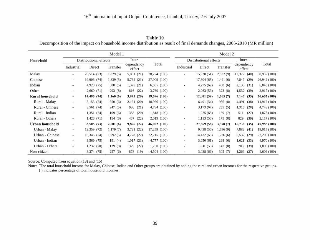
16th International Input-Output Conference, Istanbul, Turkey, 2-6 July 2007
39
Table 10 Decomposition of the impact on household income distribution as result of final demands changes, 2005-2010 (MR million)
Model 1 Model 2
Distributional effects Distributional effectsHousehold
Industrial Direct Transfer
Inter-dependency
effectTotal
Industrial Direct Transfer
Inter-dependency
effectTotal
Malay - 20,514 (73) 1,829 (6) 5,881 (21) 28,224 (100) - 15,928 (51) 2,632 (9) 12,372 (40) 30,932 (100)
Chinese - 19,906 (74) 1,339 (5) 5,764 (21) 27,009 (100) - 17,604 (65) 1,491 (6) 7,847 (29) 26,942 (100)
Indian - 4,920 (75) 300 (5) 1,375 (21) 6,595 (100) - 4,275 (62) 438 (6) 2,133 (31) 6,845 (100)
Other - 2,660 (71) 293 (8) 816 (22) 3,769 (100) - 2,063 (53) 323 (8) 1,532 (39) 3,917 (100)
Rural household - 14,495 (74) 1,160 (6) 3,941 (20) 19,596 (100) - 12,001 (58) 1,505 (7) 7,146 (35) 20,652 (100)
Rural - Malay - 8,155 (74) 650 (6) 2,161 (20) 10,966 (100) - 6,491 (54) 936 (8) 4,491 (38) 11,917 (100)
Rural - Chinese - 3,561 (74) 247 (5) 986 (21) 4,794 (100) - 3,173 (67) 255 (5) 1,315 (28) 4,743 (100)
Rural - Indian - 1,351 (74) 109 (6) 358 (20) 1,818 (100) - 1,225 (65) 139 (7) 511 (27) 1,875 (100)
Rural - Others - 1,428 (71) 154 (8) 437 (22) 2,019 (100) - 1,113 (53) 175 (8) 829 (39) 2,117 (100)
Urban household - 33,505 (73) 2,601 (6) 9,896 (22) 46,002 (100) - 27,869 (58) 3,378 (7) 16,738 (35) 47,985 (100)
Urban - Malay - 12,359 (72) 1,179 (7) 3,721 (22) 17,259 (100) - 9,438 (50) 1,696 (9) 7,882 (41) 19,015 (100)
Urban - Chinese - 16,345 (74) 1,092 (5) 4,778 (22) 22,215 (100) - 14,432 (65) 1,236 (6) 6,532 (29) 22,200 (100)
Urban - Indian - 3,569 (75) 191 (4) 1,017 (21) 4,777 (100) - 3,050 (61) 298 (6) 1,621 (33) 4,970 (100)
Urban - Others - 1,232 (70) 139 (8) 379 (22) 1,750 (100) - 950 (53) 147 (8) 703 (39) 1,800 (100)
Non-citizen - 3,374 (75) 257 (6) 873 (19) 4,504 (100) - 3,038 (66) 305 (7) 1,266 (27) 4,609 (100)
Source: Computed from equation (13) and (15) Note: aThe total household income for Malay, Chinese, Indian and Other groups are obtained by adding the rural and urban incomes for the respective groups. ( ) indicates percentage of total household incomes.

16th International Input-Output Conference, Istanbul, Turkey, 2-6 July 2007
40