the identi–cation zoo - meanings of identi–cation in ... · continued next slide ... formal...

The Identification Zoo - Meanings of Identification inEconometrics: PART 1

Arthur Lewbel

Boston College

original 2015, heavily revised 2018

Lewbel (Boston College) Identification Zoo 2018 1 / 91

The Identification Zoo - Part 1 - sections 1, 2, and 3.

(These are notes to accompany the survey article of the same name in theJournal of Economic Literature).

Well over two dozen types of identification appear in the econometricsliterature, including (in alphabetical order):

Bayesian identification, causal identification, essential identification,eventual identification, exact identification, first order identification,frequentist identification, generic identification, global identification,identification arrangement, identification at infinity, identification byconstruction, identification of bounds, ill-posed identification, irregularidentification, local identification, nearly-weak identification,nonparametric identification, non-robust identification, nonstandard weakidentification, overidentification, parametric identification, partialidentification, point identification, sampling identification, semiparametricidentification, semi-strong identification, set identification, strongidentification, structural identification, thin-set identification,underidentification, and weak identification.


1. Introduction

Econometric identification really means just one thing:

Model parameters or features uniquely determined from the observablepopulation that data are drawn from.

Goals:

1. Provide a new general framework for characterizing identificationconcepts

2. Define and summarize, with examples, the many different termsassociated with identification.

3. Show how these terms relate to each other.

4. Discuss concepts closely related to identification, e.g., observationalequivalence, normalizations, and the differences in identification betweenstructural models and randomization based reduced form (causal) models.


Table of Contents:

1. Introduction

2. Historical Roots of Identification

3. Point Identification3.1 Introduction to Point Identification3.2 Defining Point Identification3.3 Examples and Classes of Point Identification3.4 Proving Point Identification3.5 Common Reasons for Failure of Point Identification3.6 Control Variables3.7 Identification by Functional Form3.8 Over, Under, and Exact Identification, Rank and Order conditions.

4. Coherence, Completeness and Reduced Forms

Continued next slide


Table of Contents - continued:

5. Causal Reduced Form vs Structural Model Identification5.1 Causal or Structural Modeling? Do Both5.2 Causal vs Structural Identification: An Example5.3 Causal vs Structural Simultaneous Systems5.4 Causal vs Structural Conclusions

6. Identification of Functions and Sets6.1 Nonparametric and Semiparametric Identification6.2 Set Identification6.3 Normalizations in Identification6.4 Examples: Some Special Regressor Models

Continued next slide


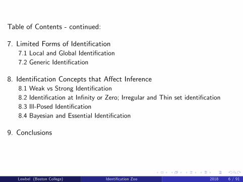
Table of Contents - continued:

7. Limited Forms of Identification7.1 Local and Global Identification7.2 Generic Identification

8. Identification Concepts that Affect Inference8.1 Weak vs Strong Identification8.2 Identification at Infinity or Zero; Irregular and Thin set identification8.3 Ill-Posed Identification8.4 Bayesian and Essential Identification

9. Conclusions


Part 2 will have sections:


5. Causal Reduced Form vs Structural Model Identification


6. Identification of Functions and Sets

7. Limited Forms of Identification

8. Identification Concepts that Affect Inference

9. Conclusions


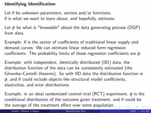
Identifying Identification

Let θ be unknown parameters, vectors and/or functions.θ is what we want to learn about, and hopefully, estimate.

Let φ be what is "knowable" about the data generating process (DGP)from data.

Example: θ is the vector of coeffi cients of traditional linear supply anddemand curves. We can estimate linear reduced form regressioncoeffi cients. The probability limits of those regression coeffi cients are φ.

Example: with independent, identically distributed (IID) data, thedistribution function of the data can be consistently estimated (theGlivenko—Cantelli theorem). So with IID data the distribution function isφ, and θ could include objects like structural model coeffi cients,elasticities, and error distributions.

Example: in an ideal randomized control trial (RCT) experiment, φ is theconditional distribution of the outcome given treatment, and θ could bethe average of the treatment effect over some population.


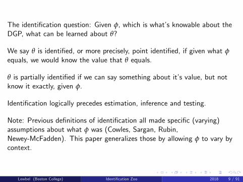
The identification question: Given φ, which is what’s knowable about theDGP, what can be learned about θ?

We say θ is identified, or more precisely, point identified, if given what φequals, we would know the value that θ equals.

θ is partially identified if we can say something about it’s value, but notknow it exactly, given φ.

Identification logically precedes estimation, inference and testing.

Note: Previous definitions of identification all made specific (varying)assumptions about what φ was (Cowles, Sargan, Rubin,Newey-McFadden). This paper generalizes those by allowing φ to vary bycontext.


2. The Historical Roots of Identification

Before identification we need the notion of "ceteris paribus," that is,holding other things equal.

Formal application of this concept to economics attributed to AlfredMarshall (1890).

But earliest economic example is from William Petty (1662), "A Treatiseof Taxes and Contributions:"

"If a man can bring to London an ounce of Silver out of the Earth in Peru,in the same time that he can produce a bushel of Corn, then one is thenatural price of the other; now if by reason of new and more easie Mines aman can get two ounces of Silver as easily as formerly he did one, thenCorn will be as cheap at ten shillings the bushel, as it was before at fiveshillings caeteris paribus."

This may be the earliest example of identification: a claimed causal effecton prices.


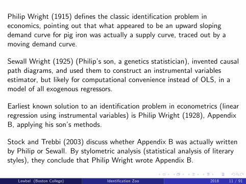
Philip Wright (1915) defines the classic identification problem ineconomics, pointing out that what appeared to be an upward slopingdemand curve for pig iron was actually a supply curve, traced out by amoving demand curve.

Sewall Wright (1925) (Philip’s son, a genetics statistician), invented causalpath diagrams, and used them to construct an instrumental variablesestimator, but likely for computational convenience instead of OLS, in amodel of all exogenous regressors.

Earliest known solution to an identification problem in econometrics (linearregression using instrumental variables) is Philip Wright (1928), AppendixB, applying his son’s methods.

Stock and Trebbi (2003) discuss whether Appendix B was actually writtenby Philip or Sewall. By stylometric analysis (statistical analysis of literarystyles), they conclude that Philip Wright wrote Appendix B.


Aside: Sewall Wright’s first application of causal path diagrams was todetermine the extent to which fur color in guinea pigs was determined bydevelopmental vs genetic factors. See, e.g., Pearl (2018).

So while the father looked at pig iron, the son studied actual pigs.

In addition to two different Wrights, two different Workings also worked onthe subject

Holbrook Working (1925) and, more relevantly, Elmer J. Working (1927).Both wrote about statistical demand curves (Holbrook is the one forwhom the Working-Leser Engel curve is named).

Jan Tinbergen (1930) proposed indirect least squares estimation, but likeSewall Wright, only for convenience not for solving identification.


Others on identification with simultaneity: Trygve Haavelmo (1943),Tjalling Koopmans (1949), Theodore W. Anderson and Herman Rubin(1949), Koopmans and Olav Reiersøl (1950), Leonid Hurwicz (1950),Koopmans, Rubin, and Roy B. Leipnik (1950), and the work of the CowlesFoundation.

Related important early work: Abraham Wald (1950), Henri Theil (1953),J. Denis Sargan (1958), Franklin Fisher (1966), and (using errorrestrictions) Karl G. Jöreskog (1970).

Milton Friedman (1953) critiques Cowles foundation work - warns againstusing different criteria to select models versus criteria to identify them.


A different problem: Causal Modeling - Identifying a treatment effect.

Identification based on randomization: Jerzy Neyman (1923), David R.Cox (1958), Donald B. Rubin (1978), many others.

In contrast to random selection, econometricians historically focused oncases where selection (who is treated or observed) and outcomes arecorrelated. Sources of correlation:

Simultaneity as in Trygve Haavelmo (1943). Pearl (2015) and Heckmanand Pinto (2015) credit Haavelmo as the first rigorous treatment ofcausality in the context of structural econometric models.

Optimizing self selection as in Andrew D. Roy (1951).Survivorship bias as in Abraham Wald (1943) - treatment assignment israndom, but sample attrition is correlated with outcomes (WW II planeshit randomly, only ones hit in survivable spots return to be observed).General models where selection and outcomes are correlated - James J.Heckman (1978).Formal use of Causal Diagrams: Pearl (1988)


Another identification problem: identifying true linear regressioncoeffi cients when regressors are measured with error.

Robert J. Adcock (1877, 1878), and Charles H. Kummell (1879):measurement errors in "Deming regression", (popularized in stats lit by W.Edwards Deming 1943). Is regression that mins least squares errorsmeasured perpendicular to the fitted line.

Corrado Gini (1921) gave an estimator for measurement errors in standardlinear regression.Ragnar A. K. Frisch (1934) was first to discuss the issue in a way thatwould now be recognized as identification.

Other early papers looking at measurement errors in regression includeNeyman (1937), Wald (1940), Koopmans (1937), Reiersøl (1945, 1950),Roy C. Geary (1948), and James Durbin (1954).

Tamer (2010) credits Frisch (1934) as also being the first in the literatureto describe an example of partial or set identification.


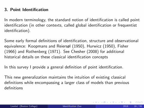
3. Point Identification

In modern terminology, the standard notion of identification is called pointidentification (in other contexts, called global identification or frequentistidentification).

Some early formal definitions of identification, structure and observationalequivalence: Koopmans and Reiersøl (1950), Hurwicz (1950), Fisher(1966) and Rothenberg (1971). See Chesher (2008) for additionalhistorical details on these classical identification concepts

In this survey I provide a general definition of point identification.

This new generalization maintains the intuition of existing classicaldefinitions while encompassing a larger class of models than previousdefinitions


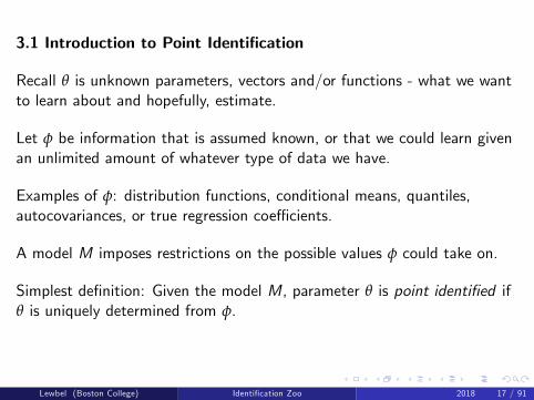
3.1 Introduction to Point Identification

Recall θ is unknown parameters, vectors and/or functions - what we wantto learn about and hopefully, estimate.

Let φ be information that is assumed known, or that we could learn givenan unlimited amount of whatever type of data we have.

Examples of φ: distribution functions, conditional means, quantiles,autocovariances, or true regression coeffi cients.

A model M imposes restrictions on the possible values φ could take on.

Simplest definition: Given the model M, parameter θ is point identified ifθ is uniquely determined from φ.


Usually think of a model M as set of equations describing behavior.

More generally, a model corresponds to assumptions about and restrictionson the DGP.

This includes assumptions about the behavior that generates the data, andabout how the data are collected and measured.

These assumptions in turn imply restrictions on φ and θ.

So, identification (even in purely experimental settings) always entails amodel.


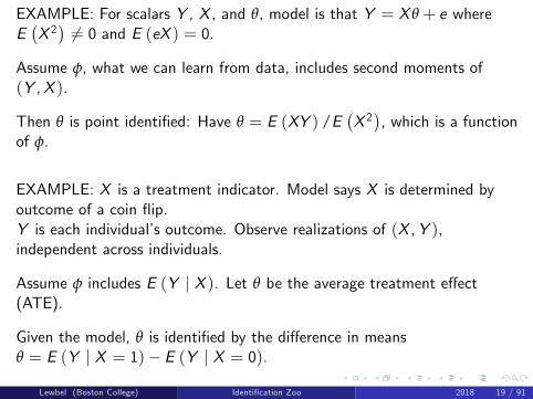
EXAMPLE: For scalars Y , X , and θ, model is that Y = X θ + e whereE(X 2)6= 0 and E (eX ) = 0.

Assume φ, what we can learn from data, includes second moments of(Y ,X ).

Then θ is point identified: Have θ = E (XY ) /E(X 2), which is a function

of φ.

EXAMPLE: X is a treatment indicator. Model says X is determined byoutcome of a coin flip.Y is each individual’s outcome. Observe realizations of (X ,Y ),independent across individuals.

Assume φ includes E (Y | X ). Let θ be the average treatment effect(ATE).

Given the model, θ is identified by the difference in meansθ = E (Y | X = 1)− E (Y | X = 0).


Both of the examples assume expectations of observed variables areknowable, and so can be included in φ.

To justify the assumption, might appeal to statistical properties of(observable) sample averages:

Unbiasedness or (given a weak law of large numbers) consistency.

The definition of identification is somewhat circular:

Start by assuming something, φ, is identified to end by determining ifsomething else, θ, is identified.

Assuming φ is knowable, or identified, must be justified by deeperassumptions regarding the underlying DGP (Data Generating Process).


Common DGP assumptions:

1. IID (Independently, Identically Distributed) observations of a vector W ,with sample size n→ ∞.With such data can consistently estimate the distribution of W by theGlivenko—Cantelli theorem.So reasonable to assume knowable φ is the distribution function of W .

2. Each observation of X is a value chosen by experiment.Conditional on that value of X , randomly draw an observation of Y ,(independent of other observations).φ is the conditional distribution function of Y given X .φ is only knowable for values of X that can be set by the experiment.

3. Stationary time series data: φ is variances and autocovariancesNot higher moments if they could be unstable over time.


φ depends on the model.

Example: In dynamic panel data models, the Arellano and Bond (1991)estimator is based on moments that are assumed knowable (can beestimated from data) and equal zero in the population.

Blundell and Bond (1998) provides additional moments (functional forminformation about the initial time period zero). Possible that θ is notidentified with Arellano and Bond moments, but becomes identified if themodel restricts φ by assuming Blundell and Bond moments also hold.

Example: experimental design, random assignment into treatment andcontrol groups. Still need a model for identification of treatment effects.Typical model assumptions rule out measurement errors, sample attrition,censoring, social interactions, and general equilibrium effects.


Two types of DGP assumptions.

1. Assumptions regarding collection of data, e.g., selection, measurementerrors, and survey attrition.

2. Assumptions regarding generation of data, e.g., randomization orstatistical and behavioral assumptions.

Arellano (2003) refers to a set of behavioral assumptions that suffi ce foridentification as an identification arrangement.

Both types of assumptions determine the model M and what is knowableφ, and hence determine what identification is possible.


Identification logically precedes estimation. If θ is not point identified,then estimators for θ having some desirable properties (like consistency)will not exist.

However, identification does not by itself imply that estimators with anyparticular desired properties exist, only that they might.

Example: Suppose θ = E (X ), and the DGP is such that θ is finite. Withiid observations of X , we can show that θ = E (X ) is identified.

We might desire an estimator for θ = E (X ) that converges in meansquare, but if X has suffi ciently thick tails, then no such estimator mayexist.

Ill-conditioned identification and non-robust identification (discussed laterin Section 8) are two situations where, despite being point identified, anyestimator of θ will have some undesirable properties.


Big Data

In some ways, ’big data’is (or should be) about identification.

Varian (2014) says, "In this period of “big data,” it seems strange to focuson sampling uncertainty, which tends to be small with large datasets, whilecompletely ignoring model uncertainty, which may be quite large."

In big data, the observed sample is so large that it can treated as if it werethe population.

Identification deals precisely with what can be learned about therelationships among variables given the population.


3.2 Defining Point Identification

Recall φ is a set of constants and/or functions that we assume are known,or knowable, given the DGP.

Examples: φ could be:i. the distribution of Y ,X if IID observations.ii. means and autocovariances in stationary dataiii. reduced form linear regression coeffi cientsiv. conditional distribution of Y given X where X values are set byexperiment.v. transition probabilities, if W follows a martingale process.

Previous definitions of point identification in the literature each startedfrom a particular definition of φ. Examples:— in Matzkin (2007, 2012), φ is a distribution function.— In textbook linear supply and demand curves, φ is regressioncoeffi cients.

This survey generalizes and encompasses previous definitions by allowing φto depend on context.


Recall parameters θ are a set of unknown constants and/or functions thatcharacterize or summarize relevant features of a model.

θ can be anything we might want to estimate (θ will generally beestimands, i.e., population values of estimators of objects that we want tolearn about).

Examples θ could include regression coeffi cients, the sign of an elasticity,an average treatment effect, or an error distribution.

θ may also include "nuisance" parameters, which are defined asparameters that are not of direct economic interest, but may be requiredfor identification and estimation of other objects that are of interest.


Rough definitions of observational equivalence and of pointidentification:

Two possible values θ and θ are observationally equivalent if there exists avalue of φ that could imply either θ and θ.

θ is point identified if θ and θ being observationally equivalent implies θand θ are equal.

That is, θ is point identified if each possible value of φ implies a uniquevalue of θ.

The remainder of this subsection (which can be skipped if one’s primaryinterest is in later sections) defines point identification a little moreprecisely.

A more mathematically rigorous definition is provided in the Appendix ofthe Identification Zoo survey.


Definitions:

A model M is a set of functions or sets that satisfy some givenrestrictions.

M can include restrictions on regression functions, distribution functions oferrors or other unobservables, utility functions, payoff matrices, orinformation sets.

A model value m ∈ M is an element of M. So m is a particular value ofthe functions, matrices, and sets that comprise the model.

Example: If Yi = g (Xi ) + ei , then M could be the set of possibleregression functions g and the set of possible joint distributions of theregressor Xi and the error term ei for all i in the population.

The elements of M could be restricted: e.g., require linearityg (Xi ) = a+ bXi . Other possible restrictions: var (ei ) finite,E (ei | X ) = 0.


Each model value m ∈ M generally implies a unique data generatingprocess (DGP). Exceptions are incoherent models - see section 4.

Assume each model value m ∈ M implies a particular value of φ and of θ.

Violations of this assumption can lead to incoherence or incompleteness -see section 4.

There could be many values of m that imply the same φ or the same θ.

Define the structure s (φ, θ) to be the set of all m that yield both thegiven values of φ and of θ.

Let Θ denote the set of all possible values that the model says θ could be.


Two parameter values θ and θ are defined to be observationally equivalentif there exists a φ such that both s (φ, θ) and s

(φ, θ)are not empty.

θ and θ observationally equivalent means there exists a φ and modelvalues m and m such that m implies the values φ and θ, and m implies thevalues φ and θ..

Definition of Identification:

The parameter θ is defined to be point identified (often just calledidentified) if there do not exist any pairs of possible values θ and θ in Θthat are different but observationally equivalent.


Let θ0 be the unknown true value of θ.

The particular value θ0 is point identified if θ0 not observationallyequivalent to any other θ in Θ.

But we don’t know which of the possible values of θ ∈ Θ is θ0.

So to ensure point identification, we generally require that no twoelements θ and θ in the set Θ having θ 6= θ be observationally equivalent.

Sometimes this condition is called global identification rather than pointidentification, to explicitly say that θ0 is point identified no matter whatvalue in Θ turns out to be θ0.


Showing identification in theory

We have defined point identification of parameters θ.

We say that the model is point identified when no pairs of model values mand m in M are observationally equivalent (treating m and m as if theywere the parameters θ).

Identification of the model implies identification of any model parametersθ.

We define the model M, so we could in theory1. enumerate every m ∈ M,2. list every φ and θ that is implied by each m, and thereby determineevery s (φ, θ)

3. check every value of every pair of structures s (φ, θ) and s(

φ, θ)to see

if θ is point identified or not.

The diffi culty of proving identification in practice is in finding tractableways to accomplish this enumeration.


Misspecification

Let φ0 be the value of φ that corresponds to the true DGP.

A model M is defined to be misspecified if there does not exist any modelvalue m ∈ M that yields φ0.

Misspecification means that what we can observe about the true DGP,which is φ0, cannot satisfy the restrictions of the model M.

If our model M is not misspecified, then there exists a model value m0which implies φ0.

What is the true model value? What is meant by truth of a model, sincemodels only approximate the real world?

We avoid that question, by just saying that, whatever the "true" modelvalue m0 is, it has the property of not conflicting with what we canpotentially observe or know, which is the true φ0.


Additional Definitions

Ensuring point identification can require ruling out some potential valuesof θ.

Local and generic identification are examples (are discussed in more detaillater)

Local identification of θ means that there exists a neighborhood of θ suchthat, for all values θ in this neighborhood (other than the value θ) θ is notobservationally equivalent to θ.

Generic identification means that set of values of θ in Θ that cannot bepoint identified is a very small subset (formally, a measure zero subset) ofΘ.


θ0 is said to be set identified (or partially identified) if there exist somevalues of θ ∈ Θ that are not observationally equivalent to θ0.

The only time a parameter θ is not set identified is when all θ ∈ Θ areobservationally equivalent.

The identified set is the set of all values of θ ∈ Θ that are observationallyequivalent to θ0.

Point identification of θ0 is when the identified set contains only oneelement, which is θ0.


Parametric identification is where θ is a finite set of constants, and allvalues of φ correspond to values of a finite set of constants.

Nonparametric identification is where θ consists of functions or infinitesets.

Other cases are called semiparametric identification, e.g., θ includes both avector of constants and some functions.


3.3 Examples and Classes of Point Identification

Example 1: a median.M is set of possible distributions of continuous W with strictlymonotonically increasing distribution functions F (w).DGP is IID draws of W . Each φ is an F function.Each model value m happens to correspond to a unique value of φ.

Let θ be the median of W .The structure s (F , θ) has one element if F (θ) = 1/2, is empty otherwise.No pair θ 6= θ are observationally equivalent, because F (θ) = 1/2 andF(

θ)= 1/2 implies θ = θ.

θ is identified because it’s the unique solution to F (θ) = 1/2. KnowingF , we can determine θ.


Example 2: Linear regression.DGP is observations of Y ,X where Y is a scalar, X is a K−vector.Observations of Y , X might not be IID.φ is first and second moments of X and Y . Assumed finite, constantacross observations.M is the set of joint distributions of e,X that satisfy Y = X ′θ + e,E (Xe) = 0 for an error term e.s (φ, θ) is nonempty when moments comprising φ satisfyE [X (Y − X ′θ)] = 0 for the given θ.

If restrict M by assuming E (XX ′) is nonsingular, then θ identified byθ = E (XX ′)−1 E (XY ).Otherwise θ = E (XX ′)− E (XY ) for different pseudoinverses E (XX ′)−

are observationally equivalent.

Identification is parametric: θ and φ are finite vectors.Would be semiparametric if, e.g., assumed φ was distribution of Y ,Xunder IID data, and parameter set included the distribution function of e.


Example 3: treatment.

DGP: Assign treatment T = 0 or T = 1, generate an outcome Y .Y ,T independent across individuals. φ is distribution of Y ,T .

Rubin (1974) causal notation: Random Y (t) is the outcome an individualwould have if assigned T = t.θ is the average treatment effect (ATE), defined byθ = E (Y (1)− Y (0)).M is the set of all possible joint distributions of Y (1), Y (0), and T .A restriction on M: Rosenbaum and Rubin’s (1983) assumption that(Y (1) ,Y (0)) is independent of T .Rubin (1990) calls this unconfoundedness, is equivalent to randomassignment of treatment.

θ is identified because unconfoundedness implies thatθ = E (Y | T = 1)− E (Y | T = 0).


Heckman, Ichimura, and Todd (1998): a weaker suffi cient condition foridentification of θ is the mean unconfoundedness assumption thatE (Y (t) | T ) = E (Y (t)).

Without some form of unconfoundedness, θ might not equalE (Y | T = 1)− E (Y | T = 0).

More relevantly for identification, without unconfoundedness, differentjoint distributions of Y (1), Y (0), and T (i.e., different model values m)might yield the same joint distribution φ, but have different values for θ.

Those different θ values would then be observationally equivalent to eachother, and so we would not have point identification.

Above can all be generalized to allow for covariates. The key foridentification is not a closed form expression likeE (Y | T = 1)− E (Y | T = 0) for θ. The key is a unique value of θ foreach possible φ.


Example 4: linear supply and demand.

In each time period, demand Y = bX + cZ + U and supply Y = aX + ε.Y quantity, X price, Z income, U, ε mean zero errors, independent of Z .Each model value m consists of a particular joint distribution of Z , U, andε in every time period.These distributions could change over time.

φ could be vector (φ1, φ2) of reduced form coeffi cients Y = φ1Z + V1and X = φ2Z + V2 where V1 and V2 are mean zero, independent of Z .Solving for the reduced form coeffi cients: φ1 = ac/ (a− b) andφ2 = c/ (a− b).


Demand Y = bX + cZ + U and Supply Y = aX + ε.Let θ be a, the supply price coeffi cient.

A given structure s (φ, θ) contains all model values m that satisfy θ = a,φ1 = ac/ (a− b), and φ2 = c/ (a− b).

If c 6= 0, then φ1/φ2 = a, so s (φ, θ) is empty if c 6= 0 and φ1/φ2 6= θ.Otherwise, s (φ, θ) contains many elements m, because there are manydifferent possible distributions of Z , U, and ε that can go with each suchφ and θ.

θ is not identified unless we add the restriction c 6= 0 which implies thatφ2 6= 0. Otherwise any θ and θ will be observationally equivalent whenφ = (0, 0).


Example 5: latent error distribution.

DGP is IID (Y ,X ). φ is the joint distribution of Y ,X .M is the set of joint distributions of X ,U satisfying: X is continuous,U ⊥ X , and Y = I (X + U > 0).θ = FU (u), the distribution function of U.

For any value x that X can take on, we have E (Y | X = x) =Pr (X + U > 0 | X = x) = Pr (x + U > 0) = 1− Pr (U ≤ −x)= 1− FU (−x).

So function FU is nonparametrically identified; it can be recovered fromE (Y | X = x).But FU (u) is only identified for values of u that are in the support of −X .

This is the logic behind the identification of Lewbel’s (2000) specialregressor estimator (see section 6.4 later).


Many identification arguments begin with one of three cases:1. φ is a set of reduced form regression coeffi cients2. φ is a data distribution, or3. φ is the maximizer of some function.

These starting points are common enough to deserve names, so I will callthese classes1. Wright-Cowles identification,2. Distribution Based identification, and3. Extremum Based identification.


Wright-Cowles Identification

Associated with Philip and Sewall Wright and with Cowles foundation,Concerning linear systems like supply and demand equations.

Y a vector of endogenous variablesX a vector of exogenous variables (regressors and instruments).

φ is the matrix of population reduced form linear regression coeffi cients,i.e., the coeffi cients obtained from a linear projection of Y onto X .

M is structural linear equations.Restrictions defining M include exclusion assumptionse.g., an element of X that is known to be in the demand equation, but isexcluded from the supply equation, and therefore serves as an instrumentfor price in the demand equation.


θ is a set of structural model coeffi cients we wish to identify.Examples: θ could be the coeffi cients of one equation, e.g., the demandequation.θ could be all the coeffi cients in the structural modelθ could just be a single price elasticity.θ could be some function of coeffi cients, like an elasticity.

For each possible φ, θ, a structure s (φ, θ) is all model values m havingstructural coeffi cients equal θ and reduced form coeffi cients equal φ.

Identification of θ requires that there can’t be any θ 6= θ that has thesame matrix of reduced form coeffi cients φ that θ could have.

Note there could be multiple values of φ consistent with any given θ.


A convenient feature of Wright-Cowles identification:It can be applied to time series, panel, or other DGP’s with dependenceacross observations.Only require that reduced form linear regression coeffi cients have somewell defined limiting value φ.

Identification of linear models sometimes combines restrictions onstructural coeffi cients with restrictions on cov(errors |X ).Then need to expand definition of φ to include both reduced formcoeffi cients and cov(errors |X ).Assumes cov(errors |X ) is knowable.

When φ includes these error covariances, Identification is then sometimespossible without exclusion based instruments. Examples: LISREL model ofJöreskog (1970), heteroskedasticity based identification of Lewbel (2012,2018).


Distribution Based Identification

Equivalent to the definition of identification given by Matzkin (2007,2012). Also see Hsiao (1983).

Assumes φ is the distribution function of an observable random vector Y(or the conditional distribution function of Y given a vector X ).

Definition derived from Koopmans and Reiersøl (1950), Hurwicz (1950),Fisher (1966), and Rothenberg (1971).

In these earlier references, model implied φ was in a known parametricfamily, so φ could be estimated by maximum likelihood.

Suitable for IID data, where φ would be nonparametrically knowable bythe Glivenko-Cantelli theorem.

Could also apply to non-IID DGP’s, if the distribution is suffi cientlyparameterized.


θ could be:parameters of a parameterized distribution functionfeatures of φ like moments or quantiles, possibly conditional.constants or functions describing a behavioral or treatment modelgenerating data drawn from the distribution φ.

θ is point identified if it’s uniquely determined from knowing thedistribution function φ.

Note the difference:

Distribution based identification assumes an entire distribution function isknowable.

Wright-Cowles just assumes features of the first and second moments ofdata are knowable.


Extremum Based Identification:

Following Sargan (1959, 1983), Amemiya (1985), and Newey andMcFadden (1994).

Extremum estimators maximize an objective function, such as GMM,MLE, or least squares.

In Extremum based identification, each model value m is associated withthe value of a function G .

φ is set of values of vectors or functions ζ that maximize G (ζ).

θ is identified if, for every value of G allowed by the model, there’s only asingle value of θ that corresponds to any of the values of ζ that maximizeG (ζ).


Connection to extremum estimation:

Consider example of an extremum estimator that maximizes an averagewith IID data:Assume φ equals the set of all ζ that maximize ∑n

i=1 g (Wi , ζ) /nwhere IID Wi are observations of an observable data vector,and g is a known function.

e.g. if −g (Wi , ζ) is a squared error term this would be a least squaresestimator.

if g is the probability density of Wi , this would be a maximum likelihoodestimator.

Would then define G by G (ζ) = E (g (Wi , ζ)).

More generally G would be the probability limit of the extremum objectivefunction.


Suppose G is, as above, the probability limit of the objective function of agiven extremum estimator.

A standard assumption for proving consistency of extremum estimators isto assume G (ζ) has a unique maximum ζ0, and that θ0 equals a knownfunction of (or subset of) ζ0.

See, e.g., Section 2 of Newey and McFadden (1994).

This is a suffi cient condition for extremum based identification.


Wright-Cowles identification can be a special case of, extremum basedidentification, by defining G to be an appropriate least squares objectivefunction.

In parametric models, Distribution based identification can also often berecast as extremum based identification, by defining the objective functionG to be a likelihood function.

Extremum based identification can be particularly convenient forcomplicated DGP’s, since it only requires that maximizing values of agiven objective function G be knowable.


In Extremum based identification nothing about the DGP is assumed to beknown other than the maximizing values of the objective function G .

An advantage: that’s the identification one needs to establish asymptoticproperties of any given extremum based estimator.

A drawback: Doesn’t say anything about whether θ could have beenidentified from other features of the underlying DGP that might beknowable in practice.


Example: DGP is IID observations of a bounded scalar W andθ0 = E (W ). Applying Distribution based identification, have that θ0 isidentified.

But consider Extremum based identification withG (ζ) = −E

[(W − |ζ|)2

].

Is maxed by φ = {θ0,−θ0}. So θ0 and −θ0 are observationally equivalent,and θ is not identified, using this G .

Here G failed to account for other info that would be knowable given IIDdata.

Failure of extremum based identification can be due either to morefundamental nonidentification in the DGP, or due to the particular choiceof objective function.


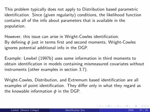
This problem typically does not apply to Distribution based parametricidentification. Since (given regularity) conditions, the likelihood functioncontains all of the info about parameters that is available in thepopulation.

However, this issue can arise in Wright-Cowles identification.By defining φ just in terms first and second moments, Wright-Cowlesignores potential additional info in the DGP.

Example: Lewbel (1997b) uses some information in third moments toobtain identification in models containing mismeasured covariates withoutinstruments (other examples in section 3.7).

Wright-Cowles, Distribution, and Extremum based identification are allexamples of point identification. They differ only in what they regard asthe knowable information φ in the DGP.


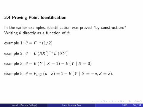
3.4 Proving Point Identification

In the earlier examples, identification was proved "by construction:"Writing θ directly as a function of φ:

example 1: θ = F−1 (1/2)

example 2: θ = E (XX ′)−1 E (XY )

example 3: θ = E (Y | X = 1)− E (Y | X = 0)

example 5: θ = FU |Z (u | z) = 1− E (Y | X = −u,Z = z).


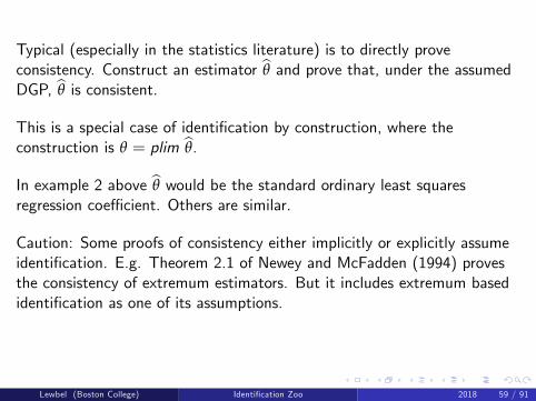
Typical (especially in the statistics literature) is to directly proveconsistency. Construct an estimator θ and prove that, under the assumedDGP, θ is consistent.

This is a special case of identification by construction, where theconstruction is θ = plim θ.

In example 2 above θ would be the standard ordinary least squaresregression coeffi cient. Others are similar.

Caution: Some proofs of consistency either implicitly or explicitly assumeidentification. E.g. Theorem 2.1 of Newey and McFadden (1994) provesthe consistency of extremum estimators. But it includes extremum basedidentification as one of its assumptions.


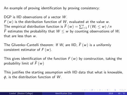
An example of proving identification by proving consistency:

DGP is IID observations of a vector W .F (w) is the distribution function of W , evaluated at the value w .The empirical distribution function is F (w) = ∑n

i=1 I (Wi ≤ w) /nF estimates the probability that W ≤ w by counting observations of Wi

that are less than w .

The Glivenko—Cantelli theorem: If Wi are IID, F (w) is a uniformlyconsistent estimator of F (w).

This gives identification of the function F (w) by construction, taking theprobability limit of F (w)

This justifies the starting assumption with IID data that what is knowable,φ, is the distribution function of W .


1. ’By construction’is the commonest way to prove identification.

Other methods are:

2. Proving true θ is the unique solution to an optimization problem.Example: maximum likelihood with a concave population objectivefunction (e.g., probit, see Haberman 1974).

3. Applying characterizations of observational equivalence in some classesof models. See Roehrig (1988) and Matzkin (2008).

4. Showing the true θ is the unique fixed point in a contraction mappingbased on M.Example: The BLP model (Berry, Levinsohn, and Pakes 1995) doesn’tquite do this, but a contraction mapping is used to prove that a necessarycondition for identification, uniqueness in the error inversion step, holds.Example: Pastorello, Patilea, and Renault (2003) use a fixed pointExtremum based identification assumption for their proposed latentbackfitting estimator.


For many examples of applying these methods to prove identification, seeMatzkin (2005, 2007, 2012).

In some cases, it is possible to empirically test for identification.

These are generally tests of extremum based identification, based on thebehavior of associated extremum based estimators.

Examples: Cragg and Donald (1993), Wright (2003), Inoue and Rossi(2011), Bravo, Escanciano, and Otsu (2012), and Arellano, Hansen, andSentana (2012).


Point identification can be defined without reference to any data at all!

Example: Model M consists of (regular) utility functions maximized undera linear budget constraint.

φ = Demand functions, θ = Indifference curves.

Revealed preference theory of Samuelson (1938,1948), Houthakker (1950),and Mas-Colell (1978) shows point identification of θ.

Note again the sense in whch definitions of identification can be a bitcircular or recursive: Start by assuming something is identified (demandfunctions) to show that something else is identified (indifference curves),given the revealed preference assumptions.

A separate question would then be when or whether demand functions canbe identified from observed data.


3.5 Common Reasons for Failure of Point Identification

Typical (somewhat overlapping) reasons identification fails or is diffi cult toattain:1. model incompleteness,2. perfect collinearity or dependence,3. nonlinearity,4. simultaneity,5. endogeneity,6. unobservability.

1. Incompleteness: variable relationships not fully specified (more aboutcompleteness and coherence later).

Example: games having multiple equilibria, without or unknownequilibrium selection rule.


2. Perfect collinearity.Let Yi = a+ bXi + cZi + ei . If Xi is linear in Zi , can’t identify a, b, c .

Perfect dependence:Can’t identify the function g (X ,Z ) = E (Y | X ,Z ) if X = h (Z ).

3. Nonlinearity can cause multiple solutions:Example: Y = (X − θ)2 + e with E (e) = 0.

Then true θ0 satisfies E(Y − (X − θ)2

)= 0

True θ0 is one of two roots of E(Y − X 2

)+ 2E (X ) θ − θ2 = 0.

Identification needs more info, e.g., maybe knowing sign of θ.Without more data, θ is locally identified.


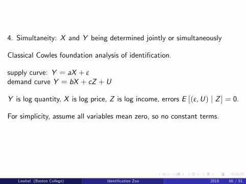
4. Simultaneity: X and Y being determined jointly or simultaneously

Classical Cowles foundation analysis of identification.

supply curve: Y = aX + εdemand curve Y = bX + cZ + U

Y is log quantity, X is log price, Z is log income, errors E [(ε,U) | Z ] = 0.

For simplicity, assume all variables mean zero, so no constant terms.


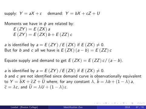
supply: Y = aX + ε demand: Y = bX + cZ + U

Moments we have in φ are related by:E (ZY ) = E (ZX ) aE (ZY ) = E (ZX ) b+ E (ZZ ) c

a is identified by a = E (ZY ) /E (ZX ) if E (ZX ) 6= 0.But for b and c all we have is E (ZX ) (a− b) = E (ZZ ) c

Equate supply and demand to get E (ZX ) = E (ZZ ) c/ (a− b).

a is identified by a = E (ZY ) /E (ZX ) if E (ZX ) 6= 0.b and c are not identified since demand curve is observationally equivalentto Y = bX + cZ + U where, for any constant λ, b = λb+ (1− λ) a,c = λc , and U = λU + (1− λ) ε.


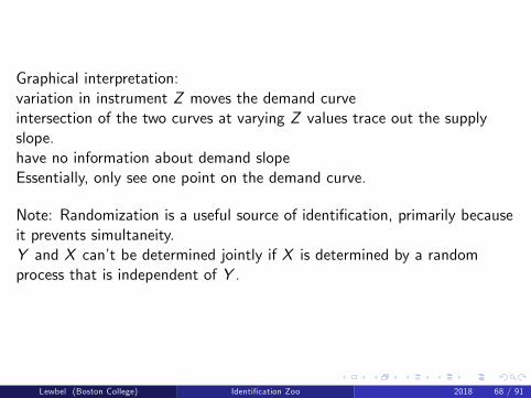
Graphical interpretation:variation in instrument Z moves the demand curveintersection of the two curves at varying Z values trace out the supplyslope.have no information about demand slopeEssentially, only see one point on the demand curve.

Note: Randomization is a useful source of identification, primarily becauseit prevents simultaneity.Y and X can’t be determined jointly if X is determined by a randomprocess that is independent of Y .


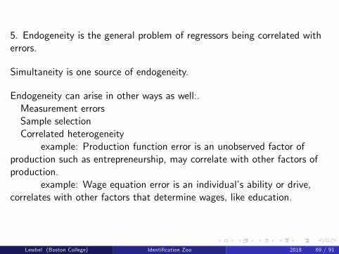
5. Endogeneity is the general problem of regressors being correlated witherrors.

Simultaneity is one source of endogeneity.

Endogeneity can arise in other ways as well:.Measurement errorsSample selectionCorrelated heterogeneity

example: Production function error is an unobserved factor ofproduction such as entrepreneurship, may correlate with other factors ofproduction.

example: Wage equation error is an individual’s ability or drive,correlates with other factors that determine wages, like education.


6. Unobservability.

Many concepts we would like to estimate are unobservable.Counterfactuals: what an untreated individual’s outcome would have beenhad they been treated.Other Examples: random utility parameters, dynamic model statevariables, production effi ciency frontiers.

Other concepts in theory observable, but diffi cult to measure.Examples: individual’s bargaining power within a household.individuals information set in a game or a dynamic optimization


Must combine assumptions and observable data to identify functions ofunobservable (or unobserved) variables.

Examples:

Point identify compensating and equivalent variation to bound (setidentify) unobserved true consumer surplus.

Assume unconfoundedness to overcome unobservability of counterfactualsin identification of ATE (Average Treatment Effects).


3.6 Control Variables

"I controlled for that."

Common response to a potential identification question (particularly insimple regressions and in Difference-in-Difference analyses). What does itmean?

Let θ be a parameter measuring the effect of one variable X on anothervariable Y .

The effect identified by the model may not equal the desired θ because ofother so-called "confounding" connections between X and Y .

Adding a control is including another variable Z in the model to fix theproblem.


The idea: Z explains the confounding relationship between X and Y .

By putting Z in the model we statistically hold Z fixed, and thereby"control" for the alternative, unintended connection between X and Y .

Fixing Z is assumed to maintain the ceteris paribus condition.

Example: X physical exercise, Y is weight gain. A control Z would beparticipant’s age.

Example: "Parallel trends" assumption in difference-in-difference models.Assumes time and group dummies Z control for all confoundingrelationships between X and Y other than the desired causal treatmenteffect.


Including a covariate Z does NOT always fix the identification problem.Can make the problem worse! Two reasons why:

1. Functional form

Unless we have a structural model of how Z affects Y , should include Z inthe model in a highly flexible (ideally nonparametric) way. Otherwise,model might be misspecified.

Including controls additively and linearly (i.e., as additional regressors in alinear regression) is a strong structural modeling assumption, even if themodel is causal like LATE or difference-in-difference. Exception is"saturated" model.


Second, bigger reason why Including a covariate Z does NOT always fixthe identification problem. Can make the problem worse:

2. Endogeneity

If Z is endogenous, fixing the omitted variable problem introducesendogeneity.

In the causal diagram literature have "confounders" and "colliders." See,e.g., Pearl (2000, 2009).

When Z is confounder, including it controls the problem.

When Z is a collider, including it can ruin identification of the causaleffect of X on Y .


Example: A wage equation

Y is wage, X is a gender dummy. Looking to identify, e.g., wagediscrimination.

Confounding problem: women may choose different occupations frommen, and occupation affects wages.

Should we include occupation Z in the model as a control?

Z is endogenous: wages that are offered to men and to women affect theiroccupation choice.

Z is a collider. Unless we have a proper instrument for Z , the coeffi cientson both X and Z will still be biased (inconsistent) in general.


Same problem can affect Difference-in-Difference models:

The dummies and other covariates in these models are supposed to becontrols for all sorts of potentially endogenous group and time relatedeffects.

But if any of these dummies or covariates are colliders (or highly correlatewith colliders), the causal interpretation of the difference-in-differenceestimand may be lost.

These issues with potential controls are closely related to the well knownBerkson (1946) and Simpson (1951) paradoxes.

Bottom line: either implicit or explicit considerations of underlyingstructure is needed to convincingly argue that covariates intended to serveas controls will actually function as they are intended.


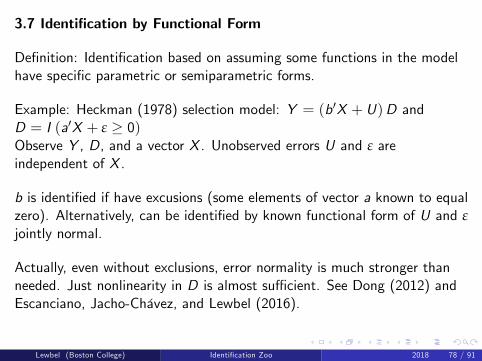
3.7 Identification by Functional Form

Definition: Identification based on assuming some functions in the modelhave specific parametric or semiparametric forms.

Example: Heckman (1978) selection model: Y = (b′X + U)D andD = I (a′X + ε ≥ 0)Observe Y , D, and a vector X . Unobserved errors U and ε areindependent of X .

b is identified if have excusions (some elements of vector a known to equalzero). Alternatively, can be identified by known functional form of U and εjointly normal.

Actually, even without exclusions, error normality is much stronger thanneeded. Just nonlinearity in D is almost suffi cient. See Dong (2012) andEscanciano, Jacho-Chávez, and Lewbel (2016).


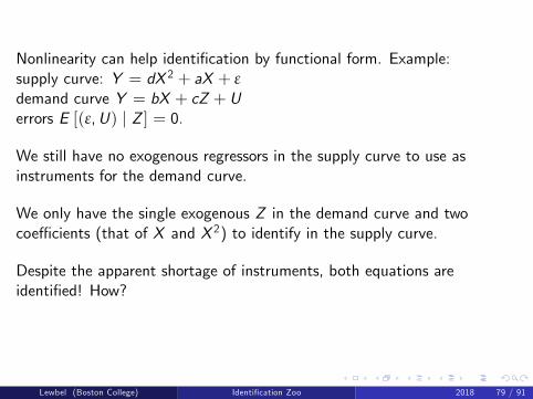
Nonlinearity can help identification by functional form. Example:supply curve: Y = dX 2 + aX + εdemand curve Y = bX + cZ + Uerrors E [(ε,U) | Z ] = 0.

We still have no exogenous regressors in the supply curve to use asinstruments for the demand curve.

We only have the single exogenous Z in the demand curve and twocoeffi cients (that of X and X 2) to identify in the supply curve.

Despite the apparent shortage of instruments, both equations areidentified! How?


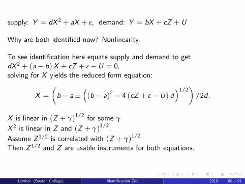
supply: Y = dX 2 + aX + ε, demand: Y = bX + cZ + U

Why are both identified now? Nonlinearity.

To see identification here equate supply and demand to getdX 2 + (a− b)X + cZ + ε− U = 0,solving for X yields the reduced form equation:

X =(b− a±

((b− a)2 − 4 (cZ + ε− U) d

)1/2)

/2d .

X is linear in (Z + γ)1/2 for some γ

X 2 is linear in Z and (Z + γ)1/2.Assume Z 1/2 is correlated with (Z + γ)1/2

Then Z 1/2 and Z are usable instruments for both equations.


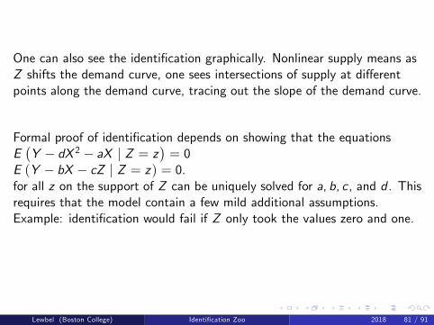
One can also see the identification graphically. Nonlinear supply means asZ shifts the demand curve, one sees intersections of supply at differentpoints along the demand curve, tracing out the slope of the demand curve.

Formal proof of identification depends on showing that the equationsE(Y − dX 2 − aX | Z = z

)= 0

E (Y − bX − cZ | Z = z) = 0.for all z on the support of Z can be uniquely solved for a, b, c, and d . Thisrequires that the model contain a few mild additional assumptions.Example: identification would fail if Z only took the values zero and one.


Idea of Identifying linear coeffi cients by exploiting nonlinearity elsewheregreatly generalizes.

Example: model Y = h (Z ′b, g (Z )) + ε and X = g (Z ) + UFunctions h and g are unknownjoint distribution of ε and U are unknown, independent of Z .

Models like these can arise with endogenous regressors or with sampleselection.

Escanciano, Jacho-Chávez, and Lewbel (2016) show that the coeffi cients band the functions h and g can generally be identified in this model.

Key requirement is linear Z ′b and nonlinear g .


Identification by functional form, another example:

Y = a+ bX + cZ + U

Assume X is endogenous (correlated with U) and have no exclusionassumption (no outside instruments). Lewbel (2012, 2018) exploitsheteroskedasticity instead of nonlinearity in the X equation to identify themodel.

Regress X = γ+ δZ + e, then let R =(Z − Z

)e. Under some

heteroskedasticity assumptions, R is a valid instrument for X .

Example assumptions that work: X is mismeasured, so U contains bothmodel and measurement error. True model error in the Y equation ishomoskedastic, e is heteroskedastic. This also works for some kinds offactor models.


Measurement error Identification by functional form:

Let Y = a+ bX + U where X has classical measurement error.Assume true X independent of model and measurement errors.

Reiersøl (1950) showed a and b are identified as long as either the true Xor the true errors are NOT normal. Normality is the worst possiblefunctional form for identification with measurement error!

Lewbel (1997b) shows, if measurement error is symmetric and true X isasymmetric, then

(X − X

)2is a valid instrument for X . Empirical

example is regression of patent counts on R&D expenditures.

Schennach and Hu (2013) show Reiersøl extends to identifyY = g (X ) + U with mismeasured X for any function g except for a fewspecific functional forms of g and of the error distributions. In thesemodels independence of the true error has strong identifying power.


Identification by functional form or by constructed instruments depends onrelatively strong modeling assumptions.

When available, better to use ’true’outside instruments (based on theorybased exclusions).

Causal inference proponents go further, accepting only randomization as avalid source of exogenous variation.


Good use of constructed instruments or identification by functional form?For testing and robustness.

In practice, one often can’t be sure if assumptions needed for outsideinstrument validity (exclusions) are satisfied.

Even with randomization, assumptions for validity, like no measurementerrors correlated with treatment, can be violated (see section 5).

For testing: can combine functional form based moments (e.g.constructed instruments) with moments based on "true" instruments toget overidentification.

Use the results for instrument validity testing, robustness checks, andeffi ciency.


Example: Y = a+ bX + cZ + U

Z is exogenous, X is endogenous, outside variable W a proposedinstrument for X , and R =

(Z − Z

)e is Lewbel’s (2012)

heteroskedasticity based constructed instrument.

2SLS using both R and W as instruments for X is overidentified - testjointly for validity of the instruments by Sargan (1958) and Hansen (1982)J-test.

If rejected, then model misspecified or an instrument is invalid. Else haveincreased confidence in both W and R. Both might then be used inestimation to maximize effi ciency.

Or just check robustness of estimated effects to various possible true andconstructed instruments.

More confidence that estimated effects are reliable if different sources ofidentification (randomization, exclusions, constructed moments) all agree.


3.8 Over, Under, and Exact Identification, Rank and Orderconditions.

Models are often contain sets of equalities involving θ, e.g., momentconditions like E [g (W , θ)] = 0,where W is data and g are known functions.

Many estimators are based on moment equalities: OLS, 2SLS, GMM, andfirst order conditions from extremum estimators like MLE score functions.

Suppose identification of a vector θ is based on equalities.θ is exactly identified if removing any one equality loses identification,θ is overidentified if θ can still be identified after removing one or moreequalities.θ is underidentified if don’t have enough equalities to identify θ.


For θ a J−vector, usually need J equations to exactly identify θ.Number of equations equal number of unknowns is the order condition foridentification.

In linear models, identification also requires a rank condition on the matrixthat θ multiplies.

General rank conditions for nonlinear models exist, based on the rank ofrelevant Jacobian matrices. See Fisher (1959, 1966), Rothenberg (1971),Sargan (1983), Bekker and Wansbeek (2001), and section 8.1 later onlocal identification.

Often satisfying the order condition may suffi ce for generic identification(see section 8.2 later).


When parameters are overidentified, can usually test validity of themoments used for identification.

Intuitively, could estimate the J vector θ using different combinations of Jmoments, and test if the resulting estimates of θ all equal each other.

In practice, more powerful tests exploit all the moments simultaneously.E.g. Sargan (1958) and Hansen (1982) J-test.

Arellano, Hansen, and Sentana (2012) discuss testing forunderidentification.

Terminology defined in this subsection is generally from the Cowlesfoundation era, e.g., the term ’order condition’dates back at least toKoopmans (1949).

Above terminology is for θ a vector, not a function. Chen and Santos(2015) extend to define a notion of semiparametric local overidentification.


End of Part 1



5. Causal Reduced Form vs Structural Model Identification


6. Identification of Functions and Sets

7. Limited Forms of Identification

8. Identification Concepts that Affect Inference

9. Conclusions


the identi–cation zoo - meanings of identi–cation in ... · continued next slide ... formal...

Documents