the gradient - ittcjstiles/220/handouts/section_2_5_the_calculus_of... · taking the gradient of...

09/16/05 The Gradient.doc 1/8

Jim Stiles The Univ. of Kansas Dept. of EECS

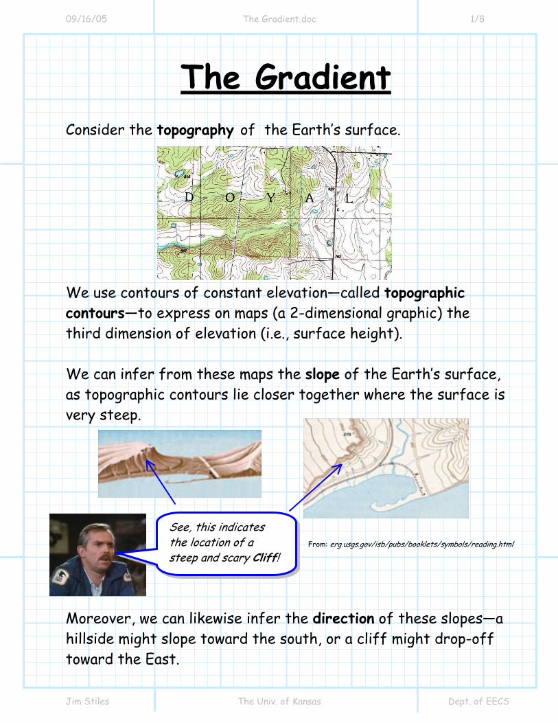
The Gradient Consider the topography of the Earth’s surface. We use contours of constant elevation—called topographic contours—to express on maps (a 2-dimensional graphic) the third dimension of elevation (i.e., surface height). We can infer from these maps the slope of the Earth’s surface, as topographic contours lie closer together where the surface is very steep. Moreover, we can likewise infer the direction of these slopes—a hillside might slope toward the south, or a cliff might drop-off toward the East.

From: erg.usgs.gov/isb/pubs/booklets/symbols/reading.html

See, this indicates the location of a steep and scary Cliff!



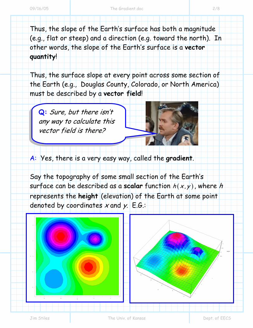
Thus, the slope of the Earth’s surface has both a magnitude (e.g., flat or steep) and a direction (e.g. toward the north). In other words, the slope of the Earth’s surface is a vector quantity! Thus, the surface slope at every point across some section of the Earth (e.g., Douglas County, Colorado, or North America) must be described by a vector field! A: Yes, there is a very easy way, called the gradient. Say the topography of some small section of the Earth’s surface can be described as a scalar function ( ),h x y , where h represents the height (elevation) of the Earth at some point denoted by coordinates x and y. E.G.:

Q: Sure, but there isn’t any way to calculate this vector field is there?

-4

-2

0

2

4

x

-4

-2

0

2

4

y

-0.5

0

0.5

1

height

-4

-2

0

2

4

x

-0.5

0

0.5

1

height

-4 -2 0 2 4x

-4

-2

0

2

4

y



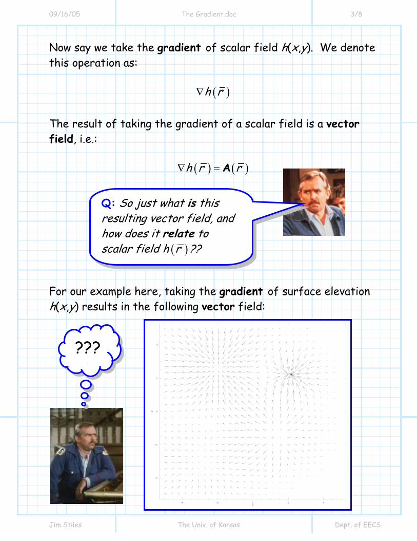
Now say we take the gradient of scalar field h(x,y). We denote this operation as:

( )h r∇

The result of taking the gradient of a scalar field is a vector field, i.e.:

( ) ( )h r r∇ = A For our example here, taking the gradient of surface elevation h(x,y) results in the following vector field:

Q: So just what is this resulting vector field, and how does it relate to scalar field ( )h r ??

-4 -2 0 2 4x

-4

-2

0

2

4

y

????



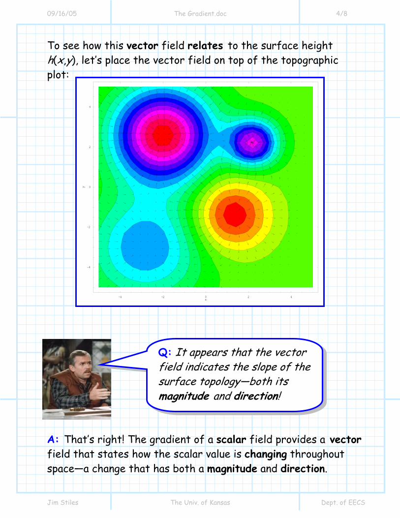
To see how this vector field relates to the surface height h(x,y), let’s place the vector field on top of the topographic plot: A: That’s right! The gradient of a scalar field provides a vector field that states how the scalar value is changing throughout space—a change that has both a magnitude and direction.

-4 -2 0 2 4x

-4

-2

0

2

4

y

Q: It appears that the vector field indicates the slope of the surface topology—both its magnitude and direction!



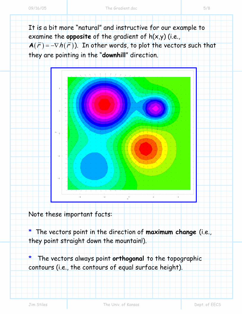
It is a bit more “natural” and instructive for our example to examine the opposite of the gradient of h(x,y) (i.e., ( ) ( )r h r= −∇A ). In other words, to plot the vectors such that

they are pointing in the “downhill” direction. Note these important facts: * The vectors point in the direction of maximum change (i.e., they point straight down the mountain!). * The vectors always point orthogonal to the topographic contours (i.e., the contours of equal surface height).

-4 -2 0 2 4x

-4

-2

0

2

4

y



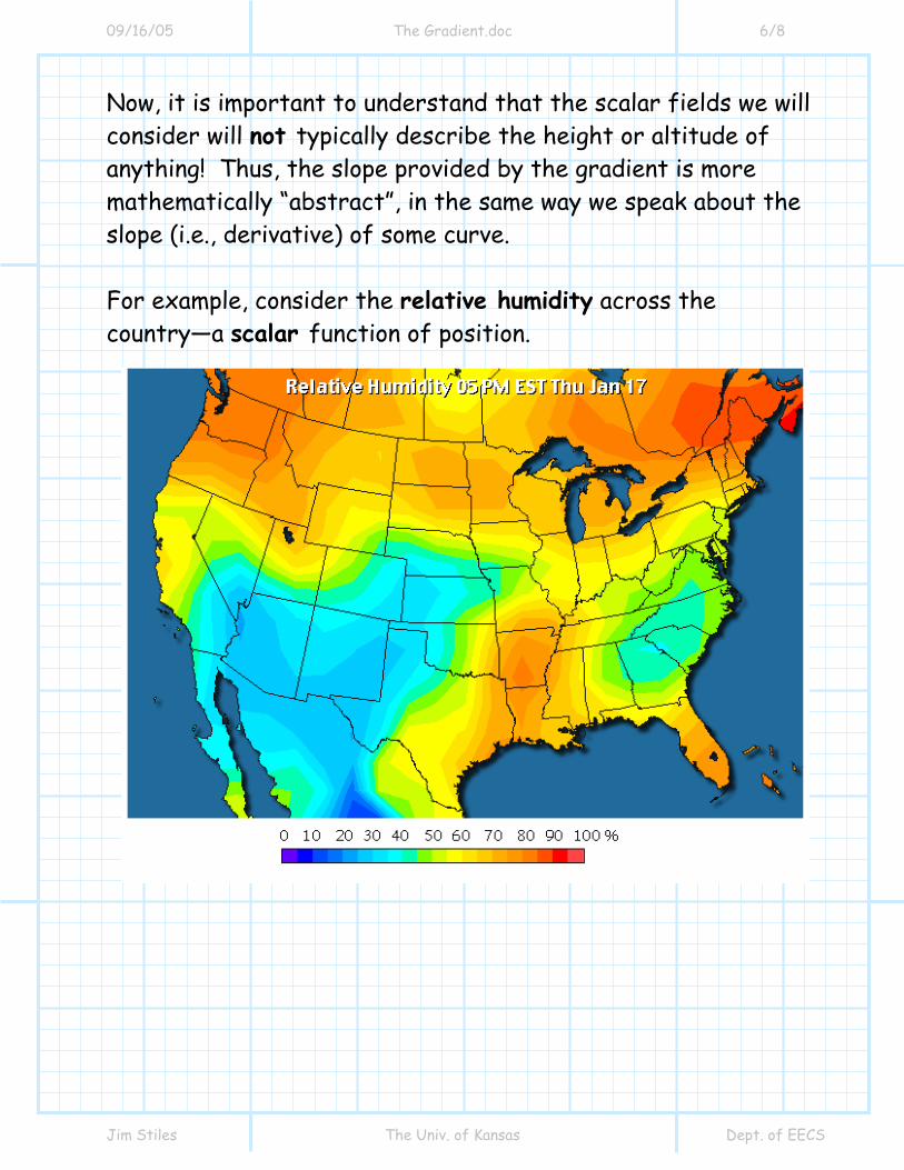
Now, it is important to understand that the scalar fields we will consider will not typically describe the height or altitude of anything! Thus, the slope provided by the gradient is more mathematically “abstract”, in the same way we speak about the slope (i.e., derivative) of some curve. For example, consider the relative humidity across the country—a scalar function of position.



If we travel in some directions, we will find that the humidity quickly changes. But if we travel in other directions, the humidity will change not at all.

Q: Say we are located at some point (e.g., Lawrence, KS; Albuquerque, N M; or Ann Arbor, MI), how can we determine the direction where we will experience the greatest change in humidity ?? Also, how can we determine what that change will be ?? A: The answer to both questions is to take the gradient of the scalar field that represents humidity!

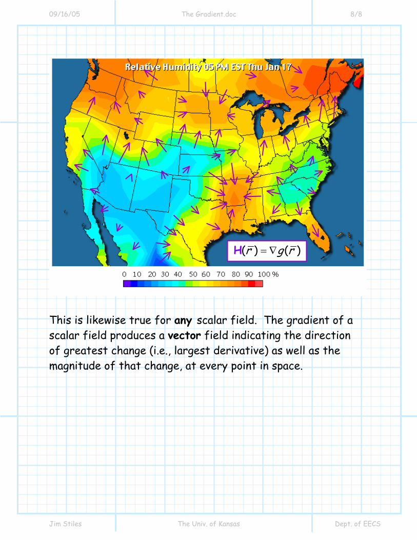
If ( )rg is the scalar field that represents the humidity across the country, then we can form a vector field ( )rH by taking the gradient of ( )rg :

( ) ( )r rg= ∇H

This vector field indicates the direction of greatest humidity change (i.e., the direction where the derivative is the largest), as well as the magnitude of that change, at every point in the country!



This is likewise true for any scalar field. The gradient of a scalar field produces a vector field indicating the direction of greatest change (i.e., largest derivative) as well as the magnitude of that change, at every point in space.

( ) ( )r g r= ∇H

09/16/05 The Gradient Operator in Coordinate Systems.doc 1/2


The Gradient Operator in Coordinate Systems

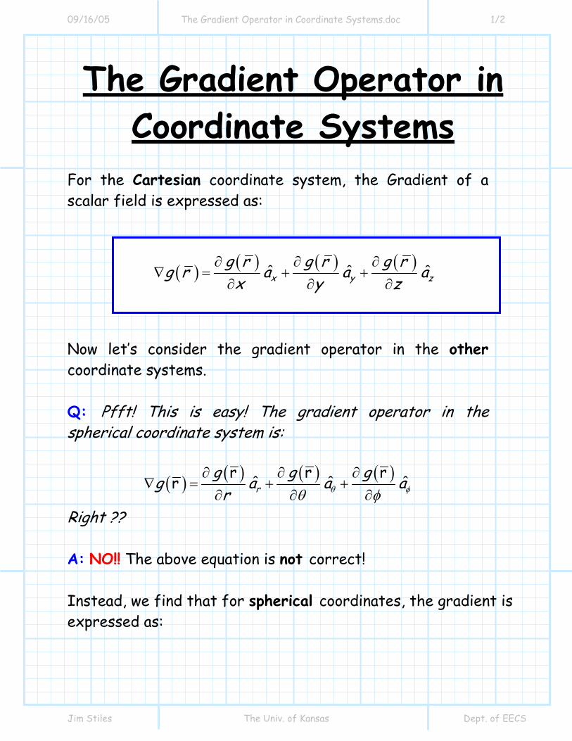
For the Cartesian coordinate system, the Gradient of a scalar field is expressed as:

( ) ( ) ( ) ( )ˆ ˆ ˆx y zg r g r g rg r a a a

x y z∂ ∂ ∂

∇ = + +∂ ∂ ∂

Now let’s consider the gradient operator in the other coordinate systems. Q: Pfft! This is easy! The gradient operator in the spherical coordinate system is:

( ) ( ) ( ) ( )ˆ ˆ ˆr r rr r

g g gg a a ar θ φθ φ

∂ ∂ ∂∇ = + +

∂ ∂ ∂

Right ?? A: NO!! The above equation is not correct!

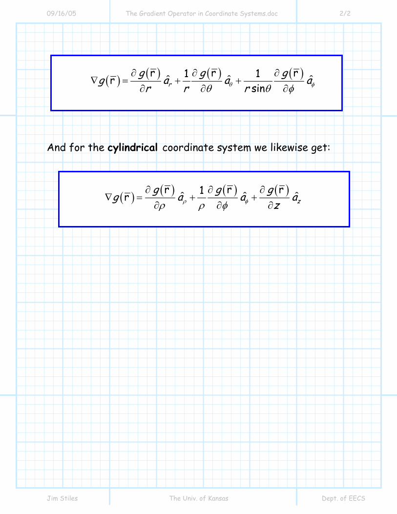
Instead, we find that for spherical coordinates, the gradient is expressed as:

09/16/05 The Gradient Operator in Coordinate Systems.doc 2/2


( ) ( ) ( ) ( )ˆ ˆ ˆr r r1 1rsinr

g g gg a a ar r rθ φθ θ φ

∂ ∂ ∂∇ = + +

∂ ∂ ∂

And for the cylindrical coordinate system we likewise get:

( ) ( ) ( ) ( )ˆ ˆ ˆr r r1r zg g gg a a a

zρ φρ ρ φ∂ ∂ ∂

∇ = + +∂ ∂ ∂

09/16/05 The Conservative Vector Field.doc 1/4


The Conservative Vector Field

Of all possible vector fields ( )rA , there is a subset of vector fields called conservative fields. A conservative vector field is a vector field that can be expressed as the gradient of some scalar field ( )rg :

( ) ( )r rg= ∇C

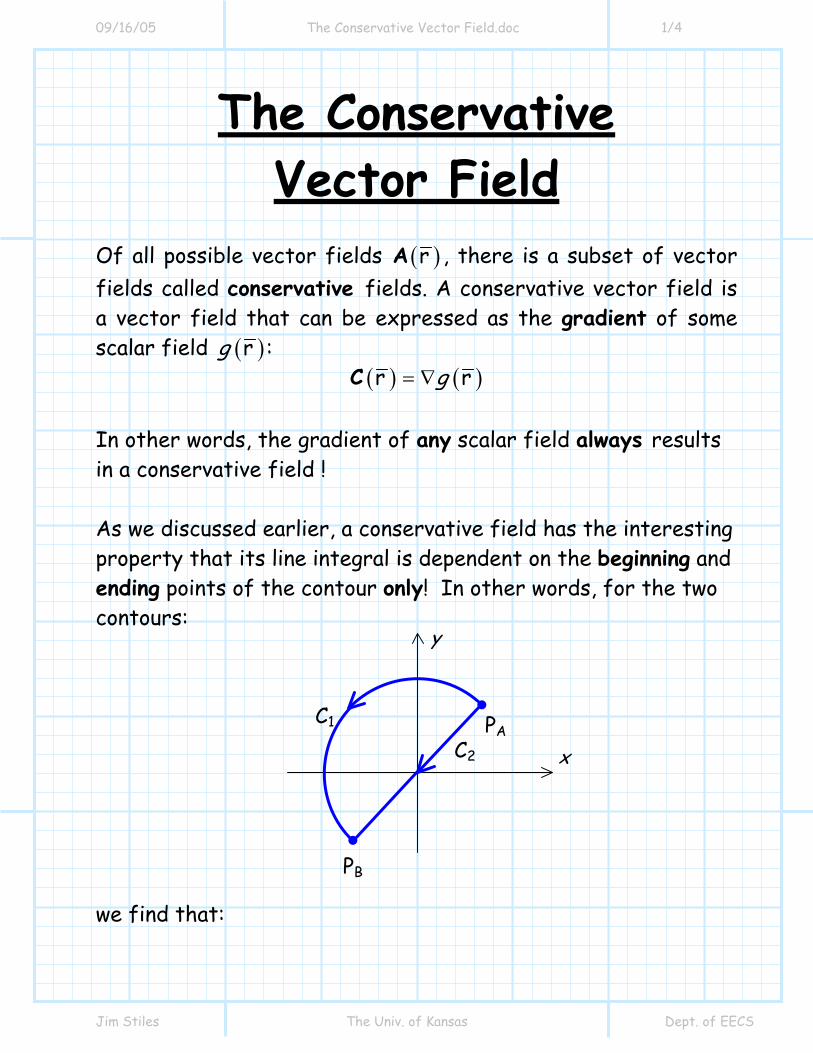
In other words, the gradient of any scalar field always results in a conservative field ! As we discussed earlier, a conservative field has the interesting property that its line integral is dependent on the beginning and ending points of the contour only! In other words, for the two contours: we find that:

PA

y

x

C1 C2

PB



( ) ( )

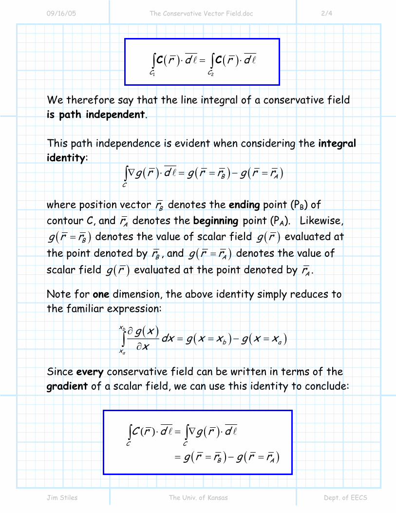
1 2C Cr d r d⋅ = ⋅∫ ∫C C

We therefore say that the line integral of a conservative field is path independent.

This path independence is evident when considering the integral identity:

( ) ( ) ( )B AC

g r d g r r g r r∇ ⋅ = = − =∫

where position vector Br denotes the ending point (PB) of contour C, and Ar denotes the beginning point (PA). Likewise, ( )Bg r r= denotes the value of scalar field ( )g r evaluated at

the point denoted by Br , and ( )Ag r r= denotes the value of scalar field ( )g r evaluated at the point denoted by Ar .

Note for one dimension, the above identity simply reduces to the familiar expression:

( ) ( ) ( )b

a

x

b ax

g x dx g x x g x xx

∂= = − =

∂∫

Since every conservative field can be written in terms of the gradient of a scalar field, we can use this identity to conclude:

( )

( ) ( )

( )C C

B A

C r d g r d

g r r g r r

⋅ = ∇ ⋅

= = − =

∫ ∫



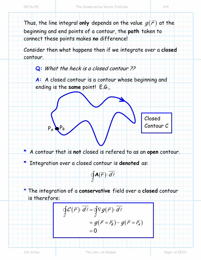
Thus, the line integral only depends on the value ( )g r at the beginning and end points of a contour, the path taken to connect these points makes no difference!

Consider then what happens then if we integrate over a closed contour.

Q: What the heck is a closed contour ??

A: A closed contour is a contour whose beginning and ending is the same point! E.G.,

* A contour that is not closed is refered to as an open contour.

* Integration over a closed contour is denoted as:

( ) ⋅∫C

drA

* The integration of a conservative field over a closed contour is therefore:

( ) ( )

( ) ( )0

C C

B A

C r d g r d

g r r g r r

⋅ = ∇ ⋅

= = − =

=

∫ ∫

PA PB Closed Contour C



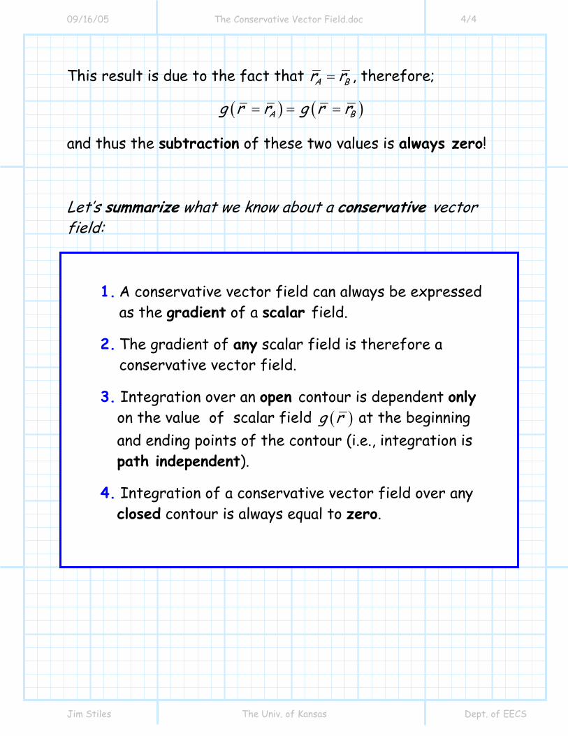
This result is due to the fact that =A Br r , therefore;

( ) ( )A Bg r r g r r= = =

and thus the subtraction of these two values is always zero!

Let’s summarize what we know about a conservative vector field:

1. A conservative vector field can always be expressed as the gradient of a scalar field.

2. The gradient of any scalar field is therefore a conservative vector field.

3. Integration over an open contour is dependent only on the value of scalar field ( )g r at the beginning and ending points of the contour (i.e., integration is path independent).

4. Integration of a conservative vector field over any closed contour is always equal to zero.

9/16/2005 Example Line Integrals of Conservative Fields .doc 1/2


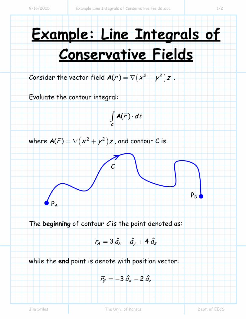
Example: Line Integrals of Conservative Fields

Consider the vector field ( )2 2( )r x y z= ∇ +A . Evaluate the contour integral:

( )C

r d⋅∫ A

where ( )2 2( )r x y z= ∇ +A , and contour C is: The beginning of contour C is the point denoted as:

ˆ ˆ ˆ3 4A x y zr a a a= − +

while the end point is denote with position vector:

= − −ˆ ˆ3 2x zBr a a

C

PA PB

9/16/2005 Example Line Integrals of Conservative Fields .doc 2/2


Note that ordinarily, this would be an impossible problem for us to do! But, we note that vector field ( )rA is conservative, therefore:

( )

( ) ( )

( )C C

B A

A r d g r d

g r r g r r

⋅ = ∇ ⋅

= = − =

∫ ∫

For this problem, it is evident that:

( )2 2( )g r x y z= +

Therefore, ( )Ag r r= is the scalar field evaluated at x = 3, y = -1, z = 4; while ( )Bg r r= is the scalar field evaluated at at x = -3, y = 0, z = -2.

( ) ( )( )2 2( ) 3 1 4 40Ag r r= = + − =

( ) ( )( )( )2 2( ) 3 0 2 18Bg r r= = − + − = −

Therefore:

( )

( ) ( )

( )

18 4058

C C

B A

A r d g r d

g r r g r r

⋅ = ∇ ⋅

= = − =

= − −= −

∫ ∫

9/16/2005 The Divergence of a Vector Field.doc 1/8


The Divergence of a Vector Field

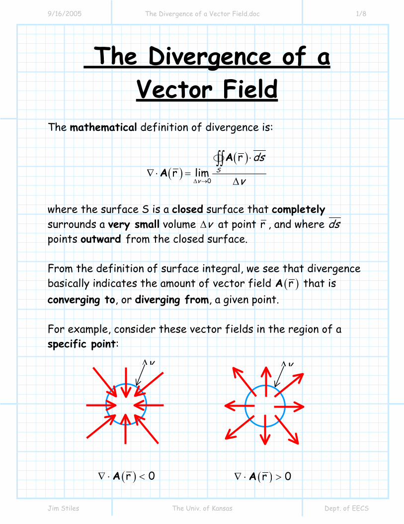
The mathematical definition of divergence is:

( )( )

∆ →

⋅∇ ⋅ =

∆

∫∫S

v

ds

v0

rr lim

AA

where the surface S is a closed surface that completely surrounds a very small volume v∆ at point r , and where ds points outward from the closed surface. From the definition of surface integral, we see that divergence basically indicates the amount of vector field ( )rA that is converging to, or diverging from, a given point. For example, consider these vector fields in the region of a specific point:

( )r 0∇ ⋅ >A ( )r 0∇ ⋅ <A

v∆v∆



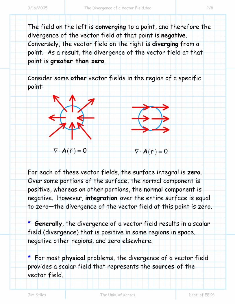
The field on the left is converging to a point, and therefore the divergence of the vector field at that point is negative. Conversely, the vector field on the right is diverging from a point. As a result, the divergence of the vector field at that point is greater than zero. Consider some other vector fields in the region of a specific point: For each of these vector fields, the surface integral is zero. Over some portions of the surface, the normal component is positive, whereas on other portions, the normal component is negative. However, integration over the entire surface is equal to zero—the divergence of the vector field at this point is zero. * Generally, the divergence of a vector field results in a scalar field (divergence) that is positive in some regions in space, negative other regions, and zero elsewhere. * For most physical problems, the divergence of a vector field provides a scalar field that represents the sources of the vector field.

( )r 0∇ ⋅ =A ( )r 0∇ ⋅ =A



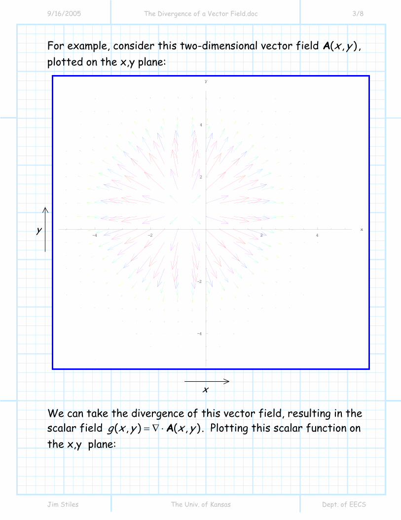
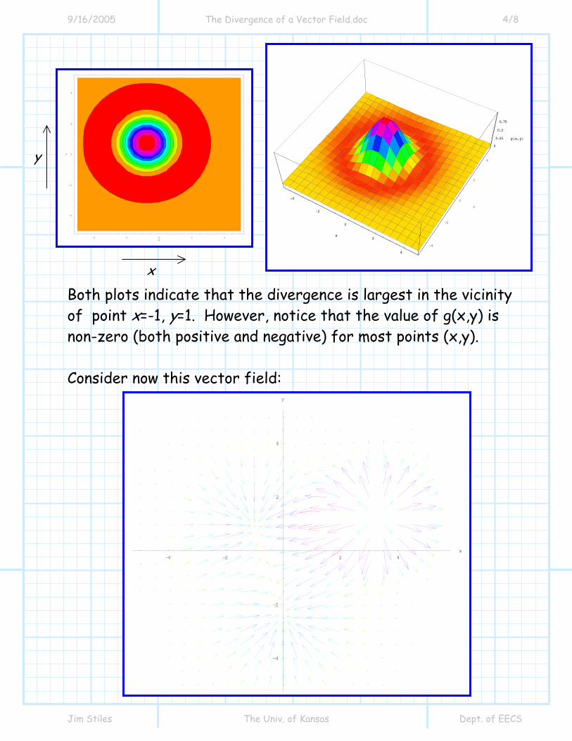
For example, consider this two-dimensional vector field ( , )x yA , plotted on the x,y plane: We can take the divergence of this vector field, resulting in the scalar field ( , ) ( , )g x y x y= ∇ ⋅A . Plotting this scalar function on the x,y plane:

x

y -4 -2 2 4

x

-4

-2

2

4

y



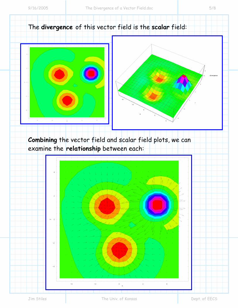
Both plots indicate that the divergence is largest in the vicinity of point x=-1, y=1. However, notice that the value of g(x,y) is non-zero (both positive and negative) for most points (x,y). Consider now this vector field:

y

x

-4 -2 2 4x

-4

-2

2

4

y

-4 -2 0 2 4x

-4

-2

0

2

4

y

-4

-2

0

2

4

x

-4

-2

0

2

4

y

0

0.25

0.5

0.75

gHx,yL

-4

-2

0

2

4

x

0

0.25

0.5

0.75

gHx,yL



The divergence of this vector field is the scalar field: Combining the vector field and scalar field plots, we can examine the relationship between each:

-4 -2 0 2 4x

-4

-2

0

2

4

y

-4

-2

0

2

4

x

-4

-2

0

2

4

y

0

1

divergence

-4

-2

0

2

4

x

0

1

divergence

-4 -2 0 2 4x

-4

-2

0

2

4

y



Look closely! Although the relationship between the scalar field and the vector field may appear at first to be the same as with the gradient operator, the two relationships are very different. Remember:

a) gradient produces a vector field that indicates the change in the original scalar field, whereas:

b) divergence produces a scalar field that indicates some change (i.e., divergence or convergence) of the original vector field.

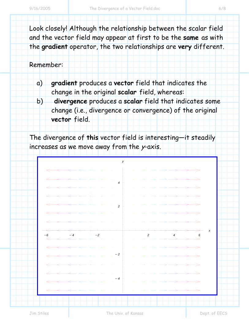
The divergence of this vector field is interesting—it steadily increases as we move away from the y-axis.

-6 - 4 -2 2 4 6x

- 4

- 2

2

4

y



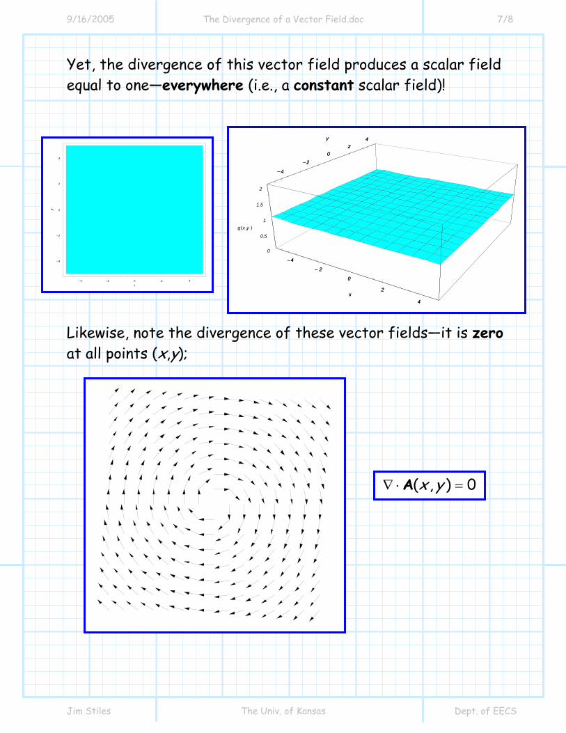
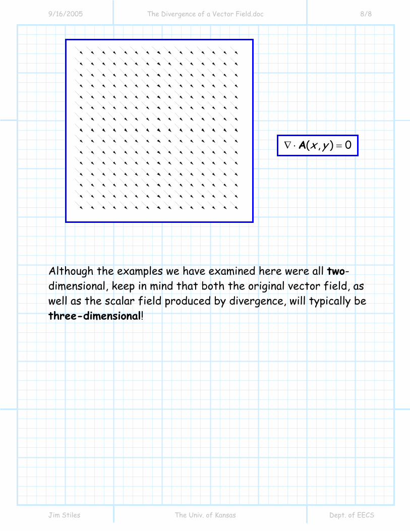
Yet, the divergence of this vector field produces a scalar field equal to one—everywhere (i.e., a constant scalar field)! Likewise, note the divergence of these vector fields—it is zero at all points (x,y);

- 4 -2 0 2 4x

-4

-2

0

2

4

y

-4

- 2

0

2

4x

-4

-20

24y

0

0.5

1

1.5

2

gHx,y L

-4

- 2

0

2

4x

-4

-20

24y

( , ) 0x y∇ ⋅ =A



Although the examples we have examined here were all two-dimensional, keep in mind that both the original vector field, as well as the scalar field produced by divergence, will typically be three-dimensional!

( , ) 0x y∇ ⋅ =A

9/16/2005 The Divergence in Coordinate Systems.doc 1/2


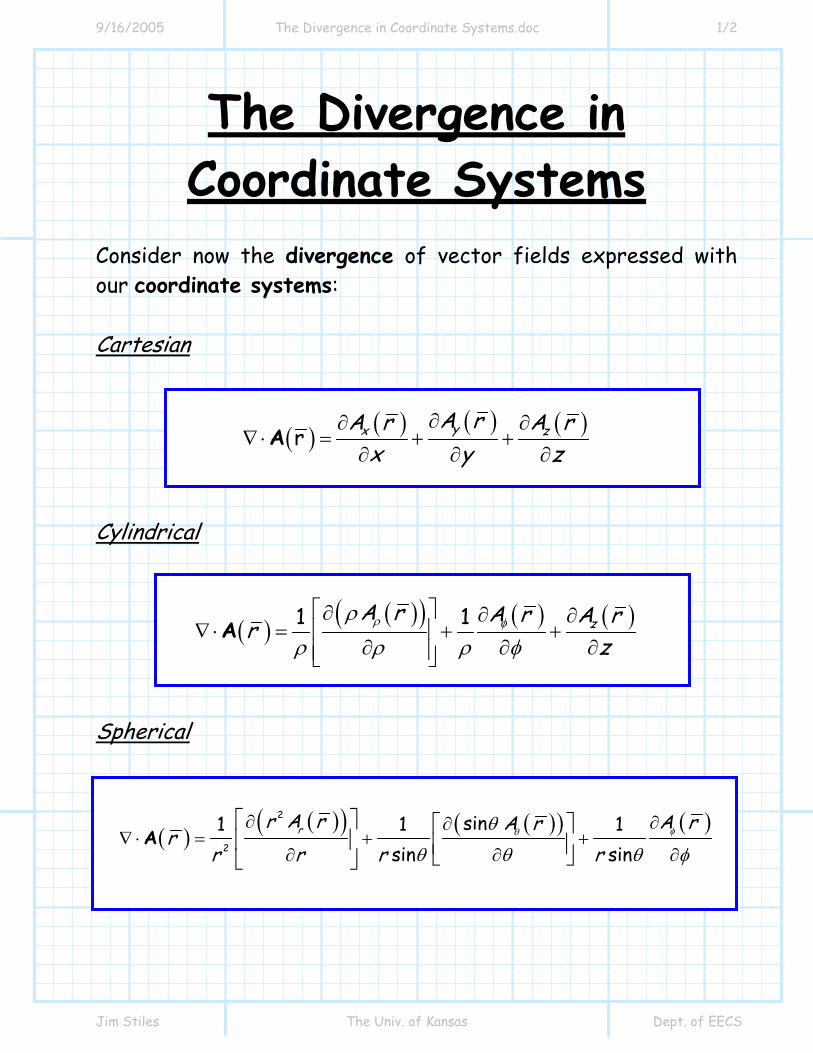
The Divergence in Coordinate Systems

Consider now the divergence of vector fields expressed with our coordinate systems: Cartesian

( ) ( ) ( ) ( )r yx zA rA r A rx y z

∂∂ ∂∇ ⋅ = + +

∂ ∂ ∂A

Cylindrical

( )( )( ) ( ) ( )1 1 zA r A r A rr

zρ φρ

ρ ρ ρ φ

⎡ ⎤∂ ∂ ∂∇ ⋅ = + +⎢ ⎥

∂ ∂ ∂⎢ ⎥⎣ ⎦A

Spherical

( )( )( ) ( )( ) ( )2

2

sin1 1 1sin sin

rr A r A rA rr

r r r rφθθ

θ θ θ φ

∂ ∂∂∇ ⋅ = + +

∂ ∂ ∂

⎡ ⎤ ⎡ ⎤⎢ ⎥ ⎢ ⎥⎣ ⎦⎣ ⎦

A

9/16/2005 The Divergence in Coordinate Systems.doc 2/2


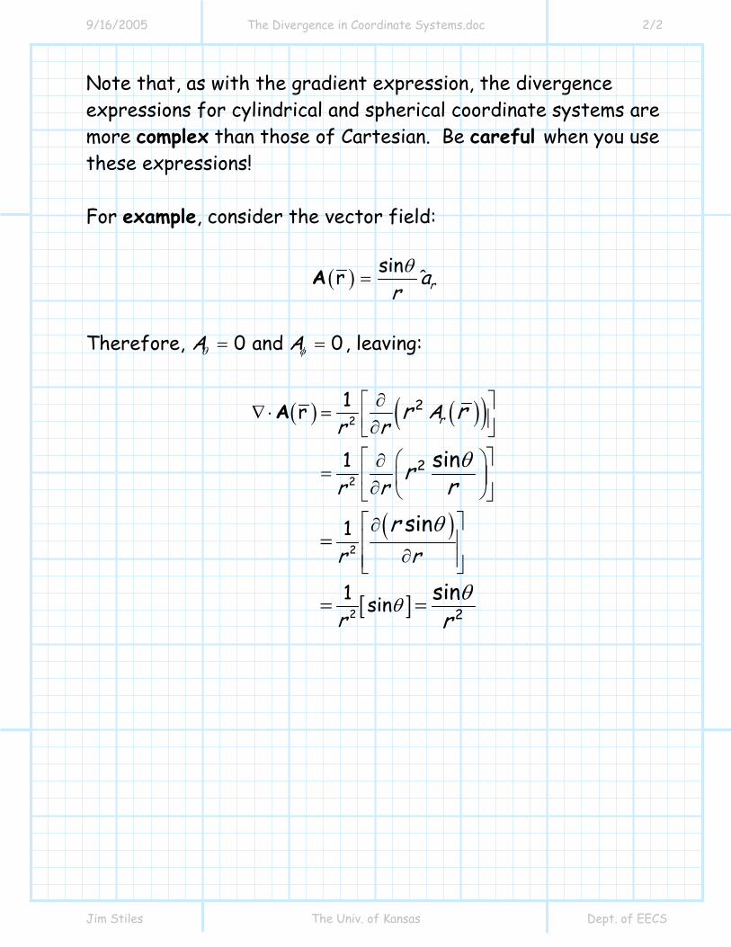
Note that, as with the gradient expression, the divergence expressions for cylindrical and spherical coordinate systems are more complex than those of Cartesian. Be careful when you use these expressions! For example, consider the vector field:

( ) sinr ˆ rarθ

=A

Therefore, 0 and 0A Aθ φ= = , leaving:

( ) ( )( )

( )

[ ]

2

2

2

2

2

2

2

1r

1

1

1 sin

sin

sin

sin

rAr r

r r

r r

r

r r

r rr

rθ

θ

θ

θ

∂⎡ ⎤∇ ⋅ = ⎢ ⎥∂⎣ ⎦⎡ ⎤⎛ ⎞∂

= ⎢ ⎥⎜ ⎟∂ ⎝ ⎠⎣ ⎦⎡ ⎤∂⎢ ⎥

∂⎢ ⎥⎣ ⎦=

= =

A

9/16/2005 The Divergence Theorem.doc 1/2


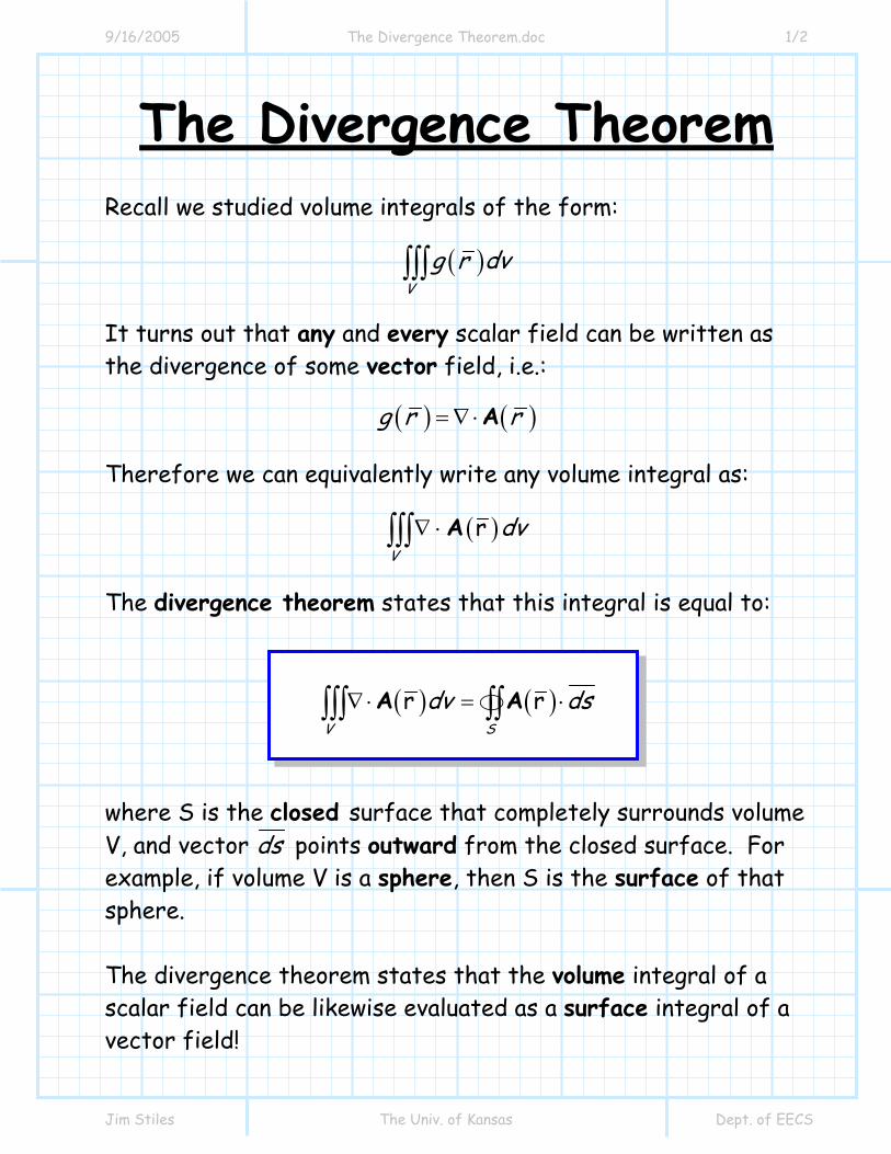
The Divergence Theorem Recall we studied volume integrals of the form:

( )V

g r dv∫∫∫

It turns out that any and every scalar field can be written as the divergence of some vector field, i.e.:

( ) ( )g r r= ∇ ⋅A

Therefore we can equivalently write any volume integral as:

( )rV

dv∇ ⋅∫∫∫ A

The divergence theorem states that this integral is equal to:

( ) ( )∇ ⋅ = ⋅∫∫∫ ∫∫V S

dv dsr rA A

where S is the closed surface that completely surrounds volume V, and vector ds points outward from the closed surface. For example, if volume V is a sphere, then S is the surface of that sphere. The divergence theorem states that the volume integral of a scalar field can be likewise evaluated as a surface integral of a vector field!

9/16/2005 The Divergence Theorem.doc 2/2


-4 - 2 0 2 4

-4

-2

0

2

4

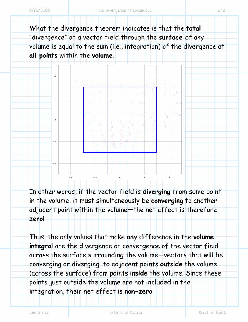
What the divergence theorem indicates is that the total “divergence” of a vector field through the surface of any volume is equal to the sum (i.e., integration) of the divergence at all points within the volume. In other words, if the vector field is diverging from some point in the volume, it must simultaneously be converging to another adjacent point within the volume—the net effect is therefore zero! Thus, the only values that make any difference in the volume integral are the divergence or convergence of the vector field across the surface surrounding the volume—vectors that will be converging or diverging to adjacent points outside the volume (across the surface) from points inside the volume. Since these points just outside the volume are not included in the integration, their net effect is non-zero!

9/16/2005 The Curl of a Vector Field.doc 1/7


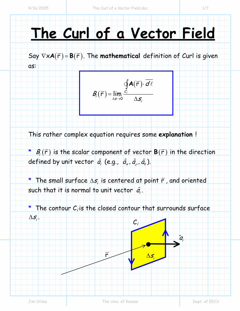
The Curl of a Vector Field Say ( ) ( )x r r∇ =A B . The mathematical definition of Curl is given as:

( )( )

0

rr lim iC

i s i

dB

s∆ →

⋅

=∆

∫A

This rather complex equation requires some explanation ! * ( )riB is the scalar component of vector ( )rB in the direction defined by unit vector ia (e.g., ˆ ˆ ˆ, ,xa a aρ θ ). * The small surface is∆ is centered at point r , and oriented such that it is normal to unit vector ia . * The contour Ci is the closed contour that surrounds surface

is∆ .

Ci

is∆

ˆ ia

r



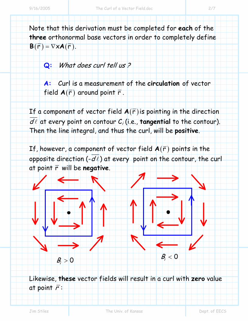
Note that this derivation must be completed for each of the three orthonormal base vectors in order to completely define ( ) ( )r x r= ∇B A .

Q: What does curl tell us ? A: Curl is a measurement of the circulation of vector field ( )rA around point r .

If a component of vector field ( )rA is pointing in the direction d at every point on contour Ci (i.e., tangential to the contour). Then the line integral, and thus the curl, will be positive. If, however, a component of vector field ( )rA points in the opposite direction (-d ) at every point on the contour, the curl at point r will be negative.

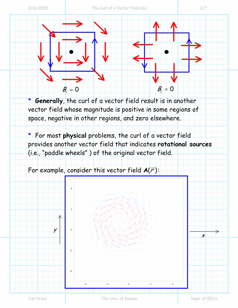
Likewise, these vector fields will result in a curl with zero value at point r :

0iB > 0iB <



* Generally, the curl of a vector field result is in another vector field whose magnitude is positive in some regions of space, negative in other regions, and zero elsewhere. * For most physical problems, the curl of a vector field provides another vector field that indicates rotational sources (i.e., “paddle wheels” ) of the original vector field. For example, consider this vector field ( )rA :

0iB = 0iB =

x y

-4 - 2 0 2 4

-4

-2

0

2

4



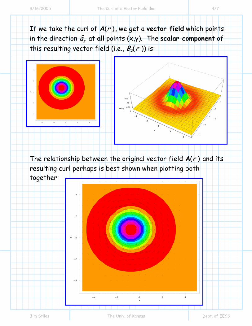
If we take the curl of ( )rA , we get a vector field which points in the direction za at all points (x,y). The scalar component of this resulting vector field (i.e., Bz(r )) is: The relationship between the original vector field ( )rA and its resulting curl perhaps is best shown when plotting both together:

-4 -2 0 2 4x

-4

-2

0

2

4

y

-4

-2

0

2

4

x

- 4

-2

0

2

4

y

0

0.25

0.5

0.75

Ax Hx,y L

-4

-2

0

2

4

x

-4 -2 0 2 4x

-4

-2

0

2

4

y



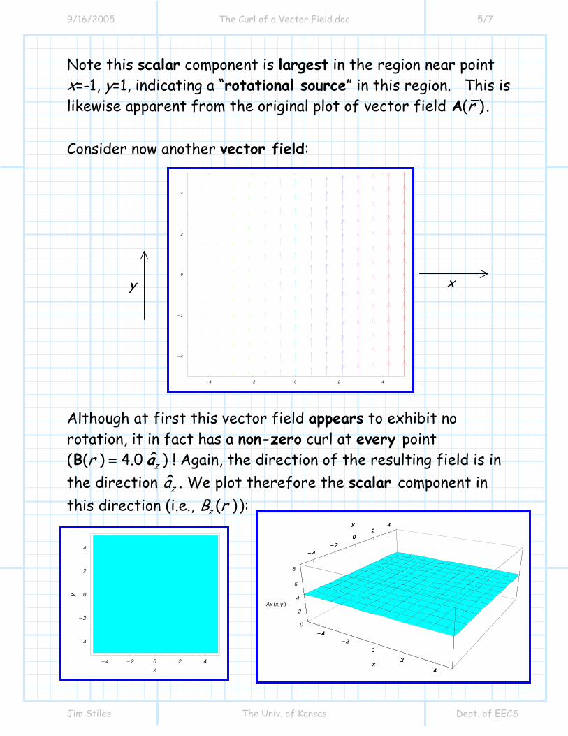
Note this scalar component is largest in the region near point x=-1, y=1, indicating a “rotational source” in this region. This is likewise apparent from the original plot of vector field ( )rA . Consider now another vector field: Although at first this vector field appears to exhibit no rotation, it in fact has a non-zero curl at every point ( ˆ( ) 4.0 zr =B a ) ! Again, the direction of the resulting field is in the direction za . We plot therefore the scalar component in this direction (i.e., ( )zB r ):

x y

-4 - 2 0 2 4

-4

-2

0

2

4

-4 -2 0 2 4x

-4

-2

0

2

4

y

-4-2

0

2

4x

-4-2

02

4y

0

2

4

6

8

Ax Hx,y L

-4-2

0

2

4x

-4-2

02

4y



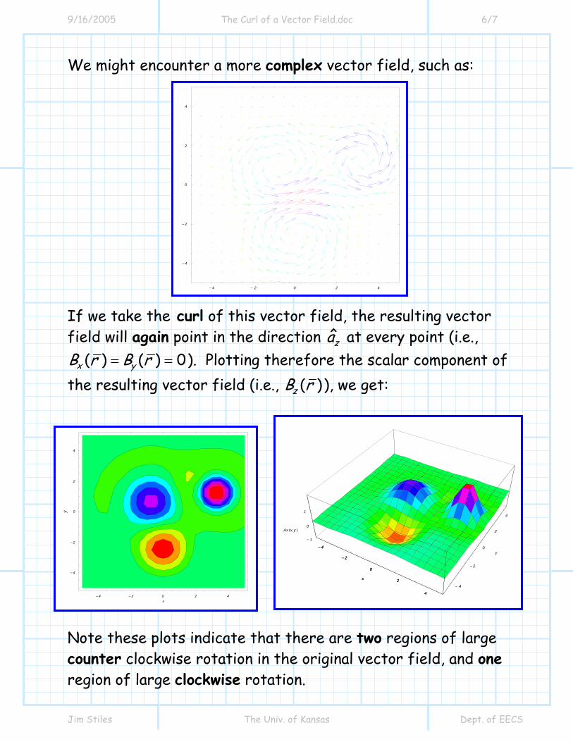
We might encounter a more complex vector field, such as: If we take the curl of this vector field, the resulting vector field will again point in the direction za at every point (i.e.,

( ) ( ) 0x yB r B r= = ). Plotting therefore the scalar component of the resulting vector field (i.e., ( )zB r ), we get: Note these plots indicate that there are two regions of large counter clockwise rotation in the original vector field, and one region of large clockwise rotation.

-4 - 2 0 2 4

-4

-2

0

2

4

-4 -2 0 2 4x

-4

-2

0

2

4

y

-4

-2

0

2

4

x

- 4

-2

0

2

4

y

-1

0

1

Ax Hx,y L

-4

-2

0

2

4

x



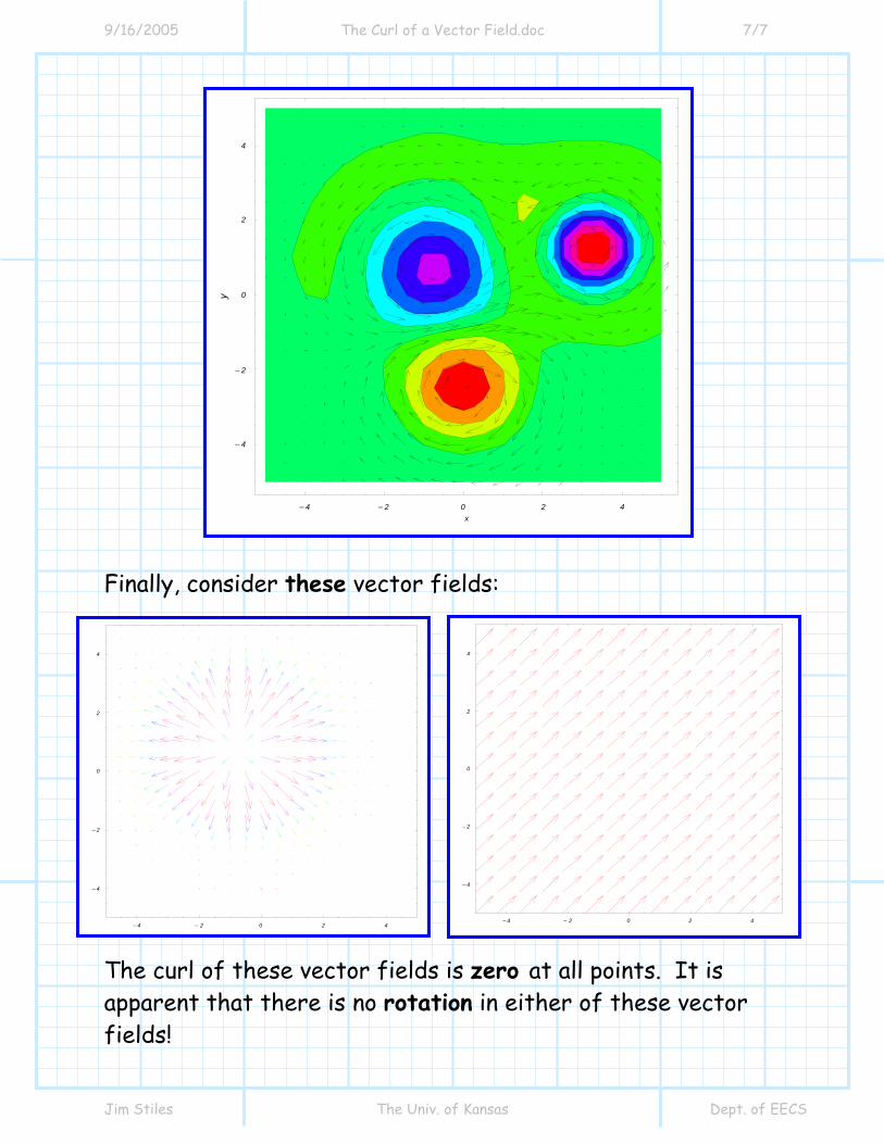
Finally, consider these vector fields: The curl of these vector fields is zero at all points. It is apparent that there is no rotation in either of these vector fields!

-4 -2 0 2 4x

-4

-2

0

2

4

y

-4 - 2 0 2 4

-4

-2

0

2

4

-4 - 2 0 2 4

-4

-2

0

2

4

9/16/2005 Curl in Cylindrical and Spherical Coordinate Systems.doc 1/2


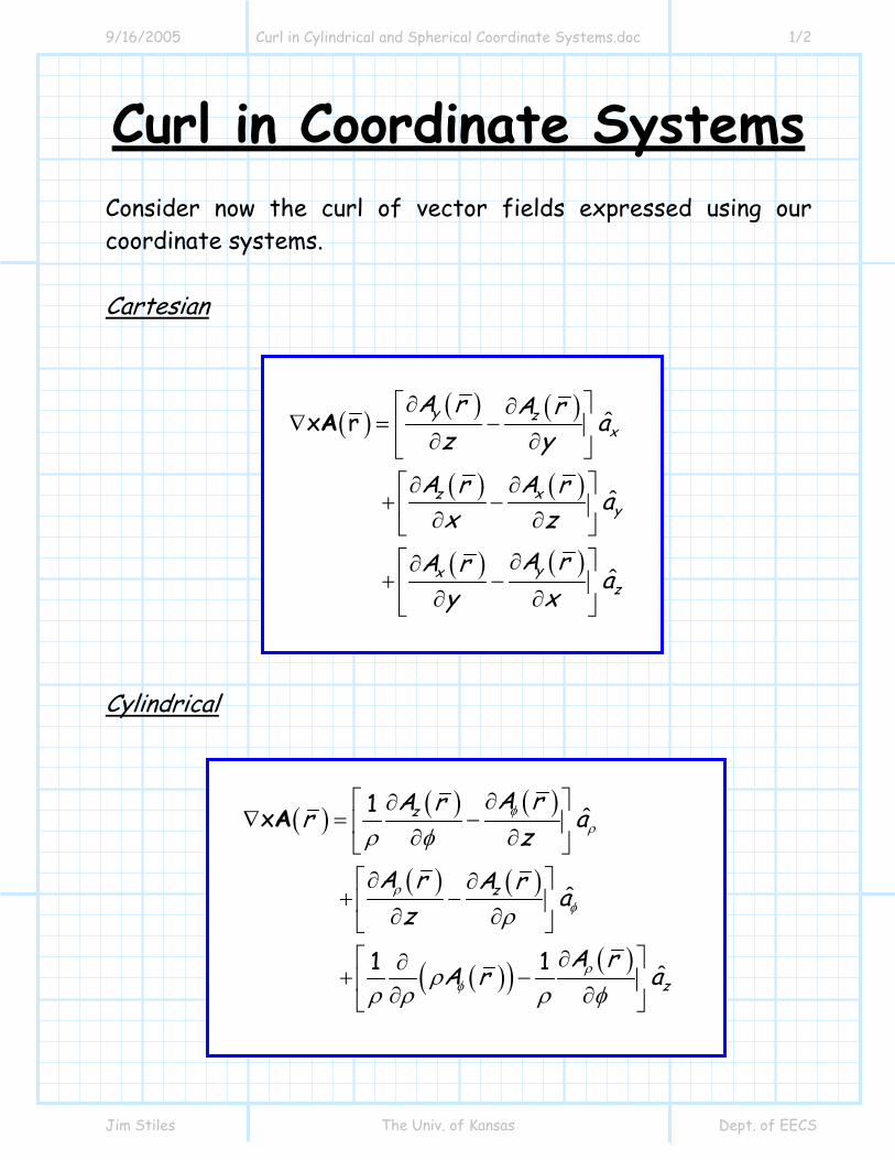
Curl in Coordinate Systems Consider now the curl of vector fields expressed using our coordinate systems. Cartesian

( ) ( ) ( )

( ) ( )

( ) ( )

ˆ

ˆ

ˆ

x r y zx

z xy

yxz

A r A r az y

A r A r ax z

A rA r ay x

∂⎡ ⎤∂∇ = −⎢ ⎥∂ ∂⎣ ⎦

∂ ∂⎡ ⎤+ −⎢ ⎥∂ ∂⎣ ⎦

∂⎡ ⎤∂+ −⎢ ⎥

∂ ∂⎣ ⎦

A

Cylindrical

( ) ( ) ( )

( ) ( )

( )( ) ( )

ˆ

ˆ

ˆ

1x

1 1

z

z

z

A rA rr az

A r A r az

A rA r a

φρ

ρφ

ρφ

ρ φ

ρ

ρρ ρ ρ φ

∂⎡ ⎤∂∇ = −⎢ ⎥∂ ∂⎣ ⎦

∂⎡ ⎤∂+ −⎢ ⎥∂ ∂⎣ ⎦

∂⎡ ⎤∂+ −⎢ ⎥∂ ∂⎣ ⎦

A

9/16/2005 Curl in Cylindrical and Spherical Coordinate Systems.doc 2/2


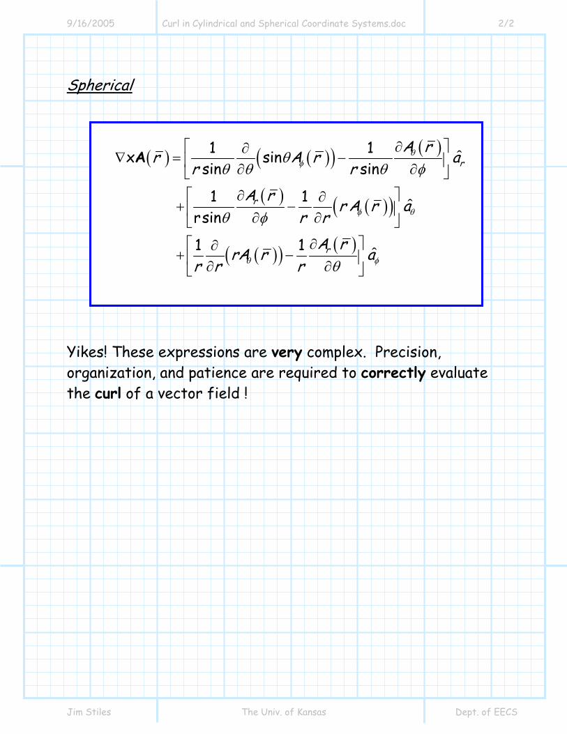
Spherical

( ) ( )( ) ( )

( ) ( )( )

( )( ) ( )

ˆ

ˆ

ˆ

1 1x sinsin sin

1 1rsin

1 1

r

r

r

A rr A r ar r

A r r A r ar r

A rrA r ar r r

θφ

φ θ

θ φ

θθ θ θ φ

θ φ

θ

∂⎡ ⎤∂∇ = −⎢ ⎥∂ ∂⎣ ⎦

∂⎡ ⎤∂+ −⎢ ⎥∂ ∂⎣ ⎦

∂⎡ ⎤∂+ −⎢ ⎥∂ ∂⎣ ⎦

A

Yikes! These expressions are very complex. Precision, organization, and patience are required to correctly evaluate the curl of a vector field !

9/16/2005 Stokes Theorem.doc 1/3


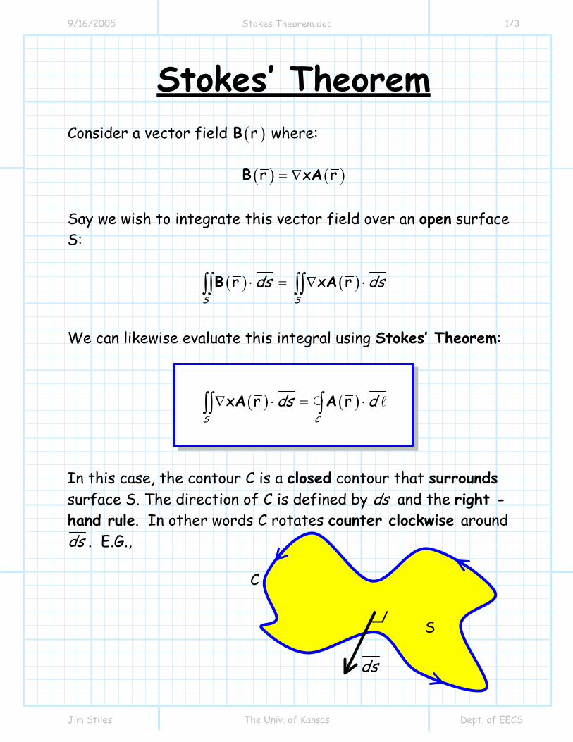
Stokes’ Theorem Consider a vector field ( )rB where:

( ) ( )r x r= ∇B A

Say we wish to integrate this vector field over an open surface S:

( ) ( )r x rS S

ds ds⋅ = ∇ ⋅∫∫ ∫∫B A

We can likewise evaluate this integral using Stokes’ Theorem:

( ) ( )x r rS C

ds d∇ ⋅ = ⋅∫∫ ∫A A

In this case, the contour C is a closed contour that surrounds surface S. The direction of C is defined by ds and the right -hand rule. In other words C rotates counter clockwise around ds . E.G.,

S

C

ds



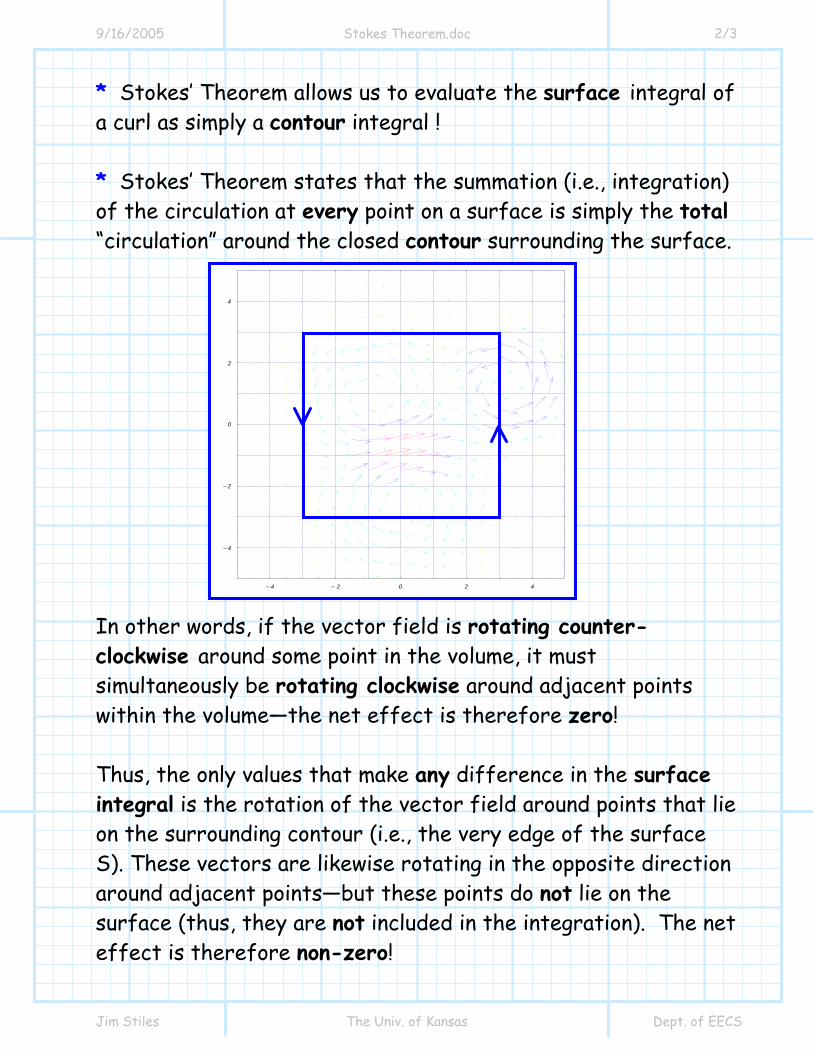
* Stokes’ Theorem allows us to evaluate the surface integral of a curl as simply a contour integral ! * Stokes’ Theorem states that the summation (i.e., integration) of the circulation at every point on a surface is simply the total “circulation” around the closed contour surrounding the surface. In other words, if the vector field is rotating counter-clockwise around some point in the volume, it must simultaneously be rotating clockwise around adjacent points within the volume—the net effect is therefore zero! Thus, the only values that make any difference in the surface integral is the rotation of the vector field around points that lie on the surrounding contour (i.e., the very edge of the surface S). These vectors are likewise rotating in the opposite direction around adjacent points—but these points do not lie on the surface (thus, they are not included in the integration). The net effect is therefore non-zero!

-4 - 2 0 2 4

-4

-2

0

2

4



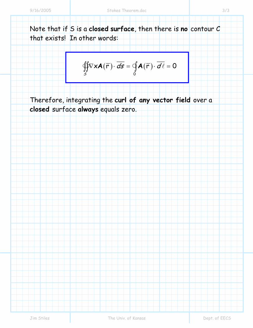
Note that if S is a closed surface, then there is no contour C that exists! In other words:

( ) ( )0

x r r 0S

ds d∇ ⋅ = ⋅ =∫∫ ∫A A

Therefore, integrating the curl of any vector field over a closed surface always equals zero.

9/16/2005 The Curl of a Conservative Field.doc 1/4


The Curl of Conservative Fields

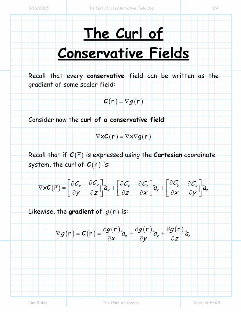
Recall that every conservative field can be written as the gradient of some scalar field:

( ) ( )r rg= ∇C Consider now the curl of a conservative field:

( ) ( )x r x g r∇ = ∇ ∇C

Recall that if ( )rC is expressed using the Cartesian coordinate system, the curl of ( )rC is:

( )x r ˆ ˆ ˆy yz x z xx y z

C CC C C Ca a ay z z x x y

∂ ∂⎡ ⎤ ⎡ ⎤∂ ∂ ∂ ∂⎡ ⎤∇ = − + − + −⎢ ⎥ ⎢ ⎥⎢ ⎥∂ ∂ ∂ ∂ ∂ ∂⎣ ⎦⎣ ⎦ ⎣ ⎦C

Likewise, the gradient of ( )rg is:

( ) ( ) ( ) ( ) ( )r r rr r ˆ ˆ ˆx y zg g gg a a a

x y z∂ ∂ ∂

∇ = = + +∂ ∂ ∂

C



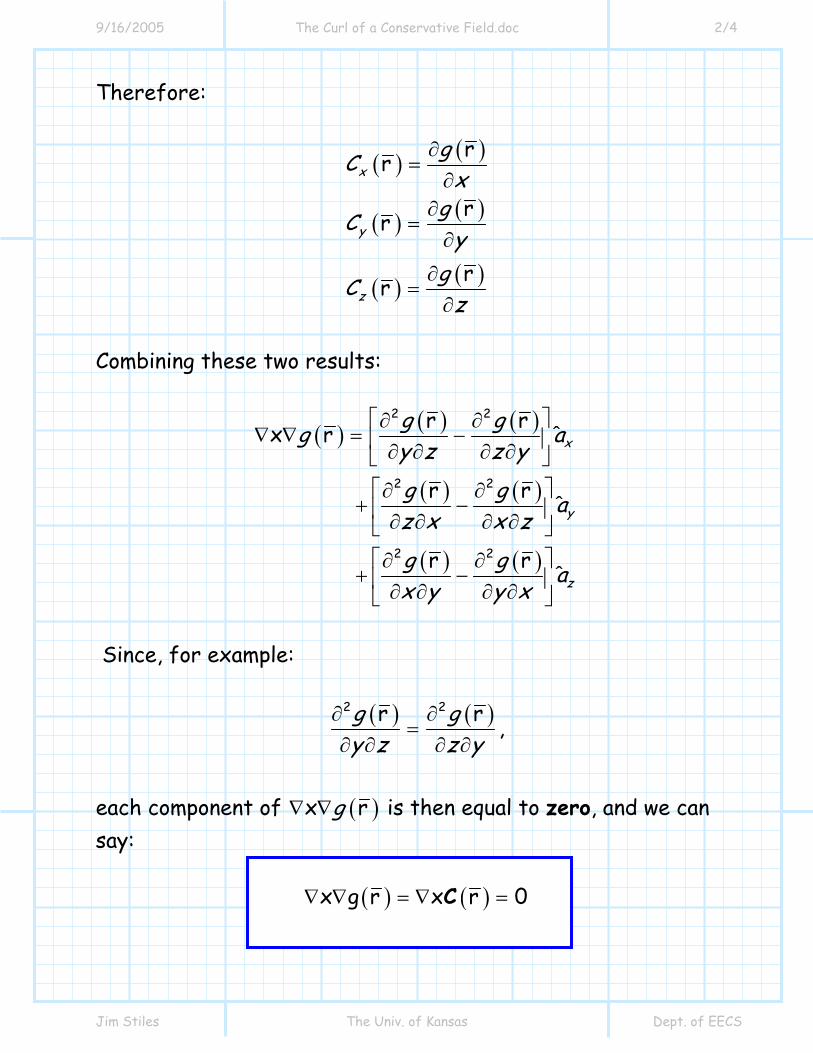
Therefore:

( ) ( )

( ) ( )

( ) ( )

rr

rr

rr

x

y

z

gCx

gCy

gCz

∂=

∂∂

=∂

∂=

∂

Combining these two results:

( ) ( ) ( )

( ) ( )

( ) ( )

2 2

2 2

2 2

r rx r

r r

r r

ˆ

ˆ

ˆ

x

y

z

g gg ay z z yg g az x x zg g ax y y x

⎡ ⎤∂ ∂∇ ∇ = −⎢ ⎥∂ ∂ ∂ ∂⎣ ⎦

⎡ ⎤∂ ∂+ −⎢ ⎥∂ ∂ ∂ ∂⎣ ⎦⎡ ⎤∂ ∂

+ −⎢ ⎥∂ ∂ ∂ ∂⎣ ⎦

Since, for example:

( ) ( )2 2r rg gy z z y

∂ ∂=

∂ ∂ ∂ ∂,

each component of ( )x rg∇ ∇ is then equal to zero, and we can say:

( ) ( )x g r x r 0∇ ∇ = ∇ =C



The curl of every conservative field is equal to zero ! Likewise, we have determined that:

( )x r 0g∇ ∇ =

for all scalar functions ( )g r .

Q: Are there some non-conservative fields whose curl is also equal to zero? A: NO! The curl of a conservative field, and only a conservative field, is equal to zero.

Thus, we have way to test whether some vector field ( )rA is conservative: evaluate its curl!

1. If the result equals zero—the vector field is conservative.

2. If the result is non-zero—the vector field is not

conservative.



Let’s again recap what we’ve learned about conservative fields:

1. The line integral of a conservative field is path

independent. 2. Every conservative field can be expressed as the

gradient of some scalar field. 3. The gradient of any and all scalar fields is a

conservative field. 4. The line integral of a conservative field around any

closed contour is equal to zero. 5. The curl of every conservative field is equal to zero. 6. The curl of a vector field is zero only if it is

conservative.

9/16/2005 The Solenoidal Vector Field.doc 1/4


The Solenoidal Vector Field

1. We of course recall that a conservative vector field ( )rC can be identified from its curl, which is always equal to zero:

( )x r 0∇ =C

Similarly, there is another type of vector field ( )rS , called a solenoidal field, whose divergence is always equal to zero:

( )r 0∇ ⋅ =S

Moreover, we find that only solenoidal vector have zero divergence! Thus, zero divergence is a test for determining if a given vector field is solenoidal. We sometimes refer to a solenoidal field as a divergenceless field. 2. Recall that another characteristic of a conservative vector field is that it can be expressed as the gradient of some scalar field (i.e., ( ) ( )r rg= ∇C ).



Solenoidal vector fields have a similar characteristic! Every solenoidal vector field can be expressed as the curl of some other vector field (say ( )rA ).

( ) ( )r x r= ∇S A Additionally, we find that only solenoidal vector fields can be expressed as the curl of some other vector field. Note this means that:

The curl of any vector field always results in a solenoidal field!

Note if we combine these two previous equations, we get a vector identity:

( )x r 0∇ ⋅∇ =A a result that is always true for any and every vector field ( )rA . Note this result is analogous to the identify derived from conservative fields:

( )x r 0g∇ ∇ =

for all scalar fields ( )rg .



3. Now, let’s recall the divergence theorem:

( ) ( )∇ ⋅ = ⋅∫∫∫ ∫∫V S

dv dsr rA A

If the vector field ( )rA is solenoidal, we can write this theorem as:

( ) ( )r rV S

dv ds∇ ⋅ = ⋅∫∫∫ ∫∫S S

But of course, the divergence of a solenoidal field is zero ( ( )r 0∇ ⋅ =S )! As a result, the left side of the divergence theorem is zero, and we can conclude that:

( )r 0S

ds⋅ =∫∫S

In other words the surface integral of any and every solenoidal vector field across a closed surface is equal to zero. Note this result is analogous to evaluating a line integral of a conservative field over a closed contour

( )r 0C

d⋅ =∫ C



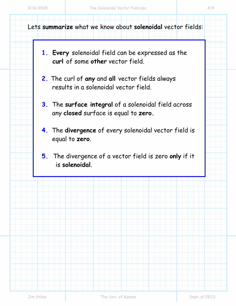
Lets summarize what we know about solenoidal vector fields:

1. Every solenoidal field can be expressed as the curl of some other vector field.

2. The curl of any and all vector fields always

results in a solenoidal vector field. 3. The surface integral of a solenoidal field across

any closed surface is equal to zero.

4. The divergence of every solenoidal vector field is equal to zero.

5. The divergence of a vector field is zero only if it

is solenoidal.

9/16/2005 The Laplacian.doc 1/2


The Laplacian Another differential operator used in electromagnetics is the Laplacian operator. There is both a scalar Laplacian operator, and a vector Laplacian operator. Both operations, however, are expressed in terms of derivative operations that we have already studied ! The Scalar Laplacian The scalar Laplacian is simply the divergence of the gradient of a scalar field:

( )rg∇ ⋅∇

The scalar Laplacian therefore both operates on a scalar field and results in a scalar field. Often, the Laplacian is denoted as “ 2∇ ”, i.e.:

( ) ( )2 r rg g∇ ∇ ⋅ ∇

From the expressions of divergence and gradient, we find that the scalar Laplacian is expressed in Cartesian coordinates as:

( ) ( ) ( ) ( )2 2 22

2 2 2r r rr g g gg

x y z∂ ∂ ∂

∇ = + +∂ ∂ ∂

9/16/2005 The Laplacian.doc 2/2


The scalar Laplacian can likewise be expressed in cylindrical and spherical coordinates; results given on page 53 of your book. The Vector Laplacian The vector Laplacian, denoted as ( )2 r∇ A , both operates on a vector field and results in a vector field, and is defined as:

( ) ( )( ) ( )2 r r x x r∇ ∇ ∇ ⋅ − ∇ ∇A A A

Q: Yikes! Why the heck is this mess referred to as the Laplacian ?!? A: If we evaluate the above expression for a vector expressed in the Cartesian coordinate system, we find that the vector Laplacian is:

( ) ( ) ( ) ( )2 2 2 2r r r rˆ ˆ ˆx x y y z zA a A a A a∇ = ∇ + ∇ + ∇A

In other words, we evaluate the vector Laplacian by evaluating the scalar Laplacian of each Cartesian scalar component! However, expressing the vector Laplacian in the cylindrical or spherical coordinate systems is not so straightforward—use instead the definition shown above!

9/16/2005 Helmholtz Theorems.doc 1/6


Helmholtz’s Theorems Consider a differential equation of the following form:

( ) ( )d f tg tdt

=

where g (t) is an explicit known function, and f (t) is the unknown function that we seek. For example, the differential equation :

2 ( )3 1 d f tt tdt

+ − =

has a solution:

23( )

2tf t t t c= + − +

Thus, the derivative of f (t) provides sufficient knowledge to determine the original function f (t) (to within a constant). An interesting question, therefore, is whether knowledge of the divergence and or curl of a vector field is sufficient to determine the original vector field.



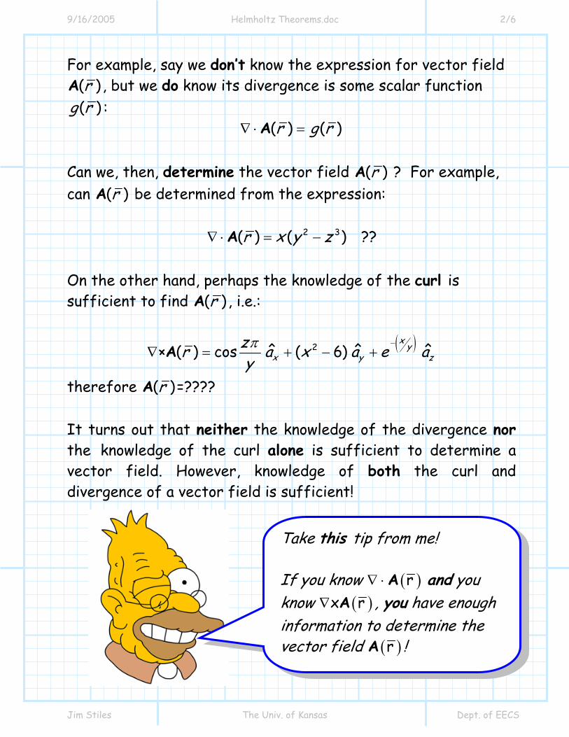
For example, say we don’t know the expression for vector field ( )rA , but we do know its divergence is some scalar function ( )g r :

( ) ( )r g r∇ ⋅ =A

Can we, then, determine the vector field ( )rA ? For example, can ( )rA be determined from the expression:

2 3( ) ( )r x y z∇ ⋅ = −A ??

On the other hand, perhaps the knowledge of the curl is sufficient to find ( )rA , i.e.:

( )2ˆ ˆ ˆ× ( ) cos ( 6)x y

x y zzr a x a e ayπ −

∇ = + − +A

therefore ( )rA =???? It turns out that neither the knowledge of the divergence nor the knowledge of the curl alone is sufficient to determine a vector field. However, knowledge of both the curl and divergence of a vector field is sufficient! Take this tip from me!

If you know ( )r∇ ⋅A and you know ( )x r∇ A , you have enough information to determine the vector field ( )rA !



Q: But why do we need knowledge of both the divergence and curl of a vector field in order to determine the vector field? That’s correct! Any and every possible vector field ( )rA can be expressed as the sum of a conservative field ( ( )rAC ) and a solenoidal field ( ( )rAS ) :

( ) ( ) ( )r r rA A= +A C S

Note then if ( )r 0A =C , the vector field ( ) ( )r rA=A S is solenoidal. Likewise, if ( )r 0A =S the vector field ( ) ( )r rA=A C is conservative.

Of course, if neither term is zero (i.e., ( )r 0A ≠C and

( )r 0A ≠S ), the vector field ( )rA is neither conservative nor solenoidal!

A: I know the answer to that as well! Its because every vector field can be written as the sum of a conservative field and a solenoidal field!



Consider then what happens when we take the divergence of a vector field ( )rA :

( ) ( ) ( )( )( )

r r rr 0r

A A

A

A

∇ ⋅ = ∇ ⋅ + ∇ ⋅

= ∇ ⋅ +

= ∇ ⋅

A C SCC

Look what happened! Since the divergence of a solenoidal field is zero, the divergence of a general vector field ( )rA really just tells us the divergence of its conservative component.

The divergence of a vector field tells us nothing about its solenoidal component ( )rAS !

Thus, from ( )r∇ ⋅A we can determine ( )rAC , but we haven’t a clue about what ( )rAS is! Likewise, the curl of ( )rA is:

( ) ( ) ( )( )

( )

x r x r x r0 x r

x r

A A

A

A

∇ = ∇ + ∇

= + ∇

= ∇

A C SS

S

Look what happened! Since the curl of a conservative field is zero, the curl of a general vector field ( )rA really just tells us the curl of its solenoidal component.

The curl of a vector field tells us nothing about its conservative component ( )rAC !



Thus, from ( )x r∇ A we can determine ( )rAS , but we haven’t a clue about what ( )rAC is!

CONCLUSION: We require knowledge of both ( )r∇ ⋅A (for ( )rAC ) and ( )x r∇ A (for ( )rAS ) to

determine the vector field ( )rA .

From a physical stand point, this makes perfect sense! Recall that we determined the curl ( )x r∇ A identifies the rotational sources of vector field ( )rA , while the divergence

( )r∇ ⋅A identifies the divergent (or convergent) sources. Once we know the sources of vector field ( )rA , we can of course find vector field ( )rA . Q: Exactly how do we find ( )rA from its sources ( ( )r∇ ⋅A and

( )x r∇ A ) ??

A1: I don’t know.



A2: Note the sources of a vector field are determined from derivative operations (i.e., divergence and curl) on the vector field. We can therefore conclude that a vector field ( )rA can be determined from its sources with integral operations!

We’ll learn much more about integrating sources later in the course!

the gradient - ittcjstiles/220/handouts/section_2_5_the_calculus_of... · taking the gradient of...

Documents