signal detection for ofdm and ds-cdma with gradient and ... · signal detection for ofdm and...

Signal Detection for OFDM and DS-CDMA with Gradient and

Blind Source Separation Principles

M. G. S. Sriyananda, J. Joutsensalo, and T. HamalainenDepartment of Mathematical Information Technology,

Faculty of Information Technology,P.O. Box 35, FI-40014 University of Jyvaskyla,

FINLANDEmail: {gamage.m.s.sriyananda, jyrki.j.joutsensalo, timo.t.hamalainen}@jyu.fi

Abstract : -Signal recovery mechanisms for both Orthogonal Frequency Division Multiplexing (OFDM) and DirectSequence - Code Division Multiple Access (DS-CDMA) with the assistance of principles of Blind Source Separation(BSS) and Gradient Algorithms (GAs) are presented. Elimination or reduction of undesirable influences encountered within the wireless interface is targeted using a set of filter coefficients. Four energy functions are used in deriving them. Timecorrelation properties of the channel are used as advantages in introducing the energy functions and they are tried to bejustified followed by a performance evaluation. All the schemes are tested with synchronous downlink system models.Simulations are carried out under slow fading channel conditions with a receiver containing Equal Gain Combining(EGC) and BSS algorithms. It could be noted that, better performance for this predominant air interface communicationtechniques can be achieved with this combined schemes. It is important grasp the fact that, these schemes can be promotedas low complexity simple matrices based processing mechanisms.

Keywords — Blind Source Separation, Gradient Algorithms, OFDM, DS-CDMA, Slow Fading

1 IntroductionDistortion and mixing of signals during a process of airinterface communication is a common scenario. Aboutthree main categories of signal recovery algorithms basedon the availability of prior information about the mixingprocess or the mixture are found in statistical wirelesssignal processing. They are blind, semi-blind and non-blind or normal schemes. Two fundamental properties areemphasized by the adjective “blind”. First is no sourcesignals are observed. Second is no information is availableabout the mixture. The implication of no prior informationis available about the transfer is leaded by this. ThereforeBlind Source or Signal Separation can be introduced as aprocess used for recovery of unobserved signals or sourcesfrom several observed mixtures. In implementations usuallythe observation values are obtained by output of a setof sensors. Sensors are designed such that each receivesa different combination of the source signals. The corestrength of the Blind Source Separation (BSS) model is theweakness or the least dependence on the prior information.That made it a versatile tool for extracting the spatialdiversity provided by an array of sensors. A statisticallystrong plausible assumption of independence between thesource signals is used to compensate the fact of lacking ofprior knowledge about the mixture.

Outcomes of a attempt taken to derive a set of BSSschemes with the aid of gradient algorithm are disclosedin this paper and it is structured as follows. BSS solutionsderived using the gradient principles are unveiled in Section2. Then those solutions are converted to customizedschemes for Orthogonal Frequency Division Multiplexing

(OFDM) and Direct Sequence - Code Division MultipleAccess (DS-CDMA) systems. Two system models forbaseband system simulations are discussed separately inSection 3. In Section 4, system parameters and simulationresults are presented in detail. Finally conclusion is givenin Section 5.

2 BSS Models and GradientAlgorithm

Having more sensors than sources in dealing withnoisy observations, complex signals and mixtures areof much practical importance [1], [2]. Different typesof approaches and solutions that take advantage ofnonstationarity of sources to achieve better performancethan the classical methods can be seen [3], [4]. Expansionand development of basic BSS models and algorithms innumber of directions giving solutions for many complicatedproblems can be seen. They include noisy observationsand complex signals and mixtures. Further they areapplicable to the standard narrow band array processingor beamforming models and convolutive mixtures leadingto multichannel blind deconvolution problems. Some ofthese approaches can only separate stationary non-Gaussiansignals. Due to these limitations, poor performance isobtained when dealing with some real sources, like audiosignals. Biomedical signal analysis and processing (ECG,EEG, MEG) [5], [6], [7] computer vision and imagerecognition, communications signal processing [8] aresome of such most sensitive areas. Some disciplines thatare not directly connected with the basic human needs,

WSEAS TRANSACTIONS on SIGNAL PROCESSING M. G. S. Sriyananda, J. Joutsensalo, T. Hamalainen

E-ISSN: 2224-3488 100 Issue 3, Volume 8, July 2012

http://www.mit.jyu.fi

http://www.jyu.fi

economic or other profitable aspects like geophysical dataprocessing, data mining, acoustics and speech recognitionare being rapidly developed where a significant role canbe played by Blind Source Separation (BSS) principles.Mathematical optimizations based on the principles ofGradient Algorithms (GAs) are widely used in the aresof civil, chemical, mechanical, and aerospace engineering,data networks, finance, supply chain management andmany other areas [9].

It is shown that binary independent component analysis(ICA) can be uniquely identifiable under the disjunctivegeneration model [10]. Same time a deterministic iterativealgorithm to determine the distribution of the latentrandom variables and the mixing matrix is proposed. Theseschemes can easily be applied for scenarios in networkresource management. A generalization of the matchedsubspace filter for the detection of unknown signalsin a background of non-Gaussian and nonindependentnoise is unveiled in [11]. How efficiently the basicBSS theories can be applied in frequency domain isis disclosed in [12]. In this approach, time-domainsignals are transformed into time-frequency series andthe separation is performed by applying ICA at eachfrequency envelope. It can be attempted to customize theseapproaches to any wireless communication system. A semi-blind compensation scheme for both frequency-dependentand frequency independent I/Q imbalance based on ICAin multiple-input multiple-output (MIMO) OFDM systems,where ICA is applied to compensate for I/Q imbalance andequalize the received signal jointly, without any spectraloverhead is given in [13]. This can be recognized as aneffort taken to improve the throughput performance ofOFDM as same as the approach presented in this document.

2.1 General BSS ModelA number of successfully completed research studiestargeting separation of sources on linear instantaneousmixtures can be found. They are with the vital primaryassumption that the sources must be independent [3]. Herealso a simple information symbol transfer process is con-sidered. Source signals are denoted by s(t) with a mixtureof coefficient values A, where A is a F ×B matrix.Element f, b is denoted by af,b. s(t) is modeled with B sig-nal elements as s(t) = [s1(t), s2(t), ..., sb(t), ..., sB(t)]

T ,where sb(t) is the signal element b at time t. Coefficientvalue of s1(t) is a1, a1 = [a1,1, a2,1, ..., af,1, ..., aF,1]

T .Additive independent and identically distributed (IID)white noise and colored noise are indicated byw(t) = [w1(t), w2(t), ..., wf (t), ..., wF (t)]

T and w′(t)respectively. wf (t) is the noise element f at time t.The receive signal matrix for a basic BSS processx(t) = [x1(t), x2(t), ..., xf (t), ..., xF (t)]

T at time t withB unknown input or sources and F output or sensorobservations can be given as [3], [14] and [15],

x(t) = As(t) +w(t) = s1(t)a1 +w′(t) (1)

where s2(t), s3(t), ..., sb(t), ..., sB(t) are independent oruncorrelated symbols or signals. Signal s1(t) is timecorrelated. When appropriately shaped mapped symbolsare considered and the time delay is sufficiently shorterc1 = E {s1(t)s1(t+ τ)} ≈ E

{s21(t)

}. The differential cor-

relation matrix C(τ) at a small time difference τ is given[16] as follows, where matrix transpose is symbolized by·T ,

C(τ) = E{x(t)xT (t+ τ)

}= c1a1a

T1 +Rτ (2)

The ordinary correlation matrix R is,

R = E{x(t)xT (t)

}(3)

= AE{s(t)sT (t)

}AT + σ2I

= c1a1aT1 +R0

Noise variance is given by σ2. It is assumed that‖R0‖ > ‖Rτ‖, where ‖·‖ is Frobenius or 2-norm.

The output y(t) or y of the receiver with coefficient urcis,

y = uTrcx (4)

The output power E{y2(t)

}is derived by (3) and (4) as,

E{y2(t)

}= uTrcRurc (5)

The energy functions J1 (u, λ1), J2 (u, λ2), J3 (u, λ3)and J4 (u, λ4) that are dependent of the measured signalvalues x(t) or x are given in (6), (7), (8) and (9). u isa variable coefficient similar to urc. The differential crosscorrelation matrix C is estimated same as the equation (2).λ1, λ2, λ3 and λ4 are the Lagrangian multipliers. Matrixinverse is referred by ·−1.

J1 (u, λ1) = uTCu+ λ1(I− uTRu

)(6)

J2 (u, λ2) = uTC−1u+ λ2(I− uTRu

)(7)

J3 (u, λ3) = uTCu+ λ3(I− uTR−1u

)(8)

J4 (u, λ4) = uTC−1u+ λ4(I− uTR−1u

)(9)

The signal s1(t)a1 is targeted to be extracted. In eachof the (6) and (8), noise component of w′(t) is tried tobe removed while passing the signal s1(t)a1. In (7) or(9), it is the interference component in w′(t). In (6) or(8), the projection of u to the effective space spanned bythe matrix C is tried to be minimized by the first terms.The output power to the inverse process is minimizedby u respectively where C is produced. In all (6) - (9),time correlated signal portion s1(t)a1 is included withC. Resulting uTCu is expected to be in minimum. It isexpected that the signal s1(t)a1 is passed quite well byu. Minimization of the projection of u to the effectivespaces spanned by R are tried by the second terms ofthe equations. Similarly minimization of the projection ofu to the effective space spanned by C−1 is tried by thefirst terms of the (7) or (9). Here also the output power toinverse method is minimized by u, witch C−1 is produced.Due to the inverse matrix, resulting uTC−1u is kept inminimum. It is expected to pass the signal s1(t)a1 quitewell by u. Minimization of the projections of u to the



effective spaces spanned by R−1 are tried by the secondterms of the equations. In all (6) - (9), E

{y2(t)

}is tried

to be minimized. But with correlation, R0 contains muchthe interference part of R. In this case also the desiredsignal s1(t)a1 is filtered well again by u in the respectiveenergy functions.

In the process of optimization, considering the partialderivatives ∂J1(u,λ1)

∂λ1= 0 of (6), ∂J2(u,λ2)

∂λ2= 0 of (7),

∂J3(u,λ3)∂λ3

= 0 of (8) and ∂J4(u,λ4)∂λ4

= 0 of (9),(I− uTRu

)= 0 (10)(

I− uTRu)= 0 (11)(

I− uTR−1u)= 0 (12)(

I− uTR−1u)= 0 (13)

Since (10) and (11) are in the same form, one common termcan be defined as (14). It is considered as u = u1 and theseparameters are not to be used in (6) or (7). Similarly (12)and (13) are in the same form and one common term canbe defined as (15). It is considered as u = u2 and theseparameters are not to be used in (8) or (9).(

I− uT1 Ru1

)= 0 (14)(

I− uT2 R−1u2

)= 0 (15)

Where u1 and u2 at time t are u1(t) and u2(t) respectively.Using (14), u1(t) is defined in two forms u1,1(t) andu1,2(t) as used in (16) and (18) correspondingly. u0

1,1(t)and u0

1,2(t) are defined based on them. Using (15), u2(t)is defined in two forms as u2,1(t) and u2,2(t) as presentedby (20) and (22). u0

2,1(t) and u02,2(t) are defined based

on them. They are all with similar kinds of approaches asthe gradient algorithm [9]. Parameters given by µβ,γ , β =1,2 and γ = 1,2 can be introduced as the correspondingforgetting factors for them. It is clear that u1,1(t), u1,2(t)and their associated parameters are common for both (6)and (7) while u2,1(t), u2,2(t) and their related parametersare common for both (8) and (9). Matrix complex conjugatetranspose is denoted by ∗.

• Common Coefficient 1

u01,1(t) = u1,1(t) + µ1,1

(I−R (16)

. u1,1(t)u∗1,1(t)

)Cu1,1(t)

u11,1(t) =

u01,1(t)∥∥u01,1(t)

∥∥ (17)


u01,2(t) = u1,2(t) + µ1,2

(I−R (18)

. u1,2(t)u∗1,2(t)

)(C+C∗)u1,2(t)

u11,2(t) =

u01,2(t)∥∥u01,2(t)

∥∥ (19)


u02,1(t) = u2,1(t) + µ2,1

(I−R−1 (20)

. u2,1(t)u∗2,1(t)

)Cu2,1(t)

u12,1(t) =

u02,1(t)∥∥u02,1(t)

∥∥ (21)


u02,2(t) = u2,2(t) + µ2,2

(I−R−1 (22)

. u2,2(t)u∗2,2(t)

)(C+C∗)u2,2(t)

u12,2(t) =

u02,2(t)∥∥u02,2(t)

∥∥ (23)

For the iteration m of any of the solutions in (17), (19),(21) or (23),

umc (t) =um−1c (t)∥∥um−1c (t)

∥∥ (24)

where ·1,1, ·1,2, ·2,1 or ·2,2 is represented by ·c.

2.2 Gradient Algorithm Based BSS forOFDM

Higher rate transmission capability, higher bandwidthefficiency and robustness to multipath fading (includingtolerance to frequency-selective fading) and delays aresome of the key factors that brought Orthogonal FrequencyDivision Multiplexing (OFDM) techniques to the forefrontof the sphere of wireless communication. Here theinvolvement of BSS algorithms and GA based approachesin a process of symbol recognition at a basic OFDMreceiver is tested.

Wireless communication system consisting a N sub-carrier (N -point inverse discrete Fourier transform(IDFT)/discrete Fourier transform (DFT)) OFDM [17], [18]transmitter and a receiver is considered. Frequency re-sponse of the channel state information (CSI) of subcarriern during an OFDM symbol period t is signified by Hn(t).Impulse response of the path l of the channel tap k ofthe multipath frequency-selective Rayleigh fading channelwithin the same duration is symbolized by hk,l(t). Each tapis modeled with L independent paths with exponentiallydecaying delay profiles.

Hn(t) =N−1∑k=0

L−1∑l=0

hk,l(t)e−j 2πkn

N (25)

Transmit symbol and normalized additive white Gaussiannoise (AWGN) of subcarrier n for the period t are repre-sented by dn(t) and vn(t) respectively. σ is the standarddeviation to the additive white Gaussian noise. Then thereceive signal rn(t) on subcarrier n during t can beexpressed as in (26).

rn(t) = Hn(t)dn(t) +

(σ√2vn(t)

)(26)



Considering the characteristics of a slow fading channel itcan be assumed that for a given symbol frame, path gainHn(t) = Hn and hk,l(t) = hk,l.

rn(t) = Hndn(t) +

(σ√2vn(t)

)(27)

The receive signal samples of subcarrier n atthe time period containing the symbol dn(t) canbe expressed as rn(t), rn(t+ τ), ..., rn(t+ (p− 1)τ), ...,rn(t+ (P − 1)τ). Where the P receive signal samplesare taken with small time shifts of τ within each in-formation symbol duration. These samples are equiva-lent to x1(t), x2(t), ..., xf (t), ..., xF (t) in (1). Similar to(27), when symbol sample of dn(t) and AWGN of sam-ple p of rn(t) are indicated by dn(t+ (p− 1)τ) andvn(t+ (p− 1)τ) correspondingly, sample p of receivesignal rn(t) is given as,

rn(t+ (p− 1)τ) = Hndn(t+ (p− 1)τ) (28)

+

(σ√2vn(t+ (p− 1)τ)

)For any symbol sample on subcarrier n within a time dura-tion of a transmit symbol dn(t), dn(t+ (p− 1)τ) = dn(t).

rn(t+ (p− 1)τ) = Hndn(t) (29)

+

(σ√2vn(t+ (p− 1)τ)

)rn(t) and rn(t+ τ) are Q×Q square matrices containingthese samples as elements and (P − 1) = Q2.

rn(t) =

rn(t) . . . . . ....

. . ....

. . . . . . rn(t+ (P − 2)τ)

(30)

rn(t+ τ) =

rn(t+ τ) . . . . . ....

. . ....

. . . . . . rn(t+ (P − 1)τ)

(31)

The differential correlation matrix Cn(τ) at a small timedifference τ and ordinary correlation matrix Rn for sub-carrier n according to (2) and (3) are,

Cn(τ) = E {rn(t)r∗n(t+ τ)} (32)Rn = E {rn(t)r∗n(t)} (33)

As in (16), (18), (20) and (22), matrices u1,1,n(t),u1,2,n(t), u2,1,n(t), u2,2,n(t) and associated matricesu01,1,n(t), u0

1,2,n(t), u02,1,n(t), u0

2,2,n(t) of subcarrier nfor the algorithms can be presented as follows. um1,1,n(t),um1,2,n(t), um2,1,n(t), um2,2,n(t) are the correspondingcoefficient matrices for iterations.

• Common Coefficient 1 for Subcarrier n

u01,1,n(t) = u1,1,n(t) + µ1,1

(I−Rn (34)

. u1,1,n(t)u∗1,1,n(t)

)Cnu1,1,n(t)

um1,1,n(t) =um−11,1,n(t)∥∥um−11,1,n(t)

∥∥ (35)


u01,2,n(t) = u1,2,n(t) + µ1,2

(I−Rn (36)

. u1,2,n(t)u∗1,2,n(t)

). (Cn +C∗n)u1,2,n(t)

um1,2,n(t) =um−11,2,n(t)∥∥um−11,2,n(t)

∥∥ (37)


u02,1,n(t) = u2,1,n(t) + µ2,1

(I−R−1n (38)

. u2,1,n(t)u∗2,1,n(t)

)Cnu2,1,n(t)

um2,1,n(t) =um−12,1,n(t)∥∥um−12,1,n(t)

∥∥ (39)


u02,2,n(t) = u2,2,n(t) + µ2,2

(I−R−1n (40)

. u2,2,n(t)u∗2,2,n(t)

). (Cn +C∗n)u2,2,n(t)

um2,2,n(t) =um−12,2,n(t)∥∥um−12,2,n(t)

∥∥ (41)

For OFDM systems, coefficient matrix umc,n(t) for theiteration m for subcarrier n of any of the solutions givenby um1,1,n(t), u

m1,2,n(t), u

m2,1,n(t) or um2,2,n(t) is stated as

in (42). But umc,n(t) is different according to each scenariopresented in (35), (37), (39) and (41).

umc,n(t) =um−1c,n (t)∥∥um−1c,n (t)

∥∥ (42)

Refined receive signal similar to (4) is,

y′n(t) = um∗c,n(t)rn(t) (43)

Elements of matrix y′n(t) can be defined asy′n(t), y

′n(t+ τ), ..., y′n(t+ (p− 1)τ), ..., y′n(t+ (P − 1)τ)

similar to (27). Signal after Equal Gain Combining (EGC)can be expressed as,

yn(t) =1

Q2

H∗n|Hn|2

P∑p=1

y′n(t+ (p− 1)τ) (44)

The simplified matrix format of the receiver output y(t) ory including EGC with coefficients u is given as,

yOFDM = uTOFDMxOFDM (45)

A diagonal matrix uOFDM of dimensions N ×N is con-sidered. Matrix elements um1 (t),um2 (t), ...,umn (t), ...,umN (t)are on the diagonal. The column matrix xOFDM wherethe element n can be given by,

xn(t+ (p− 1)τ) =H∗n|Hn|2

rn(t+ (p− 1)τ) (46)



2.3 Gradient Algorithm based BSS forDS-CDMA

Addition of interference has been recognized as one ofthe main limiting factors for the capacity of the mostCDMA techniques. Basically this interference is generatedfrom the other users in the system and from the externalsources radiating in the same frequency band. Even if itis unlikely to control these types of interferences presentin the environment efficiently, BSS algorithms can bedeveloped to approach these scenarios.

Basic synchronous downlink DS-CDMA [18], [19] isconsidered. Channel impulse response for the path l of thechannel tap of the multipath Rayleigh fading channel attime t is given by Al(t). Each tap is with L independentpaths with exponentially decaying delay profiles.

A(t) =L−1∑l=0

Al(t) (47)

The receive signal rj(t) at time t before despreadingconsisting K simultaneous users, can be expressed as in(48). Time t corresponds to the spreading code element jof each user.

rj(t) =

K∑k=1

A(t)ck,j(t)dk(t) +

(σ√2n(t)

)(48)

Since slow fading is considered it can be assumed that fora given symbol frame path gain A(t) = A.

rj(t) = AK∑k=1

ck,j(t)dk(t) +

(σ√2n(t)

)(49)

where ck,j(t), dk(t) and n(t) are spreading code elementj of the user k at time t, transmit symbols of the user kat time t and normalized additive white Gaussian noiseat time t respectively. σ is the standard deviation to theadditive white Gaussian noise.

Signals at the receiver are sampled P times in smalltime shifts of τ within each spreading code elementtime duration where samples for ck,j(t) can be given asrj(t), rj(t+ τ), ..., rj(t+ (p− 1)τ), ..., rj(t+ (P − 1)τ).They are equivalent to x1(t), x2(t), ..., xf (t), ..., xF (t)in (1). Samples p of spreading code element sampleck,j(t), symbol dk(t) and additive white Gaussian noiseare indicated by ck,j(t+ (p− 1)τ), dk(t+ (p− 1)τ) andn(t+ (p− 1)τ) correspondingly. Sample p of receive sig-nal rj(t) can be given as similar to (49),

rj(t+ (p− 1)τ) = AK∑k=1

ck,j(t+ (p− 1)τ) (50)

. dk(t+ (p− 1)τ)

+

(σ√2n(t+ (p− 1)τ)

)

In a time duration of a spreading code element,for any sample ck,j(t+ (p− 1)τ) = ck,j(t) anddk(t+ (p− 1)τ) = dk(t).

rj(t+ (p− 1)τ) = AK∑k=1

ck,j(t)dk(t) (51)

+

(σ√2n(t+ (p− 1)τ)

)rj(t) and rj(t+ τ) are Q×Q square matrices containingthese samples as elements and (P − 1) = Q2 .

rj(t) =

rj(t) . . . . . ....

. . ....

. . . . . . rj(t+ (P − 2)τ)

(52)

rj(t+ τ) =

rj(t+ τ) . . . . . ....

. . ....

. . . . . . rj(t+ (P − 1)τ)

(53)

From (2) and (3),

C(τ) = E{rj(t)r

∗j (t+ τ)

}(54)

R = E{rj(t)r

∗j (t)

}(55)

For the DS-CDMA systems coefficients for thealgorithms can be introduced using (16) and (18).With mapping um1,1(t) and um1,2(t) to hm1 (t) and hm2 (t)respectively,


h01(t) = h1(t) + µ1,1(I−Rh1(t)h

∗1(t)) (56)

. Ch1(t)

hm1 (t) =hm−11 (t)∥∥hm−11 (t)

∥∥ (57)


hm2 (t) = h2(t) + µ1,2(I−Rh2(t)h∗2(t)) (58)

. (C+C∗)h2(t)

hm2 (t) =hm−12 (t)∥∥hm−12 (t)

∥∥ (59)

For the iteration m of any of the solutions given forDS-CDMA is the same as (24) for the any of the solutionsgiven by hm1 (t) or hm2 (t). But here also hmc (t) is differentaccording to the scenario.

hmc (t) =hm−1c (t)∥∥hm−1c (t)

∥∥ (60)

Refined receive signal similar to (4) is,

y′j(t) = hm∗c,j (t)rj(t) (61)

Elements of matrix y′j(t) can be defined asy′j(t), y

′j(t+ τ), ..., y′j(t+ (p− 1)τ), ..., y′j(t+ (P − 1)τ)

similar to (49). Signal after EGC that is used fordespreading can be expressed as,

yj(t) =1

Q2

A∗

|A|2P∑p=1

y′j(t+ (p− 1)τ) (62)



3 System ModelsTwo system models for OFDM and DS-CDMA areseparately considered under the same conditions. Adownlink frequency-selective slow fading Rayleigh channelis used as the air interface. It is assumed that perfect pathgain values are available at the receivers and transmitreceiver setups are properly synchronized under all theconditions. EGC, one of the most stable combiningtechnique is used to treat CSIs.

3.1 OFDM System ModelElementary system model used for discrete time base bandsimulations is given in Figure 1. The single transmitand single receive antenna setup is equipped with anOFDM transmitter and a receiver [17], [18]. Receiver issupplemented with lesser complex iterative BSS algorithmswith multiple sampling for each receive symbol on eachsubcarrier. Same system model without multiple samplingis used in order to test and verify the results of standardOFDM system [17], [18].

3.2 CDMA System ModelThe DS-CDMA discrete time base band simulation systemmodel in Figure 2 is consist of a transmitter [19] [18] whichcan handle K users using Walsh-Hadamard spreadingsequences [19]. At the receiver, multiple samples foreach receive spread code element are taken. Then iterativelesser complex Gradient principles based BSS algorithmsfollowed by EGC are employed. Same system model withno multiple sampling mechanism for receive spread codeelements is used in order to test and verify the resultscomparing with a standard downlink synchronous DS-CDMA system [19], [18].

4 System Parameters and SimulationResults

System parameters and simulation results for the bothcategories of techniques are separately presented. Simula-tions are carried out for non optimized forgetting factorwith value -0.01. Each channel tap is modeled with 4independent paths and it is assumed that there is novariation of the signal within symbol duration due to anyother reason. Since the system is operated under slowfading conditions the assumption becomes much stronger.

4.1 OFDM SystemsStandard or basic 64, 32 and 16 subcarrier OFDMtransmitter receiver arrangements with a binary informationbit generator and binary phase shift keying (BPSK) symbolmapping are used for the simulations. After interleaving,

symbols are serial to parallel converted among subcarriersand sent through the slow Rayleigh fading channel.Multiple signal samples are taken from each receive symbolon every subcarrier for the purpose of using GA based BSSschemes. By considering the characteristics of the channel[20] and time correlation properties of the binary waveforms [16], samples are taken only within the first 20% oftime duration of an information symbol. Systems with theBSS schemes are configured to be operated a number ofiterations.

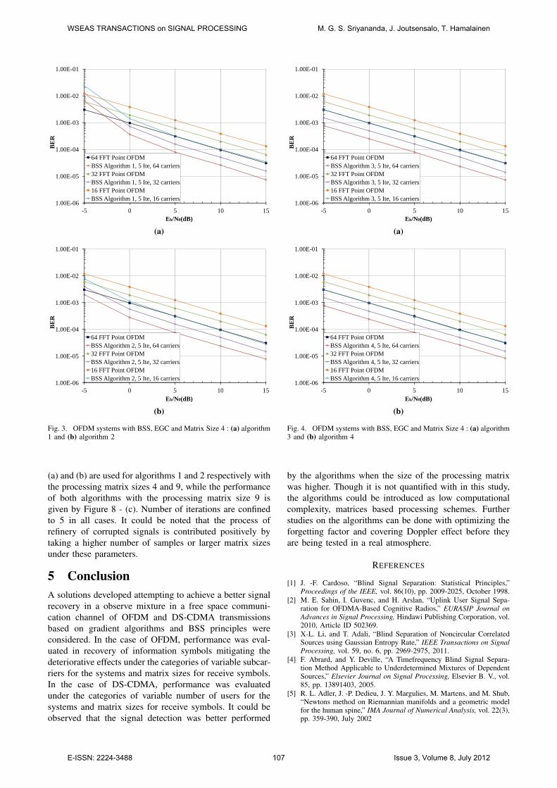
In the case of first set of simulations, variable number ofsubcarriers for the BSS scheme is considered. Performanceresults for 16, 32 and 64 subcarriers are obtained for thisclassification with processing matrix size 4 (5 receive signalsamples) for each of the receive symbol on every subcarrier.Rest of the parameters and conditions of the model aremaintained as the same. Outcome of the operations ofthe systems namely the OFDM system with the BSSalgorithms and the standard OFDM system is presented inFigures 3 and 4. The results of the schemes 1 (coefficientum1,1,n(t) in (35)) and 2 (coefficient um1,2,n(t) in (37)),worked out for 16, 32 and 64 subcarriers are given byFigure 3 - (a) and (b) separately. In this case the algorithmsbased OFDM systems are competent of outperforming thecorresponding standard OFDM systems. It is importantto notice that the performance of the algorithms arebetter when the signal to noise ratio (SNR) is higher andperformance of the standard systems are comparativelybetter for the lower SNR values. Similarly the resultsof the schemes 3 (coefficient um2,1,n(t) in (39)) and 4(coefficient um2,2,n(t) in (41)) worked out for 16, 32 and 64subcarriers are given by Figure 4 - (a) and (b) respectively.In these cases also, the algorithms based OFDM systemsare capable of outperforming the corresponding standardOFDM systems in respective subcarriers scenarios. Inall occasions, performance is better when the number ofsubcarriers are increased.

Corroborative simulations conducted using the explainedOFDM substructure with the BSS algorithm with differentprocessing matrix sizes and the standard OFDM system areshown in Figure 5 and 6. Other parameters and conditionsare maintained as the same. Performance is scrutinizedfor the BSS schemes 1 (coefficient um1,1,n(t) in (35)) and2 (coefficient um1,2,n(t) in (37)) carried out for processingmatrix sizes 4 and 9 and presented in Figure 5 - (a) and (b)respectively. Outcome of the both algorithms with matrixsize 9 (10 samples) is shown in Figure 5 - (c) where thesimulation curves of the two schemes fall in the vicinityof each other for higher SNR values while showing a cleardifference for lower SNR values. Better bit error rates aredemonstrated by the curves taken for a higher processingmatrix size. Hence it could be resolved that a constructivecontribution is done by a larger processing matrix forthe process of refinery of corrupted symbols under theseparameters. Same way, outcomes of the simulations carriedout for the BSS schemes 3 (coefficient um2,1,n(t) in (39))



( )thk 1,

( )thk 2,

M

( )th lk ,

( )th Lk , Tx OFDM Interleaver

Random Data Generator

Delay Comparison

BER Output

Radio Channel

Rx OFDM, BSS

AWGN Deinterleaver

Transmitter Receiver

Fig. 1. Block diagram of the lowpass equivalent OFDM system model

Fading Channel Tx DS-CDMA

Rx DS–CDMA BSS, MUD

Comparison

Delay

Transmitter

Mobile Radio Channel

Receiver BER Output

AWGN

user-K-1




user-1 user-0

Interleaver

Interleaver

Deinterleaver

Drinterleaver Deinterleaver

Fig. 2. Block diagram of the lowpass equivalent DS-CDMA system model

and 4 (coefficient um2,2,n(t) in (41)) with processing matrixsizes 4 and 9 and presented in Figure 6 - (a) and (b)respectively. Results of the both algorithms with matrixsize 9 is shown in 6 - (c) where the simulation curves ofthe two schemes fall in the vicinity of each other. Betterbit error rates are demonstrated by the curves of takenfor a higher processing matrix sizes. Hence it could beobserved that a constructive contribution is done by alarger processing matrices for the process of detection ofcorrupted information symbols under these parameters.

4.2 DS-CDMA SystemsSystems consisting 16-users with a 16 Walsh-Hadamardcode matrices [19] are considered for simulations. Binaryinformation bit streams of each user are converted tobinary phase shift keying (BPSK) symbols, interleaved andtransmitted through slow fading channel. Multiple signalsamples are obtained corresponding to each of the receivespread code element for the purpose of using the GradientAlgorithm based BSS schemes. Considering the propertiesof the channel [20] and time correlation properties of thebinary wave forms [16] it is decided to take samples only

within the first 20% of time duration of a spread sequenceelement. Systems with the BSS schemes are configured tobe operated for number of iterations.

Performance of the DS-CDMA systems viz. systemwith two BSS algorithms and standard DS-CDMA systemfor different number of users are shown in Figure 7. Allthe other parameters and conditions are maintained as thesame. The results obtained with the both BSS schemescarried out for 2, 4, 8 and 16 users with 5 iterations arepresented in Figure 7 - (a) and (b) respectively. Curves ofthe 2, 4, 8 and 16 users scenarios fall vicinity of each otheras usual. Each receive spread code element is sampled 5times at the receiver creating processing matrix size 4.Here the standard DS-CDMA system is outperformed bythe these algorithms.

Similarly another set of simulation results are obtainedwith different processing matrix sizes for the BSS schemeand each receive spread code element comparing withthe standard DS-CDMA system as indicate by Figure 8.In this development all these algorithms are capable ofoutperforming the standard DS-CDMA system. Figure 8 -



1.00E-03

1.00E-02

1.00E-01

BE

R

1.00E-06

1.00E-05

1.00E-04

-5 0 5 10 15

BE

R

64 FFT Point OFDMBSS Algorithm 1, 5 Ite, 64 carriers32 FFT Point OFDMBSS Algorithm 1, 5 Ite, 32 carriers16 FFT Point OFDMBSS Algorithm 1, 5 Ite, 16 carriers

-5 0 5 10 15Eb/N0(dB)

(a)

1.00E-03

1.00E-02

1.00E-01

BE

R

1.00E-06

1.00E-05

1.00E-04

-5 0 5 10 15

BE

R


-5 0 5 10 15Eb/N0(dB)

(b)

Fig. 3. OFDM systems with BSS, EGC and Matrix Size 4 : (a) algorithm1 and (b) algorithm 2

1.00E-03

1.00E-02

1.00E-01

BE

R

1.00E-06

1.00E-05

1.00E-04

-5 0 5 10 15

BE

R


-5 0 5 10 15Eb/N0(dB)

(a)

1.00E-03

1.00E-02

1.00E-01

BE

R

1.00E-06

1.00E-05

1.00E-04

-5 0 5 10 15

BE

R


-5 0 5 10 15Eb/N0(dB)

(b)

Fig. 4. OFDM systems with BSS, EGC and Matrix Size 4 : (a) algorithm3 and (b) algorithm 4

(a) and (b) are used for algorithms 1 and 2 respectively withthe processing matrix sizes 4 and 9, while the performanceof both algorithms with the processing matrix size 9 isgiven by Figure 8 - (c). Number of iterations are confinedto 5 in all cases. It could be noted that the process ofrefinery of corrupted signals is contributed positively bytaking a higher number of samples or larger matrix sizesunder these parameters.

5 ConclusionA solutions developed attempting to achieve a better signalrecovery in a observe mixture in a free space communi-cation channel of OFDM and DS-CDMA transmissionsbased on gradient algorithms and BSS principles wereconsidered. In the case of OFDM, performance was eval-uated in recovery of information symbols mitigating thedeteriorative effects under the categories of variable subcar-riers for the systems and matrix sizes for receive symbols.In the case of DS-CDMA, performance was evaluatedunder the categories of variable number of users for thesystems and matrix sizes for receive symbols. It could beobserved that the signal detection was better performed

by the algorithms when the size of the processing matrixwas higher. Though it is not quantified with in this study,the algorithms could be introduced as low computationalcomplexity, matrices based processing schemes. Furtherstudies on the algorithms can be done with optimizing theforgetting factor and covering Doppler effect before theyare being tested in a real atmosphere.

REFERENCES

[1] J. -F. Cardoso, “Blind Signal Separation: Statistical Principles,”Proceedings of the IEEE, vol. 86(10), pp. 2009-2025, October 1998.

[2] M. E. Sahin, I. Guvenc, and H. Arslan, “Uplink User Signal Sepa-ration for OFDMA-Based Cognitive Radios,” EURASIP Journal onAdvances in Signal Processing, Hindawi Publishing Corporation, vol.2010, Article ID 502369.

[3] X-L. Li, and T. Adali, “Blind Separation of Noncircular CorrelatedSources using Gaussian Entropy Rate,” IEEE Transactions on SignalProcessing, vol. 59, no. 6, pp. 2969-2975, 2011.

[4] F. Abrard, and Y. Deville, “A Timefrequency Blind Signal Separa-tion Method Applicable to Underdetermined Mixtures of DependentSources,” Elsevier Journal on Signal Processing, Elsevier B. V., vol.85, pp. 13891403, 2005.

[5] R. L. Adler, J. -P. Dedieu, J. Y. Margulies, M. Martens, and M. Shub,“Newtons method on Riemannian manifolds and a geometric modelfor the human spine,” IMA Journal of Numerical Analysis, vol. 22(3),pp. 359-390, July 2002



[6] A. K. Barros, R. Vigario, V. Jousmaki, and N. Ohnishi, “Extractionof Event-related Signals from Multichannel Bioelectrical Measure-ments,” IEEE Transaction on Biomedical Engineering, vol. 47, no.5, pp. 583-588, May 2000.

[7] N. Mammone, F. La Foresta, and F. C. Morabito, “Automatic ArtifactRejection From Multichannel Scalp EEG by Wavelet ICA,” IEEESensors Journal, vol. 12, no. 3, pp. 533-542, March 2012.

[8] M. E. Waheed, “Blind Signal Separation using an Adaptive WeibullDistribution,” International Journal of Physical Sciences, vol. 4(5),pp. 265-270, May 2009.

[9] S. Boyd, and L. Vandenberghe, Convex Optimization. CambridgeUniversity Press. 2004.

[10] H. Nguyen, and R. Zheng, “Binary Independent Component Anal-ysis With or Mixtures,” IEEE Sensors Journal, vol. 59, no. 7, pp.3168-3181, July 2011.

[11] J. Moragues, L. Vergara, and J. Gosalbez, “Generalized MatchedSubspace Filter for Nonindependent Noise Based on ICA,” IEEETransactions on Signal Processing, vol. 59, no. 7, pp. 3430-3434,July 2011.

[12] F. Nesta, P. Svaizer, and M. Omologo, “Convolutive BSS of ShortMixtures by ICA Recursively Regularized Across Frequencies,” IEEETransactions on Audio, Speech, and Language Processing, vol. 19,no. 3, pp. 624-639, March 2011.

[13] J. Gao, X. Zhu, H. Lin, and A. K. Nandi, “Independent ComponentAnalysis Based Semi-blind I/Q Imbalance Compensation for MIMOOFDM Systems,” IEEE Transactions on Wireless Communications,vol. 9, no. 3, pp. 914-920, March 2010.

[14] A. Belouchrani, K. Abed-Meraim, J.-F. Cardoso, and E. Moulines,“A Blind Source Separation Technique using Second-Order Statis-tics,” IEEE Transactions on Signal Processing, vol. 45, no. 2, pp.434-444, February 1997.

[15] L. Parra, and P. Sajda, “Blind Source Separation via GeneralizedEigenvalue Decomposition,” The Journal of Machine Learning Re-search, vol. 4, pp. 1261-1269, December 2003.

[16] S. Haykin, Communication Systems. John Wiley & Sons, Inc. 4thEdition, 2001.

[17] C. K. Sung, and I. Lee, “Multiuser Bit-Interleaved Coded OFDMwith Limited Feedback Information,” IEEE Vehicular TechnologyConference, Dallas, Texas, USA, September 2005.

[18] L. Hanzo, L -L. Yang, E -L. Kuan, and K. Yen, Single- and Multi-Carrier DSCDMA: Multi-User Detection, Space-Time Spreading,Synchronisation, Networking and Standards. John Wiley & Sons, Inc.2003.

[19] S. Verdu, Multiuser Detection. Cambridge University Press, Cam-bridge, U.K. 1998.

[20] J. G. Proakis, Digital Communications. McGraw-Hill, Inc. 4thEdition, 2001.



1.00E-04

1.00E-03

1.00E-02

BE

R

1.00E-06

1.00E-05

1.00E-04

-5 0 5 10 15

BE

R

64 FFT Point OFDMBSS Algorithm 1, 2 Ite, Matrix Size 9BSS Algorithm 1, 2 Ite, Matrix Size 4

-5 0 5 10 15Eb/N0(dB)

(a)

1.00E-04

1.00E-03

1.00E-02

BE

R

1.00E-06

1.00E-05

1.00E-04

-5 0 5 10 15

BE

R


-5 0 5 10 15Eb/N0(dB)

(b)

1.00E-04

1.00E-03

1.00E-02

BE

R

1.00E-06

1.00E-05

1.00E-04

-5 0 5 10 15

BE

R


-5 0 5 10 15Eb/N0(dB)

(c)

Fig. 5. OFDM systems with BSS and EGC : (a) algorithm 1, (b)algorithm 2 and (c) two algorithms with matrix size 9

1.00E-04

1.00E-03

1.00E-02

BE

R

1.00E-06

1.00E-05

1.00E-04

-5 0 5 10 15

BE

R


-5 0 5 10 15Eb/N0(dB)

(a)

1.00E-04

1.00E-03

1.00E-02B

ER

1.00E-06

1.00E-05

1.00E-04

-5 0 5 10 15

BE

R


-5 0 5 10 15Eb/N0(dB)

(b)

1.00E-04

1.00E-03

1.00E-02

BE

R

1.00E-06

1.00E-05

1.00E-04

-5 0 5 10 15

BE

R


-5 0 5 10 15Eb/N0(dB)

(c)

Fig. 6. OFDM systems with BSS and EGC : (a) algorithm 3, (b)algorithm 4 and (c) two algorithms with matrix size 9



1.00E-03

1.00E-02

1.00E-01

BE

R

1.00E-05

1.00E-04

1.00E-03

BE

R

16-user DS-CDMABSS Algorithm 1, 5 Ite, 16 usersBSS Algorithm 1, 5 Ite, 8 usersBSS Algorithm 1, 5 Ite, 4 usersBSS Algorithm 1, 5 Ite, 2 users

-5 0 5 10 15Eb/N0(dB)

(a)

1.00E-03

1.00E-02

1.00E-01

BE

R

1.00E-05

1.00E-04

1.00E-03

BE

R

16-user DS-CDMABSS Algorithm 2, 5 Ite, 16 usersBSS Algorithm 2, 5 Ite, 8 usersBSS Algorithm 2, 5 Ite, 4 usersBSS Algorithm 2, 5 Ite, 2 users

-5 0 5 10 15Eb/N0(dB)

(b)

Fig. 7. 32-user DS-CDMA systems with BSS and EGC : (a) algorithm1 and (b) algorithm 2

1.00E-03

1.00E-02

1.00E-01

BE

R

1.00E-05

1.00E-04

1.00E-03

BE

R

16-user DS-CDMABSS Algorithm 1, 5 Ite, Matrix Size 9BSS Algorithm 1, 5 Ite, Matrix Size 4

-5 0 5 10 15Eb/N0(dB)

(a)

1.00E-03

1.00E-02

1.00E-01B

ER

1.00E-05

1.00E-04

1.00E-03

BE

R


-5 0 5 10 15Eb/N0(dB)

(b)

1.00E-03

1.00E-02

1.00E-01

BE

R

1.00E-05

1.00E-04

1.00E-03

BE

R


-5 0 5 10 15Eb/N0(dB)

(c)

Fig. 8. 32-user DS-CDMA systems with BSS and EGC : (a) algorithm1, (b) algorithm 2 and (c) two algorithms with matrix size 9



signal detection for ofdm and ds-cdma with gradient and ... · signal detection for ofdm and...

Documents