the gpm microwave imager and combined precipitaon algorithms

8th Workshop of International Precipitation Working Group 5thInterna*onalWorkshoponSpace-basedsnowfallMeasurements

3-7 October 2016 Bologna, I

TheGPMMicrowaveImagerandcombinedprecipita7on

algorithms

Christian Kummerow Colorado State University

8th IPWG and 5th IWSSM Joint Workshop Bologna, 3-7 October, 2016

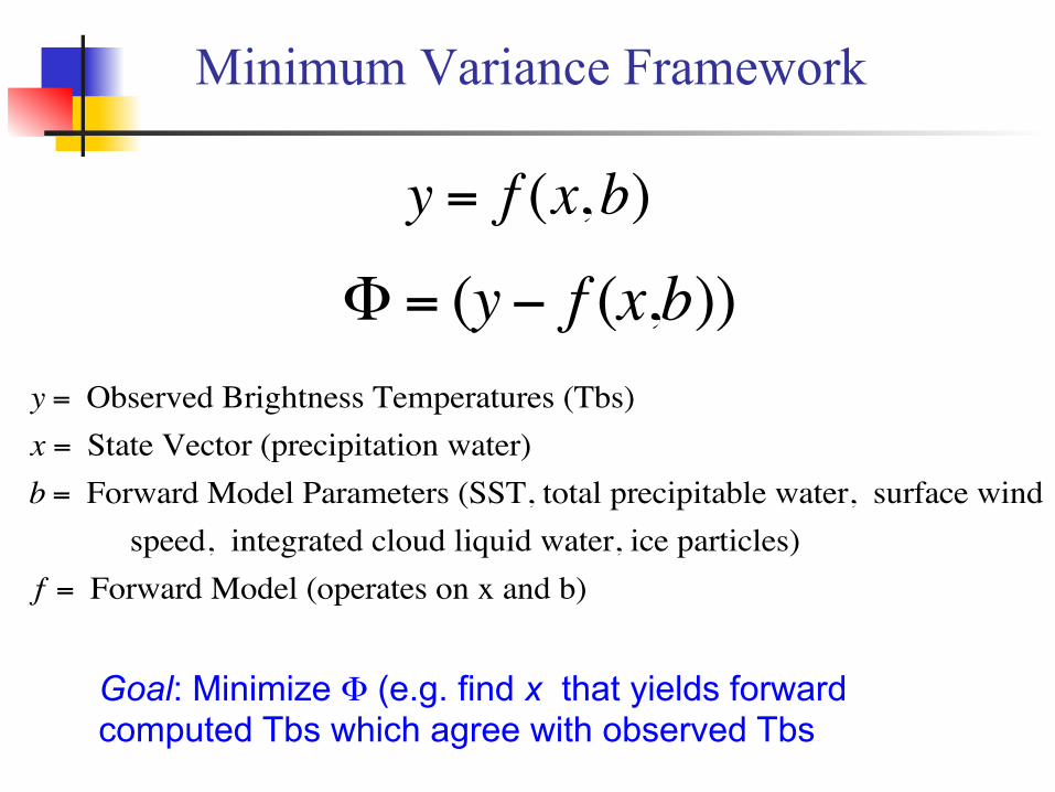
Minimum Variance Framework

y = f (x,b)

y = Observed Brightness Temperatures (Tbs)x = State Vector (precipitation water)b = Forward Model Parameters (SST, total precipitable water, surface wind speed, integrated cloud liquid water, ice particles)f = Forward Model (operates on x and b)

Goal: Minimize Φ (e.g. find x that yields forward computed Tbs which agree with observed Tbs

Φ = (y− f (x,b))

Minimum Variance Framework

2 equations with 2 unknowns

easy

2 barely independent equations with 2 unknowns

hard

Optimal Estimation Framework

€

y = f (x,b) + εb + εyy = Observed Brightness Temperatures (TBs)εb, εy = Error Term (model parameter, measurement error)x = State Vector (total precipitable water, TPW; surface wind speed, WIND; integrated cloud liquid water, LWP)b = Forward Model Parameters (i.e. Scale Height, Lapse Rate, SST)f = Forward Model (operates on x and b); usually the radiative transfer model

Goal: Find that yields forward computed TBs which agree with observed TBs within allotted error range

€

x

Minimize cost function:

€

Φ = (y − f (x,b))T SY−1(y − f (x,b))

TERM 1 + (x − xA )

T SA−1(x − xA )

TERM 2

€

SY = Errors in Measurements and Model

Minimize Differences between Observed and Simulated TBs

Minimize Differences between a priori and retrieved states

€

SA = Errors in xa

€

y = f (x,b) + εb + εy

Optimal Estimation Framework

E(Rj ) =RiJi

i∑

Jii∑

, i =1,n

E(Δw2 ) =

[Rj −E(Rj )]2 J j

j∑

J jj∑

, j =1,n

Ji = exp −12tbo − tb(Ri )⎡⎣ ⎤⎦

TSy +SA( )

−1tbo − tb(Ri )⎡⎣ ⎤⎦

⎧⎨⎩

⎫⎬⎭

Bayesian Retrieval Retrieval

Simplified Bayesian retrieval with assumption that pdf’s of both hydrometeor profiles and observations are realistic and representative:

Expected value Of hydrometeor profile Expected value of errors Cost-function

Observed Simulated Observation & TB-vector TB-vector modelling error

covariance matrix

P(R |Tb )∝P(R)×P(Tb |R)


yi yobs yobs ; σnoise

TheGPMradiometeralgorithm

~ 10 km

TB observed

TB model #1

TB model #2

TB model #3~10 km

TB observed

TB database profile #1



Step1:UseTRMM/GPMSatellitetoderivesetof“Observed”profilesthatdefineana-prioridatabaseofpossiblerainstructures.

Step2:CompareobservedTbtoDatabaseTb.Selectandaveragematchingpairs

Ji = exp −12tbo − tb(Ri )"# $%

TO+S( )−1 tbo − tb(Ri )"# $%

&'(

)*+

GPROF 2010 w. observed database

South Africa

GPROF 2010 w. observed database

GMI Rainfall w. observed database

E(Rj ) =RiJi

i∑

Jii∑

, i =1,n

E(Δw2 ) =

[Rj −E(Rj )]2 J j

j∑

J jj∑

, j =1,n

Ji = exp −12tbo − tb(Ri )⎡⎣ ⎤⎦

TSy +SA( )

−1tbo − tb(Ri )⎡⎣ ⎤⎦

⎧⎨⎩

⎫⎬⎭

Bayesian Retrieval Retrieval

Expected value Of hydrometeor profile Expected value of errors Cost-function

Observed Simulated Observation & TB-vector TB-vector modelling error

covariance matrix



The Bayesian formulation favors results of profiles that occur often in nature. But rare meteorological conditions can also be penalized.

GPROF 2014 Evolution

For Operational Algorithm:

Try not to mix different surface types Try not to mix different environmental conditions

Cloud Profiles Partitioned by TPW

GPROF 2014 Unified Algorithm Structure

PreProcessor (sensor specific)

Standard input file

Spacecraft position Pixel Location, Tbs Pixel Time, EIA Chan Freqs & Errors

GPROFPrecipita*onAlgorithm

L1C Sensor Data Surface&EmissivityClassesECMWF/GANALT2m,TPWAutosnowSnowCoverReynoldsSea-Ice

Ancillary Info / Datasets

SensorProfileDatabase

Complete HDF5 Output file

Post-processor(BinarytoHDF5)

A-PrioriMatchedProfiles-GMI/DPR

JMAforecast-NRTGANAL-Standard

ECMWF-Climatology

Model Preparation

DenotesProcessesrunningattheSIPS

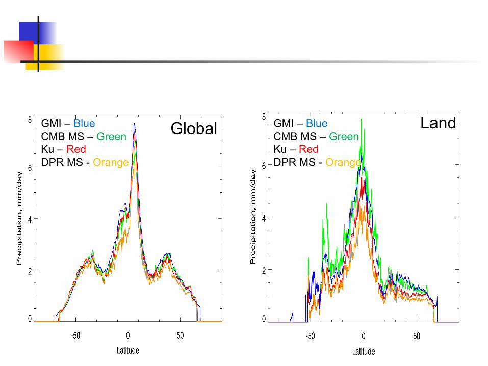
Global GMI – Blue CMB MS – Green Ku – Red DPR MS - Orange

Land GMI – Blue CMB MS – Green Ku – Red DPR MS - Orange

Rain gauges

Radar Dbase w. Ku

Dbase w. CMB MS

-90

-60

-30

0

30

60

90

0 2 4 6 8 10

La#tude

mm/day

ANNUALSNOWFALLMERRASnowSep14-Aug15

ERASnowSep14-Aug15

-90

-60

-30

0

30

60

90

0 2 4 6 8 10

La#tude

mm/day

ANNUALRAINFALLMERRARainSep14-Aug15

ERARainSep14-Aug15

-90

-60

-30

0

30

60

90

0 2 4 6 8 10

La#tude

mm/day

ANNUALTOTALPRECIPITATIONMERRATotalPrecipSep14-Aug15

ERATotalPrecipSep14-Aug15

Neededwork

²  Vertical structure of precipitation over land is still not well captured.

Convective/Stratiform separation or CAPE / other storm organizing characteristics will improve the algorithm

²  Work with Combined Team to make a consistent a-priori database over land

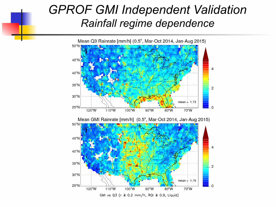
GPROF GMI Independent Validation Rainfall regime dependence

Bias w. Convective Fraction

From Pierre Kirstetter, NOAA, NSSL

TRMM Precipitation Anomalies and ENSO

Deep Organized Regimes

Radiometer Rain Rate Radar Rain Rate

Sat

ellit

e R

ain

Rat

e

Dual-Pol Derived Rain [mm/hr]

From David Henderson

The a-priori database

Radars can use straightforward Z-R relations, except: n  Even when dual frequency observations are available,

radar-only retrievals are uncertain n  Drop size distribution variability is the main source of

uncertainties in reflectivity precipitation relationships n  For small drops the dual frequency equations are identical n  Reflectivity factors may be subject to severe attenuation

The a-priori database (A dual frequency radar/radiometer algorithm)

§  Derive an ensemble of radar-only precipitation retrievals. Variable XR includes: §  Parameterized profiles of particle size distribution

intercepts (Λ) §  Parameterized cloud water and relative humidity

profiles §  Surface emissivity models

§  Simulate brightness temperatures §  Statistically analyze the relationships between

simulated brightness temperatures and XR to derive retrievals consistent with the observations

Ensemble Methodology Formulation

“Basic” DPR+GMI Algorithm Architecture

Upda*ng/FilteringRequired

Obs.GMITB’s

Dual-WavelengthRadar

Algorithm

Obs.Z’s,PIA’s,classifica*on

Es7matedProfilesofPSD’s

TPW,CLWP,PIA,µ, ρice,etc.

SimulateTB’satconstella7on

radiometerchans.andvalidate

offline

RadiometerDatabases

Radia7veTransfer

SimulatedGMITB’s

AgreementwithObservedTB’s?

OK

surfaceemission

FinalEs7matedProfilesofTPW;CLWP,PSD’sρice,etc.,&errors

GMIAntennaPaRernConvolu7on

Consistent Physics / A Priori

Information

EmissivityModule

offline

Prototype Algorithm Architecture (Radar Module)

SRT estimates of PIAKu and PIAKa

analysis of p, T, q, and

CLW profiles

DPR ZKu and ZKa

initial ensemble of q, CLW profiles;

calc. atten. at Ku, Ka

recursively ensemble filter a priori NW,Do using ZKu,Ka

ensemble filter NW, Do profiles using

PIAKu,Ka Output is ensemble of NW,Do profiles consistent with ZKu,Ka and PIAKu,Ka , given q, CLW.

€

n D( ) = Nw f µ( ) DDo

⎛

⎝ ⎜

⎞

⎠ ⎟

µ

exp −3.67+µDo

D⎛

⎝ ⎜

⎞

⎠ ⎟

Precip. size distribution:

2

Ensemble Kalman Filtering Approach

• Assume a priori ensemble, xi, of desired parameter, x.

• Use forward model y = f(x) to simulate observable yi for each xi.

• Update xi using yobs and covariance σxy of xi and yi :

xi’ = xi + σxy / (σyy + σ2noise) • (yobs - yi)

• take mean of xi (solution) and standard deviation of xi (uncertainty).

xi

y = f(x)

xi’ xi’ σx ’ i


8

Prototype Algorithm Architecture

SRT estimates of PIAKu and PIAKa

analysis of p, T, q, and

CLW profiles DPR ZKu and ZKa

initial ensemble of q, CLW profiles;

calc. atten. at Ku, Ka

recursively ensemble filter a priori NW,Do using ZKu,Ka

ensemble filter NW,Do profiles using

PIAKu,Ka

assign Tsfc, emissivities

randomly to DPR-derived

profile ensembles

analysis of Tsfc,

emissivities (U10)

simulate TBGMI using DPR-derived

profile member

filter DPR solutions using Gibbs sampling

procedure

save estimates and uncertainties

GMI TB’s

Output is ensemble of NW, Do, q, CLW profiles and emissivities consistent with ZKu,Ka , PIAKu,Ka , and GMI TB’s.

3

Components -- Default Algorithm

• Radiative Transfer Module

- Eddington’s Second Approximation (Yes)

- inputs: PSD profile parameters (No*, Do, mu, rho-ice);

temperature, humidity, cloud water profiles;

surface skin temperature, emissivities.

- output: brightness temperatures in GMI channels.

Joint Distributions of Surface Rainfall Reference and Retrieved

Why is CMB so low high latitude ocean?

Summaryofneededwork

²  The algorithm Currently uses the non-uniform beam filling that is

different from DPR Ku. Need reconciliation

²  The algorithm starts with radar solutions. If no echo, then no precipitation. Need flexibility to deal consistently with light precipitation that only GMI can detect.

In general

²  Focus more on product availability and assessments to guide future development.

the gpm microwave imager and combined precipitaon algorithms

Documents