The Generalized Brain-State-in-a-Box (gBSB)

Neural Network: Model, Analysis, and

Applications

Cheolhwan Oh and Stanislaw H.Zak

School of Electrical and Computer Engineering

Purdue University

West Lafayette, IN 47907, USA

Email: {oh2, zak}@purdue.edu

Stefen Hui

Department of Mathematical Sciences

San Diego State University

San Diego, CA 92182, USA

Email: hui@saturn.sdsu.edu

Abstract— The generalized Brain-State-in-a-Box (gBSB)

neural network is a generalized version of the Brain-

State-in-a-Box (BSB) neural network. The BSB net is a

simple nonlinear autoassociative neural network that was

proposed by J. A. Anderson, J. W. Silverstein, S. A. Ritz,

and R. S. Jones in 1977 as a memory model based on

neurophysiological considerations. The BSB model gets

its name from the fact that the network trajectory is

constrained to reside in the hypercubeHn = [−1, 1]n.

The BSB model was used primarily to model effects and

mechanisms seen in psychology and cognitive science. It

can be used as a simple pattern recognizer and also

as a pattern recognizer that employs a smooth nearness

measure and generates smooth decision boundaries. Three

different generalizations of the BSB model were proposed

by Hui and Zak, Golden, and Anderson. In particular, the

network considered by Hui and Zak, referred to as the

generalized Brain-State-in-a-Box (gBSB), has the property

that the network trajectory constrained to a hyperface

of Hn is described by a lower-order gBSB type model.

This property simplifies significantly the analysis of the

dynamical behavior of the gBSB neural network. Another

tool that makes the gBSB model suitable for constructing

associative memory is the stability criterion of the vertices

of Hn. Using this criterion, a number of systematic methods

to synthesize associative memories were developed.

In this paper, an introduction to some useful properties

of the gBSB model and some applications of this model

are presented first. In particular, the gBSB based hybrid

neural network for storing and retrieving pattern sequences

is described. The hybrid network consists of autoassociative

and heteroassociative parts. In the autoassociative part,

where patterns are usually represented as vectors, a set

of patterns is stored by the neural network. A distorted

(noisy) version of a stored pattern is subsequently presented

to the network and the task of the neural network is

to retrieve (recall) the original stored pattern from the

noisy pattern. In the heteroassociative part, an arbitrary

set of input patterns is paired with another arbitrary set of

output patterns. After presenting hybrid networks, neural

associative memory that processes large scale patterns in

an efficient way is described. Then the gBSB based hybrid

neural network and the pattern decomposition concept are

used to construct a neural associative memory. Finally,

an image storage and retrieval system is constructed

using the subsystems described above. Results of extensive

simulations are included to illustrate the operation of the

proposed image storage and retrieval system.

I. I NTRODUCTION

James A. Anderson, a pioneer in the area of artificial

neural networks, writes in [1, page 143]: “most memory

in humans is associative. That is, an event is linked to

another event, so that presentation of the first event gives

rise to the linked event.” An associative memory may be

considered a rudimentary model of human memory. In

general, a memory that can be accessed by the storage

address is called an address addressable memory (AAM)

and a memory that can be accessed by content is called

a content addressable memory (CAM) or an associative

memory. When an associative memory is constructed

using a dynamical system, it is called a neural associative

memory. Associative memories can be classified into two

types: autoassociative and heteroassociative memories.

In an autoassociative memory, after prototype patterns

are stored by a neural network, where patterns are

usually represented as vectors, a distorted (noisy) version

of a stored pattern is subsequently presented to the

network. The task of the neural associative memory is

to retrieve (recall) the original stored pattern from its

noisy version. Another type of associative memory is a

heteroassociative memory, where a set of input patterns

is paired with a different set of output patterns. Operation

of a neural associative memory is characterized by two

stages: storage phase, where patterns are being stored by

the neural network, and recall phase, where memorized

patterns are being retrieved in response to a noisy pattern

being presented to the network. In this paper, we present

in a tutorial fashion, the generalized Brain-State-in-a-

Box (gBSB) neural network that is suitable for construc-

tion of associative memories, and then present dynamical

properties of gBSB model and its applications. For other

neural associative memory models see, for example, [2],

[3], [4], [5], [6], [7], [8].

The paper is organized as follows. In Section II, we

introduce the Brain-State-in-a-Box (BSB) neural model.

In Section III, we analyze useful properties of the gBSB

neural network. In Section IV, we present a method

to construct associative memory using the gBSB neural

network. In Section V, we offer a method for designing

large scale neural associative memory using overlapping

decomposition, and show the simulation results of image

storage and retrieval. In Section VI, we propose a neural

system that can store and retrieve pattern sequences, and

present an application to the image storage and retrieval.

Conclusions are found in Section VII. Finally, possible

research projects are listed in Section VIII.

II. B RAIN-STATE-IN-A-BOX (BSB) NEURAL

NETWORK

The Brain-State-in-a-Box (BSB) neural network is

a simple nonlinear autoassociative neural network that

was proposed by J. A. Anderson, J. W. Silverstein,

S. A. Ritz, and R. S. Jones in 1977 [9] as a memory

model based on neurophysiological considerations. The

BSB model gets its name from the fact that the network

trajectory is constrained to reside in the hypercube

Hn = [−1, 1]n. The BSB model was used primarily to

model effects and mechanisms seen in psychology and

cognitive science [1]. A possible function of the BSB

net is to recognize a pattern from a given noisy version.

The BSB net can also be used as a pattern recognizer

that employs a smooth nearness measure and generates

smooth decision boundaries [10]. The dynamics of the

BSB model and its modified models were analyzed by

Greenberg [11], Golden [12], [13], Grossberg [14], Hui

andZak [15], Hakl [16], Hui, Lillo, andZak [17], Lillo

et al. [18], Anderson [1], Perfetti [19], Hassoun [20],

Zak, Lillo, and Hui [21], Chan andZak [22], [23], Park,

Cho, and Park [24]. A continuous counterpart of the

BSB model referred to as the linear system operating

in a saturated mode was analyzed in Li, Michel, and

Porod [25]. We next introduce the concept of linear

associative memory to prepare us for a discussion of

neural associative memories.

A. Linear associative memory

We use a simple linear associative memory to il-

lustrate the concept of associative memory. Suppose

that r mutally orthogonal patternsv(j), j = 1, 2, . . . , r,

v(i)T v(j) = 0 for i 6= j, are to be stored in a memory.

Let V = [v(1) v(2) · · · v(r)] and let

W =r

∑

j=1

v(j)v(j)T = V V T ,

where V T denotes the transpose ofV . Consider the

simple linear system

y = Wx.

If an input presented to the system is one of the stored

patterns, that is,x = v(k), k ∈ {1, 2, . . . , r}, then

y = Wv(k) =

r∑

j=1

v(j)v(j)T v(k)

= v(k)v(k)T v(k) = cv(k),

where c = v(k)T v(k). Thus, we obtained the input

pattern as the output of the system. The above is an

example of an autoassociative memory.

Now, let us consider the case when the input to the

system is a portion of a stored pattern. The following

example is from [26]. Let

v(k) = v(k1) + v(k2)

and assume thatv(k1) and v(k2) are orthogonal

to each other and thatv(k1) is orthogonal to

v(1), . . . ,v(k−1),v(k+1), . . . ,v(r). If the input of the

system isx = v(k1), then

y = Wv(k1)

=r

∑

j=1

v(j)v(j)T v(k1)

= v(k)v(k)T v(k1)

= (v(k1) + v(k2))(v(k1) + v(k2))T v(k1)

= (v(k1) + v(k2))v(k1)T v(k1)

= dv(k),

whered = v(k1)T v(k1). Therefore, the linear associator

recovered the original stored pattern from the partial

input, that is, the linear associator is an example of the

CAM. A limitation of the above system is that when

the patterns are not orthogonal to each other, it does

not retrieve the stored pattern correctly. Also, when the

input vector is a noisy version of the prototype pattern,

the linear associator above is not able to recall the

corresponding prototype pattern.

Next, we introduce the Brain-State-in-a-Box (BSB)

neural network that can be used as an associative mem-

ory. The BSB net can retrieve a certain pattern when its

noisy version is presented as an input to the net.

B. Brain-State-in-a-Box (BSB) neural network model

The dynamics of the BSB neural network are de-

scribed by the difference equation,

x(k + 1) = g(x(k) + αWx(k)), (1)

with an initial conditionx(0) = x0, wherex(k) ∈ Rn

is the state of the BSB neural network at timek, α > 0

is a step size,W ∈ Rn×n is a symmetric weight matrix,

andg : Rn → R

n is an activation function defined as a

standard linear saturation function,

(g(x))i = (sat(x))i =

1 if xi ≥ 1

xi if − 1 < xi < 1

−1 if xi ≤ −1.

(2)

Figure 1 shows sample trajectories of the BSB model

with the weight matrix

W =

1.2 −0.4

−0.4 1.8

. (3)

−1 −0.5 0 0.5 1−1

−0.5

0

0.5

1

x1

x2

Fig. 1: Trajectories of the BSB model with the weight

matrix (3).

The symmetric weight matrix of the BSB net is not

desirable for the design of associative memory. Also, the

ability to control the basins of attraction of the stable

states is another property that makes it easier to design

associative memory. Hui andZak [15] devised a neural

model that has the above properties, which is described

in the following section.

III. G ENERALIZED BRAIN-STATE-IN-A-BOX (GBSB)

NEURAL NETWORK

Three different generalizations of the BSB model

were proposed by Hui andZak [15], Golden [13],

and Anderson [1]. In particular, the network considered

in [15], referred to as the generalized Brain-State-in-a-

Box (gBSB), has the property that the network trajectory

constrained to a hyperface ofHn is described by a

lower-order gBSB type model. This interesting property

simplifies significantly the analysis of the dynamical

behavior of the gBSB neural network. Another tool that

makes the gBSB model suitable for constructing asso-

ciative memory is the stability criterion of the vertices

of Hn proposed in [15]—see also [20] and [26] for

further discussion of the condition. Lillo et al. [18]

proposed a systematic method to synthesize associative

memories using the gBSB neural network. This method

is presented in this paper. For further discussion of the

method to synthesize associative memories using the

gBSB neural network, we refer the reader to [24], [27],

and [28].

A. Model

The gBSB neural network allows for a nonsymmet-

rical weight matrix as well as to offer more control of

the volume of the basins of attraction of the equilibrium

states. The dynamics of the gBSB neural network are

described by

x(k + 1) = g((In + αW )x(k) + αb), (4)

whereg is the standard linear saturation function defined

in (2), In is an n × n identity matrix, b ∈ Rn is

a bias vector, and the weight matrixW ∈ Rn×n is

not necessarily symmetric, which makes it easier to

implement associative memories when using the gBSB

network.

B. Stability

In this section, we discuss stability conditions for the

neural networks presented in the previous section. To

proceed further, the following definitions are needed.

Definition 1: A point xe is an equilibrium state of the

dynamical systemx(k + 1) = T (x(k)) if xe = T (xe).

Definition 2: A basin of attraction of an equilibrium

state of the systemx(k + 1) = T (x(k)) is the set of

points such that the trajectory of this system emanating

from any point in the set converges to the equilibrium

statexe.

In this section, we will be concerned with the equilib-

rium states that are vertices of the hypercubeHn =

[−1, 1]n. That is, equilibrium points that belong to the

set{−1, 1}n.

Definition 3: An equilibrium pointxe of x(k + 1) =

T (x(k)) is stable if for everyε > 0 there is aδ = δ(ε) >

0 such that if‖x(0) − xe‖ < δ then ‖x(k) − xe‖ < ε

for all k ≥ 0, where‖·‖ may be any p-norm of a vector,

for example the Euclidean norm‖ · ‖2.

Definition 4: An equilibrium statexe is super stable

if there exists a neighborhood ofxe, denotedN(xe),

such that for any initial statex0 ∈ N(xe), the trajectory

starting fromx0 reachesxe in a finite number of steps.

Let

L(x) = (In + αW )x + αb

and let (L(x))i be thei-th component of(L(x)). Let

v =[

v1 · · · vn

]T

∈ {−1, 1}n, that is,v is a vertex

of the hypercubeHn. For a vertexv to be an equilibrium

point of the gBSB neural network, we must have

vi = (g(L(v)))i, i = 1, . . . , n.

That is, if vi = 1, then we must have(L(v))i ≥ 1, and

if vi = −1, we must have(L(v))i ≤ −1. Thus, we

obtain the following theorem that can be found in [15].

Theorem 1:A vertex v of the hypercubeHn is an

equilibrium point of the gBSB neural network if and

only if

(L(v))ivi ≥ 1, i = 1, · · · , n.

Using the fact thatv2i = 1 and α > 0, we can restate

Theorem 1 as follows [26].

Theorem 2:A vertex v of the hypercubeHn is an

equilibrium point of the gBSB neural network if and

only if

(Wv + b)ivi ≥ 0, i = 1, · · · , n.

The following theorem, from [17], gives a sufficient

condition for a vertex ofHn to be a super stable

equilibrium state.

Theorem 3:Let v be a vertex of the hypercubeHn.

If

(L(v))ivi > 1, i = 1, · · · , n, (5)

then v is a super stable equilibrium point of the gBSB

neural model.

Proof Because(L(x))ixi is a continuous function, there

exists a neighborhoodN(v) aboutv such that

(L(x))ixi > 1, i = 1, · · · , n and x ∈ N(v).

Therefore, for anyx ∈ N(v), we have

g(L(x)) = v,

which means thatv is indeed a super stable equilibrium

point. �

The sufficiency condition for a pattern to be a super

stable equilibrium state given in the above theorem is

a main tool in the design of associative memories dis-

cussed in this paper. The above condition referred to as

the vertex stability criterion by Hassoun [20, page 411]

is also essential when designing gBSB based associative

memories. We note that such a condition cannot be

obtained for a sigmoidal type of activation function.

Using the fact thatv2i = 1 andα > 0, we can restate

Theorem 3 as follows [26].

Theorem 4:Let v be a vertex of the hypercubeHn.

If

(Wv + b)ivi > 0, i = 1, · · · , n, (6)

then v is a super stable equilibrium point of the gBSB

neural model.

IV. A SSOCIATIVE MEMORY DESIGN USING GBSB

NEURAL NETWORK

In this section, we present a method of designing

associative memory using gBSB neural networks. When

the desired patterns are given, the associative memory

should be able to store them as super stable equilibrium

states of the neural net used to construct the associative

memory. In addition, it is desirable to store the smallest

number of spurious states as possible. We can synthesize

gBSB based associative memories using the method

proposed in [18]. We now briefly describe this method.

For further discussion, see [26].

To proceed, we need the following definitions.

Definition 5: A matrix D ∈ Rn×n is said to be row

diagonal dominant if

dii ≥

n∑

j=1,j 6=i

|dij |, i = 1, · · · , n.

It is strongly row diagonal dominant if

dii >

n∑

j=1,j 6=i

|dij |, i = 1, · · · , n.

Definition 6: GivenV ∈ Rn×r, a matrixV † ∈ R

r×n

is called a pseudo-inverse ofV if

1. V V †V = V ;

2. V †V V † = V †;

3. (V V †)T = V V †;

4. (V †V )T = V †V .

Let v(1), . . . ,v(r) be given vertices ofHn that we

wish to store as super stable equilibrium points of the

gBSB neural network. We refer to these vertices as the

prototype patterns. Then, we have the following theorem:

Theorem 5:Let

V =[

v(1) · · · v(r)]

∈ {−1, 1}n×r.

If

W = DV V †,

where the matrixD satisfies

dii >

n∑

k=1,k 6=i

|dik| + |bi|, i = 1, · · · , n, (7)

thenv(1), . . . ,v(r) are super stable points of the gBSB

neural network.

Proof Using the property of the pseudo-inverse ofV ,

given in Definition 6, we obtain

WV = DV V †V = DV .

Therefore, forj = 1, . . . , r, we have

Wv(j) = Dv(j). (8)

Combining (8) and (6) of Theorem 4, we obtain(

Wv(j) + b)

iv(j)i

=(

Dv(j) + b)

iv(j)i

=

diiv(j)i +

n∑

k=1,k 6=i

dikv(j)k + bi

v(j)i

≥ dii −

n∑

k=1,k 6=i

|dik| − |bi|

> 0.

By Theorem 4,v(j) is super stable. Note that the same

argument holds for anyj = 1, . . . , r and thus the proof

is complete. �

The above result is easy to apply when constructing

the weight matrixW . However, if the diagonal elements

of the matrix D are too large, we may store all the

vertices of the hypercubeHn, which is obviously not

desirable.

The next theorem constitutes a basis for the weight

matrix construction method.

Theorem 6:Let

V =[

v(1) · · · v(r)]

∈ {−1, 1}n×r

be the matrix of the prototype patterns, wherer < n.

Suppose the prototype patterns are linearly independent

so that rank(V ) = r. Let B =[

b · · · b

]

∈ Rn×r

be a matrix consisting of the column vectorb repeated

r times. Let In be then × n identity matrix and let

Λ ∈ Rn×n. Suppose thatD ∈ R

n×n is strongly row

diagonal dominant, that is,

dii >

n∑

k=1,k 6=i

|dik|, i = 1, · · · , n.

If

W = (DV − B)V † + Λ(In − V V †), (9)

then all the patternsv(j), j = 1, . . . , r, are stored as

super stable equilibrium points of the gBSB neural

network.

Proof BecauseV †V = Ir, we have

WV = DV − B,

or

Wv(j) = Dv(j) − b, j = 1, . . . , r.

Therefore,(

Wv(j) + b)

iv(j)i =

(

Dv(j) − b + b)

iv(j)i

=(

Dv(j))

iv(j)i

= dii +n

∑

k=1,k 6=i

dikv(j)k v

(j)i

≥ dii −n

∑

k=1,k 6=i

|dik|

> 0.

Hence, by Theorem 4, each prototype pattern is a

super stable equilibrium point of the gBSB neural

network. �

For further analysis of the formula for the weight

matrix synthesis given by (9), the reader is referred to

[26, pp. 539–542].

The weight matrix construction algorithm is summa-

rized in the following algorithm..

Algorithm 4.1: Weight matrix construction

algorithm

1. For given prototype pattern vectorsv(j) ∈

{−1, 1}n, j = 1, . . . , r, form a matrix B =[

b b · · · b

]

∈ Rn×r, where

b =r

∑

j=1

εjv(j), εj ≥ 0, j = 1, 2, . . . r,

and εj ’s are design parameters.

2. ChooseD ∈ Rn×n such that

dii >

n∑

j=1,j 6=i

|dij |, and

dii <

n∑

j=1,j 6=i

|dij | + |bi|, i = 1, 2, . . . , n,

andΛ ∈ Rn×n such that

λii < −

n∑

j=1,j 6=i

|λij | − |bi|, i = 1, 2, . . . , n,

wheredij and λij are theij-th elements ofD and Λ

respectively.

3. Determine the weight matrixW using the formula

W = (DV − B)V † + Λ(In − V V †),

whereV =[

v(1) · · · v(r)]

∈ {−1, 1}n×r.

4. Implement an associative memory that can store the

given patterns as super stable vertices ofHn using W

andb.

A B C D

Fig. 2: Stored patterns.

We now illustrate the above algorithm with a sim-

ple example using a 25-dimensional gBSB net. We

construct the weight matrix to store the four pattern

vectors corresponding to the bitmaps shown in Figure 2.

The elements of the bitmaps are either 1 (white) or

−1 (black). The pattern vectors are obtained from the

bitmaps by stacking their columns. For example, ifA =[

a1 a2 a3 a4 a5

]

, whereai, i = 1, . . . , 5, is the

i-th column ofA, then the corresponding pattern vector

is obtained fromA by applying the stacking operator

Initial pattern Iteration 1 Iteration 2

Iteration 3 Iteration 4 Iteration 5

Iteration 6 Iteration 7 Iteration 8

Fig. 3: Snapshots of a pattern that converges to a stored

prototype pattern in the gBSB based neural associative

memory.

s : R5×5 → R

25 to get

s(A) = A(:) =

a1

...

a5

∈ {−1, 1}25,

whereA(:) is the MATLAB’s command for the stacking

operation on the matrixA. The weight matrix,W , was

constructed using the above weight matrix construction

algorithm, where

V =[

A(:) B(:) C(:) D(:)]

.

In Figure 3, we show snapshots of the iterations con-

verging towards the letter A of the gBSB neural network

based associative memory.

The above method works well for small size patterns

but is not suitable for large scale patterns. In the next

section, we offer a technique that can effectively process

large scale patterns.

V. L ARGE SCALE ASSOCIATIVE MEMORY DESIGN

USING OVERLAPPING DECOMPOSITION

In this section, we present a gBSB-based method

to design neural associative memories that can process

large scale patterns. A difficulty with large scale neural

associative memory design is the quadratic growth of

the number of interconnections with the pattern size,

which results in a heavy computational load as the

pattern size becomes large. To overcome this difficulty,

we decompose large scale patterns into small size sub-

patterns to reduce the computational overhead. However,

the recall performance of associative memories gets

worse as the size of the neural associative memories

is reduced. To alleviate this problem, we employ the

overlapping decomposition method, which is used to

provide the neural network with the capability of error

detection. We discuss the overlapping decomposition

method in some detail in the following subsection. The

weight matrix of each subnetwork is determined by (9)

independently of its neighboring subnetworks. We add

the error detection and error correction features to our

gBSB associative memory model, which successfully

reduces the number of possible misclassifications. Other

design approaches that use decomposition method can

be found, for example, in [29], [30], [31].

A. Overlapping decomposition

To improve the capabilities of error detection and error

correction and to process the subpatterns symmetrically,

we propose two overlapping decompositions using a ring

structure, suitable for vector patterns, and a toroidal

structure that is suitable for images. We describe these

two decomposition methods next. We begin by decom-

posing a pattern,

v =[

v1 · · · vk vk+1 · · · v2k · · ·

v(p−1)k+1 · · · vpk

]

∈ {−1, 1}pk,

into p subpatterns,

v(1) =[

v1 · · · vk+1

]

∈ {−1, 1}k+1,

v(2) =[

vk+1 · · · v2k+1

]

∈ {−1, 1}k+1,

...

v(p) =[

v(p−1)k+1 · · · vpk

]

∈ {−1, 1}k.

Note thatvk+1 is the overlapping element betweenv(1)

and v(2), v2k+1 betweenv(2) and v(3), and so on.

In this example, each subpattern except forv(1) and

v(p) has two neighboring subpatterns and accordingly,

has two overlapping elements. Each ofv(1) and v(p)

has only one overlapping element. Because the error

detection scheme uses the overlapping elements between

neighboring subnetworks, it is less likely to detect the

errors forv(1) andv(p) than those for other subpatterns.

However if we assume that the decomposition of the

pattern v has a ring structure,v(1) becomes another

neighboring subpattern ofv(p), and vice versa. That is,

v(p) =[

v(p−1)k+1 · · · vpk v1

]

∈ {−1, 1}k+1,

so thatv1 is the overlapping element betweenv(p) and

v(1). In this decomposition, which we refer to as a

ring overlapping decomposition, all subpatterns have the

same dimensions.

We extend the above concept to the case when the pat-

terns are represented by matrices, for example, images.

An example of overlapping decomposition of a matrix

pattern is shown in Figure 4. In Figure 4, the original

pattern is decomposed so that there exist overlapping

parts between neighboring subpatterns.

B. Associative memory with error correction unit

Large scale vector prototype patterns are decomposed

into subpatterns with the ring overlapping decomposition

while images are decomposed using the toroidal over-

lapping decomposition method. Then, the corresponding

individual subnetworks are constructed employing the

1

1

m

2m

pm

1 n n+1 2n+1 qn 12n

m+1

2m+1

V11 V12

V21 V22

V1q

V2q

Vp1 Vp2 Vpq

Fig. 4: An example of toroidal overlapping decomposi-

tion.

method in Section IV independently of other subnet-

works. Each subpattern is assigned to a corresponding

subnetwork as an initial condition. Then, each subnet-

work starts processing the initial subpattern. After all the

individual subnetworks have processed their subpatterns,

the overlapping portions between adjacent subpatterns

are checked. If the recall process is completed perfectly,

all the overlapping portions of the subpatterns processed

by the corresponding subnetworks should match. If a

mismatched boundary is found between two adjacent

subpatterns, we conclude that a recall error occurred

in at least one of the two neighboring subnetworks

during the recall process. In other words, the network has

detected a recall error. Once an error is detected, the error

correction algorithm is used to correct the recall errors.

We next describe a procedure for the case of toroidal

overlapping decomposition. The case of ring overlapping

decomposition is described in [32].

Suppose we are processing an image. Then, every

subpattern overlaps with four neighboring subpatterns

in the decomposition shown in Figure 4. After the

recall process, we check the number of mismatches

Input PatternOriginal

VijijXRecall

ProcessorError Correction

Algorithm

Uij

NijSub−network

ReconstructedOutput Pattern

DecomposedOutput Sub−patterns

DecomposedInput Sub−patterns

Fig. 5: Recall procedure using gBSB-based large scale associative memory with overlapping decompositions and

error correction algorithm when the patterns are in the formof matrices, for example, images.

of the overlapping portions for each subpattern. We

record the number of overlapping portions in which

mismatches occur for each subpattern. The number of

mismatched overlapping portions is an integer from the

set{0, 1, 2, 3, 4}. We first check if there are subpatterns

with no mismatches. If such a pattern is found, the

algorithm is initiated by locating a marker on the above

subpattern and then the marker moves horizontally to

the next subpattern in the same row until a subpattern

with mismatches is encountered. If all subpatterns have

mismatches, we select a subnetwork with the minimal

number of mismatches. Suppose the marker is located

on the subnetworkNij , and assume that the right and

the bottom portions ofV ij have mismatches. Note

that the decomposed input pattern corresponding to the

subnetworkNij is denotedXij . We denote byV ij the

result of the recall process—see Figure 4 and Figure 5

for an explanation of this notation. The (n+1)-th column

of Xij is replaced with the first column ofV i,j+1, and

the (m+1)-th row ofXij is replaced with the first row of

V i+1,j . That is, the algorithm replaces the mismatched

overlapping portions ofXij with the corresponding

portions of its neighboring subpatternsV i,j+1, V i,j−1,

V i+1,j , or V i−1,j , which are the results of the recall

process of the corresponding subnetworks. After the

replacement, the subnetwork goes through the recall

process again and examines the number of mismatches

of the resultant subpattern. If the number of resultant

mismatched portions is smaller than the previous one,

the algorithm keeps this modified result. If the number

of mismatched portions is not smaller than the previous

one, the previous resultV ij is kept. Then, the marker

moves horizontally to the next subnetwork. After the

marker returns to the initial subnetwork, it then moves

vertically to the next row and repeats the same procedure

for the new row. Note that the next row of thep-th

row of the pattern shown in Figure 4 is its first row.

The error correction stage is finished when the marker

returns to the subnetwork that the marker initially started

from. We can repeat the error correction algorithm so

that the subpatterns can go through the error correction

stage multiple times.

The main idea behind the error correction algorithm

is to replace the incorrectly recalled elements of the sub-

pattern with the ones from the neighboring subpatterns

and let the modified subpattern go through the recall

process again. If the elements from the neighboring

subpatterns are correctly recalled, it is more probable

that the current subpattern will be recalled correctly at

the error correction stage. The reason is that we might

have reduced the number of entries with errors and put

the subpattern in the basin of attraction of the prototype

subpattern by replacing the overlapping elements.

C. Storing and retrieving images

We simulated neural associative memory system de-

scribed above using150×150 pixel gray scale images as

patterns. The pixels of original images were represented

with 8 bits. To reduce the computational load, we carried

Fig. 6: Quantized prototype gray scale image patterns.

(a) Input image (b) After recall

(c) After error correction (d) Output image

Fig. 7: An example of a gray scale image retrieval using

the gBSB-based large scale associative memory.

Fig. 8: Quantized prototype color image patterns with 12 bits/pixel.

(a) Input image (b) Result after recall process

(c) Result after error correction process (d) Output image

Fig. 9: Simulation result of image retrieval using the gBSB-based large scale associative memory with color images.

out the uniform quantization so that the quantized images

could be represented with 6 bits per pixel. The number

of levels of the original image is28 = 256, and that

of the quantized image is26 = 64. The simplest way

of uniform quantization would be to divide the range

[0, 255] using 64 intervals of the same length and assign

a binary number with 6 digits to each interval. In this

paper, we used a slightly different way to quantize

images. Instead of dividing the range[0, 255] into the

intervals of the same length, we allocated the same

length to the inner intervals and we assigned half the

length of them to two outermost intervals. The reason

why we used this scheme is because the processed

images had many pixels with extreme values, i.e. 0 and

255. The quantized image patterns are shown in Figure 6.

An example result of the image recall with the gBSB

neural networks is shown in Figure 7. The input image

in Figure 7(a) is a noisy version of a stored image

pattern. The noise in this image is a so called ‘salt-

and-pepper noise’ with error probability of0.5. In other

words, each pixel might be corrupted by a noise with

probability 0.5, and this noisy pixel is white or black

with the same probability. The input image was quan-

tized employing the same method as was used for the

stored image patterns. The whole image pattern was

decomposed into100 (10 × 10) subpatterns using the

overlapping decomposition method described previously.

Each subpattern went through the recall process of the

corresponding subnetwork. The result after the recall

processes of all the subnetworks is shown in Figure 7(b).

There were 5 mismatched portions between subpatterns

in this example. The next stage was the error correction

process. The collection of sub-images in Figure 7(c)

is the result of error correction process. There was no

mismatched portion between these subpatterns. Finally,

the reconstructed image is shown in Figure 7(d). In

this image, there was no erroneously reconstructed pixel

out of 22500 (150 × 150) pixels, that is, no pixel in

the reconstructed image had different values from the

corresponding stored prototype image. More simulation

results involving prototype patterns of Figure 6 can be

found in [33].

We can apply the same procedure to the recall of

color images. We tested the procedure on color images

shown in Figure 8. The pixels in the original images

were represented by 24 bits (8 bits for each of the R,G,B

components) before the uniform quantization preprocess-

ing. The image patterns in Figure 8 are the quantized

versions of the original images with 12 bits per pixel

(4 bits for each of the R,G,B components). An example

of a simulation result is shown in Figure 9. The size of

images used in this simulation was150 × 200 pixels.

The noisy input image in Figure 9(a) was generated for

the simulation in such a way that each of the three R,

G, B matrices were corrupted by zero mean additive

Gaussian noise with standard deviation 2. Note that each

of the R, G, B elements of each pixel has an integer

value in the range[0, 15] in this experiment. The patterns

were decomposed into300 (= 15×20) subpatterns. The

number of mismatched portions between subpatterns was

30 after the recall process, and it was reduced to 0

by the subsequent error correction process. The final

reconstructed image is shown in Figure 9(d). The number

of incorrectly recalled pixels was zero and the prototype

image was perfectly reconstructed.

VI. A SSOCIATIVE MEMORY FORPATTERN

SEQUENCESTORAGE AND RETRIEVAL

In this section, we describe a system that can store

and retrieve images using associative memory that store

and recall pattern sequences.

A. Model

Designing continuous time neural associative memory

that can store pattern sequences has been investigated in

[34], [35], [36], [37], [38], [39]. The discrete time neural

models for storage and recollection of pattern sequences

can be found in [40], [41], [42], [43], [44]. We first

propose a gBSB-based hybrid neural model that can store

and recall pattern sequences and then use this network

to effectively store and retrieve images.

Suppose that we wish to store a sequence of patterns

v1,v2, . . . ,vL in the neural memory in the given order.

Following Lee [39], we represent the sequence of pat-

terns above asv1 → v2 → v3 → · · · → vL to make the

order of patterns clear. It is easy to show that a neural

system described by the following equation can achieve

the storage and retrieval of the pattern sequence,

x(k + 1) = W hx(k), (10)

where the weight matrixW h has the form,

W h = V 2V†1, (11)

where

V 1 =[

v1 v2 v3 · · · vL−1

]

(12)

and

V 2 =[

v2 v3 v4 · · · vL

]

. (13)

Indeed, suppose that the pattern vectors

v1,v2,v3, . . . ,vL−1 ∈ {−1, 1}n are linearly

independent andn ≥ L − 1. In other words,

V 1 ∈ {−1, 1}n×(L−1) and rank V 1 = L − 1.

Then, the pseudo-inverse matrix ofV 1 is equal to the

left pseudo-inverse matrix ofV 1 [45, page 207], that

is,

V†1 = (V T

1 V 1)−1V T

1 . (14)

Note that

W hV 1 = V 2V†1V 1

= V 2(VT1 V 1)

−1V T1 V 1

= V 2.

Therefore,

W hvi = vi+1, i = 1, 2, . . . , L − 1.

Thus, the system (10) generates the output patterns

v2,v3, . . . ,vL for k = 1, 2, . . . , L − 1 in a sequential

manner for the initial inputx(0) = v1. Therefore,

we can store a sequence of patterns by constructing

the weight matrixW h using (11), and retrieve the

whole sequence when a noiseless stored initial pattern

is submitted as an initial condition to the neural system

(10).

In the case when there are more than one sequence of

patterns to store, we can determine the matricesV 1 and

V 2 using the same idea as above. Assume that there are

M sequences of patterns to store,

v(1)1 → v

(1)2 → · · · → v

(1)L1

,

v(2)1 → v

(2)2 → · · · → v

(2)L2

,

· · · · · · · · ·

v(M)1 → v

(M)2 → · · · → v

(M)LM

.

Then, the matricesV 1 andV 2 have the following forms,

V 1 =[

v(1)1 v

(1)2 · · · v

(1)L1−1

... · · ·... v

(M)1 v

(M)2 · · · v

(M)LM−1

]

(15)

and

V 2 =[

v(1)2 v

(1)3 · · · v

(1)L1

... · · ·... v

(M)2 v

(M)3 · · · v

(M)LM

]

. (16)

The number of patterns in each sequence may be differ-

ent from each other. Hence, ifk ≥ Li, i = 1, 2, . . . ,M ,

the neural system (10) might give unexpected outputs.

To prevent this, we modify (15) and (16) as follows:

V 1 =[

v(1)1 v

(1)2 · · · v

(1)L1−1 v

(1)L1

... · · ·... v

(M)1 v

(M)2 · · · v

(M)LM−1 v

(M)LM

]

(17)

and

V 2 =[

v(1)2 v

(1)3 · · · v

(1)L1

v(1)1

... · · ·... v

(M)2 v

(M)3 · · · v

(M)LM

v(M)1

]

. (18)

In this case, the neural system yields the output of the

circular pattern sequence,

v(i)1 → v

(i)2 → · · · → v

(i)Li

→ v(i)1 → v

(i)2 → · · · → v

(i)Li

→ v(i)1 · · · .

The above model works well in the case when there

is no noise in the initial pattern, but it may not work

well with a noisy initial pattern. To overcome this noise

problem, we propose a system whose dynamics are

described as follows:

x(k + 1) = g{(1 − c(k))((In + αW a)x(k) + αb)

+c(k)W hx(k)}, (19)

c(k) =

1 if k = jp − 1, k > 0,

0 if k 6= jp − 1,

(20)

wherek = 0, 1, 2, 3, . . ., j = 0, 1, 2, 3, . . ., p is a fixed

positive integer, and initial conditionx(0) = x0, The

activation functiong, the step sizeα, and the bias vector

b are the same as defined in previous sections. There are

two different weight matrices,W a andW h in (19). The

weight matrixW a is for autoassociation. The synthesis

of the weight matrixW a and the construction of the bias

vector b follow the algorithm described in Section IV.

The weight matrixW h is for heteroassociation. That is,

the transition from one pattern to another is achieved by

W h. The design ofW h follows the method described

above in this section. The role of the functionc(k) in

(19) is to regulate the timing of pattern transitions. When

c(k) = 0, the proposed model acts as a gBSB neural

network, which is an autoassociative neural system, and

whenc(k) = 1, it works as a heteroassociative one. The

transition is set to occur periodically with a periodp as

specified by (20).

When an initial pattern is presented to the neural

system (19), it acts as a gBSB neural system whenk < p.

If the initial pattern is located in the basin of attraction of

a stored pattern, the network trajectory moves toward the

stored pattern ask increases whilek < p. In other words,

{x(0),x(1),x(2), . . . ,x(p− 1)} forms a trajectory that

approaches a prototype super stable equilibrium state.

At k = p, the transition to the next pattern occurs. If

the trajectory reaches the stored prototype pattern while

k < p, the transition atk = p gives the next stored

pattern of the sequence exactly. In this case, noise was

eliminated by the network and the neural system can

retrieve the exact stored pattern sequence afterk = p

with p repetitions of the same pattern. In other words,

if x(p − 1) = v(i)1 , wherev

(i)1 is the first pattern in the

i-th stored pattern sequence, we obtain

x(p) = x(p + 1) = x(p + 2) =

. . . = x(2p − 1) = v(i)2 ,

x(2p) = x(2p + 1) = x(2p + 2) =

. . . = x(3p − 1) = v(i)3 ,

and so on. Consider the case when the initial pattern

does not reach the first stored pattern fork < p, that is,

x(p−1) 6= v(i)1 . Then,x(p) 6= v

(i)2 . In other words,x(p)

is still noisy. But, if x(p) is in the basin of attraction of

v(i)2 , the trajectory approachesv(i)

2 ask increases while

p ≤ k < 2p because now the neural system works as an

autoassociative system for this period. If the trajectory

reaches a prototype patternv(i)2 , the pattern sequence can

be retrieved without noise. In summary, ifx(k) is noisy,

the noise elimination process by the autoassociative part

of the system and the transition to the next pattern by

the heteroassociative part will continue alternately until

noise is eliminated.

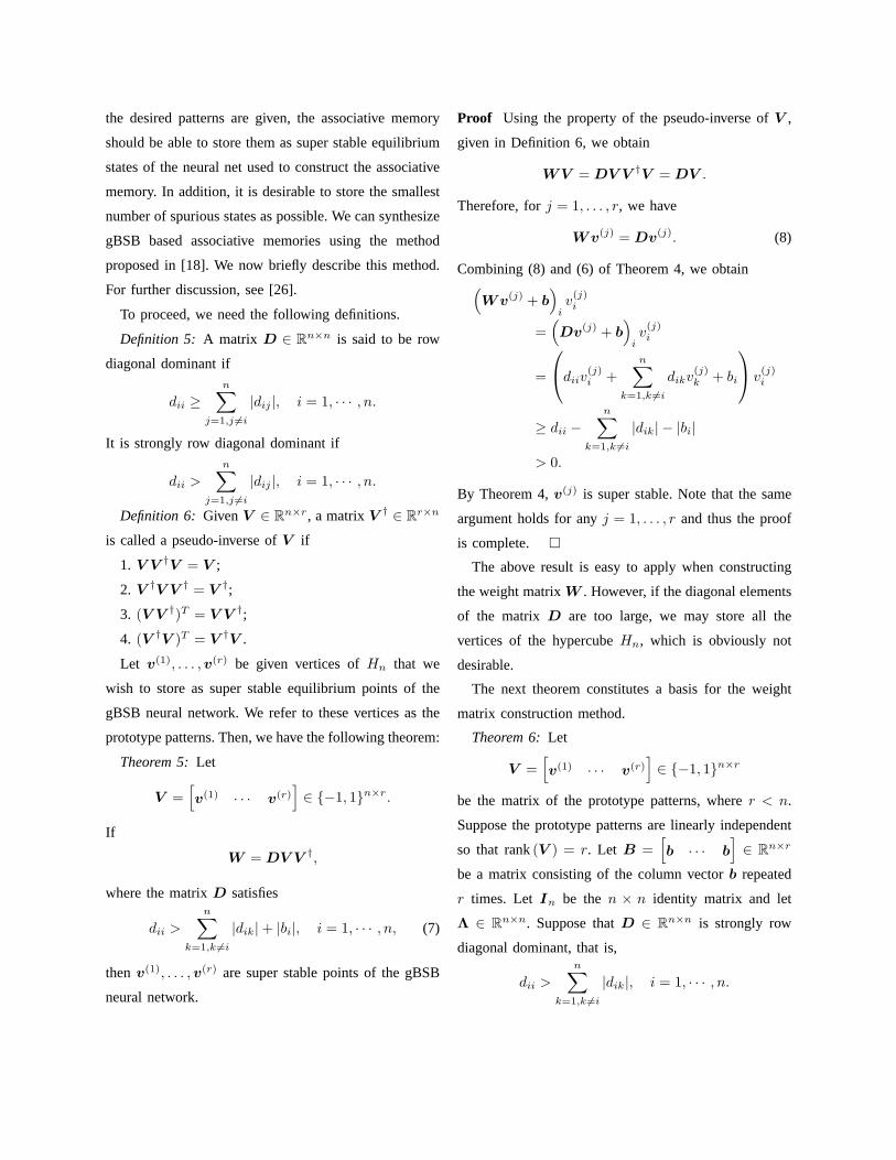
We can modify the above system to speed up the

retrieval process. There existp − 1 redundant patterns

in every p output patterns after the pattern sequence

reaches one of the prototype pattern. We can modify

the function c(k) in (20) to eliminate the redundant

patterns from the output sequence. Oncex(k) reaches

the prototype pattern, the autoassociative iterations will

not change it again and the heteroassociative part alone

can retrieve the pattern sequence successfully in the

subsequent iterations. This can be done by settingc(k) =

1 and fixing it afterx(k) reaches the prototype pattern.

We summarize the above consideration in the following

algorithm.

Algorithm 6.1: Algorithm to eliminate redundant

autoassociative iterations in pattern sequence recall

1. Setflag = 0.

2. Setk = 0.

3. while flag = 0

3.1. If k 6= jp − 1, setc(k) = 0. If k = jp − 1, set

c(k) = 1.

3.2. Calculate

x(k + 1) = g{(1 − c(k))((In + αW a)x(k) + αb)

+c(k)W hx(k)}.

3.3. If x(k + 1) = x(k), setflag = 1.

3.4. Setk = k + 1.

4. Setc(k) = 1 and calculate

x(k + 1) = g{(1 − c(k))((In + αW a)x(k) + αb)

+c(k)W hx(k)}

for the subsequent iterations.

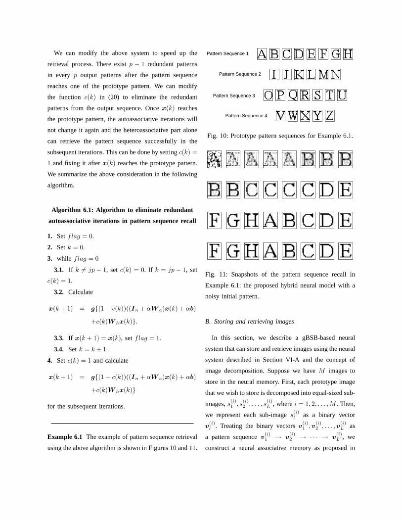
Example 6.1 The example of pattern sequence retrieval

using the above algorithm is shown in Figures 10 and 11.

Pattern Sequence 1

Pattern Sequence 2

Pattern Sequence 3

Pattern Sequence 4

Fig. 10: Prototype pattern sequences for Example 6.1.

Fig. 11: Snapshots of the pattern sequence recall in

Example 6.1: the proposed hybrid neural model with a

noisy initial pattern.

B. Storing and retrieving images

In this section, we describe a gBSB-based neural

system that can store and retrieve images using the neural

system described in Section VI-A and the concept of

image decomposition. Suppose we haveM images to

store in the neural memory. First, each prototype image

that we wish to store is decomposed into equal-sized sub-

images,s(i)1 , s

(i)2 , . . . , s

(i)L , wherei = 1, 2, . . . ,M . Then,

we represent each sub-images(i)l as a binary vector

v(i)l . Treating the binary vectorsv(i)

1 ,v(i)2 , . . . ,v

(i)L as

a pattern sequencev(i)1 → v

(i)2 → · · · → v

(i)L , we

construct a neural associative memory as proposed in

Section VI-A.

When a noisy image is presented to the network, it

is first decomposed intoL equal-sized sub-images and

they are converted into binary vectors. Then, they form a

sequence of vectors to be processed by the neural system

and enter into the stage of the pattern sequence retrieval.

The autoassociative iterations are eliminated at some

point and only heteroassociative steps are necessary

thereafter. Note that the pattern sequence retrieval is

carried out in reverse order of sequence formation. Once

a complete pattern sequence is retrieved, the patterns

included in the sequence are converted back into images.

Finally, we combine those sub-images to obtain the origi-

nal image with the same size as before its decomposition.

We present the snapshots of the simulation result in

Figure 12. The size of image used in this experiment is

160 × 120 and each pixel was represented by a binary

number of 8 bits to give gray level range[0, 255]. The

image was decomposed into 48 sub-images where each

sub-image is a20 × 20 gray scale image. Those 48

sub-images form a pattern sequence. Then, the neural

system proposed above was constructed to store the

prototype images. In this experiment, we added zero

mean Gaussian noise with standard deviation 30 to the

value of each pixel of the prototype image to get an input

image. The input image is shown in Figure 12 (a). This

image was decomposed into 48 sub-images and the im-

age reconstruction started with the autoassociative recall

of the fist sub-image. The numberp was set top = 10.

As we can see in Figure 12 (b), the first sub-image did

not converge to the corresponding prototype sub-image

by k = 9. Because we setp = 10, the heteroassociative

step occurred atk = 10, which is shown in Figure 12 (c).

Then, autoassociative iterations were carried out in the

second sub-image. Because the second sub-image did

not converge to the corresponding prototype sub-image

until k = 19 (Figure 12 (d)), the heteroassociative recall

occurred atk = 20 (Figure 12 (e)). The third sub-image

converged to the prototype sub-image atk = 25 with the

autoassociative recall (Figure 12 (f)). Then,c(k) was

set asc(k) = 1 so that the redundant autoassociative

iterations are not performed in the subsequent recall

process. Fromk = 26, the recall process was performed

with only heteroassociative steps and it stopped atk =

72. The reconstructed image is shown in Figure 12 (l).

Note that the recall of the last sub-image was done at

k = 70 (Figure 12 (j)) but the recall process continued

to complete the recall of the first and the second sub-

images, which was not completed during the previous

pass (Figure 12 (b), Figure 12 (d)). It continued tok =

72 to complete the recall (Figure 12 (k), Figure 12 (l)).

Perfect recall occurred and we successfully reconstructed

the prototype image.

VII. C ONCLUSIONS

In this paper, we first reviewed some properties of

the gBSB neural model that make this network suitable

for using it in constructing associative memories. We

employed the gBSB networks as building blocks in two

different types of associative memory structures that can

store and retrieve images. Both networks use pattern

decomposition. By using pattern decomposition, we were

able to reduce the computational load for processing im-

ages. In the first network, an error correction feature was

added to the system to enhance the recall performance of

the neural memory. In the second system, the concept of

pattern sequence storage and retrieval was used. Because

the autoassociative iteration step can be eliminated after

some number of iterations, this method further reduces

the computation load.

VIII. F URTHER RESEARCH

We are investigating the problem of identification of

the parameters of an autoregressive (AR) time series

(a) k = 0 (input) (b) k = 9 (c) k = 10

(d) k = 19 (e) k = 20 (f) k = 25

(g) k = 26 (h) k = 27 (i) k = 69

(j) k = 70 (k) k = 71 (l) k = 72 (output)

Fig. 12: Snapshots of the recall process of the proposed neural system. (Input image is a noisy version of the

prototype image corrupted by the Gaussian noise.)

model using the gBSB net. The parameters of the model

are determined so that the sum of square errors between

the values of the estimated terms and the actual terms is

minimized. This method is based on the fact that each

trajectory of the gBSB neural model progresses to the

local minimizer of the energy function of the neural net.

The gBSB neural net is designed so that the energy

function of the network is the same as the error function

that is to be minimized. In this particular procedure, the

energy function of the neural network is convex, which

implies that any local minimizer found by the gBSB

algorithm must actually be a global minimizer. Using

the above preliminary results, we are developing an

algorithm for estimating the time series parameters. The

algorithm can then be employed to analyze myoelectric

signals. This method of analyzing myoelectric signals

can then, in turn, be applied to the control of multi-

degree of freedom arm prostheses.

REFERENCES

[1] J. A. Anderson,An Introduction to Neural Networks. Cambridge,

Massachusetts: A Bradford Book, The MIT Press, 1995.

[2] K. Nakano, “Associatron—a model of associative memory,”IEEE

Transactions on Systems, Man, and Cybernetics, vol. 2, no. 3, pp.

380–388, July 1972.

[3] T. Kohonen, “Correlation matrix memories,”IEEE Transactions

on Computers, vol. 21, no. 4, pp. 353–359, April 1972.

[4] T. Kohonen and M. Ruohonen, “Representation of associated data

by matrix operators,”IEEE Transactions on Computers, vol. 22,

no. 7, pp. 701–702, July 1973.

[5] T. Kohonen, “An adaptive associative memory principle,”IEEE

Transactions on Computers, vol. 23, no. 4, pp. 444–445, April

1974.

[6] J. J. Hopfield, “Neural networks and physical systems with

emergent collective computational abilities,”Proc. Natl. Acad.

Sci. USA, Biophysics, vol. 79, pp. 2554–2558, April 1982.

[7] B. Kosko, “Adaptive bidirectional associative memories,” Applied

Optics, vol. 26, no. 23, pp. 4947–4960, December 1987.

[8] P. Kanerva,Sparse Distributed Memory. Cambridge, Mass.:

MIT Press, 1988.

[9] J. A. Anderson, J. W. Silverstein, S. A. Ritz, and R. S. Jones,

“Distinctive features, categorical perception, probability learn-

ing: Some applications of a neural model,” inNeurocomputing;

Foundations of Research, J. A. Anderson and E. Rosenfeld, Eds.

Cambridge, MA: The MIT Press, 1989, ch. 22, pp. 283–325,

reprint fromPsychological Review1977, vol. 84, pp. 413–451.

[10] A. Schultz, “Collective recall via the Brain-State-in-a-Box net-

work,” IEEE Transactions on Neural Networks, vol. 4, no. 4, pp.

580–587, July 1993.

[11] H. J. Greenberg, “Equilibria of the Brain-State-in-a-Box (BSB)

neural model,”Neural Networks, vol. 1, no. 4, pp. 323–324, 1988.

[12] R. M. Golden, “The ”Brain-State-in-a-Box” neural modelis a

gradient descent algorithm,”Journal of Mathematical Psychol-

ogy, vol. 30, no. 1, pp. 73–80, 1986.

[13] ——, “Stability and optimization analyses of the generalized

Brain-State-in-a-Box neural network model,”Journal of Math-

ematical Psychology, vol. 37, no. 2, pp. 282–298, 1993.

[14] S. Grossberg, “Nonlinear neural networks: Principles, mecha-

nisms, and architectures,”Neural Networks, vol. 1, no. 1, pp.

17–61, 1988.

[15] S. Hui and S. H.Zak, “Dynamical analysis of the Brain-State-

in-a-Box (BSB) neural models,”IEEE Transactions on Neural

Networks, vol. 3, no. 1, pp. 86–94, January 1992.

[16] F. Hakl, “Recall strategy of B-S-B neural network,”Neural

Network World, vol. 2, no. 1, pp. 59–82, 1992.

[17] S. Hui, W. E. Lillo, and S. H.Zak, “Dynamics and stability

analysis of the Brain-State-in-a-Box (BSB) neural models,”in

Associative Neural Memories; Theory and Implementation, M. H.

Hassoun, Ed. New York: Oxford University Press, 1993, ch. 11,

pp. 212–224.

[18] W. E. Lillo, D. C. Miller, S. Hui, and S. H.Zak, “Synthesis of

Brain-State-in-a-Box (BSB) based associative memories,”IEEE

Transactions on Neural Networks, vol. 5, no. 5, pp. 730–737,

1994.

[19] R. Perfetti, “A synthesis procedure for Brain-State-in-a-Box

neural networks,”IEEE Transactions on Neural Networks, vol. 6,

no. 5, pp. 1071–1080, September 1995.

[20] M. H. Hassoun,Fundamentals of Artificial Neural Networks.

Cambridge, MA: A Bradford Book, The MIT Press, 1995.

[21] S. H. Zak, W. E. Lillo, and S. Hui, “Learning and forgetting

in generalized Brain-State-in-a-Box (BSB) neural associative

memories,”Neural Networks, vol. 9, no. 5, pp. 845–854, July

1996.

[22] H. Y. Chan and S. H.Zak, “On neural networks that design neural

associative memories,”IEEE Transactions on Neural Networks,

vol. 8, no. 2, pp. 360–372, March 1997.

[23] ——, “Real-time synthesis of sparsely interconnected neural

associative memories,”Neural Networks, vol. 11, no. 4, pp. 749–

759, June 1998.

[24] J. Park, H. Cho, and D. Park, “Design of GBSB neural associative

memories using semidefinite programming,”IEEE Transactions

on Neural Networks, vol. 10, no. 4, pp. 946–950, July 1999.

[25] J. Li, A. N. Michel, and W. Porod, “Analysis and synthesis of a

class of neural networks: Linear systems operating on a closed

hypercube,”IEEE Transactions on Circuits and Systems, vol. 36,

no. 11, pp. 1405–1422, 1989.

[26] S. H. Zak, Systems and Control. New York: Oxford University

Press, 2003.

[27] J. Park and Y. Park, “An optimization approach to design of

generalized BSB neural associative memories,”Neural Compu-

tations, vol. 12, no. 6, pp. 1449–1462, 2000.

[28] F. Sevrani and K. Abe, “On the synthesis of Brain-State-in-a-Box

neural models with application to associative memory,”Neural

Computation, vol. 12, no. 2, pp. 451–472, February 2000.

[29] C. Zetzsche, “Sparse coding: the link between low levelvision

and associative memory,” inParallel Processing in Neural Sys-

tems and Computers, R. Eckmiller, G. Hartmann, and G. Hauske,

Eds. Amsterdam, The Netherlands: Elsevier Science Publishers

B. V. (North-Holland), 1990, pp. 273–276.

[30] N. Ikeda, P. Watta, M. Artiklar, and M. H. Hassoun, “A two-level

Hamming network for high performance associative memory,”

Neural Networks, vol. 14, no. 9, pp. 1189–1200, November 2001.

[31] M. Akar and M. E. Sezer, “Associative memory design using

overlapping decompositions,”Automatica, vol. 37, no. 4, pp.

581–587, April 2001.

[32] C. Oh and S. H.Zak, “Associative memory design using overlap-

ping decomposition and generalized Brain-State-in-a-Box neural

networks,” International Journal of Neural Systems, vol. 13,

no. 3, pp. 139–153, June 2003.

[33] ——, “Image recall using large scale generalized Brain-State-in-

a-Box neural network,”International Journal of Applied Mathe-

matics and Computer Science, vol. 15, no. 1, pp. 99–114, March

2005.

[34] H. Sompolinsky and I. Kanter, “Temporal association in asym-

metric neural networks,”Physical Review Letters, vol. 57, no. 22,

pp. 2861–2864, December 1986.

[35] Y. Baram, “Memorizing binary vector sequences by a sparsely en-

coded network,”IEEE Transactions on Neural Networks, vol. 5,

no. 6, pp. 974–981, November 1994.

[36] M. Morita, “Associative memory with nonmonotone dynamics,”

Neural Networks, vol. 6, no. 1, pp. 115–126, 1993.

[37] ——, “Smooth recollection of a pattern sequence by non-

monotone alalog neural networks,” inProceedings of the IEEE

International Conference on Neural Networks, vol. 2, June 27–

July 2, 1994, pp. 1032–1037.

[38] ——, “Memory and learning of sequential patterns by non-

monotone neural networks,”Neural Networks, vol. 9, no. 8, pp.

1477–1489, November 1996.

[39] D.-L. Lee, “Pattern sequence recognition using a time-varying

Hopfield network,” IEEE Transactions on Neural Networks,

vol. 13, no. 2, pp. 330–342, March 2002.

[40] L. Personnaz, I. Guyon, and G. Dreyfus, “Collective computa-

tional properties of neural networks: New learning mechanisms,”

Physical Review A, vol. 34, no. 5, pp. 4217–4228, November

1986.

[41] I. Guyon, L. Personnaz, J. P. Nadal, and G. Dreyfus, “Storage

and retrieval of complex sequences in neural networks,”Physical

Review A, vol. 38, no. 12, pp. 6365–6372, December 1988.

[42] R. W. Zhou and C. Quek, “DCBAM: a discrete chainable

bidirectional associative memory,”Pattern Recognition Letters,

vol. 17, pp. 985–999, 1996.

[43] D.-L. Lee, “A discrete sequential bidirectional associative mem-

ory for multistep pattern recognition,”Pattern Recognition Let-

ters, vol. 19, pp. 1087–1102, 1998.

[44] L. Wang, “Heteroassociations of spatio-temporal sequences with

the bidirectional associative memory,”IEEE Transactions on

Neural Networks, vol. 11, no. 6, pp. 1503–1505, November 2000.

[45] E. K. P. Chong and S. H.Zak, An Introduction to Optimization,

2nd ed. New York: Wiley-Interscience, John Wiley & Sons,

Inc., 2001.