neural networks - university of illinois at chicagodasgupta/resume/publ/... · artificial neural...
TRANSCRIPT

Neural Networks
Bhaskar DasGupta∗
Department of Computer Science
University of Illinois at Chicago
Chicago, IL 60607
Email: [email protected]
Derong Liu
Department of Electrical & Computer Engineering
University of Illinois at Chicago
Chicago, IL 60607
Email: [email protected]
Hava T. Siegelmann
Computer Science Department
University of Massachusetts
Amherst, MA 01003-9264
Email: [email protected]
August 29, 2005
1 Introduction
Artificial neural networks have been proposed as a tool for machine learning (e.g., see [23, 41, 47, 52]) and
many results have been obtained regarding their application to practical problems in robotics control, vision,
pattern recognition, grammatical inferences and other areas (e.g., see [8, 19, 29, 61]). In these roles, a neural
network is trained to recognize complex associations between inputs and outputs that were presented during
a supervised training cycle. These associations are incorporated into the weights of the network, which encode
∗Supported in part by NSF grants CCR-0206795, CCR-0208749 and IIS-0346973.
1
1 INTRODUCTION 2
a distributed representation of the information that was contained in the input patterns. Once trained, the
network will compute an input/output mapping which, if the training data was representative enough, will
closely match the unknown rule which produced the original data. Massive parallelism of computation, as
well as noise and fault tolerance, are often offered as justifications for the use of neural nets as learning
paradigms.
Traditionally, especially in the structural complexity literature (e.g., see the book [52]), feedforward
circuits composed of AND, OR, NOT or threshold gates have been thoroughly studied. However, in practice,
when designing a neural net, continuous activation functions such as the standard sigmoid are more commonly
used. This is because usual learning algorithms such as the backpropagation algorithm assumes a continuous
activation function. As a result, neural nets are distinguished from those conventional circuits because they
perform real-valued computation and admit efficient learning procedures. The last three decades have seen
a resurgence of theoretical techniques to design and analyze the performances of neural nets (e.g., see the
survey in [36]) as well as novel application of neural nets to various applied areas (e.g., see [19] and some of
the references there). Theoretical researches in computational capabilities of neural nets have given valuable
insights into the mechanisms of these models.
In subsequent discussions, we distinguish between two types of neural networks, commonly known as
the “feedforward” neural nets and the “recurrent” neural nets. A feedforward net consists of a number of
processors (“nodes” or “neurons”) each of which computes a function of the type y = σ(
∑ki=1 aiui + b
)
of
its inputs u1, . . . , uk. These inputs are either external (input data is fed through them) or they represent the
outputs y of other nodes. No cycles are allowed in the connection graph and the output of one designated
node is understood to provide the output value produced by the entire network for a given vector of input
values. The possible coefficients ai and b appearing in the different nodes are the weights of the network, and
the functions σ appearing in the various nodes are the node, activation or gate functions. An architecture
specifies the interconnection structure and the σ’s, but not the actual numerical values of the weights. A
recurrent neural net, on the other hand, allows cycles in the connection graph, thereby allowing the model
to have substantially more computational capabilities (see Section 3.2).

1 INTRODUCTION 3
In this chapter we survey research works dealing with basic questions regarding computational capabilities
and learning of neural models. There are various types of such questions that one may ask, most of them
closely related and complementary to each other. We next describe a few of them informally.
One direction of research deals with the representational capabilities of neural nets, assuming unlimited
number of neurons are available (e.g., see [1, 11, 18, 39, 44, 50, 51]). The origin of this type of research can
be traced back to the work of the famous mathematician Kolmogorov [32], who essentially proved the first
existential result on the representation capabilities of depth 2 neural nets. This type of research ignores the
training question itself, asking instead if it is at all possible to compute or approximate arbitrary functions
(e.g., [11, 32]) or if the net can simulate, say, Turing machines (e.g., [50, 51]). Many of the results and proofs
in this direction are non-constructive.
Another perspective to learnability questions of neural nets takes a numerical analysis or approximation
theoretic point of view. There one asks questions such as how many hidden units are necessary in order to
well-approximate, that is to say, approximate with a small overall error, an unknown function. This type
of research also ignores the training question, asking instead what is the best one could do, in this sense of
overall error, if the best possible network with a given architecture were to be eventually found. Some papers
along these lines are [2, 12], which dealt with single hidden layer nets, and [14], which dealt with multiple
hidden layers.
Another possible line of research deals with the sample complexity questions, that is, the quantification of
the amount of information (number of samples) needed in order to characterize a given unknown mapping.
Some recent references to such work, establishing sample complexity results, and hence “weak learnability”
in the Valiant model, for neural nets, are the papers [3, 17, 20, 35, 38]; the first of these references deals with
networks that employ hard threshold activations, the third and fourth cover continuous activation functions
of a type (piecewise polynomial), and the last one provides results for networks employing the standard
sigmoid activation function.
Yet another direction in which to approach theoretical questions regarding learning by neural networks
originates with the work of Judd (see for instance [26, 27], as well as the related work [5, 33]). Judd was

2 FEEDFORWARD NEURAL NETWORKS 4
motivated by the observation that the “backpropagation” algorithm often runs very slowly, especially for
high-dimensional data. Recall that this algorithm is used in order to find a network (that is, find the weights,
assuming a fixed architecture) that reproduces the observed data. Of course, many modifications of the
vanilla “backprop” approach are possible, using more sophisticated techniques such as high-order (Newton),
conjugate gradient, or sequential quadratic programming methods. However, the “curse of dimensionality”
seems to arise as a computational obstruction to all these training techniques as well, when attempting to
learn arbitrary data using a standard feedforward network. For the simpler case of linearly separable data,
the perceptron algorithm and linear programming techniques help to find a network –with no “hidden units”–
relatively fast. Thus one may ask if there exists a fundamental barrier to training by general feedforward
networks, a barrier that is insurmountable no matter which particular algorithm one uses. (Those techniques
which adapt the architecture to the data, such as cascade correlation or incremental techniques, would not
be subject to such a barrier.)
2 Feedforward Neural Networks
As mentioned before, a feedforward neural net is one in which the underlying connection graph contains no
directed cycles. More precisely, a feedforward neural net (or, in our terminology, a Γ-net) can be defined as
follows.
Let Γ be a class of real-valued functions, where each function is defined on some subset of R. A Γ-net
C is an unbounded fan-in circuit whose edges and vertices are labeled by real numbers. The real number
assigned to an edge (resp. vertex) is called its weight (resp. its threshold). Moreover, to each vertex v a gate
(or activation) function γv ∈ Γ is assigned.
The circuit C computes a function fC : Rm → R as follows. The components of the input vector
x = (x1, . . . , xm) ∈ Rm are assigned to the sources of C. Let v1, . . . , vn be the immediate predecessors of a
vertex v. The input for v is then sv(x) =∑n
i=1 wiyi − tv, where wi is the weight of the edge (vi, v), tv is the
threshold of v and yi is the value assigned to vi. If v is not a sink, then we assign the value γv(sv(x)) to v.

2 FEEDFORWARD NEURAL NETWORKS 5
Otherwise we assign sv(x) to v.
Without any loss of generality, one can assume that C has a single sink t. Then fC = st is the function
computed by C.
The function class Γ quite popular in the structural-complexity literature (e.g., see [21, 22, 46]) is the
binary threshold function H defined by:
H(x) =
0 if x ≤ 0
1 if x > 0
However, in practice this function is not so popular because the function is discrete and hence using this
gate function may pose problems in most commonly used learning algorithms like the backpropagation
algorithms [47] or their variants. Also, from biological perspectives, real neurons have continuous input-
output relations [25]. In practice, various continuous (or, at least locally smooth) gate functions have been
used, for example, the cosine squasher, the standard sigmoid, radial basis functions, generalized radial basis
functions, piecewise-linear, polynomials and trigonometric polynomial functions. In particular, the standard
sigmoid function σ(x) = 1/(1 + e−x) is very popular.
The simplest type of feedforward neural net is the classical perceptron. This consists of one single neuron
computing a threshold function (see Figure 1.1). In other words, the perceptron P is characterized by a
vector (of “weights”) ~c ∈ Rm, and computes the inner product ~c.v + c0 = c1v1 + . . . + cmvm + c0. Such a
model has been well studied and efficient learning algorithms for it exists (e.g., [40], see also [34]). In this
chapter we will be however more interested in more complex multi-layered neural nets.
2.1 Approximation Properties
It is known that neural nets of only depth 2 and with arbitrarily large number of nodes can approximate any
real-valued function upto any desired accuracy, using a continuous activation function such as the sigmoidal
function (e.g., see [11, 32]). However, these proofs are mostly non-constructive and, from a practical point
of view, one is more interested in designing efficient neural nets (i.e., roughly speaking, neural nets with
small size and depth) to exactly or approximately compute different functions. It is also important, from

2 FEEDFORWARD NEURAL NETWORKS 6
a practical point of view, to understand the size-depth tradeoff of the complexity of feedforward nets while
computing functions, since generally neural nets with more layers are more costly to simulate or implement.
Threshold circuits, i.e., feedforward nets with threshold activation functions, have been quite well studied,
and upper/lower bounds for them have been obtained while computing various Boolean functions (see, for
example, [21, 22, 42, 43, 46, 53] among many other works). Functions of special interest have been the parity
function, computing the multiplication and division of binary numbers and so forth.
However, as mentioned before, it is more common in practice to use a continuous activation function,
such as the standard sigmoid function. References [13, 37], among others, considered efficient computation
or approximation of various functions by feedforward circuits with continuous activation functions and also
studied size-depth tradeoffs. In particular, [13] showed that any polynomial of degree n with polynomially
bounded coefficients can be approximated with exponential accuracy by depth 2 feedforward sigmoidal neural
nets with a polynomial number of nodes. References [13, 37] also show how to simulate threshold circuits
by sigmoidal circuits with a polynomial increase in size and a constant factor increase in depth. Thus, in
effect, functions computed by threshold circuits can also be computed by sigmoidal circuits with not too
much increase in size and depth. Maass [35] shows how to simulate nets with piecewise-linear activation
functions with bounded depth, arbitrary real weights, and for Boolean inputs and outputs by a threshold
net of somewhat larger size and depth with weights from −1, 0, 1. References [13, 37] showed that circuits
composed of sufficiently smooth gate functions are capable of of efficiently approximating polynomials within
any degree of accuracy. Complementing these results, reference [13] also provided non-trivial lower-bounds
on the size of bounded-depth sigmoidal nets with polynomially-large weights when computing oscillatory
functions. In essence, one can prove results of the following types.
Definition 1.1 ([13]).1 Let γ : R → R be a function. We call γ non-trivially smooth with parameter k if and
only if there exists rational numbers α, β (α > 0) and an integer k such that α and β have logarithmic size
at most k and
(a) γ can be represented by the power series∑
∞
i=0 ai(x− β)i for all x ∈ [β −α, β +α]. For each i > 1, ai is
1The notation γ(i) denotes the ith derivative of γ.
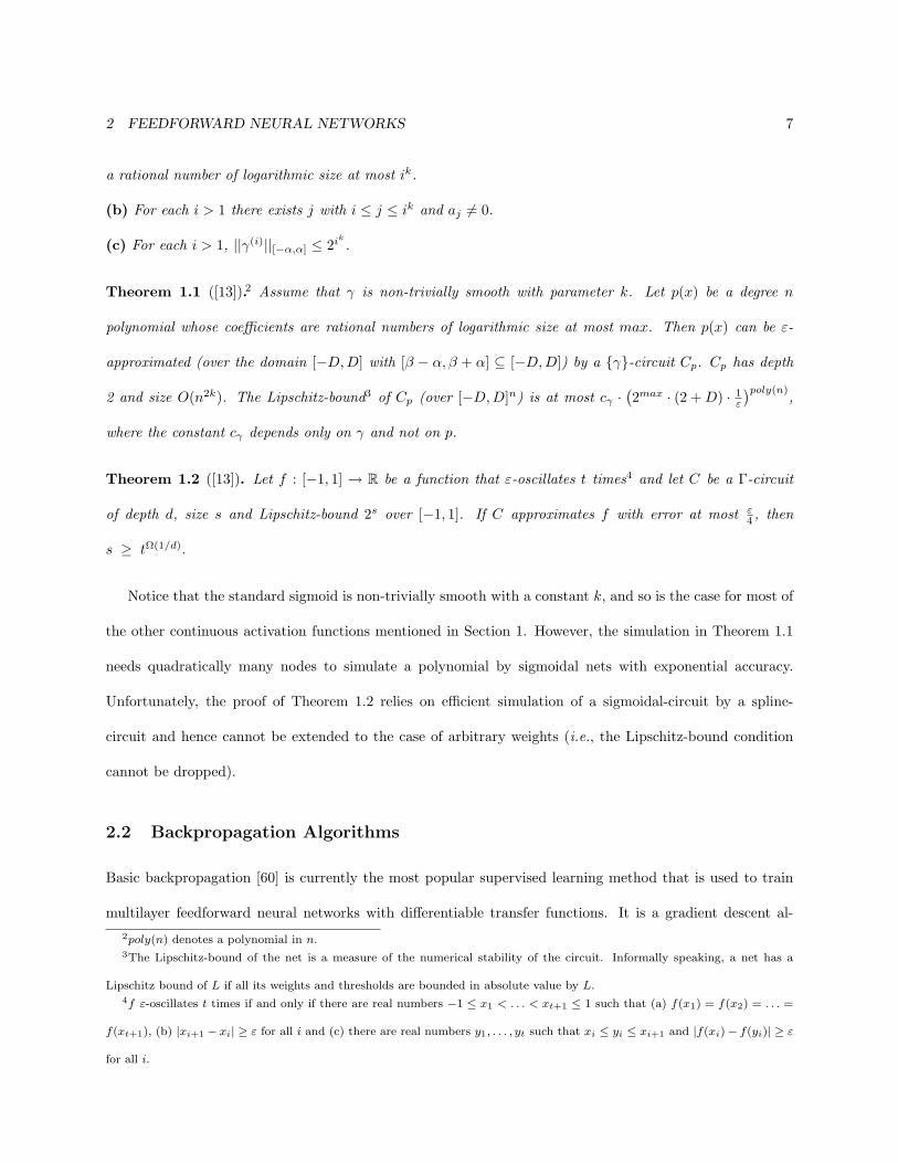
2 FEEDFORWARD NEURAL NETWORKS 7
a rational number of logarithmic size at most ik.
(b) For each i > 1 there exists j with i ≤ j ≤ ik and aj 6= 0.
(c) For each i > 1, ||γ(i)||[−α,α] ≤ 2ik
.
Theorem 1.1 ([13]).2 Assume that γ is non-trivially smooth with parameter k. Let p(x) be a degree n
polynomial whose coefficients are rational numbers of logarithmic size at most max. Then p(x) can be ε-
approximated (over the domain [−D,D] with [β − α, β + α] ⊆ [−D,D]) by a γ-circuit Cp. Cp has depth
2 and size O(n2k). The Lipschitz-bound3 of Cp (over [−D,D]n) is at most cγ ·(
2max · (2 +D) · 1ε
)poly(n),
where the constant cγ depends only on γ and not on p.
Theorem 1.2 ([13]). Let f : [−1, 1] → R be a function that ε-oscillates t times4 and let C be a Γ-circuit
of depth d, size s and Lipschitz-bound 2s over [−1, 1]. If C approximates f with error at most ε4 , then
s ≥ tΩ(1/d).
Notice that the standard sigmoid is non-trivially smooth with a constant k, and so is the case for most of
the other continuous activation functions mentioned in Section 1. However, the simulation in Theorem 1.1
needs quadratically many nodes to simulate a polynomial by sigmoidal nets with exponential accuracy.
Unfortunately, the proof of Theorem 1.2 relies on efficient simulation of a sigmoidal-circuit by a spline-
circuit and hence cannot be extended to the case of arbitrary weights (i.e., the Lipschitz-bound condition
cannot be dropped).
2.2 Backpropagation Algorithms
Basic backpropagation [60] is currently the most popular supervised learning method that is used to train
multilayer feedforward neural networks with differentiable transfer functions. It is a gradient descent al-
2poly(n) denotes a polynomial in n.3The Lipschitz-bound of the net is a measure of the numerical stability of the circuit. Informally speaking, a net has a
Lipschitz bound of L if all its weights and thresholds are bounded in absolute value by L.4f ε-oscillates t times if and only if there are real numbers −1 ≤ x1 < . . . < xt+1 ≤ 1 such that (a) f(x1) = f(x2) = . . . =
f(xt+1), (b) |xi+1 − xi| ≥ ε for all i and (c) there are real numbers y1, . . . , yt such that xi ≤ yi ≤ xi+1 and |f(xi)− f(yi)| ≥ ε
for all i.

2 FEEDFORWARD NEURAL NETWORKS 8
gorithm in which the network weights are moved along the negative of the gradient of the performance
function.
The basic backpropagation algorithm performs the following steps:
1. Forward pass: Inputs are presented and the outputs of each layer are computed.
2. Backward pass: Errors between the target and the output are computed. Then, these errors are
“back-propagated” from the output to each layer until the first layer. Finally, the weights are adjusted
according to the gradient descent algorithm with the derivatives obtained by backpropagation.
We will discuss in more details a generalized version of this approach for recurrent networks, termed as the
“real-time backpropagation through time”, in Section 3.1. The key point of basic backpropagation is that the
weights are adjusted in response to the derivatives of performance function with respect to weights, which
only depend on the current pattern; the weights can be adjusted sequentially or in batch mode. More details
about the basic backpropagation can be found in [60]. The asymptotic convergence rates of backpropagation
is proved in [55]. Traditionally, the parity function has been used as an important benchmark for testing the
efficiency of a learning algorithm. Empirical studies in [54] show that the training time of a feedforward net
using backpropagation while learning the parity function grows exponentially with the number of inputs,
thereby rendering the learning algorithm to be very time-consuming. Unfortunately, a satisfactory theoretical
justification for this behavior is yet to be shown. Also, it is well known that the backpropagation algorithm
may get stuck in local minima, and in fact, in general gradient descent algorithms may fail to classify
correctly data that even simple perceptrons can classify correctly (e.g., see [7, 48, 63]). Strategies of avoiding
local minima include local perturbation and simulated-annealing techniques, whereas the later problem (in
absence of a local minima) can be avoided using, say, threshold LMS procedures.
2.3 Learning Theoretic Results
Approximation results discussed in Section 2.1 does not necessarily translate into good learning algorithms.
For example, even though a sigmoidal net has great computational power, we still need to investigate how to
2 FEEDFORWARD NEURAL NETWORKS 9
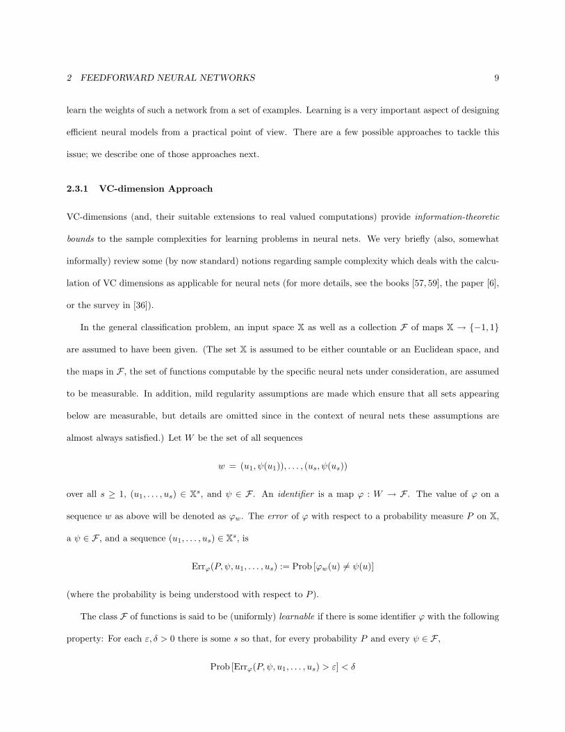
learn the weights of such a network from a set of examples. Learning is a very important aspect of designing
efficient neural models from a practical point of view. There are a few possible approaches to tackle this
issue; we describe one of those approaches next.
2.3.1 VC-dimension Approach
VC-dimensions (and, their suitable extensions to real valued computations) provide information-theoretic
bounds to the sample complexities for learning problems in neural nets. We very briefly (also, somewhat
informally) review some (by now standard) notions regarding sample complexity which deals with the calcu-
lation of VC dimensions as applicable for neural nets (for more details, see the books [57, 59], the paper [6],
or the survey in [36]).
In the general classification problem, an input space X as well as a collection F of maps X → −1, 1
are assumed to have been given. (The set X is assumed to be either countable or an Euclidean space, and
the maps in F , the set of functions computable by the specific neural nets under consideration, are assumed
to be measurable. In addition, mild regularity assumptions are made which ensure that all sets appearing
below are measurable, but details are omitted since in the context of neural nets these assumptions are
almost always satisfied.) Let W be the set of all sequences
w = (u1, ψ(u1)), . . . , (us, ψ(us))
over all s ≥ 1, (u1, . . . , us) ∈ Xs, and ψ ∈ F . An identifier is a map ϕ : W → F . The value of ϕ on a
sequence w as above will be denoted as ϕw. The error of ϕ with respect to a probability measure P on X,
a ψ ∈ F , and a sequence (u1, . . . , us) ∈ Xs, is
Errϕ(P,ψ, u1, . . . , us) := Prob [ϕw(u) 6= ψ(u)]
(where the probability is being understood with respect to P ).
The class F of functions is said to be (uniformly) learnable if there is some identifier ϕ with the following
property: For each ε, δ > 0 there is some s so that, for every probability P and every ψ ∈ F ,
Prob [Errϕ(P,ψ, u1, . . . , us) > ε] < δ
2 FEEDFORWARD NEURAL NETWORKS 10
(where the probability is being understood with respect to P s on Xs).
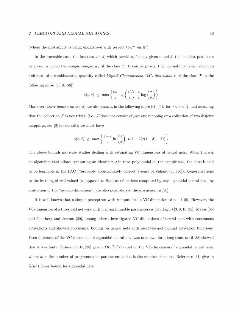
In the learnable case, the function s(ε, δ) which provides, for any given ε and δ, the smallest possible s
as above, is called the sample complexity of the class F . It can be proved that learnability is equivalent to
finiteness of a combinatorial quantity called Vapnik-Chervonenkis (VC) dimension ν of the class F in the
following sense (cf. [6, 58]):
s(ε, δ) ≤ max
8ν
εlog
(
13
ε
)
,4
εlog
(
2
δ
)
Moreover, lower bounds on s(ε, δ) are also known, in the following sense (cf. [6]): for 0 < ε < 12 , and assuming
that the collection F is not trivial (i.e., F does not consist of just one mapping or a collection of two disjoint
mappings, see [6] for details), we must have
s(ε, δ) ≥ max
1 − ε
εln
(
1
δ
)
, ν(1 − 2(ε(1 − δ) + δ))
The above bounds motivate studies dealing with estimating VC dimensions of neural nets. When there is
an algorithm that allows computing an identifier ϕ in time polynomial on the sample size, the class is said
to be learnable in the PAC (“probably approximately correct”) sense of Valiant (cf. [56]). Generalizations
to the learning of real-valued (as opposed to Boolean) functions computed by, say, sigmoidal neural nets, by
evaluation of the “pseudo-dimension”, are also possible; see the discussion in [36].
It is well-known that a simple perceptron with n inputs has a VC-dimension of n + 1 [6]. However, the
VC-dimension of a threshold network with w programmable parameters is Θ(w logw) [3, 9, 10, 35]. Maass [35]
and Goldberg and Jerrum [20], among others, investigated VC-dimensions of neural nets with continuous
activations and showed polynomial bounds on neural nets with piecewise-polynomial activation functions.
Even finiteness of the VC-dimension of sigmoidal neural nets was unknown for a long time, until [38] showed
that it was finite. Subsequently, [28] gave a O(w2n2) bound on the VC-dimension of sigmoidal neural nets,
where w is the number of programmable parameters and n is the number of nodes. Reference [31] gives a
Ω(w2) lower bound for sigmoidal nets.
2 FEEDFORWARD NEURAL NETWORKS 11
2.3.2 The Loading (Consistency) Problem
The VC-dimensions provide information-theoretic bounds on sample complexities for learning. To design an
efficient learning algorithm, the learner should be able to design a neural net consistent with the (polynomi-
ally many) samples it receives. This is known as the consistency or the loading problem. In other words, now
we consider the tractability of the training problem, that is, of the question (essentially quoting Judd [27]):
“Given a network architecture (interconnection graph as well as choice of activation function) and a set of
training examples, does there exist a set of weights so that the network produces the correct output for all
examples?”
The simplest neural network, i.e., the perceptron, consists of one threshold neuron only. It is easily
verified that the computational time of the loading problem in this case is polynomial in the size of the
training set irrespective of whether the input takes continuous or discrete values. This can be achieved via
a linear programming technique. Blum and Rivest [5] showed that this problem is NP-hard for a simple
3-node threshold neural net. References [15, 16] extended this result to show NP-hardness of a 3-node neural
net where the activation function is a simple, saturated piecewise linear activation function, the extension
was non-trivial due to the continuous part of the activation function. It was also observed in [16] that
the loading problem is polynomial-time if the input dimension is constant. However, the complexity of the
loading problem for sigmoidal neural nets still remains an open problem, though some partial results when
the net is somewhat restricted appeared in references such as [24]. Any NP-hardness results of the loading
problems also prove hardness in the PAC learning model, due to the result in [30].
Another possibility to design efficient learning algorithms is to assume that the inputs are drawn according
to some particular distributions. For example, see [4] for efficient learning a depth 2 threshold net with a
fixed number of hidden nodes and with the output gate being an AND gate, assuming that the inputs are
drawn uniformly from a n-dimensional unit ball.

3 RECURRENT NEURAL NETWORKS 12
3 Recurrent Neural Networks
As stated in the introduction, a recurrent neural net allows cycles in the connection graph. A sample
recurrent neural network is illustrated in Figure 1.3.
3.1 Learning Recurrent Networks: Backpropagation Through Time
Backpropagation through time (BPTT) is an approach to solve temporal differentiable optimization problems
with continuous variables [45] and used most often as a training method for recurrent neural networks. In
this section, we describe the method in more details.
3.1.1 Network Definition and Performance Measure
We will use the general expression of Werbos [60] to describe the network dynamics. Symbols y denote node
inputs and outputs, while symbol s denote the weighted sum of node inputs. An ordered set of i, j, l, k on
the weights denotes a connection from node j of layer i to node k of layer l; w0,j,l,k denotes connections
from outside the network. The node activation function is denoted by f(·). The last layer of the network is
denoted by M . The number of nodes in a layer l is denoted by nl. The bias inputs to each node are handled
homogeneously using the connection weights for zeroth input where inputs yext0 (t) and yl−1,0(t) are fixed at
unity for this purpose.
All the algorithms presented in the following part of the chapter are based on the following network
dynamics expressed in pseudo-code format:
for k = 1 to n1
s1,k(t) =
next
∑
j=0
w0,j,1,k(t)yextj (t) +
nM∑
j=1
wM,j,1,k(t)yM,j(t− 1) +
n1∑
j=1
w1,j,1,k(t)y1,j(t− 1) (1.1)
y1,k = f(s1,k(t)) (1.2)
for l = 2 to M

3 RECURRENT NEURAL NETWORKS 13
for k = 1 to nl
sl,k(t) =
nl−1∑
j=0
wl−1,j,l,k(t)yl−1,j(t) +
nl∑
j=1
wl,j,l,k(t)yl,j(t− 1) (1.3)
y1,k = f(s1,k(t)) (1.4)
Note that the input line is not the first layer. Assume that the task to be performed by the network
is sequential supervised learning task, meaning that certain of units’ output values are to match specified
target values at each time step. Define a time-varying ej(t):
ej(t) =
dj(t) − yj(t) if j ∈ layer M
0 otherwise
(1.5)
where dj(t) is the target of the output of the jth unit at time t and define the two performance measure
functions:
J(t) =1
2
∑
k∈M
[ek(t)]2 (1.6)
J total(t0, t) =
t∑
τ=t0
J(τ). (1.7)
3.1.2 Unrolling a Network
In essence, BPTT is the algorithm which calculate derivatives of performance measure with respect to
weights for a feedforward neural network which is obtained by unrolling the network in time. Let N denote
the network which is to be trained to perform a desired sequential behavior. Assume that N has n units and
that it is to run from time t0 up through some time t. As described by Rumelhart et al., we may “unroll”
this network in time to obtain a feedforward network N ∗ which has a layer for each time step in [t0, t] and
n units in each layer. Each unit in N has a copy in each layer of N ∗, and each connection from unit j to
unit i in N has a copy connecting unit j in layer τ to unit i in layer τ + 1, for each τ ∈ [t0, t). An example
of this unrolling mapping is given in Figure 2 in [62]. The key value of this conceptualization is that it

3 RECURRENT NEURAL NETWORKS 14
allows one to regard the problem of training a recurrent network as the corresponding problem of training
a feedforward neural network with certain constraints imposed on its weights. The central result driving
the BPTT approach is that to compute ∂J (t0, t)/∂wij in N one simply computes the partial derivatives of
∂J (t0, t) with respect to each of the τ weights in N ∗ corresponding to wij and adds them up.
Straightforward application of this idea leads to two different algorithm, depending on whether an
epochwise or continual operation approach is sought. One is real-time BPTT and the other is epochwise
BPTT. We only describe the real-time BPTT due to space limitations.
3.1.3 Derivation of BPTT Formulation
Suppose that a differentiable function F expressed in terms of yl,j(τ)|t0 ≤ τ ≤ t, the outputs of the
network over time interval [t0, t] is given. Note while F may have an explicit dependence on yl,j(τ), it may
also have an implicit dependence on this same value through later output values. To avoid the ambiguity in
interpreting partial derivatives like ∂F∂yl,j(τ) , we introduce variable y∗l,j(τ) such that y∗l,j(τ) = yM,j(τ) for all
l = M . Define the following:
ǫl,j(τ) =∂F
∂yl,j(τ), (1.8)
δl,j(τ) =∂F
∂sl,j(τ). (1.9)
Since F depends on yl,j(τ), sl,k(τ + 1) and sl+1,m(τ), we have:
∂F
∂yl,j(τ)=
∂F
∂y∗l,j(τ)+
nl∑
k=1
∂F
∂sl,k(τ + 1)
∂sl,k(τ + 1)
∂yl,j(τ)+
nl+1∑
m=1
∂F
∂sl+1,m(τ)
∂sl+1,m(τ)
∂yl,j(τ)(1.10)
from which we derive the following:
1. τ = t. For this case,
ǫM,j(τ) =∂F
∂y∗M,j(τ)= −ej(τ) (1.11)
where M means the output layer of the network and j ∈ 1, 2, . . . , nM and
ǫl,j(τ) =∂F
∂yl,j(τ)=
nl+1∑
m=1
∂F
∂sl+1,m(τ)
∂sl+1,m(τ)
∂yl,j(τ)=
nl+1∑
m=1
∂F
∂yl+1,m(τ)
∂sl+1,m(τ)
∂yl,j(τ)
∂sl+1,m(τ)
∂yl,j(τ)
=
nl+1∑
m=1
ǫl+1,m(τ)f′
(sl+1,m(τ))wl,j,l+1,m (1.12)
3 RECURRENT NEURAL NETWORKS 15
where l = 1, 2, . . . ,M − 1 and j = 1, 2, . . . , nl, and
δl,j(τ) =∂F
∂sl,j(τ)=
∂F
∂yl,j(τ)
∂yl,j(τ)
∂sl,j(τ)= ǫl,j(τ)f
′
(sl,j(τ)) (1.13)
where l = 1, 2, . . . ,M and j = 1, 2, . . . , nl.
2. τ = t− 1, . . . , t0. In this case,
ǫM,j(τ) =∂F
∂yM,j(τ)=
∂F
∂y∗M,j(τ)+
n1∑
k=1
∂F
∂s1,k(τ + 1)
∂s1,k(τ + 1)
∂yM,j(τ)+
nM∑
k=1
∂F
∂sM,k(τ + 1)
∂sM,k(τ + 1)
∂yM,j(τ)
= −ej(τ) +
n1∑
k=1
δ1,k(τ + 1)wM,j,1,k +
nM∑
k=1
δM,k(τ + 1)wM,j,M,k (1.14)
where M means the output layer M of network and j ∈ 1, 2, . . . , nM,
ǫl,j(τ) =∂F
∂yl,j(τ)=
nl∑
k=1
∂F
∂sl,k(τ + 1)
∂sl,k(τ + 1)
∂yl,j(τ)+
nl+1∑
m=1
∂F
∂sl+1,m(τ)
∂sl+1,m(τ)
∂yl,j(τ)
=
nl∑
k=1
δl,k(τ + 1)wl,j,l,k +
nl+1∑
m=1
∂F
∂yl+1,m(τ)
∂yl+1,m(τ)
∂sl+1,m(τ)
∂sl+1,m(τ)
∂yl,j(τ)
=
nl∑
m=1
δl,k(τ + 1)wl,j,l,k +
nl+1∑
m=1
ǫl+1,m(τ)f′
(sl+1,m(τ))wl,j,l+1,m (1.15)
where l = 1, 2, . . . ,M − 1 and j = 1, 2, . . . , nl and
δl,j(τ) =∂F
∂sl,j(τ)=
∂F
∂yl,j(τ)
∂yl,j(τ)
∂sl,j(τ)= ǫl,j(τ)f
′
(sl,j(τ)) (1.16)
where l = 1, 2, . . . ,M and j = 1, 2, . . . , nl.
In addition, for any appropriate i and j
∂F
∂wi,j,l,k=
t∑
τ=t0
∂F
∂wi,j,l,k(τ)(1.17)
and, for any τ
∂F
∂wi,j,l,k(τ)=
∂F
∂sl,k(τ)
∂sl,k(τ)
∂wi,j,l,k(τ)= δl,k(τ)yi,j(τ) or δl,k(τ)yi,j(τ − 1). (1.18)
Combining these last two equations yields:
∂F
∂wi,j,l,k=
t∑
τ=t0
δl,k(τ)yi,j(τ) or δl,k(τ)yi,j(τ − 1)). (1.19)
Equations (1.11), (1.12), (1.13), (1.14), (1.15), (1.16), and (1.19) represent the BPTT computation of
∂F/∂wi,j,l,k for differentiable function F expressed in terms of the outputs of individual units in the network.
3 RECURRENT NEURAL NETWORKS 16
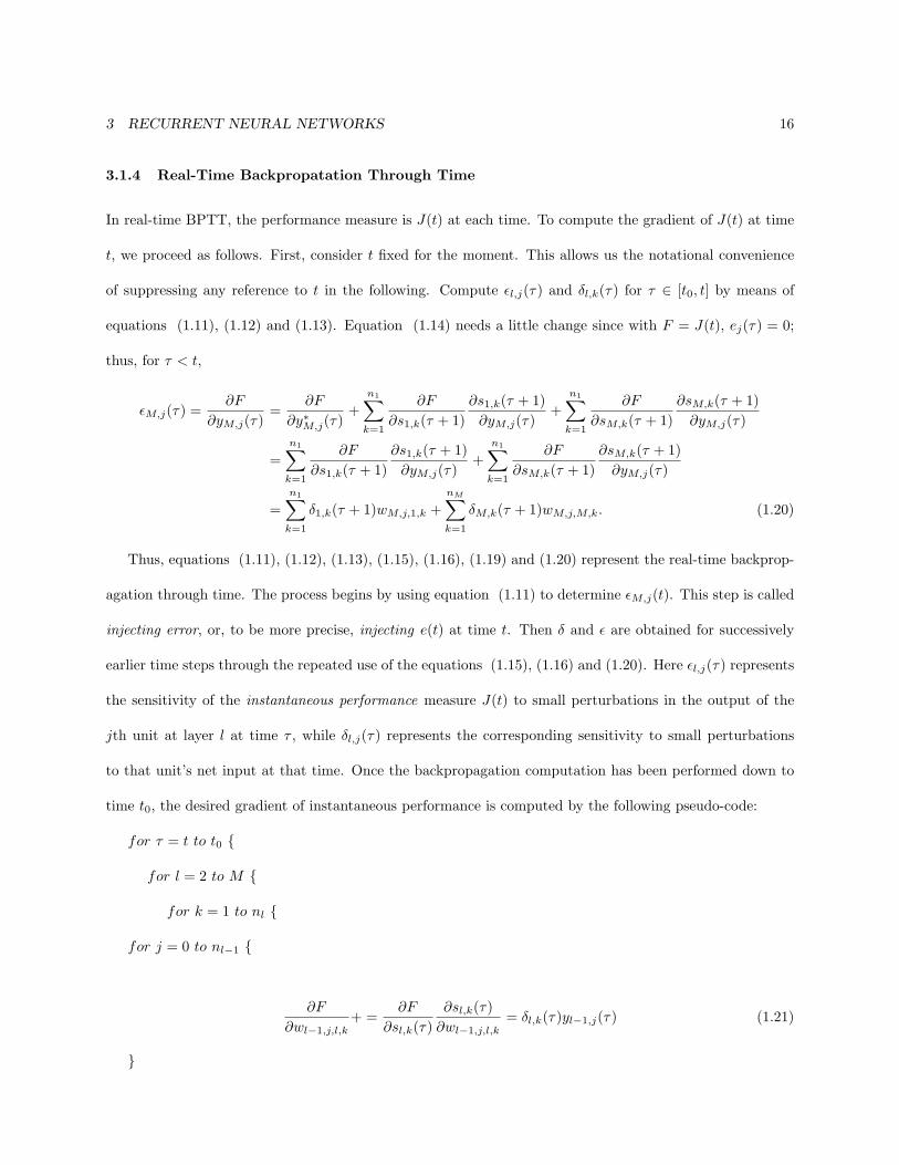
3.1.4 Real-Time Backpropatation Through Time
In real-time BPTT, the performance measure is J(t) at each time. To compute the gradient of J(t) at time
t, we proceed as follows. First, consider t fixed for the moment. This allows us the notational convenience
of suppressing any reference to t in the following. Compute ǫl,j(τ) and δl,k(τ) for τ ∈ [t0, t] by means of
equations (1.11), (1.12) and (1.13). Equation (1.14) needs a little change since with F = J(t), ej(τ) = 0;
thus, for τ < t,
ǫM,j(τ) =∂F
∂yM,j(τ)=
∂F
∂y∗M,j(τ)+
n1∑
k=1
∂F
∂s1,k(τ + 1)
∂s1,k(τ + 1)
∂yM,j(τ)+
n1∑
k=1
∂F
∂sM,k(τ + 1)
∂sM,k(τ + 1)
∂yM,j(τ)
=
n1∑
k=1
∂F
∂s1,k(τ + 1)
∂s1,k(τ + 1)
∂yM,j(τ)+
n1∑
k=1
∂F
∂sM,k(τ + 1)
∂sM,k(τ + 1)
∂yM,j(τ)
=
n1∑
k=1
δ1,k(τ + 1)wM,j,1,k +
nM∑
k=1
δM,k(τ + 1)wM,j,M,k. (1.20)
Thus, equations (1.11), (1.12), (1.13), (1.15), (1.16), (1.19) and (1.20) represent the real-time backprop-
agation through time. The process begins by using equation (1.11) to determine ǫM,j(t). This step is called
injecting error, or, to be more precise, injecting e(t) at time t. Then δ and ǫ are obtained for successively
earlier time steps through the repeated use of the equations (1.15), (1.16) and (1.20). Here ǫl,j(τ) represents
the sensitivity of the instantaneous performance measure J(t) to small perturbations in the output of the
jth unit at layer l at time τ , while δl,j(τ) represents the corresponding sensitivity to small perturbations
to that unit’s net input at that time. Once the backpropagation computation has been performed down to
time t0, the desired gradient of instantaneous performance is computed by the following pseudo-code:
for τ = t to t0
for l = 2 to M
for k = 1 to nl
for j = 0 to nl−1
∂F
∂wl−1,j,l,k+ =
∂F
∂sl,k(τ)
∂sl,k(τ)
∂wl−1,j,l,k= δl,k(τ)yl−1,j(τ) (1.21)

3 RECURRENT NEURAL NETWORKS 17
for j = 1 to nl
∂F
∂wl,j,l,k+ =
∂F
∂sl,k(τ)
∂sl,k(τ)
∂wl,j,l,k= δl,k(τ)yl,j(τ − 1) (1.22)
/*k loop*/ /*l loop*/
for k = 1 to n1
for j = 1 to next
∂F
∂w0,j,1,k+ =
∂F
∂sl,k(τ)
∂sl,k(τ)
∂w0,j,1,k= δ1,k(τ)yext
j (τ) (1.23)
for j = 1 to nM
∂F
∂wM,j,1,k+ =
∂F
∂sl,k(τ)
∂sl,k(τ)
∂wM,j,1,k= δ1,k(τ)yM,j(τ − 1) (1.24)
for j = 1 to n1
∂F
∂w1,j,1,k+ =
∂F
∂sl,k(τ)
∂sl,k(τ)
∂w1,j,1,k= δ1,k(τ)y1,j(τ − 1) (1.25)
/*k loop*/
/*τ loop*/
where the notation “+ =” is to indicate that the quantity on the right hand side of an expression is added
to the previous value (time) of the left hand side. Thus, the sum of ∂F∂wi,j,l,k
from t0 to t is computed. Because
this algorithm makes use of potentially unbounded history storage, it also sometimes called BPTT(∞).
3.2 Computational Capabilities of Discrete and Continuous Recurrent Net-
works
The computational power of recurrent nets is investigated in references such as [50, 51]; see also [49] for a
thorough discussion of recurrent nets and analog computation in general. Recurrent nets include feedforward

REFERENCES 18
nets and thus the results for feedforward nets apply to recurrent nets as well. But recurrent nets gain
considerable more computational power with increasing computation time. In the following, for the sake of
concreteness, we assume that the piecewise-linear function π(x) =
0 if x ≤ 0
x if 0 ≤ x ≤ 1
1 if x ≥ 1
is chosen as activation
function. We concentrate on binary input and assume that the input is provided one bit at a time.
First of all, if weights and thresholds are integers, then each node computes a bit. Recurrent net with
integer weights thus turn out to be equivalent to finite automata and they recognize exactly the class of
regular language over the binary alphabet 0, 1.
The computational power increases considerably for rational weights and thresholds. For instance, a
“rational” recurrent net is, up to a polynomial time computation, equivalent to a Turing machine. In
particular, a network that simulates a universal Turing machine does exist and one could refer to such a
network as “universal” in the Turing sense. It is important to note that the number of nodes in the simulating
recurrent net is fixed (i.e., does not grow with increasing input length).
Irrational weights provide a further boost in computation power. If the net is allowed exponential
computation time, then arbitrary Boolean functions (including non-computable functions) are recognizable.
However, if only polynomial computation time is allowed, then nets have less power and recognize exactly
the languages computable by polynomial-size Boolean circuits.
References
[1] W. Arai, Mapping abilities of three-layer networks, Proceedings of the International Joint Conference
on Neural Networks, 1989, pp. 419-423.
[2] A. R. Barron, Approximation and estimation bounds for artificial neural networks, Proceedings of the
4th Annual Workshop on Computational Learning Theory, Morgan Kaufmann, 1991, pp. 243-249.
REFERENCES 19
[3] E. B. Baum, and D. Haussler, What size net gives valid generalization?, Neural Computation, 1, pp.
151-160, 1989.
[4] A. L. Blum and R. Kannan, Learning and Intersection of k Halfspaces Over a Uniform Distribution,
Proceedings of the 34th Annual Symposium on Foundations of Computer Science, 1993, pp. 312-320.
[5] A. Blum, and R. L. Rivest, Training a 3-node neural network is NP-complete, Neural Networks, 5, pp.
117-127, 1992.
[6] A. Blumer, A. Ehrenfeucht, D. Haussler, and M. Warmuth, Learnability and the Vapnik-Chervonenkis
dimension, Journal of the ACM, 36 (1989), pp. 929-965.
[7] M. Brady, R. Raghavan and J. Slawny, Backpropagation fails to separate where perceptrons succeed,
IEEE Transactions on Circuits and Systems, 26 (1989), pp. 665-674.
[8] G. A. Carpenter and S. Grossberg, A massively parallel architecture for a self-organizing neural pattern
recognition machine, Computer Vision, Graphics, and Image Processing, 37 (1987), pp. 54-115.
[9] T. M. Cover, Geometrical and Statistical Properties of linear threshold elements, Stanford PhD Thesis
1964, Stanford SEL Technical Report No. 6107-1, May 1964.
[10] T. M. Cover, Capacity problems for linear machines, in Pattern Recognition, L. Kanal (editor), Thomp-
son Book Company, 1968, pp. 283-289.
[11] G. Cybenko, Approximation by superposition of a sigmoidal function, Mathematics of Control, Signals,
and System, 2 (1989), pp. 303-314.
[12] C. Darken, M. Donahue, L. Gurvits, and E. D. Sontag, Rate of approximation results motivated by robust
neural network learning, Proceedings of the 6th ACM Workshop on Computational Learning Theory,
1993, pp. 303-309.

REFERENCES 20
[13] B. Dasgupta, and G. Schnitger, The Power of Approximating: A Comparison of Activation Functions,
Advances in Neural Information Processing Systems 5 (C. L. Giles, S. J. Hanson, and J. D. Cowan,
editors), Morgan Kaufmann, San Mateo, CA, 1993, pp. 615-622.
[14] B. DasGupta and G. Schnitger, Analog versus Discrete Neural Networks, Neural Computation, 8, 4
(1996), pp. 805-818.
[15] B. DasGupta, H. T. Siegelmann and E. Sontag, On a Learnability Question Associated to Neural Net-
works with Continuous Activations, Proceedings of the 7th ACM Conference on Learning Theory, 1994,
pp. 47-56.
[16] B. DasGupta, H. T. Siegelmann and E. Sontag, On the Complexity of Training Neural Networks with
Continuous Activation Functions, IEEE Transactions on Neural Networks, 6, 6, (1995), pp. 1490-1504.
[17] B. DasGupta and E. D. Sontag, Sample Complexity for Learning Recurrent Perceptron Mappings, IEEE
Transactions on Information Theory, 42, 5 (1996), pp. 1479-1487.
[18] A. R. Gallant, and H. White, There exists a neural network that does not make avoidable mistakes,
Proceedings of the International Joint Conference on Neural Networks, 1988, pp. 657-664.
[19] C.E. Giles, G.Z. Sun, H.H. Chen, Y.C. Lee, and D. Chen, Higher order recurrent networks and grammat-
ical inference, in Advances in Neural Information Processing Systems 2, D.S. Touretzky (ed.), Morgan
Kaufmann, San Mateo, CA, 1990.
[20] P. Goldberg, and M. Jerrum, Bounding the Vapnik-Chervonenkis dimension of concept classes parame-
terized by real numbers, Proceedings of the 6th ACM Workshop on Computational Learning Theory,
1993, pp. 361-369.
[21] M. Goldmann and J. Hastad, On the power of small-depth threshold circuits, Computational Complexity,
1, 2, pp. 113-129, 1991.
REFERENCES 21
[22] A. Hajnal, W. Maass, P. Pudlak, M. Szegedy and G. Turan, Threshold circuits of bounded depth,
Proceedings of the 28th IEEE Symposium on Foundations of Computer Science, 1987, pp. 99-110.
[23] J. Hertz, A. Krogh and R. G. Palmer, Introduction to the Theory of Neural Computation, Addison
Wesley, 1991.
[24] K-U. Hoffgen, Computational limitations on training sigmoidal neural networks, Information Processing
Letters, 46 (1993), pp. 269-274.
[25] J. J. Hopfield, Neurons with graded response have collective computational properties like those of two-
state neurons, Proceedings of the National Academy of Science USA, 1984, pp. 3008-3092.
[26] J. S. Judd, On the complexity of learning shallow neural networks, Journal of Complexity, 4, pp. 177-192,
1988.
[27] J. S. Judd, Neural Network Design and the Complexity of Learning, MIT Press, Cambridge, MA, 1990.
[28] M. Karpinski and A. Macintyre, Polynomial Bounds for VC Dimension of Sigmoidal and General
Pfaffian Neural Networks, Journal of Computer and Systems Science, 54 (1997), 169-176.
[29] M. Kawato, K. Furukawa and R. Suzuki, A hierarchical neural-network model for control and learning
of voluntary movement, Biological Cybernetics, 57 (1987), pp. 169-185.
[30] M. Kearns, M. Li, L. Pitt and L. Valiant, On the Learnability of Boolean Formulae, Proceedings of the
19th ACM Symposium on Theory of Computing, 1987, pp. 285-295.
[31] P. Koiran and E. D. Sontag, Neural networks with quadratic VC dimension, Journal of Computer and
System Sciences, 54 (1997), pp. 190-198.
[32] A. N. Kolmogorov, On the representation of continuous functions of several variables by superposition
of continuous functions of one variable and addition, Dokl. Akad. Nauk USSR, 114 (1957), pp. 953-956.
[33] J-H. Lin and J. S. Vitter, Complexity results on learning by neural networks, Machine Learning, 6 (1991),
pp. 211-230.
REFERENCES 22
[34] N. Littlestone, Learning Quickly When Irrelevant Attributes Abound: A New Linear-Threshold Algo-
rithm, Proceedings of the 28th Annual Symposium on Foundations of Computer Science, 1987, pp.
68-77.
[35] W. Maass, Bounds for the computational power and learning complexity of analog neural nets, Proceed-
ings of the 25th ACM Symposium on Theory of Computing, 1993, pp. 335-344.
[36] W. Maass, Perspectives of current research about the complexity of learning in neural nets, in Theoretical
Advances in Neural Computation and Learning, V.P. Roychowdhury, K.Y. Siu, and A. Orlitsky (editors),
Kluwer Academic Publishers, 1994, pp. 295-336.
[37] W. Maass, G. Schnitger, and E. D. Sontag, On the computational power of sigmoid versus boolean
threshold circuits, Proceedings of the 32nd Annual Symposium on Foundations of Computer Science,
1991, pp. 767-776.
[38] A. Macintyre, and E. D. Sontag, Finiteness results for sigmoidal ‘neural’ networks, Proceedings of the
25th Annual Symposium on Theory of Computing, 1993, pp. 325-334.
[39] H. N. Mhaskar, Approximation by Superposition of Sigmoidal and Radial Basis Functions, Advances in
Applied Mathematics, 13 (1992), pp. 350-373.
[40] M. Minsky and S. Papert, Perceptrons, The MIT Press, Expanded edition, 1988.
[41] I. Parberry, A Primer on the Complexity Theory of Neural Networks, in Formal Techniques in Artificial
Intelligence: A Sourcebook, R. B. Banerji (editor), Elsevier Science Publishers B. V. (North-Holland),
1990, pp. 217-268.
[42] I. Parberry and G. Schnitger, Parallel computation with threshold functions, Journal of Computer and
System Sciences, 36, 3 (1988), pp. 278-302.
[43] R. Paturi and M. E. Saks, On Threshold Circuits for Parity, Proceedings of the 31st Annual Symposium
on Foundations of Computer Science, 1990, pp. 397-404.

REFERENCES 23
[44] T. Poggio, and F. Girosi, A theory of networks for Approximation and learning, Artificial Intelligence
Memorandum, no 1140, 1989.
[45] D. V. Prokhorov, Backpropagation through time and derivative adaptive critics-a common framework
for comparison, in Handbook of Learning and Approximate Dynamic Programming, Jennies Si, Andrew
G. Barto, W. B. Powell, and Donald Wunsch, Eds., IEEE press pp. 376-404, 2004.
[46] J. H. Reif, On threshold circuits and polynomial computation, Proceedings of the 2nd Annual Structure
in Complexity theory, 1987, pp. 118-123.
[47] D. E. Rumelhart and J. L. McClelland, Parallel Distributed Processing: Explorations in the Microstruc-
ture of Cognition (Volume 1 and Volume 2), The MIT Press, 1986.
[48] Y. Shrivastave and S. Dasgupta, Convergence issues in perceptron based adaptive neural network models,
Proceedings of the 25th Allerton Conference on Communication, Control and Computing, 1987, pp.
1133-1141.
[49] H. T. Siegelmann, Neural Networks and Analog Computation: Beyond the Turing Limit, Birkhauser
publishers, 1998.
[50] H. Siegelmann and E. D. Sontag, Analog computation, neural networks, and circuit, Theoretical Com-
puter Science, 131 (1994), pp. 331-360.
[51] H. Siegelmann and E. D. Sontag, On the computational power of neural nets, Journal of Computer and
System Science 50 (1995), pp. 132-150.
[52] K.-Y. Siu, V. Roychowdhury and T. Kailath, Discrete Neural Computation: A Theoretical Foundation,
Englewood Cliffs, NJ: Prentice Hall, 1994.
[53] K.-Y. Siu, V. Roychowdhury and A. Orlitsky, Lower Bounds on Threshold and Related Circuits via
Communication Complexity, IEEE International Symposium on Information Theory, January, 1992.

REFERENCES 24
[54] G. Teasuro and B. Janssens, Scaling Relationships in Back-Propagation Learning, Complex Systems, 2
(1988), pp. 39-44.
[55] G. Teasuro, Y. He and S. Ahmad, Asymptotic Convergence of Backpropagation, Neural Computation,
1 (1989), pp. 382-391.
[56] L.G. Valiant, A theory of the learnable, Communications of the ACM, 27 (1984), pp.1134-1142.
[57] V.N. Vapnik, Estimation of Dependencies Based on Empirical Data, Springer Verlag, Berlin, 1982.
[58] V.N. Vapnik and A. Ja. Chervonenkis, Theory of Pattern Recognition (in Russian), Moscow, Nauka,
1974. (German translation: W.N. Wapnik and A. Ja. Chervonenkis, Theorie der Zeichenerkennung,
Berlin, Akademia-Verlag, 1979)
[59] M. Vidyasagar, Learning and Generalization with Applications to Neural Networks, Springer Verlag,
London, 1996.
[60] P. J. Werbos, Backpropagation through time:what it does and how to do it, in The Roots of Back-
propation:From Ordered Derivatives to Neural Network and Political Forecasting, Wiley, New York,
Wiley-Interscience Publication pp. 269-294 1994.
[61] B. Widrow, R. G. Winter and R. A. Baxter, Layered neural nets for pattern recognition, IEEE Trans-
actions on Acoustics, Speech and Signal Processing, 36 (1988), pp. 1109-1117.
[62] R. J. Willams and D. Zipser, Gradient-Based learning algorithm for recurrent networks and their compu-
tational complexity, in Backpropagation:Theory, Architectures, and Applications, Y. Chauvin and David
E. Rumelhart, Eds., Hillsdale,New Jersey Larence Erlbaum Associates, Publishers, pp. 433-486, 1994.
[63] B. S. Wittner and J. S. Denker, Strategies for teaching layered networks classification tasks, in Dana
Anderson (editor), Proceedings of Conference on Neural Information Processing Systems, New York,
American Institute of Physics, 1987.

REFERENCES 25
m
*
PPPPq -
HH
HHjc2
cm
c1y
v2v1
vm
(c0)
?
Figure 1.1: Classical Perceptrons
Inputs
Output
Hidden Layers
Figure 1.2: A feedforward neural net with three hidden layers and two inputs
1 2 3
Input Output
Figure 1.3: A simple recurrent network.

Index
Γ-nets, 4
ε-oscillation, 7
Backpropagation through time (BPTT), 12
Basic backpropagation, 7
Binary threshold function, 5
Computational powers of recurrent nets, 17
Feedforward and Recurrent Neural Nets, 2
Lipschitz-bound, 7
Loading problem, 11
Perceptrons, 5
Real-time BPTT, 16
Standard sigmoid function, 5
Threshold circuits, 6
Unrolling a recurrent net, 13
VC dimensions, 9
VC-dimension bounds of neural nets, 10
26