THE FISCAL POLICY IMPACT ON ECONOMIC

PERFORMANCE IN ASEAN5+3:

EMPIRICAL ANALYSES

Pisit Puapan

A Dissertation Submitted in Partial

Fulfillment of the Requirements for the Degree of

Doctor of Philosophy (Economics)

School of Development Economics

National Institute of Development Administration

2011

THE FISCAL POLICY IMPACT ON ECONOMIC

PERFORMANCE IN ASEAN5+3: EMPIRICAL ANALYSES

Pisit Puapan

School of Development Economics

Assistant Professork~~ ,..~ Major Advisor

(Amornrat Apinunmahakul, Ph.D.)

~ ~~Assistant professor. Co-Advisor

(Sasatra Sudsawasd, Ph.D.)

.AssIstant Professor

~ fCX:­ ., .. Co-AdVIsor

(Yuthana Sethapramote, Ph.D.)

The Examining Committee Approved This Dissertation Submitted in Partial

Fulfillment of the Requirements for the Degree of Doctor of Philosophy (Economics).

Assistant Professor !I~ , Committee Chairperson

(Wisarn Pupphavesa, ~

Assistant Professor. ~~ j.~ :Committee

(Amornrat Apinunmahakul, Ph.D.)

Assistant Professor..... ~~...Committee

(Sasatra SUdS~ Assistant Professor Yrl!:.-:. ~~' Committee

(Yuthana Sethapramote, Ph.D.)

Associate professor Deand h.~ l ~: (Adis Israngkura, Ph.D.)

May,2012

ABSTRACT

Title of Dissertation The Fiscal Policy Impact on Economic Performance in

ASEAN5+3: Empirical Analyses Author Pisit Puapan Degree Doctor of Philosophy (Economics) Year 2011

This dissertation consists of two research papers to examine the impact of

fiscal policy on overall economic performance in ASEAN5+3 and Thailand. The

relationship between fiscal policy and economic growth has been a highly contentious

issue among economists. Main economic theories differ in their proposition on the

role of fiscal policy. Classical economics believes that fiscal policy has no long-term

implication on output growth, while Keynesian economics put forth its theory that

fiscal policy does have both temporary and permanent impact on the economy. With

these seemingly opposing views, it is crucial for the policy-makers and the public to

understand the role of fiscal policy particularly taxation and government expenditure

on economic growth. It is imperative for policy-makers to better understand the role

and implication of fiscal policy.

This dissertation titled “The Fiscal Policy Impact on Economic Performance in

ASEAN5+3: Empirical Analyses” comprises of two research studies as follows: 1)

“Assessment of Fiscal Policy Impact on Economic Performances in ASEAN5+3” and

2) “Thailand’s Fiscal Policy Impact Analysis.” The first paper would focus on

examining the role of fiscal policy and economic growth using the panel data for the

five ASEAN countries and the Plus Three countries (China, Japan, and Republic of

Korea) using cross-sectional data during the periods from 1979-2008. This study

classifies fiscal policy into productive versus non-productive expenditure and

distortionary versus non-distortionary taxation to examine in details how fiscal policy

implemented by ASEAN5+3 countries has impacted growth. Other non-fiscal

variables are also included such as domestic investment, international trade, and labor

iv

force. The overall results strongly suggest that fiscal policy in the ASEAN5+3 does

have discernable impact to explain the strong growth performances in the region.

Moreover, economic growth can also be attributed to higher domestic investment,

international trade, and prudent fiscal policy as the underlying factors in supporting

growth in the past decades.

The second paper would focus specifically on Thailand using the Vector

Autoregression (VAR) and Vector Error Correction Model (VECM) methods to

identify the implication of fiscal policy shocks on growth as well as analyze detailed

components of tax and expenditure policies on economic growth in Thailand. The

study finds that, contrary to a priori expectation, the short-run fiscal policy

implemented through tax and public spending does not have significant impact on

economic growth. However, in the longer-term, fiscal policy show discernable

impact on growth particularly tax exhibiting negative impact and government

expenditure showing positive impact on growth. However, in the case of Thailand,

public consumption and its components show positive effects on growth, while public

investment does not seem to have positive impact on economic performance in the

longer-term. This serves as a critical illustration for Thai policy-makers to improve

the productivity of Thailand’s public investment spending in the coming years.

Overall, the main finding of the two researches is that fiscal policy does have

impact on growth in both positive and negative ways. Tax policy generates negative

impact on economic growth in which the government must consider the costs and

benefits of implementing specific tax policies in order to minimize economic

distortions and to ensure that the negative effect from raising the fiscal resources

would be offset by the positive effect after the fiscal resources are deployed through

spending policies. Public expenditures can have positive impact on growth by its

provisions of public goods, infrastructure development, national security, law and

order. However, some public spending generates more positive economic effects than

others. In Thailand, public investment has not generated discernable positive growth

impact on the economy. Public expenditure policy should reorient spending towards

more productive types in order to maximize the positive impact on economic growth

and development. Last but not least, it is hoped that these studies would shed

insightful findings and analyses that would benefit policy-makers in Thailand as well

as the Asian region responsible for fiscal policy formulation for the years to come.

ACKNOWLEDGEMENTS

This dissertation would not have been possible without the guidance and

support of several people who in one way or another graciously extended their

valuable assistance in the completion of this work.

Foremost, I would like to express my warm and sincere gratitude to my

adviser, Assistant Professor Dr. Amornrat Apinunmahakul for her detailed and

constructive comments, and for her patience and constant support throughout this

study. I am deeply grateful to my committees, Assistant Professor Dr. Sasatra

Sudsawasd and Assistant Professor Yuthana Sethapramote, for their insightful

comments and guidance that enabled me to complete my work. Also, I would like to

thank my committee chairperson, Associate Professor Dr. Wisarn Pupphavesa,

Advisor to the Thailand Development Research Institute (TDRI), for his valuable

contribution in finalizing my work. In completing my work, I am also thankful to

various officials at the National Economic and Social Development Board (NESDB)

and Ministry of Finance (MOF) for their facilitation in providing all the necessary

data that makes this research work possible.

I would like to also extend my sincere appreciation to the faculty members at

the School of Development Economics at the National Institute of Development

Administration (NIDA) for their contribution in advancing my knowledge in the past

6 years of my PhD study. This dissertation is dedicated to my parents who have

always encouraged me to learn and improve myself. I am indebted to my family for

their constant support in every aspect throughout my life. My special gratitude is due

to my dear friend, Dr. Pat Pattanarangsun, for his generosity and kindness to me both

academically and personally. Last but not least, I also wish to thank my wife for her

understanding in letting me pursue my academic goal, and my newly born son,

Pongsit, whom I most eagerly look forward to spend with my time with after the

completion of my study.

Pisit Puapan

June 2012

TABLE OF CONTENTS

Page

ABSTRACT iii

ACKNOWLEDGEMENTS v

TABLE OF CONTENTS vi

LIST OF TABLES viii

ESSAY 1 ASSESSMENT OF FISCAL POLICY IMPACT 1

ON ECONOMIC PERFORMANCES IN ASEAN5+3

ABSTRACT 1

CHAPTER 1 INTRODUCTION 2

Background and Research Motivation 4

CHAPTER 2 LITERATURE REVIEW 7

2.1 Taxation and Economic Growth 7

2.2 Government Expenditures and Economic Growth 12

2.3 Fiscal Balance and Economic Growth 15

2.4 Investment and Economic Growth 17

2.5 Education and Economic Growth 20

2.6 Population and Economic Growth 22

2.7 Economic Growth in the Asian Context 24

CHAPTER 3 THEORETICAL MODEL AND METHODOLOGY 26

Methodology 27

CHAPTER 4 DATA DESCRIPTION AND ANALYSIS 32

CHAPTER 5 EMPIRCAL RESULTS 55

Conclusion and Policy Recommendations 59

BIBLIOGRAPHY 62

APPENDIX Summary of Data Statistics 70

vii

ESSAY 2 THAILAND’s FISCAL POLICY IMPACT ANALYSIS 83

ABSTRACT 83

CHAPTER 1 INTRODUCTION 84

Background and Research Motivation 85

CHAPTER 2 LITERATURE REVIEW AND THEORETICAL 89

MODEL AND METHODOLOGY

Conceptual Framework and Methodology 97

CHAPTER 3 FISCAL POLICY IN THAILAND: OVERVIEW, DATA 102

DESCRIPTION AND ANALYSIS 3.1 Overview of Fiscal Policy in Thailand 102

3.2 Data Description and Analysis 105

3.3 Empirical Models and Results 118

BIBLIOGRAPHY 145

APPENDIX 149

BIOGRAPHY 176

viii

LIST OF TABLES

Tables Page

ESSAY 1

4.1 Data Classification by Country 32

4.2 Fiscal Data Classifications 40

5.1 Summary of ASEAN5+3 Results 56

5.2 Summary of ASEAN5 Results 58

ESSAY 2

3.1 Data Sources 106

3.2 Augmented Dickey-Fuller Test Statistic 129

3.3 Co-Integration Test Results 131

ESSAY 1

ASSESSMENT OF FISCAL POLICY IMPACT ON ECONOMIC PERFORMANCES IN ASEAN5+3

ABSTRACT

Previous studies have emphasized on the role of public sector in promoting rapid growth among the ASEAN5+3 countries. In East Asia, the role of the State is assumed to have played active role in channeling resources toward productive uses, and hence enhancing economic growth This study aims to test this proposition using the panel data for the five ASEAN countries (Thailand, Singapore, Indonesia, Malaysia and the Philippines) and the Plus Three countries (China, Japan, and Republic of Korea) in the periods ranging from 1979-2008. This study classifies fiscal policy into productive versus non-productive expenditure and distortionary versus non-distortionary taxation to examine in details how fiscal policy implemented by ASEAN5+3 countries has impacted growth. Other non-fiscal variables are also included such as domestic investment, international trade, and labor force. The overall results strongly suggest that fiscal policy in the ASEAN5+3 does have discernable impact to explain the strong growth performances in the region. Moreover, economic growth can also be attributed to higher domestic investment, international trade, and prudent fiscal policy as the underlying factors in supporting growth in the past decades. Prudent fiscal policy is crucial to economic growth because excessive fiscal deficits can lead to crowding out of private investment, higher interest rate, and real exchange rate appreciation. These findings are mostly consistent with Bleaney, Gemmell and Kneller (2001) for OECD countries where productive expenditure and distortionary taxation also show positive and negative effects on growth, respectively. The study, therefore, suggests that the role of public sector and fiscal policy in ASEAN5+3 should be carefully analyzed as it has strong potentials to affect growth performances either positively and negatively with the aim to achieve better growth results in the coming years.

CHAPTER 1

INTRODUCTION

The subject of economic growth is one of the most intensely studied and

debated in the field of economics. Certainly, the growth process can be readily

observed by rising income and standard of living of the people. Many countries have

experienced unprecedented growth particularly among the North-east and South-east

Asian economies that have consistently recorded close to double-digit GDP growth in

the past few decades.

However, economic progress should not be taken for granted. Some countries

have seen little or no growth over the years such as the Sub-Saharan African and

Caribbean nations, while a few others have seen their living standards have actually

declined compared to their prior generation. Material well-being can therefore be

readily seen and observed, but less is clear about how it can come about.

One of the most controversial issues on economic growth is how the role of

the government and public sector can affect economic growth. In 1956, Robert M.

Solow proposed what is now called neoclassical growth model that the long-run

growth rate is driven by population growth and the rate of technological progress.

Based on his proposition, government policies through taxation and expenditure may

affect the incentive to invest in human or physical capital, but in the long-run this

affects only the equilibrium factor ratios, not the growth rate, although in general

there will be transitional growth rates. Therefore, fiscal policy may only have the

“level effect” on economic growth, but not the “growth effect.” On the other hand,

more recent theoretical growth model particularly the endogenous growth theory

proposed by Robert Barro in 1990 predicts that, among other things such as scale

economies, research and development, there are certain types of taxation and

expenditures that can determine long-run growth rate in a given economy.

Given these contrasting theoretical views, economists are keen to better

understand the key determining factors of economic growth particularly on the role of

3

fiscal policy which are crucial to economic policy formulation. Would productive

investments in physical infrastructure such as road and railway and social

infrastructure such as public education and public health help to promote growth in a

country?

Thus, this study aims to examine and empirically analyze the growth impact of

fiscal policy using panel data from selected 8 countries under the ASEAN Five and

Plus Three countries (China, Japan, South Korea, Thailand, Singapore, Indonesia,

Malaysia, and the Philippines) from periods ranging from 1979 to 2008. The

methodologies used are two-way fixed effect model (Least Square Dummy Variables),

dynamic fixed effect model, and Generalized Methods of Moment (GMM). Fiscal

policy components are classified into productive versus non-productive expenditure

and distortionary versus non-distortionary taxation to examine in details how fiscal

policy by ASEAN5+3 countries could impact growth. The definition of particular

expenditures as productive or non-productive or particular taxes as distortionary or

non-distortionary may be open to debate. However, in this study, the theoretical

classification of tax and public expenditures are based on Professor Barro (1990)

classification. Distortionary taxation and productive investments are those that affect

incentive to invest in human or physical capital. Income-based taxes are considered to

be distortionary in the sense that it affected work incentive, while consumption-based

taxes have relatively less effect on labor-leisure choices. Productive expenditures are

those spending that could increase economic capacity and productivity, while non-

productive expenditures are consumption-type such as social security and welfare

spending. Other non-fiscal variables are also included such as domestic investment,

international trade, and labor force. Previous study by Bleaney et al. (2001) only

includes the two non-fiscal variables, but ASEAN+3 growth may also come from

international trade openness, so export-import to GDP is included as a proxy for trade

openness. There are other measures of openness to trade as well such as average tariff

rate that could potentially be used as the non-fiscal explanatory variable, but due to

data limitation, only export-import to GDP will be used in this study. Human capital

formation is also important to growth in ASEAN+3, so school enrollment ratio is

included as proxy for human capital. Dummy variable for 1997 Asian financial crisis

is also included.

4

Contrary to conventional wisdom, the results strongly suggest that the fiscal

policy implemented in the ASEAN5+3 does have discernable impact to explain the

growth performances in the region. Moreover, the region’s economic growth can also

be attributed to other factors as well particularly domestic investment, international

trade, and prudent fiscal policy as the underlying factors in supporting growth in the

past decades. These findings are different from Bleaney et al. (2001) for OECD

countries where productive expenditure and distortionary taxation also show positive

and negative effects on growth, respectively. The study, therefore, suggests that the

role of public sector and fiscal policy in ASEAN5+3 should be carefully analyzed as

it has strong potentials to affect growth performances either positively and negatively

with the aim to achieve better growth results in the coming years.

Background and Research Motivation

In Asia, the role of fiscal policy in promoting economic growth has been

controversial in whether the Asian States have had a positive role in promoting

growth or active policies implemented by these countries have been growth-neutral or

even growth-inhibiting. The economic core of Asia is now gravitated towards the

Eastern part of the continent with the major driving force in the regional formation

called ASEAN+3 which started in 1997 after the Asian financial crisis comprising of

13 member countries (the 10 ASEAN countries and China, Japan, and South Korea).

Many countries outside regions are closely observing the developments within

ASEAN+3 given its increasing economic power, new and innovative cooperation in

trade and finance, and the future prospect for the eventual formation of East Asia

Economic Community in the years ahead.

By all accounts, economic data in ASEAN+3 have shown that economic

performances in the region have been consistently outperformed other regions. This

phenomenon then offers one of the most interesting inquiries for policy-makers and

professional economists to identify the growth contributors for ASEAN+3 region.

These economies have grown impressively over a period of nearly 30 years. The

region now has 2.17 billion people representing over 30 percent of world population.

In 1960, the GDP of ASEAN+3 was approximately 40 percent of US GDP, with

5

Japan contributing more than 80 percent of total East Asian GDP, followed by China

(Mainland only), with not quite 8 percent. By 2000, the GDP of ASEAN+3 was

approximately 75 percent of US GDP, with Japan contributing more than 60 percent

of total GDP, followed by China (Mainland only), which contributed somewhat more

than 15 percent. Ten years later, China would become the second largest economy in

the world, overtaken Japan and second only to the U.S. Real per capita GDP

expanded in excess of four times during the period, while average global income

registered less than a two-fold increase. Such robust, prolonged growth has clearly

raised incomes, lifted millions out of poverty, and expanded ASEAN+3 region’s

global economic influence.

Per capita GDP in ASEAN+3 remains below the global average at $6,837, but

is rapidly catching up. In 1980, the income of the average person living in ASEAN+3

region was just over a quarter of the world average; by 2010, it had risen to nearly

three-fourth. As in all world regions, the wealth of individual ASEAN+3 countries

differs widely between, and within, states. This is due to its vast size, meaning a huge

range of differing cultures, environments, historical ties and government systems. The

largest economies within ASEAN+3 in terms of nominal GDP are China, Japan,

South Korea, and Indonesia. In terms of GDP by purchasing power parity, China

followed by Japan, and South Korea are the largest economies in decreasing order.

Wealth (if measured by GDP per capita) is mostly concentrated in Northeast

Asian territories such as Hong Kong, Japan, South Korea, Singapore and Taiwan.

Within ASEAN+3, with the exception of Japan, South Korea, Hong Kong and

Singapore, is currently undergoing rapid growth and industrialization spearheaded by

China – one of the fastest growing major economies in the world. Over the years,

with rapid economic growth and large trade surplus with the rest of the world,

ASEAN+3 has accumulated over USD 5.5 trillion of foreign exchange reserves -

more than half of the world's total.

Sustained and rapid growth in ASEAN+3 in the past five decades (1960s

onward) needs analyses to explain the growth determinants. In the current literature

of growth theory, the neoclassical growth model of Solow (1956) postulates that long-

run growth rate is driven by population growth and the rate of technological progress.

Fiscal policy implemented through taxation and government expenditures may affect

6

the incentive to invest in human and physical capital, but it only affects the

equilibrium ratios, not growth rate, in the long-run. On the other hands, endogenous

growth models proposed by Barro, King and Rebelo (1990) predicts that fiscal policy

will affect long-run growth rate. Government spending and taxation should have both

temporary and permanent effects on growth. In particular, fiscal policy in the

endogenous growth model is often classifies into various categories of taxations and

public expenditures to examine growth implications.

This paper aims to develop on the theoretical framework of endogenous

growth model to test for the underlying factors contributing to economic growth

among the ASEAN5 (Thailand, Singapore, Indonesia, Malaysia and the Philippines)

and the Plus Three countries (China, Japan, and Republic of Korea) (hereafter called

“ASEAN5+3”) in the periods ranging from 1979-2008. A particular focus is given to

the role of fiscal policy through public expenditure and taxation implemented by

ASEAN5+3 in their respective impact on economic growth. However, this study will

expand from Bleaney et al. (2001) by examining the role of non-fiscal variables

beyond those covered by the previous study to include the role of trade openness and

education as non-fiscal determinants of growth in the region.

CHAPTER 2

LITERATURE REVIEW

2.1 Taxation and Economic Growth

The starting point of conventional economic growth theorization is the

neoclassical model of Solow (1956). The basic assumptions of the model are: constant

returns to scale, diminishing marginal productivity of capital, exogenously determined

technical progress and substitutability between capital and labor. As a result, the

model highlights the savings or investment ratio as important determinant of short-run

economic growth. Technological progress, though important in the long-run, is

regarded as exogenous to the economic system. In this model, the incentives to save

or to invest in new capital are affected by fiscal policy; this alters the equilibrium

capital-output ratio and therefore the level of the output path, but not its slope (with

transitional effects on growth as the economy moves onto its new path).

On the other hand, endogenous growth models “endogenize” the role of

technological progress as a key driver of long–run economic growth with both

constant and increasing returns to capital. These new growth theories propose that the

introduction of new accumulation factors, such as knowledge, innovation, etc., will

induce self-maintained economic growth. Triggered by Romer’s (1986) and Lucas’

(1988) seminal studies, work within this framework highlighted three significant

sources of growth: new knowledge particularly in the presence of positive externalities

from human capital accumulation (Romer, 1990, Grossman and Helpman, 1991),

endogenous technological change and innovation (Aghion and Howitt, 1992) and

permanent changes in variables potentially affected by government policies lead to

permanent changes in growth rates (i.e. public infrastructure) (Barro, 1990).

Following this third source of growth, the novel feature of the public-policy

endogenous growth models of Barro (1990), Barro and Sala-i-Martin (1992) and

8

Mendoza, Milesi-Ferretti, and Asea (1997) is that fiscal policy can determine both the

level of the output path and the steady-state growth rate.

There are various studies that have examined the relationship between fiscal

policy and growth. A recent study titled Testing the endogenous growth model:

public expenditure, taxation, and growth over the long run by Bleaney et al. (2001)

examines the endogenous growth model to observe the relationship among public

expenditure, taxation and growth over the long-run using the data from OECD

countries during the period from 1970-1995. They have found strong support for

endogenous growth model and suggest that long-run fiscal effects have impact on

growth performances. It is found that distortionary taxation (i.e. income-based and

profit taxes, social security contributions, and property taxes) have negative effect on

growth, while productive expenditures (i.e. general public service expenditures,

education expenditures, health expenditures, and housing expenditures) generate

positive effect on growth. Budget surplus has a statistically significant positive effect

on growth as it can be used to compensate future deficits anticipated under Ricardian

equivalence that may partially finance productive expenditure or cuts in distortionary

taxation, raising the anticipated returns to investment and hence growth. A non-fiscal

variable, domestic investment ratio to GDP, is also found to have positive impact on

growth.

The associations of fiscal policy on economic growth have been examined and

discussed in other research papers. On the implications of taxation and economic

growth, there seems to be a consensus that “high taxes are bad for economic growth.”

Taxation and Economic Growth by Eric Engen and Jonathan Skinner illustrates the

theatrical framework that catalogs five ways that taxes might affect output growth.

First, higher taxes can discourage investment as it discourages the investment rate (or

the net growth in capital stock), through high statutory tax rates on corporate and

individual income, high effective capital gain tax rates, and low depreciation

allowances. Second taxes may attenuate labor supply growth by discouraging labor

force participation or hours of work, or by distorting occupational choice or the

acquisition of education, skills, and training. Third, the tax policy has the potential to

discourage productivity growth by attenuating research and development and

entrepreneurial activities that may generate innovation and positive spill-over effects.

9

Fourth, tax policy can also influence the marginal productivity of capital by distorting

investment from heavily taxed sectors into more lightly taxed sectors with lower

overall productivity. And fifth, heavy taxation on labor supply can distort the

efficient use of human capital by discouraging workers from employment in sectors

with high social productivity but a heavy tax burden. In the conventional Solow

growth model, however, postulate that taxes should have no impact on long-term

growth rates. Using cross-country data, Koester and Kormendi (1989) estimated that

the marginal tax rates- conditional on fixed average tax rates- has an independent,

negative effect on output growth. Skinner (1988) used data from African countries to

conclude that income, corporate, and import taxation led to greater reductions in

output growth than average export and sales taxation. Dowrick (1992) also found a

strong negative effect of personal income taxation, but no impact of corporate taxes,

on output growth in a sample of Organization for Economic Cooperation and

Development (OECD) countries between 1960 and 1985. Easterly and Rebelo (1993b)

found some measures of the tax distortion (such as an imputed measure of marginal

tax rates) to be correlated negative with output growth, although other measures of tax

distortion were insignificant in the growth equations.

Of course, nearly any tax will tend to distort economic behavior along some

margin, so the objective of a well designed tax system is to avoid highly distortionary

taxes and raise revenue from the less distortionary ones. There is some evidence that

how a country collects taxes matters for economic growth. Mendoza, Milesi-Ferretti,

and Asea (1996), shows the correlation among the OECD countries between income

taxes and economic growth and consumption taxes and economic growth, over the

period from 1965 to 1991. They found that income taxation is more harmful to growth

than broad-based consumption taxes.

To this point, the results of the cross-country econometric studies have been

taken at face value. Any empirical study must be treated with some caution; but, in

many of the studies cited above, particularly the cross-country studies, one must be

particularly careful in the interpretation of the coefficients (Levine and Renelt, 1992;

Slemrod, 1995). There are four potential problems in interpreting the results as

follows:

10

First, studies of taxation and growth may find negative growth effects

resulting from taxation, but it is more difficult to measure the potential benefits of the

spending financed by the revenue collected. The combined impact of distortionary

taxes and beneficial government expenditures may yield a net improvement in the

workings of the private sector economy (e.g., Barro, 1990, 1991a, 1991b). An

example of the deleterious effects caused by the absence of government spending

comes from the World Development Report (World Bank, 1988: 144):

According to the Nigerian Industrial Development Bank (NIDB),

frequent power outages and fluctuations in voltage affect almost every

industrial enterprise in the country. To avoid production losses as well

as damage to machinery and equipment, firms invest in generators....

One large textile manufacturing enterprise estimates the depreciated

capital value of its electricity supply investment as $400 per worker....

Typically, as much as 20 percent of the initial capital investment for

new plants financed by the NIDB is spent on electric generators and

boreholes.

That is, when the government of Nigeria did not provide the necessary

electricity supply, private firms were forced to generate electricity on their own, and

presumably at much higher cost. Clearly, a tax in Nigeria earmarked for (new)

government expenditures on improving the electrical system would be likely to

enhance economic growth even if the taxes distorted economic activity. The problem

is that taxes are not necessarily earmarked to those expenditures most conducive to

economic growth, either because of political “inefficiencies” or because of

redistributional policies that may yield benefits for society but will not be reflected in

robust GDP growth rates (Atkinson, 1995). Thus, one must be careful in interpreting

the coefficients on tax and output growth studies to remember that these estimates

reflect just one part—the costs— of a combined tax and expenditure system. Second,

one should be very wary of the data, particularly from developing countries with large

agricultural or informal sectors where the measurement of income is difficult indeed.

Even in developed countries, it is well known that GDP measures suffer from biases

11

and mis-measurement of productivity in service sectors, for example. Measuring

“the” effective tax rate is even more difficult, given the wide variety of tax distortions,

methods for measuring them, and variation across countries in administrative

practices. Third, there are real difficulties with reverse causation; one does not know

whether regression coefficients reflect the impact of investment on GDP growth rates,

for example, or the reverse influence of GDP growth rates on investment, or both

effects combined (Blomstrom, Lipsey and Zejan, 1996). Sometimes these biases creep

in because of the way the regression variables are constructed. Suppose one wanted to

estimate an explicitly short-term relationship between the change in the tax burden,

typically measured as the ratio of tax revenue to GDP, and the percentage growth rate

in GDP. Any positive measurement error (or short-term shock) in GDP will shift GDP

growth rates up but also tend to shift the tax-to-GDP ratio down, thereby introducing

a spurious negative bias in the estimated coefficient. One can try to avoid such bias

by introducing as explanatory variables the percentage growth rate in the level of

taxation, or of government expenditures, rather than the change in the ratio, as above.

In this case, the bias would go in the opposite direction, because countries that grow

rapidly also tend to experience rapid growth in tax collection and in spending. One

approach for both of these problems is to use instrumental variables for changes in

government spending and taxation (Engen and Skinner, 1992), although the problem

still remains to find appropriate exogenous instruments. Another “reverse causality”

problem comes in deciding what factors to include on the right-hand side of a growth

regression. Should one control for other factors such as inflation, political unrest, and

the share of agriculture in total output? On the one hand, these are factors that could

be spuriously correlated with tax policy, and one would clearly want to control for

them. But, on the other hand, a shrinking share of agriculture in output, or political

unrest, or inflation could be symptomatic of the underlying growth rate of the

economy. During severe recessions, countries often resort to high inflation rates as a

means of financing expenditures after their tax collection efforts have collapsed. This

reverse causation makes it harder to argue that inflation “causes” poor economic

growth, as well as making it difficult to interpret the coefficients on all other

variables. In sum, reverse causality is really the Achilles’ heel of the typical cross-

country regression. Nearly every variable on the right-hand side of the regression is

suspect.

12

Fourth, as noted by Slemrod (1995), countries may differ both in their tastes

for government-sector spending (the demand side) and in their ability to raise tax

revenue (the supply side). Suppose that more developed countries experience a lower

cost of raising tax revenue, perhaps because industrial production is much easier to

tax than agricultural production. Then countries that grow quickly may also

experience a more pronounced drop in their cost of raising tax revenue, which could

in turn lead to more rapid growth in tax revenue. The researcher might well find a

spurious positive correlation between tax rates and output growth. By the same token,

countries that grow fast may exercise a greater taste for government spending

(sometimes known as Wagner’s law), leading to a shift to the right in the demand for

government spending. As Slemrod points out, such a model would imply that, in a

cross section of countries, there could be little correlation between output growth,

government spending, and taxation.23 Slemrod’s point is therefore a cautionary one,

that the regression coefficients one actually estimates may have little to do with the

Solow-style production function written in equation 1 (see also Islam, 1995). But this

point also suggests that, even if taxes affect growth rates adversely, cross-country

regression models would be biased against detecting such effects.

2.2 Government Expenditures and Economic Growth

Research studies examining the relationship between government expenditure

and economic growth have found inconclusive results. Empirical works have led to

positive association, but many studies have found negative influence of government

expenditure on economic growth, while others have shown no correlation between

government spending and economic growth.

On the positive relationship between government expenditures and economic

growth, Wager’s Law in 19th century Greece: a Co-integration and causality analysis

by Dimitrio Sideris, uses co-integration to test long-run relationship between

government expenditure and national income and granger causality to test causality

run using annual data from 1833-1938. This study found positive long-run relationship

between government expenditure and national income. Causality runs from income to

government expenditure (supporting Wager’s hypothesis). Another study, Government

13

Expenditure and Economic Growth: Evidence from Trivariate Causality Testing by

John Loizides examines three countries: Greece, United Kingdom, and Ireland. Using

panel regression, the study aims to examine if relative size of government (measured

as share of total expenditure to GNP) can be determined to Granger cause the rate of

growth, or if the rate of growth can be determined to Granger cause the relative size

of government. With the bivariate error correction model within a Granger causality

framework as well as adding unemployment and inflation (separately) as explanatory

variables. Using data on Greece, UK, and Ireland, it shows: 1) government size

Granger causes economic growth in all countries of the sample in the short-run and in

the long-run for Ireland and the UK 2) economic growth Granger causes increases in

the relative size of government in Greece, and when inflation is included, in the UK.

Government Spending and Economic Growth: Econometric Evidence from South

Eastern Europe by Constantinos Alexiou examines seven transitional economies in

South Eastern Europe (SEE) using dynamic panel data regression model and finds

that the empirical evidence generated indicate that four out of the five variables used

in the estimation i.e. government spending on capital formation, development

assistance, private investment and trade-openness all have positive and significant

effect on economic growth. Population growth in contrast, is found to be statistically

insignificant.

On the other hand, there are many studies that have found no correlation or

even negative relationship between government spending and growth. An Examination

of the Government Spending and Economic Growth Nexus for Malaysia Using the

Leveraged Bootstrap Simulation Approach by Chor Foon Tang applies bounds testing

for co-integration and the leveraged bootstrap simulation approaches to examine the

relationship for three different categories of government spending (Health, Defense,

and Education) and Malaysian national income using yearly data from 1960-2007.

The study finds no evidence of co-integrating relation between government spending

on health and income in Malaysia. Modified WALD causality test shows strong

evidence of unidirectional causal relationship running from national income to the

three major government spending in Malaysia. However, bi-causality exists between

health spending and income. Government Spending and Economic Growth in Saudi

Arabia by Khalifa H. Ghali uses vector autoregressive (VAR) analysis, the study

14

examines intertemporal interactions among growth rate per capita real GDP and Share

of Government Spending to GDP. The study finds no consistent evidence that

government spending can increase Saudi Arabia’s per capita output growth.

Therefore, the study suggests that fiscal policy aiming the control of budget deficit in

Saudi Arabia has to consider shirking the size of government and limiting its role in

the economy. Causality between Public Expenditure and Economic Growth: the

Turkish Case by Muhlis Bagdigen examines growth using co-integration test and

Granger Causality test to examine Wagner’s Law of long-run relationship between

public expenditure and GDP over the period of 1965-2000. The study finds no

causality in both directions; neither Wager’s Law nor Keynes Hypothesis is valid for

the Turkish case. An Examination of the Government Spending and Economic

Growth Nexus for Turkey Using the Bound Test Approach by Sami Taban uses bonds

testing approach and MWALD Granger Causality test covering the period from

1987:Q1 to 2006:Q4. It findings are 1) Share of total government spending and share

of government investment to GDP are negative impacts on growth of real per capita

GDP in the long-run 2) No evidence of co-integrating relation between government

consumption spending to GDP ratio and per capita output growth 3) MWALD

causality test indicates strong bi-directional causality between total government

spending and economic growth 4) No statistically significant relationship between the

share of government consumption spending to GDP and economic growth, a uni-

directional causality has been found running from the per capita output growth to the

ratio of government investment to GDP. Government Spending and Economic Growth

in Tanzania, 1965-1996 by Josaphat P. Kweka and Oliver Morrissey (1997) investigates

the impact of public expenditures on economic growth using time series data on

Tanzania (32 years). Total government expenditure is disaggregated into expenditure on

(physical) investment, consumption spending, and human capital investment. The study

finds that 1) increased productive expenditure (physical investment) appears to have a

negative impact on growth 2) consumption expenditure relates positively to growth

(mostly associated with increased private consumption) 3) expenditure on human capital

investment is insignificant in the regressions, probably because any effects would

have very long lags 4) confirm that public investment in Tanzania has not been productive,

and counter the view that government consumption is growth-reducing 5) foreign aid

appears to have had a positive impact on growth after reform in mid-1980s.

15

Government Expenditures, Military Spending and Economic Growth: Causality

Evidence from Egypt, Israel, and Syria by Suleiman Abu-Bader and Aamer Abu-Qarn

(2003) investigates growths in Egypt, Israel, and Syria with multivariate cointegration

and variance decomposition techniques to investigate the causal relationship between

government expenditure and economic growth for Egypt, Israel, and Syria, for the

past three decades. The study classifies government expenditures into civilian and

military expenditures. It finds that 1) bi-directional causality from government

spending to economic growth with a negative long-term relationship between the two

variables 2) testing causality within a trivariate system, the share of government

civilian expenditure in GDP, military burden, and economic growth, the study finds

military burden negatively affects economic growth for all three countries, and that

civilian government expenditures cause positive economic growth in Israel and Egypt.

Government spending and economic growth: the G-7 experience by Edward Hsieh

and Kon S. Lai (1994) looks at the data from G-7 Member Countries to examine

intertemporal interactions among the growth rate of per capita real GDP, the share of

government spending, and the ratio of private investment to GDP of G-7 countries

using vector autoregression (VAR) and multivariate time series analysis. No consistent

evidence is found that government spending can increase per capita output growth.

Neither is there consistent support for the negative argument. For most countries

under study, public spending is found to contribute at best a small proportion to

economic growth.

2.3 Fiscal Balance and Economic Growth

On fiscal balance (fiscal discipline) and its implications on economic growth,

experiences suggest that fiscal discipline seem to show complementary relationship

with buoyant economic performance. Fiscal indiscipline—seen when governments

consistently spend more than they collect and more than they can easily finance

through sustainable borrowing—has had high costs for the developing economies.

Budget deficits have many effects, but they all follow from a single initial effect:

deficits reduce national saving. National saving is the sum of private saving (the after-

tax income that households save rather than consume) and public saving (the tax

revenue that the government saves rather than spends). When the government runs a

16

budget deficit, public saving is negative, which reduces national saving below private

saving. The effect of a budget deficit on national saving is most likely less than one-

for-one, for a decrease in public saving produces a partially-offsetting increase in

private saving. Nonetheless, when budget deficits reduce national saving, they must

reduce investment, reduce net exports, or both. Economic theory says that the total

fall in investment and net exports must exactly match the fall in national saving.

These changes are brought about by interest rates and exchange rates. Interest rates

are determined in the market for loans, where savers lend money to households and

firms who desire funds to invest. A decline in national saving reduces the supply of

loans available to private borrowers, which pushes up the interest rate (the price of a

loan). Faced with higher interest rates, households and firms choose to reduce

investment. Higher interest rates also affect the flow of capital across national

boundaries. When domestic assets pay higher returns, they are more attractive to

investors both at home and abroad. The increased demand for domestic assets affects

the market for foreign currency: if a foreigner wants to buy a domestic bond, he must

first acquire the domestic currency. Thus, a rise in interest rates increases the demand

for the domestic currency in the market for foreign exchange, causing the currency to

appreciate. The appreciation of the currency, in turn, affects trade in goods and

services. With a stronger currency, domestic goods are more expensive for foreigners,

and foreign goods are cheaper for domestic residents. Exports fall, imports rise, and

the trade balance moves toward deficit. Therefore, government budget deficits reduce

national saving, reduce investment, reduce net exports, and create a corresponding

flow of assets overseas. These effects occur because deficits also raise interest rates

and the value of the currency in the market for foreign exchange.

Furthermore, the accumulated effects of the deficits alter the economy’s

output and wealth. In the long run, an economy’s output is determined by its

productive capacity, which, in turn, is partly determined by its stock of capital. When

deficits reduce investment, the capital stock grows more slowly than it otherwise

would. Over a year or two, this crowding out of investment has a negligible effect on

the capital stock. But if deficits continue for a decade or more, they can substantially

reduce the economy’s capacity to produce goods and services, thus negatively

affecting long-term economic growth.

17

Nonetheless, against the conventional economic theory, there are some studies

that show slight fiscal deficits may have a growth-enhancing effect particularly for

developing economies. In Fiscal Deficits and Growth in Developing Countries by

Christopher S. Adam and David L. Bevan (2005), it examines the relation between

fiscal deficits and growth for a panel of 45 developing countries. Based on a

consistent treatment of the government budget constraint, it finds evidence of a

threshold effect at a level of the deficit around 1.5% of GDP. While there appears to

be a growth payoff to reducing deficits to this level, this effect disappears or reverses

itself for further fiscal contraction. The magnitude of this payoff, but not its general

character, necessarily depends on how changes in the deficit are financed (through

changes in borrowing or seigniorage) and on how the change in the deficit is

accommodated elsewhere in the budget. They also find evidence of interaction effects

between deficits and debt stocks, with high debt stocks exacerbating the adverse

consequences of high deficits.

2.4 Investment and Economic Growth

On investment and growth relationship, over the past 20 years, there has been

an explosion of theoretical and empirical research that examines the relationship

between investment, productivity and long-term economic growth.

The neoclassical model originally focused on investment in tangible assets,

and the resulting accumulation of physical assets to help explain economic growth.

Recently the concept of investment has been broadened from private investment in

tangible assets to include human capital, research and development expenditures and

investment in public infrastructure. While emphasizing a broader view of investment,

this literature remains in the neoclassical tradition where benefits of investment are

internal in the form of enhanced productivity or higher wages.

New growth theory moves away from the neoclassical model and explores

alternate productivity channels through which investment affects growth. This school

attaches greater significance to certain types of investment that create externalities

and generate an additional productivity boost through production spillovers or the

associated diffusion of technology. Thus, both models share similarities concerning

18

the central importance of investment and capital accumulation to economic growth,

but differences between these models have important implications for the impact of

investment on productivity and economic growth. The empirical literature also shows

this duality.

Some researchers have extended the neoclassical model by incorporating a

broader concept of investment and by improving the measures of investment and

capital accumulation used in the empirical research, for example, Jorgenson and

Stiroh (2000), Oliner and Sichel (2000) and Jorgenson (2004) among others.

According to recent estimates, asset accumulation and labor growth now explain more

than 80 percent of economic growth, with the accumulation in tangible assets the most

important factor. Jorgenson (2004) found that “investment in tangible assets is the

most important source of economic growth in the G7 nations. The contribution of

capital input exceeds that of productivity for all countries for all periods.”

Other researchers have concentrated on elements of new growth theory to try

to explain technological progress, productivity and long-term economic growth. There

are three branches of new growth theory that emphasize different drivers of long-term

productivity and economic growth: machinery and equipment, human capital, and

research and development. Some propose hybrid models whereby two or more of

these drivers are needed to boost productivity.

The empirical research has found a strong link between investment in general

and machinery and equipment investment in particular with economic growth—De

Long and Summers (1991, 1992, 1993 and 1994), De Long (1991), McGrattan

(1998), Sala-i-Martin (1997), Hoover and Perez (2004), and Abdi (2004) among

others. These results are suggestive that machinery and equipment investment has a

central role to play in long-term economic growth, possibly because technological

change is embodied in recent vintages of capital. De Long and Summers examines in

Equipment Investment and Economic Growth using disaggregated data to examine

the association between different components of investment and economic growth

over 1960–85. They find that producers’ machinery and equipment has a very strong

association with growth: in their cross section of nations each percent of GDP

invested in equipment raises GDP growth rate by 1/3 of a percentage point per year.

This is a much stronger association than can be found between any of the other

components. This association is interpreted as revealing that the marginal product of

19

equipment is about 30 percent per year. The cross nation pattern of equipment prices,

quantities, and growth is consistent with the belief that countries with rapid growth

have favorable supply conditions for machinery and equipment. De Long (1991)

replicated the analysis for industrialized nations for a period in excess of 100 years—

1870 to 1979—and found similar results, with a one percentage point rise in M&E

investment share leading to a 0.7 percentage point rise in GDP per capita.

A number of studies use Canadian data as part of their cross country analysis,

which generally support the findings of De Long and Summers (1991) showed that

there is a strong relationship between M&E investment, economic and total factor

productivity growth. He used panel data on 20 Canadian manufacturing industries

over the period from 1961 to 1997, and time series data from 1961 to 2000 for the

entire manufacturing sector in his analysis. He found the elasticity of output with

respect to M&E capital stock of 0.67, and non-M&E capital stock of 0.24, both of

which are well above their share of national income. This suggests that M&E and

non-M&E investment could be complements, and not substitutes. It was also found

that both M&E and non-M&E investment positively affect TFP levels. A doubling of

M&E investment could raise TFP levels by about 20 percent and doubling non-M&E

investment could raise TFP levels by almost 23 percent.

Most other researchers that examined Canada did not differentiate between

M&E and non-M&E investment, but their results seem to support the view that there

are positive spillovers from investment onto productivity and growth. Li (2002) finds

that the aggregate physical capital investment rate is positive, with a 1 percent rise in

the investment rate leading to a 0.2 percent rise in long-term growth, but the results

are not particularly robust. Sargent and James (1997) estimated the effect of physical

capital on output growth in Canada over the period from 1947 to 1995. They found

estimates for the elasticity of output with respect to capital were in the range 0.61–

0.88, which is well above capital’s share of national income. Therefore, economic

research has found that business investment and the accumulation of physical capital

is a significant source of economic and labor productivity growth over the medium

term in the neo-classical tradition. And machinery and equipment investment has been

found to be directly or indirectly associated with the key drivers of knowledge in the

economy as advocated by new growth theories and by the evidence.

20

2.5 Education and Economic Growth

On education and growth, numerous empirical studies have investigated the

link between education and growth and/or productivity. Islam (2010) using a panel

data set of 87 sample countries over the period of 1970 to 2004 shows that the effect

of skilled human capital on growth increases as the distance to the technology frontier

narrows, but this is true only for high- and medium-income countries. They also show

that a larger stock of old workers with tertiary education yields higher growth for

high- and medium-income countries, while young workers with secondary education

do for low-income countries. Ha, Kim and Lee (2009) also provide empirical

evidence, using panel data covering 1989–2000 from Japan; the Republic of Korea;

and Taipei, China; as the distance to the technology frontier narrows, basic research

and development (R&D) investment in highly skilled labor shows the higher growth

effect than development R&D investment in less skilled labor. They also provide

evidence that the quality of tertiary education has a significantly positive effect on the

productivity of R&D.

Barro’s Education and Economic Growth concludes that growth is positively

related to the starting level of average years of school attainment of adult males at the

secondary and higher levels. Since workers with this educational background would

be complementary with new technologies, the results suggest an important role for the

diffusion of technology in the development process. Growth is insignificantly related

to years of school attainment of females at the secondary and higher levels. This result

suggests that highly educated women are not well utilized in the labor markets of

many countries. Growth is insignificantly related to male schooling at the primary

level. However, this level of schooling is a prerequisite for secondary schooling and

would, therefore, affect growth through this channel. Education of women at the

primary level stimulates economic growth indirectly by inducing a lower fertility rate.

Data on students’ scores on internationally comparable examinations in science,

mathematics, and reading were used to measure the quality of schooling. Scores on

science tests have a particularly strong positive relation with economic growth. Given

the quality of education, as represented by the test scores, the quantity of schooling —

21

measured by average years of attainment of adult males at the secondary and higher

levels— is still positively related to subsequent growth.

On the other hand, there are some studies find that education does not

contribute to growth. Pritchett (1996)’s where has all the education gone? shows that

cross-national data on economic growth rates show that increases in educational

capital resulting from improvements in the educational attainment of the labor force

have had no positive impact on the growth rate of output per worker. After

establishing that this negative result about the education-growth linkage is robust,

credible, and consistent with previous literature, Pritchett explores three possible

explanations that reconcile the abundant evidence about wage gains from schooling

for individuals with the lack of schooling impact on aggregate growth: 1) that

schooling creates no human capital. Schooling may not actually raise cognitive skills

or productivity but schooling may nevertheless raise the private wage because to

employers it signals a positive characteristic like ambition or innate ability 2) that the

marginal returns to education are falling rapidly where demand for educated labor is

stagnant. Expanding the supply of educated labor where there is stagnant demand for

it causes the rate of return to education to fall rapidly, particularly where the sluggish

demand is due to limited adoption of innovations. 3) that the institutional

environments in many countries have been sufficiently perverse that the human

capital accumulated has been applied to activities that served to reduce economic

growth. In other words, possibly education does raise productivity, and there is

demand for this more productive educated labor, but demand for educated labor

comes from individually remunerative but socially wasteful or counterproductive

activities - a bloated bureaucracy, for example, or overmanned state enterprises in

countries where the government is the employer of last resort - so that while

individuals' wages go up with education, output stagnates, or even falls.

Jess Benhabib and Mark M. Spiegel’s (1994) The role of human capital in

economic development evidence from aggregate cross-country data uses cross-

country estimates of physical and human capital stocks by running growth accounting

regressions implied by a Cobb-Douglas aggregate production function. Their results

indicate that human capital enters insignificantly in explaining per capita growth rates.

However, they next specify an alternative model in which the growth rate of total

22

factor productivity depends on a nation's human capital stock level. Tests of this

specification do indicate a positive role for human capital.

2.6 Population and Economic Growth

Economists have been the main contributors to the rich literature on the

relation between this rapid population growth and the development process itself.

The assumption that rapid population growth slowed development prevailed in the

1950s and 1960s- when the emphasis in the economic development literature was on

lack of physical capital and surplus labor in agriculture as the major impediments to

economic growth. In early one-sector neoclassical growth models and in the dualistic

models with an agricultural and an urban sector, population growth was treated as

exogenous. A higher rate of population and thus labor force growth implied a lower

rate of capital formation per worker and slower absorption of surplus agricultural

labor into the high productivity urban sector, resulting in lower per capita

consumption. Later models by Coale and Hoover (1958) emphasized the possible

negative effects of rapid population growth on savings and thus on physical capital

formation.

By the 1970s, with attention shifting to the efficiency with which capital and

other factors of production are used, and to the role of the state in creating an

environment encouraging (or discouraging) efficiency, challenges arose to the then

conventional view that the apparent abundance of labor in poor countries compared

with capital and land was a factor inhibiting growth and development. Optimists

about the effects of population growth began emphasizing and modeling several

reasons why rapid population growth might actually encourage economic growth:

economies of scale in production and consumption such as Glover and Simon (1975);

technological innovation induced by population pressure by Boserup (1965, 1981);

and the likelihood that with more births there will be more great minds to produce

new ideas and show human ingenuity by Simon (1981).

Critical overviews by the World Bank (1984) and National Research Council

of the National Academy of Sciences (1986) conclude that rapid population growth

can slow development, but only under specific circumstances and generally with

23

limited or weak effects. In these assessments, the population problem, to the extent it

exists, is seen not at all as one of global food scarcity or other natural resource

scarcities. These reviews emphasize that rapid population growth is only one among

several factors that may slow development, and see rapid population growth as

exacerbating (rather than causing) development problems caused fundamentally by

other factors, especially government-induced market distortions (such as subsidies to

capital that discourage labor-intensive production). Reflecting the influence of the

microeconomic literature on the determinants of fertility, these "revisionist" assessments

emphasize population change as the aggregate outcome of many individual decisions

at the micro or family level, and thus as only one aspect of a larger complex system.

The micro or family-level decisions are made in response to signals provided by the

larger system. Under the Smithian logic of an invisible hand, these family decisions

should be presumed to maximize not only individual welfare, but also social welfare,

unless there are clear market failures. Among revisionists, differences in the

quantitative importance of the negative effects of rapid population growth depend on

differences in views on the pervasiveness and relevance of market failures, with for

example the World Bank (1984) and Demeny (1986) emphasizing market (and

institutional) failures, and the National Research Council of the National Academy of

Sciences (1986) emphasizing the ability of the market and institutions to adjust.

The revisionist emphasis on micro-level decisions leads to two related ideas

regarding the consequences of population growth for development. First, rapid

population growth is not a primary impediment to economic development, but under

certain conditions interacts with and exacerbates the effects of failings in economic

and social policy. Second, the negative effects of rapid population growth are likely to

be mitigated, especially in the long run, by family and societal adjustments; indeed,

insofar as families choose to have many children, certain short-term adjustments, for

example a decline in family consumption per capita, are not necessarily a sign of

welfare loss. Revisionists thus refuse to admit to any generalization; the effects of

population growth vary by time, place and circumstance, and must be studied

empirically. Mainstream debate is now likely to center on the quantitative importance

of rapid population growth in particular settings over particular time periods

(historical as well as current)- whether any negative effects are minimal, and in any

24

event so interlinked with more central problems such as poor macroeconomic policies

or weak political institutions as to hardly merit specific attention; or are large enough

to warrant some kind of policy intervention to reduce fertility.

The issue warrants new empirical research for economies with two

characteristics: in which there is some likelihood that the social costs of high fertility

exceed the private costs, as signaled, for example, by societal and parental difficulties

in educating children (e.g. in Bangladesh and in parts of sub-Saharan Africa, where

population growth rates remain high and per capita income is low); and in economies

in which particular market failures, such as lack of property rights or policy induced

market distortions that discourage labor-using technology, are likely to heighten any

negative effect of rapid population growth.

Recent work by Barro (1997) indicates that economic growth is significantly

negatively related to the total fertility rate. Thus, the choice to have more children per

adult — and, hence, in the long run, to have a higher rate of population growth —

comes at the expense of growth in output per person. It should be emphasized that this

relation applies when variables such as per capita GDP and education are held

constant. These variables are themselves substantially negatively related to the

fertility rate. Thus, the estimated coefficient on the fertility variable likely isolates

differing underlying preferences across countries on family size, rather than effects

related to the level of economic development.

2.7 Economic Growth in the Asian Context

Overall, in the application of growth theory to Asia, several determining

factors have been cited as potential explanations for growth. While Asia’s economic

growth had been considered a “miracle” in the 1990s (World Bank 1993, Lucas

1993), a number of empirical studies have been done to explain the determinants.

They highlight the role of investment, human resources, fertility, and institutional and

policy variables. For example, Radelet, Sachs and Lee (2001) find that East Asia’s

rapid growth was due to its 1) large potential for catching up; 2) favorable geography

and structural characteristics; 3) demographic dividend; and 4) economic policies and

strategy that were conducive to growth. The empirical studies show that the role of

25

economic policies, particularly those relating to openness, played a highly significant

role in the region’s sustained growth.

Lawrence J. Lau and P.A. Yotopoulos’s (1989) The Sources of East Asian

Economic Growth Revisited (2003) uses the extended meta-production function

approach pooling time-series aggregate data across economies to examine and

compare the characteristics of economic growth of different groups of developed and

developing economies in East Asia. The rapid accumulation of tangible inputs, in

particular, tangible capital, is identified as the major source of growth in the post-war

period for the East Asian developing economies. Furthermore, the finding of positive

measured technical progress for the East Asian developing economies in the more

recent sub-period of 1986-1995 is also suggestive of the role played by investment in

intangible capital at different stages of economic development. Different types of

measured inputs play different roles at different stages of economic growth. The study

provides support for the view that tangible capital accumulation is the most important

source of growth in the early stages of economic development. However, it states that

mere accumulation of tangible capital however is not sufficient for rapid economic

growth--efficient allocation of tangible capital is necessary to achieve it. The major

achievement of the East Asian NIEs in the postwar period is the efficient

accumulation of tangible capital. As it is observed, over time, the East Asian NIEs

have been becoming more like Japan, and Japan has been becoming more like the

non-Asian developed economies, in terms of the sources of their economic growth

(growth from intangible capital- or technical progress- based).

Ari Aisen’s (2007) Growth Determinants in Low-income and Emerging Asia:

a Comparative Analysis investigates the determinants of economic growth in low-

income countries in Asia. Estimates from standard growth regressions using data for

Emerging Asia for the period 1970-2000 indicate that a higher investment-to-GDP

ratio, trade openness, primary school enrolment and rule of law all positively affect

growth. Conversely, a higher government expenditure-to-GDP ratio is associated

with lower growth in Asia.

CHAPTER 3

THEORETICAL MODEL AND METHODOLOGY

Based on the model from Barro and Sala-i-Martin (1992), there are n

producers, each producing output (y) according to the Cobb-Douglas production

function:

gAky 1 (1)

where k represents private capital and g is a publicly provided input. The

government balances its budget in each period by raising a proportional tax on output

at rate and lump-sum taxes of L. The government budget constraint is therefore

nyLCng (2)

where C represents government-provided consumption (‘non-productive’)

goods. The lump-sum (or non-distortionary) taxes do not affect the private sector’s

incentive to invest in the input good, whereas the taxes on output distorts behavior of

both producers and consumers. With the isoelastic utility function, Barro and Sala-i-

Martin (1992) show that the long-run growth rate in this model ( ) can be expressed

as:

)1/()1/(1 )/()1)(1( ygA (3)

Where and are constants that reflect parameters in the utility function.

Equation (3) shows that the growth rate is decreasing in the rate of distortionary tax

( ) , increasing in government productive expenditure (g), but is unaffected by non-

distortionary taxes (L) or non-productive expenditure (C).

27

This is the model that this study seeks to test. In practice, one must take into

account of the fact that the government budget is not balanced in every period, so the

constraint becomes

nyLbCng (4)

where b is the budget surplus. The predicted signs for these components in a

growth regression would be: g - positive; - negative. C , L and b would have no

influence on long-run growth provided that Ricardian equivalence holds and that the

composition of expenditure and taxation remains unchanged.

Moreover, non-fiscal variables that are deemed important to determining

growth should also be included into the model. These non-fiscal variables used in the

model are: 1) Domestic investment to GDP 2) Labor force growth 3) Export-import to

GDP (proxy for trade openness) and 4) School enrollment ratio (proxy for human

capital).

To see the implications of this empirical testing, suppose that growth, , at

time t is a function of conditioning (non-fiscal) variables, itY , and the fiscal variables

from equation (4), itX :

m

jtjtjit

k

iit uXY

11

(5)

Methodology

The theoretical model requires the classification of expenditures into

productive and non-productive and of taxation into distortionary and non-

distortionary. The data used in this study cover fiscal data from ASEAN5+3

countries (namely China, Japan, South Korea, Thailand, Singapore, Indonesia,

Malaysia, and the Philippines) from the period ranging from 1979-2008. The

information is obtained from various sources such as government database, IMF-

Government Finance Statistics and CEIC. The author has to assimilate these primary

28

data into the theoretical classification to be tested in the empirical investigation

(details are elaborated in Section IV Data Description and Analysis).

The regression uses the two-way fixed-effects model (or Least Square Dummy

Variable - LSDV) with time and country specific intercepts, and follows the form of

equation 5) Fixed-effect model would assist in controlling for unobserved heterogeneity

when this heterogeneity is constant over time and correlated with independent

variables. In differentiating between fixed effect model versus the random effect

model, there are two common assumptions made about the individual specific effect,

the random effects assumption and the fixed effects assumption. The random effects

assumption (made in a random effects model) is that the individual specific effects are

uncorrelated with the independent variables. The fixed effect assumption is that the

individual specific effect is correlated with the independent variables. If the random

effects assumption holds, the random effects model is more efficient than the fixed

effects model. However, if this assumption does not hold (i.e., if the Durbin–Wu test

fails), the random effects model is not consistent.

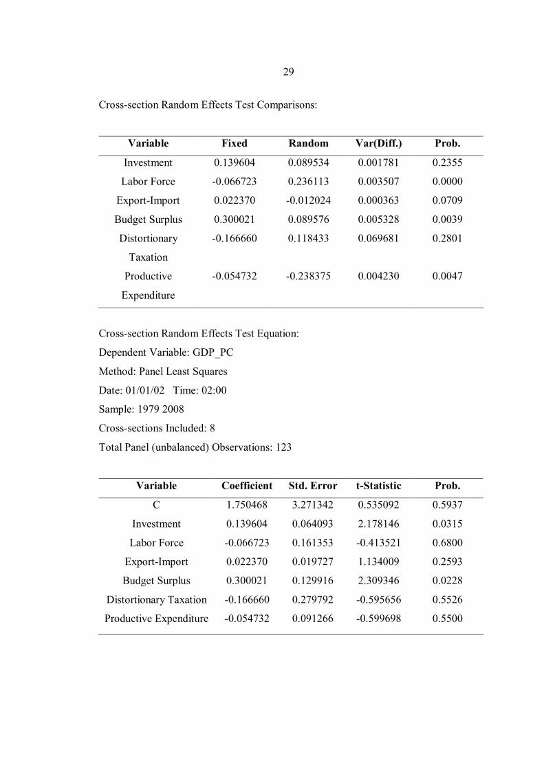
In determining whether to use the fixed effect or random effect model, the

study performs the Hausman Test with the major interested variables (Investment

ratio to GDP, Labor force growth, Export-import ratio to GDP, distortioary taxation,

productive expenditure) and determines that the fixed effect model is the appropriate

model for this empirical study as follows:

Correlated Random Effects - Hausman Test

Equation: EQ01

Test Cross-section Random Effects

Test Summary Chi-Sq.

Statistic

Chi-Sq. d.f.

Prob.

Cross-section random 60.805807 6 0.0000

29

Cross-section Random Effects Test Comparisons:

Variable Fixed Random Var(Diff.) Prob.

Investment 0.139604 0.089534 0.001781 0.2355

Labor Force -0.066723 0.236113 0.003507 0.0000

Export-Import 0.022370 -0.012024 0.000363 0.0709

Budget Surplus 0.300021 0.089576 0.005328 0.0039

Distortionary

Taxation

-0.166660 0.118433 0.069681 0.2801

Productive

Expenditure

-0.054732 -0.238375 0.004230 0.0047

Cross-section Random Effects Test Equation:

Dependent Variable: GDP_PC

Method: Panel Least Squares

Date: 01/01/02 Time: 02:00

Sample: 1979 2008

Cross-sections Included: 8

Total Panel (unbalanced) Observations: 123

Variable Coefficient Std. Error t-Statistic Prob.

C 1.750468 3.271342 0.535092 0.5937

Investment 0.139604 0.064093 2.178146 0.0315

Labor Force -0.066723 0.161353 -0.413521 0.6800

Export-Import 0.022370 0.019727 1.134009 0.2593

Budget Surplus 0.300021 0.129916 2.309346 0.0228

Distortionary Taxation -0.166660 0.279792 -0.595656 0.5526

Productive Expenditure -0.054732 0.091266 -0.599698 0.5500

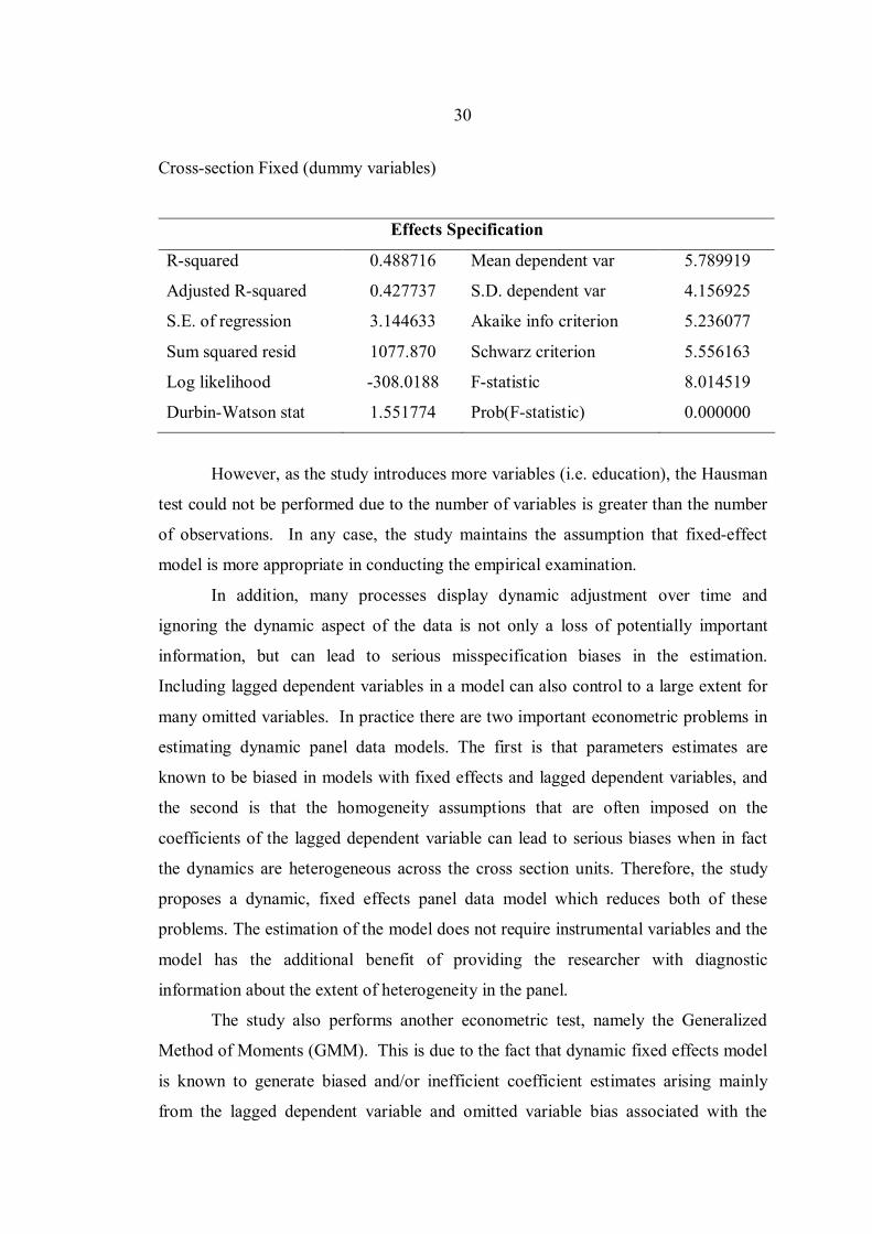
30

Cross-section Fixed (dummy variables)

Effects Specification

R-squared 0.488716 Mean dependent var 5.789919

Adjusted R-squared 0.427737 S.D. dependent var 4.156925

S.E. of regression 3.144633 Akaike info criterion 5.236077

Sum squared resid 1077.870 Schwarz criterion 5.556163

Log likelihood -308.0188 F-statistic 8.014519

Durbin-Watson stat 1.551774 Prob(F-statistic) 0.000000

However, as the study introduces more variables (i.e. education), the Hausman

test could not be performed due to the number of variables is greater than the number

of observations. In any case, the study maintains the assumption that fixed-effect

model is more appropriate in conducting the empirical examination.

In addition, many processes display dynamic adjustment over time and

ignoring the dynamic aspect of the data is not only a loss of potentially important

information, but can lead to serious misspecification biases in the estimation.

Including lagged dependent variables in a model can also control to a large extent for

many omitted variables. In practice there are two important econometric problems in

estimating dynamic panel data models. The first is that parameters estimates are

known to be biased in models with fixed effects and lagged dependent variables, and

the second is that the homogeneity assumptions that are often imposed on the

coefficients of the lagged dependent variable can lead to serious biases when in fact

the dynamics are heterogeneous across the cross section units. Therefore, the study

proposes a dynamic, fixed effects panel data model which reduces both of these

problems. The estimation of the model does not require instrumental variables and the

model has the additional benefit of providing the researcher with diagnostic

information about the extent of heterogeneity in the panel.

The study also performs another econometric test, namely the Generalized

Method of Moments (GMM). This is due to the fact that dynamic fixed effects model

is known to generate biased and/or inefficient coefficient estimates arising mainly

from the lagged dependent variable and omitted variable bias associated with the

31

country-specific effects. These biases typically depend on the characteristics of the

panel (e.g. its time and cross-section dimensions, the exogeneity of the regressors),

which also influences the optimal solution. Following Nickell (1981) and Anderson

and Hsiao (1981), a number of instrumental variable.

Solutions have been proposed to overcome these problems. Recent applications

of these methods to a number of empirical growth models have demonstrated that

they can overturn or substantially modify established results from cross-section or

static panel methods. This paper, therefore, adopts the IV methods under the

Generalized Method of Moments (GMM) to investigate the robustness of fiscal policy

results.

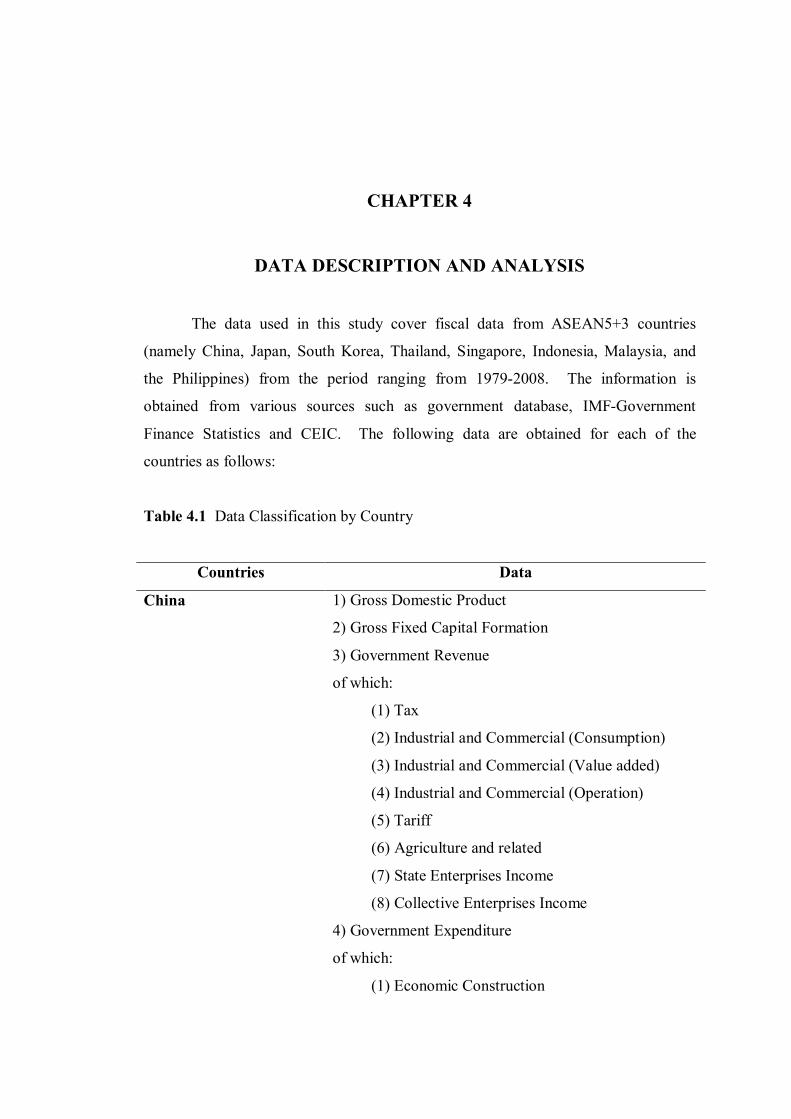
CHAPTER 4

DATA DESCRIPTION AND ANALYSIS

The data used in this study cover fiscal data from ASEAN5+3 countries

(namely China, Japan, South Korea, Thailand, Singapore, Indonesia, Malaysia, and

the Philippines) from the period ranging from 1979-2008. The information is

obtained from various sources such as government database, IMF-Government

Finance Statistics and CEIC. The following data are obtained for each of the

countries as follows:

Table 4.1 Data Classification by Country

Countries Data

China 1) Gross Domestic Product

2) Gross Fixed Capital Formation

3) Government Revenue

of which:

(1) Tax

(2) Industrial and Commercial (Consumption)

(3) Industrial and Commercial (Value added)

(4) Industrial and Commercial (Operation)

(5) Tariff

(6) Agriculture and related

(7) State Enterprises Income

(8) Collective Enterprises Income

4) Government Expenditure

of which:

(1) Economic Construction

33

Table 4.1 (Continued)

Countries Data

(2) Social, Cultural and Education Development

(3) National Defense

(4) Administration

(5) Other Expenses

5) Government Surplus/Deficit

Japan 1) Gross Domestic Product

2) Gross Fixed Capital Formation

3) Government Revenue

of which:

(1) Tax

(2) Social Contribution

(3) Grants

(4) Others

4) Government Expenditure

of which:

(1) Compensation of Employees

(2) Uses of Goods and Services

(3) Consumption of Fixed Capital

(4) Interest

(5) Subsidies

(6) Grants

(7) Social Benefits

(8) Others

5) Government Operating Balance

South Korea 1) Gross Domestic Product

2) Gross Fixed Capital Formation

34

Table 4.1 (Continued)

Countries Data

3) Government Revenue

of which:

(1) Tax

(2) Income, Profits & Capital Gains Tax

(3) Taxes on Property

(4) Customs Duties

(5) Other taxes

(6) Social Security Contributions

(7) Non Tax Revenue

4) Government Expenditure

of which:

(1) Goods and Services

(2) Interest Payments

(3) Subsidies & Other Current Transfers

(4) Acquisition of Capital Assets

(5) Purchases of Capital Stocks

(6) Purchases of Land and Intangible Assets

(7) Capital Transfers

5) Government Balance

Thailand 1) Gross Domestic Product

2) Gross Fixed Capital Formation

3) Government Revenue

of which:

(1) Tax on Income, Profits, and Capital Gain

(2) Social Security Contribution

(3) Tax on Payroll and Workforce

(4) Tax on Property

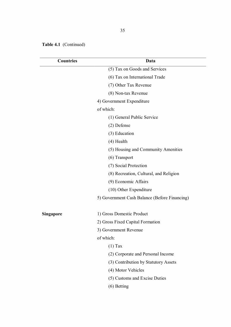
35

Table 4.1 (Continued)

Countries Data

(5) Tax on Goods and Services

(6) Tax on International Trade

(7) Other Tax Revenue

(8) Non-tax Revenue

4) Government Expenditure

of which:

(1) General Public Service

(2) Defense

(3) Education

(4) Health

(5) Housing and Community Amenities

(6) Transport

(7) Social Protection

(8) Recreation, Cultural, and Religion

(9) Economic Affairs

(10) Other Expenditure

5) Government Cash Balance (Before Financing)

Singapore 1) Gross Domestic Product

2) Gross Fixed Capital Formation

3) Government Revenue

of which:

(1) Tax

(2) Corporate and Personal Income

(3) Contribution by Statutory Assets

(4) Motor Vehicles

(5) Customs and Excise Duties

(6) Betting

36

Table 4.1 (Continued)

Countries Data

(7) Stamp Duties

(8) Goods and Services Tax

(9) Other taxes

(10) Fees and Charges

(11) Other Receipts

4) Government Expenditure

of which:

(1) Security and External Relations

(2) Government Administration

(3) Transport

(4) Social Development (SD)

(5) Economic Development (ED)

5) Government Surplus/Deficit

Indonesia 1) Gross Domestic Product

2) Gross Fixed Capital Formation

3) Government Revenue

of which:

(1) Income Tax: Non Oil & Gas

(2) Income Tax Oil & Gas

(3) Value-added Tax

(4) Land & Building Tax

(5) Duties on Land & Building

(6) Excises Duties

(7) International Trade Tax

(8) Other Taxes

(9) Non Taxes

(10) Profit Remittance from SOEs

37

Table 4.1 (Continued)

Countries Data

4) Government Expenditure

of which:

(1) Personnel

(2) Material

(3) Equity

(4) Debt Interest Payment

(5) Subsidies

(6) Grants

(7) Social Services

(8) Other Expenditures

5) Government Balance

Malaysia 1) Gross Domestic Product

2) Gross Fixed Capital Formation

3) Government Revenue

of which:

(1) Income from Companies

(2) Income from Petroleum

(3) Income from Individual

(4) Stamp duty

(5) Other Direct Taxes

(6) Export and Import Duties

(7) Excise Taxes

(8) Sales Taxes

(9) Service Taxes

(10) Other Indirect Taxes

(11) Non-tax Revenues

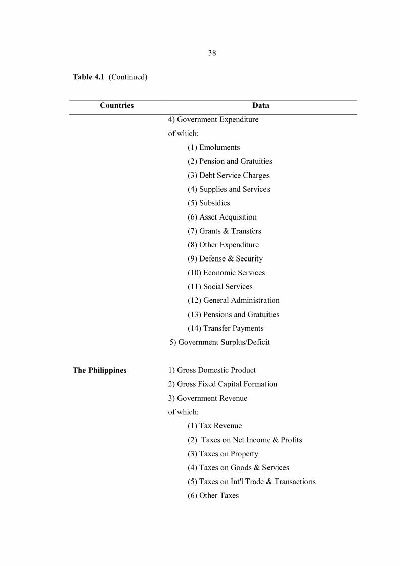
38

Table 4.1 (Continued)

Countries Data

4) Government Expenditure

of which:

(1) Emoluments

(2) Pension and Gratuities

(3) Debt Service Charges

(4) Supplies and Services

(5) Subsidies

(6) Asset Acquisition

(7) Grants & Transfers

(8) Other Expenditure

(9) Defense & Security

(10) Economic Services

(11) Social Services

(12) General Administration

(13) Pensions and Gratuities

(14) Transfer Payments

5) Government Surplus/Deficit

The Philippines 1) Gross Domestic Product

2) Gross Fixed Capital Formation

3) Government Revenue

of which:

(1) Tax Revenue

(2) Taxes on Net Income & Profits

(3) Taxes on Property

(4) Taxes on Goods & Services

(5) Taxes on Int'l Trade & Transactions

(6) Other Taxes

39

Table 4.1 (Continued)

Countries Data

(7) Non Tax Revenue

(8) Collective Enterprises Income

4) Government Expenditure

of which:

(1) Allotment to LGUs

(2) Interest Payments

(3) Tax Expenditures

(4) Subsidy

(5) Other Expenses

5) Government Balance

The theoretical model requires the classification of expenditures into

productive and non-productive and of taxation into distortionary and non-

distortionary. On the expenditure side, the most important component of the non-

productive category is social security. Most other expenditures (i.e. transport and

communication, defense, education, and health) are considered as productive.

Defense spending is considered to be productive expenditure as it is related to the

expenditure to ensure and protect the property rights of the economy.

Based on Bleaney et al. (2001), consumption taxes are classified as non-

distortionary, which is valid if the utility function does not contain leisure as an

argument. With leisure as an argument in the utility function, consumption taxes will

have some impact by distorting the labor-leisure choice. This would leave the category of

non-distortionary taxation as an empty set. Since consumption taxes do not distort the

choice between consumption at different dates, it seems valid to argue that they should

still appear as a different category on the grounds that they are less distortionary than

income taxes. In addition, since the income and substitution effects operate in opposite

directions in the choice between labor and leisure, the impact of consumption taxation

on labor input may, in practice, be small. Whether they are non-distortionary or

merely less distortionary than other taxes is a question that can be answered in the

40

empirical estimation. Finally, there are some revenues and expenditures whose

classification is ambiguous and are labeled as ‘other revenues’ and ‘other expenditures.’

The categorization of government taxes and expenditures are as follows:

Table 4.2 Fiscal Data Classifications

Theoretical Classifications Functional Classifications

Budget surplus Budget surplus

Distortionary taxation Taxation on income and profit

Social Security Contributions

Taxation on payroll and manpower

Taxation on property

Non-distortionary taxation Taxation on domestic goods and services

Other revenues Taxation on international trade

Non-tax revenues

Other tax revenues

Productive expenditures General public services expenditure

Educational expenditure

Health Expenditure

Housing Expenditure

Transport and communication expenditure

Non-productive expenditures Social security and welfare expenditure

Expenditure on recreation

Expenditure on economic services

Defense expenditure

Other expenditures Other expenditure (unclassified)

Based on endogenous growth theory, distortionary taxation is expected to have

a large negative effect on growth, while productive expenditure is expected to have

significant positive coefficient. Budget balance is expected to have positive effect on

growth as the surplus is constrained to finance the neutral elements of the budget,

which have no growth effects, whereas the compensating future deficits anticipated

41

under Ricardian equivalence may partially finance productive expenditure or cuts in

distortionary taxation, raising the anticipated returns to investment and hence growth.

The dependent variable is per capita GDP growth. The independent variables

are classified as fiscal variables and non-fiscal variables.

Fiscal variables are:

1) Distortionary taxation to GDP

2) Non-distortionary taxation to GDP

3) Other revenues to GDP

4) Productive expenditure to GDP

5) Non-productive expenditure to GDP

6) Other expenditure to GDP

7) Budget surplus to GDP

Non-fiscal variables are:

1) Domestic investment to GDP

2) Labor force growth

3) Export-import to GDP (proxy for trade openness)

4) School enrollment ratio (proxy for human capital)

5) Dummy variable for 1997 Asian financial crisis

Before focusing on the results, it is worthwhile to provide a quick summary of

the explanatory variables as follows:

1) Distortionary Taxation – ASEAN5+3 countries have the mean distortionary

tax at 10.0 percent of GDP with the maximum mean value at 19.7 percent of GDP

(Malaysia) and the minimum mean value at 5.9 percent of GDP (the Philippines).

Distortionary taxes in Malaysia are mostly income-based taxes imposed on

corporations (45.9 percent of income-based tax in 2009) and petroleum industry (29.4

percent of income-based tax in 2009), while individuals pay a lesser share (18.2

percent of income-based tax in 2009). The Philippines has the lowest level of

distortionary tax at 5.9 percent of GDP compared to other ASEAN5+3 countries.

Nonetheless, over the period from 1990-2008, the Philippines had been increasing its

share of income-based tax revenue from 32.5 percent of total tax revenue in 1990 to

45.9 percent of total tax revenue in 2008. Overall, in most countries, except for the

Philippines and Thailand, distortionary taxation to GDP generates substantial share of

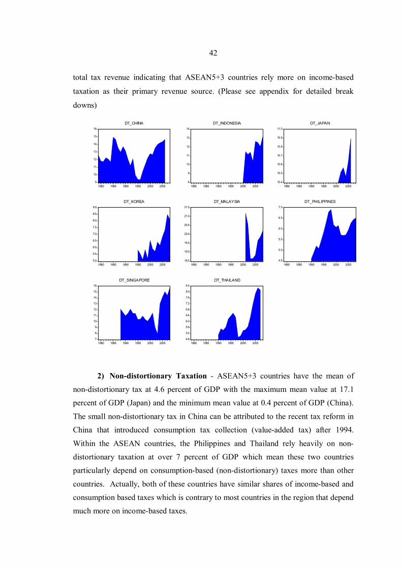
42

total tax revenue indicating that ASEAN5+3 countries rely more on income-based

taxation as their primary revenue source. (Please see appendix for detailed break

downs)

9

10

11

12

13

14

15

16

1980 1985 1990 1995 2000 2005

DT_CHINA

8

9

10

11

12

13

14

1980 1985 1990 1995 2000 2005

DT_INDONESIA

10.4

10.5

10.6

10.7

10.8

10.9

11.0

1980 1985 1990 1995 2000 2005

DT_JAPAN

5.0

5.5

6.0

6.5

7.0

7.5

8.0

8.5

9.0

1980 1985 1990 1995 2000 2005

DT_KOREA

18.5

19.0

19.5

20.0

20.5

21.0

21.5

1980 1985 1990 1995 2000 2005

DT_MALAYSIA

4.5

5.0

5.5

6.0

6.5

7.0

1980 1985 1990 1995 2000 2005

DT_PHILIPPINES

7

8

9

10

11

12

13

14

15

16

1980 1985 1990 1995 2000 2005

DT_SINGAPORE

4.8

5.2

5.6

6.0

6.4

6.8

7.2

7.6

8.0

8.4

1980 1985 1990 1995 2000 2005

DT_THAILAND

2) Non-distortionary Taxation - ASEAN5+3 countries have the mean of

non-distortionary tax at 4.6 percent of GDP with the maximum mean value at 17.1

percent of GDP (Japan) and the minimum mean value at 0.4 percent of GDP (China).

The small non-distortionary tax in China can be attributed to the recent tax reform in

China that introduced consumption tax collection (value-added tax) after 1994.

Within the ASEAN countries, the Philippines and Thailand rely heavily on non-

distortionary taxation at over 7 percent of GDP which mean these two countries

particularly depend on consumption-based (non-distortionary) taxes more than other

countries. Actually, both of these countries have similar shares of income-based and

consumption based taxes which is contrary to most countries in the region that depend

much more on income-based taxes.

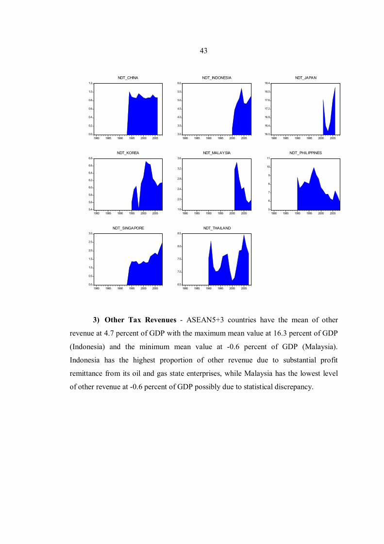
43

0.0

0.2

0.4

0.6

0.8

1.0

1.2

1980 1985 1990 1995 2000 2005

NDT_CHINA

3.0

3.5

4.0

4.5

5.0

5.5

6.0

1980 1985 1990 1995 2000 2005

NDT_INDONESIA

16.0

16.4

16.8

17.2

17.6

18.0

18.4

1980 1985 1990 1995 2000 2005

NDT_JAPAN

5.4

5.6

5.8

6.0

6.2

6.4

6.6

6.8

1980 1985 1990 1995 2000 2005

NDT_KOREA

1.6

2.0

2.4

2.8

3.2

3.6

1980 1985 1990 1995 2000 2005

NDT_MALAYSIA

5

6

7

8

9

10

11

1980 1985 1990 1995 2000 2005

NDT_PHILIPPINES

0.0

0.5

1.0

1.5

2.0

2.5

3.0

1980 1985 1990 1995 2000 2005

NDT_SINGAPORE

6.5

7.0

7.5

8.0

8.5

1980 1985 1990 1995 2000 2005

NDT_THAILAND

3) Other Tax Revenues - ASEAN5+3 countries have the mean of other

revenue at 4.7 percent of GDP with the maximum mean value at 16.3 percent of GDP

(Indonesia) and the minimum mean value at -0.6 percent of GDP (Malaysia).

Indonesia has the highest proportion of other revenue due to substantial profit

remittance from its oil and gas state enterprises, while Malaysia has the lowest level

of other revenue at -0.6 percent of GDP possibly due to statistical discrepancy.

44

-2

0

2

4

6

8

1980 1985 1990 1995 2000 2005

OR_CHINA

11

12

13

14

15

16

17

18

19

1980 1985 1990 1995 2000 2005

OR_INDONESIA

3.0

3.5

4.0

4.5

5.0

5.5

6.0

6.5

1980 1985 1990 1995 2000 2005

OR_JAPAN

6

7

8

9

10

11

1980 1985 1990 1995 2000 2005

OR_KOREA

-2.4

-2.0

-1.6

-1.2

-0.8

-0.4

0.0

0.4

0.8

1980 1985 1990 1995 2000 2005

OR_MALAYSIA

1

2

3

4

5

6

7

1980 1985 1990 1995 2000 2005

OR_PHILIPPINES

-4

-2

0

2

4

6

8

10

1980 1985 1990 1995 2000 2005

OR_SINGAPORE

3.5

4.0

4.5

5.0

5.5

6.0

6.5

1980 1985 1990 1995 2000 2005

OR_THAILAND

4) Productive Expenditure - ASEAN5+3 countries have the mean of

productive expenditure at 8.9 percent of GDP with the maximum mean value at 13.9

percent of GDP (Malaysia) and the minimum mean value at 2.8 percent of GDP

(Indonesia). Malaysia has the highest proportion of productive expenditure at 13.9

percent of GDP as most of the government spending are for government wages &

salary and development projects (82 percent of total government spending in 2008)

and smaller amount for social services (18 percent of total government spending in

2008). Indonesia has the lowest level of productive expenditure due to relatively

small size of capital spending relatively to large oil and gas subsidy and interest

payment (non-productive expenditures).

45

4

8

12

16

20

24

28

1980 1985 1990 1995 2000 2005

PEX_CHINA

0

1

2

3

4

5

6

1980 1985 1990 1995 2000 2005

PEX_INDONESIA

12.5

12.6

12.7

12.8

12.9

13.0

13.1

1980 1985 1990 1995 2000 2005

PEX_JAPAN

6.8

7.2

7.6

8.0

8.4

8.8

1980 1985 1990 1995 2000 2005

PEX_KOREA

11

12

13

14

15

16

17

18

19

1980 1985 1990 1995 2000 2005

PEX_MALAYSIA

0.5

1.0

1.5

2.0

2.5

3.0

3.5

4.0

1980 1985 1990 1995 2000 2005

PEX_PHILIPPINES

0

4

8

12

16

20

1980 1985 1990 1995 2000 2005

PEX_SINGAPORE

8

9

10

11

12

13

1980 1985 1990 1995 2000 2005

PEX_THAILAND

5) Non-productive Expenditure - ASEAN5+3 countries have the mean of

non-productive expenditure at 6.0 percent of GDP with the maximum mean value at

20.8 percent of GDP (Japan) and the minimum mean value at 1.4 percent of GDP

(Thailand). Japan has the highest proportion of non-productive expenditure at 20.8

percent of GDP because it has large social benefit expenditure comprising almost 50

percent of the total government expenditure, while Thailand has the lowest level of

non-productive expenditure at 1.4 percent of GDP as it has relatively lower 1) social

protection and 2) recreation, culture, religion expenditure at 5.7 percent and 1.6

percent of the total government expenditure, respectively throughout 1990s However,

it is important to note that social protection expenditure has been increasing

dramatically after 2000 to averaging 18.5 percent of the total government expenditure

during the period between 2000-2007.

46

2.8

3.2

3.6

4.0

4.4

4.8

5.2

1980 1985 1990 1995 2000 2005

NPEX_CHINA

0

1

2

3

4

5

6

7

1980 1985 1990 1995 2000 2005

NPEX_INDONESIA

20.5

20.6

20.7

20.8

20.9

21.0

21.1

1980 1985 1990 1995 2000 2005

NPEX_JAPAN

12

14

16

18

20

22

24

26

1980 1985 1990 1995 2000 2005

NPEX_KOREA

12

14

16

18

20

22

24

26

28

1980 1985 1990 1995 2000 2005

NPEX_MALAYSIA

3

4

5

6

7

8

1980 1985 1990 1995 2000 2005

NPEX_PHILIPPINES

0

1

2

3

4

5

6

1980 1985 1990 1995 2000 2005

NPEX_SINGAPORE

0.4

0.8

1.2

1.6

2.0

2.4

2.8

1980 1985 1990 1995 2000 2005

NPEX_THAILAND

6) Other Expenditures - ASEAN5+3 countries have the mean of other

expenditure at 10.0 percent of GDP with the maximum mean value at 19.3 percent of

GDP (Korea) and the minimum mean value at 0.4 percent of GDP (Malaysia).

47

8

12

16

20

24

28

32

1980 1985 1990 1995 2000 2005

OEX_CHINA

4

8

12

16

20

24

28

32

36

1980 1985 1990 1995 2000 2005

OEX_INDONESIA

1.9

2.0

2.1

2.2

2.3

2.4

1980 1985 1990 1995 2000 2005

OEX_JAPAN

15

16

17

18

19

20

21

22

23

1980 1985 1990 1995 2000 2005

OEX_KOREA

0.0

0.2

0.4

0.6

0.8

1.0

1.2

1980 1985 1990 1995 2000 2005

OEX_MALAYSIA

8

9

10

11

12

13

1980 1985 1990 1995 2000 2005

OEX_PHILIPPINES

-8

-4

0

4

8

12

16

1980 1985 1990 1995 2000 2005

OEX_SINGAPORE

-1

0

1

2

3

4

5

6

7

8

1980 1985 1990 1995 2000 2005

OEX_THAILAND

7) Budget Surplus - ASEAN5+3 countries have the mean of budget deficit

at -0.05 percent of GDP with the maximum mean value at 8.9 percent of GDP

(Singapore) and the minimum mean value at -4.0 percents of GDP (Japan). Singapore

has the highest ratio of budget surplus. In the case of Singapore, the fiscal position

has been aided by strong economic growth so that the Singapore government has been

able to keep both the tax rate and the government expenditure rate low and yet

generate healthy budget surpluses year after year. Although the gap between the tax

rate and the government expenditure rate is the obvious source of the surplus, another

subtle source of fiscal surplus is generated by conservative growth forecasts that lay

the base for revenue projections. On average the under-prediction of the tax base

(GDP) must have contributed about 13 percent per year to the realized budget surplus

over the period 1990–2005. This appears to be simply a by-product of the

48

Government’s philosophy of ‘‘fiscal prudence’’. In the case of Japan, sustained fiscal

deficits in recent years have been the norm to stimulate the slacking domestic

economy. Japan budget deficit grew during the 1990s. After the bubble economy

collapsed, the budget balance of Japan has been declining at significant rate.

-4

-3

-2

-1

0

1

1980 1985 1990 1995 2000 2005

BS_CHINA

-5

-4

-3

-2

-1

0

1980 1985 1990 1995 2000 2005

BS_INDONESIA

-6

-5

-4

-3

-2

-1

0

1980 1985 1990 1995 2000 2005

BS_JAPAN

-4

-3

-2

-1

0

1

2

3

4

1980 1985 1990 1995 2000 2005

BS_KOREA

-6

-4

-2

0

2

4

1980 1985 1990 1995 2000 2005

BS_MALAYSIA

-6

-5

-4

-3

-2

-1

0

1

2

1980 1985 1990 1995 2000 2005

BS_PHILIPPINES

-4

0

4

8

12

16

20

1980 1985 1990 1995 2000 2005

BS_SINGAPORE

-4

-3

-2

-1

0

1

2

3

1980 1985 1990 1995 2000 2005

BS_THAILAND

8) Domestic Investment - ASEAN5+3 countries have the mean of domestic

investment at 26.9 percent of GDP with the maximum mean value at 32.1 percent of

GDP (China) and the minimum mean value at 19.4 percent of GDP (the Philippines).

China has very high investment ratio attributed to both high level of domestic saving

as well as large influx of foreign direct investment into the country. In the Philippines,

there are 3 main reasons for low domestic investment: 1) the public sector is

constrained by serious fiscal pressures, due to decades of weak revenue performance

(i.e. not enough tax-money to cover the expenditures) and a weighty debt service.

Hence, it cannot keep public investment growing at GDP growth rates 2) the capital-

intensive private sector does not find it convenient - as it expects little returns on each

49

dollar it spends - to expand investment relative to economic growth as the public

sector does not invest enough to provide incentives for private investment. If there is

no road, and the supply of electricity is spotty, why should you invest to open a

business? In addition, Élite-capture in the traditional sectors of the economy. Assume

you are part of the local élite; your company enjoys favorable rules and regulations -

and is allowed to charge high prices; if this happens in a systemic way, this protection

reduces other companies’ incentives to invest. In the Philippines, inputs are expensive

because a few politically-connected corporate conglomerates enjoy barriers to entry

and oligopolistic market power, and sell at a high price the products (agricultural

commodities, transport services, electricity, cement, etc.) that are critical for the

economy. Also, with their rents these conglomerates pay higher wages - relative to

other Asian countries - to the salaried insiders, thus securing “national labor peace”

3) The fast-growing businesses in the service sector in the Philippines - electronics

assembly, voice-based business process outsourcing, and information technology - do

not need to increase their investment at GDP growth rates to enjoy fast-rising profits.

It is the nature of the business: it needs little capital and lots of skilled labor.

50

24

28

32

36

40

44

1980 1985 1990 1995 2000 2005

INV_CHINA

19

20

21

22

23

24

1980 1985 1990 1995 2000 2005

INV_INDONESIA

22.8

23.2

23.6

24.0

24.4

24.8

1980 1985 1990 1995 2000 2005

INV_JAPAN

26

28

30

32

34

36

38

40

1980 1985 1990 1995 2000 2005

INV_KOREA

20

21

22

23

24

25

1980 1985 1990 1995 2000 2005

INV_MALAYSIA

12

14

16

18

20

22

24

26

1980 1985 1990 1995 2000 2005

INV_PHILIPPINES

20

24

28

32

36

40

1980 1985 1990 1995 2000 2005

INV_SINGAPORE

16

20

24

28

32

36

40

44

1980 1985 1990 1995 2000 2005

INV_THAILAND

9) Export-import – ASEAN5+3 countries have the mean of export-import at

97.3 percent of GDP with the maximum mean value at 296.7 percent of GDP

(Singapore) and the minimum mean value at 22.2 percent of GDP (Japan).

51

10

20

30

40

50

60

70

1980 1985 1990 1995 2000 2005

EXIM_CHINA

44

48

52

56

60

64

68

72

76

1980 1985 1990 1995 2000 2005

EXIM_INDONESIA

18

20

22

24

26

28

30

1980 1985 1990 1995 2000 2005

EXIM_JAPAN

50

60

70

80

90

100

110

1980 1985 1990 1995 2000 2005

EXIM_KOREA

120

124

128

132

136

140

144

148

1980 1985 1990 1995 2000 2005

EXIM_MALAYSIA

40

50

60

70

80

90

100

110

120

1980 1985 1990 1995 2000 2005

EXIM_PHILIPPINES

240

260

280

300

320

340

360

1980 1985 1990 1995 2000 2005

EXIM_SINGAPORE

60

70

80

90

100

110

120

130

140

1980 1985 1990 1995 2000 2005

EXIM_THAILAND

10) Educational Attainment In this study, educational attainment is represented

by school enrollment both at the secondary and tertiary levels as follows:

(1) Secondary school enrollment ratio - ASEAN5+3 countries have

the mean of secondary school enrollment ratio at 70.9 percent with the maximum

mean value at 101.1 percent (Japan) and the minimum mean value at 49.5 percent

(Singapore).

52

35

40

45

50

55

60

65

70

75

1980 1985 1990 1995 2000 2005

EDUSEC_CHINA

56

60

64

68

72

76

1980 1985 1990 1995 2000 2005

EDUSEC_INDONESIA

100.6

100.8

101.0

101.2

101.4

101.6

101.8

102.0

1980 1985 1990 1995 2000 2005

EDUSEC_JAPAN

92

96

100

104

108

1980 1985 1990 1995 2000 2005

EDUSEC_KOREA

65

66

67

68

69

70

71

72

73

1980 1985 1990 1995 2000 2005

EDUSEC_MALAYSIA

70

72

74

76

78

80

82

84

1980 1985 1990 1995 2000 2005

EDUSEC_PHILIPPINES

30

40

50

60

70

80

1980 1985 1990 1995 2000 2005

EDUSEC_SINGAPORE

20

30

40

50

60

70

80

1980 1985 1990 1995 2000 2005

EDUSEC_THAILAND

(2) Tertiary school enrollment ratio - ASEAN5+3 countries have the

mean of tertiary school enrollment ratio at 35.8 percent with the maximum value at

79.3 percent (Korea) and the minimum value at 6.0 percent (China).

53

0

4

8

12

16

20

24

1980 1985 1990 1995 2000 2005

EDUTER_CHINA

13

14

15

16

17

18

19

20

21

22

1980 1985 1990 1995 2000 2005

EDUTER_INDONESIA

50

51

52

53

54

55

56

57

58

1980 1985 1990 1995 2000 2005

EDUTER_JAPAN

40

50

60

70

80

90

100

1980 1985 1990 1995 2000 2005

EDUTER_KOREA

25

26

27

28

29

30

31

32

33

1980 1985 1990 1995 2000 2005

EDUTER_MALAYSIA

24

25

26

27

28

29

30

31

1980 1985 1990 1995 2000 2005

EDUTER_PHILIPPINES

20

30

40

50

60

70

1980 1985 1990 1995 2000 2005

EDUTER_SINGAPORE

15

20

25

30

35

40

45

50

1980 1985 1990 1995 2000 2005

EDUTER_THAILAND

11) GDP Per Capita - ASEAN5+3 countries have the mean of GDP per

capita growth at 4.8 percent with the maximum mean value at 9.3 percent of GDP (the

Philippines) and the minimum mean value at -0.5 percent of GDP (Japan).

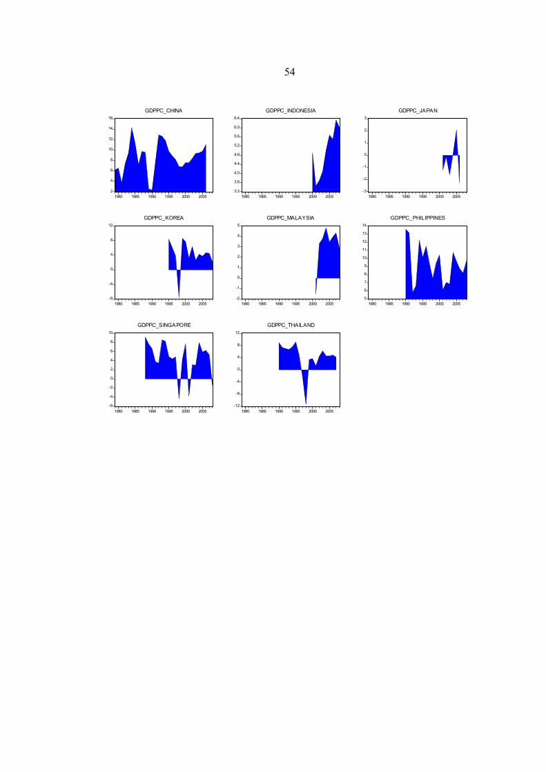
54

2

4

6

8

10

12

14

16

1980 1985 1990 1995 2000 2005

GDPPC_CHINA

3.2

3.6

4.0

4.4

4.8

5.2

5.6

6.0

6.4

1980 1985 1990 1995 2000 2005

GDPPC_INDONESIA

-3

-2

-1

0

1

2

3

1980 1985 1990 1995 2000 2005

GDPPC_JAPAN

-8

-4

0

4

8

12

1980 1985 1990 1995 2000 2005

GDPPC_KOREA

-2

-1

0

1

2

3

4

5

1980 1985 1990 1995 2000 2005

GDPPC_MALAYSIA

5

6

7

8

9

10

11

12

13

14

1980 1985 1990 1995 2000 2005

GDPPC_PHILIPPINES

-6

-4

-2

0

2

4

6

8

10

1980 1985 1990 1995 2000 2005

GDPPC_SINGAPORE

-12

-8

-4

0

4

8

12

1980 1985 1990 1995 2000 2005

GDPPC_THAILAND

CHAPTER 5

EMPIRICAL RESULTS

The empirical results are shown for ASEAN5+3 and ASEAN5 to analyze the

determining factors for growth with per capita GDP growth as the dependent variable.

As mentioned before, the methodologies used in this study are 1) dynamic fixed-

effect model and 2) generalized method of moments (GMM) model.

For the ASEAN5+3 countries, the empirical results for the fiscal variables are

consistent with endogenous growth theory that distortionary taxation has negative

effect, while productive expenditure has positive effect on growth. Non-distortionary

taxation and non-productive expenditure have no statistically-significant on growth.

Budget surplus (indicating fiscal discipline) shows positive impact on growth as well

which is consistent with the predictions of Barro and Sala-i-Martin (1992) model. In

addition, for non-fiscal variable, investment ratio to GDP and export-import ratio to

GDP (proxy for trade openness) show significant positive impact on growth.

Interestingly, secondary education as represented by its enrollment ratio shows no

statistical significant to growth, while tertiary education as represented by its

enrollment ratio shows positive impact on growth. However, on the educational

variables, previous studies have shown inconclusive results on their impact on growth.

Krueger and Lindahl (2001) has suggested that this may be largely due to the

reliability of country-level data that may be due to measurement errors and

incomplete data.

The empirical results for ASEAN5+3 are presented in Table 2.3 as follows:

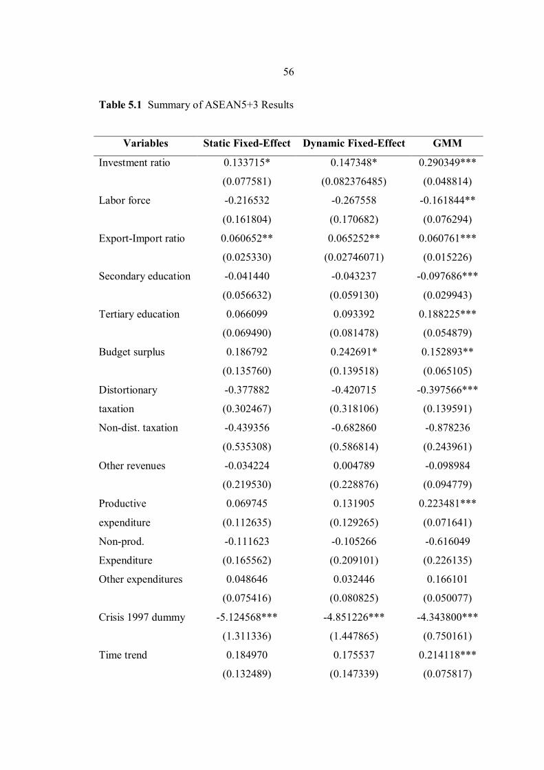
56

Table 5.1 Summary of ASEAN5+3 Results

Variables Static Fixed-Effect Dynamic Fixed-Effect GMM

Investment ratio 0.133715* 0.147348* 0.290349***

(0.077581) (0.082376485) (0.048814)

Labor force -0.216532

(0.161804)

-0.267558

(0.170682)

-0.161844**

(0.076294)

Export-Import ratio 0.060652**

(0.025330)

0.065252**

(0.02746071)

0.060761***

(0.015226)

Secondary education -0.041440

(0.056632)

-0.043237

(0.059130)

-0.097686***

(0.029943)

Tertiary education 0.066099

(0.069490)

0.093392

(0.081478)

0.188225***

(0.054879)

Budget surplus 0.186792

(0.135760)

0.242691*

(0.139518)

0.152893**

(0.065105)

Distortionary

taxation

-0.377882

(0.302467)

-0.420715

(0.318106)

-0.397566***

(0.139591)

Non-dist. taxation -0.439356

(0.535308)

-0.682860

(0.586814)

-0.878236

(0.243961)

Other revenues -0.034224

(0.219530)

0.004789

(0.228876)

-0.098984

(0.094779)

Productive

expenditure

0.069745

(0.112635)

0.131905

(0.129265)

0.223481***

(0.071641)

Non-prod.

Expenditure

-0.111623

(0.165562)

-0.105266

(0.209101)

-0.616049

(0.226135)

Other expenditures 0.048646

(0.075416)

0.032446

(0.080825)

0.166101

(0.050077)

Crisis 1997 dummy -5.124568***

(1.311336)

-4.851226***

(1.447865)

-4.343800***

(0.750161)

Time trend 0.184970

(0.132489)

0.175537

(0.147339)

0.214118***

(0.075817)

57

Table 5.1 (Continued)

Variables Static Fixed-Effect Dynamic Fixed-Effect GMM

Lagged growth -

-0.021469

(0.111611)

-0.030991

(0.064046)

Constant term 1.703962

(4.703481)

1.157686

(5.020937)

-

Note: 1. *** denotes statistical significance at 1% confidence level

** denotes statistical significance at 5% confidence level

* denotes statistical significance at 10% confidence level

2. Standard errors are shown in parentheses.

For the ASEAN5 countries, the empirical results for the fiscal variables are

not consistent with endogenous growth theory as distortionary taxation and productive

expenditure has no statically significant impact on growth. Interestingly, non-

productive expenditure show statistically-significant positive impact on growth. Like

in the case of ASEAN5+3, budget surplus (indicating fiscal discipline) shows quite

strong positive impact on growth for ASEAN5 which is also consistent with economic

theory. For non-fiscal variable, investment ratio to GDP and export-import ratio to

GDP (proxy for trade openness) show significant positive impact on growth which is

similar to the case of ASEAN5+3. Labor force is shown to have statically-significant

negative impact on growth. Interestingly, secondary education as represented by its

enrollment ratio shows statistically-significant negative impact on growth for

ASEAN5 countries, while tertiary education as represented by its enrollment ratio

shows no statically-significant impact on growth.

The empirical results for ASEAN5 are presented in Table 2 as follows:

58

Table 5.2 Summary of ASEAN5 Results

Variables Static

Fixed-Effect

Dynamic

Fixed-Effect

GMM

Investment ratio -0.096693

(0.113386) -0.061393

(0.124841) 0.028960

(0.062175) Labor force -0.021987

(0.265243)

-0.097450

(0.300196)

-0.283022***

(0.104457)

Export-Import ratio 0.104784***

(0.030655)

0.116771***

(0.035238)

0.127414***

(0.012010)

Secondary education -0.210822**

(0.082507)

-0.235081**

(0.090532)

-0.182520***

(0.035647)

Tertiary education -0.055142

(0.123105)

-0.029488

(0.142674)

-0.088545

(0.056974)

Budget surplus 0.367128**

(0.146417)

0.370075**

(0.152536)

0.351281***

(0.081809)

Distortionary taxation -0.069095

(0.472173)

0.100082

(0.584315)

-0.206669

(0.303492)

Non-dist. taxation -0.102475

(0.697350)

-0.243323

(0.784268)

0.044507

(0.418863)

Other revenues 0.263638

(0.239556)

0.294839

(0.300670)

0.104287

(0.229229)

Productive expenditure -0.299577

(0.227699)

-0.265003

(0.276853)

-0.474824

(0.424557)

Non-prod. Expenditure 1.141915***

(0.389598)

1.102947**

(0.489052)

1.511662***

(0.278243)

Other expenditures -0.099880*

(0.051278) -0.084638

(0.068593) -0.100915**

(0.052889) Crisis 1997 dummy -5.934828***

(1.862713) -6.747437***

(2.005283) -7.195227**

(1.890931) Time trend 0.323448

(0.212293) 0.352909

(0.226792) 0.351433**

(0.141078) Lagged growth - -0.187472

(0.155257) -0.333784***

(0.079785)

59

Table 5.2 (Continued)

Variables Static

Fixed-Effect

Dynamic

Fixed-Effect

GMM

Prod. expenditure 1997 - -

-0.102867

(0.435391) Constant term 2.979965

(6.613625) 0.668304

(7.835436) -

Note: 1. *** denotes statistical significance at 1% confidence level

** denotes statistical significance at 5% confidence level

* denotes statistical significance at 10% confidence level

2. Standard errors are shown in parentheses.

Conclusion and Policy Recommendations

This study attempts to identify the role of fiscal policy in promoting economic

progress using the panel data for the five ASEAN countries (Thailand, Singapore,

Indonesia, Malaysia and the Philippines) and the Plus Three countries (China, Japan,

and Republic of Korea). This study classifies fiscal policy into productive versus

non-productive expenditure and distortionary versus non-distortionary taxation to

examine in details how fiscal policy implemented by ASEAN5+3 countries has

impacted growth. Other non-fiscal variables are also included such as domestic

investment, international trade, and labor force. The overall results strongly suggest

that fiscal policy in the ASEAN5+3 does have discernable impact to explain the

strong growth performances in the region. Distortionary taxation is shown to have

negative long-run effect on growth, while productive expenditures show positive

long-run effect on growth. Budget surplus, an indicator for fiscal prudence, also

shows positive relationship with economic performance. Obviously, it should be

noted with caution that the effectiveness of fiscal policy is certainly not just the

amount of expenditures, but other “intangible” such as fiscal institutions and

corruption may also affect fiscal policy impact on the economy as well. On the non-

60

fiscal aspect, economic growth can also be attributed to higher domestic investment,

international trade, and prudent fiscal policy as the underlying factors in supporting

growth in the past decades. These findings are mostly consistent with Bleaney et al.

(2001) for OECD countries where productive expenditure and distortionary taxation

also show positive and negative effects on growth, respectively.

Based on the empirical results, the following conclusion and policy

recommendations can be made:

1) Taxation and public expenditures have long-term implications on

economic growth in ASEAN5+3 countries. This is consistent with the view of the

endogenous growth model which states that fiscal policy can have long-term effect on

economic growth.

2) Consistent with theoretical predictions, distortionary tax has negative

impact while productive expenditure has positive impact on growth in the region. Tax

can generate negative impact on economic growth in which the government must

consider the costs and benefits of implementing specific tax policies in order to

minimize economic distortions and to ensure that the negative effect from rising the

fiscal resources would be offset by the positive effect after the fiscal resources are

deployed through spending policies. Negative impact of tax is the “social cost” of

public policy – therefore, optimal tax policy to minimize distortion is crucial.

Therefore, government should focus on delivering tax strategies that would minimize

negative growth impact.

3) Over the longer term, the government should seek to lower the income-

based tax burden and increase the consumption-based tax burden which would lessen

work incentive distortion, promote saving and capital formation in the economy.

4) Prudent fiscal policy is crucial to economic growth. Excessive fiscal

deficits can lead to crowding out of private investment, higher interest rate, and real

exchange rate appreciation which all would worsen competitiveness. Based on the

statistical data, countries with prudential fiscal policy are associated with higher

growth rate per capita particularly for Singapore and South Korea. It is important for

policy-makers to aim at anchoring medium-term fiscal credibility through the uses of

appropriate framework for “fiscal rules.” In recent years, many countries have

renewed efforts to strengthen fiscal frameworks, in particular, fiscal rules and

61

budgetary frameworks. Although rules cannot substitute for long-term resolve to

implement prudent fiscal policies, they can strengthen the credibility of policymakers

and anchor near-term policies to avoid dangerous currents that may otherwise be

difficult to resist.

5) Countries should focus their policies to promote investment and trade

openness. Domestic investment enhances productivity which in turn spurs long-term

economic growth. Countries with relatively high domestic investment to GDP have

shown relatively higher income per capita growth such as China, South Korea, and

Singapore. International trade openness also fosters growth as openness to imports

increases efficiency and reduces costs for industry. Exposure to foreign competition

forces domestic industry to become more efficient and competitive. It also aids this

process by reducing the cost of key foreign inputs and enabling access to cost-saving

and quality enhancing new technologies. In addition, openness to imports reduces

costs and increases quantity demanded for consumers. In the end, it is almost always

the consumers who pay the price of protectionism through lower quality goods and

higher prices. Reducing trade barriers brings greater variety of products and quality,

but also lower prices. This welfare effect for consumers is often the strongest element

in the impact of liberalization, particularly for highly protected industries.

6) ASEAN5 countries are especially vulnerable to external shocks (i.e. 1997

financial crisis) so policy-makers need to continually strengthen economic resiliency

and immunity in the region.

Overall, this study suggests that the role of public sector and fiscal policy in

ASEAN5+3 should be carefully analyzed as it has strong potentials to affect growth

performances either positively and negatively with the aim to achieve better growth

results in the coming years.

62

BIBLIOGRAPHY

Abdi, Tahir A. 2004. Machinery & Equipment Investment and Growth:

Evidence from the Canadian Manufacturing Sector. Working Paper. 4.

Canada: Department of Finance Canada.

Abeysinghe, Tilak and Jayawickrama, Ananda. 2008. Singapore’s Recurrent Budget

Surplus: The Role of Conservative Growth Forecasts. Journal of Asian

Economics. 19: 117–124.

Abu-Bader, Suleiman and Abu-Qarn, Aamer. 2003. Government Expenditures,

Military Spending and Economic Growth:Causality Evidence from

Egypt, Israel and Syria Department of Economics. Beer-Sheva, Israel:

Ben-Gurion University of the Negev.

Acemoglu, Daron; Johnson, Simon and Robinson, James A. 2001. The Colonial

Origins of Comparative Development: An Empirical Investigation.

American Economic Review. 91 (5): 1369-1401.

Adam, Christopher S. and Bevan, David L. 2005. Fiscal Deficits and Growth in

Developing Countries. Journal of Public Economics. 89: 571-597.

Aghion, P. and Howitt, P. 1992. A Model of Growth through Creative Destruction.

Econometrica. 60: 323-351.

Aisen, Ari. 2007. Growth Determinants in Low-Income and Emerging Asia: A

Comparative Analysis. Asia-Pacific Development Journal. 14, 2

(December): 1-22.

Anderson, T. W. and Hsiao, C. 1981. Estimation of Dynamic Models with Error

Components. Journal of the American Statistical Association. 76: 598-

606.

Atkinson, Anthony B. 1995. The Welfare State and Economic Performance.

National Tax Journal. 48, 2 (June): 171–198.

Bagdigen, Muhilis and Cetintas, Hakan. Causality between Public Expenditure and

Economic Growth: The Turkish Case. Journal of Economic and Social

Research. 6 (1): 53-72.

63

Ball, Laurence and Mankiw, N. Gregory. 1995. What Do Budget Deficits Do? In

Budget Deficits and Debt: Issues and Options. Kansas City: Federal

Reserve Bank of Kansas City. Pp.95-119.

Barro, Robert J. 1990. Government Spending in a Simple Model of Endogenous

Growth. Journal of Political Economy. 98 (5): 103-125.

Barro, Robert J. 1991a. A Cross-Country Study of Growth, Saving, and

Government. Chicago: University of Chicago Press and NBER.

Barro, Robert J. 1991b. Economic Growth in a Cross-Section of Countries.

Quarterly Journal of Economics. 104 (May): 407-444.

Barro, Robert J. 1997. Determinants of Economic Growth: A Cross-Country

Empirical Study. Cambridge, MA.: MIT Press.

Barro, Robert J. and Lee, Jong Wha. 1993. International Comparisons of Educational

Attainment. Journal of Monetary Economics. 32: 363-394.

Barro, R. and Sala-i-Martin, X. 1992. Public Finance in Models of Economic

Growth. Review of Economic Studies. 59: 645-661.

Barro, Robert J., King, Robert G. and Rebelo, Sergio T. 1990. Government Spending

in a Simple Model of Endogenous Growth. Journal of Political

Economy. 98 (1): 103–117.

Benhabib, J. and Spiegel, M. M. 1994. The Role of Human Capital in Economic

Development: Evidence from Aggregate Cross-Country Data. Journal of

Monetary Economics. 34: 143-173.

Benhabib, J. and Spiegel, Mark M. 2002. Human Capital and Technology

Diffusion. San Francisco: Federal Reserve Bank of San Francisco.

Bleaney, M.; Gemmell, N. and Kneller, R. 2001. Testing the Endogenous Growth

Model: Public Expenditure, Taxation, and Growth over the Long Run.

Canadian Journal of Economics. 34: 36-57.

Blomstrom, M.; Lipsey, R. E. and Zejan, M. 1996. Is Fixed Investment the Key to

Economic Growth? Quarterly Journal of Economics. 111, 1

(February): 269–276.

Boserup, E. 1965. The Conditions of Agricultural Growth. London: Allen&

Unwin.

64

Boserup, E. 1981. Population and Technology. Oxford: Basil Blackwell.

Brander, J. and Dowrick, S. 1994. The Role of Fertility and Population in Economic

Growth: Empirical Results from Aggregate Cross-National Data. Journal

of Population Economics. 7: 1-25.

Brunetti, A.; Kisunko, G. and Weder, B. 1998. Creditability of Rules and Economic

Growth: Evidence from a Worldwide Survey of the Private Sector. The

World Bank Economic Review. 12 (3): 353-384.

Cheng, Benjamin S. 1997. Government Expenditures and Economic Growth in

South Korea: A VAR Approach. Journal of Economic Development. 22,

1 (June): 1-14.

Coale, A. and Hoover, E. 1958. Population Growth and Economic Development

in Low-Income Countries. Princeton, NJ.: Princeton University Press.

De Long, B. 1991. Productivity Growth and Investment in Equipment: A Very

Long Run Look. Cambridge,MA.: National Bureau of Economic

Research.

De Long, B.and Summers, L. 1990. Equipment Investment and Economic

Growth. Massachusetts: MIT Press.

De Long, B. and Summers, L. 1991. Equipment Investment and Economic Growth.

Quarterly Journal of Economics. 106 (2): 445-502.

De Long, B. and Summers, L. 1992. Equipment Investment and Economic Growth:

How Strong is the Nexus. Brookings Papers on Economic Activity. 2:

157-211.

De Long, B. and Summers, L. 1993. How Strongly Do Developing Economies

Benefit from Equipment Investment. Journal of Monetary Economics.

32: 39-415.

De Long, B. and Summers, L. 1994. Equipment Investment and Economic Growth:

Reply. Quarterly Journal of Economics. 109 (3): 803-807.

Demeny, Paul. 1986. Population and the Invisible Hand. Demography. 23 (4):

473-488.

Dowrick, Steve. 1992. Estimating the Impact of Government Consumption on

Growth: Growth Accounting and Optimizing Models. Australian

National University. (October). Mimeograph.

65

The East Asian Miracle: Economic Growth and Public Policy. 1993. The World

Bank Policy Research Bulletin. 4, 4 (August-October): 88.

Easterly, William and Rebelo, Sergio. 1993a. Fiscal Policy and Economic Growth:

An Empirical Investigation. Journal of Monetary Economics. 32: 417-

458.

Easterly, William and Rebelo, Sergio. 1993b. How Much to Distortion Affect

Growth. Journal of Monetary Economic. 32: 187-212.

Engen, Eric and Skinner, Jonathan. 1992. Fiscal Policy and Economic Growth.

NBER Working Paper 4223. Cambridge, MA.: National Bureau of

Economic Research.

Engen, Eric and Skinner, Jonathan. 1996. Taxation and Economic Growth. National

Tax Journal. 49, 4 (December): 617-642.

Gallup, J.; Sachs, J. and Mellinger, A. 1999. Geography and Economic Development.

International Regional Science Review. 22 (2): 179-232.

Glover, Donald R. and Simon, Julian L. 1975. Economic Analyses of Rapid

Population Growth. The World Bank Research Observer. 4 (1): 23-50.

Granovetter, M. 1985. Economic Action and Social Structure: The Problem of

Embededness. American Journal of Sociology. 91 (3): 481-510.

Gregoriou, Andros and Sugata, Ghosh. 2009. The Impact of Government

Expenditure of Growth: Empirical Evidence from a Heterogeneous

Panel. London: Brunel University Press.

Grossman, G. M. and Helpman, E. 1991. Innovation and Growth in the Global

Economy. Cambridge, Massachusetts: MIT Press.

Ha, J.; Kim, Y. J. and Lee, J. W. 2009. Optimal Structure of Technology Adoption

and Creation: Basic Versus Development Research in Relation to the

Distance from the Technological Frontier. Asian Economic Journal. 23

(3): 373–395.

Hoover, K. and Perez, S. 2004. Truth and Robustness in Cross-Country Growth

Regressions. Washington, DC.: Department of Economics Washington

State University.

Hsieh, Edward and Lai, Kon S. 1994. Government Spending and Economics

Growth: The G-7 Experience. Applied Economics. 26: 535-542.

66

Islam, Nazrul. 1995. Growth Empirics: A Panel Data Approach. Quarterly Journal

of Economics. 110, 4 (November): 1127–1170.

Islam, Md. Rabiul. 2010. Human Capital Composition, Proximity to Technology

Frontier and Productivity Growth. Monash University Working Paper.

23 (10).

Jorgenson, Dale W. 2004. Information Technology and The G7 Economies.

Massachusetts: Edward Elgar Publishing, Inc.

Jorgenson, Dale W. 2009. The Economic of Productivity. Massachusetts: An

Elgar Reference Collection.

Jorgenson, Dale W. and Khuong, Vu. 2005. Information Technology and the World

Economy. Scandinavian Journal of Economics. 6: 35-70.

Jorgenson, Dale W. and Stiroh, Kevin J. 2000. Raising the Speed Limit: U.S.

Economic Growth in the Information Age. Brookings Papers on

Economic Activity. 1: 125-211.

Jutting, J. 2003. Institutions and Development: A Critical Review. OECD

Development Center, Working Paper no.210.

Kaldor, N. 1970. The Case for Regional Policies. Scottish Journal of Political

Economy. 17: 337-348.

Kalemli-Ozcan, S. 2002. Does Mortality Decline Promote Economic Growth?

Journal of Economic Growth. 7: 411-439.

Knack, S. and Keefer, P. 1997. Does Social Capital have an Economic Impact? A

Cross-Country Investigation. Quarterly Journal of Economics. 112, 4:

1252-1288.

Koester, R. B. and Kormendi, R. C. 1989. Taxation, Aggregate Activity, and

Economic Growth: Cross-Country Evidence on Some Supply-Side

Hypotheses. Economic Inquiry. 27: 367–386.

Kormendi, R. and Meguire, P. 1985. Macroeconomic Determinants of Growth:

Cross Country Evidence. Journal of Monetary Economics. 16, 4: 141-

163.

Krongkaew, Medhi and Kakwani, Nanak. 2003. The Growth-Equity Trade-Off in

Modern Economic Development: The Case of Thailand. Journal of

Asian Economics. 8: 45-62.

67

Krueger, Alan B and Lindahl, M. 2001. Education for Growth: Why and For Whom?

Journal of Economic Literature. XXXIX (December): 1101-1136.

Krugman, Paul. 1991. Increasing Returns and Economic Geography. Journal of

Political Economy. 99: 183-199.

Kweka, Josaphat P. and Morrissey, Oliver. 1997. Government Spending and

Economic Growth in Tanzania, 1965-1996. Nottingham: Centre for

Research in Economic Development and International Trade, University of

Nottingham.

Lau, L. J. and Yotopoulos, P. A. 1989. The Meta-Production Function Approach to

Technological Change in World Agriculture. Journal of Development

Economics. 31: 241-269.

Lawson, Nigel. 2007. Examination of Witnesses (Questions 32-39). 16 (May).

Retrieved September 25. 2010 from http://www.publications.parliament.

uk/pa/jt200607/jtselect/jtclimate/170/7051604.htm

Levine, R. and Renelt, D. 1992. A Sensitivity Analysis of Cross Country Growth

Regressions. The American Economic Review. 82, 4: 12-36.

Li, D. 2002. Is the AK Model Still Alive? The Long-Run Relation between Growth

and Investment Re-Examined. Canadian Journal of Economics. 35, 1

(February): 92-114.

Lipset, S. 1959. Some Social Requisites of Democracy: Economic Development and

Political Legitimacy. The American Political Science Review. 53 (1):

69-105.

Lucas, Robert E. 1988. On the Mechanics of Economic Development. Journal of

Monetary Economics. 5: 21-48.

Lucas, R. 1993. Making a Miracle. Econometrica. 61, 2 (March): 251-72.

Matthew, R. 1986. The Economics of Institutions and the Sources of Growth. The

Economic Journal. 96: 903-918.

McGrattan, Ellen R. 1998. A Defense of AK Growth Models. Federal Reserve

Bank of Minneapolis Quarterly Review. 22, 4: 13–27.

68

Mendoza, Enrique G.; Milesi-Ferretti, Gian M. and Asea, Patrick. 1996. On the

Ineffectiveness of Tax Policy to Alter Long-Run Growth: Harberger’s

Superneutrality Conjecture. Federal Reserve Board of Governors.

Mimeograph.

Mendoza, Enrique G.; Milesi-Ferretti, Gian M. and Asea, Patrick. 1997. On the

Ineffectiveness of Tax Policy in Altering Long-Run Growth: Harberger’s

Superneutrality Conjecture. Journal of Public Economics. 66: 99-126.

Myrdal, Gunnar. 1957. Economic Theory and Underdeveloped Regions. Hong

Kong: Hutchinson Publications.

National Research Council of the National Academy of Sciences. 1986. Population

Growth and Economic Development: Policy Questions. Washington,

DC.: National Academy Press.

Nickell, S. J. 1981. Biases in Dynamic Models with Fixed Effects. Econometrica.

49: 1417-1426.

North, D. 1990. Institutions, Institutional Change and Economic Performance.

Cambridge: Cambridge University Press.

Oliner, Stephen D. and Sichel, Daniel E. 2000. The Resurgence of Growth in the

Late 1990s: Is Information Technology the Story. Journal of Economic

Perspectives. 14: 3-22.

Plummer, Paul and Mike, Taylor. 2001. Theories of Local Economic Growth (Part

1): Concepts, Models, and Measurement. Environment and Planning A.

33: 219–236.

Pritchett, L. 1996. Where Has All the Education Gone? Policy Research Working

Paper no.1581. Washington, DC.: Policy Research Dissemination Center.

Pritchett, L. 1999. Where Has All the Education Gone? Washington, DC.: World

Bank. Manuscript.

Radelet, Steven; Sachs, Jeffrey and Lee, Jong-Wha. 2001. Determinants and

Prospects of Economic Growth in Asia. International Economic

Journal. 15 (3): 1-30.

Romer, Paul M. 1986. Increasing Returns and Long-Run Growth. Journal of

Political Economy. 94, 5: 1002-1037.

69

Romer, Paul M. 1990. Endogenous Technological Change. Journal of Political

Economy. 98 (5): 71–102.

Sala-i-Martin, X. 1997. I Just Ran 2 Million Regressions. American Economic

Review. 87, 2 (May): 178-183.

Sarel, Michael. 1996. Growth in East Asia What We Can and What We Cannot

Infer. Washington, DC.: International Monetary Fund.

Sargent, Tims and James, Steven. 1997. Potential Output, Productivity, and the New

Growth Theory. Canada: Economic Studies and Policy Analysis Division,

Department of Finance.

Simon, Julian. 1981. The Ultimate Resource. Pennsylvania: Princeton University.

Singh, Balvir and Balbir, S. Sahni. 1984. Causality between Public Expenditure and

National Income. Review of Economics and Statistics. 66, 4

(November): 24-48.

Skinner, Jonathan. 1988. Taxation and Output Growth in Africa,Policy, Planning,

and Research. The World Bank Working Paper no.73 (August).

Slemrod, Joel. 1995. Income Creation or Income Shifting Behavioral Responses to

the Tax Reform Act of 1986. American Economic Review. 85 (2): 175-

180.

Slemrod, Joel. 1995. What Do Cross-Country Studies Teach about Government

Involvement, Prosperity and Economic Growth? Brookings Papers on

Economic Activity. 2: 373–431.

Solow, Robert M. 1956. A Contribution to the Theory of Economic Growth.

Quarterly Journal of Economics. 70, 1: 65-94.

World Bank. 1984. World Development Report 1984. Oxford: World Bank.

World Bank. 1988. World Development Report 1988. Oxford: World Bank.

World Bank. 1993. The East Asian Miracle: Economic Growth and Public Policy.

New York: Oxford University Press.

70

APPENDIX

SUMMARY OF DATA STATISTICS

71 71

Table A.1 Distortionary Taxation to GDP (DT)

DT_

CHINA DT_

INDONESIA DT_

JAPAN DT_

KOREA DT_

MALAYSIA DT_

PHILIPPINES DT_

SINGAPORE DT_

THAILAND Mean 12.50321 11.46333 10.58500 6.369286 19.70500 5.891579 11.67381 6.198889 Median 12.43000 11.49000 10.54500 6.050000 19.76500 5.960000 11.43000 5.935000 Maximum 14.98000 13.23000 10.90000 8.510000 21.20000 6.920000 15.77000 8.290000 Minimum 9.400000 8.210000 10.41000 5.110000 18.64000 4.610000 7.970000 4.950000 Std. Dev. 1.533553 1.490361 0.173522 1.023166 0.945893 0.627670 1.928158 1.059128 Skewness -0.340718 -1.084195 1.017459 0.840011 0.197123 -0.360954 0.483569 0.798179 Kurtosis 2.481661 3.600614 2.908087 2.744879 1.775613 2.416771 2.910825 2.456914

Jarque-Bera 0.855202 1.898494 1.037335 1.684412 0.551517 0.681867 0.825395 2.132475 Probability 0.652071 0.387032 0.595313 0.430759 0.758996 0.711106 0.661863 0.344302

Sum 350.0900 103.1700 63.51000 89.17000 157.6400 111.9400 245.1500 111.5800 Sum Sq. Dev. 63.49821 17.76940 0.150550 13.60929 6.263000 7.091453 74.35590 19.06978

Observations 28 9 6 14 8 19 21 18

72 72

Table A.2 Non-distortionary Taxation to GDP (NDT)

NDT_

CHINA NDT_

INDONESIA NDT_

JAPAN NDT_

KOREA NDT_

MALAYSIA NDT_

PHILIPPINES NDT_

SINGAPORE NDT_

THAILAND Mean 0.416786 4.834444 17.11333 6.161429 2.526250 7.726842 1.118571 7.501111 Median 0.000000 4.850000 17.12000 6.140000 2.445000 7.630000 1.330000 7.585000 Maximum 1.010000 5.740000 18.22000 6.730000 3.470000 9.990000 2.490000 8.470000 Minimum 0.000000 3.350000 16.15000 5.420000 1.880000 5.990000 0.000000 6.670000 Std. Dev. 0.457052 0.659907 0.829667 0.368153 0.586392 1.118586 0.796180 0.493688 Skewness 0.158767 -1.136722 0.112418 -0.252326 0.426299 0.213689 -0.340595 0.137030 Kurtosis 1.047527 4.147586 1.423625 2.800088 1.826049 2.183919 1.960145 2.234187

Jarque-Bera 4.565141 2.432064 0.633877 0.171872 0.701695 0.671841 1.352153 0.496184 Probability 0.102022 0.296404 0.728375 0.917653 0.704091 0.714680 0.508609 0.780288

Sum 11.67000 43.51000 102.6800 86.26000 20.21000 146.8100 23.49000 135.0200 Sum Sq. Dev. 5.640211 3.483822 3.441733 1.761971 2.406988 22.52221 12.67806 4.143378

Observations 28 9 6 14 8 19 21 18

73 73

Table A.3 Other Revenue to GDP (OR)

OR_

CHINA OR_

INDONESIA OR_

JAPAN OR_

KOREA OR_

MALAYSIA OR_

PHILIPPINES OR_

SINGAPORE OR_

THAILAND Mean 1.014286 16.29667 4.170000 8.827143 -0.632500 3.187895 5.794762 4.728889 Median 0.590000 16.56000 3.945000 9.260000 -0.360000 2.890000 8.100000 4.775000 Maximum 7.660000 18.50000 6.090000 10.34000 0.670000 6.210000 9.680000 6.170000 Minimum -1.360000 11.56000 3.330000 6.320000 -2.240000 1.220000 -2.940000 3.580000 Std. Dev. 2.044833 1.960121 0.989646 1.233104 0.989412 1.445270 4.587013 0.750160 Skewness 1.683420 -1.624464 1.404669 -0.756635 -0.463933 0.449533 -1.076564 0.012363 Kurtosis 5.809254 5.054732 3.563124 2.366744 2.032378 2.198064 2.424888 2.001899

Jarque-Bera 22.43210 5.541544 2.052373 1.569749 0.599076 1.149042 4.345871 0.747613 Probability 0.000013 0.062614 0.358371 0.456177 0.741161 0.562975 0.113843 0.688110

Sum 28.40000 146.6700 25.02000 123.5800 -5.060000 60.57000 121.6900 85.12000 Sum Sq. Dev. 112.8963 30.73660 4.897000 19.76709 6.852550 37.59852 420.8137 9.566578

Observations 28 9 6 14 8 19 21 18

74 74

Table A.4 Productive Expenditure to GDP (PEX)

PEX_

CHINA PEX_

INDONESIA PEX_

JAPAN PEX_

KOREA PEX_

MALAYSIA PEX_

PHILIPPINES PEX_

SINGAPORE PEX_

THAILAND Mean 12.24036 2.807778 12.85833 7.642143 13.86625 2.893684 8.355714 10.49000 Median 10.17500 4.190000 12.87500 7.820000 12.02500 3.130000 4.040000 10.31500 Maximum 25.99000 5.650000 13.08000 8.390000 18.93000 3.670000 16.80000 12.62000 Minimum 7.220000 0.000000 12.57000 6.930000 11.36000 0.910000 0.000000 8.770000 Std. Dev. 4.809522 2.692419 0.172211 0.440929 3.128760 0.791561 6.234141 1.092649 Skewness 1.199274 -0.163006 -0.528313 -0.161244 0.939041 -1.633064 0.135025 0.500454 Kurtosis 3.686818 1.097459 2.580218 1.887039 2.091649 4.730669 1.259838 2.314828

Jarque-Bera 7.262209 1.397230 0.323169 0.783231 1.450764 10.81638 2.713454 1.103458 Probability 0.026487 0.497274 0.850795 0.675964 0.484140 0.004480 0.257502 0.575953

Sum 342.7300 25.27000 77.15000 106.9900 110.9300 54.98000 175.4700 188.8200 Sum Sq. Dev. 624.5505 57.99296 0.148283 2.527436 68.52399 11.27824 777.2903 20.29600

Observations 28 9 6 14 8 19 21 18

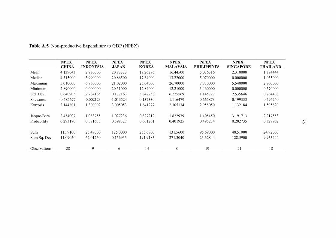
75 75

Table A.5 Non-productive Expenditure to GDP (NPEX)

NPEX_ CHINA

NPEX_ INDONESIA

NPEX_ JAPAN

NPEX_ KOREA

NPEX_ MALAYSIA

NPEX_ PHILIPPINES

NPEX_ SINGAPORE

NPEX_ THAILAND

Mean 4.139643 2.830000 20.83333 18.26286 16.44500 5.036316 2.310000 1.384444 Median 4.315000 3.990000 20.86500 17.64000 13.22000 5.070000 0.000000 1.035000 Maximum 5.010000 6.730000 21.02000 25.04000 26.70000 7.830000 5.540000 2.700000 Minimum 2.890000 0.000000 20.51000 12.84000 12.21000 3.460000 0.000000 0.570000 Std. Dev. 0.640905 2.784165 0.177163 3.842258 6.225569 1.145727 2.535646 0.764408 Skewness -0.585677 -0.002123 -1.013524 0.137330 1.116479 0.665873 0.199333 0.496240 Kurtosis 2.144801 1.300002 3.005053 1.841277 2.305134 2.958050 1.132184 1.595820

Jarque-Bera 2.454007 1.083755 1.027236 0.827212 1.822979 1.405450 3.191713 2.217553 Probability 0.293170 0.581655 0.598327 0.661261 0.401925 0.495234 0.202735 0.329962

Sum 115.9100 25.47000 125.0000 255.6800 131.5600 95.69000 48.51000 24.92000 Sum Sq. Dev. 11.09050 62.01260 0.156933 191.9183 271.3040 23.62844 128.5900 9.933444

Observations 28 9 6 14 8 19 21 18

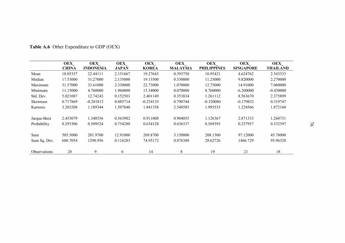
76 76

Table A.6 Other Expenditure to GDP (OEX)

OEX_

CHINA OEX_

INDONESIA OEX_

JAPAN OEX_

KOREA OEX_

MALAYSIA OEX_

PHILIPPINES OEX_

SINGAPORE OEX_

THAILAND Mean 18.05357 22.44111 2.151667 19.27643 0.393750 10.95421 4.624762 2.543333 Median 17.53000 31.27000 2.135000 19.13500 0.330000 11.25000 9.820000 2.270000 Maximum 31.57000 33.61000 2.330000 22.73000 1.070000 12.75000 14.91000 7.060000 Minimum 11.15000 4.760000 1.960000 15.34000 0.070000 8.760000 -6.200000 -0.430000 Std. Dev. 5.021087 12.74243 0.152501 2.401149 0.353834 1.261112 8.563670 2.375899 Skewness 0.717869 -0.281812 0.085714 -0.234135 0.790744 -0.320080 -0.179832 0.319747 Kurtosis 3.203208 1.189344 1.507840 1.841358 2.540585 1.993533 1.224566 1.872160

Jarque-Bera 2.453079 1.348556 0.563982 0.911008 0.904055 1.126367 2.871333 1.260731 Probability 0.293306 0.509524 0.754280 0.634128 0.636337 0.569393 0.237957 0.532397

Sum 505.5000 201.9700 12.91000 269.8700 3.150000 208.1300 97.12000 45.78000 Sum Sq. Dev. 680.7054 1298.956 0.116283 74.95172 0.876388 28.62726 1466.729 95.96320

Observations 28 9 6 14 8 19 21 18

77 77

Table A.7 Budget Surplus to GDP (BS)

BS_

CHINA BS_

INDONESIA BS_

JAPAN BS_

KOREA BS_

MALAYSIA BS_

PHILIPPINES BS_

SINGAPORE BS_

THAILAND Mean -1.161786 -1.473333 -3.961667 0.390000 -0.581250 -2.076842 8.890000 -0.479444 Median -0.960000 -1.300000 -4.135000 0.515000 -0.270000 -1.880000 9.650000 -0.595000 Maximum 0.760000 -0.350000 -0.400000 3.470000 3.910000 0.960000 16.16000 2.140000 Minimum -3.330000 -3.990000 -5.880000 -3.740000 -5.640000 -5.600000 -1.500000 -3.010000 Std. Dev. 0.842180 1.119196 2.017210 1.901291 3.167827 1.981226 4.898831 1.822437 Skewness -0.547800 -1.307190 0.848578 -0.528431 -0.419352 -0.124403 -0.714865 0.148539 Kurtosis 3.762383 3.868559 2.703674 3.223135 2.198055 1.824734 2.775870 1.563419

Jarque-Bera 2.078496 2.846018 0.742037 0.680602 0.448847 1.142498 1.832568 1.614016 Probability 0.353721 0.240988 0.690031 0.711556 0.798977 0.564819 0.400003 0.446191

Sum -32.53000 -13.26000 -23.77000 5.460000 -4.650000 -39.46000 186.6900 -8.630000 Sum Sq. Dev. 19.15021 10.02080 20.34568 46.99380 70.24589 70.65461 479.9710 56.46169

Observations 28 9 6 14 8 19 21 18

78 78

Table A.8 Domestic Investment to GDP (INV)

INV_

CHINA INV_

INDONESIA INV_

JAPAN INV_

KOREA INV_

MALAYSIA INV_

PHILIPPINES INV_

SINGAPORE INV_

THAILAND Mean 32.18000 21.36000 23.51167 31.24786 22.80000 19.43263 28.65143 29.56278 Median 31.37000 21.42000 23.32000 29.96500 22.80000 20.04000 29.50000 23.25000 Maximum 42.54000 23.71000 24.75000 39.33000 24.82000 24.42000 36.25000 42.47000 Minimum 24.95000 19.62000 22.85000 26.87000 20.85000 14.04000 21.93000 19.66000 Std. Dev. 4.869870 1.385496 0.702806 3.998321 1.329049 3.575682 4.057988 9.797593 Skewness 0.616311 0.272961 0.908779 1.190727 0.069965 -0.167667 0.134219 0.263410 Kurtosis 2.612927 1.893440 2.593815 2.934955 2.051534 1.612022 2.267494 1.185547

Jarque-Bera 1.947379 0.570939 0.867126 3.310737 0.306389 1.614155 0.532546 2.677335 Probability 0.377687 0.751661 0.648195 0.191022 0.857963 0.446160 0.766230 0.262195

Sum 901.0400 192.2400 141.0700 437.4700 182.4000 369.2200 601.6800 532.1300 Sum Sq. Dev. 640.3220 15.35680 2.469683 207.8254 12.36460 230.1390 329.3453 1631.878

Observations 28 9 6 14 8 19 21 18

79 79

Table A.9 Export-Import to GDP (EXIM)

EXIM_ CHINA

EXIM_ INDONESIA

EXIM_ JAPAN

EXIM_ KOREA

EXIM_ MALAYSIA

EXIM_ PHILIPPINES

EXIM_ SINGAPORE

EXIM_ THAILAND

Mean 32.63393 55.03333 22.20667 65.06857 136.1463 77.81211 296.7490 93.43444 Median 31.79500 51.46000 20.62500 59.32500 137.9200 82.68000 288.6200 96.10000 Maximum 64.89000 74.89000 28.83000 105.1900 147.4600 114.4800 355.5000 131.9000 Minimum 10.69000 44.42000 18.40000 50.54000 121.0700 46.26000 258.4200 64.99000 Std. Dev. 14.34948 9.227410 4.287585 16.53747 8.544579 21.20803 29.59411 23.56536 Skewness 0.633566 1.034282 0.659383 1.528049 -0.515026 -0.033693 0.786726 0.065490 Kurtosis 3.025517 3.380121 1.807927 4.151924 2.360733 1.703132 2.559368 1.393034

Jarque-Bera 1.873986 1.658795 0.790046 6.222224 0.489889 1.335073 2.336169 1.949623 Probability 0.391804 0.436312 0.673665 0.044551 0.782748 0.512971 0.310962 0.377263

Sum 913.7500 495.3000 133.2400 910.9600 1089.170 1478.430 6231.730 1681.820 Sum Sq. Dev. 5559.508 681.1608 91.91693 3555.341 511.0688 8096.048 17516.23 9440.543

Observations 28 9 6 14 8 19 21 18

80 80

Table A.10 Secondary School Enrollment Ratio (EDUSEC)

EDUSEC_

CHINA EDUSEC_

INDONESIA EDUSEC_

JAPAN EDUSEC_ KOREA

EDUSEC_ MALAYSIA

EDUSEC_ PHILIPPINES

EDUSEC_ SINGAPORE

EDUSEC_ THAILAND

Mean 51.48643 64.97111 101.1133 98.31929 68.63750 76.97895 49.53619 56.15263 Median 50.15500 64.16000 100.9200 97.35500 68.63500 75.41000 46.90000 60.56000 Maximum 71.91000 75.77000 101.9300 106.9000 72.36000 83.73000 75.40000 74.76000 Minimum 38.15000 56.23000 100.6600 92.56000 65.10000 70.44000 37.70000 29.06000 Std. Dev. 11.20015 6.736638 0.458156 4.445237 2.457116 4.270956 10.90807 14.62905 Skewness 0.330007 0.443238 1.002694 0.525051 0.003799 0.198833 1.287877 -0.625210 Kurtosis 1.774594 2.039281 2.697538 2.257557 2.070059 1.762919 3.431868 2.126123

Jarque-Bera 2.260111 0.640808 1.028267 0.964795 0.288283 1.336735 5.968387 1.842376 Probability 0.323015 0.725856 0.598019 0.617302 0.865765 0.512545 0.050580 0.398046

Sum 1441.620 584.7400 606.6800 1376.470 549.1000 1462.600 1040.260 1066.900 Sum Sq. Dev. 3386.968 363.0583 1.049533 256.8817 42.26195 328.3392 2379.720 3852.165

Observations 28 9 6 14 8 19 21 19

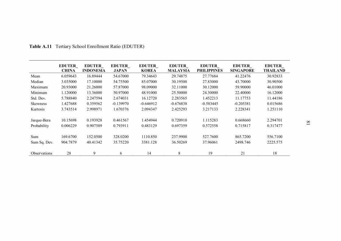
81 81

Table A.11 Tertiary School Enrollment Ratio (EDUTER)

EDUTER_

CHINA EDUTER_

INDONESIA EDUTER_

JAPAN EDUTER_ KOREA

EDUTER_ MALAYSIA

EDUTER_ PHILIPPINES

EDUTER_ SINGAPORE

EDUTER_ THAILAND

Mean 6.059643 16.89444 54.67000 79.34643 29.74875 27.77684 41.22476 30.92833 Median 3.035000 17.10000 54.75500 85.07000 30.19500 27.83000 43.70000 30.90500 Maximum 20.93000 21.26000 57.87000 98.09000 32.11000 30.12000 59.90000 46.01000 Minimum 1.120000 13.36000 50.97000 48.91000 25.50000 24.30000 22.40000 16.12000 Std. Dev. 5.788840 2.247594 2.674031 16.12720 2.283565 1.452213 11.17753 11.44186 Skewness 1.427688 0.359562 -0.139970 -0.646912 -0.676838 -0.583445 -0.205381 0.015686 Kurtosis 3.743514 2.998971 1.670376 2.094347 2.425293 3.217133 2.228341 1.251110

Jarque-Bera 10.15698 0.193928 0.461567 1.454944 0.720910 1.115283 0.668660 2.294701 Probability 0.006229 0.907589 0.793911 0.483129 0.697359 0.572558 0.715817 0.317477

Sum 169.6700 152.0500 328.0200 1110.850 237.9900 527.7600 865.7200 556.7100 Sum Sq. Dev. 904.7879 40.41342 35.75220 3381.128 36.50269 37.96061 2498.746 2225.575

Observations 28 9 6 14 8 19 21 18

82 82

Table A.12 GDP Per Capita Growth (GDPPC)

GDPPC_ CHINA

GDPPC_ INDONESIA

GDPPC_ JAPAN

GDPPC_ KOREA

GDPPC_ MALAYSIA

GDPPC_ PHILIPPINES

GDPPC_ SINGAPORE

GDPPC_ THAILAND

Mean 8.536786 4.971111 -0.511667 4.192857 3.123750 9.314737 4.561905 4.166111 Median 8.630000 5.030000 -0.675000 4.410000 3.625000 9.430000 4.890000 4.700000 Maximum 14.29000 6.350000 2.070000 8.640000 4.840000 13.61000 9.230000 9.160000 Minimum 2.350000 3.450000 -2.280000 -7.620000 -1.580000 5.810000 -4.370000 -11.50000 Std. Dev. 2.858470 1.030600 1.549934 3.985957 1.997648 2.314578 3.784683 4.767093 Skewness -0.286346 -0.244739 0.604720 -1.813577 -1.844477 0.223997 -1.136474 -2.118624 Kurtosis 3.079148 1.713774 2.333047 6.691130 5.137705 2.127316 3.590685 7.671656

Jarque-Bera 0.389947 0.710237 0.476893 15.62207 6.059389 0.761802 4.825802 29.83398 Probability 0.822857 0.701090 0.787851 0.000405 0.048330 0.683246 0.089555 0.000000

Sum 239.0300 44.74000 -3.070000 58.70000 24.99000 176.9800 95.80000 74.99000 Sum Sq. Dev. 220.6130 8.497089 12.01148 206.5421 27.93419 96.43087 286.4765 386.3280

Observations 28 9 6 14 8 19 21 18

ESSAY 2

THAILAND’s FISCAL POLICY IMPACT ANALYSIS

ABSTRACT

This paper examines the dynamic effects of government spending on

Thailand’s economic growth. The analytical methods used in this study are the co-

integration analysis, causality testing, and error correction model between government

spending and economic growth. Contrary to a priori expectation, the findings show

that in the short-run fiscal policy implemented through tax and public spending does

not have significant impact on economic growth. However, in the longer-term, fiscal

policy show discernable impact on growth particularly tax exhibiting negative impact

and government expenditure showing positive impact on growth. However, in the

case of Thailand, public consumption and its components show positive effects on

growth, while public investment does not seem to have positive impact on economic

performance in the longer-term. This serves as a critical illustration for Thai policy-

makers to improve the productivity of Thailand’s public investment spending in the

coming years.

CHAPTER 1

INTRODUCTION

The role of fiscal policy in promoting economic growth has been a controversial

issue among economists and policy-makers. Two contrasting views are put forth by

economic theorists. Classical economists believe in the minimal role for State citing

the preference for market-clearing mechanism and distaste for inefficiency arising

from government intervention, while Keynesian economists take their lesson from the

experiences of Great Depression in 1930s in which they argue that government has an

important role in short-term demand management and longer-term supply management.

Thus, based on Keynesian theory, government actions can determine long-term

economic performance. In the realms of policy-making and public governance, one

can observe the different ideology on the role of State – in the case of the United

States, Republicans generally believe in free market with minimal role for

government, less government spending, and lower taxes. On the other hand,

Democrats argue for more social welfare spending which imply the need for higher

taxes (especially among the rich and wealthy Americans). In many developing

countries including Thailand, the ideology may be less clear cut, but all political

parties seem to now support greater role of government in supporting social welfare

programs implying higher level of government role and spending in the coming years.

Therefore, as we move forward, in-depth analysis of fiscal policy and its impact on

economy will be critical towards ensuring prosperity and sustainable development of

the country. Ultimately, the question will be on how to efficiently and effectively

allocate resources between the public and private sectors. Globally, governments now

actively use fiscal tools to manage the economy and are confident that fiscal policy

can save the world economy from the economic doldrums. However, economists

remain intensely divided over the role of fiscal policy in affecting aggregate demand.

85

Clearly, there remains inconclusive evidence of the relationship between fiscal policy

and economic growth.

This paper aims to address the question whether fiscal policy in Thailand has

been effective in promoting economic development using various econometric

approaches namely VAR model, co-integration analysis, and error correction model.

Not much empirical studies have been done on Thailand and its fiscal policy du to

scarcity of data and limited research interests in this area. Therefore, the main

contribution of this research study is to analyze the relationship between fiscal policy

and economic growth in Thailand which will be crucial for future fiscal policy

formulation.

The study finds that, contrary to a priori expectation, the short-run fiscal

policy implemented through tax and public spending does not have significant impact

on economic growth. However, in the longer-term, fiscal policy show discernable

impact on growth particularly tax exhibiting negative impact and government

expenditure showing positive impact on growth. However, in the case of Thailand,

public consumption and its components show positive effects on growth, while public

investment does not seem to have positive impact on economic performance in the

longer-term. This serves as a critical illustration for Thai policy-makers to improve

the productivity of Thailand’s public investment spending in the coming years.

Background and Research Motivation

The impact of fiscal policy has been controversial issue whether government

expenditure have positive, negative or neutral impact on economic growth. In many

respect, the role of State represent the main argument between the two major schools

of economic thoughts: Classical versus Keynesian economics. They are the two

opposing views are put forth by two great economists – Adam Smith as the father of

Classical economics and John M. Keynes as the originator of Keynesian economics.

Classical economists believe in the minimal role for State citing the preference for

market-clearing mechanism and distaste for inefficiency arising from government

intervention, while Keynesian economists take their lesson from the experiences of

Great Depression in 1930s in which they argue government has an important role in

86

short-term demand management and longer-term supply management. Thus, believers

in Keynesian economics would generally support government role in stimulating

domestic demand through expansionary fiscal policy during times of economic

slowdown, while those who believe in classical economics would argue otherwise that

the economy is best left alone and market mechanism will adjust itself. The severities

of the Asian financial crisis, the U.S. subprime financial crisis in 2008/09, and the on-

going Eurozone debt crisis gives impetus to many government particularly among the

developing countries to deploy their fiscal policy to stipulate domestic economy. In

the case of Thailand, the Asian financial crisis and U.S. sub-prime crisis led to sharp

economic contractions of domestic economy. Asian financial crisis in 1997/98 had

led to unprecedented decline in Thailand’s real GDP at over -10.3 percent in 1998,

while the U.S. financial crisis a decade later caused severe decline on exports and

resulted in economic contraction by -2.2 percent in 2009. As economic growth

plummeted, Thai government implemented expansionary fiscal and monetary policies

to counter the ill-effects of the economic crises. In the context of the Eurozone

sovereign debt crisis and the aftermath of the Thai flood crisis in late-2011 have

prompted the government to plan for greater spending particularly on social welfare

programs and infrastructure development to ensure flood prevention, sustaining

domestic demand momentum, and long-term national competitiveness.

Like many other governments in Asia, Thailand has been turning to activist

fiscal policy ever since the country began the process of economic liberalization in

1950s until today. State directs public spending in the areas of education and

healthcare; improve public administration, transportation infrastructure, and national

security and defense. As the Thai economy grows over the years, government

spending become increasing larger currently at more than 2.0 trillion Baht or 20

percent of national GDP, while tax collection is more than 1.8 trillion Baht or 18

percent of national GDP as of Fiscal Year 2011. Therefore, given that government

would be increasing its role in the economy in the coming years in terms of greater

spending on social welfare programs and infrastructure investment (and the

consequent higher taxes to finance the greater spending?), it would be critical for

policy-makers to better understand the relationship between fiscal policy and

economic growth particularly in the context of Thailand. Therefore, this paper will

87

address the following research questions: 1) what is the short-term and long-run

relationship between fiscal policy and economic growth? Better understanding short-

term and long-term impact would have important implication to fiscal policy

formulation 2) what specific components of fiscal policy that have the most impact on

economic growth? 3) what are the policy recommendations for promoting the positive

role of fiscal policy in Thailand?

In identifying the detailed impact of fiscal policy implementation, the paper

examines the components of taxation (i.e. income-based, consumption-based,

production-based and international-trade-based) as well as expenditures (i.e. public

consumption and public investment). Public expenditures are analyzed in further

details by classifying public consumption into different spending types: 1) General

Administration 2) Defense 3) Justice and Police 4) Education and Research 5) Health

Services 6) Special Welfare Services 7) Transport and Communication Facilities 8)

Other Services. Public investment is classified into: 1) Construction and 2) Equipment

and Machinery.

The justification for focusing on these spending types is that there are some

components of government expenditures that are productive while some are

unproductive. There is a priori belief that government expenditures on public health

and public education should raise labor productivity and hence increase output

growth. Education is one of the important factors that determine the quality of labor

and is indispensable towards achieving high and sustainable economic growth rates

(Hartshone, 1985). Government expenditure on public health could lead to economic

growth because healthy population is the prerequisite for productive workers.

Expenditures on infrastructure such as transportation and communication will bring

about production efficiency and reduction in production costs, which will increase

private sector investment and profitability of firms and thereby fostering economic

growth. National defense spending is a necessity for safeguarding and protecting the

nation from outside aggression hence securing protection of property rights. Welfare

spending is crucial for the well being of the population, but it remains unclear on its

impact on growth. Some say that welfare spending results in disincentive for workers

to be productive and lead to excessive consumption behavior; other argue that welfare

spending promotes social well-being and conducive to productive labor. The role of

88

public investment on growth remains one of the most debated issues in public

economics with some studies find public investment generating positive impact on

growth, while other studies show neutral or even negative impact on growth under the

so-called “crowding-out” effect. This study will aim to provide empirical underpinning

to better understand about the role of government spending on economic growth.

Econometric methodologies namely vector auto-regression model (VAR), co-

integration analysis, and error correction model (ECM) are used as to investigate the

underlying relationship between fiscal policy and economic growth. Afterwards,

policy recommendations can be derived from the empirical findings in this research

study.

CHAPTER 2

LITERATURE REVIEW AND THEORETICAL

MODEL AND METHODOLOGY

There are a number of recent literatures on this topic of fiscal policy and

growth, but much disagreement remains. Indeed, the role of government and fiscal

policy represents the main argument between the two major schools of economic

thoughts: Classical versus Keynesian economics. Two great economists – Adam

Smith as the father of Classical economics and John M. Keynes as the originator of

Keynesian economics – postulated opposing views on the role of government.

Classical economists believe in the minimal role for State citing the preference for

market-clearing mechanism and distaste for inefficiency arising from government

intervention, while Keynesian economists take their lesson from the experiences of

Great Depression in 1930s in which they argue government has an important role in

short-term demand management and longer-term supply management. Thus, believers

in Keynesian economics would generally support government role in stimulating

domestic demand through expansionary fiscal policy during times of economic

slowdown, while those who believe in classical economics would argue otherwise that

the economy is best left alone and market mechanism will adjust itself. Major recent

theoretical and empirical literatures on the role of fiscal policy in the process of

economic development can be traced back to Barro and Sala-i-Martin (1990) and

Easterly and Rebelo (1993). In supporting Keynesian views, both of these studies

identify positive role from specific types of fiscal policy on enhancing economic

growth. In their seminal paper, Barro and Sala-i-Martin (1990) propose that

endogenous economic growth allows for effects of fiscal policy on long-term growth.

If social rate of return on investment exceeds the private return, then tax policies that

encourage investment can raise growth rate and level of utility. Excess of the social

return over the private return can reflect learning-by-doing with spillover effects. Tax

90

incentives for investment are not called for if the private rate of return on investment

equals the social return. Easterly and Rebelo (1993) use cross-section data on

approximately 100 countries for 1970-88 as well as historical data for 28 countries

over 1870-1988 to examine the association between fiscal policy, the level of

development and growth. They find a strong association between the development

level and the fiscal structure: 1) poor countries rely heavily on international trade

taxes, while income taxes are only important in developed economies; 2) fiscal policy

is influenced by the scale of the economy measured by its population (i.e. larger

population countries will tend to have fiscal structure dependent on income taxes); 3)

investment in transport and communication is consistently correlated with growth

while the effects of taxation are difficult to isolate empirically. Since then a large

number of studies have considered the effects of fiscal policy on growth in diverse

countries and regions, applying different methodologies and considering different

types of data. In the empirical literature, most studies apply vector autoregressive

methods aiming at identifying the usual reactions of the aggregate variables to the

exogenous shocks in fiscal policy. For example, Blanchard and Perotti (2002)

examines the dynamic effects of shocks in government spending and taxes on

economic activity in the United States in the post-war period. It does so by using a

mixed structural VAR/event study approach. The results consistently show positive

government spending shocks as having a positive effect on output, and positive tax

shocks as having a negative effect. The multipliers for both spending and tax shocks

are typically small. Turning to the effects of taxes and spending on the components of

GDP, one of the results has a distinctly non-standard outcome with both increases in

taxes and increases in government spending have a strong negative effect on

investment spending. Galí, López-Salido, and Vallés (2007) find that a government

spending leads to a significant increase in consumption, while investment either falls

or does not respond significantly. Thus, their evidence seems to be consistent with the

predictions of IS-LM type models (predicting positive relationship between

government spending and growth), and hard to reconcile with those of the neoclassical

paradigm (predicting no or even negative relationship between government spending

and growth). They postulate that the interaction of consumers with sticky prices and

deficit financing can account for the existing evidence on the effects of government

91

spending. Consumers insulate part of aggregate consumption from the negative

wealth effects generated by the higher levels of (current and future) taxes needed to

finance the fiscal expansion, while making it more sensitive to current labor income

(net of current taxes). Sticky prices make it possible for real wages to increase, even

if the marginal product of labor goes down, since the price markup may decline

sufficiently to more than offset the latter effect. The increase in the real wage raises

current labor income and hence stimulates the consumption of households. That

intuition explains why both nominal rigidities in wages and prices are needed in order

to obtain the desired pro-cyclical response of consumption. Burriel et al. (2009) paper

analyses the effects of fiscal policy in the euro area as a whole by employing a new

database containing quarterly fiscal variables. They use the methodology developed

by Blanchard and Perotti (2002) to identify fiscal shocks within a SVAR framework.

Apart from the results for the euro area itself, they compare them with those obtained

for the U.S. for the same sample period. In general, their results find that GDP and

inflation increase in response to government spending shocks, although output

multipliers are, in general, very similar in both areas and small, typically below unity.

On the other hand, government expenditure shocks show a higher degree of

persistence in the U.S., which seems to be explained by the persistence of military

spending. In turn, net-tax increases weight on economic activity, with the negative

response being shorter-lived in the euro area. In any case, these effects do not appear

sizeable. In line with previous studies, they find that tax multipliers are lower than

spending ones in the short-term. As for the reaction of the main GDP components,

private consumption displays similar pattern responses to GDP in both the euro area

and the US. Private investment responses are not so homogeneous though: it declines

in response to higher government spending or net taxes in the US, whereas in the

EMU only tax increases seem to entail a negative reaction of private investment.

Mountford and Uhlig (2009) analyze the effects of fiscal policy using vector auto-

regressions. Specifically, they use sign restrictions to identify a government revenue

shock as well as a government spending shock, while controlling for a generic

business cycle shock and a monetary policy shock. They explicitly allow for the

possibility of announcement effects, i.e., that a current fiscal policy shock changes

fiscal policy variables in the future, but not at present. They construct the impulse

92

responses to three linear combinations of these fiscal shocks, corresponding to the

three scenarios of deficit-spending, deficit-financed tax cuts and a balanced budget

spending expansion. They apply the method to U.S. quarterly data from 1955-2000.

They find that deficit-financed tax cuts work best among these three scenarios to

improve GDP, with a maximal present value multiplier of five dollars of total

additional GDP per each dollar of the total cut in government revenue five years after

the shock.

However, other research papers show mixed evidence and most of these

papers focus on countries of the Organization for Economic Co-operation and

Development (OECD), G7, and other industrial economies. However, based on a

meta-analysis of a sample of 93 published studies, Nijkamp and Poot (2004) provide

evidence that on balance, the positive effect of conventional fiscal policy on growth is

rather weak. In their study, a sample of 93 published studies, yielding 123 meta-

observations, is used to examine the robustness of the evidence regarding the effect of

fiscal policy on growth. Five fiscal policy areas are considered: general government

consumption, tax rates, education expenditure, defense, and public infrastructure.

Several meta-analytical techniques are applied, including descriptive statistics,

contingency table analysis and rough set analysis. On balance, as mentioned earlier,

the evidence for a positive effect of conventional fiscal policy on growth is rather

weak, but the commonly identified importance of education and infrastructure is

confirmed. The results are sensitive to several research design parameters, such as the

type of data, model specification and econometric technique.

However, according to Spilimbergo, Symansky, and Schindler (2009), the

overall evidence from the literature indicates that the multiplier for government

spending is larger than that for tax cuts. They put forth the following rule of thumb for

government consumption: a multiplier of 1–1.5 in large countries; 0.5–1 in medium-

size countries; and 0.5 or less in small open economies. The same rule of thumb

postulates multipliers of only about half the above values for tax cuts and transfer

payments and slightly larger multipliers for government investment. Baldacci, Gupta,

and Mulas-Granados (2009) studies the effects of fiscal policy response in 118

episodes of systemic banking crisis in advanced and emerging market countries

during 1980–2008. Their study finds that timely countercyclical fiscal measures

93

contribute to shortening the length of crisis episodes by stimulating aggregate

demand. Fiscal expansions that rely mostly on measures to support government

consumption are more effective in shortening the crisis duration than those based on

public investment or income tax cuts. But these results do not hold for countries with

limited fiscal space where fiscal expansions are prevented by funding constraints. The

composition of countercyclical fiscal responses matters as well for output recovery

after the crisis, with public investment yielding the strongest impact on growth. These

results suggest a potential trade-off between short-run aggregate demand support and

medium-term productivity growth objectives in fiscal stimulus packages adopted in

distress times. Romer and Bernstein (2009) estimated the multipliers of government

spending by the United States and tax cuts to be 1.57 and 0.99, respectively.

Interestingly, a number of studies contradict the intuitively plausible notion that

government spending has a bigger impact on output than tax cuts. Romer and Romer

(2009) find that one dollar of tax cuts historically raised US gross domestic product

(GDP) by about three dollars. A multiplier of 3 is far higher than most of the

estimated multipliers for government spending. For example, the empirical results of

Ramey (2009) uses standard Vector Auto Regression (VAR) identification methods to

find uncertain impact on government spending raising consumption and real wages

with the implied government spending multipliers range from 0.6 to 1.2.

However, the findings of Romer and Romer (2009) are not alone in suggesting

a stronger impact of tax cuts. Using the U.S. data, Mountford and Uhlig (2009), find

that deficit-financed tax cuts have a bigger effect than deficit-financed spending or tax

financed spending. Moreover, they find that the long term costs of fiscal expansion

through government spending are probably greater than the short term gains. In

similar findings, Alesina and Ardagna (2009) examine the evidence on episodes of

large stances in fiscal policy, both in cases of fiscal stimuli and in that of fiscal

adjustments in OECD countries from 1970 to 2007. They find that fiscal stimuli based

upon tax cuts are more likely to increase growth than those based upon spending

increases. As for fiscal adjustments those based upon spending cuts and no tax

increases are more likely to reduce deficits and debt over GDP ratios than those based

upon tax increases. In addition, adjustments on the spending side rather than on the

tax side are less likely to create recessions. They confirm these results with simple

94

regression analysis. Blanchard and Perotti (2002) examine the dynamic effects of

shocks in government spending and taxes on U.S. activity in the postwar period.

Using a mixed structural VAR/event study approach with identification achieved by

using institutional information about the tax and transfer systems, they identify the

automatic response of taxes and spending to activity, and, by implication, to infer

fiscal shocks. The results consistently show positive government spending shocks as

having a positive effect on output, and positive tax shocks as having a negative effect.

However, one result has a distinctly nonstandard flavor: both increases in taxes and

increases in government spending have a strong negative effect on investment

spending. Similarly, Mountford and Uhlig (2009) find the cumulative multipliers for

revenue (tax) shocks for the U.S. to be typically greater than the spending shocks; and

both increases in taxes and increases in government spending have a negative effect

on consumption and investment spending. This suggests a possible explanation for

why some studies find tax cuts to be more expansionary than government spending.

Tax cuts may further boost output by stimulating investment while the positive effect

of government spending may be largely offset by lower private investment. Perotti

(1999) also examines the 1980s period in which several countries with large

government debt or deficit implemented substantial, and in some cases drastic, deficit

cuts. Contrary to widespread expectations, in many cases private consumption

boomed rather than contract. This paper shows that in times of “fiscal stress” shocks

to government revenues and, especially, expenditure have very different effects on

private consumption than in “normal” times. In this context, for the US, Cogan et al.

(2010) find that the government spending multipliers from permanent increases in

federal government purchases are much less in new Keynesian models than in old

Keynesian models, with the multipliers being less than one as consumption and

investment are crowded out, turning negative as the government purchases decline in

the later years of their simulation. Hemming, Kell and Mahfouz (2002), who

summarize theoretical and empirical literature on the effectiveness of fiscal policy in

stimulating economic growth, note that given data deficiencies and institutional

weaknesses, there is no clear conclusion on the size and sign of fiscal multipliers in

developing countries. Unlike a plethora of studies on industrialized countries debating

whether tax cuts are more effective than government spending, there is only limited

95

evidence about the issue in the Asia and Pacific region. To some extent, this simply

mirrors the fact that industrialized countries have a longer tradition of using fiscal

policy for countercyclical purposes than developing countries such as Thailand, which

have accorded a higher priority to growth rather than output stability. For example,

automatic stabilizers such as unemployment benefits are an integral part of fiscal

policy in the G3 but an underdeveloped novelty in much of the developing countries.

On the other hand, there are some studies that find their support in the

Classical viewpoint or find Keynesian views inconclusive. Ram (1986a) undertakes

panel data study for 63 countries found limited support to government sector

expenditure rising with growth in national income. On the other hand, Abizadeh and

Gray (1985) for 55 countries found support for a rise in the share of government

sector in national income in the case of rich countries but not for poor countries.

Chen (2003) using data from 6 developed countries (Canada, France, Germany, Italy,

UK, and USA) and 3 developing countries (Korea, Singapore and Taiwan) during

1972 to 1992 conducted regression analyses with the proportion of public expenditure

to GDP and economic growth rate. They found that economic growth rates declined

along with increases of the proportion of public expenditure to GDP. Al-Faris (2002)

examined the nature of the relationship between government expenditure and

economic growth in the Gulf Cooperation Council countries. In his study, Al-Faris

(2002) found that national income is a predictive factor of the expanding role of

government and not the other way around. Thus, his empirical investigations do not

support the Keynesian theory. Other studies such as Hondroyiannis and Papapetrou

(1996) for Demirbas (1999) for Turkey also find no evidence of any long-run

relationship between government sector expenditure and national income. Ghali

(1997) analyzed the relationship between government expenditure and economic

growth in Saudi Arabia by examining the intertemporal interactions among the

growth rate in per capita real GNP and the share of government spending in national

income. Ghali found no consistent evidence that government spending can increase

Saudi Arabia’s per capita output growth.

There are studies that find mixed results for fiscal policy impact on growth.

Hansson and Henrekson (1994) find that government consumption spending is

growth-retarding but spending on education impacts positively on growth. Kneller et al

96

(1998) found that productive spending has a positive, while non-productive spending

has a negative impact on growth of OECD countries. Ram (1986b), using a sample of

115 countries, found government expenditure to have significant positive externality

effects on growth particularly in the developing countries sample, but total

government spending had a negative effect on growth in the developing countries.

Lin (1994), in contrast, found that nonproductive spending had no effect on growth in

the advanced countries but a positive impact in LDCs. As noted above, most of the

empirical studies are cross-section, and specific country case studies are rare. Time

series analysis for specific countries can avoid some of the econometric and sampling

problems. Specifically, cross-section analysis assumes that the coefficients are the

same for all countries in the sample whereas time series analysis can address country-

specific features. A time series country study like this study for Thailand could

potentially be more informative, although the findings may not be generalized to other

countries.

Therefore, it remains unclear whether proactive use of fiscal policy would

result in economic growth. Given that the Thai government would be increasing its

role in the economy in the coming years in terms of greater spending on social

welfare programs and infrastructure investment, it would be critical for the country’s

policy-makers to better understand the relationship between fiscal policy and

economic growth particularly in the context of Thailand. Therefore, this paper will

empirically examine the short-term and long-term association between fiscal policy

and economic growth, and identify specific components of fiscal policy that have the

most impact on output growth. In identifying the specific details of fiscal policy, the

paper will examine in details in the components of taxation (i.e. income-based,

consumption-based, production-based and international-trade-based) as well as

expenditures (i.e. public consumption and public investment). Public expenditures

are studied in further details by classifying public consumption into spending types:

1) General Administration 2) Defense 3) Justice and Police 4) Education and

Research 5) Health Services 6) Special Welfare Services 7) Transport and

Communication Facilities 8) Other Services. Public investment is classified into: 1)

Construction and 2) Equipment. VAR model, Co-integration analysis, and Error

Correction Model (ECM) will be used as empirical methodologies for investigating

the relationship between fiscal policy and economic growth.

97

Conceptual Framework and Methodology

To examine the relationship between fiscal policy and growth, this study will employ vector auto-regression (VAR) analysis, co-integration analysis, and Error Correction Model (ECM).

1) Vector Auto-Regression Analysis This paper applies the structural vector autoregressive approach proposed by

Blanchard and Perotti (2002). Both government expenditure and taxation affect GDP: since the two are presumably not independent, to estimate the effects of one it is also necessary to include the other. Hence, the paper focuses on two-variable breakdowns of fiscal policy, consisting of expenditure and revenue variables. Expenditure variable is defined as total purchases of goods and services, i.e. public consumption plus public investment. Revenue variable is defined as total net revenues.

The paper will also examine in details the specific components of tax and expenditure and its growth implications. Therefore, revenue variable will be tested in the model such as 1) total tax revenue 2) income-based tax 3) consumption-based, 4) production based tax and 5) international-trade-based. Expenditures will be classified into 1) public consumption and 2) public investment. Sub-components of public expenditures will also be considered: Public consumption can be broken down into spending types: 1) General Administration 2) Defense 3) Justice and Police 4) Education and Research 5) Health Services 6) Special Welfare Services 7) Transport and Communication Facilities 8) Other Services. Public investment can be broken into: 1) Construction and 2) Equipment.

VAR Specification

The basic VAR specification is:

...……………………………………………………………..(1)

tttt XGTY ,, is a three-dimensional vector in the logarithms of quarterly taxes,

spending, and GDP, all in real, per capita terms. The paper uses quarterly data

because this is essential for identification of the fiscal shocks.

ttt UYqLAY 1),(

98

tttt xgtU ,, is the corresponding vector of reduced form residuals, which in general

will have non-zero cross correlations.

),( qLA is a four-quarter distributed lag polynomial that allows for the coefficients at

each lag to depend on the particular quarter q that indexes the dependent variable. The

reason for allowing for quarter-dependence of the coefficients is the presence of

seasonal patterns in the response of taxes to economic activity. Some taxes—such as

indirect taxes, or income taxes when withheld at the source—are paid with minimal

delays relative to the time of transaction. Other taxes—such as corporate income

taxes—are often paid with substantial delays relative to the time of the transaction; in

addition, if the bulk of the payment is made in one or two specific quarters of the

year, the delay varies depending on the quarter. For example, in Thailand, corporate

income taxes are paid in May (for the second half of the previous year’s earning) and

August (for the first half of the current year’s estimated earning). Thus, a corporate

income tax is paid in the second quarter (specifically in May) of each year, for activity

over the previous year.

Denoting the three variables as taxes ( tx ), government spending ( s ), and real GDP

( y ) gives:

yt

st

txt

yt

st

txt

yt

st

st

txt

yt

txt

ubaa

ububaububa

333213

222123

121113

…………………………………………............... (2-4)

Equation (2) says that unexpected movements in taxes in the current quarter ( tx

t ) are

related to unexpected movements in economic activity ( yt ), structural shocks to taxes

( txtu ), and structural shocks to government spending ( s

tu ). The same applies to

Equation (3), for unexpected movements in government spending. Equation (4)

relates unexpected movements in economic activity ( yt ) to unexpected movements in

both taxes and government spending, as well as its own structural shocks ( ytu ).

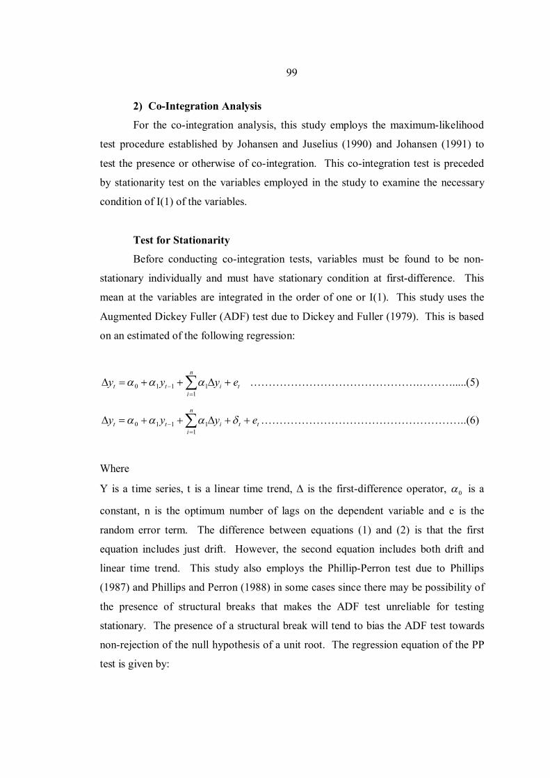
99

2) Co-Integration Analysis

For the co-integration analysis, this study employs the maximum-likelihood

test procedure established by Johansen and Juselius (1990) and Johansen (1991) to

test the presence or otherwise of co-integration. This co-integration test is preceded

by stationarity test on the variables employed in the study to examine the necessary

condition of I(1) of the variables.

Test for Stationarity

Before conducting co-integration tests, variables must be found to be non-

stationary individually and must have stationary condition at first-difference. This

mean at the variables are integrated in the order of one or I(1). This study uses the

Augmented Dickey Fuller (ADF) test due to Dickey and Fuller (1979). This is based

on an estimated of the following regression:

ti

n

itt eyyy

11110 ……………………………………….……….....(5)

tti

n

itt eyyy

11110 ………………………………………………..(6)

Where

Y is a time series, t is a linear time trend, Δ is the first-difference operator, 0 is a

constant, n is the optimum number of lags on the dependent variable and e is the

random error term. The difference between equations (1) and (2) is that the first

equation includes just drift. However, the second equation includes both drift and

linear time trend. This study also employs the Phillip-Perron test due to Phillips

(1987) and Phillips and Perron (1988) in some cases since there may be possibility of

the presence of structural breaks that makes the ADF test unreliable for testing

stationary. The presence of a structural break will tend to bias the ADF test towards

non-rejection of the null hypothesis of a unit root. The regression equation of the PP

test is given by:

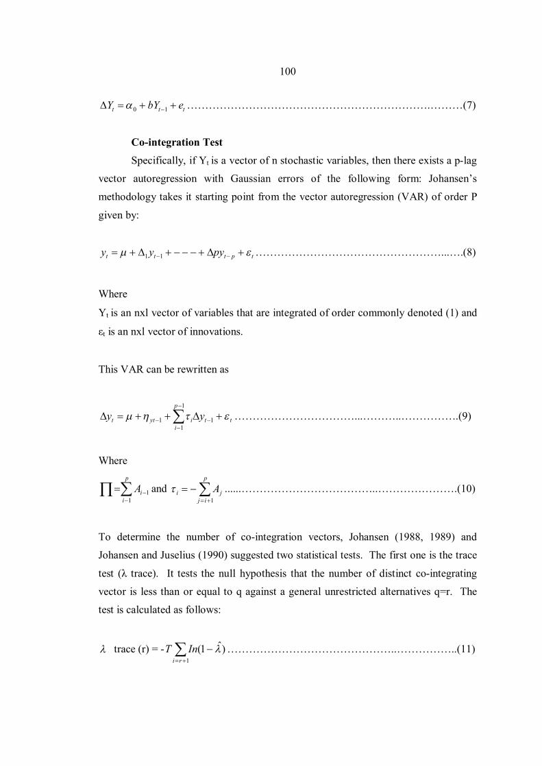
100

ttt ebYY 10 ………………………………………………………….………(7)

Co-integration Test

Specifically, if Yt is a vector of n stochastic variables, then there exists a p-lag

vector autoregression with Gaussian errors of the following form: Johansen’s

methodology takes it starting point from the vector autoregression (VAR) of order P

given by:

tpttt pyyy 11 ……………………………………………...….(8)

Where

Yt is an nxl vector of variables that are integrated of order commonly denoted (1) and

εt is an nxl vector of innovations.

This VAR can be rewritten as

tt

p

iiytt yy

1

1

11 ……………………………...………..…………….(9)

Where

p

iiA

11 and

p

ijji A

1 ......………………………………..………………….(10)

To determine the number of co-integration vectors, Johansen (1988, 1989) and

Johansen and Juselius (1990) suggested two statistical tests. The first one is the trace

test (λ trace). It tests the null hypothesis that the number of distinct co-integrating

vector is less than or equal to q against a general unrestricted alternatives q=r. The

test is calculated as follows:

trace (r) = - )ˆ1(1

ri

InT ………………………………………..……………..(11)

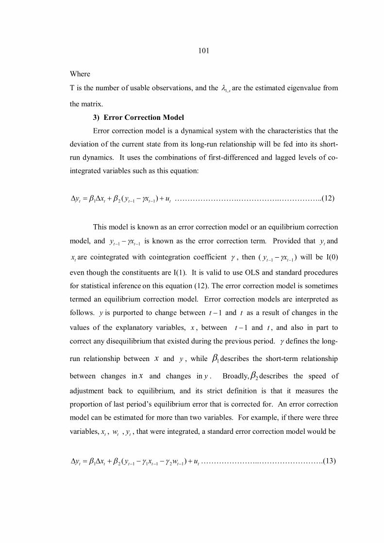
101

Where

T is the number of usable observations, and the s,1 are the estimated eigenvalue from

the matrix.

3) Error Correction Model

Error correction model is a dynamical system with the characteristics that the

deviation of the current state from its long-run relationship will be fed into its short-

run dynamics. It uses the combinations of first-differenced and lagged levels of co-

integrated variables such as this equation:

ttttt uxyxy )( 1121 …………………….…………….……………..(12)

This model is known as an error correction model or an equilibrium correction

model, and 11 tt xy is known as the error correction term. Provided that ty and

tx are cointegrated with cointegration coefficient , then ( 11 tt xy ) will be I(0)

even though the constituents are I(1). It is valid to use OLS and standard procedures

for statistical inference on this equation (12). The error correction model is sometimes

termed an equilibrium correction model. Error correction models are interpreted as

follows. y is purported to change between 1t and t as a result of changes in the

values of the explanatory variables, x , between 1t and t , and also in part to

correct any disequilibrium that existed during the previous period. defines the long-

run relationship between x and y , while 1 describes the short-term relationship

between changes in x and changes in y . Broadly, 2 describes the speed of

adjustment back to equilibrium, and its strict definition is that it measures the

proportion of last period’s equilibrium error that is corrected for. An error correction

model can be estimated for more than two variables. For example, if there were three

variables, tx , tw , ty , that were integrated, a standard error correction model would be

tttttt uwxyxy )( 1211121 …………………..…………………….(13)

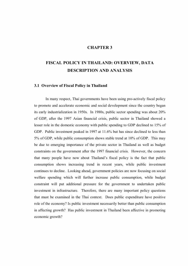
CHAPTER 3

FISCAL POLICY IN THAILAND: OVERVIEW, DATA

DESCRIPTION AND ANALYSIS

3.1 Overview of Fiscal Policy in Thailand

In many respect, Thai governments have been using pro-actively fiscal policy

to promote and accelerate economic and social development since the country began

its early industrialization in 1950s. In 1980s, public sector spending was about 20%

of GDP, after the 1997 Asian financial crisis, public sector in Thailand showed a

lesser role in the domestic economy with public spending to GDP declined to 15% of

GDP. Public investment peaked in 1997 at 11.6% but has since declined to less than

5% of GDP, while public consumption shows stable trend at 10% of GDP. This may

be due to emerging importance of the private sector in Thailand as well as budget

constraints on the government after the 1997 financial crisis. However, the concern

that many people have now about Thailand’s fiscal policy is the fact that public

consumption shows increasing trend in recent years, while public investment

continues to decline. Looking ahead, government policies are now focusing on social

welfare spending which will further increase public consumption, while budget

constraint will put additional pressure for the government to undertaken public

investment in infrastructure. Therefore, there are many important policy questions

that must be examined in the Thai context. Does public expenditure have positive

role of the economy? Is public investment necessarily better than public consumption

in affecting growth? Has public investment in Thailand been affective in promoting

economic growth?

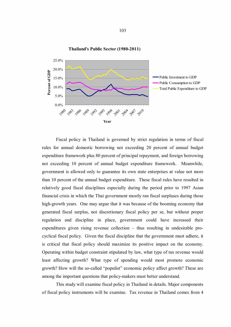
103

Thailand's Public Sector (1980-2011)

0.0%

5.0%

10.0%

15.0%

20.0%

25.0%

1980

1983

1986

1989

1992

1995

1998

2001

2004

2007

2010

Year

Perc

ent o

f GD

P

Public Investment to GDPPublic Consumption to GDPTotal Public Expenditure to GDP

Fiscal policy in Thailand is governed by strict regulation in terms of fiscal

rules for annual domestic borrowing not exceeding 20 percent of annual budget

expenditure framework plus 80 percent of principal repayment, and foreign borrowing

not exceeding 10 percent of annual budget expenditure framework. Meanwhile,

government is allowed only to guarantee its own state enterprises at value not more

than 10 percent of the annual budget expenditure. These fiscal rules have resulted in

relatively good fiscal disciplines especially during the period prior to 1997 Asian

financial crisis in which the Thai government mostly ran fiscal surpluses during those

high-growth years. One may argue that it was because of the booming economy that

generated fiscal surplus, not discretionary fiscal policy per se, but without proper

regulation and discipline in place, government could have increased their

expenditures given rising revenue collection – thus resulting in undesirable pro-

cyclical fiscal policy. Given the fiscal discipline that the government must adhere, it

is critical that fiscal policy should maximize its positive impact on the economy.

Operating within budget constraint stipulated by law, what type of tax revenue would

least affecting growth? What type of spending would most promote economic

growth? How will the so-called “populist” economic policy affect growth? These are

among the important questions that policy-makers must better understand.

This study will examine fiscal policy in Thailand in details. Major components

of fiscal policy instruments will be examine. Tax revenue in Thailand comes from 4

104

main sources: income tax, consumption tax, production tax, and international trade

tax. Most of tax revenue in Thailand is income-based tax (i.e. corporate income tax,

personal income tax). Consumption-based tax (i.e. VAT) has secondary role as major

source of government revenue. Production-based tax (i.e. excise tax) also represents

the third largest share of government revenue. However, production based tax in

Thailand may not represent the overall industrial output of Thailand as excise tax are

levied on sin products such as alcohol and tobacco. This means that higher excise tax

collection may not necessarily good for economic well-being if the revenue increase

comes at the expense of higher alcohol and tobacco production and consumption.

Finally, international trade tax shows declining trend as Thailand has been lowering

its tariff rates through WTOs and FTAs. It would be interesting to know which type

of tax would be least negative impact on economic growth.

Tax revenue structure

0%

20%

40%

60%

80%

100%

1996

1998

2000

2002

2004

2006

2008

2010

Year

Prop

ortio

n

International TradeTaxProduction Tax

Consumption Tax

Income Tax

In terms of public spending, it can be categorized into two major types: public

consumption and public investment. Public consumption can be classified into various

types. Education and research absorbs the largest share of public consumption

followed by general administration. Defense spending shows declining share over the

years. Looking ahead, health services and special welfare services are expected to

increase their share as Thailand enters into aging society. It would be interesting to

see how each types of public consumption affect growth.

105

Public consumption

0%

20%

40%

60%

80%

100%

1996

1998

2000

2002

2004

2006

2008

2010

Year

Prop

ortio

n

Other services

Transport and CommunicationFacilities

Special welfare services

Health services

Education and Research

Justice and Police

Defense

General Administration

Public investment can be classified into: Construction investment and

Equipment & Machinery investment. Construction investment commands the larger

share of public investment. It would be interesting to analyze which type of public

investment has larger growth impact.

Public Investment

0%20%40%60%80%

100%

1996

1998

2000

2002

2004

2006

2008

2010

Year

Prop

ortio

n

EquipmentConstruction

3.2 Data Description and Analysis

In this study, fiscal data for Thailand are quarterly data covering the period

from 1996Q1 to 2010Q4. The data in the study are as follows:

Public Consumption

106

Table 3.1 Data Sources

Data Sources

1. Gross Domestic Product NESDB

2. Population CEIC

3. Net government revenue FPO

3.1 Total tax revenue FPO

3.1.1 Income tax FPO

3.1.2 Consumption tax FPO

3.1.3 Production tax FPO

3.1.4 International trade tax FPO

4. Total public expenditure NESDB

4.1 Public consumption NESDB

4.1.1 Defense NESDB

4.1.2 Justice and police NESDB

4.1.3 Education and research NESDB

4.1.4 Health services NESDB

4.1.5 Special welfare services NESDB

4.1.6 Transport and communication facilities NESDB

4.1.7 Other services NESDB

4.2 Public investment NESDB

4.2.1 Construction NESDB

4.2.2 Equipment NESDB

Note: 1. NESDB denotes National Economic and Social Development Board,

Thailand 2. CEIC denotes CEIC Database Company Limited 3. FPO denotes Fiscal Policy Office, Ministry of Finance, Thailand

The data are adjusted into real terms with GDP deflator (to be constant 1988 prices) and express in per capita basis. Furthermore, the variables are adjusted into log form, seasonal adjusted, first difference for stationary. The data set are as shown in the Appendix.

107

Thailand’s fiscal data during the period from 1996:Q1 to 2010:Q4 can be

summarized as follows:

1. Nominal GDP + Real GDP 2. GDP Deflator –

3. GDP per capita (Real) 4. Net Government Revenue

(Nominal) + Net Government

Revenue (Real)

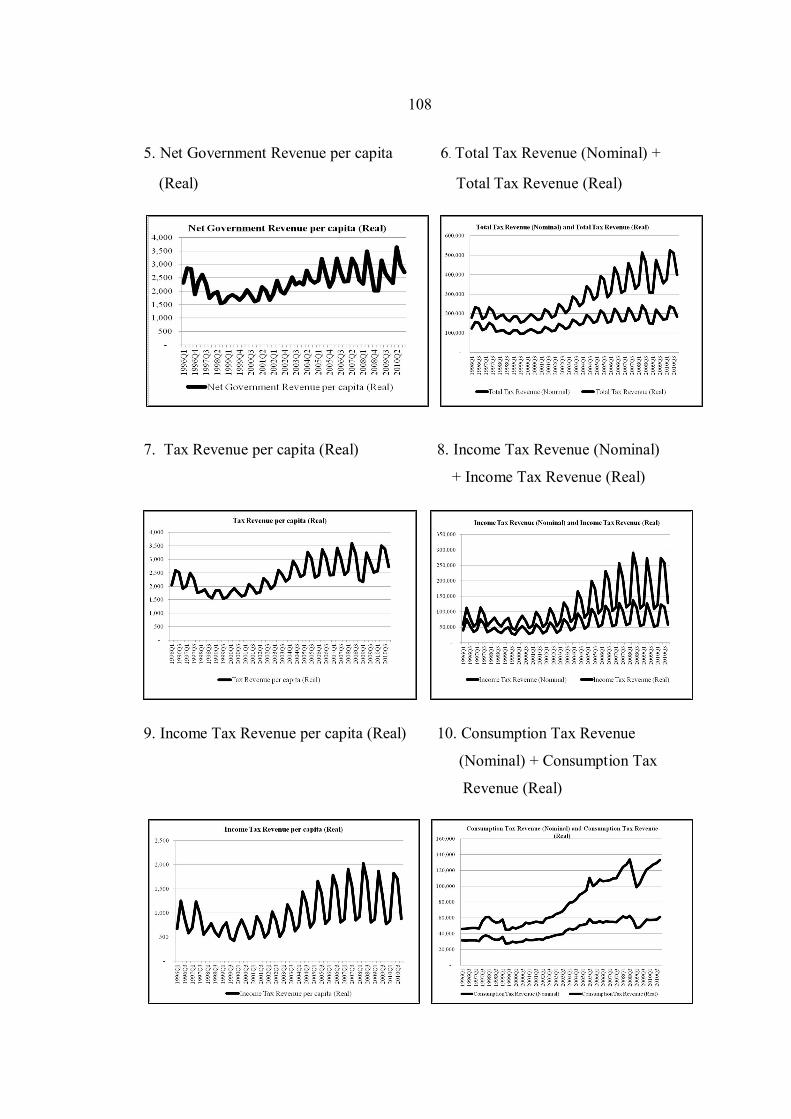
108

5. Net Government Revenue per capita 6. Total Tax Revenue (Nominal) +

(Real) Total Tax Revenue (Real)

7. Tax Revenue per capita (Real) 8. Income Tax Revenue (Nominal)

+ Income Tax Revenue (Real)

9. Income Tax Revenue per capita (Real) 10. Consumption Tax Revenue

(Nominal) + Consumption Tax

Revenue (Real)

109

11. Consumption Tax Revenue per capita 12. Production Tax Revenue

(Real) (Nominal) + Production Tax

Revenue (Real)

13. Production Tax Revenue per capita 14. International Trade Tax

(Real) Revenue (Nominal) +

International Trade Tax

Revenue (Real)

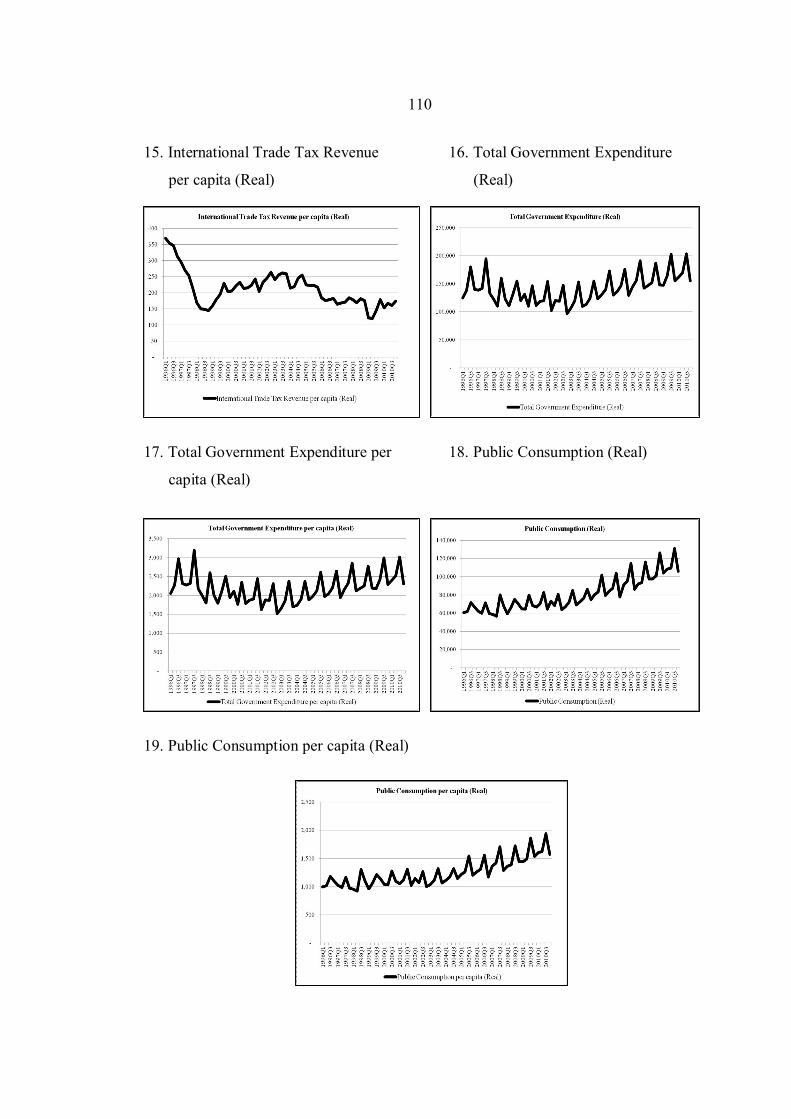
110

15. International Trade Tax Revenue 16. Total Government Expenditure

per capita (Real) (Real) 17. Total Government Expenditure per 18. Public Consumption (Real)

capita (Real)

19. Public Consumption per capita (Real)

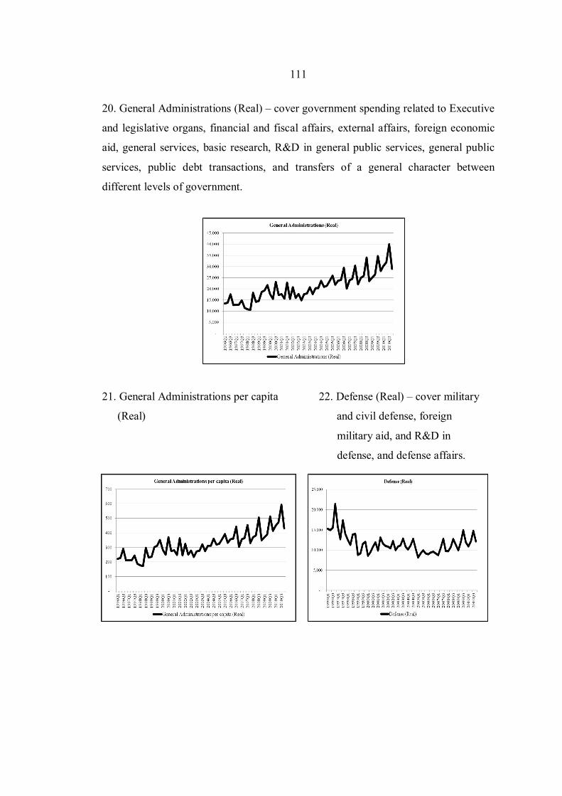
111

20. General Administrations (Real) – cover government spending related to Executive

and legislative organs, financial and fiscal affairs, external affairs, foreign economic

aid, general services, basic research, R&D in general public services, general public

services, public debt transactions, and transfers of a general character between

different levels of government.

21. General Administrations per capita 22. Defense (Real) – cover military

(Real) and civil defense, foreign

military aid, and R&D in

defense, and defense affairs.

112

23. Defense per capita (Real)

24. Justice and Police (Real) cover government spending related to Police services

fire-protection services, law courts, prisons, R&D in public order and safety, and

public order and safety affairs.

25. Justice and Police per capita (Real)

113

26. Education and Research (Real) cover government spending related to pre-primary

and primary education, secondary education, post-secondary non-tertiary education,

tertiary education, education not definable by level, subsidiary services to education,

R&D in education and education affairs.

27. Education and Research per capita (Real) 28. Health Services (Real) - Medical

products, appliances and

equipment, outpatient services,

hospital services, public health

services, R&D in health, and

health affairs

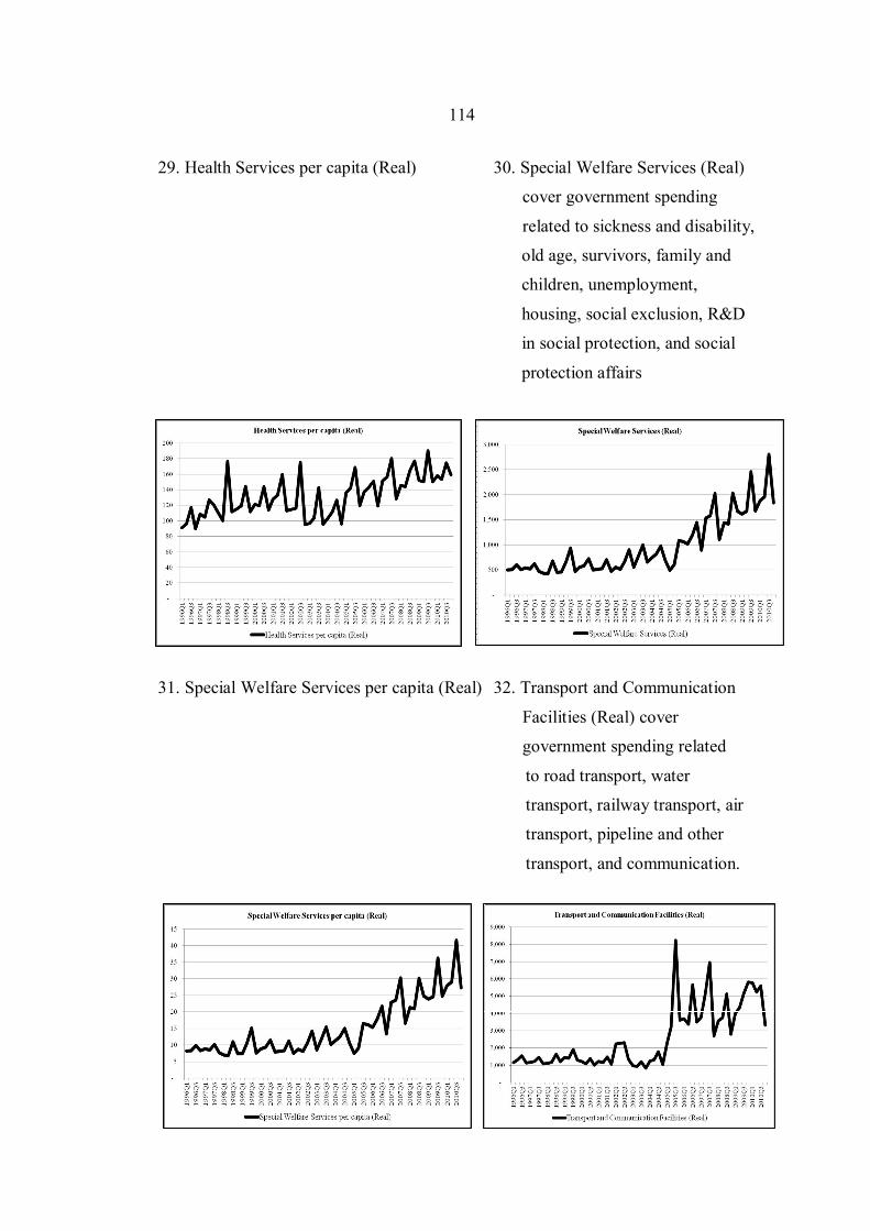
114

29. Health Services per capita (Real) 30. Special Welfare Services (Real)

cover government spending

related to sickness and disability,

old age, survivors, family and

children, unemployment,

housing, social exclusion, R&D

in social protection, and social

protection affairs

31. Special Welfare Services per capita (Real) 32. Transport and Communication

Facilities (Real) cover

government spending related

to road transport, water

transport, railway transport, air

transport, pipeline and other

transport, and communication.

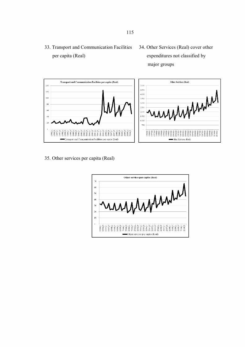
115

33. Transport and Communication Facilities 34. Other Services (Real) cover other

per capita (Real) expenditures not classified by

major groups

35. Other services per capita (Real)

116

36. Public Investment (Real) is the acquisition less disposal of nonfinancial assets

(excluding valuables, if possible). It covers the public acquisitions of capital assets

classified into 1) construction investment and 2) machinery and equipment

investment.

37. Public Investment per capita (Real)

117

38. Public construction investment (Real) covers construction activities undertaken by

central government, local authorities, and state-owned enterprises. It covers investment

in constructions of dwelling; buildings other than dwellings include whole buildings

or parts of buildings not designated as dwellings. Fixtures, facilities and equipment

that are integral parts of the structures are included. Other structures include structures

other than buildings, including the cost of the streets, sewer, etc.

39. Public construction Investment per capita (Real)

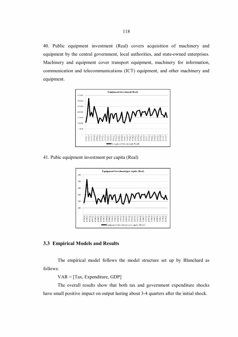
118

40. Public equipment investment (Real) covers acquisition of machinery and

equipment by the central government, local authorities, and state-owned enterprises.

Machinery and equipment cover transport equipment, machinery for information,

communication and telecommunications (ICT) equipment, and other machinery and

equipment. 41. Pubic equipment investment per capita (Real)

3.3 Empirical Models and Results

The empirical model follows the model structure set up by Blanchard as

follows:

VAR = [Tax, Expenditure, GDP]

The overall results show that both tax and government expenditure shocks

have small positive impact on output lasting about 3-4 quarters after the initial shock.

119

Impulse response of GDP to tax

shocks

Quarter after shocks

Impulse response of GDP to spending

shocks

Quarter after shocks

However, the finding for government spending shocks having positive impact on output growth in Thailand is consistent with the a priori hypothesis that fiscal spending should have a positive relationship to growth. However, the positive relationship between tax shocks that output seems to be inconsistent with economic theory as well as Blanchard’s finding that indicates negative relationship between tax shocks and output growth in the U.S. economy. Moreover, positive relationship between production based tax and output should be taken with some caution as it may not represent the overall industrial output of Thailand as excise tax are levied on sin products such as alcohol and tobacco. This means that higher excise tax collection may not necessarily good for economic well-being if the revenue increase comes at the expense of higher alcohol and tobacco production and consumption.

However, it may be necessary to consider models in which government expenditure as exogenous variable. This is aimed to show the impact of tax shocks on GDP while controlling the effect from government expenditure. This is done to exclude the impact from government expenditure. Given that the result indicates that tax shock has positive impact on GDP growth, we may then hypothesize that it is because positive tax shock increases government expenditure and, therefore, increases GDP – not because tax shock directly by itself positively impacts GDP.

Thus, the models are as follows: VAR = [Tax, GDP] with government expenditure as exogenous variable. The result shows that tax shocks has a small positive impact on the output

growth.

120

Impulse Response of GDP to Tax Shocks (Government Expenditure as Exogenous)

Quarter after shocks

3.3.1 Components of Tax and Government Expenditure As mentioned earlier, tax and government expenditure can be classified into

their components to assess the impact on output growth. The VAR models to examine the economic impact of these fiscal components are as follows:

1) VAR = [income tax revenue, government expenditure, GDP] 2) VAR = [consumption tax revenue, government expenditure, GDP] 3) VAR = [production tax revenue, government expenditure, GDP] 4) VAR = [international trade tax revenue, government expenditure,

GDP] 5) VAR = [tax revenue, public consumption expenditure, GDP] 6) VAR = [tax revenue, public investment expenditure, GDP] 7) VAR = [tax revenue, general administration expenditure, GDP] 8) VAR = [tax revenue, defense expenditure, GDP] 9) VAR = [tax revenue, justice and police expenditure, GDP] 10) VAR = [tax revenue, education and research expenditure, GDP] 11) VAR = [tax revenue, health services expenditure, GDP] 12) VAR = [tax revenue, special welfare services expenditure, GDP] 13) VAR = [tax revenue, transport and communication facilities

expenditure, GDP] 14) VAR = [tax revenue, other consumption expenditure, GDP]

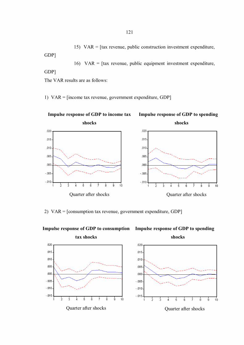
121

15) VAR = [tax revenue, public construction investment expenditure,

GDP]

16) VAR = [tax revenue, public equipment investment expenditure,

GDP]

The VAR results are as follows:

1) VAR = [income tax revenue, government expenditure, GDP]

Impulse response of GDP to income tax

shocks

Quarter after shocks

Impulse response of GDP to spending

shocks

Quarter after shocks

2) VAR = [consumption tax revenue, government expenditure, GDP]

Impulse response of GDP to consumption

tax shocks

Quarter after shocks

Impulse response of GDP to spending

shocks

Quarter after shocks

122

3) VAR = [production tax revenue, government expenditure, GDP]

Impulse response of GDP to production

tax shocks

Quarter after shocks

Impulse response of GDP to spending

shocks

Quarter after shocks

4) VAR = [international trade tax revenue, government expenditure, GDP]

Impulse response of GDP to international

tax shocks

Quarter after shocks

Impulse response of GDP to spending

shocks

Quarter after shocks

123

5) VAR = [tax revenue, public consumption expenditure, GDP]

Impulse response of GDP to tax revenue

shocks

Quarter after shocks

Impulse response of GDP to public

consumption shocks

Quarter after shocks

6) VAR = [tax revenue, public investment expenditure, GDP]

Impulse response of GDP to tax revenue

shocks

Quarter after shocks

Impulse response of GDP to public

investment shocks

Quarter after shocks

124

7) VAR = [tax revenue, public investment expenditure, GDP]

Impulse response of GDP to tax revenue

shocks

Quarter after shocks

Impulse response of GDP to general

administration shocks

Quarter after shocks

8) VAR = [tax revenue, defense expenditure, GDP]

Impulse response of GDP to tax revenue

shocks

Quarter after shocks

Impulse response of GDP to defense

expenditure shocks

Quarter after shocks

125

9) VAR = [tax revenue, justice and police expenditure, GDP]

Impulse response of GDP to tax

revenue shocks

Quarter after shocks

Impulse response of GDP to justice

and police expenditure shocks

Quarter after shocks

10) VAR = [tax revenue, education and research expenditure, GDP]

Impulse response of GDP to tax

revenue shocks

Quarter after shocks

Impulse response of GDP to education

and research expenditure shocks

Quarter after shocks

126

11) VAR = [tax revenue, health services expenditure, GDP]

Impulse response of GDP to tax

revenue shocks

Quarter after shocks

Impulse response of GDP to health

service expenditure shocks

Quarter after shocks

12) VAR = [tax revenue, special welfare services expenditure, GDP]

Impulse response of GDP to tax

revenue shocks

Quarter after shocks

Impulse response of GDP to special

welfare services expenditure shocks

Quarter after shocks

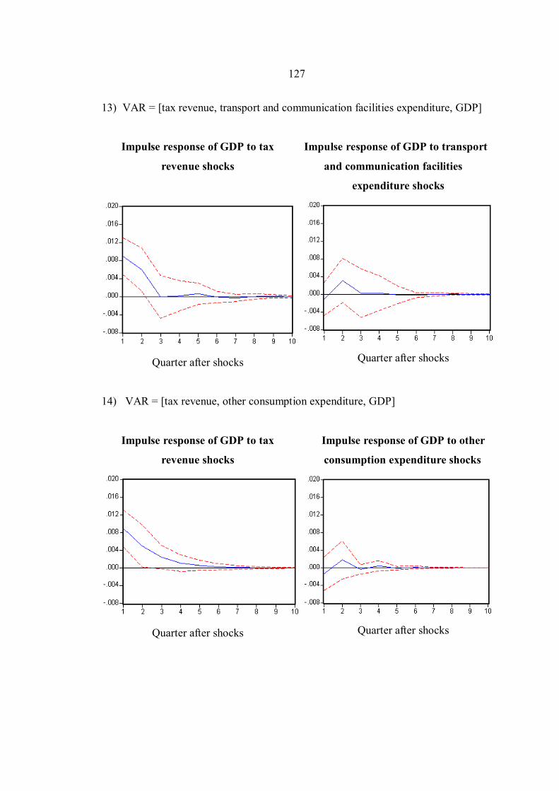
127

13) VAR = [tax revenue, transport and communication facilities expenditure, GDP]

Impulse response of GDP to tax

revenue shocks

Quarter after shocks

Impulse response of GDP to transport

and communication facilities

expenditure shocks

Quarter after shocks

14) VAR = [tax revenue, other consumption expenditure, GDP]

Impulse response of GDP to tax

revenue shocks

Quarter after shocks

Impulse response of GDP to other

consumption expenditure shocks

Quarter after shocks

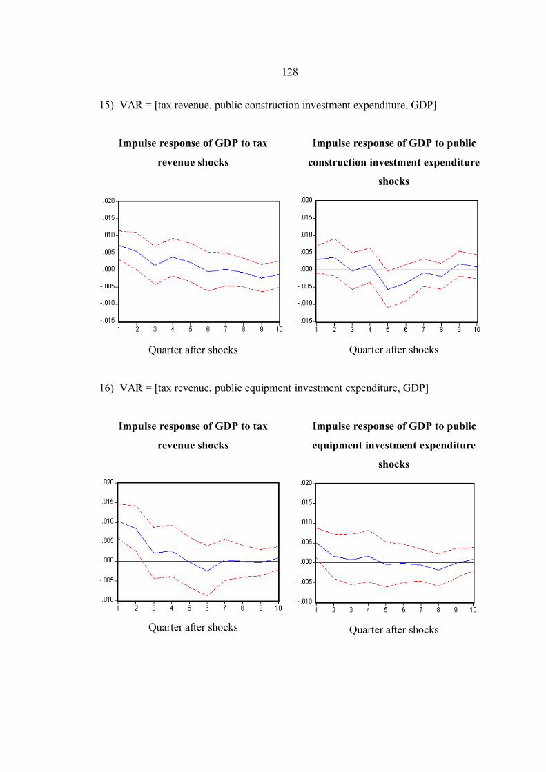
128

15) VAR = [tax revenue, public construction investment expenditure, GDP]

Impulse response of GDP to tax

revenue shocks

Quarter after shocks

Impulse response of GDP to public

construction investment expenditure

shocks

Quarter after shocks

16) VAR = [tax revenue, public equipment investment expenditure, GDP]

Impulse response of GDP to tax

revenue shocks

Quarter after shocks

Impulse response of GDP to public

equipment investment expenditure

shocks

Quarter after shocks

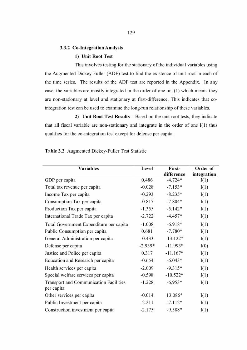
129

3.3.2 Co-Integration Analysis

1) Unit Root Test

This involves testing for the stationary of the individual variables using

the Augmented Dickey Fuller (ADF) test to find the existence of unit root in each of

the time series. The results of the ADF test are reported in the Appendix. In any

case, the variables are mostly integrated in the order of one or I(1) which means they

are non-stationary at level and stationary at first-difference. This indicates that co-

integration test can be used to examine the long-run relationship of these variables.

2) Unit Root Test Results – Based on the unit root tests, they indicate

that all fiscal variable are non-stationary and integrate in the order of one I(1) thus

qualifies for the co-integration test except for defense per capita.

Table 3.2 Augmented Dickey-Fuller Test Statistic

Variables Level First-difference

Order of integration

GDP per capita 0.486 -4.724* I(1) Total tax revenue per capita -0.028 -7.153* I(1) Income Tax per capita -0.293 -8.235* I(1) Consumption Tax per capita -0.817 -7.804* I(1) Production Tax per capita -1.355 -5.142* I(1) International Trade Tax per capita -2.722 -4.457* I(1)

Total Government Expenditure per capita -1.008 -6.918* I(1) Public Consumption per capita 0.681 -7.780* I(1) General Administration per capita -0.433 -13.122* I(1) Defense per capita -2.939* -11.993* I(0) Justice and Police per capita 0.317 -11.167* I(1) Education and Research per capita -0.654 -6.043* I(1) Health services per capita -2.009 -9.315* I(1) Special welfare services per capita -0.598 -10.522* I(1) Transport and Communication Facilities per capita

-1.228 -6.953* I(1)

Other services per capita -0.014 13.086* I(1) Public Investment per capita -2.211 -7.112* I(1) Construction investment per capita -2.175 -9.588* I(1)

130

Table 3.2 (Continued)

Variables Level First-difference

Order of integration

Equipment investment per capita -2.753 -6.346* I(1) Private Consumption per capita 0.222 -4.845* I(1) Private Investment per capita -2.417 -3.655* I(1) Export of G&S per capita -0.958 -5.565* I(1)

Note: 1. Augmented Dickey-Fuller Test – Lag length: 3 (Automatic based on SIC.

MAXLAG = 9) otherwise stated.

2. * value denotes significance at 5% level.

3) Co-Integration Analysis – Based on the co-integration results below,

they indicate that growth and tax revenue have positive long-run relationship.

However, growth and public expenditure also have larger in magnitude of positive

long-run relationship particularly for public investment. Within public consumption

classification, spending on education and health have larger long-run growth effect

than spending on welfare. Between the two types of public investment, equipment &

machinery investment shows slightly higher positive long-run effect than construction

investment.

Co-integration results indicate that income tax revenue have positive

long-term relationship with economic growth, while international trade tax revenue

have negative long-term relationship with economic growth. Health service spending

also has positive long-run relationship with economic growth as good public health is

critical towards human productivity. Finally, public investment has long-term positive

relationship with output growth, although the relationship is quite small and comes

from construction-related investment. Co-integration relationships between fiscal

variables (relevant tax revenue and public expenditures) and output growth are as

follows:

131

Table 3.3 Co-Integration Test Results

Fiscal variables

Lag Trace Statistics

Critical Value (0.05)

P-value Normalized Co-

integrating Coefficient

Tax Revenue per capita 3 25.93088 29.79707 0.1308 -2.548869

(0.36646)

Income Tax per capita 3 29.25550 29.79707 0.0576 -2.690878

(0.21837)

Consumption Tax per

capita

3 30.57640 29.79707 0.0406 -0.859183

(0.33712)

Production Tax per capita 2 15.88401 29.79707 0.7204 -4.262029

(1.25056)

International Trade Tax per

capita

2 33.71147 29.79707 0.0168 1.514922

(0.37052)

Total Government

Expenditure per capita

3 25.93088 29.79707 0.1308 -0.729350

(0.18426)

Public Consumption per

capita

3 22.11496 29.79707 0.2922 -1.471940

(0.33595)

General Administration per

capita

2 15.06088 29.79707 0.7761 -3.498003

(0.74456)

Defense per capita 3 20.41659 29.79707 0.3950 -3.308609

(1.77965)

Justice and Police per

capita

3 19.10904 29.79707 0.4851 -1.920588

(0.23171)

Education and Research per

capita

3 19.25936 29.79707 0.4744 -1.039998

(0.23322)

Health services per capita 3 28.97337 29.79707 0.0620 -3.026213

(0.39677)

Special welfare services per

capita

3 19.72138 29.79707 0.4419 -7.731786

(0.92061)

132

Table 3.3 (Continued)

Fiscal variables

Lag Trace Statistics

Critical Value (0.05)

P-value Normalized Co-

integrating Coefficient

Tax Revenue per capita 3 25.93088 29.79707 0.1308 -2.548869

(0.36646)

Transport and

Communication Facilities

per capita

3 25.95922 29.79707 0.1299 -7.167569

(1.66309)

Other services per capita 3 17.09462 29.79707 0.6331 -4.026669

(0.86404)

Public Investment per

capita

3 27.89043 29.79707 0.0817 -0.449128

(1.05700)

Construction investment

per capita

3 34.37881 29.79707 0.0138 -0.896158

(1.15390)

Equipment investment per

capita

3 19.82757 29.79707 0.4346 0.289861

(0.80865)

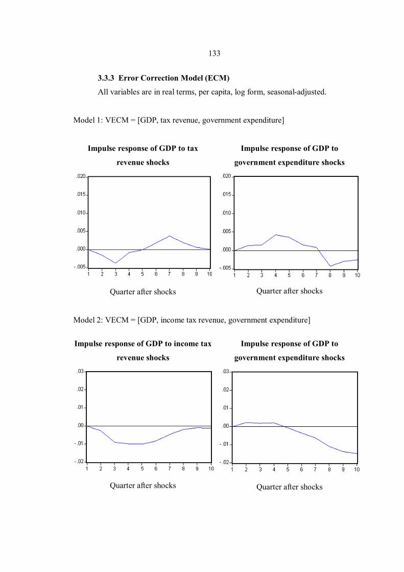
133

3.3.3 Error Correction Model (ECM)

All variables are in real terms, per capita, log form, seasonal-adjusted.

Model 1: VECM = [GDP, tax revenue, government expenditure]

Impulse response of GDP to tax

revenue shocks

Quarter after shocks

Impulse response of GDP to

government expenditure shocks

Quarter after shocks

Model 2: VECM = [GDP, income tax revenue, government expenditure]

Impulse response of GDP to income tax

revenue shocks

Quarter after shocks

Impulse response of GDP to

government expenditure shocks

Quarter after shocks

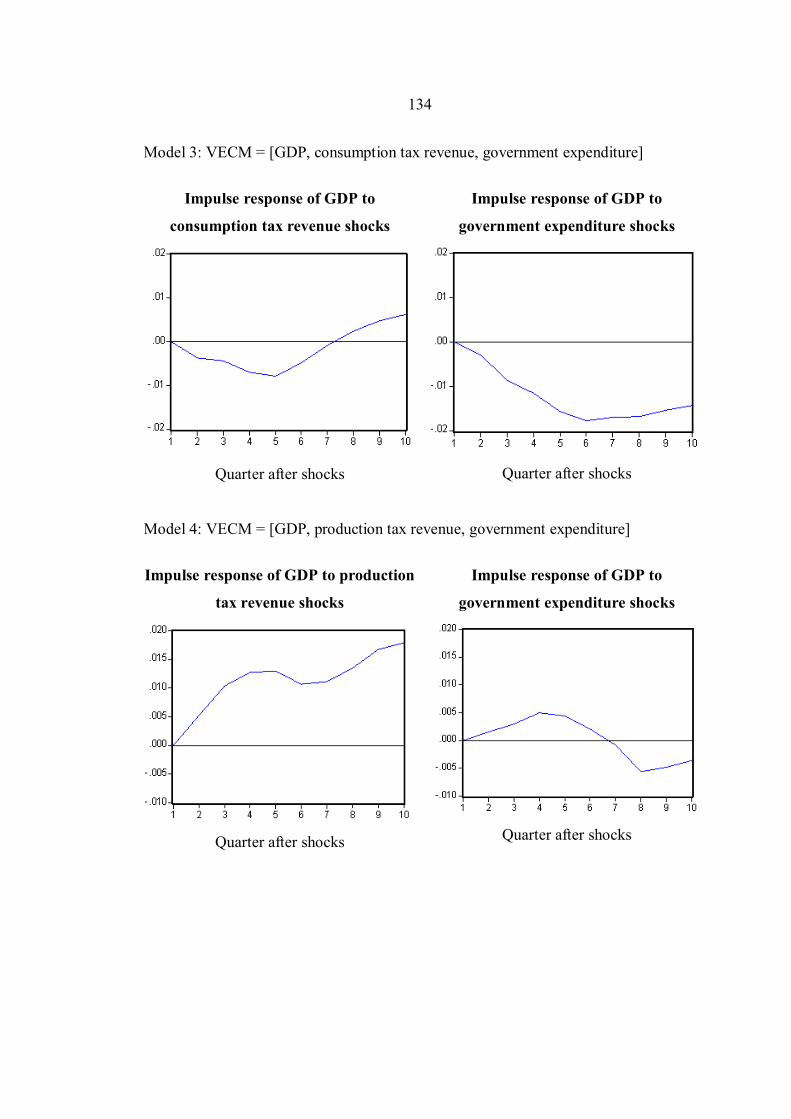
134

Model 3: VECM = [GDP, consumption tax revenue, government expenditure]

Impulse response of GDP to

consumption tax revenue shocks

Quarter after shocks

Impulse response of GDP to

government expenditure shocks

Quarter after shocks

Model 4: VECM = [GDP, production tax revenue, government expenditure]

Impulse response of GDP to production

tax revenue shocks

Quarter after shocks

Impulse response of GDP to

government expenditure shocks

Quarter after shocks

135

Model 5: VECM = [GDP, international trade tax revenue, government expenditure]

Impulse response of GDP to

international trade tax revenue shocks

Quarter after shocks

Impulse response of GDP to

government expenditure shocks

Quarter after shocks

Model 6: VECM = [GDP, total tax revenue, public consumption expenditure]

Impulse response of GDP to total tax

revenue shocks

Quarter after shocks

Impulse response of GDP to public

consumption shocks

Quarter after shocks

136

Model 7: VECM = [GDP, total tax revenue, general administration expenditure]

Impulse response of GDP to total tax

revenue shocks

Quarter after shocks

Impulse response of GDP to general

administration expenditure shocks

Quarter after shocks

Model 8: VECM = [GDP, total tax revenue, defense expenditure]

Impulse response of GDP to total tax

revenue shocks

Quarter after shocks

Impulse response of GDP to defense

expenditure shocks

Quarter after shocks

137

Model 9: VECM = [GDP, total tax revenue, justice and police expenditure]

Impulse response of GDP to total tax

revenue shocks

Quarter after shocks

Impulse response of GDP to justice and

police expenditure shocks

Quarter after shocks

Model 10: VECM = [GDP, total tax revenue, education and research expenditure]

Impulse response of GDP to total tax

revenue shocks

Quarter after shocks

Impulse response of GDP to education

and research expenditure shocks

Quarter after shocks

138

Model 11: VECM = [GDP, total tax revenue, health services expenditure]

Impulse response of GDP to total tax

revenue shocks

Quarter after shocks

Impulse response of GDP to health

services expenditure shocks

Quarter after shocks

Model 12: VECM = [GDP, total tax revenue, special welfare services expenditure]

Impulse response of GDP to total tax

revenue shocks

Quarter after shocks

Impulse response of GDP to special

welfare expenditure shocks

Quarter after shocks

139

Model 13: VECM = [GDP, total tax revenue, transport and communication facilities expenditure]

Impulse response of GDP to total tax

revenue shocks

Quarter after shocks

Impulse response of GDP to transport

and communication facilities expenditure

shocks

Quarter after shocks

Model 14: VECM = [GDP, total tax revenue, other services expenditure]

Impulse response of GDP to total tax

revenue shocks

Quarter after shocks

Impulse response of GDP to other services

expenditure shocks

Quarter after shocks

140

Model 15: VECM = [GDP, total tax revenue, public investment expenditure] Impulse response of GDP to total tax

revenue shocks

Quarter after shocks

Impulse response of GDP to public

investment expenditure shocks

Quarter after shocks

Model 16: VECM = [GDP, total tax revenue, construction investment expenditure]

Impulse response of GDP to total tax

revenue shocks

Quarter after shocks

Impulse response of GDP to construction

investment expenditure shocks

Quarter after shocks

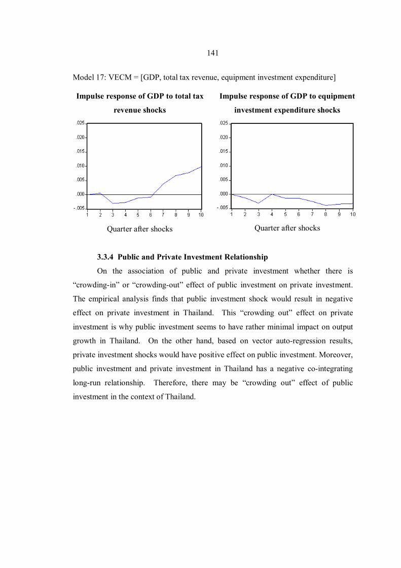
141

Model 17: VECM = [GDP, total tax revenue, equipment investment expenditure] Impulse response of GDP to total tax

revenue shocks

Quarter after shocks

Impulse response of GDP to equipment

investment expenditure shocks

Quarter after shocks

3.3.4 Public and Private Investment Relationship

On the association of public and private investment whether there is

“crowding-in” or “crowding-out” effect of public investment on private investment.

The empirical analysis finds that public investment shock would result in negative

effect on private investment in Thailand. This “crowding out” effect on private

investment is why public investment seems to have rather minimal impact on output

growth in Thailand. On the other hand, based on vector auto-regression results,

private investment shocks would have positive effect on public investment. Moreover,

public investment and private investment in Thailand has a negative co-integrating

long-run relationship. Therefore, there may be “crowding out” effect of public

investment in the context of Thailand.

142

VAR = [Public Investment, Private Investment]

Impulse response of private investment

to public investment shocks

Quarter after shocks

Impulse response of public investment

to private investment shocks

Quarter after shocks

Co-integration = [Public Investment, Private Investment]

Variables

Lag Trace Statistics

Critical Value (0.05)

P-value Normalized Co-integrating

Coefficient Private investment 2 28.43853 29.79707 0.0003 0.452675

(0.14887)

Public investment 2 28.43853 29.79707 0.0003 2.209091

(0.68180)

143

VECM = [Public Investment, Private Investment]

Impulse response of private investment

to public investment shocks

Quarter after shocks

Impulse response of public investment

to private investment shocks

Quarter after shocks

3.3.5 Policy Recommendations This paper examines the dynamic effects of government spending on

Thailand’s economic growth. The analytical methods used in this study are the co-integration analysis, causality testing, and error correction model between government spending and economic growth. Contrary to a priori expectation, the findings show that in the short-run fiscal policy implemented through tax and public spending does not have significant impact on economic growth. However, in the longer-term, fiscal policy show discernable impact on growth particularly tax exhibiting negative impact and government expenditure showing positive impact on growth. However, in the case of Thailand, public consumption and its components show positive effects on growth, while public investment does not seem to have positive impact on economic performance in the longer-term. The policy recommendations based on the findings of this study are as follows:

1) Fiscal policy does have impact on growth in both positive and negative ways. Tax policy often generate negative impact on economic growth in which the government must consider the costs and benefits of implementing specific tax policies in order to minimize economic distortions and to ensure that the negative effect from rising the fiscal resources would be offset by the positive effect after the fiscal resources are deployed through spending policies.

144

2) Public expenditures can have positive impact on growth by its

provisions of public goods, infrastructure development, national security, law and

order. However, some public spending generates more positive economic effects than

others. Public expenditure policy should reorient spending towards more productive

types in order to maximize the positive impact on economic growth and development.

3) Public investment in Thailand has not generated discernable

positive growth impact on the economy. It may be possible that the public investment

data from 1996-2010 used in the study does not really come from productive

infrastructure investment, but public investment in recent years has been undertaken

in unproductive buildings and constructions. Furthermore, in the classification of

public expenditure, education and public health are categorized as government

consumption expenditure. However, good education and public health are critical

inputs for human capital formation. Possibly, these spending should also be

considered as public investment which may add to increasing productivity of public

investment and its overall impact on economic growth. In any case, it is critical for

policy-makers to reexamine government investment policies to increase the

productivity of public investment in Thailand.

Therefore, Thai policy-makers need to reorient government consumption

expenditure toward higher growth impact and reexamine public investment decisions

to ensure that they are conductive to growth and promote productivity in the medium-

term. The findings from this paper serve as a critical illustration for Thai policy-

makers to improve the productivity of Thailand’s public spending in the coming

years.

BIBLIOGRAPHY

Abizadeh, S. and Gray, J. 1985. Wagner's Laws: A Pooled Time-Series, Cross-

Section Comparison. National Tax Journal. 38: 209–218.

Al-Faris, A. F. 2002. Public Expenditure and Economic Growth in the Gulf

Cooperation Council Countries. Applied Economics. 34: 1187-1193.

Alesina, A. and Ardagna, S. 2009. Large Changes in Fiscal Policy: Taxes Versus

Spending. NBER Working Paper 15438. Cambridge: National Bureau of

Economic Research.

Amjad, R. and Din, M. 2009. Economic and Social Impact of Global Financial

Crisis: Implications for Macroeconomic and Development Policies in

South Asia. Islamabad: Pakistan Institute of Development Economics.

Baldacci, E.; Gupta, S. and Mulas-Granados, C. 2009. How Effective is Fiscal

Policy Response in Systemic Banking Crises? IMF Working Paper

WP/09/160. Washington, DC.: International Monetary Fund.

Barro, Robert J. and Sala-i-Martin, Xavier. 1990. Government Spending in a Simple

Model of Endogenous Growth. Journal of Political Economy. 98, 5,

Part II: S103-S125.

Blanchard, O. and Perotti, R. 2002. An Empirical Characterization of the Dynamic

Effects of Changes in Government Spending and Taxes on Output.

Quarterly Journal of Economics. 117 (4): 1329–1368.

Burnside, C.; Eichenbaum, M. and Fisher, J. 2003. Fiscal Shocks and Their

Consequences. Journal of Economic Theory. 115 (1): 89–117.

Burriel, P.; De Castro, F.; Garrote, D.; Gordo, E.; Paredes, J. and Pérez, J. J. 2009.

Fiscal Policy Shocks in the Euro Area and the US: An Empirical

Assessment. Working Paper Series No. 1133. Frankfurt: European

Central Bank.

Caldara, D. and Kamps, C. 2008. What are the Effects of Fiscal Shocks? A VAR-

Based Comparative Analysis. Working Paper Series No. 877. Frankfurt:

European Central Bank.

146

Chen, B. L. 2003. Tax Evasion in a Model of Endogenous Growth. Review of

Economic Dynamics. 6: 381–403.

Cogan, J. F.; Cwik, T.; Taylor, J. B. and Wieland, V. 2010. New Keynesian Versus

Old Keynesian Government Spending Multipliers. Journal of Economic

Dynamics and Control. 34 (3): 281–295.

Demirbaş, S. 1999. Cointegration Analysis–Causality Testing and Wagner's

Law: The Case of Turkey, 1950-1990. Discussion Papers, 99/2

University of Leicester.

Dickey, D. A. and Fuller, W. A. 1979. Distribution of the Estimators for

Autoregressive Time Series with a Unit Root. Journal of the American

Statistical Association. 74: 427–431.

Easterly, W. and Rebelo, S. 1993. Fiscal Policy and Economic Growth. Journal of

Monetary Economics. 32 (3):417–458.

Eskesen, L. B. 2009a. Countering the Cycle—The Effectiveness of Fiscal Policy

in Korea. IMF Working Paper No. 09/249. Washington, DC.:

International Monetary Fund.

Eskesen, L. B. 2009b. The Role for Counter-Cyclical Fiscal Policy in Singapore.

IMF Working Paper No. 09/8. Washington, DC.: International Monetary

Fund.

Galí, J.; López-Salido, J. D. and Vallés, J. 2007. Understanding the Effects of

Government Spending on Consumption. Journal of the European

Economic Association. 5 (1):227–270.

Ghali, K. H. 1997. Government Spending and Economic Growth in Saudi Arabia.

Journal of Economic Development. 22 (2): 165-172.

Hansson, P and Henrekson, M. 1994. A New Framework for Testing the Effect of

Government Spending on Growth and Productivity. Public Choice. 8:

381-401.

Hartshone, K. B. 1985. Education and Development in the South African

Context. Johannesburg: Development in Southern African.

Hemming, R.; Kell, M. and Mahfouz, S. 2002. The Effectiveness of Fiscal Policy

in Stimulating Economic Activity—A Review of the Literature. IMF

Working Paper No. WP/02/208. Washington, DC. : International

Monetary Fund.

147

Hondroyiannis, G. and Papapetrou, E. 1996. International Banking Activity in

Greece: The Recent Experience. Journal of Economics and Business.

48: 207–215.

Johansen, S. 1988. Statistical Analysis of Cointegration Vectors. Journal of

Economic Dynamics and Control. 12: 231–254.

Johansen, S. 1989. Likelihood Based Inference on Cointegration: Theory and

Applications. Lecture Notes (Institute of Mathematical Statistics,

University of Copenhagen, Copenhagen).

Johansen, Soren and Juselius, Katarina. 1990. Maximum Likelihood Estimation and

Inference on Cointegration--With Applications to the Demand for Money.

Oxford Bulletin of Economics and Statistics (Department of Economics,

University of Oxford). 52 (2): 169-210.

Johansen, S. 1991. Estimation and Hypothesis Testing of Cointegrated Vectors in.

Gaussian Vector Autoregressive Models. Econometrica. 59 (6): 1551-

1580.

Kneller, R.; Bleaney, M. and Gemmell, N. 1998. Fiscal Policy and Growth:

Evidence from OECD Countries. Journal of Public Economics. 74:

171-190.

Lin, S. 1994. Government Spending and Economic Growth: Applied Economics.

26 (1): 83-94.

Linnemann, L. and Schabert, A. 2006. Productive Government Expenditure in

Monetary Business Cycle Models. Scottish Journal of Political

Economy. 53 (1): 28–46.

Mountford, A. and Uhlig, H. 2009. What are the Effects of Fiscal Policy Shocks?

Journal of Applied Econometrics. 24 (6): 960–992.

Nijkamp, P. and Poot, J. 2004. Meta-Analysis of the Effect of Fiscal Policies on

Long-Run Growth. European Journal of Political Economy. 20 (1):

91–124.

Pappa, E. 2009. The Effects of Fiscal Shocks on Employment and the Real Wage.

International Economic Review. 50: 217–244.

Perotti, R. 1999. Fiscal Policy in Good Times and Bad. Quarterly Journal of

Economics. 114 (4): 1399–1436.

148

Phillips, P. C. B and Perron, P. 1988. Testing for a Unit Root in Time Series

Regression. Biometrika. 75: 335–346.

Ram, Rati. 1986a. Government Size and Economic Growth: A New Framework and

Some Evidence from Cross-Section and Time-Series Data. American

Economic Review. 76: 191-203.

Ram, Rati. 1986b. Wagner’s Hypothesis in Time Series and Cross Section

Perspectives: Evidence from ‘Real’ Data for 115 Countries. Review of

Economics and Statistics. 69: 194-204.

Ramey, V. 2009. Identifying Government Spending Shocks: It's All in the

Timing. NBER Working Paper 15464. Cambridge: National Bureau of

Economic Research.

Romer, C. and Bernstein, J. 2009. The Job Impact of the American Recovery and

Reinvestment Plan. Washington D.C.: Office of the Vice-President

Romer, Christina and Romer, David. 2009. Do Tax Cuts Starve the Beast? The

Effect of Tax Changes on Government Spending. Brookings Papers on

Economic Activity, Economic Studies Program, The Brookings Institution.

40, 1 (Spring): 139-214.

Spilimbergo, A.; Symansky, S. and Schindler, M. 2009. Fiscal Multipliers. Staff

Position Note SPN/09/11. Washington, DC.: International Monetary

Fund.

APPENDIX

Table A.1 Gross Domestic Product and GDP Per Capita

Period

Real GDP GDP Per Capita

RGDP

1996Q1

1996Q2

1996Q3

1996Q4

1997Q1

1997Q2

1997Q3

1997Q4

1998Q1

1998Q2

1998Q3

1998Q4

1999Q1

1999Q2

1999Q3

1999Q4

2000Q1

2000Q2

2000Q3

2000Q4

2001Q1

2001Q2

2001Q3

2001Q4

766,427

773,668

778,008

797,235

774,119

769,190

765,475

763,831

719,305

662,415

658,899

709,065

717,789

685,245

714,340

754,606

764,339

727,229

731,689

785,144

777,523

743,138

746,884

806,056

12,643

12,762

12,834

13,151

12,686

12,605

12,544

12,517

11,715

10,789

10,731

11,548

11,610

11,084

11,554

12,206

12,259

11,664

11,736

12,593

12,343

11,798

11,857

12,796

150

Table A.1 (Continued)

Period

Real GDP GDP Per Capita

RGDP

2002Q1

2002Q2

2002Q3

2002Q4

2003Q1

2003Q2

2003Q3

2003Q4

2004Q1

2004Q2

2004Q3

2004Q4

2005Q1

2005Q2

2005Q3

2005Q4

2006Q1

2006Q2

2006Q3

2006Q4

2007Q1

2007Q2

2007Q3

2007Q4

2008Q1

2008Q2

2008Q3

812,458

780,037

789,845

854,702

868,512

831,715

842,416

925,523

926,696

886,437

895,134

979,922

959,975

928,361

944,173

1,025,510

1,018,621

975,690

989,089

1,071,104

1,065,589

1,020,773

1,043,868

1,128,796

1,132,889

1,073,963

1,075,757

12,748

12,239

12,393

13,410

13,461

12,890

13,056

14,344

14,196

13,579

13,712

15,011

14,557

14,078

14,317

15,551

15,316

14,670

14,872

16,105

15,909

15,240

15,585

16,853

16,812

15,937

15,964

151

Table A.1 (Continued)

Period

Real GDP GDP Per Capita

RGDP

2008Q4

2009Q1

2009Q2

2009Q3

2009Q4

2010Q1

2010Q2

2010Q3

2010Q4

1,082,224

1,053,066

1,018,647

1,045,615

1,145,811

1,179,635

1,112,764

1,114,342

1,189,068

16,060

15,540

15,032

15,430

16,909

17,496

16,504

16,528

17,636

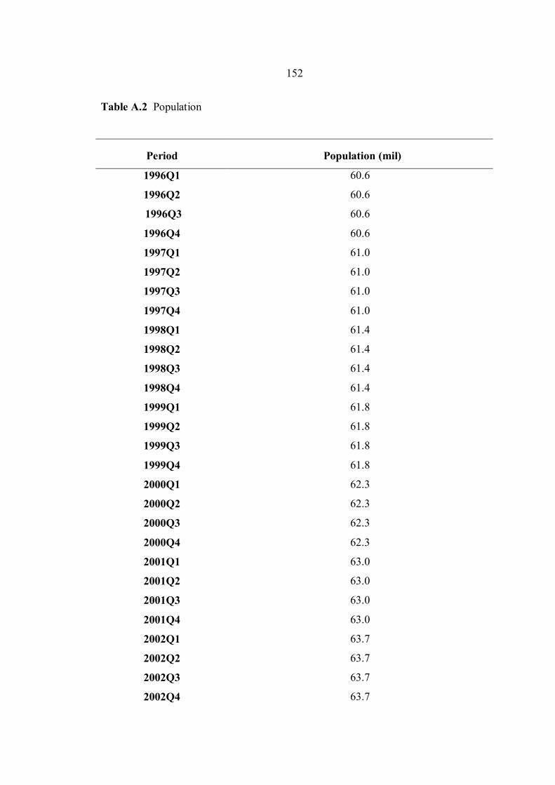
152

Table A.2 Population

Period

Population (mil)

1996Q1

1996Q2

1996Q3

1996Q4

1997Q1

1997Q2

1997Q3

1997Q4

1998Q1

1998Q2

1998Q3

1998Q4

1999Q1

1999Q2

1999Q3

1999Q4

2000Q1

2000Q2

2000Q3

2000Q4

2001Q1

2001Q2

2001Q3

2001Q4

2002Q1

2002Q2

2002Q3

2002Q4

60.6

60.6

60.6

60.6

61.0

61.0

61.0

61.0

61.4

61.4

61.4

61.4

61.8

61.8

61.8

61.8

62.3

62.3

62.3

62.3

63.0

63.0

63.0

63.0

63.7

63.7

63.7

63.7

153

Table A.2 (Continued)

Period

Population (mil)

2003Q1

2003Q2

2003Q3

2003Q4

2004Q1

2004Q2

2004Q3

2004Q4

2005Q1

2005Q2

2005Q3

2005Q4

2006Q1

2006Q2

2006Q3

2006Q4

2007Q1

2007Q2

2007Q3

2007Q4

2008Q1

2008Q2

2008Q3

2008Q4

2009Q1

2009Q2

2009Q3

2009Q4

64.5

64.5

64.5

64.5

65.3

65.3

65.3

65.3

65.9

65.9

65.9

65.9

66.5

66.5

66.5

66.5

67.0

67.0

67.0

67.0

67.4

67.4

67.4

67.4

67.8

67.8

67.8

67.8

154

Table A.2 (Continued)

Period

Population (mil)

2010Q1

2010Q2

2010Q3

2010Q4

67.4

67.4

67.4

67.4

155

Table A.3 Net Government Revenue and Total Tax Revenue and Per Capita Terms

(at Constant Prices)

Period

Net

Government

Revenue (real)

Net Government

Revenue Per

Capita

GREVENUE

Total Tax

Revenue

(Real)

Total Tax

Revenue Per

Capita

TAXREV

1996Q1

1996Q2

1996Q3

1996Q4

1997Q1

1997Q2

1997Q3

1997Q4

1998Q1

1998Q2

1998Q3

1998Q4

1999Q1

1999Q2

1999Q3

1999Q4

2000Q1

2000Q2

2000Q3

2000Q4

2001Q1

2001Q2

2001Q3

2001Q4

139,814

173,458

171,401

114,290

143,803

160,190

138,903

106,491

117,335

121,588

94,719

97,994

111,205

115,318

110,882

103,182

113,457

127,930

115,710

101,005

105,247

135,723

127,042

105,574

2,306

2,861

2,827

1,885

2,357

2,625

2,276

1,745

1,911

1,980

1,543

1,596

1,799

1,865

1,794

1,669

1,820

2,052

1,856

1,620

1,671

2,155

2,017

1,676

123,621

156,926

152,274

115,714

122,914

152,383

139,110

107,500

110,846

115,357

100,774

96,373

114,281

113,938

95,488

98,848

110,858

120,121

110,401

101,509

105,320

130,658

122,545

109,786

2,039

2,589

2,512

1,909

2,014

2,497

2,280

1,762

1,805

1,879

1,641

1,570

1,848

1,843

1,545

1,599

1,778

1,927

1,771

1,628

1,672

2,074

1,945

1,743

156

Table A.3 (Continued)

Period

Net

Government

Revenue (real)

Net Government

Revenue Per

Capita

GREVENUE

Total Tax

Revenue

(Real)

Total Tax

Revenue Per

Capita

TAXREV

2002Q1

2002Q2

2002Q3

2002Q4

2003Q1

2003Q2

2003Q3

2003Q4

2004Q1

2004Q2

2004Q3

2004Q4

2005Q1

2005Q2

2005Q3

2005Q4

2006Q1

2006Q2

2006Q3

2006Q4

2007Q1

2007Q2

2007Q3

2007Q4

2008Q1

120,926

152,844

127,068

121,405

139,327

162,754

144,967

150,630

146,699

181,207

157,905

151,279

158,021

211,177

175,125

142,487

159,988

213,922

179,108

157,016

158,296

215,412

198,317

161,531

152,795

1,897

2,398

1,994

1,905

2,159

2,522

2,247

2,335

2,247

2,776

2,419

2,317

2,396

3,202

2,656

2,161

2,406

3,217

2,693

2,361

2,363

3,216

2,961

2,412

2,267

113,505

146,364

136,988

121,415

131,695

167,858

157,671

141,184

149,634

192,195

178,332

153,260

160,550

215,319

199,755

153,474

160,335

223,665

203,402

160,540

162,274

228,733

203,913

162,754

173,199

1,781

2,296

2,149

1,905

2,041

2,602

2,444

2,188

2,292

2,944

2,732

2,348

2,435

3,265

3,029

2,327

2,411

3,363

3,058

2,414

2,423

3,415

3,044

2,430

2,570

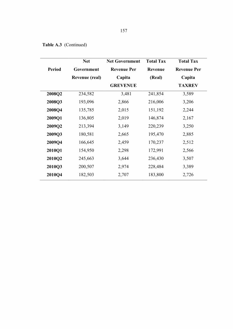
157

Table A.3 (Continued)

Period

Net

Government

Revenue (real)

Net Government

Revenue Per

Capita

GREVENUE

Total Tax

Revenue

(Real)

Total Tax

Revenue Per

Capita

TAXREV

2008Q2

2008Q3

2008Q4

2009Q1

2009Q2

2009Q3

2009Q4

2010Q1

2010Q2

2010Q3

2010Q4

234,582

193,096

135,785

136,805

213,394

180,581

166,645

154,950

245,663

200,507

182,503

3,481

2,866

2,015

2,019

3,149

2,665

2,459

2,298

3,644

2,974

2,707

241,854

216,006

151,192

146,874

220,239

195,470

170,237

172,991

236,430

228,484

183,800

3,589

3,206

2,244

2,167

3,250

2,885

2,512

2,566

3,507

3,389

2,726

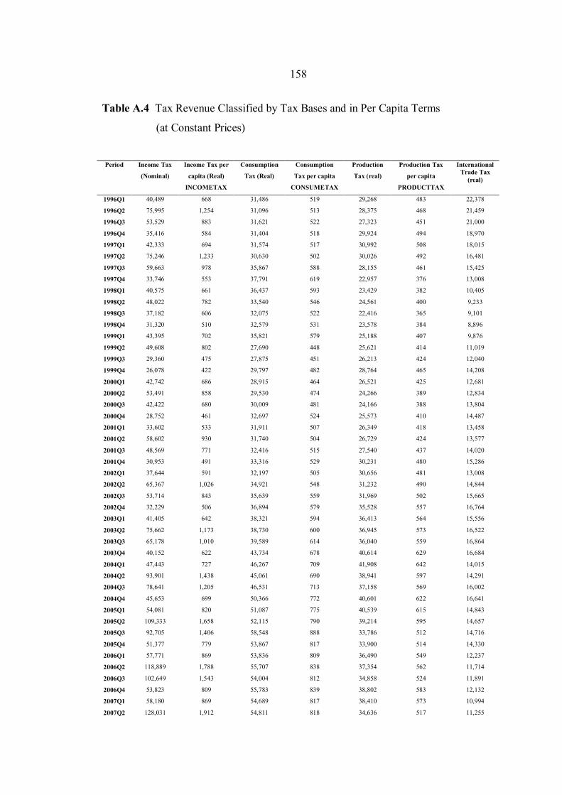
158

Table A.4 Tax Revenue Classified by Tax Bases and in Per Capita Terms

(at Constant Prices)

Period Income Tax

(Nominal)

Income Tax per

capita (Real)

INCOMETAX

Consumption

Tax (Real)

Consumption

Tax per capita

CONSUMETAX

Production

Tax (real)

Production Tax

per capita

PRODUCTTAX

International Trade Tax

(real)

1996Q1

1996Q2

1996Q3

1996Q4

1997Q1

1997Q2

1997Q3

1997Q4

1998Q1

1998Q2

1998Q3

1998Q4

1999Q1

1999Q2

1999Q3

1999Q4

2000Q1

2000Q2

2000Q3

2000Q4

2001Q1

2001Q2

2001Q3

2001Q4

2002Q1

2002Q2

2002Q3

2002Q4

2003Q1

2003Q2

2003Q3

2003Q4

2004Q1

2004Q2

2004Q3

2004Q4

2005Q1

2005Q2

2005Q3

2005Q4

2006Q1

2006Q2

2006Q3

2006Q4

2007Q1

2007Q2

40,489

75,995

53,529

35,416

42,333

75,246

59,663

33,746

40,575

48,022

37,182

31,320

43,395

49,608

29,360

26,078

42,742

53,491

42,422

28,752

33,602

58,602

48,569

30,953

37,644

65,367

53,714

32,229

41,405

75,662

65,178

40,152

47,443

93,901

78,641

45,653

54,081

109,333

92,705

51,377

57,771

118,889

102,649

53,823

58,180

128,031

668

1,254

883

584

694

1,233

978

553

661

782

606

510

702

802

475

422

686

858

680

461

533

930

771

491

591

1,026

843

506

642

1,173

1,010

622

727

1,438

1,205

699

820

1,658

1,406

779

869

1,788

1,543

809

869

1,912

31,486

31,096

31,621

31,404

31,574

30,630

35,867

37,791

36,437

33,540

32,075

32,579

35,821

27,690

27,875

29,797

28,915

29,530

30,009

32,697

31,911

31,740

32,416

33,316

32,197

34,921

35,639

36,894

38,321

38,730

39,589

43,734

46,267

45,061

46,531

50,366

51,087

52,115

58,548

53,867

53,836

55,707

54,004

55,783

54,689

54,811

519

513

522

518

517

502

588

619

593

546

522

531

579

448

451

482

464

474

481

524

507

504

515

529

505

548

559

579

594

600

614

678

709

690

713

772

775

790

888

817

809

838

812

839

817

818

29,268

28,375

27,323

29,924

30,992

30,026

28,155

22,957

23,429

24,561

22,416

23,578

25,188

25,621

26,213

28,764

26,521

24,266

24,166

25,573

26,349

26,729

27,540

30,231

30,656

31,232

31,969

35,528

36,413

36,945

36,040

40,614

41,908

38,941

37,158

40,601

40,539

39,214

33,786

33,900

36,490

37,354

34,858

38,802

38,410

34,636

483

468

451

494

508

492

461

376

382

400

365

384

407

414

424

465

425

389

388

410

418

424

437

480

481

490

502

557

564

573

559

629

642

597

569

622

615

595

512

514

549

562

524

583

573

517

22,378

21,459

21,000

18,970

18,015

16,481

15,425

13,008

10,405

9,233

9,101

8,896

9,876

11,019

12,040

14,208

12,681

12,834

13,804

14,487

13,458

13,577

14,020

15,286

13,008

14,844

15,665

16,764

15,556

16,522

16,864

16,684

14,015

14,291

16,002

16,641

14,843

14,657

14,716

14,330

12,237

11,714

11,891

12,132

10,994

11,255

159

Table A.4 (Continued)

Period Income Tax

(Nominal)

Income Tax per

capita (Real)

INCOMETAX

Consumption

Tax (Real)

Consumption

Tax per capita

CONSUMETAX

Production

Tax (real)

Production Tax

per capita

PRODUCTTAX

International Trade Tax

(real)

2007Q3

2007Q4

2008Q1

2008Q2

2008Q3

2008Q4

2009Q1

2009Q2

2009Q3

2009Q4

2010Q1

2010Q2

2010Q3

2010Q4

104,318

56,719

62,262

136,529

113,227

54,460

58,565

126,660

93,215

52,061

56,384

123,224

115,164

59,275

1,557

847

924

2,026

1,680

808

864

1,869

1,376

768

836

1,828

1,708

879

54,464

58,429

61,758

59,899

62,498

56,815

47,250

48,221

52,681

57,879

57,196

57,376

57,914

61,307

813

872

916

889

927

843

697

712

777

854

848

851

859

909

33,641

35,258

37,128

34,039

28,038

28,066

32,796

37,177

39,702

48,157

49,096

44,548

44,539

51,515

502

526

551

505

416

416

484

549

586

711

728

661

661

764

11,490

12,347

12,051

11,386

12,243

11,850

8,263

8,181

9,872

12,140

10,315

11,282

10,867

11,703

160

Table A.5 Public Expenditure and in Per Capital Terms (at Constant Prices)

Period

Total Government Expenditure

(Real)

Total Government Expenditure

Per Capita (GEXPEND)

1996Q1

1996Q2

1996Q3

1996Q4

1997Q1

1997Q2

1997Q3

1997Q4

1998Q1

1998Q2

1998Q3

1998Q4

1999Q1

1999Q2

1999Q3

1999Q4

2000Q1

2000Q2

2000Q3

2000Q4

2001Q1

2001Q2

2001Q3

2001Q4

2002Q1

2002Q2

2002Q3

124,531

138,019

179,986

140,383

138,784

141,684

194,827

133,054

122,700

110,388

159,900

123,158

110,709

130,819

154,832

120,020

131,533

110,109

146,565

111,358

118,330

119,859

154,031

102,457

120,202

119,055

147,386

2,054

2,277

2,969

2,316

2,274

2,322

3,193

2,180

1,998

1,798

2,604

2,006

1,791

2,116

2,504

1,941

2,110

1,766

2,351

1,786

1,879

1,903

2,445

1,627

1,886

1,868

2,313

161

Table A.5 (Continued)

Period

Total Government Expenditure

(Real)

Total Government Expenditure

Per Capita (GEXPEND)

2002Q4

2003Q1

2003Q2

2003Q3

2003Q4

2004Q1

2004Q2

2004Q3

2004Q4

2005Q1

2005Q2

2005Q3

2005Q4

2006Q1

2006Q2

2006Q3

2006Q4

2007Q1

2007Q2

2007Q3

2007Q4

2008Q1

2008Q2

2008Q3

2008Q4

2009Q1

2009Q2

96,901

106,562

119,716

153,418

109,707

113,530

124,044

154,934

122,888

130,437

139,740

172,633

130,024

135,925

146,340

175,898

129,244

144,225

155,900

190,966

142,150

147,141

151,973

186,964

148,027

147,636

164,463

1,520

1,652

1,855

2,378

1,700

1,739

1,900

2,373

1,882

1,978

2,119

2,618

1,972

2,044

2,200

2,645

1,943

2,153

2,328

2,851

2,122

2,184

2,255

2,775

2,197

2,179

2,427

162

Table A.5 (Continued)

Period

Total Government Expenditure

(Real)

Total Government Expenditure

Per Capita (GEXPEND)

2009Q3

2009Q4

2010Q1

2010Q2

2010Q3

2010Q4

202,933

155,108

161,805

169,859

203,493

155,437

2,995

2,289

2,400

2,519

3,018

2,305

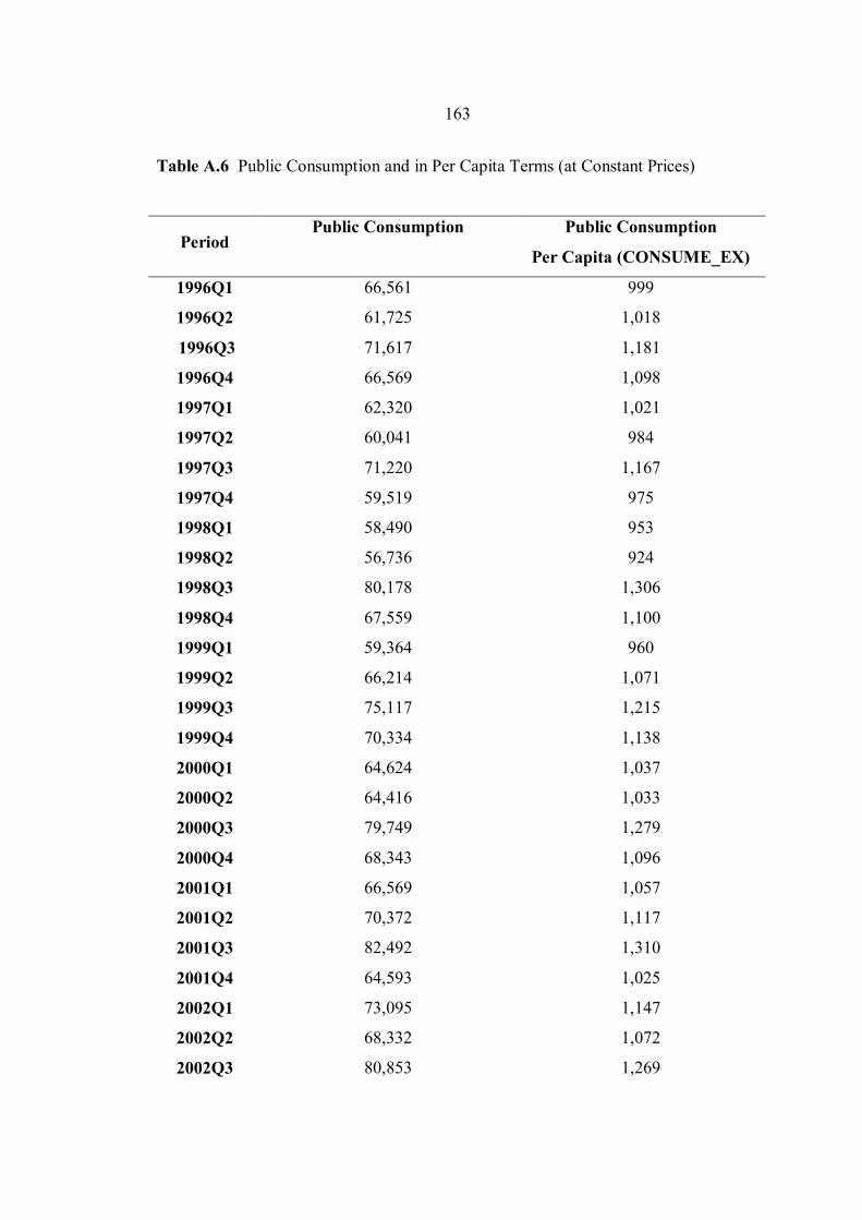
163

Table A.6 Public Consumption and in Per Capita Terms (at Constant Prices)

Period Public Consumption Public Consumption

Per Capita (CONSUME_EX)

1996Q1

1996Q2

1996Q3

1996Q4

1997Q1

1997Q2

1997Q3

1997Q4

1998Q1

1998Q2

1998Q3

1998Q4

1999Q1

1999Q2

1999Q3

1999Q4

2000Q1

2000Q2

2000Q3

2000Q4

2001Q1

2001Q2

2001Q3

2001Q4

2002Q1

2002Q2

2002Q3

66,561

61,725

71,617

66,569

62,320

60,041

71,220

59,519

58,490

56,736

80,178

67,559

59,364

66,214

75,117

70,334

64,624

64,416

79,749

68,343

66,569

70,372

82,492

64,593

73,095

68,332

80,853

999

1,018

1,181

1,098

1,021

984

1,167

975

953

924

1,306

1,100

960

1,071

1,215

1,138

1,037

1,033

1,279

1,096

1,057

1,117

1,310

1,025

1,147

1,072

1,269

164

Table A.6 (Continued)

Period Public Consumption Public Consumption

Per Capita (CONSUME_EX)

2002Q4

2003Q1

2003Q2

2003Q3

2003Q4

2004Q1

2004Q2

2004Q3

2004Q4

2005Q1

2005Q2

2005Q3

2005Q4

2006Q1

2006Q2

2006Q3

2006Q4

2007Q1

2007Q2

2007Q3

2007Q4

2008Q1

2008Q2

2008Q3

2008Q4

2009Q1

2009Q2

63,778

67,174

71,976

85,049

68,894

72,497

76,487

86,173

74,726

80,404

83,278

101,896

79,345

83,790

87,191

103,760

77,772

91,108

95,210

114,350

86,230

91,962

93,668

116,252

97,432

97,563

101,028

1,001

1,041

1,116

1,318

1,068

1,111

1,172

1,320

1,145

1,219

1,263

1,545

1,203

1,260

1,311

1,560

1,169

1,360

1,421

1,707

1,287

1,365

1,390

1,725

1,446

1,440

1,491

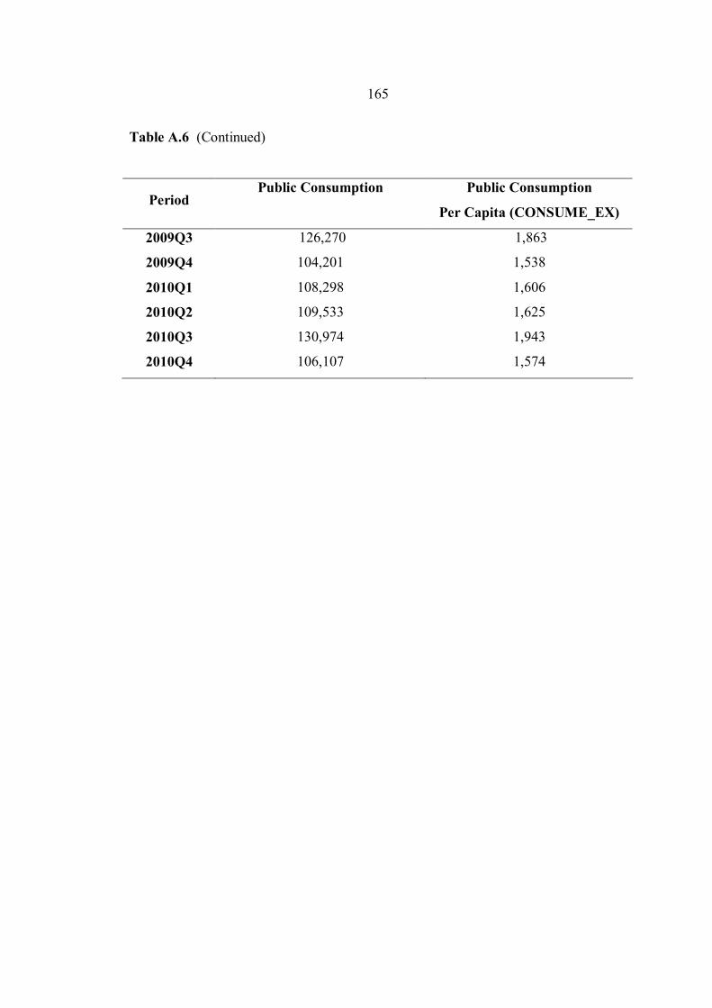
165

Table A.6 (Continued)

Period Public Consumption Public Consumption

Per Capita (CONSUME_EX)

2009Q3

2009Q4

2010Q1

2010Q2

2010Q3

2010Q4

126,270

104,201

108,298

109,533

130,974

106,107

1,863

1,538

1,606

1,625

1,943

1,574

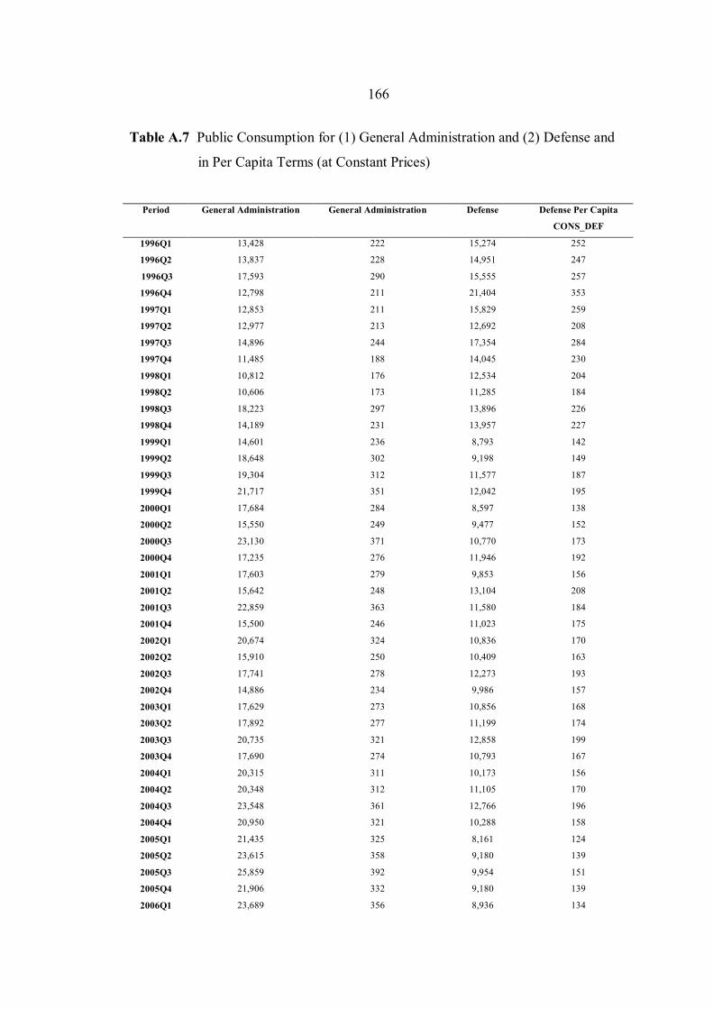
166

Table A.7 Public Consumption for (1) General Administration and (2) Defense and

in Per Capita Terms (at Constant Prices)

Period General Administration General Administration Defense Defense Per Capita

CONS_DEF

1996Q1

1996Q2

1996Q3

1996Q4

1997Q1

1997Q2

1997Q3

1997Q4

1998Q1

1998Q2

1998Q3

1998Q4

1999Q1

1999Q2

1999Q3

1999Q4

2000Q1

2000Q2

2000Q3

2000Q4

2001Q1

2001Q2

2001Q3

2001Q4

2002Q1

2002Q2

2002Q3

2002Q4

2003Q1

2003Q2

2003Q3

2003Q4

2004Q1

2004Q2

2004Q3

2004Q4

2005Q1

2005Q2

2005Q3

2005Q4

2006Q1

13,428

13,837

17,593

12,798

12,853

12,977

14,896

11,485

10,812

10,606

18,223

14,189

14,601

18,648

19,304

21,717

17,684

15,550

23,130

17,235

17,603

15,642

22,859

15,500

20,674

15,910

17,741

14,886

17,629

17,892

20,735

17,690

20,315

20,348

23,548

20,950

21,435

23,615

25,859

21,906

23,689

222

228

290

211

211

213

244

188

176

173

297

231

236

302

312

351

284

249

371

276

279

248

363

246

324

250

278

234

273

277

321

274

311

312

361

321

325

358

392

332

356

15,274

14,951

15,555

21,404

15,829

12,692

17,354

14,045

12,534

11,285

13,896

13,957

8,793

9,198

11,577

12,042

8,597

9,477

10,770

11,946

9,853

13,104

11,580

11,023

10,836

10,409

12,273

9,986

10,856

11,199

12,858

10,793

10,173

11,105

12,766

10,288

8,161

9,180

9,954

9,180

8,936

252

247

257

353

259

208

284

230

204

184

226

227

142

149

187

195

138

152

173

192

156

208

184

175

170

163

193

157

168

174

199

167

156

170

196

158

124

139

151

139

134

167

Table A.7 (Continued)

Period General Administration General Administration Defense Defense Per Capita

CONS_DEF

2006Q2

2006Q3

2006Q4

2007Q1

2007Q2

2007Q3

2007Q4

2008Q1

2008Q2

2008Q3

2008Q4

2009Q1

2009Q2

2009Q3

2009Q4

2010Q1

2010Q2

2010Q3

2010Q4

24,009

29,401

20,155

23,892

24,422

30,421

22,089

24,957

25,758

34,032

23,530

25,016

26,366

34,706

27,997

30,332

31,883

40,005

29,012

361

442

303

357

365

454

330

370

382

505

349

369

389

512

413

450

473

593

430

9,365

9,607

9,149

8,749

10,605

12,790

9,764

9,708

10,781

12,763

11,325

9,949

12,081

14,935

11,950

10,918

12,214

14,765

12,165

141

144

138

131

158

191

146

144

160

189

168

147

178

220

176

162

181

219

180

168

Table A.8 Public Consumption for (3) Justice and Police and (4) Education and

Research and in Per Capita Terms (at Constant Prices)

Period Justice and Police Justice and Police Per Capita

CONS_JUST

Education and

Research

Education and

Research Per Capita

CONS_EDU

1996Q1

1996Q2

1996Q3

1996Q4

1997Q1

1997Q2

1997Q3

1997Q4

1998Q1

1998Q2

1998Q3

1998Q4

1999Q1

1999Q2

1999Q3

1999Q4

2000Q1

2000Q2

2000Q3

2000Q4

2001Q1

2001Q2

2001Q3

2001Q4

2002Q1

2002Q2

2002Q3

2002Q4

2003Q1

2003Q2

2003Q3

2003Q4

2004Q1

2004Q2

2004Q3

2004Q4

2005Q1

2005Q2

2005Q3

2005Q4

5,606

5,925

6,502

5,481

5,858

5,729

6,332

5,499

5,590

5,693

6,545

6,091

5,539

5,992

6,598

5,795

5,904

6,298

7,147

6,399

6,597

7,550

8,020

6,523

6,869

6,934

7,803

6,994

7,259

7,473

8,354

7,422

7,296

7,905

9,246

8,487

9,922

9,709

12,279

9,185

92

98

107

90

96

94

104

90

91

93

107

99

90

97

107

94

95

101

115

103

105

120

127

104

108

109

122

110

112

116

129

115

112

121

142

130

150

147

186

139

17,097

17,469

20,508

17,908

17,882

18,907

20,761

18,176

19,715

19,974

26,287

23,445

20,027

21,419

23,828

20,748

21,574

22,385

25,358

23,015

21,409

22,541

25,568

21,877

23,010

23,201

26,216

22,057

22,232

25,303

29,456

24,033

24,290

25,908

26,962

25,742

26,960

25,469

30,264

24,786

282

288

338

295

293

310

340

298

321

325

428

382

324

346

385

336

346

359

407

369

340

358

406

347

361

364

411

346

345

392

457

372

372

397

413

394

409

386

459

376

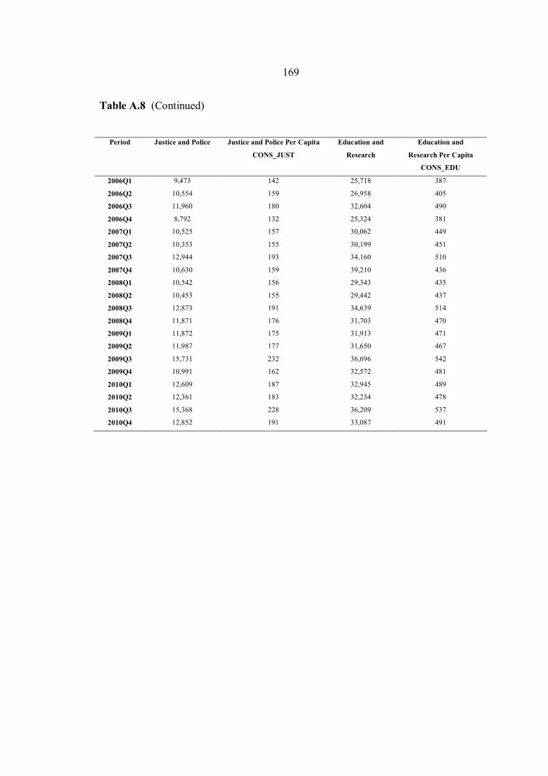
169

Table A.8 (Continued)

Period Justice and Police Justice and Police Per Capita

CONS_JUST

Education and

Research

Education and

Research Per Capita

CONS_EDU

2006Q1

2006Q2

2006Q3

2006Q4

2007Q1

2007Q2

2007Q3

2007Q4

2008Q1

2008Q2

2008Q3

2008Q4

2009Q1

2009Q2

2009Q3

2009Q4

2010Q1

2010Q2

2010Q3

2010Q4

9,473

10,554

11,960

8,792

10,525

10,353

12,944

10,630

10,542

10,453

12,873

11,871

11,872

11,987

15,731

10,991

12,609

12,361

15,368

12,852

142

159

180

132

157

155

193

159

156

155

191

176

175

177

232

162

187

183

228

191

25,718

26,958

32,604

25,324

30,062

30,199

34,160

39,210

29,343

29,442

34,639

31,703

31,913

31,650

36,696

32,572

32,945

32,234

36,209

33,087

387

405

490

381

449

451

510

436

435

437

514

470

471

467

542

481

489

478

537

491

170

Table A.9 Public Consumption for (5) Health Services and (6) Special Welfare

Services and in Per Capita Terms (at Constant Prices)

Period Health Services Health Services Per Capita

CONS_HEALTH

Special Welfare

Services

Special Welfare

Services Per Capita

CONS_WELFARE

1996Q1

1996Q2

1996Q3

1996Q4

1997Q1

1997Q2

1997Q3

1997Q4

1998Q1

1998Q2

1998Q3

1998Q4

1999Q1

1999Q2

1999Q3

1999Q4

2000Q1

2000Q2

2000Q3

2000Q4

2001Q1

2001Q2

2001Q3

2001Q4

2002Q1

2002Q2

2002Q3

2002Q4

2003Q1

2003Q2

2003Q3

2003Q4

2004Q1

2004Q2

2004Q3

2004Q4

2005Q1

2005Q2

2005Q3

2005Q4

5,530

5,826

7,102

5,447

6,639

6,384

7,750

7,347

6,795

6,154

10,833

6,870

7,098

7,374

8,921

6,914

7,550

7,462

8,969

7,099

8,058

8,392

10,063

7,123

7,317

7,410

11,182

6,075

6,258

6,676

9,215

6,169

6,729

7,304

8,277

6,271

8,966

9,345

11,125

7,881

91

96

117

90

109

105

127

120

111

100

176

112

115

119

144

112

121

120

144

114

128

133

160

113

115

116

175

95

97

103

143

96

103

112

127

96

136

142

169

120

498

506

600

503

540

519

620

470

431

423

677

451

460

661

936

468

554

583

721

496

511

527

706

469

555

515

672

904

553

762

995

654

740

818

978

699

492

598

1,084

1,066

8

8

10

8

9

9

10

8

7

7

11

7

7

11

15

8

9

9

12

8

8

8

11

7

9

8

11

14

9

12

15

10

11

13

15

11

7

9

16

16

171

Table A.9 (Continued)

Period Health Services Health Services Per Capita

CONS_HEALTH

Special Welfare

Services

Special Welfare

Services Per Capita

CONS_WELFARE

2006Q1

2006Q2

2006Q3

2006Q4

2007Q1

2007Q2

2007Q3

2007Q4

2008Q1

2008Q2

2008Q3

2008Q4

2009Q1

2009Q2

2009Q3

2009Q4

2010Q1

2010Q2

2010Q3

2010Q4

9,126

9,525

10,042

7,929

10,145

10,506

12,079

8,595

9,810

9,709

11,080

11,928

10,318

10,188

12,895

10,175

10,648

10,358

11,781

10,742

137

143

151

119

151

157

180

128

146

144

164

177

152

150

190

150

158

154

175

159

1,018

1,194

1,444

892

1,534

1,583

2,026

1,107

1,435

1,418

2,033

1,671

1,616

1,667

2,456

1,676

1,881

1,956

2,804

1,839

15

18

22

13

23

24

30

17

21

21

30

25

24

25

36

25

28

29

42

27

172

Table A.10 Public Consumption for (7) Transport and Communication Facilities and

(8) Other Services and in Per Capita Terms (at Constant Prices)

Period Transport and

Communication

Facilities

Transport and

Communication Facilities Per Capita

CONS_TRANSPORT

Other Services Other Services

Per Capita

CONS_OTHER

1996Q1

1996Q2

1996Q3

1996Q4

1997Q1

1997Q2

1997Q3

1997Q4

1998Q1

1998Q2

1998Q3

1998Q4

1999Q1

1999Q2

1999Q3

1999Q4

2000Q1

2000Q2

2000Q3

2000Q4

2001Q1

2001Q2

2001Q3

2001Q4

2002Q1

2002Q2

2002Q3

2002Q4

2003Q1

2003Q2

2003Q3

2003Q4

2004Q1

2004Q2

2004Q3

2004Q4

2005Q1

2005Q2

2005Q3

2005Q4

1,156

1,310

1,548

1,133

1,163

1,230

1,465

1,083

1,112

1,160

1,634

1,196

1,430

1,400

1,901

1,297

1,212

1,079

1,389

1,012

1,215

1,158

1,479

1,052

2,233

2,273

2,304

1,343

960

932

1,209

827

1,239

1,318

1,786

1,039

2,248

3,224

8,231

3,603

19

22

26

19

19

20

24

18

18

19

27

19

23

23

31

21

19

17

22

16

19

18

23

17

35

36

36

21

15

14

19

13

19

20

27

16

34

49

125

55

1,972

1,900

2,208

1,895

1,556

1,601

2,042

1,414

1,500

1,441

2,082

1,359

1,417

1,523

2,051

1,354

1,550

1,581

2,264

1,142

1,323

1,459

2,217

1,027

1,601

1,679

2,661

1,534

1,428

1,738

2,226

1,306

1,716

1,782

2,611

1,250

2,220

2,138

3,100

1,739

33

31

36

31

26

26

33

23

24

23

34

22

23

25

33

22

25

25

36

18

21

23

35

16

25

26

42

24

22

27

34

20

26

27

40

19

34

32

47

26

173

Table A.10 (Continued)

Period Health Services Health Services Per Capita

CONS_HEALTH

Special Welfare

Services

Special Welfare

Services Per Capita

CONS_WELFARE

2006Q1

2006Q2

2006Q3

2006Q4

2007Q1

2007Q2

2007Q3

2007Q4

2008Q1

2008Q2

2008Q3

2008Q4

2009Q1

2009Q2

2009Q3

2009Q4

2010Q1

2010Q2

2010Q3

2010Q4

3,701

3,374

5,667

3,505

3,774

5,208

6,952

2,687

3,567

3,759

5,121

2,785

4,009

4,331

5,139

5,807

5,768

5,228

5,585

3,321

56

51

85

53

56

78

104

40

53

56

76

41

59

64

76

86

86

78

83

49

2,129

2,211

3,036

2,027

2,428

2,335

2,978

2,148

2,600

2,348

3,711

2,620

2,871

2,759

3,713

3,033

3,195

3,300

4,457

3,088

32

33

46

30

36

35

44

32

39

35

55

39

42

41

55

45

47

49

66

46

174

Table A.11 Public Investment and in Per Capita Terms (at Constant Prices)

Period Public

Investment

Public

Investment

Per Capita

INVEST_EX

Construction Construction

Per Capita

INV_CON

Equipment Equipment

Per Capita

INV_EQM

1996Q1

1996Q2

1996Q3

1996Q4

1997Q1

1997Q2

1997Q3

1997Q4

1998Q1

1998Q2

1998Q3

1998Q4

1999Q1

1999Q2

1999Q3

1999Q4

2000Q1

2000Q2

2000Q3

2000Q4

2001Q1

2001Q2

2001Q3

2001Q4

2002Q1

2002Q2

2002Q3

2002Q4

2003Q1

2003Q2

2003Q3

2003Q4

2004Q1

2004Q2

2004Q3

2004Q4

2005Q1

2005Q2

2005Q3

2005Q4

63,970

76,294

108,369

73,814

76,464

81,643

123,607

73,535

64,210

53,652

79,722

55,599

51,345

64,605

79,715

49,686

66,909

45,693

66,816

43,015

51,761

49,486

71,539

37,864

47,107

50,723

66,533

33,123

39,388

47,740

68,369

40,813

41,033

47,557

68,761

48,162

50,033

56,462

70,737

50,679

1,055

1,259

1,788

1,218

1,253

1,338

2,026

1,205

1,046

874

1,298

906

831

1,045

1,289

804

1,073

733

1,072

690

822

786

1,136

601

739

796

1,044

520

610

740

1,060

633

629

729

1,053

738

759

856

1,073

768

53,164

58,387

76,188

57,500

56,567

65,887

98,457

52,883

47,902

43,733

64,941

41,748

39,868

49,076

61,297

38,012

42,553

35,701

48,386

24,545

37,648

31,343

52,583

26,597

34,540

35,722

46,580

22,195

29,276

33,710

48,002

23,143

29,737

32,657

48,196

28,857

33,872

35,763

49,393

28,962

877

963

1,257

949

927

1,080

1,613

867

780

712

1,058

680

645

794

991

615

683

573

776

394

598

498

835

422

542

560

731

348

454

522

744

359

456

500

738

442

514

542

749

439

10,806

17,907

32,181

16,314

19,897

15,756

25,150

20,652

16,308

9,919

14,781

13,851

11,477

15,529

18,418

11,674

24,356

9,992

18,430

18,470

14,113

18,143

18,956

11,267

12,567

15,001

19,953

10,928

10,112

14,030

20,367

17,670

11,296

14,900

20,565

19,305

16,161

20,699

21,344

21,717

178

295

531

269

326

258

412

338

266

162

241

226

186

251

298

189

391

160

296

296

224

288

301

179

197

235

313

171

157

217

316

274

173

228

315

296

245

314

324

329

175

Table A.11 (Continued)

Period Public

Investment

Public

Investment

Per Capita

INVEST_EX

Construction Construction

Per Capita

INV_CON

Equipment Equipment

Per Capita

INV_EQM

2006Q1

2006Q2

2006Q3

2006Q4

2007Q1

2007Q2

2007Q3

2007Q4

2008Q1

2008Q2

2008Q3

2008Q4

2009Q1

2009Q2

2009Q3

2009Q4

2010Q1

2010Q2

2010Q3

2010Q4

52,135

59,149

72,138

51,472

53,117

60,690

76,616

55,920

55,179

58,305

70,712

50,595

50,073

63,435

76,663

50,907

53,507

60,326

72,519

49,330

784

889

1,085

774

793

906

1,144

835

819

865

1,049

751

739

936

1,131

751

794

895

1,076

732

36,009

38,784

52,251

30,823

36,348

40,397

52,793

39,311

37,558

38,106

47,767

30,153

34,663

42,319

52,763

32,879

36,081

44,799

52,797

34,070

541

583

786

463

543

603

788

587

557

565

709

447

512

625

779

485

535

664

783

505

16,126

20,365

19,887

20,649

16,769

20,293

23,823

16,609

17,621

20,199

22,945

20,442

15,410

21,116

23,900

18,028

17,426

15,527

19,722

15,260

242

306

299

310

250

303

356

248

261

300

341

303

227

312

353

266

258

230

293

266

BIOGRAPHY

NAME Pisit Puapan

ACADEMIC BACKGROUND B.A. (Economics), Boston College, USA, 1997

M.A. (International Economics and Finance),

Brandeis University, USA, 2001

PRESENT POSITION Director of Macroeconomic Analysis Division,

Bureau of Macroeconomic Policy, Fiscal Policy

Office

EXPERIENCES Fiscal Policy Office, Ministry of Finance,

Thailand, 1998-present