the excel sheet providing the necessary inputs for the ... · the possible formation of one solid...
TRANSCRIPT
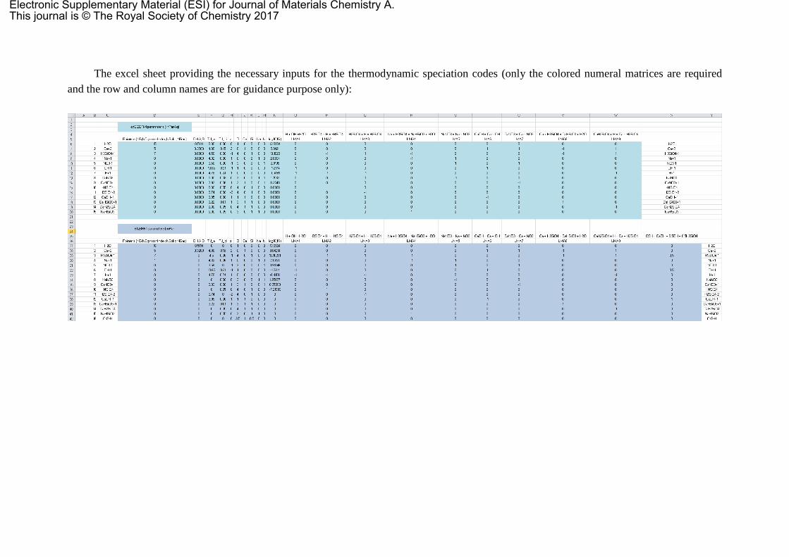
The excel sheet providing the necessary inputs for the thermodynamic speciation codes (only the colored numeral matrices are required
and the row and column names are for guidance purpose only):
Electronic Supplementary Material (ESI) for Journal of Materials Chemistry A.This journal is © The Royal Society of Chemistry 2017
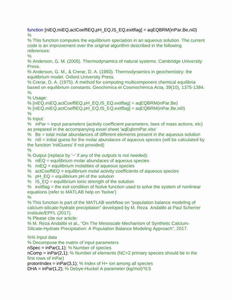
function [niEQ,miEQ,actCoeffiEQ,pH_EQ,IS_EQ,exitflag] = aqEQBRM(inPar,Be,ni0)
% % This function computes the equilibrium speciation in an aqueous solution. The current code is an improvement over the original algorithm described in the following references: % % Anderson, G. M. (2005). Thermodynamics of natural systems. Cambridge University Press. % Anderson, G. M., & Crerar, D. A. (1993). Thermodynamics in geochemistry: the equilibrium model. Oxford University Press.
% Crerar, D. A. (1975). A method for computing multicomponent chemical equilibria based on equilibrium constants. Geochimica et Cosmochimica Acta, 39(10), 1375-1384. % % Usage: % [niEQ,miEQ,actCoeffiEQ,pH_EQ,IS_EQ,exitflag] = aqEQBRM(inPar,Be)
% [niEQ,miEQ,actCoeffiEQ,pH_EQ,IS_EQ,exitflag] = aqEQBRM(inPar,Be,ni0)
% % Input: % inPar = input parameters (activity coefficient parameters, laws of mass actions, etc) as prepared in the accompanying excel sheet 'aqEqbrmPar.xlsx' % Be = total molar abundances of different elements present in the aqueous solution
% ni0 = initial guess for the molar abundaces of aqueous species (will be calculated by the function 'initGuess' if not provided)
% % Output (replace by '~' if any of the outputs is not needed): % niEQ = equilibrium molar abundaces of aqueous species
% miEQ = equilibrium molalities of aqueous species
% actCoeffiEQ = equilibrium molal activity coefficients of aqueous species
% pH_EQ = equilibrium pH of the solution
% IS_EQ = equilibrium ionic strength of the solution
% exitflag = the exit condition of fsolve function used to solve the system of nonlinear equations (refer to MATLAB help on 'fsolve')
% % This function is part of the MATLAB workflow on "population balance modeling of calcium-silicate-hydrate precipitaion" developed by M. Reza Andalibi at Paul Scherrer Institute/EPFL (2017). % Please cite our article: % M. Reza Andalibi et al., "On The Mesoscale Mechanism of Synthetic Calcium-Silicate-Hydrate Precipitation: A Population Balance Modeling Approach", 2017. %% Input data
% Decompose the matrix of input parameters
nSpec = inPar(1,1); % Number of species
nComp = inPar(2,1); % Number of elements (NC+2 primary species should be in the first rows of inPar)
protonIndex = inPar(3,1); % Index of H+ ion among all species
DHA = inPar(1,2); % Debye-Huckel A parameter (kg/mol)^0.5
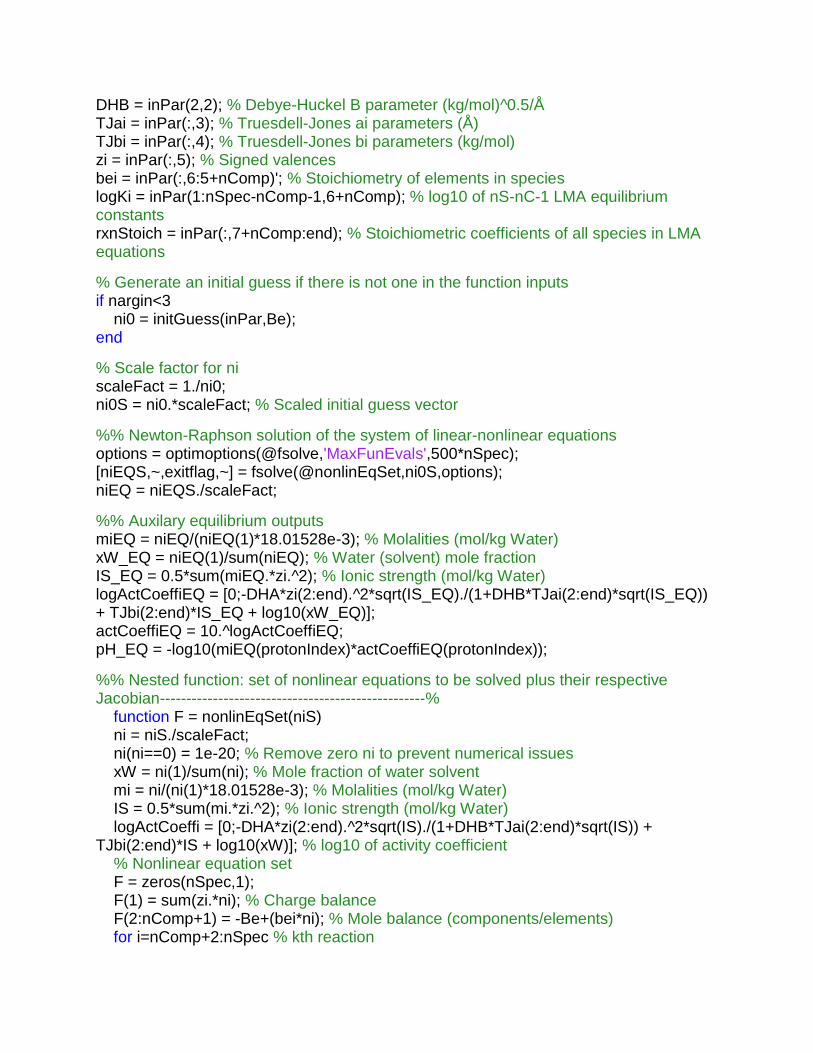
DHB = inPar(2,2); % Debye-Huckel B parameter (kg/mol)^0.5/Å
TJai = inPar(:,3); % Truesdell-Jones ai parameters (Å)
TJbi = inPar(:,4); % Truesdell-Jones bi parameters (kg/mol)
zi = inPar(:,5); % Signed valences
bei = inPar(:,6:5+nComp)'; % Stoichiometry of elements in species
logKi = inPar(1:nSpec-nComp-1,6+nComp); % log10 of nS-nC-1 LMA equilibrium constants
rxnStoich = inPar(:,7+nComp:end); % Stoichiometric coefficients of all species in LMA equations % Generate an initial guess if there is not one in the function inputs
if nargin<3
ni0 = initGuess(inPar,Be); end
% Scale factor for ni scaleFact = 1./ni0; ni0S = ni0.*scaleFact; % Scaled initial guess vector
%% Newton-Raphson solution of the system of linear-nonlinear equations
options = optimoptions(@fsolve,'MaxFunEvals',500*nSpec); [niEQS,~,exitflag,~] = fsolve(@nonlinEqSet,ni0S,options); niEQ = niEQS./scaleFact; %% Auxilary equilibrium outputs
miEQ = niEQ/(niEQ(1)*18.01528e-3); % Molalities (mol/kg Water)
xW_EQ = niEQ(1)/sum(niEQ); % Water (solvent) mole fraction
IS_EQ = 0.5*sum(miEQ.*zi.^2); % Ionic strength (mol/kg Water)
logActCoeffiEQ = [0;-DHA*zi(2:end).^2*sqrt(IS_EQ)./(1+DHB*TJai(2:end)*sqrt(IS_EQ)) + TJbi(2:end)*IS_EQ + log10(xW_EQ)]; actCoeffiEQ = 10.^logActCoeffiEQ; pH_EQ = -log10(miEQ(protonIndex)*actCoeffiEQ(protonIndex));
%% Nested function: set of nonlinear equations to be solved plus their respective Jacobian--------------------------------------------------%
function F = nonlinEqSet(niS)
ni = niS./scaleFact; ni(ni==0) = 1e-20; % Remove zero ni to prevent numerical issues
xW = ni(1)/sum(ni); % Mole fraction of water solvent mi = ni/(ni(1)*18.01528e-3); % Molalities (mol/kg Water)
IS = 0.5*sum(mi.*zi.^2); % Ionic strength (mol/kg Water)
logActCoeffi = [0;-DHA*zi(2:end).^2*sqrt(IS)./(1+DHB*TJai(2:end)*sqrt(IS)) + TJbi(2:end)*IS + log10(xW)]; % log10 of activity coefficient % Nonlinear equation set F = zeros(nSpec,1); F(1) = sum(zi.*ni); % Charge balance
F(2:nComp+1) = -Be+(bei*ni); % Mole balance (components/elements)
for i=nComp+2:nSpec % kth reaction
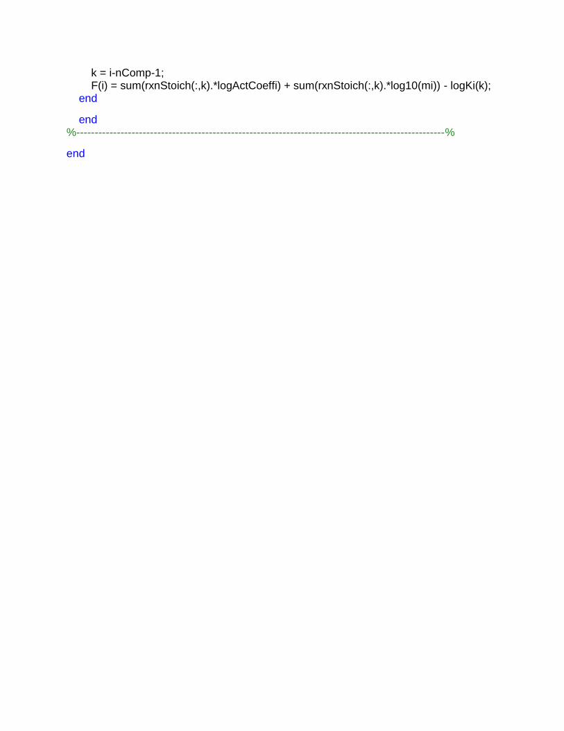
k = i-nComp-1; F(i) = sum(rxnStoich(:,k).*logActCoeffi) + sum(rxnStoich(:,k).*log10(mi)) - logKi(k); end
end
%----------------------------------------------------------------------------------------------------%
end
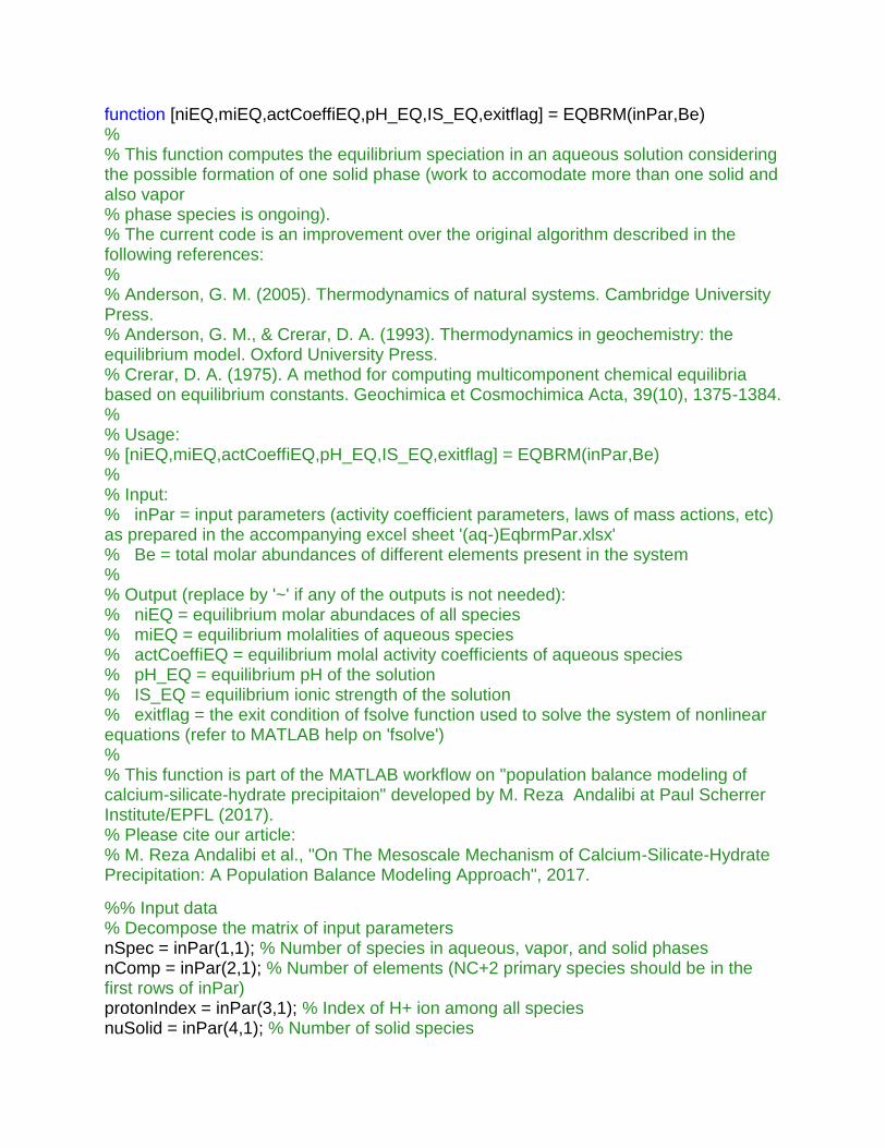
function [niEQ,miEQ,actCoeffiEQ,pH_EQ,IS_EQ,exitflag] = EQBRM(inPar,Be)
% % This function computes the equilibrium speciation in an aqueous solution considering the possible formation of one solid phase (work to accomodate more than one solid and also vapor
% phase species is ongoing). % The current code is an improvement over the original algorithm described in the following references: % % Anderson, G. M. (2005). Thermodynamics of natural systems. Cambridge University Press. % Anderson, G. M., & Crerar, D. A. (1993). Thermodynamics in geochemistry: the equilibrium model. Oxford University Press. % Crerar, D. A. (1975). A method for computing multicomponent chemical equilibria based on equilibrium constants. Geochimica et Cosmochimica Acta, 39(10), 1375-1384. % % Usage: % [niEQ,miEQ,actCoeffiEQ,pH_EQ,IS_EQ,exitflag] = EQBRM(inPar,Be)
% % Input: % inPar = input parameters (activity coefficient parameters, laws of mass actions, etc) as prepared in the accompanying excel sheet '(aq-)EqbrmPar.xlsx' % Be = total molar abundances of different elements present in the system
% % Output (replace by '~' if any of the outputs is not needed): % niEQ = equilibrium molar abundaces of all species
% miEQ = equilibrium molalities of aqueous species
% actCoeffiEQ = equilibrium molal activity coefficients of aqueous species
% pH_EQ = equilibrium pH of the solution
% IS_EQ = equilibrium ionic strength of the solution
% exitflag = the exit condition of fsolve function used to solve the system of nonlinear equations (refer to MATLAB help on 'fsolve')
% % This function is part of the MATLAB workflow on "population balance modeling of calcium-silicate-hydrate precipitaion" developed by M. Reza Andalibi at Paul Scherrer Institute/EPFL (2017). % Please cite our article: % M. Reza Andalibi et al., "On The Mesoscale Mechanism of Calcium-Silicate-Hydrate Precipitation: A Population Balance Modeling Approach", 2017. %% Input data
% Decompose the matrix of input parameters
nSpec = inPar(1,1); % Number of species in aqueous, vapor, and solid phases
nComp = inPar(2,1); % Number of elements (NC+2 primary species should be in the first rows of inPar)
protonIndex = inPar(3,1); % Index of H+ ion among all species
nuSolid = inPar(4,1); % Number of solid species

nuVap = inPar(5,1); % Number of species in vapor phase
nuAq = nSpec-nuSolid-nuVap; % Number of aqueous species
DHA = inPar(1,2); % Debye-Huckel A parameter (kg/mol)^0.5
DHB = inPar(2,2); % Debye-Huckel B parameter (kg/mol)^0.5/Å
TJai = inPar(1:nuAq,3); % Truesdell-Jones ai parameters (Å)
TJbi = inPar(1:nuAq,4); % Truesdell-Jones bi parameters (kg/mol)
zi = inPar(1:nuAq,5); % Signed valences
bei = inPar(:,6:5+nComp)'; % Stoichiometry of elements in species
logKi = inPar(1:nSpec-nComp-1,6+nComp); % log10 of nS-nC-1 LMA equilibrium constants
rxnStoich = inPar(:,7+nComp:end); % Stoichiometric coefficients of all species in LMA equations
%% Initial guess generation
% Aqueous equilibrium calculation
% Deriving inParAq from inPar
inParAq = inPar(1:nuAq,1:end-nuSolid-nuVap); inParAq(1,1) = nuAq; inParAq(4:end,1) = 0; inParAq(nuAq-nComp:end,6+nComp) = 0; [niAQ,miAQ,actCoeffiAQ,pH_AQ,IS_AQ,exitflag] = aqEQBRM(inParAq,Be);
ni0 = [niAQ;zeros(nuSolid,1)]; % Initial guess if system is not much supersaturated
% Saturation index check and possibly re-calculations considering SLE
SI = zeros(nuSolid,1); % Saturation index
for i=1:nuSolid
SI(i,1) = sum(rxnStoich(1:nuAq,end-nuSolid-nuVap+i).*log10(miAQ))... + sum(rxnStoich(1:nuAq,end-nuSolid-nuVap+i).*log10(actCoeffiAQ)) - logKi(end-nuSolid-nuVap+i,1); end
[maxSI,maxSI_index] = max(SI); if maxSI <=0 % (under-)saturated system
niEQ = [niAQ;0]; % Zero mole amount for undersaturated solid
miEQ = miAQ; actCoeffiEQ = actCoeffiAQ; pH_EQ = pH_AQ; IS_EQ = IS_AQ; elseif (0<maxSI) && (maxSI<=0.1) % Slightly supersaturated system
ni0(maxSI_index+nuAq) = 0; % Initial guess for solid mole amount % Newton-Raphson solution using the generated initial guess (SLE)
alphaS = 1./ni0; alphaS(alphaS==Inf) = 1; % Correcting for division by zero
ni0S = ni0.*alphaS; options = optimoptions(@fsolve,'MaxFunEvals',1000*nSpec,'MaxIter',500); [niEQscaled,~,exitflag,~] = fsolve(@nonlinEqSet,ni0S,options); niEQ = niEQscaled./alphaS; % Auxilary equilibrium outputs
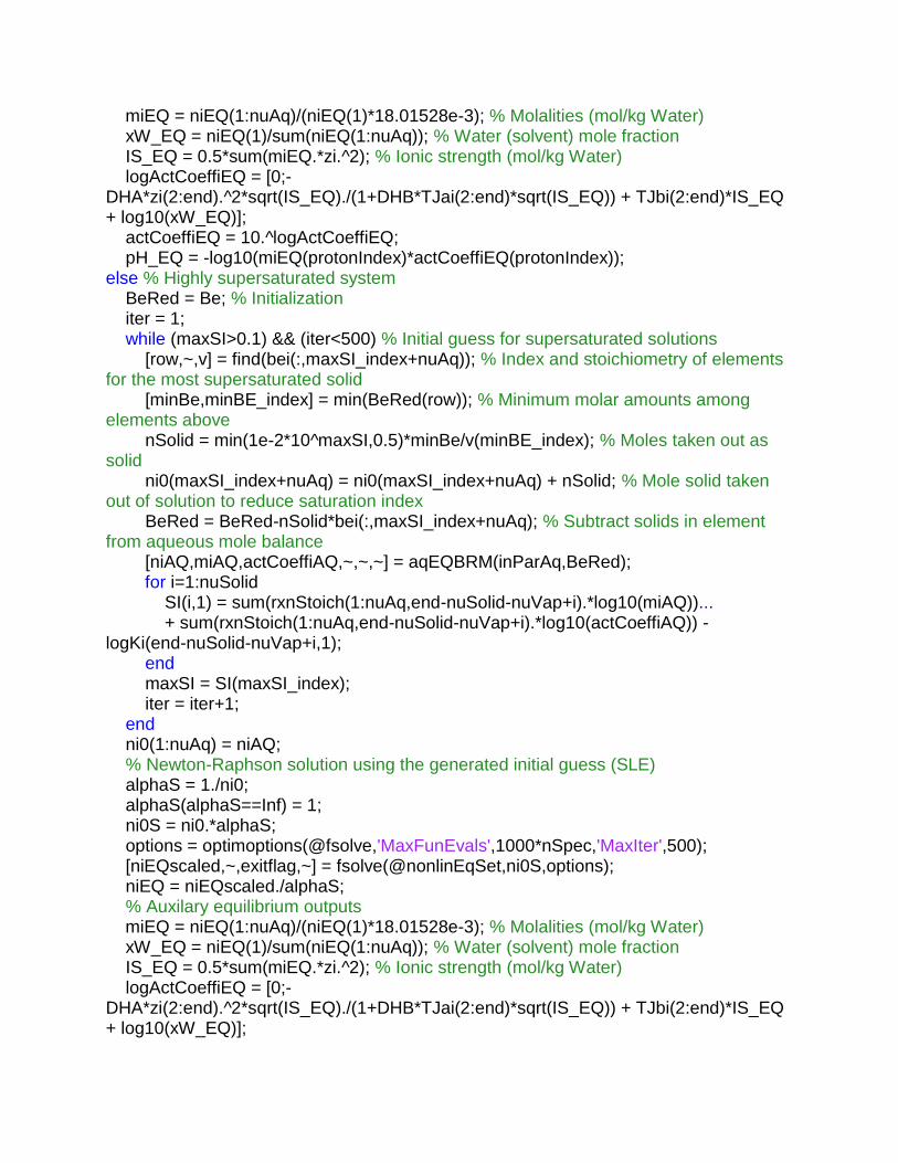
miEQ = niEQ(1:nuAq)/(niEQ(1)*18.01528e-3); % Molalities (mol/kg Water)
xW_EQ = niEQ(1)/sum(niEQ(1:nuAq)); % Water (solvent) mole fraction
IS_EQ = 0.5*sum(miEQ.*zi.^2); % Ionic strength (mol/kg Water)
logActCoeffiEQ = [0;-DHA*zi(2:end).^2*sqrt(IS_EQ)./(1+DHB*TJai(2:end)*sqrt(IS_EQ)) + TJbi(2:end)*IS_EQ + log10(xW_EQ)]; actCoeffiEQ = 10.^logActCoeffiEQ; pH_EQ = -log10(miEQ(protonIndex)*actCoeffiEQ(protonIndex)); else % Highly supersaturated system
BeRed = Be; % Initialization
iter = 1; while (maxSI>0.1) && (iter<500) % Initial guess for supersaturated solutions
[row,~,v] = find(bei(:,maxSI_index+nuAq)); % Index and stoichiometry of elements for the most supersaturated solid
[minBe,minBE_index] = min(BeRed(row)); % Minimum molar amounts among elements above
nSolid = min(1e-2*10^maxSI,0.5)*minBe/v(minBE_index); % Moles taken out as solid
ni0(maxSI_index+nuAq) = ni0(maxSI_index+nuAq) + nSolid; % Mole solid taken out of solution to reduce saturation index
BeRed = BeRed-nSolid*bei(:,maxSI_index+nuAq); % Subtract solids in element from aqueous mole balance
[niAQ,miAQ,actCoeffiAQ,~,~,~] = aqEQBRM(inParAq,BeRed); for i=1:nuSolid
SI(i,1) = sum(rxnStoich(1:nuAq,end-nuSolid-nuVap+i).*log10(miAQ))... + sum(rxnStoich(1:nuAq,end-nuSolid-nuVap+i).*log10(actCoeffiAQ)) - logKi(end-nuSolid-nuVap+i,1); end
maxSI = SI(maxSI_index); iter = iter+1; end
ni0(1:nuAq) = niAQ; % Newton-Raphson solution using the generated initial guess (SLE)
alphaS = 1./ni0; alphaS(alphaS==Inf) = 1; ni0S = ni0.*alphaS; options = optimoptions(@fsolve,'MaxFunEvals',1000*nSpec,'MaxIter',500); [niEQscaled,~,exitflag,~] = fsolve(@nonlinEqSet,ni0S,options); niEQ = niEQscaled./alphaS; % Auxilary equilibrium outputs
miEQ = niEQ(1:nuAq)/(niEQ(1)*18.01528e-3); % Molalities (mol/kg Water)
xW_EQ = niEQ(1)/sum(niEQ(1:nuAq)); % Water (solvent) mole fraction
IS_EQ = 0.5*sum(miEQ.*zi.^2); % Ionic strength (mol/kg Water)
logActCoeffiEQ = [0;-DHA*zi(2:end).^2*sqrt(IS_EQ)./(1+DHB*TJai(2:end)*sqrt(IS_EQ)) + TJbi(2:end)*IS_EQ + log10(xW_EQ)];
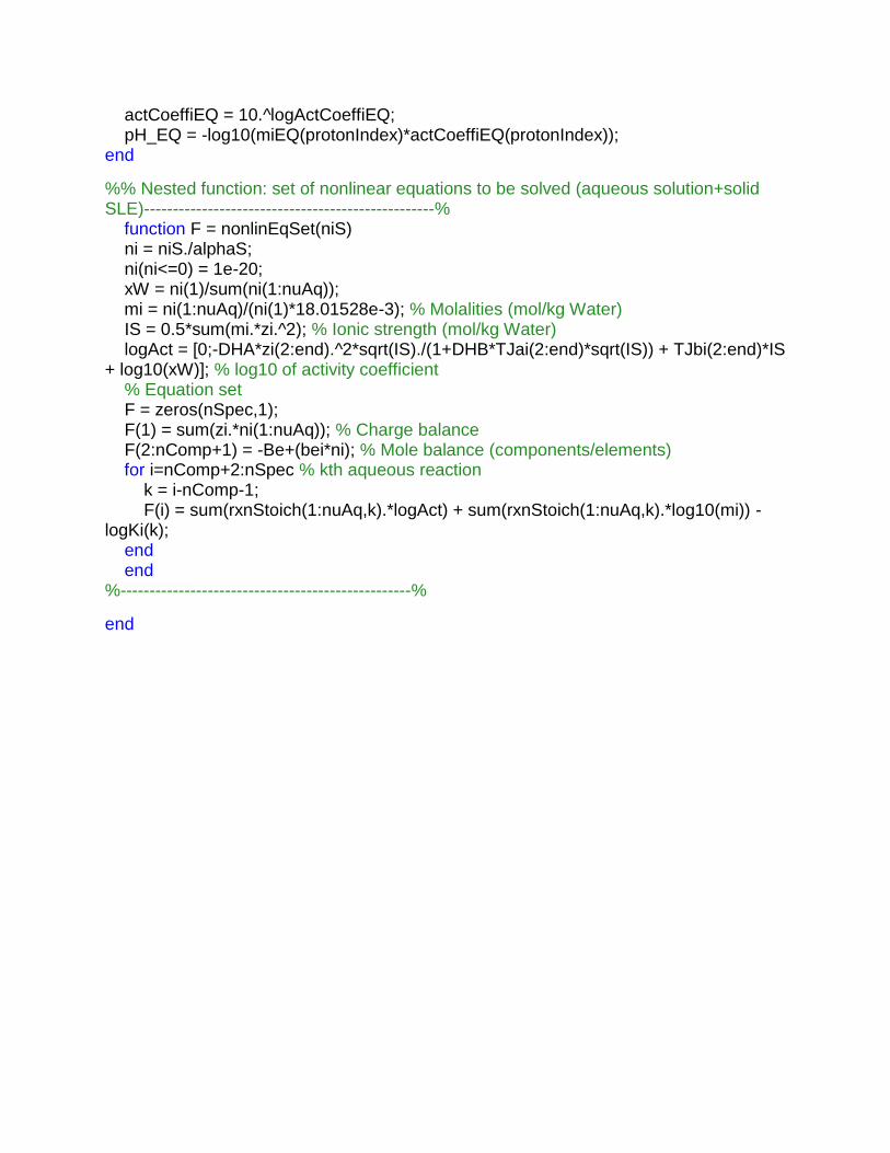
actCoeffiEQ = 10.^logActCoeffiEQ; pH_EQ = -log10(miEQ(protonIndex)*actCoeffiEQ(protonIndex)); end
%% Nested function: set of nonlinear equations to be solved (aqueous solution+solid SLE)--------------------------------------------------%
function F = nonlinEqSet(niS)
ni = niS./alphaS; ni(ni<=0) = 1e-20; xW = ni(1)/sum(ni(1:nuAq)); mi = ni(1:nuAq)/(ni(1)*18.01528e-3); % Molalities (mol/kg Water)
IS = 0.5*sum(mi.*zi.^2); % Ionic strength (mol/kg Water)
logAct = [0;-DHA*zi(2:end).^2*sqrt(IS)./(1+DHB*TJai(2:end)*sqrt(IS)) + TJbi(2:end)*IS + log10(xW)]; % log10 of activity coefficient % Equation set F = zeros(nSpec,1); F(1) = sum(zi.*ni(1:nuAq)); % Charge balance
F(2:nComp+1) = -Be+(bei*ni); % Mole balance (components/elements)
for i=nComp+2:nSpec % kth aqueous reaction
k = i-nComp-1; F(i) = sum(rxnStoich(1:nuAq,k).*logAct) + sum(rxnStoich(1:nuAq,k).*log10(mi)) - logKi(k); end
end
%--------------------------------------------------%
end
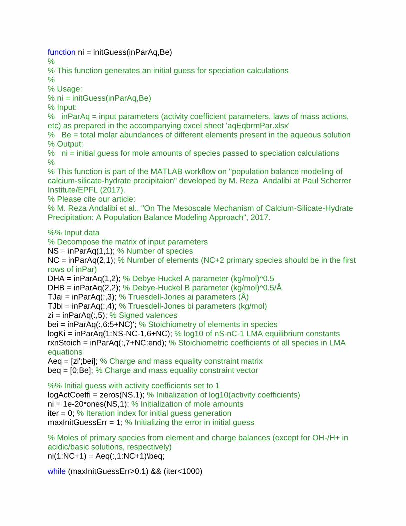
function ni = initGuess(inParAq,Be)
% % This function generates an initial guess for speciation calculations
% % Usage: % ni = initGuess(inParAq,Be)
% Input: % inParAq = input parameters (activity coefficient parameters, laws of mass actions, etc) as prepared in the accompanying excel sheet 'aqEqbrmPar.xlsx' % Be = total molar abundances of different elements present in the aqueous solution
% Output: % ni = initial guess for mole amounts of species passed to speciation calculations
% % This function is part of the MATLAB workflow on "population balance modeling of calcium-silicate-hydrate precipitaion" developed by M. Reza Andalibi at Paul Scherrer Institute/EPFL (2017). % Please cite our article: % M. Reza Andalibi et al., "On The Mesoscale Mechanism of Calcium-Silicate-Hydrate Precipitation: A Population Balance Modeling Approach", 2017. %% Input data
% Decompose the matrix of input parameters
NS = inParAq(1,1); % Number of species
NC = inParAq(2,1); % Number of elements (NC+2 primary species should be in the first rows of inPar)
DHA = inParAq(1,2); % Debye-Huckel A parameter (kg/mol)^0.5
DHB = inParAq(2,2); % Debye-Huckel B parameter (kg/mol)^0.5/Å
TJai = inParAq(:,3); % Truesdell-Jones ai parameters (Å)
TJbi = inParAq(:,4); % Truesdell-Jones bi parameters (kg/mol)
zi = inParAq(:,5); % Signed valences
bei = inParAq(:,6:5+NC)'; % Stoichiometry of elements in species
logKi = inParAq(1:NS-NC-1,6+NC); % log10 of nS-nC-1 LMA equilibrium constants
rxnStoich = inParAq(:,7+NC:end); % Stoichiometric coefficients of all species in LMA equations Aeq = [zi';bei]; % Charge and mass equality constraint matrix
beq = [0;Be]; % Charge and mass equality constraint vector
%% Initial guess with activity coefficients set to 1
logActCoeffi = zeros(NS,1); % Initialization of log10(activity coefficients)
ni = 1e-20*ones(NS,1); % Initialization of mole amounts
iter = 0; % Iteration index for initial guess generation
maxInitGuessErr = 1; % Initializing the error in initial guess
% Moles of primary species from element and charge balances (except for OH-/H+ in acidic/basic solutions, respectively)
ni(1:NC+1) = Aeq(:,1:NC+1)\beq; while (maxInitGuessErr>0.1) && (iter<1000)
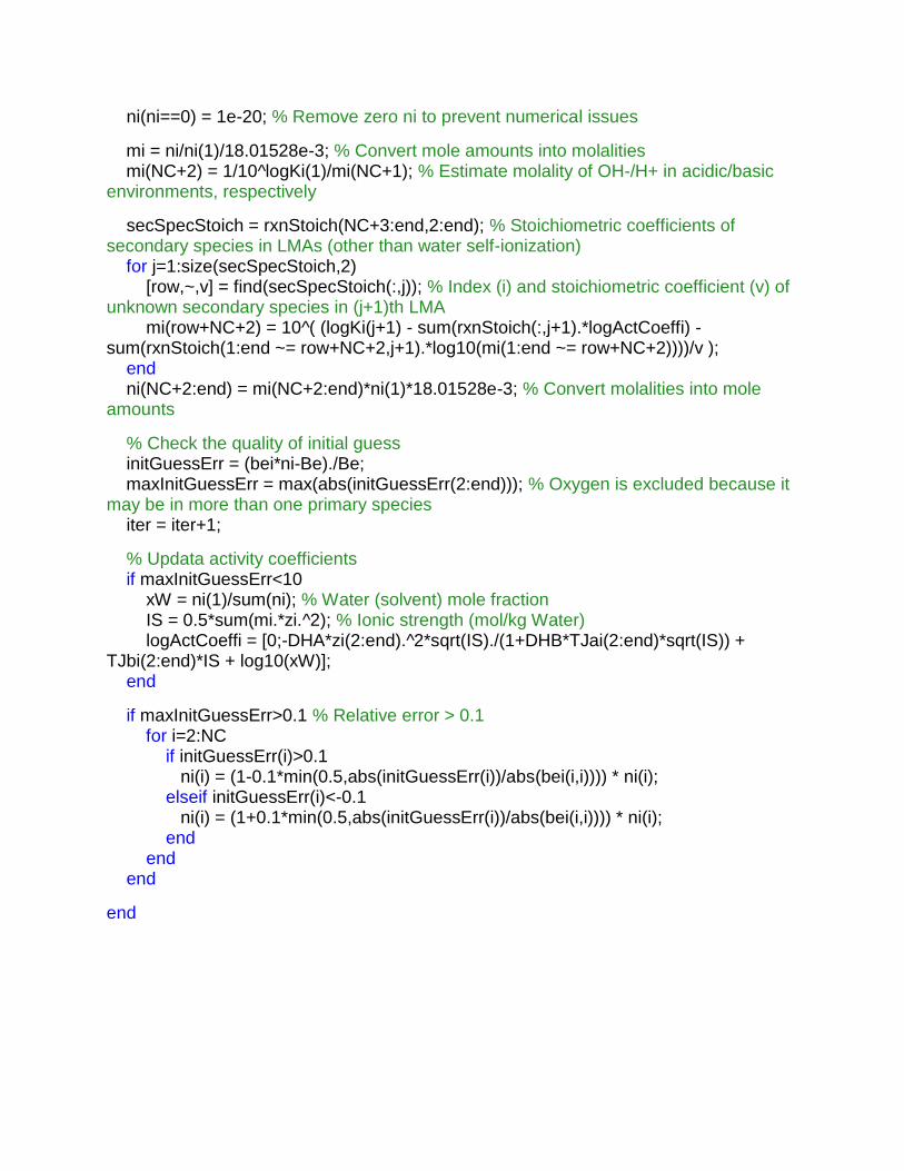
ni(ni==0) = 1e-20; % Remove zero ni to prevent numerical issues
mi = ni/ni(1)/18.01528e-3; % Convert mole amounts into molalities
mi(NC+2) = 1/10^logKi(1)/mi(NC+1); % Estimate molality of OH-/H+ in acidic/basic environments, respectively
secSpecStoich = rxnStoich(NC+3:end,2:end); % Stoichiometric coefficients of secondary species in LMAs (other than water self-ionization)
for j=1:size(secSpecStoich,2)
[row,~,v] = find(secSpecStoich(:,j)); % Index (i) and stoichiometric coefficient (v) of unknown secondary species in (j+1)th LMA
mi(row+NC+2) = 10^( (logKi(j+1) - sum(rxnStoich(:,j+1).*logActCoeffi) - sum(rxnStoich(1:end ~= row+NC+2,j+1).*log10(mi(1:end ~= row+NC+2))))/v );
end
ni(NC+2:end) = mi(NC+2:end)*ni(1)*18.01528e-3; % Convert molalities into mole amounts
% Check the quality of initial guess
initGuessErr = (bei*ni-Be)./Be; maxInitGuessErr = max(abs(initGuessErr(2:end))); % Oxygen is excluded because it may be in more than one primary species
iter = iter+1; % Updata activity coefficients
if maxInitGuessErr<10
xW = ni(1)/sum(ni); % Water (solvent) mole fraction
IS = 0.5*sum(mi.*zi.^2); % Ionic strength (mol/kg Water)
logActCoeffi = [0;-DHA*zi(2:end).^2*sqrt(IS)./(1+DHB*TJai(2:end)*sqrt(IS)) + TJbi(2:end)*IS + log10(xW)]; end
if maxInitGuessErr>0.1 % Relative error > 0.1
for i=2:NC
if initGuessErr(i)>0.1
ni(i) = (1-0.1*min(0.5,abs(initGuessErr(i))/abs(bei(i,i)))) * ni(i); elseif initGuessErr(i)<-0.1
ni(i) = (1+0.1*min(0.5,abs(initGuessErr(i))/abs(bei(i,i)))) * ni(i);
end
end
end
end

% This script calculates aqEQBRM data for C-S-H precipitation system and is part of the MATLAB workflow on
% "population balance modeling of calcium-silicate-hydrate precipitaion" developed by M. Reza Andalibi at Paul Scherrer Institute/EPFL (2017). % Please cite our article: % M. Reza Andalibi et al., "On The Mesoscale Mechanism of Calcium-Silicate-Hydrate Precipitation: A Population Balance Modeling Approach", 2017. clear; clc; inParAq = dlmread('inParAq.txt'); Be = dlmread('Be_2.0mL.min-1.txt'); % Be = dlmread('Be_0.5mL.min-1.txt'); eqNo = size(Be,1); niEQ = zeros(eqNo,15); miEQ = zeros(eqNo,15); actCoeffiEQ = zeros(eqNo,15); pH_EQ = zeros(eqNo,1); IS_EQ = zeros(eqNo,1); exitflag = zeros(eqNo,1); % parfor j=1:eqNo % If initial guesses are not available parallelization can expedite the computation
% [niEQ(j,:),miEQ(j,:),actCoeffiEQ(j,:),pH_EQ(j,1),IS_EQ(j,1),exitflag(j,1)] = aqEQBRM(inPar,Be(j,:)'); % end
j=1; [niEQ(j,:),miEQ(j,:),actCoeffiEQ(j,:),pH_EQ(j,1),IS_EQ(j,1),exitflag(j,1)] = aqEQBRM(inParAq,Be(j,:)'); for j=2:eqNo
[niEQ(j,:),miEQ(j,:),actCoeffiEQ(j,:),pH_EQ(j,1),IS_EQ(j,1),exitflag(j,1)] = aqEQBRM(inParAq,Be(j,:)',niEQ(j-1,:)'); end
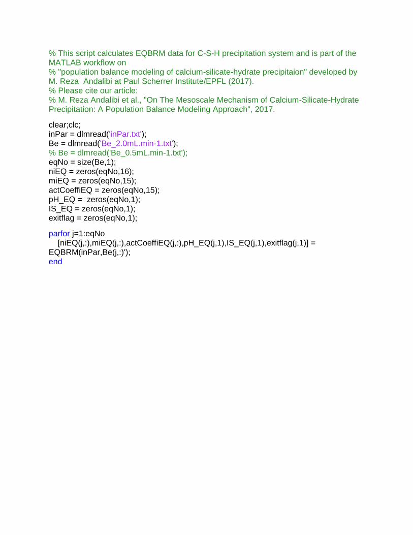
% This script calculates EQBRM data for C-S-H precipitation system and is part of the MATLAB workflow on
% "population balance modeling of calcium-silicate-hydrate precipitaion" developed by M. Reza Andalibi at Paul Scherrer Institute/EPFL (2017). % Please cite our article: % M. Reza Andalibi et al., "On The Mesoscale Mechanism of Calcium-Silicate-Hydrate Precipitation: A Population Balance Modeling Approach", 2017. clear;clc; inPar = dlmread('inPar.txt'); Be = dlmread('Be_2.0mL.min-1.txt'); % Be = dlmread('Be_0.5mL.min-1.txt'); eqNo = size(Be,1); niEQ = zeros(eqNo,16); miEQ = zeros(eqNo,15); actCoeffiEQ = zeros(eqNo,15); pH_EQ = zeros(eqNo,1); IS_EQ = zeros(eqNo,1); exitflag = zeros(eqNo,1); parfor j=1:eqNo
[niEQ(j,:),miEQ(j,:),actCoeffiEQ(j,:),pH_EQ(j,1),IS_EQ(j,1),exitflag(j,1)] = EQBRM(inPar,Be(j,:)'); end
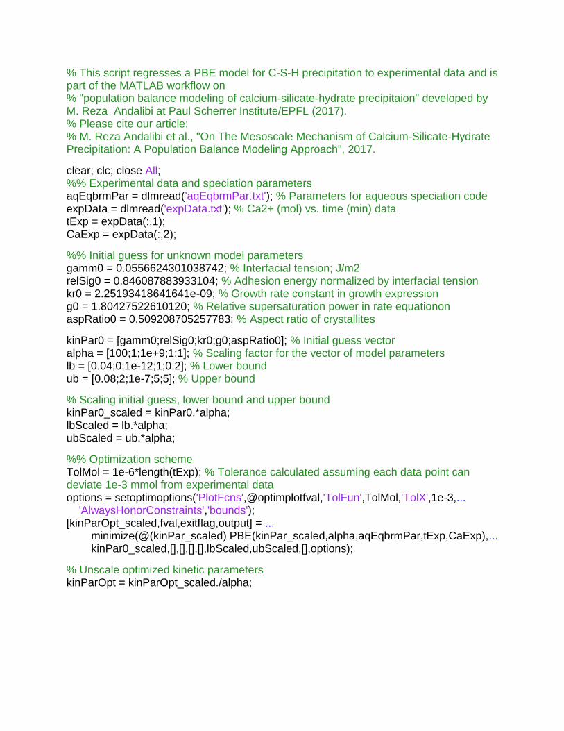
% This script regresses a PBE model for C-S-H precipitation to experimental data and is part of the MATLAB workflow on
% "population balance modeling of calcium-silicate-hydrate precipitaion" developed by M. Reza Andalibi at Paul Scherrer Institute/EPFL (2017). % Please cite our article: % M. Reza Andalibi et al., "On The Mesoscale Mechanism of Calcium-Silicate-Hydrate Precipitation: A Population Balance Modeling Approach", 2017. clear; clc; close All; %% Experimental data and speciation parameters
aqEqbrmPar = dlmread('aqEqbrmPar.txt'); % Parameters for aqueous speciation code
expData = dlmread('expData.txt'); % Ca2+ (mol) vs. time (min) data
tExp = expData(:,1); CaExp = expData(:,2); %% Initial guess for unknown model parameters
gamm0 = 0.0556624301038742; % Interfacial tension; J/m2
relSig0 = 0.846087883933104; % Adhesion energy normalized by interfacial tension
kr0 = 2.25193418641641e-09; % Growth rate constant in growth expression
g0 = 1.80427522610120; % Relative supersaturation power in rate equationon
aspRatio0 = 0.509208705257783; % Aspect ratio of crystallites
kinPar0 = [gamm0;relSig0;kr0;g0;aspRatio0]; % Initial guess vector
alpha = [100;1;1e+9;1;1]; % Scaling factor for the vector of model parameters
lb = [0.04;0;1e-12;1;0.2]; % Lower bound
ub = [0.08;2;1e-7;5;5]; % Upper bound
% Scaling initial guess, lower bound and upper bound
kinPar0_scaled = kinPar0.*alpha; lbScaled = lb.*alpha; ubScaled = ub.*alpha; %% Optimization scheme
TolMol = 1e-6*length(tExp); % Tolerance calculated assuming each data point can deviate 1e-3 mmol from experimental data
options = setoptimoptions('PlotFcns',@optimplotfval,'TolFun',TolMol,'TolX',1e-3,... 'AlwaysHonorConstraints','bounds'); [kinParOpt_scaled,fval,exitflag,output] = ... minimize(@(kinPar_scaled) PBE(kinPar_scaled,alpha,aqEqbrmPar,tExp,CaExp),... kinPar0_scaled,[],[],[],[],lbScaled,ubScaled,[],options); % Unscale optimized kinetic parameters
kinParOpt = kinParOpt_scaled./alpha;
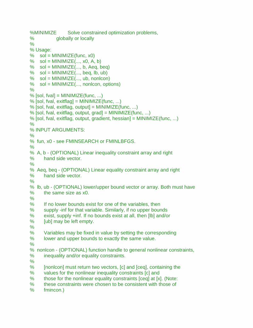
%MINIMIZE Solve constrained optimization problems, % globally or locally
%
% Usage: % sol = MINIMIZE(func, x0) % sol = MINIMIZE(..., x0, A, b) % sol = MINIMIZE(..., b, Aeq, beq) % sol = MINIMIZE(..., beq, lb, ub)
% sol = MINIMIZE(..., ub, nonlcon) % sol = MINIMIZE(..., nonlcon, options) %
% [sol, fval] = MINIMIZE(func, ...)
% [sol, fval, exitflag] = MINIMIZE(func, ...)
% [sol, fval, exitflag, output] = MINIMIZE(func, ...)
% [sol, fval, exitflag, output, grad] = MINIMIZE(func, ...)
% [sol, fval, exitflag, output, gradient, hessian] = MINIMIZE(func, ...)
%
% INPUT ARGUMENTS: %
% fun, x0 - see FMINSEARCH or FMINLBFGS. %
% A, b - (OPTIONAL) Linear inequality constraint array and right % hand side vector. %
% Aeq, beq - (OPTIONAL) Linear equality constraint array and right % hand side vector. %
% lb, ub - (OPTIONAL) lower/upper bound vector or array. Both must have % the same size as x0. %
% If no lower bounds exist for one of the variables, then
% supply -inf for that variable. Similarly, if no upper bounds % exist, supply +inf. If no bounds exist at all, then [lb] and/or % [ub] may be left empty. %
% Variables may be fixed in value by setting the corresponding
% lower and upper bounds to exactly the same value. %
% nonlcon - (OPTIONAL) function handle to general nonlinear constraints, % inequality and/or equality constraints. %
% [nonlcon] must return two vectors, [c] and [ceq], containing the
% values for the nonlinear inequality constraints [c] and
% those for the nonlinear equality constraints [ceq] at [x]. (Note: % these constraints were chosen to be consistent with those of % fmincon.)
%
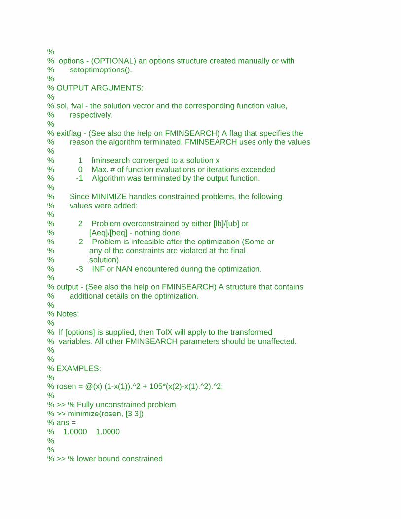
% options - (OPTIONAL) an options structure created manually or with
% setoptimoptions(). % % OUTPUT ARGUMENTS: %
% sol, fval - the solution vector and the corresponding function value,
% respectively. %
% exitflag - (See also the help on FMINSEARCH) A flag that specifies the % reason the algorithm terminated. FMINSEARCH uses only the values
%
% 1 fminsearch converged to a solution x
% 0 Max. # of function evaluations or iterations exceeded
% -1 Algorithm was terminated by the output function. %
% Since MINIMIZE handles constrained problems, the following % values were added: %
% 2 Problem overconstrained by either [lb]/[ub] or
% [Aeq]/[beq] - nothing done
% -2 Problem is infeasible after the optimization (Some or % any of the constraints are violated at the final % solution). % -3 INF or NAN encountered during the optimization. %
% output - (See also the help on FMINSEARCH) A structure that contains
% additional details on the optimization. %
% Notes: %
% If [options] is supplied, then TolX will apply to the transformed
% variables. All other FMINSEARCH parameters should be unaffected. %
%
% EXAMPLES: %
% rosen = @(x) (1-x(1)).^2 + 105*(x(2)-x(1).^2).^2; %
% >> % Fully unconstrained problem
% >> minimize(rosen, [3 3])
% ans =
% 1.0000 1.0000
%
%
% >> % lower bound constrained
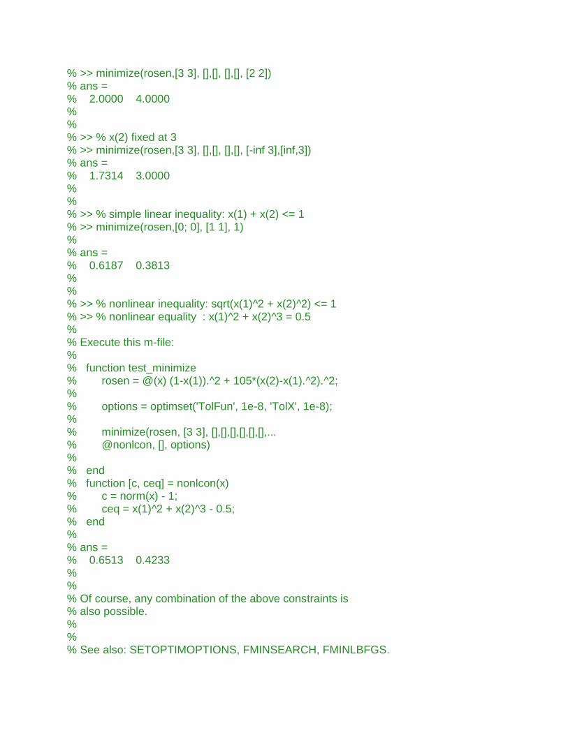
% >> minimize(rosen,[3 3], [],[], [],[], [2 2])
% ans =
% 2.0000 4.0000
%
%
% >> % x(2) fixed at 3
% >> minimize(rosen,[3 3], [],[], [],[], [-inf 3],[inf,3])
% ans =
% 1.7314 3.0000
%
%
% >> % simple linear inequality: x(1) + x(2) <= 1
% >> minimize(rosen,[0; 0], [1 1], 1)
% % ans =
% 0.6187 0.3813
% %
% >> % nonlinear inequality: sqrt(x(1)^2 + x(2)^2) <= 1
% >> % nonlinear equality : x(1)^2 + x(2)^3 = 0.5
%
% Execute this m-file: %
% function test_minimize
% rosen = @(x) (1-x(1)).^2 + 105*(x(2)-x(1).^2).^2; %
% options = optimset('TolFun', 1e-8, 'TolX', 1e-8); %
% minimize(rosen, [3 3], [],[],[],[],[],[],... % @nonlcon, [], options)
%
% end
% function [c, ceq] = nonlcon(x)
% c = norm(x) - 1; % ceq = x(1)^2 + x(2)^3 - 0.5; % end
%
% ans =
% 0.6513 0.4233
%
%
% Of course, any combination of the above constraints is
% also possible. %
%
% See also: SETOPTIMOPTIONS, FMINSEARCH, FMINLBFGS.
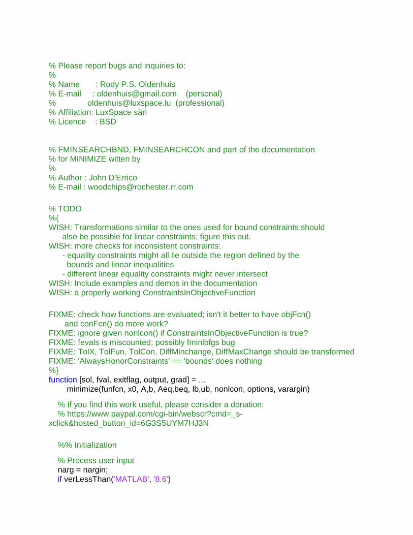
% Please report bugs and inquiries to: %
% Name : Rody P.S. Oldenhuis
% E-mail : [email protected] (personal)
% [email protected] (professional)
% Affiliation: LuxSpace sàrl % Licence : BSD
% FMINSEARCHBND, FMINSEARCHCON and part of the documentation % for MINIMIZE witten by
%
% Author : John D'Errico
% E-mail : [email protected]
% TODO
%{
WISH: Transformations similar to the ones used for bound constraints should
also be possible for linear constraints; figure this out. WISH: more checks for inconsistent constraints: - equality constraints might all lie outside the region defined by the bounds and linear inequalities
- different linear equality constraints might never intersect WISH: Include examples and demos in the documentation
WISH: a properly working ConstraintsInObjectiveFunction
FIXME: check how functions are evaluated; isn't it better to have objFcn()
and conFcn() do more work? FIXME: ignore given nonlcon() if ConstraintsInObjectiveFunction is true?
FIXME: fevals is miscounted; possibly fminlbfgs bug
FIXME: TolX, TolFun, TolCon, DiffMinchange, DiffMaxChange should be transformed
FIXME: 'AlwaysHonorConstraints' == 'bounds' does nothing
%}
function [sol, fval, exitflag, output, grad] = ... minimize(funfcn, x0, A,b, Aeq,beq, lb,ub, nonlcon, options, varargin)
% If you find this work useful, please consider a donation: % https://www.paypal.com/cgi-bin/webscr?cmd=_s-xclick&hosted_button_id=6G3S5UYM7HJ3N
%% Initialization
% Process user input narg = nargin; if verLessThan('MATLAB', '8.6')
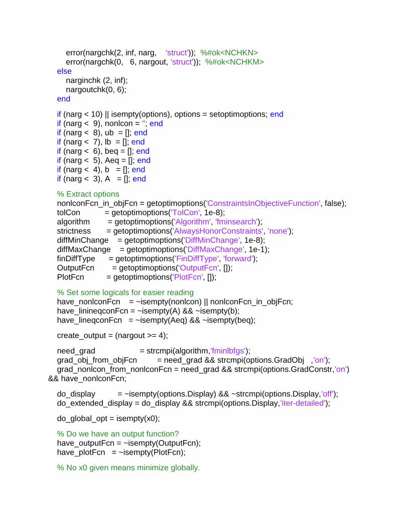
error(nargchk(2, inf, narg, 'struct')); %#ok<NCHKN>
error(nargchk(0, 6, nargout, 'struct')); %#ok<NCHKM>
else
narginchk (2, inf); nargoutchk(0, 6); end
if (narg < 10) || isempty(options), options = setoptimoptions; end
if (narg < 9), nonlcon = ''; end
if (narg < 8), ub = []; end
if (narg < 7), lb = []; end
if (narg < 6), beq = []; end
if (narg < 5), Aeq = []; end
if (narg < 4), b = []; end
if (narg < 3), A = []; end
% Extract options
nonlconFcn_in_objFcn = getoptimoptions('ConstraintsInObjectiveFunction', false); tolCon = getoptimoptions('TolCon', 1e-8); algorithm = getoptimoptions('Algorithm', 'fminsearch'); strictness = getoptimoptions('AlwaysHonorConstraints', 'none'); diffMinChange = getoptimoptions('DiffMinChange', 1e-8); diffMaxChange = getoptimoptions('DiffMaxChange', 1e-1); finDiffType = getoptimoptions('FinDiffType', 'forward'); OutputFcn = getoptimoptions('OutputFcn', []); PlotFcn = getoptimoptions('PlotFcn', []); % Set some logicals for easier reading
have_nonlconFcn = ~isempty(nonlcon) || nonlconFcn_in_objFcn;
have_linineqconFcn = ~isempty(A) && ~isempty(b); have_lineqconFcn = ~isempty(Aeq) && ~isempty(beq); create_output = (nargout >= 4); need_grad = strcmpi(algorithm,'fminlbfgs'); grad_obj_from_objFcn = need_grad && strcmpi(options.GradObj ,'on'); grad_nonlcon_from_nonlconFcn = need_grad && strcmpi(options.GradConstr,'on') && have_nonlconFcn; do_display = ~isempty(options.Display) && ~strcmpi(options.Display,'off'); do_extended_display = do_display && strcmpi(options.Display,'iter-detailed'); do_global_opt = isempty(x0); % Do we have an output function? have_outputFcn = ~isempty(OutputFcn); have_plotFcn = ~isempty(PlotFcn); % No x0 given means minimize globally.
if do_global_opt [sol, fval, exitflag, output] = minimize_globally();
return; end
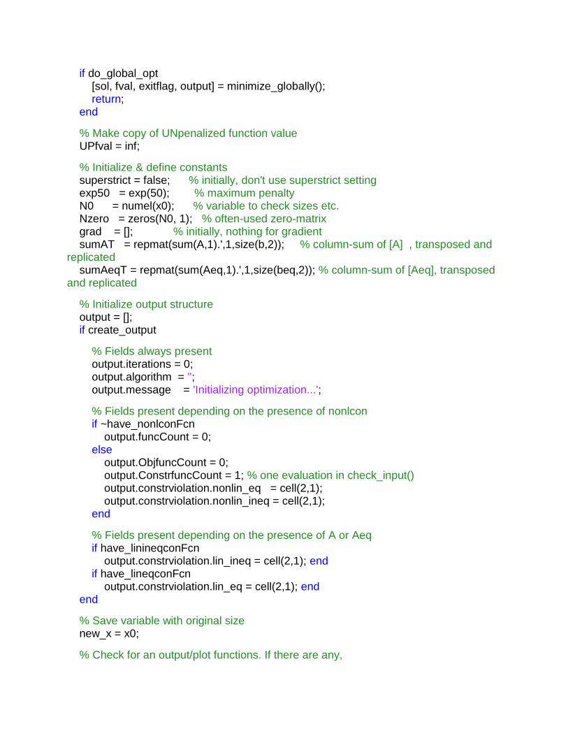
% Make copy of UNpenalized function value
UPfval = inf; % Initialize & define constants superstrict = false; % initially, don't use superstrict setting exp50 = exp(50); % maximum penalty
N0 = numel(x0); % variable to check sizes etc. Nzero = zeros(N0, 1); % often-used zero-matrix grad = []; % initially, nothing for gradient sumAT = repmat(sum(A,1).',1,size(b,2)); % column-sum of [A] , transposed and replicated
sumAeqT = repmat(sum(Aeq,1).',1,size(beq,2)); % column-sum of [Aeq], transposed and replicated
% Initialize output structure
output = []; if create_output % Fields always present output.iterations = 0; output.algorithm = ''; output.message = 'Initializing optimization...'; % Fields present depending on the presence of nonlcon
if ~have_nonlconFcn
output.funcCount = 0; else
output.ObjfuncCount = 0; output.ConstrfuncCount = 1; % one evaluation in check_input()
output.constrviolation.nonlin_eq = cell(2,1); output.constrviolation.nonlin_ineq = cell(2,1); end
% Fields present depending on the presence of A or Aeq
if have_linineqconFcn
output.constrviolation.lin_ineq = cell(2,1); end
if have_lineqconFcn
output.constrviolation.lin_eq = cell(2,1); end
end
% Save variable with original size new_x = x0; % Check for an output/plot functions. If there are any,
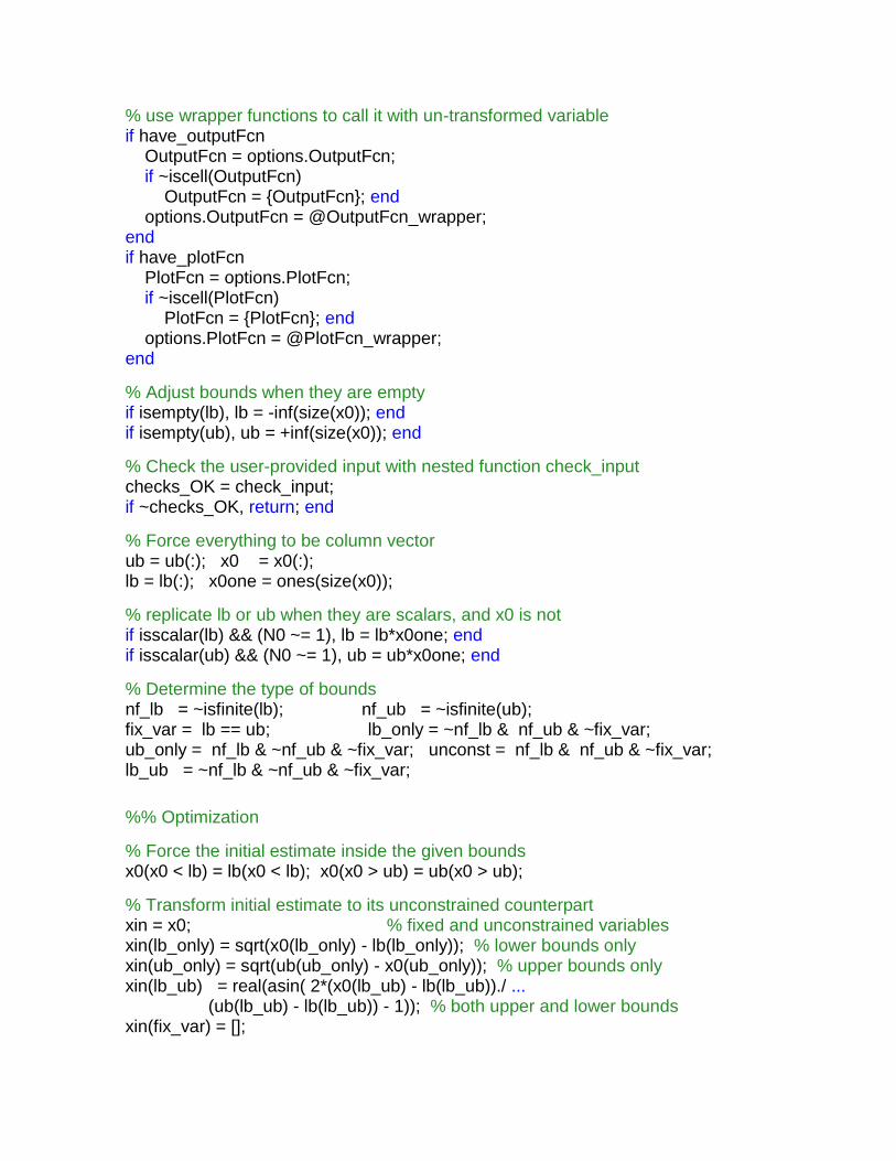
% use wrapper functions to call it with un-transformed variable
if have_outputFcn
OutputFcn = options.OutputFcn; if ~iscell(OutputFcn)
OutputFcn = {OutputFcn}; end
options.OutputFcn = @OutputFcn_wrapper; end if have_plotFcn
PlotFcn = options.PlotFcn; if ~iscell(PlotFcn)
PlotFcn = {PlotFcn}; end
options.PlotFcn = @PlotFcn_wrapper; end % Adjust bounds when they are empty
if isempty(lb), lb = -inf(size(x0)); end
if isempty(ub), ub = +inf(size(x0)); end
% Check the user-provided input with nested function check_input checks_OK = check_input; if ~checks_OK, return; end % Force everything to be column vector
ub = ub(:); x0 = x0(:); lb = lb(:); x0one = ones(size(x0)); % replicate lb or ub when they are scalars, and x0 is not if isscalar(lb) && (N0 ~= 1), lb = lb*x0one; end
if isscalar(ub) && (N0 ~= 1), ub = ub*x0one; end % Determine the type of bounds
nf_lb = ~isfinite(lb); nf_ub = ~isfinite(ub); fix_var = lb == ub; lb_only = ~nf_lb & nf_ub & ~fix_var;
ub_only = nf_lb & ~nf_ub & ~fix_var; unconst = nf_lb & nf_ub & ~fix_var;
lb_ub = ~nf_lb & ~nf_ub & ~fix_var; %% Optimization % Force the initial estimate inside the given bounds
x0(x0 < lb) = lb(x0 < lb); x0(x0 > ub) = ub(x0 > ub); % Transform initial estimate to its unconstrained counterpart xin = x0; % fixed and unconstrained variables xin(lb_only) = sqrt(x0(lb_only) - lb(lb_only)); % lower bounds only xin(ub_only) = sqrt(ub(ub_only) - x0(ub_only)); % upper bounds only
xin(lb_ub) = real(asin( 2*(x0(lb_ub) - lb(lb_ub))./ ... (ub(lb_ub) - lb(lb_ub)) - 1)); % both upper and lower bounds
xin(fix_var) = [];
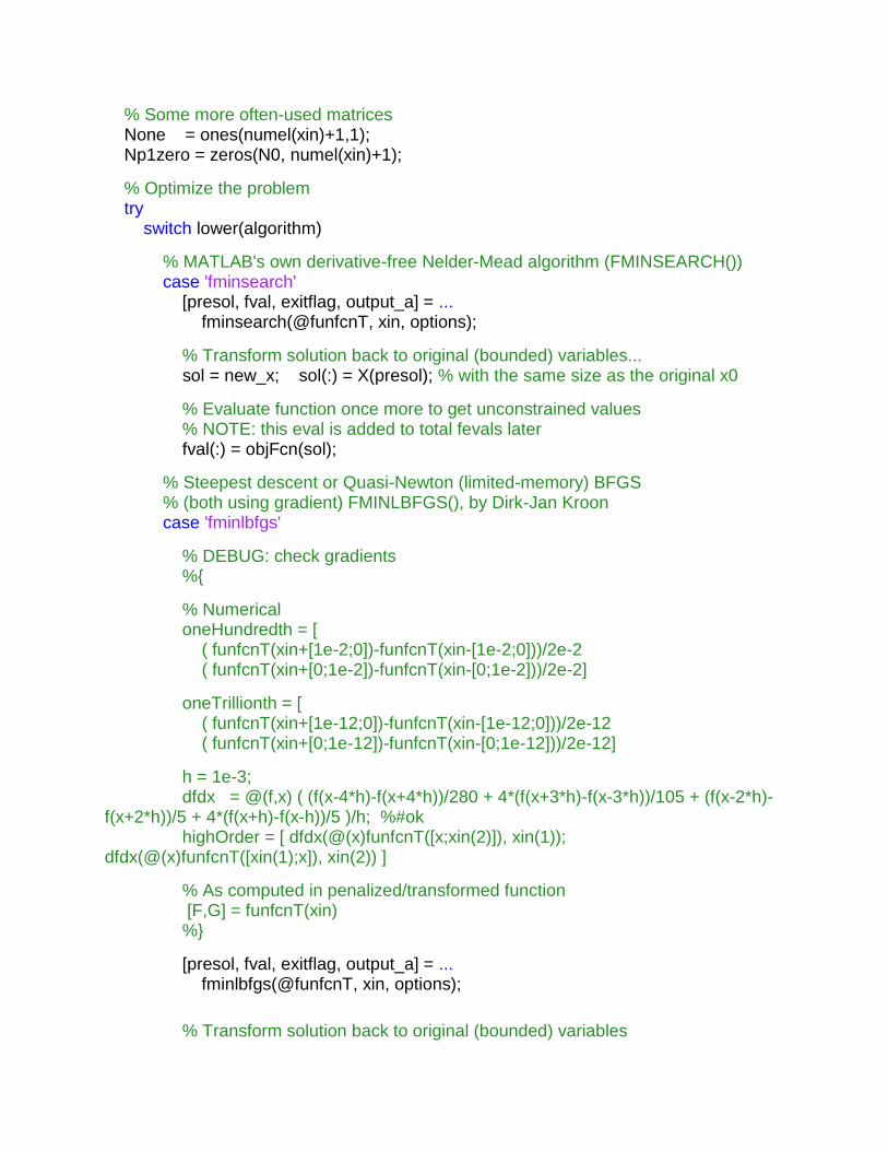
% Some more often-used matrices
None = ones(numel(xin)+1,1); Np1zero = zeros(N0, numel(xin)+1); % Optimize the problem
try
switch lower(algorithm)
% MATLAB's own derivative-free Nelder-Mead algorithm (FMINSEARCH())
case 'fminsearch' [presol, fval, exitflag, output_a] = ... fminsearch(@funfcnT, xin, options); % Transform solution back to original (bounded) variables...
sol = new_x; sol(:) = X(presol); % with the same size as the original x0
% Evaluate function once more to get unconstrained values
% NOTE: this eval is added to total fevals later
fval(:) = objFcn(sol); % Steepest descent or Quasi-Newton (limited-memory) BFGS % (both using gradient) FMINLBFGS(), by Dirk-Jan Kroon case 'fminlbfgs' % DEBUG: check gradients
%{
% Numerical oneHundredth = [ ( funfcnT(xin+[1e-2;0])-funfcnT(xin-[1e-2;0]))/2e-2
( funfcnT(xin+[0;1e-2])-funfcnT(xin-[0;1e-2]))/2e-2] oneTrillionth = [ ( funfcnT(xin+[1e-12;0])-funfcnT(xin-[1e-12;0]))/2e-12
( funfcnT(xin+[0;1e-12])-funfcnT(xin-[0;1e-12]))/2e-12] h = 1e-3; dfdx = @(f,x) ( (f(x-4*h)-f(x+4*h))/280 + 4*(f(x+3*h)-f(x-3*h))/105 + (f(x-2*h)-f(x+2*h))/5 + 4*(f(x+h)-f(x-h))/5 )/h; %#ok
highOrder = [ dfdx(@(x)funfcnT([x;xin(2)]), xin(1)); dfdx(@(x)funfcnT([xin(1);x]), xin(2)) ] % As computed in penalized/transformed function
[F,G] = funfcnT(xin)
%}
[presol, fval, exitflag, output_a] = ... fminlbfgs(@funfcnT, xin, options); % Transform solution back to original (bounded) variables
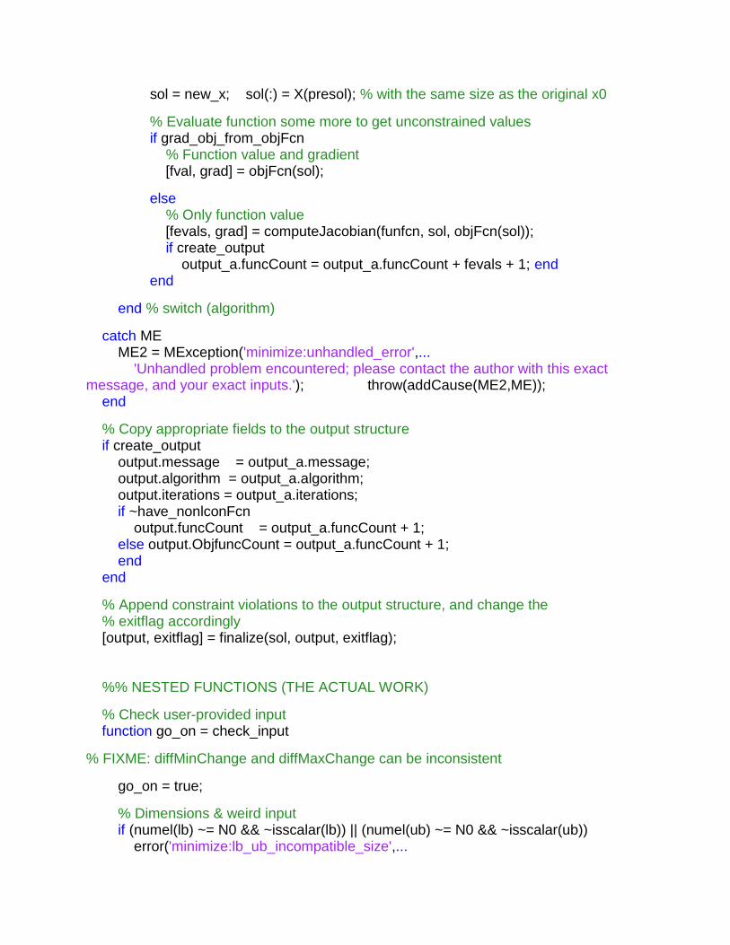
sol = new_x; sol(:) = X(presol); % with the same size as the original x0 % Evaluate function some more to get unconstrained values
if grad_obj_from_objFcn
% Function value and gradient [fval, grad] = objFcn(sol); else
% Only function value
[fevals, grad] = computeJacobian(funfcn, sol, objFcn(sol)); if create_output output_a.funcCount = output_a.funcCount + fevals + 1; end
end
end % switch (algorithm)
catch ME ME2 = MException('minimize:unhandled_error',... 'Unhandled problem encountered; please contact the author with this exact message, and your exact inputs.'); throw(addCause(ME2,ME)); end
% Copy appropriate fields to the output structure
if create_output output.message = output_a.message; output.algorithm = output_a.algorithm; output.iterations = output_a.iterations; if ~have_nonlconFcn
output.funcCount = output_a.funcCount + 1; else output.ObjfuncCount = output_a.funcCount + 1; end
end
% Append constraint violations to the output structure, and change the
% exitflag accordingly
[output, exitflag] = finalize(sol, output, exitflag); %% NESTED FUNCTIONS (THE ACTUAL WORK)
% Check user-provided input function go_on = check_input % FIXME: diffMinChange and diffMaxChange can be inconsistent go_on = true; % Dimensions & weird input if (numel(lb) ~= N0 && ~isscalar(lb)) || (numel(ub) ~= N0 && ~isscalar(ub))
error('minimize:lb_ub_incompatible_size',...
'Size of either [lb] or [ub] incompatible with size of [x0].')
end
if ~isempty(A) && isempty(b)
warning('minimize:Aeq_but_not_beq', ... ['I received the matrix [A], but you omitted the corresponding vector [b].',... '\nI''ll assume a zero-vector for [b]...'])
b = zeros(size(A,1), size(x0,2)); end
if ~isempty(Aeq) && isempty(beq)
warning('minimize:Aeq_but_not_beq', ... ['I received the matrix [Aeq], but you omitted the corresponding vector [beq].',... '\nI''ll assume a zero-vector for [beq]...'])
beq = zeros(size(Aeq,1), size(x0,2)); end
if isempty(Aeq) && ~isempty(beq)
warning('minimize:beq_but_not_Aeq', ... ['I received the vector [beq], but you omitted the corresponding matrix [Aeq].',... '\nI''ll ignore the given [beq]...'])
beq = []; end
if isempty(A) && ~isempty(b)
warning('minimize:b_but_not_A', ... ['I received the vector [b], but you omitted the corresponding matrix [A].',... '\nI''ll ignore the given [b]...'])
b = []; end
if have_linineqconFcn && size(b,1)~=size(A,1)
error('minimize:b_incompatible_with_A',... 'The size of [b] is incompatible with that of [A].')
end
if have_lineqconFcn && size(beq,1)~=size(Aeq,1)
error('minimize:b_incompatible_with_A',... 'The size of [beq] is incompatible with that of [Aeq].')
end
if ~isvector(x0) && ~isempty(A) && (size(A,2) ~= size(x0,1))
error('minimize:A_incompatible_size',... 'Linear constraint matrix [A] has incompatible size for given [x0].')
end
if ~isvector(x0) && ~isempty(Aeq) && (size(Aeq,2) ~= size(x0,1))
error('minimize:Aeq_incompatible_size',... 'Linear constraint matrix [Aeq] has incompatible size for given [x0].')
end
if ~isempty(b) && size(b,2)~=size(x0,2)
error('minimize:x0_vector_but_not_b',...
'Given linear constraint vector [b] has incompatible size with given [x0].')
end
if ~isempty(beq) && size(beq,2)~=size(x0,2)
error('minimize:x0_vector_but_not_beq',... 'Given linear constraint vector [beq] has incompatible size with given [x0].')
end % Functions are not function handles if ~isa(funfcn, 'function_handle')
error('minimize:func_not_a_function',... 'Objective function must be given as a function handle.')
end
if ~isempty(nonlcon) && ~ischar(nonlcon) && ~isa(nonlcon, 'function_handle')
error('minimize:nonlcon_not_a_function', ... 'non-linear constraint function must be a function handle (advised) or string (discouraged).')
end
% Check if FMINLBFGS can be executed
%FIXME: not required when you paste it as nested function below
% if ~isempty(algorithm) && strcmpi(algorithm,'fminlbfgs') && isempty(which('fminlbfgs'))
% error('minimize:fminlbfgs_not_present',... % 'The function FMINLBFGS is not present in the current MATLAB path.');
% end
% evaluate the non-linear constraint function on % the initial value, to perform initial checks
% FIXME: fevals not counted
grad_c = []; grad_ceq = []; [c, ceq] = conFcn(x0); % Check sizes of derivatives
if ~isempty(grad_c) && (size(grad_c,2) ~= numel(x0)) && (size(grad_c,1) ~= numel(x0))
error('minimize:grad_c_incorrect_size',... ['The matrix of gradients of the non-linear in-equality constraints\n',... 'must have one of its dimensions equal to the number of elements in [x].']); end
if ~isempty(grad_ceq) && (size(grad_ceq,2) ~= numel(x0)) && (size(grad_ceq,1) ~= numel(x0))
error('minimize:grad_ceq_incorrect_size',... ['The matrix of gradients of the non-linear equality constraints\n',... 'must have one of its dimension equal to the number of elements in [x].']); end
% Test the feasibility of the initial solution (when strict or
% superstrict behavior has been enabled) if strcmpi(strictness, 'Bounds') || strcmpi(strictness, 'All')
superstrict = strcmpi(strictness, 'All'); if ~isempty(A) && any(any(A*x0 > b))
error('minimize:x0_doesnt_satisfy_linear_ineq', ... ['Initial estimate does not satisfy linear inequality.', ... '\nPlease provide an initial estimate inside the feasible region.']); end
if ~isempty(Aeq) && any(any(Aeq*x0 ~= beq))
error('minimize:x0_doesnt_satisfy_linear_eq', ... ['Initial estimate does not satisfy linear equality.', ... '\nPlease provide an initial estimate inside the feasible region.']); end
if have_nonlconFcn
% check [c] if ~isempty(c) && any(c(:) > ~superstrict*tolCon) error('minimize:x0_doesnt_satisfy_nonlinear_ineq', ... ['Initial estimate does not satisfy nonlinear inequality.', ... '\nPlease provide an initial estimate inside the feasible region.']); end
% check [ceq] if ~isempty(ceq) && any(abs(ceq(:)) >= ~superstrict*tolCon) error('minimize:x0_doesnt_satisfy_nonlinear_eq', ... ['Initial estimate does not satisfy nonlinear equality.', ... '\nPlease provide an initial estimate inside the feasible region.']); end
end
end % Detect and handle degenerate problems
% FIXME: with linear constraints it should be easy to determine if the
% constraints make feasible solutions impossible... % Impossible constraints
inds = all(A==0,2); if any(inds) && any(any(b(inds,:)>0))
error('minimize:impossible_linear_inequality',... 'Impossible linear inequality specified.'); end
inds = all(Aeq==0,2); if any(inds) && any(any(beq(inds,:)~=0))
error('minimize:impossible_linear_equality',... 'Impossible linear equality specified.'); end
% Degenerate constraints
if size(Aeq,1) > N0 && rank(Aeq) == N0
warning('minimize:linear_equality_overconstrains',... 'Linear equalities overconstrain problem; constrain violation is likely.'); end
if size(Aeq,2) >= N0 && rank(Aeq) >= N0
% warning('minimize:linear_equality_overconstrains',... % 'Linear equalities define solution - nothing to do.'); sol = Aeq\beq; fval = objFcn(sol); new_x = sol; exitflag = 2; if create_output output.iterations = 0; output.message = 'Linear equalities define solution; nothing to do.'; if ~have_nonlconFcn
output.funcCount = 1; else output.ObjfuncCount = 1; end
end
do_display_P = do_display; do_display = false; [output, exitflag] = finalize(sol, output, exitflag); if create_output && exitflag ~= -2
output.message = sprintf(... '%s\nFortunately, the solution is feasible using OPTIONS.TolCon of %1.6f.',... output.message, tolCon); end
if do_display_P
fprintf(1, output.message); end go_on = false; return; end
% If all variables are fixed, simply return
if sum(lb(:)==ub(:)) == N0
% warning('minimize:bounds_overconstrain',... % 'Lower and upper bound are equal - nothing to do.'); sol = reshape(lb,size(x0)); fval = objFcn(sol);
new_x = sol; exitflag = 2; if create_output output.iterations = 0; output.message = 'Lower and upper bound were set equal - nothing to do. '; if ~have_nonlconFcn
output.funcCount = 1; else output.ObjfuncCount = 1; end
end
do_display_P = do_display; do_display = false; [output, exitflag] = finalize(sol, output, exitflag); if create_output && exitflag ~= -2
output.message = sprintf(... '%s\nFortunately, the solution is feasible using OPTIONS.TolCon of %1.6f.',... output.message, tolCon); end if do_display_P
fprintf(1, output.message); end go_on = false; return; end
end % check_input % Evaluate objective function
function varargout = objFcn(x)
[varargout{1:nargout}] = feval(funfcn,... reshape(x,size(new_x)),... varargin{:}); end
% Evaluate non-linear constraint function
function [c,ceq, grad_c,grad_ceq] = conFcn(x)
c = []; ceq = []; grad_c = []; grad_ceq = []; x = reshape(x,size(new_x));
if have_nonlconFcn
if nonlconFcn_in_objFcn
if grad_nonlcon_from_nonlconFcn
if grad_obj_from_objFcn
[~,~, c, ceq, grad_c, grad_ceq] = objFcn(x); else
[~, c, ceq, grad_c, grad_ceq] = objFcn(x); end
else
if grad_obj_from_objFcn
[~,~, c, ceq] = objFcn(x); else
[~, c, ceq] = objFcn(x); end
end
else
if grad_nonlcon_from_nonlconFcn
[c, ceq, grad_c, grad_ceq] = feval(nonlcon, x, varargin{:}); else
[c, ceq] = feval(nonlcon, x, varargin{:}); end
end
end end
% Create transformed variable X to conform to upper and lower bounds
function Z = X(x)
% Initialize if (size(x,2) == 1)
Z = Nzero; rep = 1; else
Z = Np1zero; rep = None; end % First insert fixed values... y = x0one(:, rep); y( fix_var,:) = lb(fix_var,rep); y(~fix_var,:) = x; x = y; % ...and transform. Z(lb_only, :) = lb(lb_only, rep) + x(lb_only, :).^2;
Z(ub_only, :) = ub(ub_only, rep) - x(ub_only, :).^2; Z(fix_var, :) = lb(fix_var, rep); Z(unconst, :) = x(unconst, :); Z(lb_ub, :) = lb(lb_ub, rep) + (ub(lb_ub, rep)-lb(lb_ub, rep)) .* ...
(sin(x(lb_ub, :)) + 1)/2; end % X
% Derivatives of transformed X function grad_Z = gradX(x, grad_x)
% ...and compute gradient grad_Z = grad_x(~fix_var);
grad_Z(lb_only(~fix_var), :) = +2*grad_x(lb_only(~fix_var), :).*x(lb_only(~fix_var), :); grad_Z(ub_only(~fix_var), :) = -2*grad_x(ub_only(~fix_var), :).*x(ub_only(~fix_var), :); grad_Z(unconst(~fix_var), :) = grad_x(unconst(~fix_var), :);
grad_Z(lb_ub(~fix_var), :) = grad_x(lb_ub(~fix_var),:).*(ub(lb_ub(~fix_var),:)-lb(lb_ub(~fix_var),:)).*cos(x(lb_ub(~fix_var),:))/2; end % grad_Z
% Create penalized function. Penalize with linear penalty function if % violation is severe, otherwise, use exponential penalty. If the
% 'strict' option has been set, check the constraints, and return INF
% if any of them are violated. function [P_fval, grad_val] = funfcnP(x)
% FIXME: FMINSEARCH() or FMINLBFGS() see this as ONE function
% evaluation. However, multiple evaluations of both objective and nonlinear
% constraint functions may take place
% Initialize function value
if (size(x,2) == 1), P_fval = 0; else P_fval = None.'-1; end
% Initialize x_new array
x_new = new_x; % Initialize gradient when needed
if grad_obj_from_objFcn
grad_val = zeros(size(x)); end
% Evaluate every column in x
for ii = 1:size(x,2)
% Reshape x, so it has the same size as the given x0
x_new(:) = x(:,ii); % Initialize
obj_gradient = 0; c = []; ceq = []; grad_c = []; grad_ceq = []; % Evaluate the objective function, taking care that also

% a gradient and/or contstraint function may be supplied
if grad_obj_from_objFcn if ~nonlconFcn_in_objFcn
[obj_fval, obj_gradient] = objFcn(x_new); else
if grad_nonlcon_from_nonlconFcn
arg_out = cell(1, nonlconFcn_in_objFcn+1); else arg_out = cell(1, nonlconFcn_in_objFcn+3); end
[arg_out{:}] = objFcn(x_new); obj_fval = arg_out{1}; obj_gradient = arg_out{2}; c = arg_out{nonlconFcn_in_objFcn+0}; ceq = arg_out{nonlconFcn_in_objFcn+1}; if grad_nonlcon_from_nonlconFcn
grad_c = arg_out{nonlconFcn_in_objFcn+2}; grad_ceq = arg_out{nonlconFcn_in_objFcn+3}; else
grad_c = ''; % use strings to distinguish them later on
grad_ceq = ''; end
end
objFcn_fevals = 1; else
% FIXME: grad_nonlcon_from_nonlconFcn?
if ~nonlconFcn_in_objFcn
obj_fval = objFcn(x_new); else arg_out = cell(1, nonlconFcn_in_objFcn+1); [arg_out{:}] = objFcn(x_new); obj_fval = arg_out{1}; c = arg_out{nonlconFcn_in_objFcn+0}; ceq = arg_out{nonlconFcn_in_objFcn+1}; grad_c = ''; grad_ceq = ''; % use strings to distinguish them later on
end
objFcn_fevals = 1; if need_grad
[objFevals, obj_gradient] = computeJacobian(funfcn, x_new, obj_fval);
objFcn_fevals = objFcn_fevals + objFevals;
end
end % Keep track of function evaluations
if create_output if ~have_nonlconFcn
output.funcCount = output.funcCount + objFcn_fevals; else
output.ObjfuncCount = output.ObjfuncCount + + objFcn_fevals;
end
end
% Make global copy
UPfval = obj_fval; % Initially, we are optimistic
linear_eq_Penalty = 0; linear_ineq_Penalty_grad = 0;
linear_ineq_Penalty = 0; linear_eq_Penalty_grad = 0; nonlin_eq_Penalty = 0; nonlin_eq_Penalty_grad = 0;
nonlin_ineq_Penalty = 0; nonlin_ineq_Penalty_grad = 0; % Penalize the linear equality constraint violation % required: Aeq*x = beq if have_lineqconFcn
lin_eq = Aeq*x_new - beq; sumlin_eq = sum(abs(lin_eq(:))); % FIXME: column sum is correct, but does not take into accuont non-violated
% constraints. We'll have to re-compute it if strcmpi(strictness, 'All') && any(abs(lin_eq) > 0)
P_fval = inf; grad_val = inf; return; end
% FIXME: this really only works with fminsearch; fminlbfgs does not know
% how to handle this... % compute penalties
linear_eq_Penalty = Penalize(sumlin_eq); % Also compute derivatives % (NOTE: since the sum of the ABSOLUTE values is used
% here, the signs are important!)
if grad_obj_from_objFcn && linear_eq_Penalty ~= 0
linear_eq_Penalty_grad = ... Penalize_grad(sign(lin_eq).*sumAeqT, sumlin_eq); end
end
% Penalize the linear inequality constraint violation
% required: A*x <= b
if have_linineqconFcn
lin_ineq = A*x_new - b; lin_ineq(lin_ineq <= 0) = 0; % FIXME: column sum is correct, but does not take into accuont non-violated
% constraints. We'll have to re-compute it sumlin_ineq = sum(lin_ineq(:)); sumlin_ineq_grad = sumAT; if strcmpi(strictness, 'All') && any(lin_ineq > 0)
P_fval = inf; grad_val = inf; return; end
% FIXME: this really only works with fminsearch; fminlbfgs does not know
% how to handle this... % Compute penalties
linear_ineq_Penalty = Penalize(sumlin_ineq); % Also compute derivatives
if grad_obj_from_objFcn && linear_ineq_Penalty ~= 0
linear_ineq_Penalty_grad = Penalize_grad(sumlin_ineq_grad, sumlin_ineq); end
end
% Penalize the non-linear constraint violations
% required: ceq = 0 and c <= 0
if have_nonlconFcn [c, ceq, grad_c, grad_ceq] = conFcn(x_new);
% Central-difference derivatives are computed later; % the strictness setting might make computing it here
% unneccecary
% Initialize as characters, to distinguish them later on; % derivatives may be empty, inf, or NaN as returned from [nonlcon] if isempty(grad_c) , grad_c = ''; end
if isempty(grad_ceq), grad_ceq = ''; end
%{
if ~nonlconFcn_in_objFcn
% Initialize as characters, to distinguish them later on; % derivatives may be empty, inf, or NaN as returned from [nonlcon] grad_c = ''; grad_ceq = ''; % Gradients are given explicitly by [nonlcon]
if grad_nonlcon_from_nonlconFcn
[c, ceq, grad_c, grad_ceq] = conFcn(x_new); % The gradients are not given by [nonlcon]; they have to
% be computed by central differences
else
[c, ceq] = conFcn(x_new); % Central-difference derivatives are computed later; % the strictness setting might make computing it here
% unneccecary
end
% Keep track of number of evaluations made
if create_output output.ConstrfuncCount = output.ConstrfuncCount + 1; end
else
% TODO
end
%}
if create_output output.ConstrfuncCount = output.ConstrfuncCount + 1; end
end
% Force grad_c] and [grad_ceq] to be of proper size
if ~isempty(grad_c)
grad_c = reshape(grad_c(:), numel(c), numel(x_new)); end
if ~isempty(grad_ceq)
grad_ceq = reshape(grad_ceq(:), numel(ceq), numel(x_new)); end
% Process non-linear inequality constraints
if ~isempty(c) c = c(:); % check for strictness setting
if any(strcmpi(strictness, {'Bounds' 'All'})) &&... any(c > ~superstrict*tolCon)
P_fval = inf; grad_val = inf; return
%FIXME: this only makes sense for FMINSEARCH
end % sum the violated constraints
violated_c = c > tolCon; sumc = sum(c(violated_c)); % compute penalty
nonlin_ineq_Penalty = Penalize(sumc); end

% Process non-linear equality constraints
if ~isempty(ceq)
% Use the absolute values, but save the signs for the
% derivatives
signceq = repmat(sign(ceq), 1,numel(x_new)); ceq = abs(ceq(:)); % Check for strictness setting
if (strcmpi(strictness, 'Bounds') || ... strcmpi(strictness, 'All')) &&... any(ceq >= ~superstrict*tolCon)
P_fval = inf; grad_val = inf; return
%FIXME: this only makes sense for FMINSEARCH
end % Sum the violated constraints
violated_ceq = (ceq >= tolCon); sumceq = sum(ceq(violated_ceq)); % Compute penalty nonlin_eq_Penalty = Penalize(sumceq); end
% Compute derivatives with central-differences of non-linear constraints
if grad_obj_from_objFcn && ischar(grad_c) && ischar(grad_ceq) [conFcn_fevals, grad_c, grad_ceq] = computeJacobian(nonlcon, x_new, c, ceq); end
% Add derivatives of non-linear equality constraint function
if grad_obj_from_objFcn && ~isempty(c)
% First, remove those that satisfy the constraints
grad_c = grad_c(violated_c, :); % Compute derivatives of penalty functions
if ~isempty(grad_c)
nonlin_ineq_Penalty_grad = ... Penalize_grad(sum(grad_c,1), sumc); end
end
% Add derivatives of non-linear equality constraint function
if grad_obj_from_objFcn && ~isempty(ceq)
% First, remove those that satisfy the constraints
grad_ceq = grad_ceq(violated_ceq, :); % Compute derivatives of penalty functions
% (NOTE: since the sum of the ABSOLUTE values is used
% here, the signs are important!)

if ~isempty(grad_ceq)
nonlin_eq_Penalty_grad = ... Penalize_grad(sum(signceq.*grad_ceq,1), sumceq); end
end % Return penalized function value
P_fval(ii) = obj_fval + linear_eq_Penalty + linear_ineq_Penalty + ... nonlin_eq_Penalty + nonlin_ineq_Penalty; %#ok MLINT is wrong here... % Return penalized derivatives of constraints grad_val(:, ii) = obj_gradient(:) + linear_eq_Penalty_grad(:) + ... linear_ineq_Penalty_grad(:) + nonlin_eq_Penalty_grad(:) + nonlin_ineq_Penalty_grad(:); end
% Compute deserved penalties
% (doubly-nested function)
function fP = Penalize(violation)
if violation <= tolCon
fP = 0; return; end
% Scaling parameter
% FIXME: scaling does not apear to work very well with fminlbfgs
if strcmpi(algorithm, 'fminsearch')
scale = min(1e60, violation/tolCon); else
scale = 1; end
% Linear penalty to avoid overflow
if scale*violation > 50
fP = exp50*(1 + scale*violation) - 1; % Exponential penalty otherwise
else
fP = exp(scale*violation) - 1; end
end % Penalize
% Compute gradient of penalty function
% (doubly-nested function)
function grad_fP = Penalize_grad(dvdx, violation)
if violation <= tolCon
grad_fP = 0; return; end
% Scaling parameter
% FIXME: scaling does not apear to work very well with fminlbfgs
dsdx = 0; if strcmpi(algorithm, 'fminsearch')
scale = min(1e60, violation/tolCon); if violation/tolCon < 1e60
dsdx = dvdx/tolCon; end
else
scale = 1; end
% Derivative of linear penalty function
if scale*violation > 50
grad_fP = exp50*(dsdx*violation + scale*dvdx);
% Derivative of exponential penalty function
else
grad_fP = (dsdx*violation + scale*dvdx)*exp(scale*violation); end
end % Penalize_grad
end % funfcnP
% Define the transformed & penalized function function varargout = funfcnT(x)
% Compute transformed variable
XT = X(x); % WITH gradient if grad_obj_from_objFcn [varargout{1}, grad_val] = funfcnP(XT); % Transform gradient and output varargout{2} = gradX(x, grad_val); % WITHOUT gradient else
varargout{1} = funfcnP(XT); end end % funfcnT
% Compute gradient/Jacobian with finite differences
function [fevals, varargout] = computeJacobian(F, x, varargin)
% FIXME: does this make sense? perturb = min(max(diffMinChange, 1e-6), diffMaxChange); fevals = 0;
narg = numel(varargin); % initialize Jacobian
J = cellfun(@(y)zeros(numel(y), numel(x)), varargin, 'UniformOutput', false); % And compute it using selected method
switch lower(finDiffType)
case 'forward' dx_plus = cell(narg,1); for jj = 1:numel(x)
x(jj) = x(jj) + perturb; [dx_plus{1:narg}] = F(x); x(jj) = x(jj) - perturb; for kk = 1:narg
newGrad = (dx_plus{kk}-varargin{kk})/perturb; if ~isempty(newGrad)
J{kk}(:,jj) = newGrad; end
end
fevals = fevals + 1; end
case 'backward' dx_minus = cell(narg,1); for jj = 1:numel(x)
x(jj) = x(jj) - perturb; [dx_minus{1:narg}] = F(x); x(jj) = x(jj) + perturb; for kk = 1:narg
newGrad = (varargin{kk}-dx_minus{kk})/perturb; if ~isempty(newGrad)
J{kk}(:,jj) = newGrad; end
end
fevals = fevals + 1; end case 'central' dx_plus = cell(narg,1); dx_minus = cell(narg,1); for jj = 1:numel(x)
% Forward
x(jj) = x(jj) + perturb; [dx_plus{1:narg}] = F(x);
% Backward
x(jj) = x(jj) - 2*perturb; [dx_minus{1:narg}] = F(x); % Reset x
x(jj) = x(jj) + perturb; % Insert new derivatives
for kk = 1:narg
newGrad = (dx_plus{kk}-dx_minus{kk})/2/perturb; if ~isempty(newGrad)
J{kk}(:,jj) = newGrad; end
end
fevals = fevals + 2; end
case 'adaptive' % TODO
end
% Assign all outputs
varargout = J; end
% Simple wrapper function for output and plot functions; % these need to be evaluated with the UNtransformed variables
function stop = OutputFcn_wrapper(x, optimvalues, state)
% Transform x x_new = new_x; x_new(:) = X(x);
% Unpenalized function value
optimvalues.fval = UPfval; % Evaluate all output functions stop = zeros(size(OutputFcn)); for ii = 1:numel(OutputFcn)
stop(ii) = feval(OutputFcn{ii}, x_new, optimvalues, state); end
stop = any(stop); end % OutputFcn_wrapper
function stop = PlotFcn_wrapper(x, optimvalues, state)
% Transform x x_new = new_x; x_new(:) = X(x); % Unpenalized function value
optimvalues.fval = UPfval; % Evaluate all plot functions
stop = zeros(size(PlotFcn));
for ii = 1:numel(PlotFcn)
stop(ii) = feval(PlotFcn{ii}, x_new, optimvalues, state); end
stop = any(stop); end % PlotFcn_wrapper
% Finalize the output function [output, exitflag] = finalize(x, output, exitflag)
% reshape x so it has the same size as x0
x_new = new_x; x_new(:) = x; % compute violations (needed in both display and output structure)
% initialiy we're optimistic
is_violated = false; max_violation = 0; % add proper [constrviolation] field
if have_linineqconFcn
Ax = A*x_new; violated = Ax >= b + tolCon; violation = Ax - b; violation(~violated) = 0; clear Ax
output.constrviolation.lin_ineq{1} = violated; output.constrviolation.lin_ineq{2} = violation; is_violated = is_violated || any(violated(:)); max_violation = max(max_violation, max(violation));
clear violation violated
end
if have_lineqconFcn
Aeqx = Aeq*x_new; violated = abs(Aeqx - beq) > tolCon; violation = Aeqx - beq; violation(~violated) = 0; clear Aeqx
output.constrviolation.lin_eq{1} = violated; output.constrviolation.lin_eq{2} = violation; is_violated = is_violated || any(abs(violated(:))); max_violation = max(max_violation, max(abs(violation))); clear violation violated
end
if have_nonlconFcn
[c, ceq] = conFcn(x_new); if isfield(output,'ConstrfuncCount')
output.ConstrfuncCount = output.ConstrfuncCount + 1; else
output.ConstrfuncCount = 1; end

if ~isempty(ceq)
violated = abs(ceq) > tolCon; ceq(~violated) = 0; output.constrviolation.nonlin_eq{1} = violated; output.constrviolation.nonlin_eq{2} = ceq; is_violated = is_violated || any(violated(:)); max_violation = max(max_violation, max(abs(ceq))); clear violation violated ceq
end
if ~isempty(c)
violated = c > tolCon; c(~violated) = 0; output.constrviolation.nonlin_ineq{1} = violated; output.constrviolation.nonlin_ineq{2} = c; is_violated = is_violated || any(violated(:)); max_violation = max(max_violation, max(c));
clear violation violated c
end
clear c ceq
end
% Adjust output message
if create_output && exitflag == -3 output.message = sprintf(... ' No finite function values encountered.\n'); end
if ~isfield(output, 'message'), output.message = ''; end % (safeguard)
if is_violated
exitflag = -2; message = sprintf(... [' Unfortunately, the solution is infeasible for the given value ',... 'of OPTIONS.TolCon of %1.6e\n Maximum constraint violation: ',... '%1.6e'], tolCon, max_violation); clear max_violation
else
if exitflag >= 1, message = sprintf('\b\n and'); else message = sprintf('\b\n but'); end
message = [message, sprintf([' all constraints are satisfied using ',... 'OPTIONS.TolCon of %1.6e.'], tolCon)]; end
% Display or update output structure
if create_output output.message = sprintf('%s\n%s\n', output.message, message); end
if do_display && ~do_global_opt fprintf(1, '%s\n', message); end
% Correct for output possibly wrongfully created above
if ~create_output, output = []; end
end % finalize % Optimize global problem
function [sol, fval, exitflag, output] = minimize_globally()
% First perform error checks
if isempty(ub) || isempty(lb) || any(isinf(lb)) || any(isinf(ub))
error('minimize:lbub_undefined',... ['When optimizing globally ([x0] is empty), both [lb] and [ub] ',... 'must be non-empty and finite.'])
end % Global minimum (for output function)
glob_min = inf; % We can give the popsize in the options structure, % or we use 25*(number of dimensions) individuals by default popsize = getoptimoptions('popsize', 25*numel(lb)); % Initialize population of random starting points
population = repmat(lb,[1,1,popsize]) + ... rand(size(lb,1),size(lb,2), popsize).*repmat(ub-lb,[1,1,popsize]); % Get options, and reset maximum allowable function evaluations
maxiters = getoptimoptions('MaxIter', 200*numel(lb)); maxfuneval = getoptimoptions('MaxFunEvals', 1e4); MaxFunEval = floor( getoptimoptions('MaxFunEvals', 1e4) / popsize / 1.2); options = setoptimoptions(options, 'MaxFunEvals', MaxFunEval); % Create globalized wrapper for outputfunctions
have_glob_OutputFcn = false; if ~isempty(options.OutputFcn)
have_glob_OutputFcn = true; glob_OutputFcn = options.OutputFcn; options.OutputFcn = @glob_OutputFcn_wrapper; end
% First evaluate output function
if have_glob_OutputFcn
optimValues.iteration = 0; optimValues.x = x0; optimValues.fval = glob_min; optimValues.procedure = 'init'; optimValues.funcCount = 0; if have_nonlconFcn % constrained problems
optimValues.ConstrfuncCount = 1; end % one evaluation in check_input()
glob_OutputFcn(x0, optimValues, 'init'); end
% Display header
if do_display
if do_extended_display
fprintf(1, [' Iter evals min f(x) global min f(x) max violation\n',.... '=====================================================================\n']); else
fprintf(1, [' Iter evals min f(x) global min f(x)\n',.... '============================================\n']); end
end
% Slightly loosen options for global method, and
% kill all display settings
global_options = setoptimoptions(options, ... 'TolX' , 1e2 * options.TolX,... 'TolFun' , 1e2 * options.TolFun,... 'display', 'off'); % Initialize loop
best_fval = inf; iterations = 0; obj_evals = 0; new_x = population(:,:,1); sol = NaN(size(lb)); fval = inf; exitflag = []; output = struct; con_evals = 0; % Loop through each individual, and use it as initial value
for ii = 1:popsize
% Optimize current problem
[sol_i, fval_i, exitflag_i, output_i] = ... minimize(funfcn, population(:,:,ii), ... A,b, Aeq,beq, lb,ub, nonlcon, global_options); % Add number of evaluations and iterations to total if ~have_nonlconFcn % unconstrained problems
obj_evals = obj_evals + output_i.funcCount; else % constrained problems
obj_evals = obj_evals + output_i.ObjfuncCount; con_evals = con_evals + output_i.ConstrfuncCount; end iterations = iterations + output_i.iterations; % Keep track of the best solution found so far
if fval_i < best_fval % output values fval = fval_i; exitflag = exitflag_i;

sol = sol_i; output = output_i; % and store the new best best_fval = fval_i; end
% Reset output structure
if create_output if ~have_nonlconFcn % unconstrained problems
output.funcCount = obj_evals; else % constrained problems
output.ObjfuncCount = obj_evals; output.ConstrfuncCount = con_evals;
end
output.iterations = iterations; end
% Display output so far
if do_display
% iter-detailed: include max. constraint violation
if do_extended_display
% do a dummy finalization to get the maximum violation
output_j = finalize(sol, output, exitflag_i); max_violation = 0; if have_nonlconFcn
max_violation = max([max_violation
output_j.constrviolation.nonlin_ineq{2}
abs(output_j.constrviolation.nonlin_eq{2})]); end
if have_lineqconFcn
max_violation = max([max_violation
abs(output_j.constrviolation.lin_eq{2})]); end
if have_linineqconFcn
max_violation = max([max_violation
output_j.constrviolation.lin_ineq{2}]); end
% print everything
fprintf(1, '%4.0d%8.0d%14.4e%15.4e%16.4e\n', ... ii,obj_evals, fval_i,best_fval,max_violation); % iter: don't else
% just print everything
fprintf(1, '%4.0d%8.0d%14.4e%15.4e\n', ... ii,obj_evals, fval_i,best_fval); end
end
% MaxIters & MaxEvals check. The output function may also have % stopped the global optimization
% TODO: iterations...Document this change
if (exitflag_i == -1) || ...%(iterations >= maxiters) || ... (obj_evals >= maxfuneval)
% finalize solution [dummy, exitflag] = finalize(sol, output, exitflag);%#ok
% and break (NOT return; otherwise the last evaluation of
% the outputfunction will be skipped)
break
end
end % for
% final evaluate output function
if have_glob_OutputFcn
optimValues.iteration = iterations; optimValues.procedure = 'optimization complete'; optimValues.fval = fval; optimValues.x = sol; optimValues.funcCount = obj_evals; if have_nonlconFcn % constrained problems
optimValues.ConstrfuncCount = con_evals; end
glob_OutputFcn(sol, optimValues, 'done'); end
% check for INF or NaN values. If there are any, finalize % solution and return
if ~isfinite(fval) [output, exitflag] = finalize(sol, output, -3); return; end
% Reset max. number of function evaluations
options.MaxFunEvals = maxfuneval - obj_evals; if have_nonlconFcn % correction for constrained problems
options.MaxFunEvals = maxfuneval - obj_evals-con_evals; end
% Make 100% sure the display if OFF
options.Display = 'off'; % Perform the final iteration on the best solution found
% NOTE: minimize with the stricter options
[sol, fval, exitflag, output_i] = minimize(... funfcn, sol,... A,b, Aeq,beq, lb,ub, nonlcon, options); % Adjust output if create_output if ~have_nonlconFcn % unconstrained problems
output.funcCount = output.funcCount + output_i.funcCount;

else % constrained problems
output.ObjfuncCount = output.ObjfuncCount + output_i.ObjfuncCount;
output.ConstrfuncCount = output.ConstrfuncCount + output_i.ConstrfuncCount; end
output.iterations = output.iterations + output_i.iterations; end
% Get the final display right
if do_display
fprintf(1, output_i.message); end
% Create temporary message to get the display right output.message = output_i.message; % Globalized wrapper for output functions
function stop = glob_OutputFcn_wrapper(x, optimvalues, state) % only evaluate if the current function value is better than
% the best thus far found. Also evaluate on on first and last call stop = false; if (optimvalues.fval <= glob_min) &&... ~any(strcmpi(state, {'done'; 'init'}))
glob_min = optimvalues.fval; stop = glob_OutputFcn(x, optimvalues, state); end
end
end % minimize_globally
% Safe getter for (customized) options structure. % NOTE: this is a necessary workaround, because optimget() does not % handle non-standard fields. function value = getoptimoptions(parameter, defaultValue)
if ~ischar(parameter)
error('getoptimoptions:invalid_parameter',... 'Expected parameter of type ''char'', got ''%s''.', class(parameter)); end
value = []; if isfield(options, parameter) && ~isempty(options.(parameter))
value = options.(parameter); elseif nargin == 2
value = defaultValue; end end
end % function
% SETOPTIMOPTIONS Optimization options for minimize
%
% Usage: %
% options = setoptimoptions('param1',value1, 'param2',value2, ...)
%
% Options used by minimize() are: %
% Same as in <a href="matlab:doc('optimset')">optimset</a>: % - TolFun, TolX, OutputFcn, PlotFcn, MaxIter, MaxFunEvals, Display.
% % Specific to <a href="matlab:doc('minimize')">minimize</a>: % - TolCon % Tolerance used on any constraint. This means that minimize()
% considers the constraints are only violated when they exceed
% this amount of violation; otherwise, the constraints are
% considered met. Defaults to 1e-8. % % - GradObj % Specifies whether the objcetive function returns gradient % information as its second output argument. Valid values are
% 'on' and 'off' (the default). In case this option is set to % 'off', gradient information is computed via finite % differences. % % - GradConstr % Specifies whether the non-linear constraint function returns % Jacobian information as its third and fourth output arguments.
% Valid values are 'on' and 'off' (the default). In case this
% option is 'off', Jacobian information is computed via finite
% differences. %
% - FinDiffType % Type of finite differences to use. Valid values are 'forward' % (the default), 'backward', and 'central'. Central differences
% provide the best accuracy, but require twice as many function
% evaluations. %
% - DiffMaxChange % Maximum change in the objective/constraint function to use when
% computing gradient/Jacobian information with finite
% differences. Defaults to 1e-1. %
% - DiffMinChange % Minimum change in the objective/constraint function to use when
% computing gradient/Jacobian information with finite
% differences. Defaults to 1e-8. %
% - AlwaysHonorConstraints {'none'} 'bounds' 'all' % By default, minimize() will assume the objective (and % constraint) function(s) can be evaluated at ANY point in % RN-space; the initial estimate does not have to lie in the % feasible region, and intermediate solutions are also allowed
% to step outside this area. this is equal to setting this option % to 'none'. %
% If the objective function cannot be evaluated outside the
% feasible region, set this argument to 'bounds' (bound % constraints will never be broken) or 'all' (also the linear % constraints will never be broken). Note that the non-linear % constraints will remain satisfied within options.TolCon. % % When using 'Bounds' or 'All', the initial estimate [x0]
% MUST be feasible. If it is not feasible, an error is produced
% before the objective function is ever evaluated. %
% - Algorithm % By default, this is set to MATLAB's own derivative-free % Nelder-Mead algorithm, implemented in <a href="matlab:doc('fminsearch')">fminsearch</a>. % minimize() supported another algotithm, <a
% href="matlab:doc('fminlbfgs')">fminlbfgs</a>, a limited-memory, % Broyden/Fletcher/Goldfarb/Shanno optimizer. Use this algorithm
% when your objective function has many free variables, e.g., [x]
% is large. %
% - popsize
% Used by the global optimization routine. This is the number of
% randomized initial values to use, and thus the number of times
% to repeat the call to minimize(). Defaults to 20× the number of
% elements in [x0]. %
% Specific to <a href="matlab:doc('fminlbfgs')">fminlbfgs</a>: % - GoalsExactAchieve % If set to 0, a line search method is used which uses a few
% function calls to do a good line search. When set to 1 a normal % line search method with Wolfe conditions is used (default). %
% - HessUpdate % If set to 'bfgs', Broyden�Fletcher�Goldfarb�Shanno
% optimization is used (default), when the number of unknowns is
% larger then 3000 the function will switch to Limited memory BFGS,
% or if you set it to 'lbfgs'. When set to 'steepdesc', steepest % decent optimization is used. %
% - StoreN % Number of itterations used to approximate the Hessian, % in L-BFGS, 20 is default. A lower value may work better with
% non smooth functions, because than the Hessian is only valid for
% a specific position. A higher value is recommend with quadratic % equations. %
% - rho % Wolfe condition on gradient (c1 on wikipedia), default 0.01. %
% - sigma % Wolfe condition on gradient (c2 on wikipedia), default 0.9. %
% - tau1 % Bracket expansion if stepsize becomes larger, default 3. %
% - tau2
% Left bracket reduction used in section phase, default 0.1. %
% - tau3 % Right bracket reduction used in section phase, default 0.5. %
% See also optimset, optimget. % Please report bugs and inquiries to: %
% Name : Rody P.S. Oldenhuis
% E-mail : [email protected] (personal)
% [email protected] (professional)
% Affiliation: LuxSpace s�rl % Licence : BSD
% Changelog
%{
2014/July/07 (Rody Oldenhuis)
- FIXED: loop range for toolbox options was set to the wrong options list. Problem reported by pag (https://github.com/pag). Thanks! 2014/March/13 (Rody Oldenhuis)
- Finally did the docs! 2014/February/19 (Rody Oldenhuis)
- initial version
%}
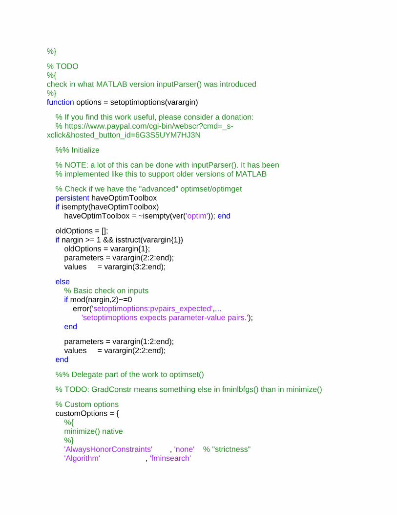
% TODO
%{
check in what MATLAB version inputParser() was introduced
%}
function options = setoptimoptions(varargin)
% If you find this work useful, please consider a donation: % https://www.paypal.com/cgi-bin/webscr?cmd=_s-xclick&hosted_button_id=6G3S5UYM7HJ3N
%% Initialize
% NOTE: a lot of this can be done with inputParser(). It has been % implemented like this to support older versions of MATLAB % Check if we have the "advanced" optimset/optimget persistent haveOptimToolbox
if isempty(haveOptimToolbox)
haveOptimToolbox = ~isempty(ver('optim')); end
oldOptions = []; if nargin >= 1 && isstruct(varargin{1})
oldOptions = varargin{1}; parameters = varargin(2:2:end); values = varargin(3:2:end); else % Basic check on inputs
if mod(nargin,2)~=0
error('setoptimoptions:pvpairs_expected',... 'setoptimoptions expects parameter-value pairs.'); end
parameters = varargin(1:2:end); values = varargin(2:2:end); end
%% Delegate part of the work to optimset()
% TODO: GradConstr means something else in fminlbfgs() than in minimize()
% Custom options
customOptions = {
%{
minimize() native
%}
'AlwaysHonorConstraints' , 'none' % "strictness"
'Algorithm' , 'fminsearch'
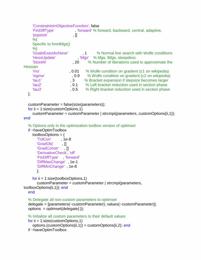
'ConstraintsInObjectiveFunction', false
'FinDiffType' , 'forward' % forward, backward, central, adaptive, 'popsize' , [] %{
Specific to fminlbfgs()
%}
'GoalsExactAchieve' , 1 % Normal line search with Wolfe conditions
'HessUpdate' , 'bfgs' % bfgs, lbfgs, steepdesc
'StoreN' , 20 % Number of itterations used to approximate the Hessian
'rho' , 0.01 % Wolfe condition on gradient (c1 on wikipedia)
'sigma' , 0.9 % Wolfe condition on gradient (c2 on wikipedia)
'tau1' , 3 % Bracket expansion if stepsize becomes larger
'tau2' , 0.1 % Left bracket reduction used in section phase
'tau3' , 0.5 % Right bracket reduction used in section phase
}; customParameter = false(size(parameters)); for ii = 1:size(customOptions,1)
customParameter = customParameter | strcmpi(parameters, customOptions{ii,1}); end
% Options only in the optimization toolbox version of optimset if ~haveOptimToolbox
toolboxOptions = {
'TolCon' , 1e-8
'GradObj' , [] 'GradConstr' , [] 'DerivativeCheck', 'off' 'FinDiffType' , 'forward' 'DiffMaxChange' , 1e-1
'DiffMinChange' , 1e-8
}; for ii = 1:size(toolboxOptions,1)
customParameter = customParameter | strcmpi(parameters, toolboxOptions{ii,1}); end
end
% Delegate all non-custom parameters to optimset delegate = [parameters(~customParameter); values(~customParameter)];
options = optimset(delegate{:}); % Initialize all custom parameters to their default values
for ii = 1:size(customOptions,1)
options.(customOptions{ii,1}) = customOptions{ii,2}; end
if ~haveOptimToolbox

for ii = 1:size(toolboxOptions,1)
options.(toolboxOptions{ii,1}) = toolboxOptions{ii,2}; end
end
% Merge any old options with new ones
if ~isempty(oldOptions)
fOld = fieldnames(oldOptions); % Custom options
for ii = 1:numel(customOptions(:,1))
if ~any(strcmpi(parameters, customOptions{ii,1})) && isfield(oldOptions, customOptions{ii,1}) && ~isempty(oldOptions.(customOptions{ii,1}))
options.(customOptions{ii,1}) = oldOptions.(customOptions{ii,1});
fOld(strcmpi(fOld,customOptions{ii,1})) = []; end
end
% Toolbox options
if ~haveOptimToolbox
for ii = 1:numel(toolboxOptions(:,1))
if ~any(strcmpi(parameters, toolboxOptions{ii,1})) && isfield(oldOptions, toolboxOptions{ii,1}) && ~isempty(oldOptions.(toolboxOptions{ii,1}))
options.(toolboxOptions{ii,1}) = oldOptions.(toolboxOptions{ii,1});
fOld(strcmpi(fOld,toolboxOptions{ii,1})) = []; end
end
end
% All other options
if ~isempty(fOld)
for ii = 1:numel(fOld) if ~any(strcmpi(parameters, fOld{ii})) && isfield(oldOptions, fOld{ii}) && ~isempty(oldOptions.(fOld{ii}))
options.(fOld{ii}) = oldOptions.(fOld{ii}); end
end
end
end
%% Parse the PV-pairs % The remainder
parameters = parameters(customParameter); values = values(customParameter); if ~isempty(parameters)
for ii = 1:numel(parameters)
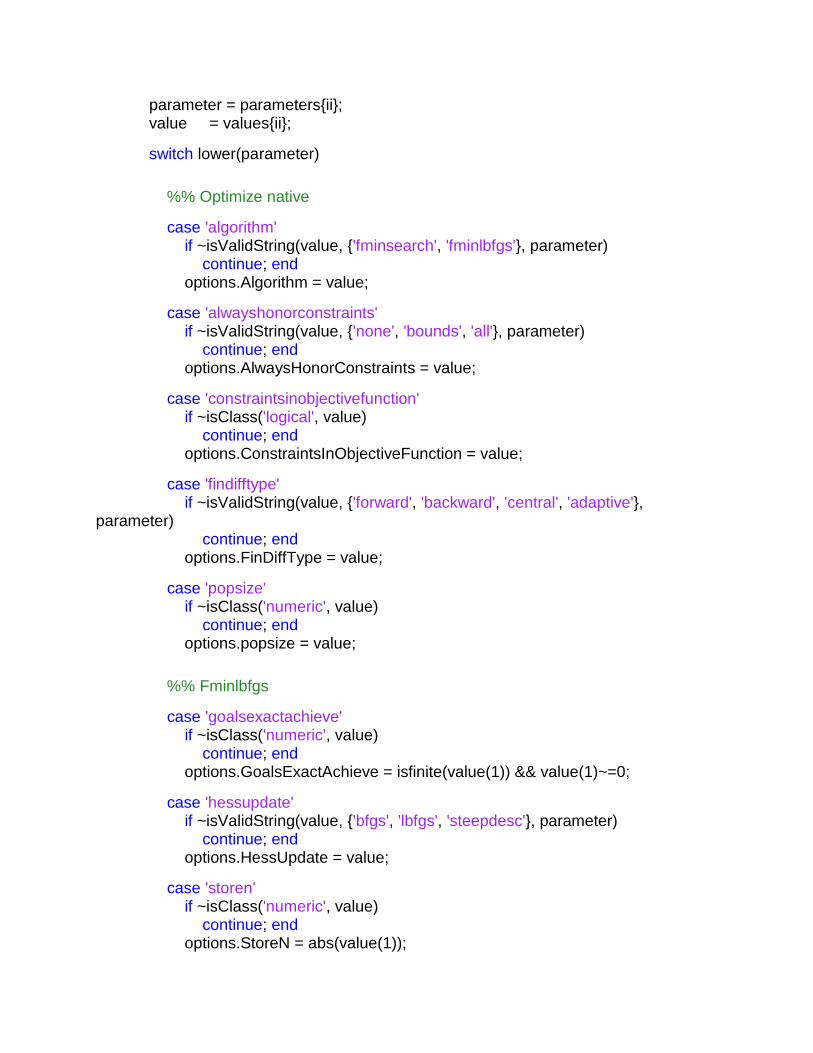
parameter = parameters{ii}; value = values{ii}; switch lower(parameter)
%% Optimize native
case 'algorithm' if ~isValidString(value, {'fminsearch', 'fminlbfgs'}, parameter)
continue; end
options.Algorithm = value; case 'alwayshonorconstraints' if ~isValidString(value, {'none', 'bounds', 'all'}, parameter)
continue; end
options.AlwaysHonorConstraints = value; case 'constraintsinobjectivefunction' if ~isClass('logical', value)
continue; end
options.ConstraintsInObjectiveFunction = value; case 'findifftype' if ~isValidString(value, {'forward', 'backward', 'central', 'adaptive'}, parameter)
continue; end options.FinDiffType = value; case 'popsize' if ~isClass('numeric', value)
continue; end
options.popsize = value; %% Fminlbfgs
case 'goalsexactachieve' if ~isClass('numeric', value)
continue; end
options.GoalsExactAchieve = isfinite(value(1)) && value(1)~=0; case 'hessupdate' if ~isValidString(value, {'bfgs', 'lbfgs', 'steepdesc'}, parameter)
continue; end
options.HessUpdate = value; case 'storen' if ~isClass('numeric', value)
continue; end
options.StoreN = abs(value(1));
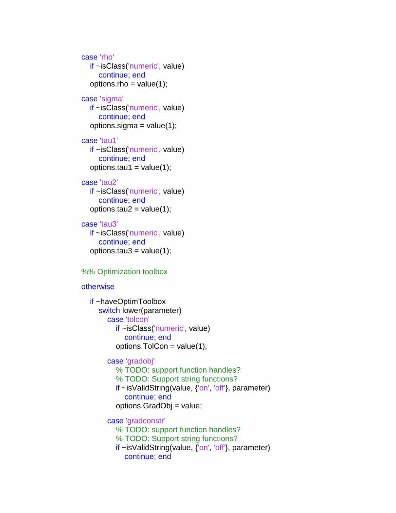
case 'rho' if ~isClass('numeric', value)
continue; end
options.rho = value(1); case 'sigma' if ~isClass('numeric', value)
continue; end
options.sigma = value(1); case 'tau1' if ~isClass('numeric', value)
continue; end
options.tau1 = value(1); case 'tau2' if ~isClass('numeric', value)
continue; end
options.tau2 = value(1); case 'tau3' if ~isClass('numeric', value)
continue; end
options.tau3 = value(1); %% Optimization toolbox
otherwise
if ~haveOptimToolbox
switch lower(parameter)
case 'tolcon' if ~isClass('numeric', value)
continue; end
options.TolCon = value(1); case 'gradobj' % TODO: support function handles?
% TODO: Support string functions?
if ~isValidString(value, {'on', 'off'}, parameter)
continue; end
options.GradObj = value; case 'gradconstr' % TODO: support function handles?
% TODO: Support string functions?
if ~isValidString(value, {'on', 'off'}, parameter)
continue; end
options.GradConstr = value; case 'derivativecheck' if ~isValidString(value, {'yes', 'no'}, parameter)
continue; end
% TODO: valid strings
options.DerivativeCheck = value; case 'findifftype' if ~isValidString(value, {'central', 'forward', 'backward'}, parameter)
continue; end
options.FinDiffType = value; case 'diffmaxchange' if ~isClass('numeric', value)
continue; end
options.DiffMaxChange = value(1); case 'diffminchange' if ~isClass('numeric', value)
continue; end
options.DiffMinChange = value(1); otherwise
warning(... 'setoptimoptions:unknown_option',... 'Unknown option: ''%s''. Ignoring...', parameter); continue
end
else
warning(... 'setoptimoptions:unknown_option',... 'Unknown option: ''%s''. Ignoring...', parameter); continue
end
end % switch
end % for
end % if end % function % Check if given string is one of the supported options. Generate
% appropriate warning messages if this is not the case. % NOTE: this is virtually the same as validatestring(), but this version
% can also be used on older versions of MATLAB function go_on = isValidString(received, validStrings, parameter)
go_on = true; if ~isClass('char', received)
go_on = false; return; end
if ~any(strcmpi(received, validStrings))
validStrings = [ cellfun(@(x) ['''' x ''', '], validStrings(1:end-1), 'UniformOutput', false),... ['and ''' validStrings(end) '''.'] ]; warning(... 'setoptimoptions:unsupported_value',... ['Unsupported option ''%s'' for parameter ''%s''.\n',... 'Valid options are: ' validStrings{:} '\nUsing default...'], ... received, parameter); go_on = false; end
end
% Check if class of given value is correct. Generate appropriate warning
% message if this is not the case. % NOTE: this is virtually the same as validateattributes(), but this % version can also be used on older versions of MATLAB function go_on = isClass(expected, received)
go_on = true; % More than one type may be allowable: if ischar(expected)
isCorrectClass = isa(received, expected); elseif iscell(expected) isCorrectClass = any(cellfun(@(x) isa(received, x), expected));
else
error(... 'setoptimoptions:BUG',... 'An internal error has occurred; please report this to the lead developer.'); end
% Generate warning if the type is not any of the supported ones
if ~isempty(received) && ~isCorrectClass
warning(... 'setoptimoptions:invalid_value',... 'Expected ''%s'', got ''%s''. Ignoring...', expected, class(received)); go_on = false;
end
end
% Check validity of file/function given as strnig
% NOTE: this functionality is deprecated, so a warning is ALWAYS issued. function [go_on, value] = checkFunction(value)
go_on = true; if ischar(value)
warning(... 'setoptimoptions:deprecated',... 'Using string functions or file names of MATLAB functions is deprecated; please use function_handles.'); if ~any(exist(value,'file')==[2 3 5 6])
warning(... 'setoptimoptions:invalid_script',... ['The file/function ''%s'' is invalid, or is not on the MATLAB search path.\n',... 'Using default...'], value); go_on = false; end
% Strip any extension, and convert to valid function handle
value = str2func(regexprep(value, '\.\w*$', '')); end
end
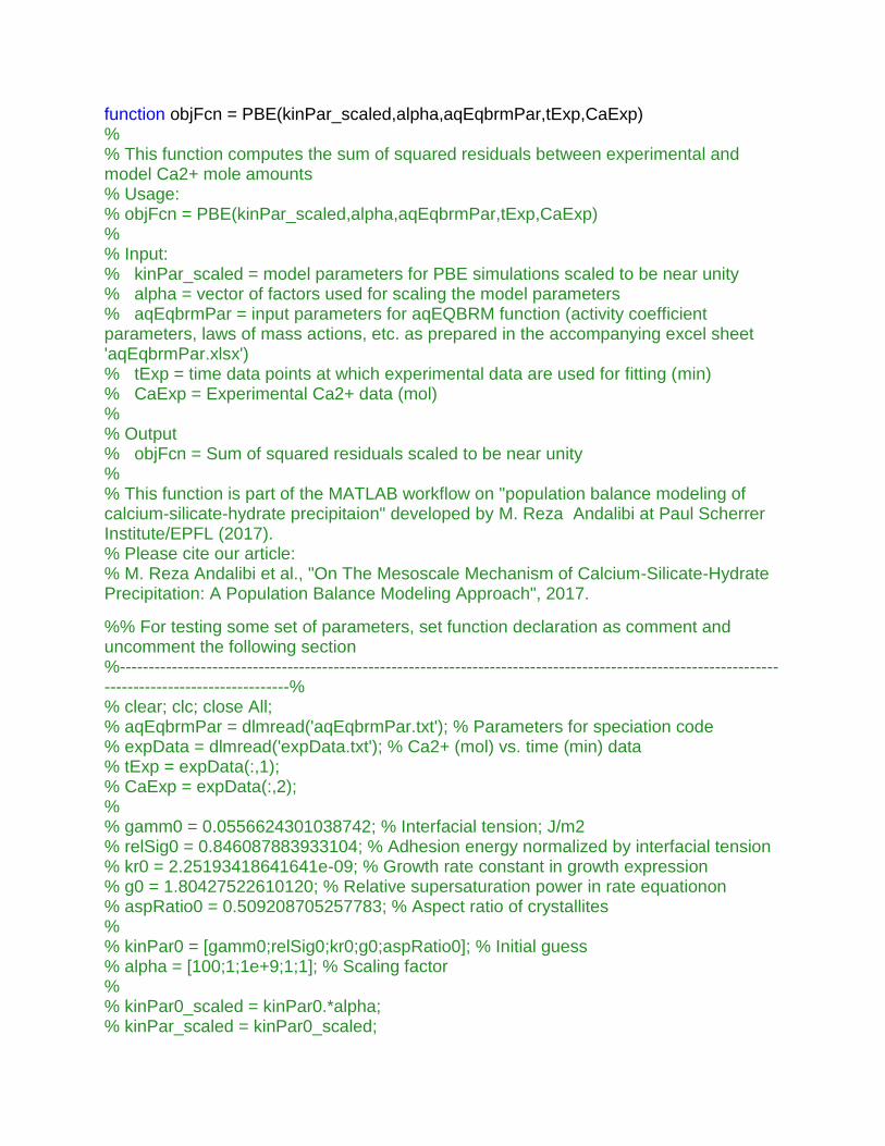
function objFcn = PBE(kinPar_scaled,alpha,aqEqbrmPar,tExp,CaExp)
% % This function computes the sum of squared residuals between experimental and model Ca2+ mole amounts
% Usage: % objFcn = PBE(kinPar_scaled,alpha,aqEqbrmPar,tExp,CaExp)
% % Input: % kinPar_scaled = model parameters for PBE simulations scaled to be near unity
% alpha = vector of factors used for scaling the model parameters
% aqEqbrmPar = input parameters for aqEQBRM function (activity coefficient parameters, laws of mass actions, etc. as prepared in the accompanying excel sheet 'aqEqbrmPar.xlsx')
% tExp = time data points at which experimental data are used for fitting (min)
% CaExp = Experimental Ca2+ data (mol)
% % Output % objFcn = Sum of squared residuals scaled to be near unity
% % This function is part of the MATLAB workflow on "population balance modeling of calcium-silicate-hydrate precipitaion" developed by M. Reza Andalibi at Paul Scherrer Institute/EPFL (2017). % Please cite our article: % M. Reza Andalibi et al., "On The Mesoscale Mechanism of Calcium-Silicate-Hydrate Precipitation: A Population Balance Modeling Approach", 2017. %% For testing some set of parameters, set function declaration as comment and uncomment the following section
%--------------------------------------------------------------------------------------------------------------------------------------------------%
% clear; clc; close All; % aqEqbrmPar = dlmread('aqEqbrmPar.txt'); % Parameters for speciation code
% expData = dlmread('expData.txt'); % Ca2+ (mol) vs. time (min) data
% tExp = expData(:,1); % CaExp = expData(:,2); % % gamm0 = 0.0556624301038742; % Interfacial tension; J/m2
% relSig0 = 0.846087883933104; % Adhesion energy normalized by interfacial tension
% kr0 = 2.25193418641641e-09; % Growth rate constant in growth expression
% g0 = 1.80427522610120; % Relative supersaturation power in rate equationon
% aspRatio0 = 0.509208705257783; % Aspect ratio of crystallites
% % kinPar0 = [gamm0;relSig0;kr0;g0;aspRatio0]; % Initial guess
% alpha = [100;1;1e+9;1;1]; % Scaling factor
% % kinPar0_scaled = kinPar0.*alpha; % kinPar_scaled = kinPar0_scaled;
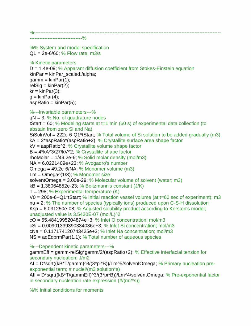
%--------------------------------------------------------------------------------------------------------------------------------------------------%
%% System and model specification
Q1 = 2e-6/60; % Flow rate; m3/s
% Kinetic parameters
D = 1.4e-09; % Apparant diffusion coefficient from Stokes-Einstein equation
kinPar = kinPar_scaled./alpha; gamm = kinPar(1); relSig = kinPar(2); kr = kinPar(3); g = kinPar(4); aspRatio = kinPar(5); %---Invariable parameters---%
qN = 3; % No. of quadrature nodes
tStart = 60; % Modeling starts at t=1 min (60 s) of experimental data collection (to abstain from zero Si and Na)
SiSolnVol = 222e-6-Q1*tStart; % Total volume of Si solution to be added gradually (m3)
kA = 2*aspRatio*(aspRatio+2); % Crystallite surface area shape factor
kV = aspRatio^2; % Crystallite volume shape factor
B = 4*kA^3/27/kV^2; % Crystallite shape factor
rhoMolar = 1/49.2e-6; % Solid molar density (mol/m3)
NA = 6.0221409e+23; % Avogadro's number
Omega = 49.2e-6/NA; % Monomer volume (m3)
Lm = Omega^(1/3); % Monomer size
solventOmega = 3.00e-29; % Molecular volume of solvent (water; m3)
kB = 1.38064852e-23; % Boltzmann's constant (J/K)
T = 298; % Experimental temperature (K)
V0 = 200e-6+Q1*tStart; % Initial reaction vessel volume (at t=60 sec of experiment); m3
nu = 2; % The number of species (typically ions) produced upon C-S-H dissolution
Ksp = 6.031250e-08; % Adjusted solubility product according to Kersten's model; unadjusted value is 3.5420E-07 (mol/L)^2
cO = 55.4841995204874e+3; % Inlet O concentration; mol/m3
cSi = 0.00901339390334036e+3; % Inlet Si concentration; mol/m3
cNa = 0.117174120743425e+3; % Inlet Na concentration; mol/m3
NS = aqEqbrmPar(1,1); % Total number of aqueous species
%---Dependent kinetic parameters---%
gammEff = gamm-relSig*gamm/2/(aspRatio+2); % Effective interfacial tension for secondary nucleation; J/m2
AI = D*sqrt((kB*T/gamm)^3/(3*pi*B))/Lm^5/solventOmega; % Primary nucleation pre-exponential term; # nuclei/(m3 solution*s)
AII = D*sqrt((kB*T/gammEff)^3/(3*pi*B))/Lm^4/solventOmega; % Pre-exponential factor in secondary nucleation rate expression (#/(m2*s))
%% Initial conditions for moments
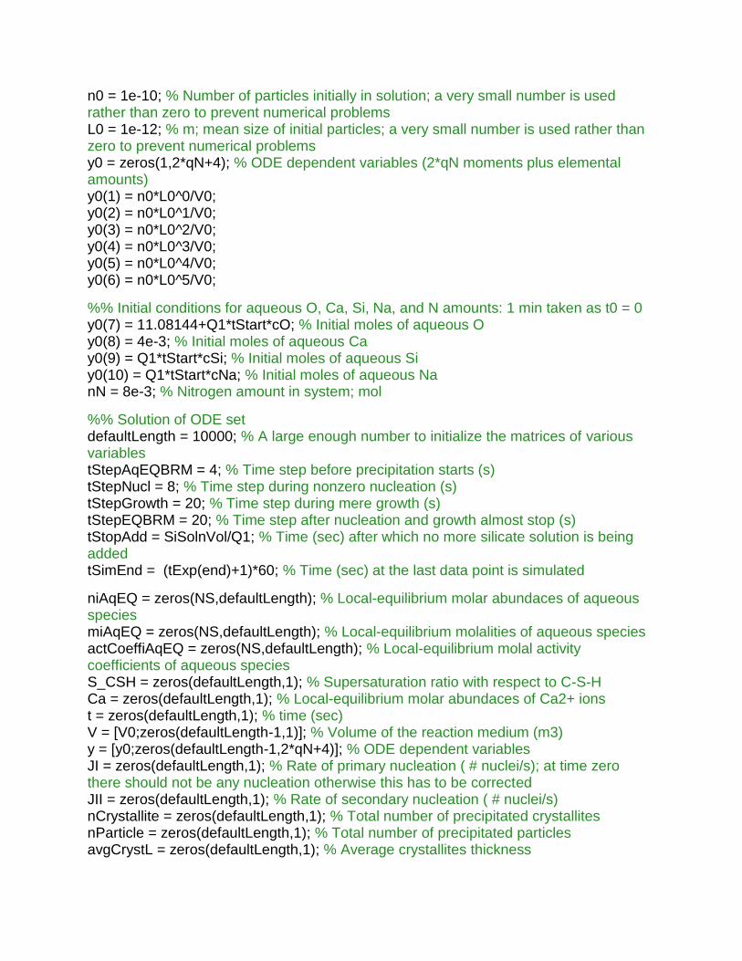
n0 = 1e-10; % Number of particles initially in solution; a very small number is used rather than zero to prevent numerical problems
L0 = 1e-12; % m; mean size of initial particles; a very small number is used rather than zero to prevent numerical problems
y0 = zeros(1,2*qN+4); % ODE dependent variables (2*qN moments plus elemental amounts)
y0(1) = n0*L0^0/V0; y0(2) = n0*L0^1/V0; y0(3) = n0*L0^2/V0; y0(4) = n0*L0^3/V0; y0(5) = n0*L0^4/V0; y0(6) = n0*L0^5/V0; %% Initial conditions for aqueous O, Ca, Si, Na, and N amounts: 1 min taken as t0 = 0
y0(7) = 11.08144+Q1*tStart*cO; % Initial moles of aqueous O
y0(8) = 4e-3; % Initial moles of aqueous Ca
y0(9) = Q1*tStart*cSi; % Initial moles of aqueous Si y0(10) = Q1*tStart*cNa; % Initial moles of aqueous Na
nN = 8e-3; % Nitrogen amount in system; mol %% Solution of ODE set defaultLength = 10000; % A large enough number to initialize the matrices of various variables
tStepAqEQBRM = 4; % Time step before precipitation starts (s)
tStepNucl = 8; % Time step during nonzero nucleation (s)
tStepGrowth = 20; % Time step during mere growth (s)
tStepEQBRM = 20; % Time step after nucleation and growth almost stop (s)
tStopAdd = SiSolnVol/Q1; % Time (sec) after which no more silicate solution is being added
tSimEnd = (tExp(end)+1)*60; % Time (sec) at the last data point is simulated
niAqEQ = zeros(NS,defaultLength); % Local-equilibrium molar abundaces of aqueous species
miAqEQ = zeros(NS,defaultLength); % Local-equilibrium molalities of aqueous species
actCoeffiAqEQ = zeros(NS,defaultLength); % Local-equilibrium molal activity coefficients of aqueous species
S_CSH = zeros(defaultLength,1); % Supersaturation ratio with respect to C-S-H
Ca = zeros(defaultLength,1); % Local-equilibrium molar abundaces of Ca2+ ions
t = zeros(defaultLength,1); % time (sec)
V = [V0;zeros(defaultLength-1,1)]; % Volume of the reaction medium (m3)
y = [y0;zeros(defaultLength-1,2*qN+4)]; % ODE dependent variables
JI = zeros(defaultLength,1); % Rate of primary nucleation ( # nuclei/s); at time zero there should not be any nucleation otherwise this has to be corrected
JII = zeros(defaultLength,1); % Rate of secondary nucleation ( # nuclei/s)
nCrystallite = zeros(defaultLength,1); % Total number of precipitated crystallites
nParticle = zeros(defaultLength,1); % Total number of precipitated particles
avgCrystL = zeros(defaultLength,1); % Average crystallites thickness
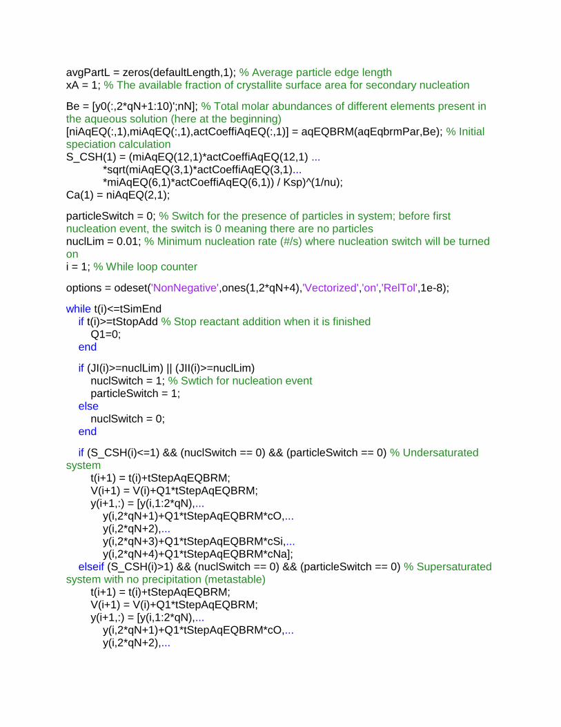
avgPartL = zeros(defaultLength,1); % Average particle edge length
xA = 1; % The available fraction of crystallite surface area for secondary nucleation
Be = [y0(:,2*qN+1:10)';nN]; % Total molar abundances of different elements present in the aqueous solution (here at the beginning)
[niAqEQ(:,1),miAqEQ(:,1),actCoeffiAqEQ(:,1)] = aqEQBRM(aqEqbrmPar,Be); % Initial speciation calculation
S_CSH(1) = (miAqEQ(12,1)*actCoeffiAqEQ(12,1) ... *sqrt(miAqEQ(3,1)*actCoeffiAqEQ(3,1)... *miAqEQ(6,1)*actCoeffiAqEQ(6,1)) / Ksp)^(1/nu); Ca(1) = niAqEQ(2,1); particleSwitch = 0; % Switch for the presence of particles in system; before first nucleation event, the switch is 0 meaning there are no particles
nuclLim = 0.01; % Minimum nucleation rate (#/s) where nucleation switch will be turned on
i = 1; % While loop counter
options = odeset('NonNegative',ones(1,2*qN+4),'Vectorized','on','RelTol',1e-8); while t(i)<=tSimEnd
if t(i)>=tStopAdd % Stop reactant addition when it is finished
Q1=0; end
if (JI(i)>=nuclLim) || (JII(i)>=nuclLim)
nuclSwitch = 1; % Swtich for nucleation event particleSwitch = 1; else
nuclSwitch = 0; end
if (S_CSH(i)<=1) && (nuclSwitch == 0) && (particleSwitch == 0) % Undersaturated system
t(i+1) = t(i)+tStepAqEQBRM; V(i+1) = V(i)+Q1*tStepAqEQBRM; y(i+1,:) = [y(i,1:2*qN),... y(i,2*qN+1)+Q1*tStepAqEQBRM*cO,... y(i,2*qN+2),... y(i,2*qN+3)+Q1*tStepAqEQBRM*cSi,... y(i,2*qN+4)+Q1*tStepAqEQBRM*cNa]; elseif (S_CSH(i)>1) && (nuclSwitch == 0) && (particleSwitch == 0) % Supersaturated system with no precipitation (metastable)
t(i+1) = t(i)+tStepAqEQBRM; V(i+1) = V(i)+Q1*tStepAqEQBRM; y(i+1,:) = [y(i,1:2*qN),... y(i,2*qN+1)+Q1*tStepAqEQBRM*cO,... y(i,2*qN+2),...
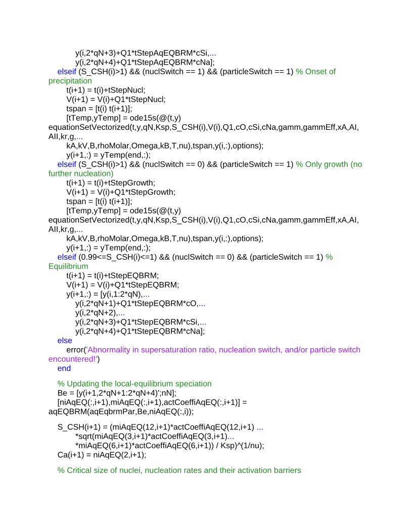
y(i,2*qN+3)+Q1*tStepAqEQBRM*cSi,... y(i,2*qN+4)+Q1*tStepAqEQBRM*cNa]; elseif (S_CSH(i)>1) && (nuclSwitch == 1) && (particleSwitch == 1) % Onset of precipitation
t(i+1) = t(i)+tStepNucl; V(i+1) = V(i)+Q1*tStepNucl; tspan = [t(i) t(i+1)]; [tTemp,yTemp] = ode15s(@(t,y) equationSetVectorized(t,y,qN,Ksp,S_CSH(i),V(i),Q1,cO,cSi,cNa,gamm,gammEff,xA,AI,AII,kr,g,... kA,kV,B,rhoMolar,Omega,kB,T,nu),tspan,y(i,:),options); y(i+1,:) = yTemp(end,:); elseif (S_CSH(i)>1) && (nuclSwitch == 0) && (particleSwitch == 1) % Only growth (no further nucleation)
t(i+1) = t(i)+tStepGrowth; V(i+1) = V(i)+Q1*tStepGrowth; tspan = [t(i) t(i+1)]; [tTemp,yTemp] = ode15s(@(t,y) equationSetVectorized(t,y,qN,Ksp,S_CSH(i),V(i),Q1,cO,cSi,cNa,gamm,gammEff,xA,AI,AII,kr,g,... kA,kV,B,rhoMolar,Omega,kB,T,nu),tspan,y(i,:),options); y(i+1,:) = yTemp(end,:); elseif (0.99<=S_CSH(i)<=1) && (nuclSwitch == 0) && (particleSwitch == 1) % Equilibrium
t(i+1) = t(i)+tStepEQBRM; V(i+1) = V(i)+Q1*tStepEQBRM; y(i+1,:) = [y(i,1:2*qN),... y(i,2*qN+1)+Q1*tStepEQBRM*cO,... y(i,2*qN+2),... y(i,2*qN+3)+Q1*tStepEQBRM*cSi,... y(i,2*qN+4)+Q1*tStepEQBRM*cNa]; else
error('Abnormality in supersaturation ratio, nucleation switch, and/or particle switch encountered!')
end
% Updating the local-equilibrium speciation
Be = [y(i+1,2*qN+1:2*qN+4)';nN]; [niAqEQ(:,i+1),miAqEQ(:,i+1),actCoeffiAqEQ(:,i+1)] = aqEQBRM(aqEqbrmPar,Be,niAqEQ(:,i)); S_CSH(i+1) = (miAqEQ(12,i+1)*actCoeffiAqEQ(12,i+1) ... *sqrt(miAqEQ(3,i+1)*actCoeffiAqEQ(3,i+1)... *miAqEQ(6,i+1)*actCoeffiAqEQ(6,i+1)) / Ksp)^(1/nu); Ca(i+1) = niAqEQ(2,i+1); % Critical size of nuclei, nucleation rates and their activation barriers
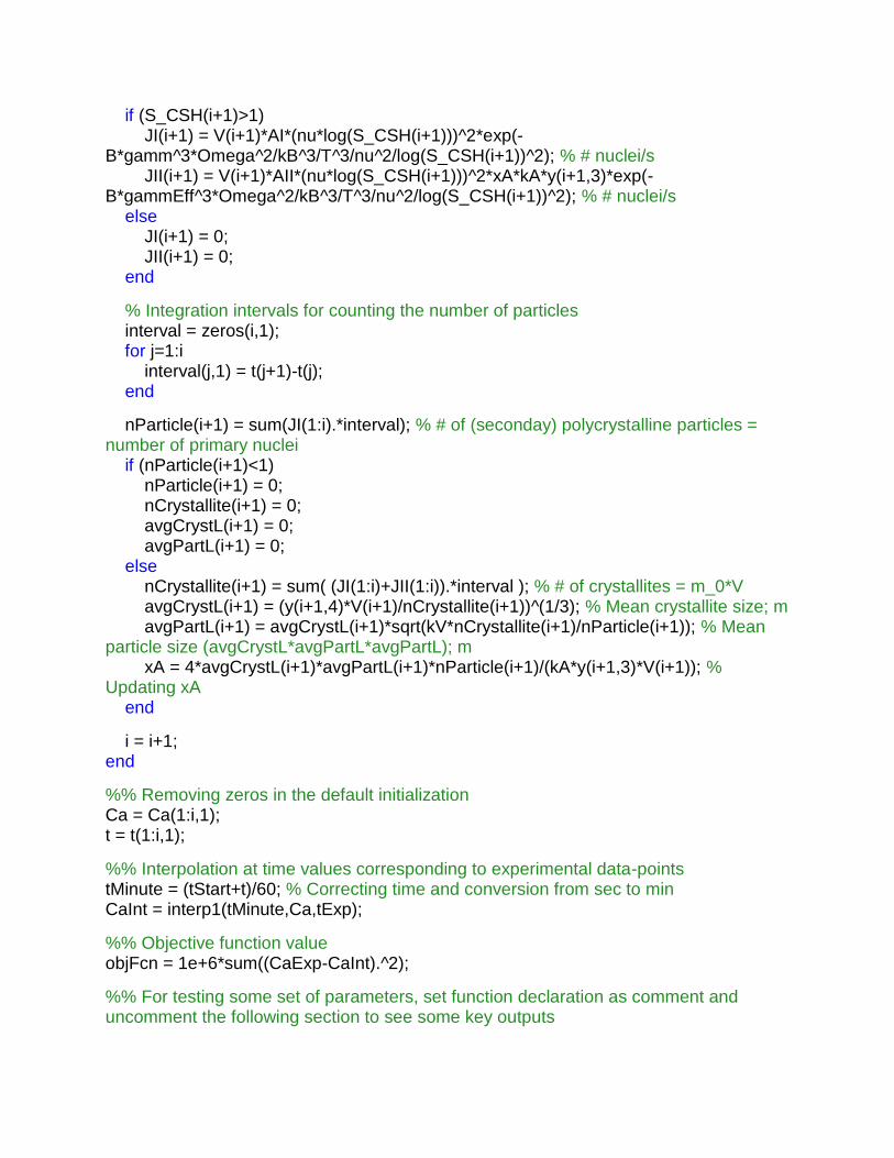
if (S_CSH(i+1)>1)
JI(i+1) = V(i+1)*AI*(nu*log(S_CSH(i+1)))^2*exp(-B*gamm^3*Omega^2/kB^3/T^3/nu^2/log(S_CSH(i+1))^2); % # nuclei/s
JII(i+1) = V(i+1)*AII*(nu*log(S_CSH(i+1)))^2*xA*kA*y(i+1,3)*exp(-B*gammEff^3*Omega^2/kB^3/T^3/nu^2/log(S_CSH(i+1))^2); % # nuclei/s
else
JI(i+1) = 0; JII(i+1) = 0; end
% Integration intervals for counting the number of particles
interval = zeros(i,1); for j=1:i interval(j,1) = t(j+1)-t(j); end
nParticle(i+1) = sum(JI(1:i).*interval); % # of (seconday) polycrystalline particles = number of primary nuclei if (nParticle(i+1)<1)
nParticle(i+1) = 0; nCrystallite(i+1) = 0; avgCrystL(i+1) = 0; avgPartL(i+1) = 0; else
nCrystallite(i+1) = sum( (JI(1:i)+JII(1:i)).*interval ); % # of crystallites = m_0*V
avgCrystL(i+1) = (y(i+1,4)*V(i+1)/nCrystallite(i+1))^(1/3); % Mean crystallite size; m
avgPartL(i+1) = avgCrystL(i+1)*sqrt(kV*nCrystallite(i+1)/nParticle(i+1)); % Mean particle size (avgCrystL*avgPartL*avgPartL); m
xA = 4*avgCrystL(i+1)*avgPartL(i+1)*nParticle(i+1)/(kA*y(i+1,3)*V(i+1)); % Updating xA
end
i = i+1; end
%% Removing zeros in the default initialization
Ca = Ca(1:i,1); t = t(1:i,1); %% Interpolation at time values corresponding to experimental data-points
tMinute = (tStart+t)/60; % Correcting time and conversion from sec to min
CaInt = interp1(tMinute,Ca,tExp); %% Objective function value
objFcn = 1e+6*sum((CaExp-CaInt).^2); %% For testing some set of parameters, set function declaration as comment and uncomment the following section to see some key outputs

%--------------------------------------------------------------------------------------------------------------------------------------------------%
% fig = fig('Name','Fitted Ca2+ mole amounts','Color','white'); % ax = axes('Parent',fig); % plot(tExp,CaExp,'bo','MarkerSize',5); hold on; % plot(tExp,CaInt,'r-','LineWidth',2); % set(ax,'FontSize',22,'FontWeight','bold'); % % axis square
% xlabel('Time (min)')
% ylabel('Aqueous Ca2+ amount (mol)')
% hold off % avgCrystL = 1e+9*avgCrystL(1:i,1); % nm
% avgPartL = 1e+9*avgPartL(1:i,1); % nm
% avgCrystL(end)
% avgPartL(end)
% S_Port = sqrt( (miAqEQ(2,:).*actCoeffiAqEQ(2,:).*(miAqEQ(6,:).*actCoeffiAqEQ(6,:)).^2)/3.85080e-6 ); % max(S_Port)
%--------------------------------------------------------------------------------------------------------------------------------------------------%

function dydt = equationSetVectorized(t,y,qN,Ksp,S,V,Q1,cO,cSi,cNa,gamm,gammEff,xA,AI,AII,kr,g,avgCrystL,... kA,kV,B,rhoMolar,Omega,kB,T,nu)
% % This function generates the set of ODEs (PBE + mass balances) to be numerically solved for computational modeling of C-S-H precipitation % % Usage: % dydt = equationSetVectorized(t,y,qN,Ksp,S,V,Q1,cO,cSi,cNa,gamm,gammEff,xA,AI,AII,kr,g,avgCrystL,kA,kV,B,rhoMolar,Omega,kB,T,nu) % % Input: % t = Time; % y = Dependent variables (moments + elemental abundances)
% qN = No. of quadrature nodes
% Ksp = Adjusted solubility product according to Kersten's model; unadjusted value is 3.5420E-07 (mol/L)^2
% S = Supersaturation ratio
% V = System volume
% Q1 = Reactant flow rate
% cO = Inlet O concentration; mol/m3
% cSi = Inlet Si concentration; mol/m3
% cNa = Inlet Na concentration; mol/m3
% gamm = Interfacial tension
% gammEff = Effective interfacial tension for secondary nucleation
% xA = The available fraction of crystallite surface area for secondary nucleation
% AI = Primary nucleation pre-exponential term
% AII = Secondary nucleation pre-exponential term
% kr = Growth rate constant in growth expression
% g = Relative supersaturation power in rate equationon
% avgCrystL = Average crystallites thickness
% kA = Surface area shape factor
% kV = Volume shape factor
% B = Shape factor
% rhoMolar = Solid molar density
% Omega = Monomer volume
% kB = Boltzmann's constant % T = Temperature
% nu = The number of species produced upon C-S-H dissolution
% % Output: % dydt = ODE describing the respective dependent variable written in a vectorized manner
%
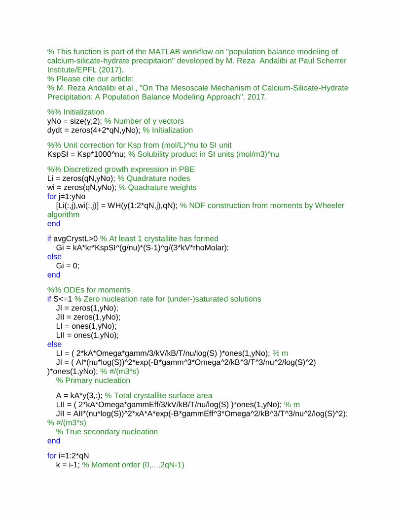
% This function is part of the MATLAB workflow on "population balance modeling of calcium-silicate-hydrate precipitaion" developed by M. Reza Andalibi at Paul Scherrer Institute/EPFL (2017). % Please cite our article: % M. Reza Andalibi et al., "On The Mesoscale Mechanism of Calcium-Silicate-Hydrate Precipitation: A Population Balance Modeling Approach", 2017. %% Initialization
yNo = size(y,2); % Number of y vectors
dydt = zeros(4+2*qN,yNo); % Initialization
%% Unit correction for Ksp from (mol/L)^nu to SI unit KspSI = Ksp*1000^nu; % Solubility product in SI units (mol/m3)^nu
%% Discretized growth expression in PBE
Li = zeros(qN,yNo); % Quadrature nodes
wi = zeros(qN,yNo); % Quadrature weights
for j=1:yNo
[Li(:,j),wi(:,j)] = WH(y(1:2*qN,j),qN); % NDF construction from moments by Wheeler algorithm
end
if avgCrystL>0 % At least 1 crystallite has formed
Gi = kA*kr*KspSI^(g/nu)*(S-1)^g/(3*kV*rhoMolar); else
Gi = 0; end
%% ODEs for moments
if S<=1 % Zero nucleation rate for (under-)saturated solutions
JI = zeros(1,yNo); JII = zeros(1,yNo); LI = ones(1,yNo); LII = ones(1,yNo); else
LI = ( 2*kA*Omega*gamm/3/kV/kB/T/nu/log(S) )*ones(1,yNo); % m
JI = ( AI*(nu*log(S))^2*exp(-B*gamm^3*Omega^2/kB^3/T^3/nu^2/log(S)^2) )*ones(1,yNo); % #/(m3*s)
% Primary nucleation
A = kA*y(3,:); % Total crystallite surface area
LII = ( 2*kA*Omega*gammEff/3/kV/kB/T/nu/log(S) )*ones(1,yNo); % m
JII = AII*(nu*log(S))^2*xA*A*exp(-B*gammEff^3*Omega^2/kB^3/T^3/nu^2/log(S)^2); % #/(m3*s)
% True secondary nucleation
end
for i=1:2*qN
k = i-1; % Moment order (0,...,2qN-1)

dydt(i,:) = -y(i,:)*Q1/V + k*sum(wi.*Gi.*Li.^(k-1),1) + JI.*LI.^k + JII.*LII.^k; end
%% ODEs for mass balances (O(aq), Ca(aq), Si(aq), and Na(aq), respectively)
dCSHdt = (3*sum((wi.*Gi.*Li.^2),1) + JI.*LI.^3 + JII.*LII.^3)*kV*V*rhoMolar; % Rate of CSH precipitation (mol/s)
dydt(2*qN+1,:) = Q1*cO-3.5*dCSHdt; % O
dydt(2*qN+2,:) = -dCSHdt; % Ca
dydt(2*qN+3,:) = Q1*cSi-0.5*dCSHdt; % Si dydt(2*qN+4,:) = Q1*cNa; % Na
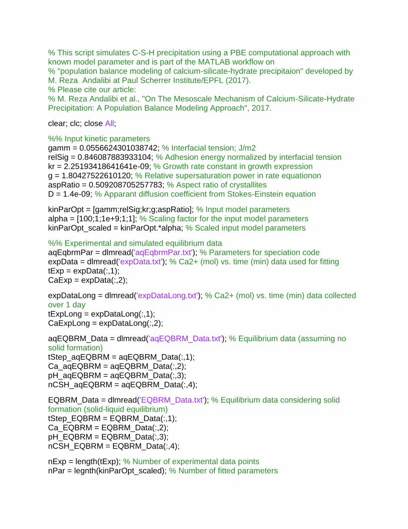
% This script simulates C-S-H precipitation using a PBE computational approach with known model parameter and is part of the MATLAB workflow on
% "population balance modeling of calcium-silicate-hydrate precipitaion" developed by M. Reza Andalibi at Paul Scherrer Institute/EPFL (2017). % Please cite our article: % M. Reza Andalibi et al., "On The Mesoscale Mechanism of Calcium-Silicate-Hydrate Precipitation: A Population Balance Modeling Approach", 2017. clear; clc; close All; %% Input kinetic parameters
gamm = 0.0556624301038742; % Interfacial tension; J/m2
relSig = 0.846087883933104; % Adhesion energy normalized by interfacial tension
kr = 2.25193418641641e-09; % Growth rate constant in growth expression
g = 1.80427522610120; % Relative supersaturation power in rate equationon
aspRatio = 0.509208705257783; % Aspect ratio of crystallites
D = 1.4e-09; % Apparant diffusion coefficient from Stokes-Einstein equation
kinParOpt = [gamm;relSig;kr;g;aspRatio]; % Input model parameters
alpha = [100;1;1e+9;1;1]; % Scaling factor for the input model parameters
kinParOpt_scaled = kinParOpt.*alpha; % Scaled input model parameters
%% Experimental and simulated equilibrium data
aqEqbrmPar = dlmread('aqEqbrmPar.txt'); % Parameters for speciation code
expData = dlmread('expData.txt'); % Ca2+ (mol) vs. time (min) data used for fitting
tExp = expData(:,1); CaExp = expData(:,2); expDataLong = dlmread('expDataLong.txt'); % Ca2+ (mol) vs. time (min) data collected over 1 day
tExpLong = expDataLong(:,1); CaExpLong = expDataLong(:,2); aqEQBRM_Data = dlmread('aqEQBRM_Data.txt'); % Equilibrium data (assuming no solid formation)
tStep_aqEQBRM = aqEQBRM_Data(:,1); Ca_aqEQBRM = aqEQBRM_Data(:,2); pH_aqEQBRM = aqEQBRM_Data(:,3); nCSH_aqEQBRM = aqEQBRM_Data(:,4); EQBRM_Data = dlmread('EQBRM_Data.txt'); % Equilibrium data considering solid formation (solid-liquid equilibrium)
tStep_EQBRM = EQBRM_Data(:,1); Ca_EQBRM = EQBRM_Data(:,2); pH_EQBRM = EQBRM_Data(:,3); nCSH_EQBRM = EQBRM_Data(:,4); nExp = length(tExp); % Number of experimental data points
nPar = legnth(kinParOpt_scaled); % Number of fitted parameters
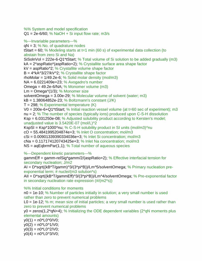
%% System and model specification
Q1 = 2e-6/60; % NaOH + Si input flow rate; m3/s
%---Invariable parameters---%
qN = 3; % No. of quadrature nodes
tStart = 60; % Modeling starts at t=1 min (60 s) of experimental data collection (to abstain from zero Si and Na)
SiSolnVol = 222e-6-Q1*tStart; % Total volume of Si solution to be added gradually (m3)
kA = 2*aspRatio*(aspRatio+2); % Crystallite surface area shape factor
kV = aspRatio^2; % Crystallite volume shape factor
B = 4*kA^3/27/kV^2; % Crystallite shape factor
rhoMolar = 1/49.2e-6; % Solid molar density (mol/m3)
NA = 6.0221409e+23; % Avogadro's number
Omega = 49.2e-6/NA; % Monomer volume (m3)
Lm = Omega^(1/3); % Monomer size
solventOmega = 3.00e-29; % Molecular volume of solvent (water; m3)
kB = 1.38064852e-23; % Boltzmann's constant (J/K)
T = 298; % Experimental temperature (K)
V0 = 200e-6+Q1*tStart; % Initial reaction vessel volume (at t=60 sec of experiment); m3
nu = 2; % The number of species (typically ions) produced upon C-S-H dissolution
Ksp = 6.031250e-08; % Adjusted solubility product according to Kersten's model; unadjusted value is 3.5420E-07 (mol/L)^2
KspSI = Ksp*1000^nu; % C-S-H solubility product in SI units (mol/m3)^nu
cO = 55.4841995204874e+3; % Inlet O concentration; mol/m3
cSi = 0.00901339390334036e+3; % Inlet Si concentration; mol/m3
cNa = 0.117174120743425e+3; % Inlet Na concentration; mol/m3
NS = aqEqbrmPar(1,1); % Total number of aqueous species
%---Dependent kinetic parameters---%
gammEff = gamm-relSig*gamm/2/(aspRatio+2); % Effective interfacial tension for secondary nucleation; J/m2
AI = D*sqrt((kB*T/gamm)^3/(3*pi*B))/Lm^5/solventOmega; % Primary nucleation pre-exponential term; # nuclei/(m3 solution*s)
AII = D*sqrt((kB*T/gammEff)^3/(3*pi*B))/Lm^4/solventOmega; % Pre-exponential factor in secondary nucleation rate expression (#/(m2*s))
%% Initial conditions for moments
n0 = 1e-10; % Number of particles initially in solution; a very small number is used rather than zero to prevent numerical problems
L0 = 1e-12; % m; mean size of initial particles; a very small number is used rather than zero to prevent numerical problems
y0 = zeros(1,2*qN+4); % Initializing the ODE dependent variables (2*qN moments plus elemental amounts)
y0(1) = n0*L0^0/V0; y0(2) = n0*L0^1/V0; y0(3) = n0*L0^2/V0; y0(4) = n0*L0^3/V0;
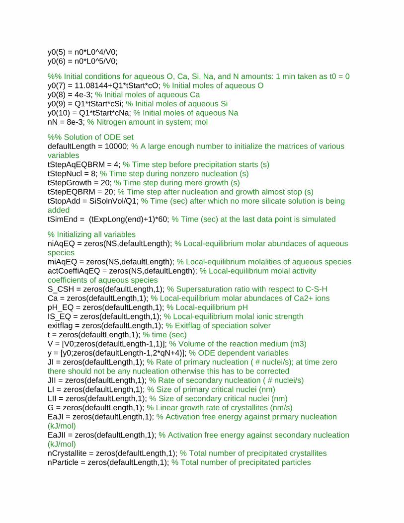
y0(5) = n0*L0^4/V0; y0(6) = n0*L0^5/V0; %% Initial conditions for aqueous O, Ca, Si, Na, and N amounts: 1 min taken as t0 = 0
y0(7) = 11.08144+Q1*tStart*cO; % Initial moles of aqueous O
y0(8) = 4e-3; % Initial moles of aqueous Ca
y0(9) = Q1*tStart*cSi; % Initial moles of aqueous Si y0(10) = Q1*tStart*cNa; % Initial moles of aqueous Na
nN = 8e-3; % Nitrogen amount in system; mol %% Solution of ODE set defaultLength = 10000; % A large enough number to initialize the matrices of various variables
tStepAqEQBRM = 4; % Time step before precipitation starts (s)
tStepNucl = 8; % Time step during nonzero nucleation (s)
tStepGrowth = 20; % Time step during mere growth (s)
tStepEQBRM = 20; % Time step after nucleation and growth almost stop (s)
tStopAdd = SiSolnVol/Q1; % Time (sec) after which no more silicate solution is being added
tSimEnd = (tExpLong(end)+1)*60; % Time (sec) at the last data point is simulated
% Initializing all variables
niAqEQ = zeros(NS,defaultLength); % Local-equilibrium molar abundaces of aqueous species
miAqEQ = zeros(NS,defaultLength); % Local-equilibrium molalities of aqueous species
actCoeffiAqEQ = zeros(NS,defaultLength); % Local-equilibrium molal activity coefficients of aqueous species
S_CSH = zeros(defaultLength,1); % Supersaturation ratio with respect to C-S-H
Ca = zeros(defaultLength,1); % Local-equilibrium molar abundaces of Ca2+ ions
pH_EQ = zeros(defaultLength,1); % Local-equilibrium pH
IS_EQ = zeros(defaultLength,1); % Local-equilibrium molal ionic strength
exitflag = zeros(defaultLength,1); % Exitflag of speciation solver
t = zeros(defaultLength,1); % time (sec)
V = [V0;zeros(defaultLength-1,1)]; % Volume of the reaction medium (m3)
y = [y0;zeros(defaultLength-1,2*qN+4)]; % ODE dependent variables
JI = zeros(defaultLength,1); % Rate of primary nucleation ( # nuclei/s); at time zero there should not be any nucleation otherwise this has to be corrected
JII = zeros(defaultLength,1); % Rate of secondary nucleation ( # nuclei/s)
LI = zeros(defaultLength,1); % Size of primary critical nuclei (nm)
LII = zeros(defaultLength,1); % Size of secondary critical nuclei (nm)
G = zeros(defaultLength,1); % Linear growth rate of crystallites (nm/s)
EaJI = zeros(defaultLength,1); % Activation free energy against primary nucleation (kJ/mol)
EaJII = zeros(defaultLength,1); % Activation free energy against secondary nucleation (kJ/mol)
nCrystallite = zeros(defaultLength,1); % Total number of precipitated crystallites
nParticle = zeros(defaultLength,1); % Total number of precipitated particles
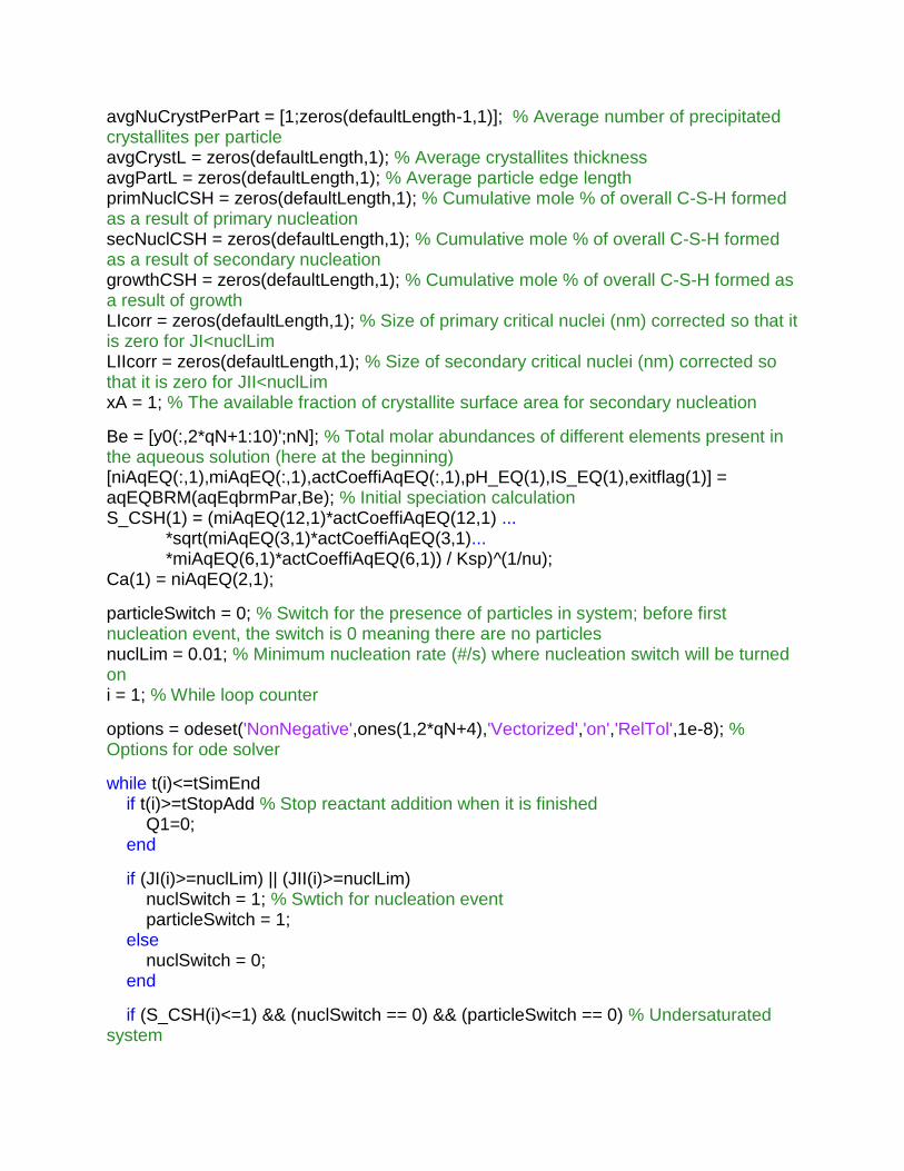
avgNuCrystPerPart = [1;zeros(defaultLength-1,1)]; % Average number of precipitated crystallites per particle
avgCrystL = zeros(defaultLength,1); % Average crystallites thickness
avgPartL = zeros(defaultLength,1); % Average particle edge length
primNuclCSH = zeros(defaultLength,1); % Cumulative mole % of overall C-S-H formed as a result of primary nucleation
secNuclCSH = zeros(defaultLength,1); % Cumulative mole % of overall C-S-H formed as a result of secondary nucleation
growthCSH = zeros(defaultLength,1); % Cumulative mole % of overall C-S-H formed as a result of growth
LIcorr = zeros(defaultLength,1); % Size of primary critical nuclei (nm) corrected so that it is zero for JI<nuclLim
LIIcorr = zeros(defaultLength,1); % Size of secondary critical nuclei (nm) corrected so that it is zero for JII<nuclLim
xA = 1; % The available fraction of crystallite surface area for secondary nucleation
Be = [y0(:,2*qN+1:10)';nN]; % Total molar abundances of different elements present in the aqueous solution (here at the beginning)
[niAqEQ(:,1),miAqEQ(:,1),actCoeffiAqEQ(:,1),pH_EQ(1),IS_EQ(1),exitflag(1)] = aqEQBRM(aqEqbrmPar,Be); % Initial speciation calculation
S_CSH(1) = (miAqEQ(12,1)*actCoeffiAqEQ(12,1) ... *sqrt(miAqEQ(3,1)*actCoeffiAqEQ(3,1)... *miAqEQ(6,1)*actCoeffiAqEQ(6,1)) / Ksp)^(1/nu); Ca(1) = niAqEQ(2,1); particleSwitch = 0; % Switch for the presence of particles in system; before first nucleation event, the switch is 0 meaning there are no particles
nuclLim = 0.01; % Minimum nucleation rate (#/s) where nucleation switch will be turned on
i = 1; % While loop counter
options = odeset('NonNegative',ones(1,2*qN+4),'Vectorized','on','RelTol',1e-8); % Options for ode solver
while t(i)<=tSimEnd
if t(i)>=tStopAdd % Stop reactant addition when it is finished
Q1=0; end
if (JI(i)>=nuclLim) || (JII(i)>=nuclLim)
nuclSwitch = 1; % Swtich for nucleation event particleSwitch = 1; else
nuclSwitch = 0; end
if (S_CSH(i)<=1) && (nuclSwitch == 0) && (particleSwitch == 0) % Undersaturated system
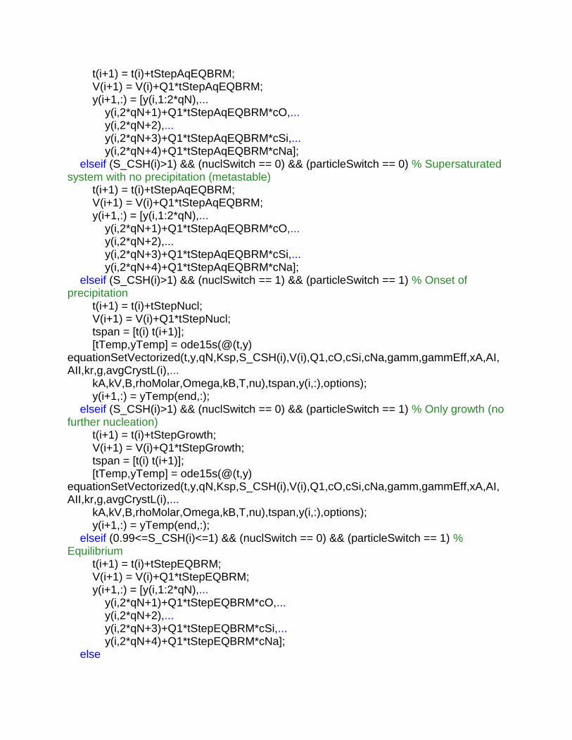
t(i+1) = t(i)+tStepAqEQBRM; V(i+1) = V(i)+Q1*tStepAqEQBRM; y(i+1,:) = [y(i,1:2*qN),... y(i,2*qN+1)+Q1*tStepAqEQBRM*cO,... y(i,2*qN+2),... y(i,2*qN+3)+Q1*tStepAqEQBRM*cSi,... y(i,2*qN+4)+Q1*tStepAqEQBRM*cNa]; elseif (S_CSH(i)>1) && (nuclSwitch == 0) && (particleSwitch == 0) % Supersaturated system with no precipitation (metastable)
t(i+1) = t(i)+tStepAqEQBRM; V(i+1) = V(i)+Q1*tStepAqEQBRM; y(i+1,:) = [y(i,1:2*qN),... y(i,2*qN+1)+Q1*tStepAqEQBRM*cO,... y(i,2*qN+2),... y(i,2*qN+3)+Q1*tStepAqEQBRM*cSi,... y(i,2*qN+4)+Q1*tStepAqEQBRM*cNa]; elseif (S_CSH(i)>1) && (nuclSwitch == 1) && (particleSwitch == 1) % Onset of precipitation
t(i+1) = t(i)+tStepNucl; V(i+1) = V(i)+Q1*tStepNucl; tspan = [t(i) t(i+1)]; [tTemp,yTemp] = ode15s(@(t,y) equationSetVectorized(t,y,qN,Ksp,S_CSH(i),V(i),Q1,cO,cSi,cNa,gamm,gammEff,xA,AI,AII,kr,g,avgCrystL(i),... kA,kV,B,rhoMolar,Omega,kB,T,nu),tspan,y(i,:),options); y(i+1,:) = yTemp(end,:); elseif (S_CSH(i)>1) && (nuclSwitch == 0) && (particleSwitch == 1) % Only growth (no further nucleation)
t(i+1) = t(i)+tStepGrowth; V(i+1) = V(i)+Q1*tStepGrowth; tspan = [t(i) t(i+1)]; [tTemp,yTemp] = ode15s(@(t,y) equationSetVectorized(t,y,qN,Ksp,S_CSH(i),V(i),Q1,cO,cSi,cNa,gamm,gammEff,xA,AI,AII,kr,g,avgCrystL(i),... kA,kV,B,rhoMolar,Omega,kB,T,nu),tspan,y(i,:),options); y(i+1,:) = yTemp(end,:); elseif (0.99<=S_CSH(i)<=1) && (nuclSwitch == 0) && (particleSwitch == 1) % Equilibrium
t(i+1) = t(i)+tStepEQBRM; V(i+1) = V(i)+Q1*tStepEQBRM; y(i+1,:) = [y(i,1:2*qN),... y(i,2*qN+1)+Q1*tStepEQBRM*cO,... y(i,2*qN+2),... y(i,2*qN+3)+Q1*tStepEQBRM*cSi,... y(i,2*qN+4)+Q1*tStepEQBRM*cNa]; else
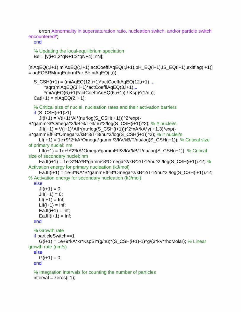
error('Abnormality in supersaturation ratio, nucleation switch, and/or particle switch encountered!')
end
% Updating the local-equilibrium speciation
Be = [y(i+1,2*qN+1:2*qN+4)';nN]; [niAqEQ(:,i+1),miAqEQ(:,i+1),actCoeffiAqEQ(:,i+1),pH_EQ(i+1),IS_EQ(i+1),exitflag(i+1)] = aqEQBRM(aqEqbrmPar,Be,niAqEQ(:,i)); S_CSH(i+1) = (miAqEQ(12,i+1)*actCoeffiAqEQ(12,i+1) ... *sqrt(miAqEQ(3,i+1)*actCoeffiAqEQ(3,i+1)... *miAqEQ(6,i+1)*actCoeffiAqEQ(6,i+1)) / Ksp)^(1/nu); Ca(i+1) = niAqEQ(2,i+1); % Critical size of nuclei, nucleation rates and their activation barriers
if (S_CSH(i+1)>1)
JI(i+1) = V(i+1)*AI*(nu*log(S_CSH(i+1)))^2*exp(-B*gamm^3*Omega^2/kB^3/T^3/nu^2/log(S_CSH(i+1))^2); % # nuclei/s
JII(i+1) = V(i+1)*AII*(nu*log(S_CSH(i+1)))^2*xA*kA*y(i+1,3)*exp(-B*gammEff^3*Omega^2/kB^3/T^3/nu^2/log(S_CSH(i+1))^2); % # nuclei/s
LI(i+1) = 1e+9*2*kA*Omega*gamm/3/kV/kB/T/nu/log(S_CSH(i+1)); % Critical size of primary nuclei; nm
LII(i+1) = 1e+9*2*kA*Omega*gammEff/3/kV/kB/T/nu/log(S_CSH(i+1)); % Critical size of secondary nuclei; nm
EaJI(i+1) = 1e-3*NA*B*gamm^3*Omega^2/kB^2/T^2/nu^2./log(S_CSH(i+1)).^2; % Activation energy for primary nucleation (kJ/mol)
EaJII(i+1) = 1e-3*NA*B*gammEff^3*Omega^2/kB^2/T^2/nu^2./log(S_CSH(i+1)).^2; % Activation energy for secondary nucleation (kJ/mol)
else
JI(i+1) = 0; JII(i+1) = 0; LI(i+1) = Inf; LII(i+1) = Inf; EaJI(i+1) = Inf; EaJII(i+1) = Inf; end
% Growth rate
if particleSwitch==1
G(i+1) = 1e+9*kA*kr*KspSI^(g/nu)*(S_CSH(i+1)-1)^g/(3*kV*rhoMolar); % Linear growth rate (nm/s)
else
G(i+1) = 0; end
% Integration intervals for counting the number of particles
interval = zeros(i,1);

for j=1:i interval(j,1) = t(j+1)-t(j); end
% Removing LI and LII values at nucleation rates smaller than nuclLim
if JI(i+1)<nuclLim
LIcorr(i+1)=0; else
LIcorr(i+1)=LI(i+1); end
if JII(i+1)<nuclLim
LIIcorr(i+1)=0; else
LIIcorr(i+1)=LII(i+1); end
nParticle(i+1) = sum(JI(1:i).*interval); % # of (seconday) polycrystalline particles = number of primary nuclei if (nParticle(i+1)<1)
nParticle(i+1) = 0; nCrystallite(i+1) = 0; avgNuCrystPerPart(i+1) = 0; avgCrystL(i+1) = 0; avgPartL(i+1) = 0; primNuclCSH(i+1) = 0; secNuclCSH(i+1) = 0; growthCSH(i+1) = 0; else
nCrystallite(i+1) = sum( (JI(1:i)+JII(1:i)).*interval ); % # of crystallites = m_0*V
avgNuCrystPerPart(i+1) = nCrystallite(i+1)/nParticle(i+1); % Average number of crystallites per particle
avgCrystL(i+1) = (y(i+1,4)*V(i+1)/nCrystallite(i+1))^(1/3); % Mean crystallite size; m
avgPartL(i+1) = avgCrystL(i+1)*sqrt(kV*nCrystallite(i+1)/nParticle(i+1)); % Mean particle size (avgCrystL*avgPartL*avgPartL); m
xA = 4*avgCrystL(i+1)*avgPartL(i+1)*nParticle(i+1)/(kA*y(i+1,3)*V(i+1)); % Updating xA
% Cumulative amounts of CSH precipitated as a result of various sub-
% processes normalized by the overall amount(%)
primNuclCSH(i+1) = 100*sum(JI(1:i).*interval.*LIcorr(1:i).^3*1e-27)/(y(i+1,4)*V(i+1)); % Precipitated CSH due to primary nucleation (mol); JI is in # nuclei/s
secNuclCSH(i+1) = 100*sum(JII(1:i).*interval.*LIIcorr(1:i).^3*1e-27)/(y(i+1,4)*V(i+1)); % Precipitated CSH due to secondary nucleation (mol); JII is in # nuclei/s
growthCSH(i+1) = 100-(primNuclCSH(i+1)+secNuclCSH(i+1)); % Precipitated CSH due to growth (mol); G is in nm/s
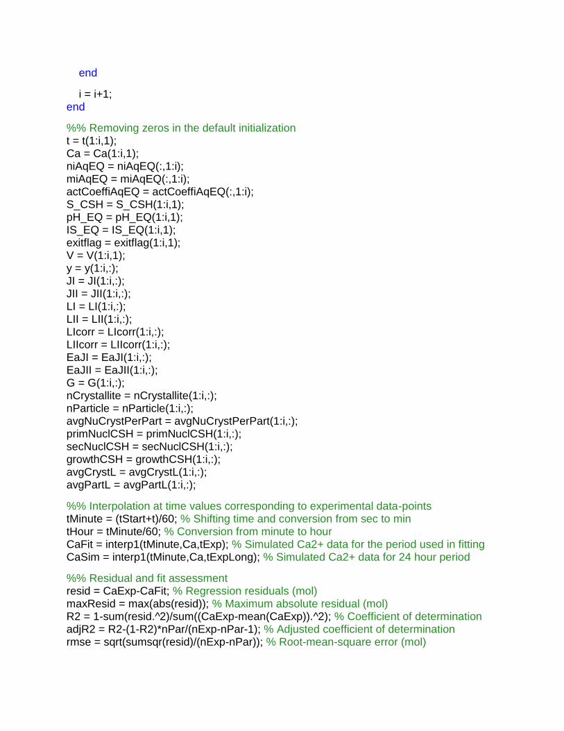
end
i = i+1; end
%% Removing zeros in the default initialization
t = t(1:i,1); Ca = Ca(1:i,1); niAqEQ = niAqEQ(:,1:i); miAqEQ = miAqEQ(:,1:i); actCoeffiAqEQ = actCoeffiAqEQ(:,1:i); S_CSH = S_CSH(1:i,1); pH_EQ = pH_EQ(1:i,1); IS_EQ = IS_EQ(1:i,1); exitflag = exitflag(1:i,1); V = V(1:i,1); y = y(1:i,:); JI = JI(1:i,:); JII = JII(1:i,:); LI = LI(1:i,:); LII = LII(1:i,:); LIcorr = LIcorr(1:i,:); LIIcorr = LIIcorr(1:i,:); EaJI = EaJI(1:i,:); EaJII = EaJII(1:i,:); G = G(1:i,:); nCrystallite = nCrystallite(1:i,:); nParticle = nParticle(1:i,:); avgNuCrystPerPart = avgNuCrystPerPart(1:i,:); primNuclCSH = primNuclCSH(1:i,:); secNuclCSH = secNuclCSH(1:i,:); growthCSH = growthCSH(1:i,:); avgCrystL = avgCrystL(1:i,:); avgPartL = avgPartL(1:i,:); %% Interpolation at time values corresponding to experimental data-points
tMinute = (tStart+t)/60; % Shifting time and conversion from sec to min
tHour = tMinute/60; % Conversion from minute to hour
CaFit = interp1(tMinute,Ca,tExp); % Simulated Ca2+ data for the period used in fitting
CaSim = interp1(tMinute,Ca,tExpLong); % Simulated Ca2+ data for 24 hour period
%% Residual and fit assessment resid = CaExp-CaFit; % Regression residuals (mol)
maxResid = max(abs(resid)); % Maximum absolute residual (mol)
R2 = 1-sum(resid.^2)/sum((CaExp-mean(CaExp)).^2); % Coefficient of determination
adjR2 = R2-(1-R2)*nPar/(nExp-nPar-1); % Adjusted coefficient of determination
rmse = sqrt(sumsqr(resid)/(nExp-nPar)); % Root-mean-square error (mol)
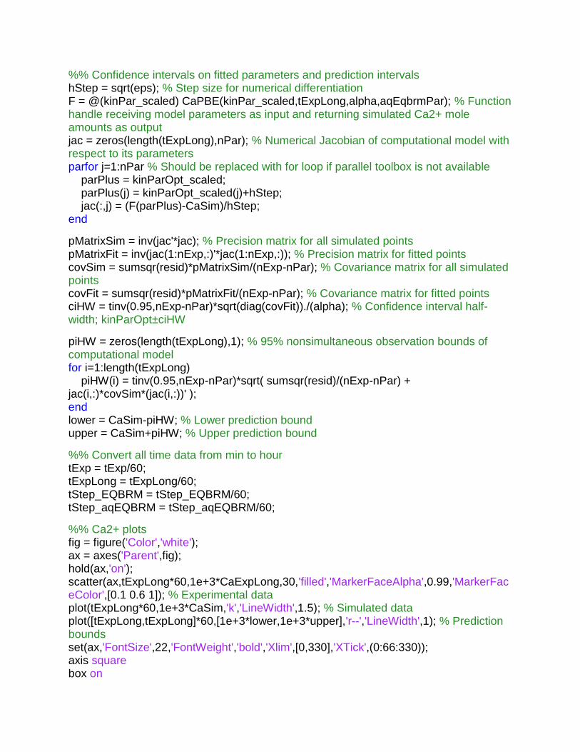
%% Confidence intervals on fitted parameters and prediction intervals
hStep = sqrt(eps); % Step size for numerical differentiation
F = @(kinPar_scaled) CaPBE(kinPar_scaled,tExpLong,alpha,aqEqbrmPar); % Function handle receiving model parameters as input and returning simulated Ca2+ mole amounts as output jac = zeros(length(tExpLong),nPar); % Numerical Jacobian of computational model with respect to its parameters
parfor j=1:nPar % Should be replaced with for loop if parallel toolbox is not available
parPlus = kinParOpt_scaled; parPlus(j) = kinParOpt_scaled(j)+hStep; jac(:,j) = (F(parPlus)-CaSim)/hStep; end
pMatrixSim = inv(jac'*jac); % Precision matrix for all simulated points
pMatrixFit = inv(jac(1:nExp,:)'*jac(1:nExp,:)); % Precision matrix for fitted points
covSim = sumsqr(resid)*pMatrixSim/(nExp-nPar); % Covariance matrix for all simulated points
covFit = sumsqr(resid)*pMatrixFit/(nExp-nPar); % Covariance matrix for fitted points
ciHW = tinv(0.95,nExp-nPar)*sqrt(diag(covFit))./(alpha); % Confidence interval half-width; kinParOpt±ciHW
piHW = zeros(length(tExpLong),1); % 95% nonsimultaneous observation bounds of computational model for i=1:length(tExpLong)
piHW(i) = tinv(0.95,nExp-nPar)*sqrt( sumsqr(resid)/(nExp-nPar) + jac(i,:)*covSim*(jac(i,:))' ); end
lower = CaSim-piHW; % Lower prediction bound
upper = CaSim+piHW; % Upper prediction bound
%% Convert all time data from min to hour
tExp = tExp/60; tExpLong = tExpLong/60; tStep_EQBRM = tStep_EQBRM/60; tStep_aqEQBRM = tStep_aqEQBRM/60; %% Ca2+ plots
fig = figure('Color','white'); ax = axes('Parent',fig); hold(ax,'on'); scatter(ax,tExpLong*60,1e+3*CaExpLong,30,'filled','MarkerFaceAlpha',0.99,'MarkerFaceColor',[0.1 0.6 1]); % Experimental data
plot(tExpLong*60,1e+3*CaSim,'k','LineWidth',1.5); % Simulated data
plot([tExpLong,tExpLong]*60,[1e+3*lower,1e+3*upper],'r--','LineWidth',1); % Prediction bounds
set(ax,'FontSize',22,'FontWeight','bold','Xlim',[0,330],'XTick',(0:66:330)); axis square
box on
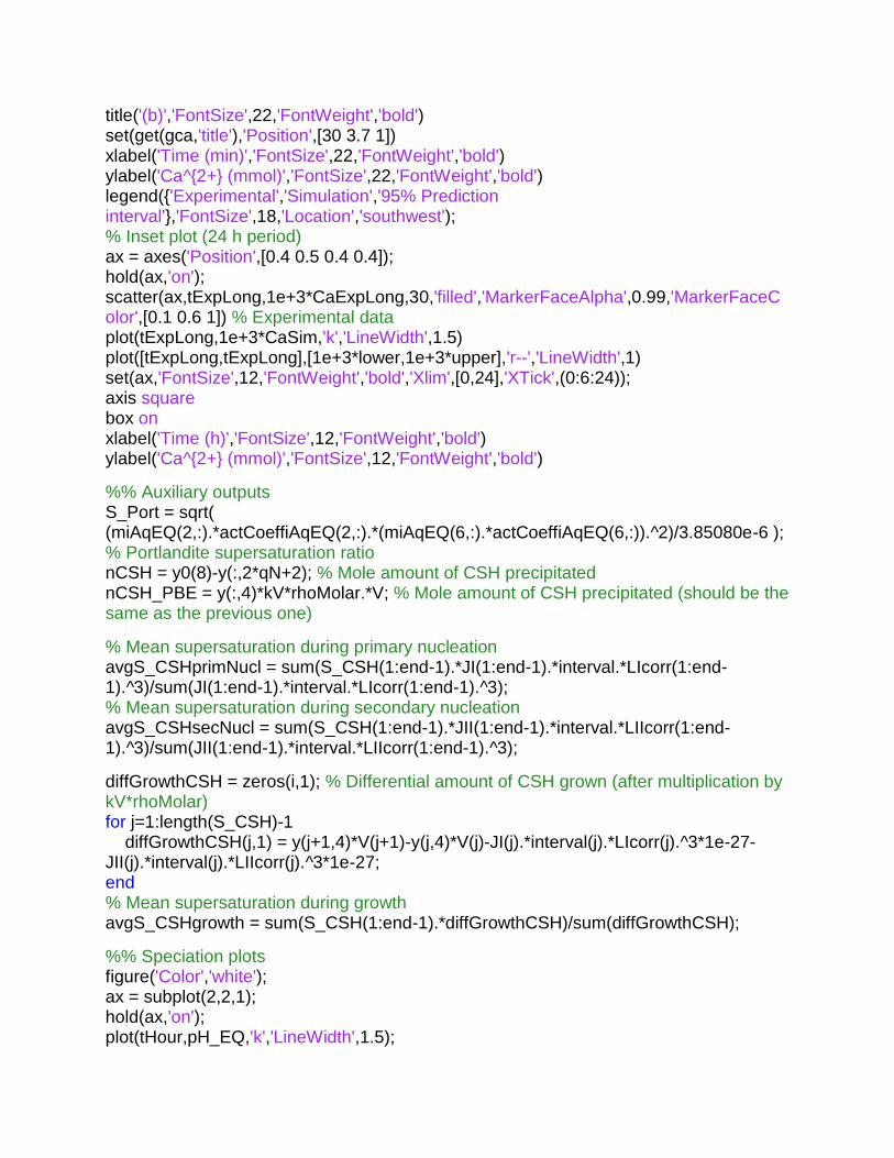
title('(b)','FontSize',22,'FontWeight','bold')
set(get(gca,'title'),'Position',[30 3.7 1])
xlabel('Time (min)','FontSize',22,'FontWeight','bold')
ylabel('Ca^{2+} (mmol)','FontSize',22,'FontWeight','bold')
legend({'Experimental','Simulation','95% Prediction interval'},'FontSize',18,'Location','southwest'); % Inset plot (24 h period)
ax = axes('Position',[0.4 0.5 0.4 0.4]); hold(ax,'on'); scatter(ax,tExpLong,1e+3*CaExpLong,30,'filled','MarkerFaceAlpha',0.99,'MarkerFaceColor',[0.1 0.6 1]) % Experimental data
plot(tExpLong,1e+3*CaSim,'k','LineWidth',1.5)
plot([tExpLong,tExpLong],[1e+3*lower,1e+3*upper],'r--','LineWidth',1)
set(ax,'FontSize',12,'FontWeight','bold','Xlim',[0,24],'XTick',(0:6:24)); axis square
box on
xlabel('Time (h)','FontSize',12,'FontWeight','bold')
ylabel('Ca^{2+} (mmol)','FontSize',12,'FontWeight','bold')
%% Auxiliary outputs
S_Port = sqrt( (miAqEQ(2,:).*actCoeffiAqEQ(2,:).*(miAqEQ(6,:).*actCoeffiAqEQ(6,:)).^2)/3.85080e-6 ); % Portlandite supersaturation ratio
nCSH = y0(8)-y(:,2*qN+2); % Mole amount of CSH precipitated
nCSH_PBE = y(:,4)*kV*rhoMolar.*V; % Mole amount of CSH precipitated (should be the same as the previous one)
% Mean supersaturation during primary nucleation
avgS_CSHprimNucl = sum(S_CSH(1:end-1).*JI(1:end-1).*interval.*LIcorr(1:end-1).^3)/sum(JI(1:end-1).*interval.*LIcorr(1:end-1).^3); % Mean supersaturation during secondary nucleation
avgS_CSHsecNucl = sum(S_CSH(1:end-1).*JII(1:end-1).*interval.*LIIcorr(1:end-1).^3)/sum(JII(1:end-1).*interval.*LIIcorr(1:end-1).^3); diffGrowthCSH = zeros(i,1); % Differential amount of CSH grown (after multiplication by kV*rhoMolar)
for j=1:length(S_CSH)-1
diffGrowthCSH(j,1) = y(j+1,4)*V(j+1)-y(j,4)*V(j)-JI(j).*interval(j).*LIcorr(j).^3*1e-27-JII(j).*interval(j).*LIIcorr(j).^3*1e-27; end
% Mean supersaturation during growth
avgS_CSHgrowth = sum(S_CSH(1:end-1).*diffGrowthCSH)/sum(diffGrowthCSH); %% Speciation plots
figure('Color','white'); ax = subplot(2,2,1); hold(ax,'on'); plot(tHour,pH_EQ,'k','LineWidth',1.5);
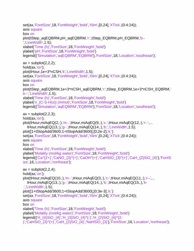
set(ax,'FontSize',18,'FontWeight','bold','Xlim',[0,24],'XTick',(0:4:24)); axis square
box on
plot(tStep_aqEQBRM,pH_aqEQBRM,'r:',tStep_EQBRM,pH_EQBRM,'b--','LineWidth',1.5); xlabel('Time (h)','FontSize',18,'FontWeight','bold')
ylabel('pH','FontSize',18,'FontWeight','bold')
legend({'Simulation','aqEQBRM','EQBRM'},'FontSize',18,'Location','southeast'); ax = subplot(2,2,2); hold(ax,'on'); plot(tHour,1e+3*nCSH,'k','LineWidth',1.5); set(ax,'FontSize',18,'FontWeight','bold','Xlim',[0,24],'XTick',(0:4:24)); axis square
box on
plot(tStep_aqEQBRM,1e+3*nCSH_aqEQBRM,'r:',tStep_EQBRM,1e+3*nCSH_EQBRM,'b--','LineWidth',1.5); xlabel('Time (h)','FontSize',18,'FontWeight','bold')
ylabel('n_{C-S-H(s)} (mmol)','FontSize',18,'FontWeight','bold')
legend({'Simulation','aqEQBRM','EQBRM'},'FontSize',18,'Location','southeast'); ax = subplot(2,2,3); hold(ax,'on'); plot(tHour,miAqEQ(2,:),'m-.',tHour,miAqEQ(9,:),'c-',tHour,miAqEQ(12,:),'r--',... tHour,miAqEQ(13,:),'g-.',tHour,miAqEQ(14,:),'b:','LineWidth',1.5); plot([1+tStopAdd/3600;1+tStopAdd/3600],[0;2e-2],'k:')
set(ax,'FontSize',18,'FontWeight','bold','Xlim',[0,24],'XTick',(0:4:24)); axis square
box on
xlabel('Time (h)','FontSize',18,'FontWeight','bold')
ylabel('Molality (mol/kg water)','FontSize',18,'FontWeight','bold')
legend({'Ca^{2+}','CaNO_{3}^{+}','CaOH^{+}','CaHSiO_{3}^{+}','CaH_{2}SiO_{4}'},'FontSize',16,'Location','northeast'); ax = subplot(2,2,4); hold(ax,'on'); plot(tHour,miAqEQ(10,:),'m-.',tHour,miAqEQ(3,:),'c-',tHour,miAqEQ(11,:),'r--',... tHour,miAqEQ(13,:),'g-.',tHour,miAqEQ(14,:),'b:',tHour,miAqEQ(15,:),'k-.','LineWidth',1.5); plot([1+tStopAdd/3600;1+tStopAdd/3600],[0;3e-3],'k:')
set(ax,'FontSize',18,'FontWeight','bold','Xlim',[0,24],'XTick',(0:4:24)); axis square
box on
xlabel('Time (h)','FontSize',18,'FontWeight','bold')
ylabel('Molality (mol/kg water)','FontSize',18,'FontWeight','bold')
legend({'H_{4}SiO_{4}','H_{3}SiO_{4}^{-}','H_{2}SiO_{4}^{2-}','CaHSiO_{3}^{+}','CaH_{2}SiO_{4}','NaHSiO_{3}'},'FontSize',16,'Location','northeast');
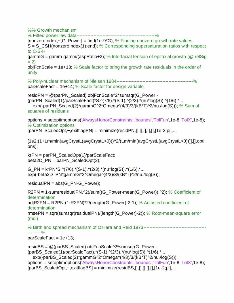
%% Growth mechanism
% Fitted power law data---------------------------------------------------%
[nonzeroIndex,~,G_Power] = find(1e-9*G); % Finding nonzero growth rate values
S = S_CSH(nonzeroIndex(1):end); % Corresponding supersaturation ratios with respect to C-S-H
gammG = gamm-gamm/(aspRatio+2); % Interfacial tension of epitaxial growth (@ relSig = 2)
objFcnScale = 1e+13; % Scale factor to bring the growth rate residuals in the order of unity
% Poly-nuclear mechanism of Nielsen 1984--------------------------------------------------%
parScaleFact = 1e+14; % Scale factor for design variable
residPN = @(parPN_Scaled) objFcnScale^2*sumsqr(G_Power - (parPN_Scaled(1)/parScaleFact)*S.^(7/6).*(S-1).^(2/3).*(nu*log(S)).^(1/6).*... exp(-parPN_Scaled(2)*gammG^2*Omega^(4/3)/3/(kB*T)^2/nu./log(S))); % Sum of squares of residuals
options = setoptimoptions('AlwaysHonorConstraints','bounds','TolFun',1e-8,'TolX',1e-8); % Optimization options
[parPN_ScaledOpt,~,exitflagPN] = minimize(residPN,[],[],[],[],[],[1e-2;pi],... [1e2;(1+Lm/min(avgCrystL(avgCrystL>0)))^2/(Lm/min(avgCrystL(avgCrystL>0)))],[],options); krPN = parPN_ScaledOpt(1)/parScaleFact; beta2D_PN = parPN_ScaledOpt(2); G_PN = krPN*S.^(7/6).*(S-1).^(2/3).*(nu*log(S)).^(1/6).*... exp(-beta2D_PN*gammG^2*Omega^(4/3)/3/(kB*T)^2/nu./log(S));
residualPN = abs(G_PN-G_Power); R2PN = 1-sum(residualPN.^2)/sum((G_Power-mean(G_Power)).^2); % Coefficient of determination
adjR2PN = R2PN-(1-R2PN)*2/(length(G_Power)-2-1); % Adjusted coefficient of determination
rmsePN = sqrt(sumsqr(residualPN)/(length(G_Power)-2)); % Root-mean-square error (mol)
% Birth and spread mechanism of O'Hara and Reid 1973--------------------------------------------------%
parScaleFact = 1e+13; residBS = @(parBS_Scaled) objFcnScale^2*sumsqr(G_Power - (parBS_Scaled(1)/parScaleFact).*(S-1).^(2/3).*(nu*log(S)).^(1/6).*... exp(-parBS_Scaled(2)*gammG^2*Omega^(4/3)/3/(kB*T)^2/nu./log(S))); options = setoptimoptions('AlwaysHonorConstraints','bounds','TolFun',1e-8,'TolX',1e-8); [parBS_ScaledOpt,~,exitflagBS] = minimize(residBS,[],[],[],[],[],[1e-2;pi],...
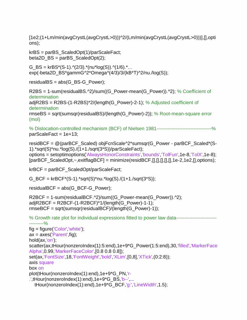
[1e2;(1+Lm/min(avgCrystL(avgCrystL>0)))^2/(Lm/min(avgCrystL(avgCrystL>0)))],[],options); krBS = parBS_ScaledOpt(1)/parScaleFact; beta2D_BS = parBS_ScaledOpt(2); G_BS = krBS*(S-1).^(2/3).*(nu*log(S)).^(1/6).*... exp(-beta2D_BS*gammG^2*Omega^(4/3)/3/(kB*T)^2/nu./log(S));
residualBS = abs(G_BS-G_Power); R2BS = 1-sum(residualBS.^2)/sum((G_Power-mean(G_Power)).^2); % Coefficient of determination
adjR2BS = R2BS-(1-R2BS)*2/(length(G_Power)-2-1); % Adjusted coefficient of determination
rmseBS = sqrt(sumsqr(residualBS)/(length(G_Power)-2)); % Root-mean-square error (mol)
% Dislocation-controlled mechanism (BCF) of Nielsen 1981----------------------------------%
parScaleFact = 1e+13; residBCF = @(parBCF_Scaled) objFcnScale^2*sumsqr(G_Power - parBCF_Scaled*(S-1).*sqrt(S)*nu.*log(S)./(1+1./sqrt(3*S))/parScaleFact); options = setoptimoptions('AlwaysHonorConstraints','bounds','TolFun',1e-8,'TolX',1e-8); [parBCF_ScaledOpt,~,exitflagBCF] = minimize(residBCF,[],[],[],[],[],1e-2,1e2,[],options); krBCF = parBCF_ScaledOpt/parScaleFact; G_BCF = krBCF*(S-1).*sqrt(S)*nu.*log(S)./(1+1./sqrt(3*S)); residualBCF = abs(G_BCF-G_Power); R2BCF = 1-sum(residualBCF.^2)/sum((G_Power-mean(G_Power)).^2); adjR2BCF = R2BCF-(1-R2BCF)*1/(length(G_Power)-1-1); rmseBCF = sqrt(sumsqr(residualBCF)/(length(G_Power)-1)); % Growth rate plot for individual expressions fitted to power law data----------------------------------%
fig = figure('Color','white'); ax = axes('Parent',fig); hold(ax,'on'); scatter(ax,tHour(nonzeroIndex(1):5:end),1e+9*G_Power(1:5:end),30,'filled','MarkerFaceAlpha',0.99,'MarkerFaceColor',[0.8 0.8 0.8]); set(ax,'FontSize',18,'FontWeight','bold','XLim',[0,8],'XTick',(0:2:8)); axis square
box on
plot(tHour(nonzeroIndex(1):end),1e+9*G_PN,'r-.',tHour(nonzeroIndex(1):end),1e+9*G_BS,'b--',... tHour(nonzeroIndex(1):end),1e+9*G_BCF,'g:','LineWidth',1.5);

scatter(ax,tHour(1:5:nonzeroIndex(1)-1),G(1:5:nonzeroIndex(1)-1),30,'filled','MarkerFaceAlpha',0.99,'MarkerFaceColor',[0.8 0.8 0.8])
xlabel('Time (h)','FontSize',18,'FontWeight','bold')
ylabel('Growth rate (nm/s)','FontSize',18,'FontWeight','bold')
legend({'Power law','Poly-nuclear (Nielsen 1984)','B&S (O`Hara and Reid 1973)','BCF (Nielsen 1981)'},'location','northeast','FontSize',18); % Compound B&S and BCF----------------------------------%
parScaleFact = 1e+13; residComp = @(parComp_Scaled) objFcnScale^2*sumsqr(G_Power - ... (parComp_Scaled(1)/parScaleFact)*(S-1).*sqrt(S)*nu.*log(S)./(1+1./sqrt(3*S)) - ... (parComp_Scaled(2)/parScaleFact)*(S-1).^(2/3).*(nu*log(S)).^(1/6).*... exp(-parComp_Scaled(3)*Omega^(4/3)*gammG^2/3/(kB*T)^2/nu./log(S)));
options = setoptimoptions('AlwaysHonorConstraints','bounds','TolFun',1e-12,'TolX',1e-12); [parComp_ScaledOpt,~,exitflagComp] = minimize(residComp,[],[],[],[],[],[1e-2;1e-2;pi],... [1e2;1e2;(1+Lm/min(avgCrystL(avgCrystL>0)))^2/(Lm/min(avgCrystL(avgCrystL>0)))],[],options); % Alternative optimization function (uncomment for use)
% [parCompOpt_scaled,~,exitflagComp] = fmincon(residComp,[1;1;1],[],[],[],[],[1e-2;1e-2],[1e2;1e2]); krBCF_Comp = parComp_ScaledOpt(1)/parScaleFact; krBS_Comp = parComp_ScaledOpt(2)/parScaleFact; beta2D_Comp = parComp_ScaledOpt(3); G_CompFcn = @(parComp_Scaled) (parComp_Scaled(1)/parScaleFact)*(S-1).*sqrt(S)*nu.*log(S)./(1+1./sqrt(3*S)) + ... (parComp_Scaled(2)/parScaleFact)*(S-1).^(2/3).*(nu*log(S)).^(1/6).*... exp(-parComp_Scaled(3)*Omega^(4/3)*gammG^2/3/(kB*T)^2/nu./log(S));
G_Comp = G_CompFcn(parComp_ScaledOpt); residualComp = abs(G_Comp-G_Power); R2Comp = 1-sum(residualComp.^2)/sum((G_Power-mean(G_Power)).^2); adjR2Comp = R2Comp-(1-R2Comp)*3/(length(G_Power)-3-1); rmseComp = sqrt(sumsqr(residualComp)/(length(G_Power)-3)); % Numerical Jacobian of compound growth rate function with respect to its input parameters
J = zeros(length(G_Power),length(parComp_ScaledOpt)); parfor j=1:length(parComp_ScaledOpt)
parComp_ScaledOptPlus = parComp_ScaledOpt; parComp_ScaledOptPlus(j) = parComp_ScaledOpt(j)+hStep; J(:,j) = (G_CompFcn(parComp_ScaledOptPlus)-G_Comp)/hStep; end

% Confidence intevals for compound growth rate parameters
pMatrixComp = inv(J'*J); % Precision matrix
covComp = sumsqr(residualComp)*pMatrixComp/(length(residualComp)-length(parComp_ScaledOpt)); % Covariance matrix
% Confidence interval half-width; parComp_ScaledOpt±ciHW_Comp
ciHW_Comp = tinv(0.95,length(residualComp)-length(parComp_ScaledOpt))*sqrt(diag(covComp))./[parScaleFact;parScaleFact;1]; %% Growth activation barriers and critical size of 2D nuclei hPlanck = 6.626069934e-34; % Planck constant (J.s)
% BCF activation barrier
EaBCF_LB = -log(hPlanck*krBCF_Comp*4*pi*Lm*gammG*exp(Lm^2*gammG/kB/T)/30/sqrt(KspSI)/solventOmega/NA/(kB*T)^2)*kB*T*NA/1000; EaBCF_UB = -log(hPlanck*krBCF_Comp*4*pi*Lm*gammG*exp(Lm^2*gammG/kB/T)/200/sqrt(KspSI)/solventOmega/NA/(kB*T)^2)*kB*T*NA/1000; % B&S activation barrier
EaBS_LB = -log(hPlanck*krBS_Comp/2/Lm/(30*sqrt(KspSI)/rhoMolar)^(4/3)/exp(-gammG*Lm^2/kB/T)/kB/T)*kB*T*NA/1000; EaBS_UB = -log(hPlanck*krBS_Comp/2/Lm/(200*sqrt(KspSI)/rhoMolar)^(4/3)/exp(-gammG*Lm^2/kB/T)/kB/T)*kB*T*NA/1000; G_Comp_BCF = krBCF_Comp*(S-1).*sqrt(S)*nu.*log(S)./(1+1./sqrt(3*S)); % BCF part of growth rate
G_Comp_BS = krBS_Comp*(S-1).^(2/3).*(nu*log(S)).^(1/6).*... exp(-beta2D_Comp*Omega^(4/3)*gammG^2/3/(kB*T)^2/nu./log(S)); % B&S part of growth rate
% Activation free energy for surface nucleation
[row,~,~] = find(G_Comp_BS(G_Comp_BS>1e-16)); EaSurfNucl_LB = min(1e-3*NA*beta2D_Comp*Omega^(4/3)*gammG^2/(kB*T)/nu./log(S)); EaSurfNucl_UB = 1e-3*NA*beta2D_Comp*Omega^(4/3)*gammG^2/(kB*T)/nu./log(S(max(row)));
% Critical size of surface nuclei L2D = 1e9*2*gammG*Lm^3/kB/T/nu./log(S); % Cylindrical surface nuclei (nm)
% Plot of BCF and B&S components of growth rate along with critical size of
% surface nuclei fig = figure('Color','white'); [ax,hLine1,hLine2] = plotyy([tHour(nonzeroIndex(1):end),tHour(nonzeroIndex(1):end),tHour(nonzeroIndex(1):end)],... 1e9*[G_Comp_BS,G_Comp_BCF,G_Comp],tHour(nonzeroIndex(1):end),L2D); set(fig,'CurrentAxes',ax)
xlabel('Time (h)','FontSize',18,'FontWeight','bold')

ylabel(ax(1),'Growth rate (nm/s)','FontSize',18,'FontWeight','bold') % left y-axis
ylabel(ax(2),'Size of critical surface nuclei (nm)','FontSize',18,'FontWeight','bold','Color',[0.6 0.6 0.6]) % right y-axis
set(hLine1(1),'Color','b','LineStyle','--','LineWidth',1.5); set(hLine1(2),'Color','g','LineStyle',':','LineWidth',1.5); set(hLine1(3),'Color','k','LineStyle','-','LineWidth',1.5); set(hLine2,'Color','r','LineStyle','-.','LineWidth',1); set(ax,'FontSize',18,'FontWeight','bold','XLim',[floor(tHour(nonzeroIndex(1))*10)/10,5],'PlotBoxAspectRatio',[1 1 1]); set(ax(1),'YTick',linspace(0,ceil(max(1e13*G_Comp))*1e-4,6),'YLim',[0,ceil(max(1e13*G_Comp))*1e-4],'YColor','k'); set(ax(2),'YTick',linspace(0,floor(1e9*avgCrystL(end)*aspRatio*10)/10,6),'YLim',[0,floor(1e9*avgCrystL(end)*aspRatio*10)/10],'YColor','r'); legend({'B&S','BCF','Compound B&S+BCF'},'FontSize',18,'Location','north'); fig = figure('Color','white'); [ax,hLine1,hLine2] = plotyy([tHour(nonzeroIndex(1):end),tHour(nonzeroIndex(1):end)],... 1e9*[G_Comp_BS,G_Comp_BCF],tHour(nonzeroIndex(1):end),G_Comp_BCF./G_Comp_BS); set(fig,'CurrentAxes',ax)
xlabel('Time (h)','FontSize',18,'FontWeight','bold')
ylabel(ax(1),'Growth rate (nm/s)','FontSize',18,'FontWeight','bold') % left y-axis
ylabel(ax(2),'G_{BCF}/G_{B&S}','FontSize',18,'FontWeight','bold','Color',[0.6 0.6 0.6]) % right y-axis
set(hLine1(1),'Color','b','LineStyle','--','LineWidth',1.5); set(hLine1(2),'Color','g','LineStyle',':','LineWidth',1.5); set(hLine2,'Color','r','LineStyle','-.','LineWidth',1); set(ax,'FontSize',18,'FontWeight','bold','XLim',[floor(tHour(nonzeroIndex(1))*10)/10,5],'PlotBoxAspectRatio',[1 1 1]); set(ax(1),'YTick',linspace(0,ceil(max(1e13*G_Comp_BCF))*1e-4,6),'YLim',[0,ceil(max(1e13*G_Comp_BCF))*1e-4],'YColor','k'); set(ax(2),'YTick',linspace(0,6,6),'YLim',[0,6],'YColor','r'); legend({'B&S','BCF','Compound B&S+BCF'},'FontSize',18,'Location','north'); %% Plots of nucleation rates and barriers, growth rate, supersaturation, sizes, and contributions
fig = figure('Color','white'); subplot(1,2,1)
[ax,hLine1,hLine2] = plotyy([tHour,tHour],[log10(JI),log10(JII)],[tHour,tHour],[LI,LII]); set(fig,'CurrentAxes',ax)
xlabel('Time (h)','FontSize',18,'FontWeight','bold')
ylabel(ax(1),'log_{10}(nucleation rate/s^{-1})','FontSize',18,'FontWeight','bold') % left y-axis
ylabel(ax(2),'Thickness of critical nuclei (nm)','FontSize',18,'FontWeight','bold','Color',[0.6 0.6 0.6]) % right y-axis
set(hLine1(1),'Color','b','LineWidth',1.5);

set(hLine1(2),'Color','b','LineStyle','--','LineWidth',1.5); set(hLine2(1),'Color','r','LineWidth',1.5); set(hLine2(2),'Color','r','LineStyle','--','LineWidth',1.5); set(ax,'FontSize',18,'FontWeight','bold','XLim',[0,2.5],'PlotBoxAspectRatio',[1 1 1]); set(ax(1),'YTick',linspace(0,20,6),'YLim',[0,20],'YColor','b'); set(ax(2),'YTick',linspace(0,4,6),'YLim',[0,4],'YColor','r'); legend({'Primary nucleation','Secondary nucleation'},'FontSize',18,'Location','north'); ax = subplot(1,2,2); hold(ax,'on'); plot(tHour,EaJI,'r',tHour,EaJII,'b--','LineWidth',1.5); set(ax,'FontSize',18,'FontWeight','bold','XLim',[0,2.5],'YLim',[0,300]); axis square
box on
xlabel('Time (h)','FontSize',18,'FontWeight','bold')
ylabel('\DeltaG_{max} (kJ/mol)','FontSize',18,'FontWeight','bold')
legend({'Primary nucleation','Secondary nucleation'},'FontSize',18,'Location','south'); figure('Color','white'); ax = subplot(1,2,1); hold(ax,'on'); scatter(ax,[tHour(1:5:nonzeroIndex(1)-1);tHour(nonzeroIndex(1):5:end)],1e+9*[G(1:5:nonzeroIndex(1)-1);G_Power(1:5:end)],... 30,'filled','MarkerFaceAlpha',0.9,'MarkerFaceColor',[0.8 0.8 0.8]); set(ax,'FontSize',18,'FontWeight','bold','XLim',[0,8],'XTick',(0:2:8)); axis square
box on
plot(tHour(nonzeroIndex(1):end),1e+9*G_BS,'b--',... tHour(nonzeroIndex(1):end),1e+9*G_BCF,'g:',... tHour(nonzeroIndex(1):end),1e+9*G_Comp,'k-','LineWidth',1); xlabel('Time (h)','FontSize',18,'FontWeight','bold')
ylabel('Growth rate (nm/s)','FontSize',18,'FontWeight','bold')
legend({'Power law','B&S','BCF','BCF+B&S'},'location','northeast','FontSize',18); ax = subplot(1,2,2); hold(ax,'on'); plot(tHour,S_CSH,'b',tHour,S_Port,'r--',[0,24],[1,1],'k:','LineWidth',1.5); set(ax,'FontSize',18,'FontWeight','bold','Xlim',[0,24],'XTick',(0:4:24)); axis square
box on
xlabel('Time (h)','FontSize',18,'FontWeight','bold')
ylabel('Supersaturation ratio','FontSize',18,'FontWeight','bold')
legend({'C-S-H','Portlandite'},'FontSize',18); fig = figure('Color','white'); ax = subplot(1,2,1); hold(ax,'on'); [ax,hLine1,hLine2] = plotyy(tHour,1e+9*avgCrystL,tHour,1e+9*avgPartL);
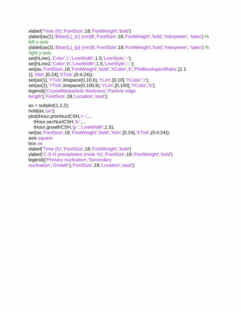
xlabel('Time (h)','FontSize',18,'FontWeight','bold')
ylabel(ax(1),'$\bar{L}_{c} (nm)$','FontSize',18,'FontWeight','bold','Interpreter', 'latex') % left y-axis
ylabel(ax(2),'$\bar{L}_{p} (nm)$','FontSize',18,'FontWeight','bold','Interpreter', 'latex') % right y-axis
set(hLine1,'Color','r','LineWidth',1.5,'LineStyle','-'); set(hLine2,'Color','b','LineWidth',1.5,'LineStyle','--'); set(ax,'FontSize',18,'FontWeight','bold','XColor','k','PlotBoxAspectRatio',[1 1 1],'Xlim',[0,24],'XTick',(0:4:24)); set(ax(1),'YTick',linspace(0,10,6),'YLim',[0,10],'YColor','r'); set(ax(2),'YTick',linspace(0,100,6),'YLim',[0,100],'YColor','b'); legend({'Crystallite/particle thickness','Particle edge length'},'FontSize',18,'Location','east'); ax = subplot(1,2,2); hold(ax,'on'); plot(tHour,primNuclCSH,'r--',... tHour,secNuclCSH,'b:',... tHour,growthCSH,'g-.','LineWidth',1.5); set(ax,'FontSize',18,'FontWeight','bold','Xlim',[0,24],'XTick',(0:4:24)); axis square
box on
xlabel('Time (h)','FontSize',18,'FontWeight','bold')
ylabel('C-S-H precipitated (mole %)','FontSize',18,'FontWeight','bold')
legend({'Primary nucleation','Secondary nucleation','Growth'},'FontSize',18,'Location','east');
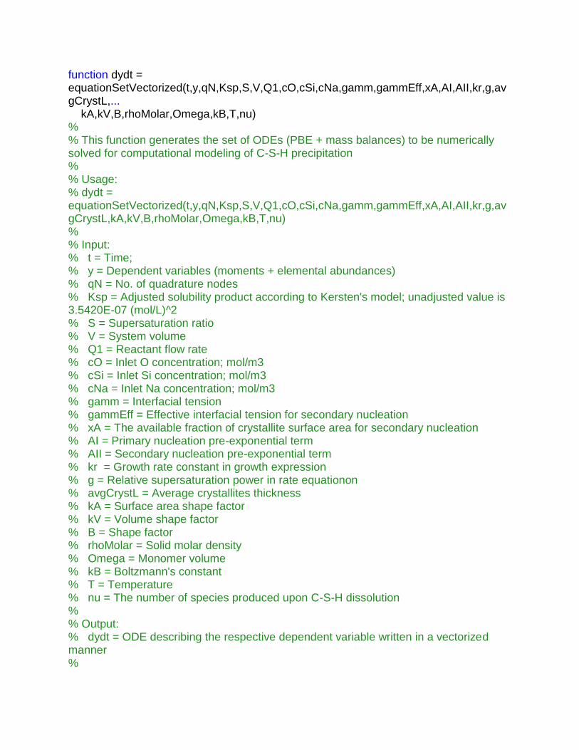
function dydt = equationSetVectorized(t,y,qN,Ksp,S,V,Q1,cO,cSi,cNa,gamm,gammEff,xA,AI,AII,kr,g,avgCrystL,... kA,kV,B,rhoMolar,Omega,kB,T,nu)
% % This function generates the set of ODEs (PBE + mass balances) to be numerically solved for computational modeling of C-S-H precipitation % % Usage: % dydt = equationSetVectorized(t,y,qN,Ksp,S,V,Q1,cO,cSi,cNa,gamm,gammEff,xA,AI,AII,kr,g,avgCrystL,kA,kV,B,rhoMolar,Omega,kB,T,nu) % % Input: % t = Time; % y = Dependent variables (moments + elemental abundances)
% qN = No. of quadrature nodes
% Ksp = Adjusted solubility product according to Kersten's model; unadjusted value is 3.5420E-07 (mol/L)^2
% S = Supersaturation ratio
% V = System volume
% Q1 = Reactant flow rate
% cO = Inlet O concentration; mol/m3
% cSi = Inlet Si concentration; mol/m3
% cNa = Inlet Na concentration; mol/m3
% gamm = Interfacial tension
% gammEff = Effective interfacial tension for secondary nucleation
% xA = The available fraction of crystallite surface area for secondary nucleation
% AI = Primary nucleation pre-exponential term
% AII = Secondary nucleation pre-exponential term
% kr = Growth rate constant in growth expression
% g = Relative supersaturation power in rate equationon
% avgCrystL = Average crystallites thickness
% kA = Surface area shape factor
% kV = Volume shape factor
% B = Shape factor
% rhoMolar = Solid molar density
% Omega = Monomer volume
% kB = Boltzmann's constant % T = Temperature
% nu = The number of species produced upon C-S-H dissolution
% % Output: % dydt = ODE describing the respective dependent variable written in a vectorized manner
%

% This function is part of the MATLAB workflow on "population balance modeling of calcium-silicate-hydrate precipitaion" developed by M. Reza Andalibi at Paul Scherrer Institute/EPFL (2017). % Please cite our article: % M. Reza Andalibi et al., "On The Mesoscale Mechanism of Calcium-Silicate-Hydrate Precipitation: A Population Balance Modeling Approach", 2017. %% Initialization
yNo = size(y,2); % Number of y vectors
dydt = zeros(4+2*qN,yNo); % Initialization
%% Unit correction for Ksp from (mol/L)^nu to SI unit KspSI = Ksp*1000^nu; % Solubility product in SI units (mol/m3)^nu
%% Discretized growth expression in PBE
Li = zeros(qN,yNo); % Quadrature nodes
wi = zeros(qN,yNo); % Quadrature weights
for j=1:yNo
[Li(:,j),wi(:,j)] = WH(y(1:2*qN,j),qN); % NDF construction from moments by Wheeler algorithm
end
if avgCrystL>0 % At least 1 crystallite has formed
Gi = kA*kr*KspSI^(g/nu)*(S-1)^g/(3*kV*rhoMolar); else
Gi = 0; end
%% ODEs for moments
if S<=1 % Zero nucleation rate for (under-)saturated solutions
JI = zeros(1,yNo); JII = zeros(1,yNo); LI = ones(1,yNo); LII = ones(1,yNo); else
LI = ( 2*kA*Omega*gamm/3/kV/kB/T/nu/log(S) )*ones(1,yNo); % m
JI = ( AI*(nu*log(S))^2*exp(-B*gamm^3*Omega^2/kB^3/T^3/nu^2/log(S)^2) )*ones(1,yNo); % #/(m3*s)
% Primary nucleation
A = kA*y(3,:); % Total crystallite surface area
LII = ( 2*kA*Omega*gammEff/3/kV/kB/T/nu/log(S) )*ones(1,yNo); % m
JII = AII*(nu*log(S))^2*xA*A*exp(-B*gammEff^3*Omega^2/kB^3/T^3/nu^2/log(S)^2); % #/(m3*s)
% True secondary nucleation
end
for i=1:2*qN
k = i-1; % Moment order (0,...,2qN-1)
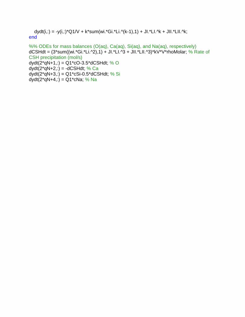
dydt(i,:) = -y(i,:)*Q1/V + k*sum(wi.*Gi.*Li.^(k-1),1) + JI.*LI.^k + JII.*LII.^k; end
%% ODEs for mass balances (O(aq), Ca(aq), Si(aq), and Na(aq), respectively)
dCSHdt = (3*sum((wi.*Gi.*Li.^2),1) + JI.*LI.^3 + JII.*LII.^3)*kV*V*rhoMolar; % Rate of CSH precipitation (mol/s)
dydt(2*qN+1,:) = Q1*cO-3.5*dCSHdt; % O
dydt(2*qN+2,:) = -dCSHdt; % Ca
dydt(2*qN+3,:) = Q1*cSi-0.5*dCSHdt; % Si dydt(2*qN+4,:) = Q1*cNa; % Na
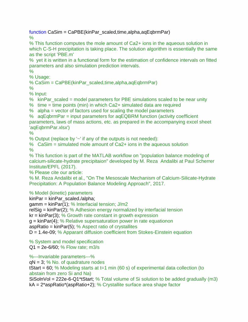
function CaSim = CaPBE(kinPar_scaled,time,alpha,aqEqbrmPar)
% % This function computes the mole amount of Ca2+ ions in the aqueous solution in which C-S-H precipitation is taking place. The solution algorithm is essentially the same as the script 'PBE.m' % yet it is written in a functional form for the estimation of confidence intervals on fitted parameters and also simulation prediction intervals.
% % Usage: % CaSim = CaPBE(kinPar_scaled,time,alpha,aqEqbrmPar)
% % Input: % kinPar_scaled = model parameters for PBE simulations scaled to be near unity
% time = time points (min) in which Ca2+ simulated data are required
% alpha = vector of factors used for scaling the model parameters
% aqEqbrmPar = input parameters for aqEQBRM function (activity coefficient parameters, laws of mass actions, etc. as prepared in the accompanying excel sheet 'aqEqbrmPar.xlsx')
% % Output (replace by '~' if any of the outputs is not needed): % CaSim = simulated mole amount of Ca2+ ions in the aqueous solution
% % This function is part of the MATLAB workflow on "population balance modeling of calcium-silicate-hydrate precipitaion" developed by M. Reza Andalibi at Paul Scherrer Institute/EPFL (2017). % Please cite our article: % M. Reza Andalibi et al., "On The Mesoscale Mechanism of Calcium-Silicate-Hydrate Precipitation: A Population Balance Modeling Approach", 2017. % Model (kinetic) parameters
kinPar = kinPar_scaled./alpha; gamm = kinPar(1); % Interfacial tension; J/m2
relSig = kinPar(2); % Adhesion energy normalized by interfacial tension
kr = kinPar(3); % Growth rate constant in growth expression
g = kinPar(4); % Relative supersaturation power in rate equationon
aspRatio = kinPar(5); % Aspect ratio of crystallites
D = 1.4e-09; % Apparant diffusion coefficient from Stokes-Einstein equation
% System and model specification
Q1 = 2e-6/60; % Flow rate; m3/s
%---Invariable parameters---%
qN = 3; % No. of quadrature nodes
tStart = 60; % Modeling starts at t=1 min (60 s) of experimental data collection (to abstain from zero Si and Na)
SiSolnVol = 222e-6-Q1*tStart; % Total volume of Si solution to be added gradually (m3)
kA = 2*aspRatio*(aspRatio+2); % Crystallite surface area shape factor
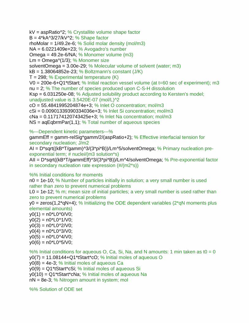
kV = aspRatio^2; % Crystallite volume shape factor
B = 4*kA^3/27/kV^2; % Shape factor
rhoMolar = 1/49.2e-6; % Solid molar density (mol/m3)
NA = 6.0221409e+23; % Avogadro's number
Omega = 49.2e-6/NA; % Monomer volume (m3)
Lm = Omega^(1/3); % Monomer size
solventOmega = 3.00e-29; % Molecular volume of solvent (water; m3)
kB = 1.38064852e-23; % Boltzmann's constant (J/K)
T = 298; % Experimental temperature (K)
V0 = 200e-6+Q1*tStart; % Initial reaction vessel volume (at t=60 sec of experiment); m3
nu = 2; % The number of species produced upon C-S-H dissolution
Ksp = 6.031250e-08; % Adjusted solubility product according to Kersten's model; unadjusted value is 3.5420E-07 (mol/L)^2
cO = 55.4841995204874e+3; % Inlet O concentration; mol/m3
cSi = 0.00901339390334036e+3; % Inlet Si concentration; mol/m3
cNa = 0.117174120743425e+3; % Inlet Na concentration; mol/m3
NS = aqEqbrmPar(1,1); % Total number of aqueous species
%---Dependent kinetic parameters---%
gammEff = gamm-relSig*gamm/2/(aspRatio+2); % Effective interfacial tension for secondary nucleation; J/m2
AI = D*sqrt((kB*T/gamm)^3/(3*pi*B))/Lm^5/solventOmega; % Primary nucleation pre-exponential term; # nuclei/(m3 solution*s)
AII = D*sqrt((kB*T/gammEff)^3/(3*pi*B))/Lm^4/solventOmega; % Pre-exponential factor in secondary nucleation rate expression (#/(m2*s))
%% Initial conditions for moments
n0 = 1e-10; % Number of particles initially in solution; a very small number is used rather than zero to prevent numerical problems
L0 = 1e-12; % m; mean size of initial particles; a very small number is used rather than zero to prevent numerical problems
y0 = zeros(1,2*qN+4); % Initializing the ODE dependent variables (2*qN moments plus elemental amounts)
y0(1) = n0*L0^0/V0; y0(2) = n0*L0^1/V0; y0(3) = n0*L0^2/V0; y0(4) = n0*L0^3/V0; y0(5) = n0*L0^4/V0; y0(6) = n0*L0^5/V0; %% Initial conditions for aqueous O, Ca, Si, Na, and N amounts: 1 min taken as t0 = 0
y0(7) = 11.08144+Q1*tStart*cO; % Initial moles of aqueous O
y0(8) = 4e-3; % Initial moles of aqueous Ca
y0(9) = Q1*tStart*cSi; % Initial moles of aqueous Si y0(10) = Q1*tStart*cNa; % Initial moles of aqueous Na
nN = 8e-3; % Nitrogen amount in system; mol %% Solution of ODE set
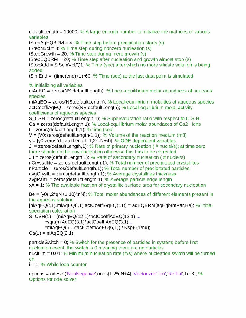
defaultLength = 10000; % A large enough number to initialize the matrices of various variables
tStepAqEQBRM = 4; % Time step before precipitation starts (s)
tStepNucl = 8; % Time step during nonzero nucleation (s)
tStepGrowth = 20; % Time step during mere growth (s)
tStepEQBRM = 20; % Time step after nucleation and growth almost stop (s)
tStopAdd = SiSolnVol/Q1; % Time (sec) after which no more silicate solution is being added
tSimEnd = (time(end)+1)*60; % Time (sec) at the last data point is simulated
% Initializing all variables
niAqEQ = zeros(NS,defaultLength); % Local-equilibrium molar abundaces of aqueous species
miAqEQ = zeros(NS,defaultLength); % Local-equilibrium molalities of aqueous species
actCoeffiAqEQ = zeros(NS,defaultLength); % Local-equilibrium molal activity coefficients of aqueous species
S_CSH = zeros(defaultLength,1); % Supersaturation ratio with respect to C-S-H
Ca = zeros(defaultLength,1); % Local-equilibrium molar abundaces of Ca2+ ions
t = zeros(defaultLength,1); % time (sec)
V = [V0;zeros(defaultLength-1,1)]; % Volume of the reaction medium (m3)
y = [y0;zeros(defaultLength-1,2*qN+4)]; % ODE dependent variables
JI = zeros(defaultLength,1); % Rate of primary nucleation ( # nuclei/s); at time zero there should not be any nucleation otherwise this has to be corrected
JII = zeros(defaultLength,1); % Rate of secondary nucleation ( # nuclei/s)
nCrystallite = zeros(defaultLength,1); % Total number of precipitated crystallites
nParticle = zeros(defaultLength,1); % Total number of precipitated particles
avgCrystL = zeros(defaultLength,1); % Average crystallites thickness
avgPartL = zeros(defaultLength,1); % Average particle edge length
xA = 1; % The available fraction of crystallite surface area for secondary nucleation
Be = [y0(:,2*qN+1:10)';nN]; % Total molar abundances of different elements present in the aqueous solution
[niAqEQ(:,1),miAqEQ(:,1),actCoeffiAqEQ(:,1)] = aqEQBRM(aqEqbrmPar,Be); % Initial speciation calculation
S_CSH(1) = (miAqEQ(12,1)*actCoeffiAqEQ(12,1) ... *sqrt(miAqEQ(3,1)*actCoeffiAqEQ(3,1)... *miAqEQ(6,1)*actCoeffiAqEQ(6,1)) / Ksp)^(1/nu); Ca(1) = niAqEQ(2,1); particleSwitch = 0; % Switch for the presence of particles in system; before first nucleation event, the switch is 0 meaning there are no particles
nuclLim = 0.01; % Minimum nucleation rate (#/s) where nucleation switch will be turned on
i = 1; % While loop counter
options = odeset('NonNegative',ones(1,2*qN+4),'Vectorized','on','RelTol',1e-8); % Options for ode solver
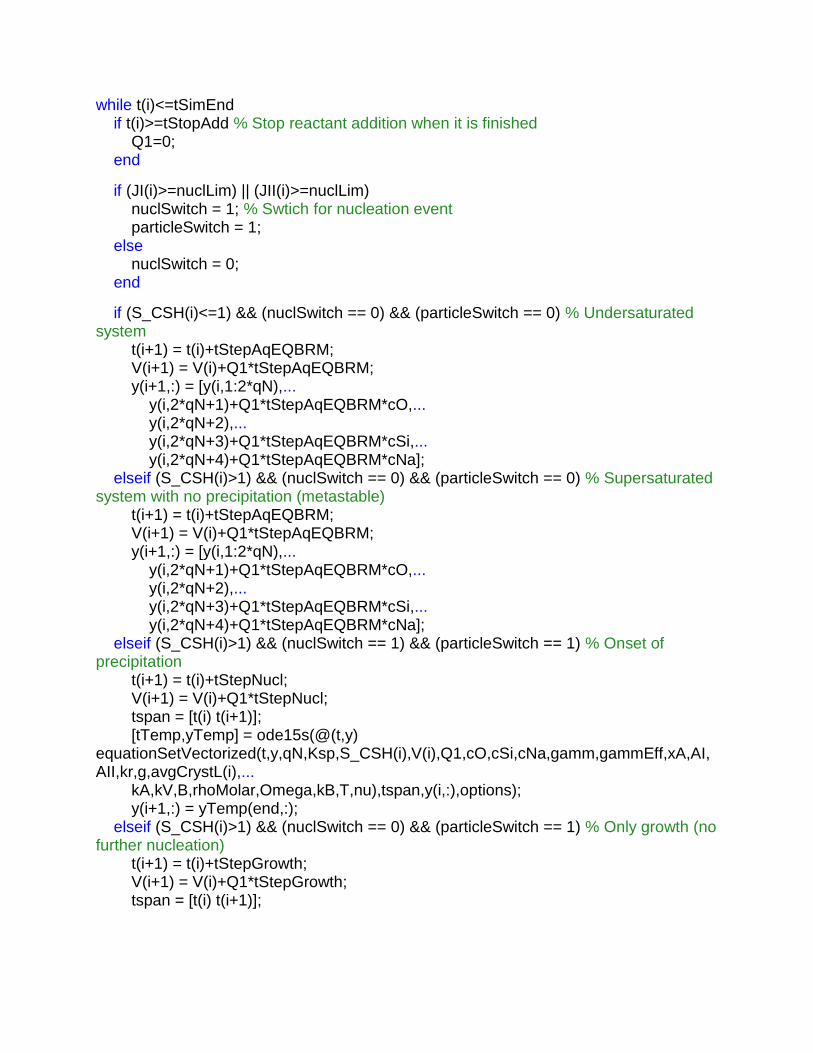
while t(i)<=tSimEnd
if t(i)>=tStopAdd % Stop reactant addition when it is finished
Q1=0; end
if (JI(i)>=nuclLim) || (JII(i)>=nuclLim)
nuclSwitch = 1; % Swtich for nucleation event particleSwitch = 1; else
nuclSwitch = 0; end
if (S_CSH(i)<=1) && (nuclSwitch == 0) && (particleSwitch == 0) % Undersaturated system
t(i+1) = t(i)+tStepAqEQBRM; V(i+1) = V(i)+Q1*tStepAqEQBRM; y(i+1,:) = [y(i,1:2*qN),... y(i,2*qN+1)+Q1*tStepAqEQBRM*cO,... y(i,2*qN+2),... y(i,2*qN+3)+Q1*tStepAqEQBRM*cSi,... y(i,2*qN+4)+Q1*tStepAqEQBRM*cNa]; elseif (S_CSH(i)>1) && (nuclSwitch == 0) && (particleSwitch == 0) % Supersaturated system with no precipitation (metastable)
t(i+1) = t(i)+tStepAqEQBRM; V(i+1) = V(i)+Q1*tStepAqEQBRM; y(i+1,:) = [y(i,1:2*qN),... y(i,2*qN+1)+Q1*tStepAqEQBRM*cO,... y(i,2*qN+2),... y(i,2*qN+3)+Q1*tStepAqEQBRM*cSi,... y(i,2*qN+4)+Q1*tStepAqEQBRM*cNa]; elseif (S_CSH(i)>1) && (nuclSwitch == 1) && (particleSwitch == 1) % Onset of precipitation
t(i+1) = t(i)+tStepNucl; V(i+1) = V(i)+Q1*tStepNucl; tspan = [t(i) t(i+1)]; [tTemp,yTemp] = ode15s(@(t,y) equationSetVectorized(t,y,qN,Ksp,S_CSH(i),V(i),Q1,cO,cSi,cNa,gamm,gammEff,xA,AI,AII,kr,g,avgCrystL(i),... kA,kV,B,rhoMolar,Omega,kB,T,nu),tspan,y(i,:),options); y(i+1,:) = yTemp(end,:); elseif (S_CSH(i)>1) && (nuclSwitch == 0) && (particleSwitch == 1) % Only growth (no further nucleation)
t(i+1) = t(i)+tStepGrowth; V(i+1) = V(i)+Q1*tStepGrowth; tspan = [t(i) t(i+1)];
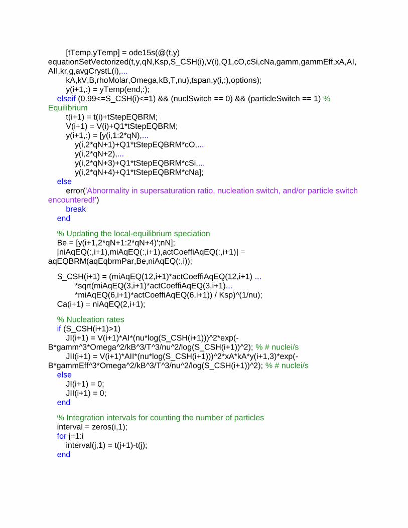
[tTemp,yTemp] = ode15s(@(t,y) equationSetVectorized(t,y,qN,Ksp,S_CSH(i),V(i),Q1,cO,cSi,cNa,gamm,gammEff,xA,AI,AII,kr,g,avgCrystL(i),... kA,kV,B,rhoMolar,Omega,kB,T,nu),tspan,y(i,:),options); y(i+1,:) = yTemp(end,:); elseif (0.99<=S_CSH(i)<=1) && (nuclSwitch == 0) && (particleSwitch == 1) % Equilibrium
t(i+1) = t(i)+tStepEQBRM; V(i+1) = V(i)+Q1*tStepEQBRM; y(i+1,:) = [y(i,1:2*qN),... y(i,2*qN+1)+Q1*tStepEQBRM*cO,... y(i,2*qN+2),... y(i,2*qN+3)+Q1*tStepEQBRM*cSi,... y(i,2*qN+4)+Q1*tStepEQBRM*cNa]; else
error('Abnormality in supersaturation ratio, nucleation switch, and/or particle switch encountered!')
break
end
% Updating the local-equilibrium speciation
Be = [y(i+1,2*qN+1:2*qN+4)';nN]; [niAqEQ(:,i+1),miAqEQ(:,i+1),actCoeffiAqEQ(:,i+1)] = aqEQBRM(aqEqbrmPar,Be,niAqEQ(:,i)); S_CSH(i+1) = (miAqEQ(12,i+1)*actCoeffiAqEQ(12,i+1) ... *sqrt(miAqEQ(3,i+1)*actCoeffiAqEQ(3,i+1)... *miAqEQ(6,i+1)*actCoeffiAqEQ(6,i+1)) / Ksp)^(1/nu); Ca(i+1) = niAqEQ(2,i+1); % Nucleation rates
if (S_CSH(i+1)>1)
JI(i+1) = V(i+1)*AI*(nu*log(S_CSH(i+1)))^2*exp(-B*gamm^3*Omega^2/kB^3/T^3/nu^2/log(S_CSH(i+1))^2); % # nuclei/s
JII(i+1) = V(i+1)*AII*(nu*log(S_CSH(i+1)))^2*xA*kA*y(i+1,3)*exp(-B*gammEff^3*Omega^2/kB^3/T^3/nu^2/log(S_CSH(i+1))^2); % # nuclei/s
else
JI(i+1) = 0; JII(i+1) = 0; end
% Integration intervals for counting the number of particles
interval = zeros(i,1); for j=1:i interval(j,1) = t(j+1)-t(j); end
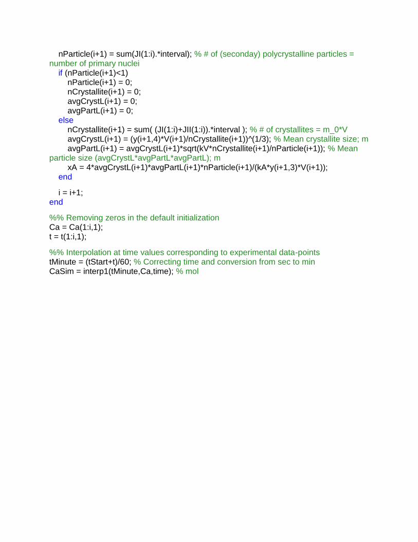
nParticle(i+1) = sum(JI(1:i).*interval); % # of (seconday) polycrystalline particles = number of primary nuclei if (nParticle(i+1)<1)
nParticle(i+1) = 0; nCrystallite(i+1) = 0; avgCrystL(i+1) = 0; avgPartL(i+1) = 0; else
nCrystallite(i+1) = sum( (JI(1:i)+JII(1:i)).*interval ); % # of crystallites = m_0*V
avgCrystL(i+1) = (y(i+1,4)*V(i+1)/nCrystallite(i+1))^(1/3); % Mean crystallite size; m
avgPartL(i+1) = avgCrystL(i+1)*sqrt(kV*nCrystallite(i+1)/nParticle(i+1)); % Mean particle size (avgCrystL*avgPartL*avgPartL); m
xA = 4*avgCrystL(i+1)*avgPartL(i+1)*nParticle(i+1)/(kA*y(i+1,3)*V(i+1));
end
i = i+1; end
%% Removing zeros in the default initialization
Ca = Ca(1:i,1); t = t(1:i,1); %% Interpolation at time values corresponding to experimental data-points
tMinute = (tStart+t)/60; % Correcting time and conversion from sec to min
CaSim = interp1(tMinute,Ca,time); % mol

function [Li,w]=WH(m,N)
% This code was taken from the Appendix A.1.2 of the following reference: % Marchisio, D. L., & Fox, R. O. (2013). Computational models for polydisperse particulate and multiphase systems. Cambridge University Press.
% compute quadrature approximation with the Wheeler algorithm
%
% INPUT: % N = number of nodes of the quadrature approximation
% m = moments from 0 to 2N-1 [mom(1), ..., mom(2N)] %
% OUTPUT: % Li = abscissas
% w = weights
%
% compute intermediate coefficients
%
for l=1:2*N-2
sigma(1,l+1) = 0.0; end
%
for l=0:2*N-1
sigma(2,l+1) = m(l+1); end
%
% compute coefficients for Jacobi matrix
%
a(1) = m(2)/m(1); b(1) = 0.0; %
for k=1:N-1
for l=k:2*N-k-1
sigma(k+2,l+1) = sigma(k+1,l+2)-a(k)*sigma(k+1,l+1)-b(k)*sigma(k,l+1); a(k+1) = -sigma(k+1,k+1)/sigma(k+1,k)+sigma(k+2,k+2)/sigma(k+2,k+1); b(k+1) = sigma(k+2,k+1)/sigma(k+1,k); end
end
% compute Jacobi matrix
%
for i=1:N
jacobi(i,i)=a(i); end
%
for i=1:N-1
jacobi(i,i+1) = -(abs(b(i+1)))^0.5; jacobi(i+1,i) = -(abs(b(i+1)))^0.5; end
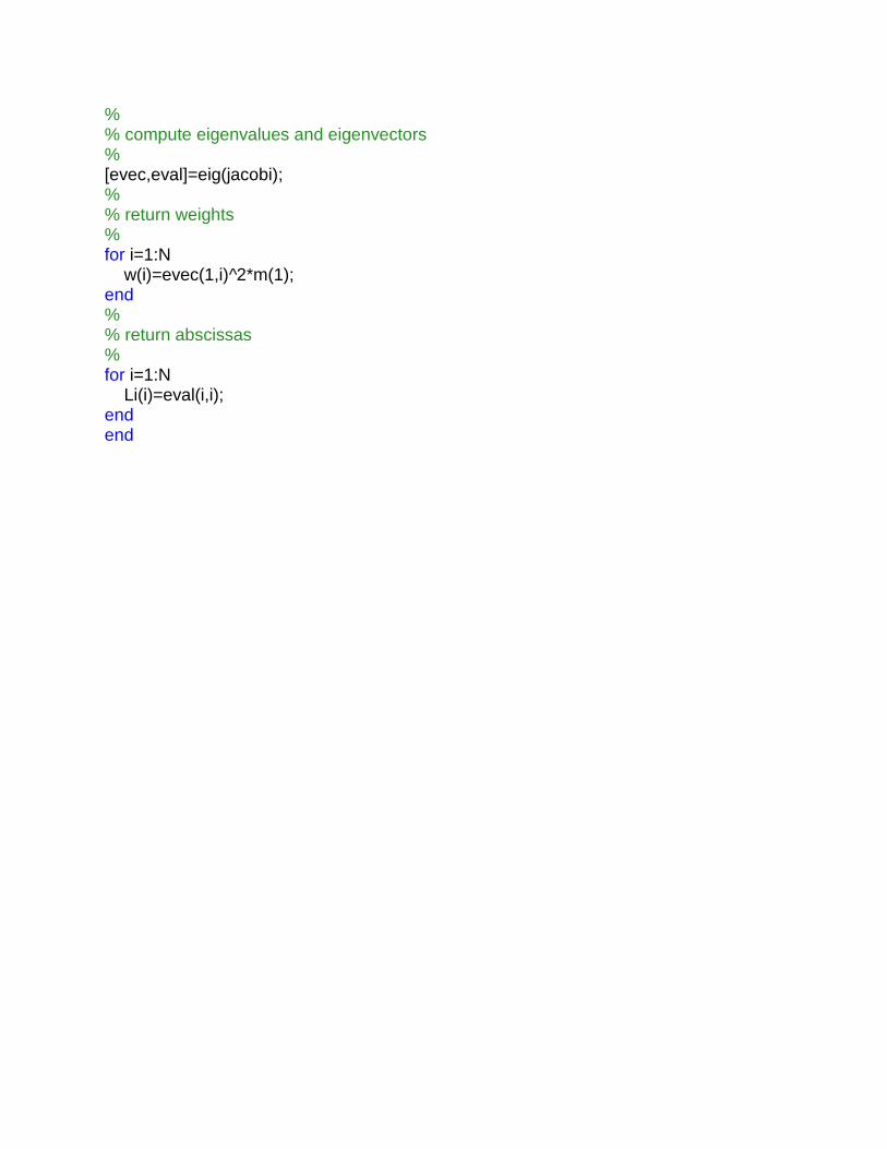
%
% compute eigenvalues and eigenvectors
%
[evec,eval]=eig(jacobi); %
% return weights
%
for i=1:N
w(i)=evec(1,i)^2*m(1); end
%
% return abscissas
%
for i=1:N
Li(i)=eval(i,i); end
end