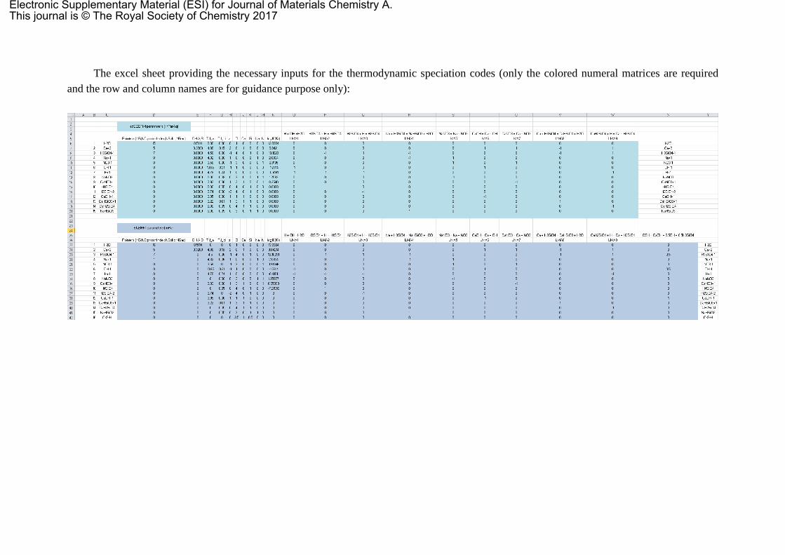
The excel sheet providing the necessary inputs for the thermodynamic speciation codes (only the colored numeral matrices are required
and the row and column names are for guidance purpose only):
Electronic Supplementary Material (ESI) for Journal of Materials Chemistry A.This journal is © The Royal Society of Chemistry 2017
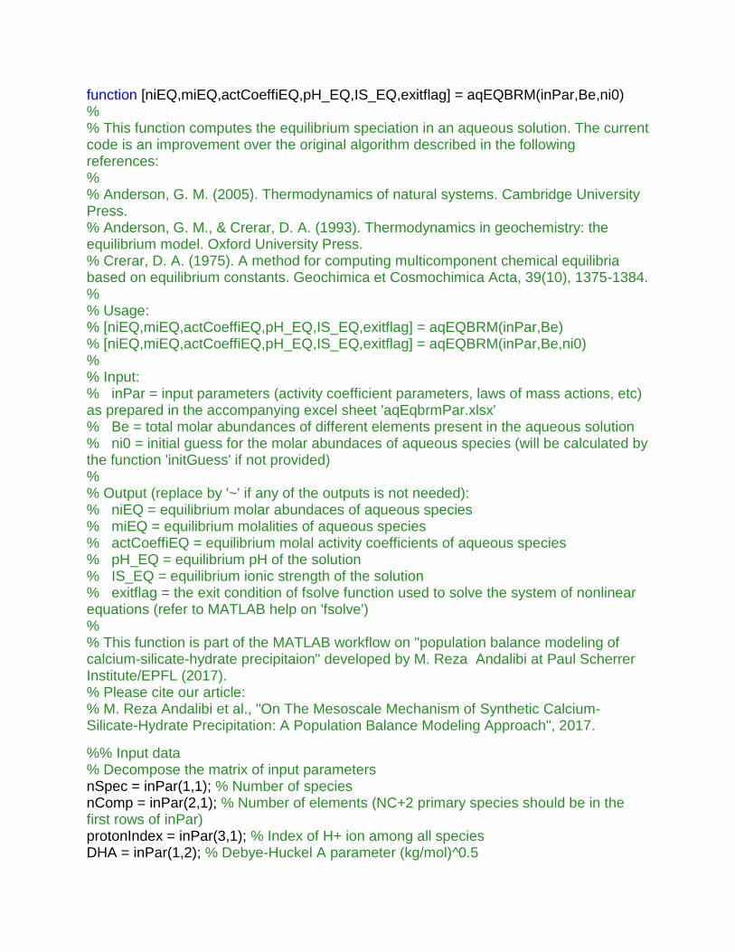
function [niEQ,miEQ,actCoeffiEQ,pH_EQ,IS_EQ,exitflag] = aqEQBRM(inPar,Be,ni0)
% % This function computes the equilibrium speciation in an aqueous solution. The current code is an improvement over the original algorithm described in the following references: % % Anderson, G. M. (2005). Thermodynamics of natural systems. Cambridge University Press. % Anderson, G. M., & Crerar, D. A. (1993). Thermodynamics in geochemistry: the equilibrium model. Oxford University Press.
% Crerar, D. A. (1975). A method for computing multicomponent chemical equilibria based on equilibrium constants. Geochimica et Cosmochimica Acta, 39(10), 1375-1384. % % Usage: % [niEQ,miEQ,actCoeffiEQ,pH_EQ,IS_EQ,exitflag] = aqEQBRM(inPar,Be)
% [niEQ,miEQ,actCoeffiEQ,pH_EQ,IS_EQ,exitflag] = aqEQBRM(inPar,Be,ni0)
% % Input: % inPar = input parameters (activity coefficient parameters, laws of mass actions, etc) as prepared in the accompanying excel sheet 'aqEqbrmPar.xlsx' % Be = total molar abundances of different elements present in the aqueous solution
% ni0 = initial guess for the molar abundaces of aqueous species (will be calculated by the function 'initGuess' if not provided)
% % Output (replace by '~' if any of the outputs is not needed): % niEQ = equilibrium molar abundaces of aqueous species
% miEQ = equilibrium molalities of aqueous species
% actCoeffiEQ = equilibrium molal activity coefficients of aqueous species
% pH_EQ = equilibrium pH of the solution
% IS_EQ = equilibrium ionic strength of the solution
% exitflag = the exit condition of fsolve function used to solve the system of nonlinear equations (refer to MATLAB help on 'fsolve')
% % This function is part of the MATLAB workflow on "population balance modeling of calcium-silicate-hydrate precipitaion" developed by M. Reza Andalibi at Paul Scherrer Institute/EPFL (2017). % Please cite our article: % M. Reza Andalibi et al., "On The Mesoscale Mechanism of Synthetic Calcium-Silicate-Hydrate Precipitation: A Population Balance Modeling Approach", 2017. %% Input data
% Decompose the matrix of input parameters
nSpec = inPar(1,1); % Number of species
nComp = inPar(2,1); % Number of elements (NC+2 primary species should be in the first rows of inPar)
protonIndex = inPar(3,1); % Index of H+ ion among all species
DHA = inPar(1,2); % Debye-Huckel A parameter (kg/mol)^0.5
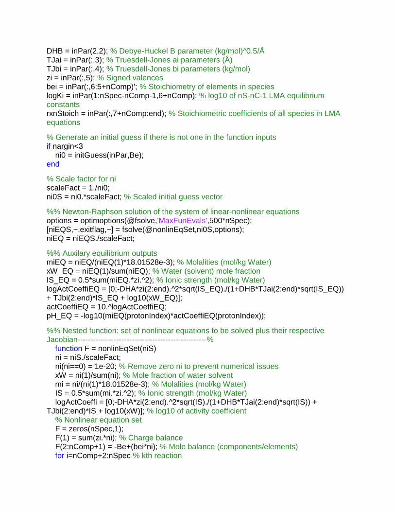
DHB = inPar(2,2); % Debye-Huckel B parameter (kg/mol)^0.5/Å
TJai = inPar(:,3); % Truesdell-Jones ai parameters (Å)
TJbi = inPar(:,4); % Truesdell-Jones bi parameters (kg/mol)
zi = inPar(:,5); % Signed valences
bei = inPar(:,6:5+nComp)'; % Stoichiometry of elements in species
logKi = inPar(1:nSpec-nComp-1,6+nComp); % log10 of nS-nC-1 LMA equilibrium constants
rxnStoich = inPar(:,7+nComp:end); % Stoichiometric coefficients of all species in LMA equations % Generate an initial guess if there is not one in the function inputs
if nargin<3
ni0 = initGuess(inPar,Be); end
% Scale factor for ni scaleFact = 1./ni0; ni0S = ni0.*scaleFact; % Scaled initial guess vector
%% Newton-Raphson solution of the system of linear-nonlinear equations
options = optimoptions(@fsolve,'MaxFunEvals',500*nSpec); [niEQS,~,exitflag,~] = fsolve(@nonlinEqSet,ni0S,options); niEQ = niEQS./scaleFact; %% Auxilary equilibrium outputs
miEQ = niEQ/(niEQ(1)*18.01528e-3); % Molalities (mol/kg Water)
xW_EQ = niEQ(1)/sum(niEQ); % Water (solvent) mole fraction
IS_EQ = 0.5*sum(miEQ.*zi.^2); % Ionic strength (mol/kg Water)
logActCoeffiEQ = [0;-DHA*zi(2:end).^2*sqrt(IS_EQ)./(1+DHB*TJai(2:end)*sqrt(IS_EQ)) + TJbi(2:end)*IS_EQ + log10(xW_EQ)]; actCoeffiEQ = 10.^logActCoeffiEQ; pH_EQ = -log10(miEQ(protonIndex)*actCoeffiEQ(protonIndex));
%% Nested function: set of nonlinear equations to be solved plus their respective Jacobian--------------------------------------------------%
function F = nonlinEqSet(niS)
ni = niS./scaleFact; ni(ni==0) = 1e-20; % Remove zero ni to prevent numerical issues
xW = ni(1)/sum(ni); % Mole fraction of water solvent mi = ni/(ni(1)*18.01528e-3); % Molalities (mol/kg Water)
IS = 0.5*sum(mi.*zi.^2); % Ionic strength (mol/kg Water)
logActCoeffi = [0;-DHA*zi(2:end).^2*sqrt(IS)./(1+DHB*TJai(2:end)*sqrt(IS)) + TJbi(2:end)*IS + log10(xW)]; % log10 of activity coefficient % Nonlinear equation set F = zeros(nSpec,1); F(1) = sum(zi.*ni); % Charge balance
F(2:nComp+1) = -Be+(bei*ni); % Mole balance (components/elements)
for i=nComp+2:nSpec % kth reaction
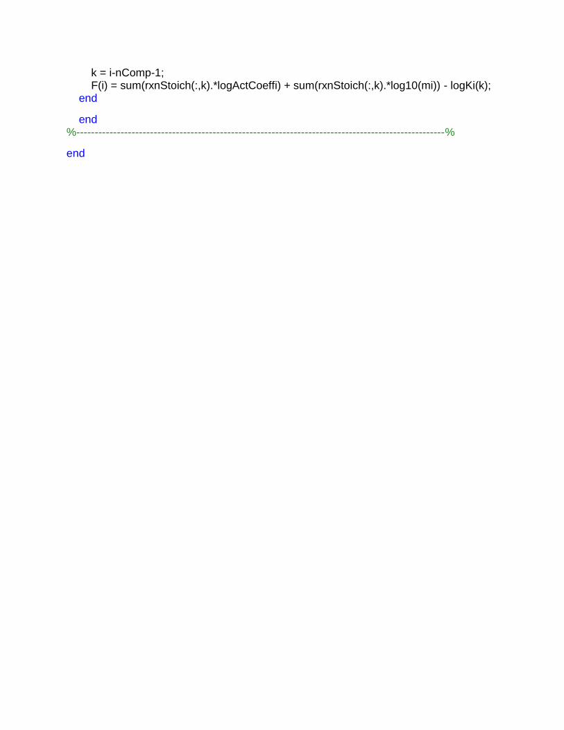
k = i-nComp-1; F(i) = sum(rxnStoich(:,k).*logActCoeffi) + sum(rxnStoich(:,k).*log10(mi)) - logKi(k); end
end
%----------------------------------------------------------------------------------------------------%
end
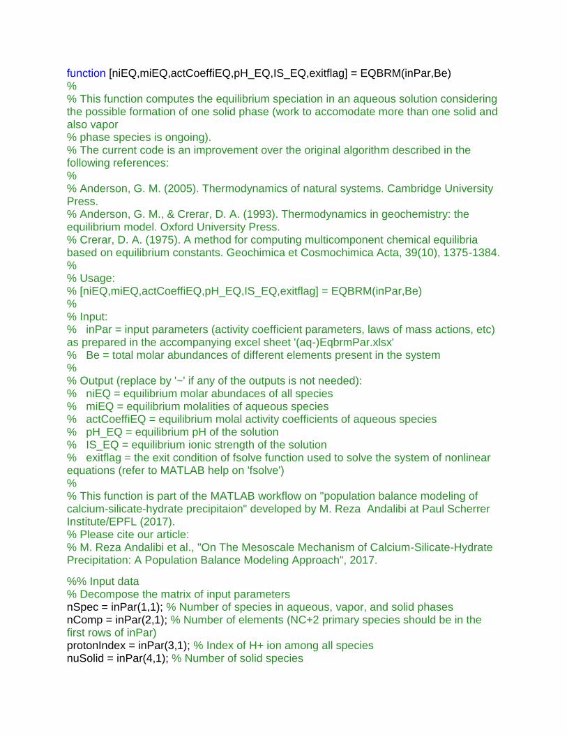
function [niEQ,miEQ,actCoeffiEQ,pH_EQ,IS_EQ,exitflag] = EQBRM(inPar,Be)
% % This function computes the equilibrium speciation in an aqueous solution considering the possible formation of one solid phase (work to accomodate more than one solid and also vapor
% phase species is ongoing). % The current code is an improvement over the original algorithm described in the following references: % % Anderson, G. M. (2005). Thermodynamics of natural systems. Cambridge University Press. % Anderson, G. M., & Crerar, D. A. (1993). Thermodynamics in geochemistry: the equilibrium model. Oxford University Press. % Crerar, D. A. (1975). A method for computing multicomponent chemical equilibria based on equilibrium constants. Geochimica et Cosmochimica Acta, 39(10), 1375-1384. % % Usage: % [niEQ,miEQ,actCoeffiEQ,pH_EQ,IS_EQ,exitflag] = EQBRM(inPar,Be)
% % Input: % inPar = input parameters (activity coefficient parameters, laws of mass actions, etc) as prepared in the accompanying excel sheet '(aq-)EqbrmPar.xlsx' % Be = total molar abundances of different elements present in the system
% % Output (replace by '~' if any of the outputs is not needed): % niEQ = equilibrium molar abundaces of all species
% miEQ = equilibrium molalities of aqueous species
% actCoeffiEQ = equilibrium molal activity coefficients of aqueous species
% pH_EQ = equilibrium pH of the solution
% IS_EQ = equilibrium ionic strength of the solution
% exitflag = the exit condition of fsolve function used to solve the system of nonlinear equations (refer to MATLAB help on 'fsolve')
% % This function is part of the MATLAB workflow on "population balance modeling of calcium-silicate-hydrate precipitaion" developed by M. Reza Andalibi at Paul Scherrer Institute/EPFL (2017). % Please cite our article: % M. Reza Andalibi et al., "On The Mesoscale Mechanism of Calcium-Silicate-Hydrate Precipitation: A Population Balance Modeling Approach", 2017. %% Input data
% Decompose the matrix of input parameters
nSpec = inPar(1,1); % Number of species in aqueous, vapor, and solid phases
nComp = inPar(2,1); % Number of elements (NC+2 primary species should be in the first rows of inPar)
protonIndex = inPar(3,1); % Index of H+ ion among all species
nuSolid = inPar(4,1); % Number of solid species

nuVap = inPar(5,1); % Number of species in vapor phase
nuAq = nSpec-nuSolid-nuVap; % Number of aqueous species
DHA = inPar(1,2); % Debye-Huckel A parameter (kg/mol)^0.5
DHB = inPar(2,2); % Debye-Huckel B parameter (kg/mol)^0.5/Å
TJai = inPar(1:nuAq,3); % Truesdell-Jones ai parameters (Å)
TJbi = inPar(1:nuAq,4); % Truesdell-Jones bi parameters (kg/mol)
zi = inPar(1:nuAq,5); % Signed valences
bei = inPar(:,6:5+nComp)'; % Stoichiometry of elements in species
logKi = inPar(1:nSpec-nComp-1,6+nComp); % log10 of nS-nC-1 LMA equilibrium constants
rxnStoich = inPar(:,7+nComp:end); % Stoichiometric coefficients of all species in LMA equations
%% Initial guess generation
% Aqueous equilibrium calculation
% Deriving inParAq from inPar
inParAq = inPar(1:nuAq,1:end-nuSolid-nuVap); inParAq(1,1) = nuAq; inParAq(4:end,1) = 0; inParAq(nuAq-nComp:end,6+nComp) = 0; [niAQ,miAQ,actCoeffiAQ,pH_AQ,IS_AQ,exitflag] = aqEQBRM(inParAq,Be);
ni0 = [niAQ;zeros(nuSolid,1)]; % Initial guess if system is not much supersaturated
% Saturation index check and possibly re-calculations considering SLE
SI = zeros(nuSolid,1); % Saturation index
for i=1:nuSolid
SI(i,1) = sum(rxnStoich(1:nuAq,end-nuSolid-nuVap+i).*log10(miAQ))... + sum(rxnStoich(1:nuAq,end-nuSolid-nuVap+i).*log10(actCoeffiAQ)) - logKi(end-nuSolid-nuVap+i,1); end
[maxSI,maxSI_index] = max(SI); if maxSI <=0 % (under-)saturated system
niEQ = [niAQ;0]; % Zero mole amount for undersaturated solid
miEQ = miAQ; actCoeffiEQ = actCoeffiAQ; pH_EQ = pH_AQ; IS_EQ = IS_AQ; elseif (0<maxSI) && (maxSI<=0.1) % Slightly supersaturated system
ni0(maxSI_index+nuAq) = 0; % Initial guess for solid mole amount % Newton-Raphson solution using the generated initial guess (SLE)
alphaS = 1./ni0; alphaS(alphaS==Inf) = 1; % Correcting for division by zero
ni0S = ni0.*alphaS; options = optimoptions(@fsolve,'MaxFunEvals',1000*nSpec,'MaxIter',500); [niEQscaled,~,exitflag,~] = fsolve(@nonlinEqSet,ni0S,options); niEQ = niEQscaled./alphaS; % Auxilary equilibrium outputs
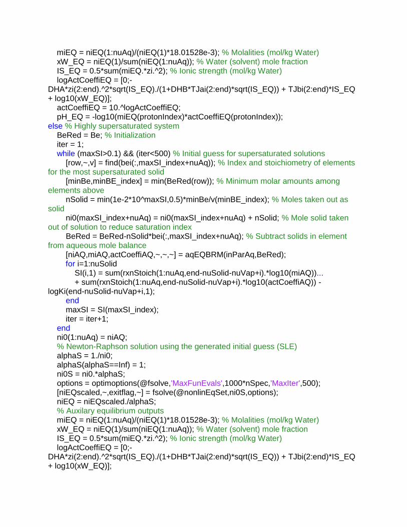
miEQ = niEQ(1:nuAq)/(niEQ(1)*18.01528e-3); % Molalities (mol/kg Water)
xW_EQ = niEQ(1)/sum(niEQ(1:nuAq)); % Water (solvent) mole fraction
IS_EQ = 0.5*sum(miEQ.*zi.^2); % Ionic strength (mol/kg Water)
logActCoeffiEQ = [0;-DHA*zi(2:end).^2*sqrt(IS_EQ)./(1+DHB*TJai(2:end)*sqrt(IS_EQ)) + TJbi(2:end)*IS_EQ + log10(xW_EQ)]; actCoeffiEQ = 10.^logActCoeffiEQ; pH_EQ = -log10(miEQ(protonIndex)*actCoeffiEQ(protonIndex)); else % Highly supersaturated system
BeRed = Be; % Initialization
iter = 1; while (maxSI>0.1) && (iter<500) % Initial guess for supersaturated solutions
[row,~,v] = find(bei(:,maxSI_index+nuAq)); % Index and stoichiometry of elements for the most supersaturated solid
[minBe,minBE_index] = min(BeRed(row)); % Minimum molar amounts among elements above
nSolid = min(1e-2*10^maxSI,0.5)*minBe/v(minBE_index); % Moles taken out as solid
ni0(maxSI_index+nuAq) = ni0(maxSI_index+nuAq) + nSolid; % Mole solid taken out of solution to reduce saturation index
BeRed = BeRed-nSolid*bei(:,maxSI_index+nuAq); % Subtract solids in element from aqueous mole balance
[niAQ,miAQ,actCoeffiAQ,~,~,~] = aqEQBRM(inParAq,BeRed); for i=1:nuSolid
SI(i,1) = sum(rxnStoich(1:nuAq,end-nuSolid-nuVap+i).*log10(miAQ))... + sum(rxnStoich(1:nuAq,end-nuSolid-nuVap+i).*log10(actCoeffiAQ)) - logKi(end-nuSolid-nuVap+i,1); end
maxSI = SI(maxSI_index); iter = iter+1; end
ni0(1:nuAq) = niAQ; % Newton-Raphson solution using the generated initial guess (SLE)
alphaS = 1./ni0; alphaS(alphaS==Inf) = 1; ni0S = ni0.*alphaS; options = optimoptions(@fsolve,'MaxFunEvals',1000*nSpec,'MaxIter',500); [niEQscaled,~,exitflag,~] = fsolve(@nonlinEqSet,ni0S,options); niEQ = niEQscaled./alphaS; % Auxilary equilibrium outputs
miEQ = niEQ(1:nuAq)/(niEQ(1)*18.01528e-3); % Molalities (mol/kg Water)
xW_EQ = niEQ(1)/sum(niEQ(1:nuAq)); % Water (solvent) mole fraction
IS_EQ = 0.5*sum(miEQ.*zi.^2); % Ionic strength (mol/kg Water)
logActCoeffiEQ = [0;-DHA*zi(2:end).^2*sqrt(IS_EQ)./(1+DHB*TJai(2:end)*sqrt(IS_EQ)) + TJbi(2:end)*IS_EQ + log10(xW_EQ)];
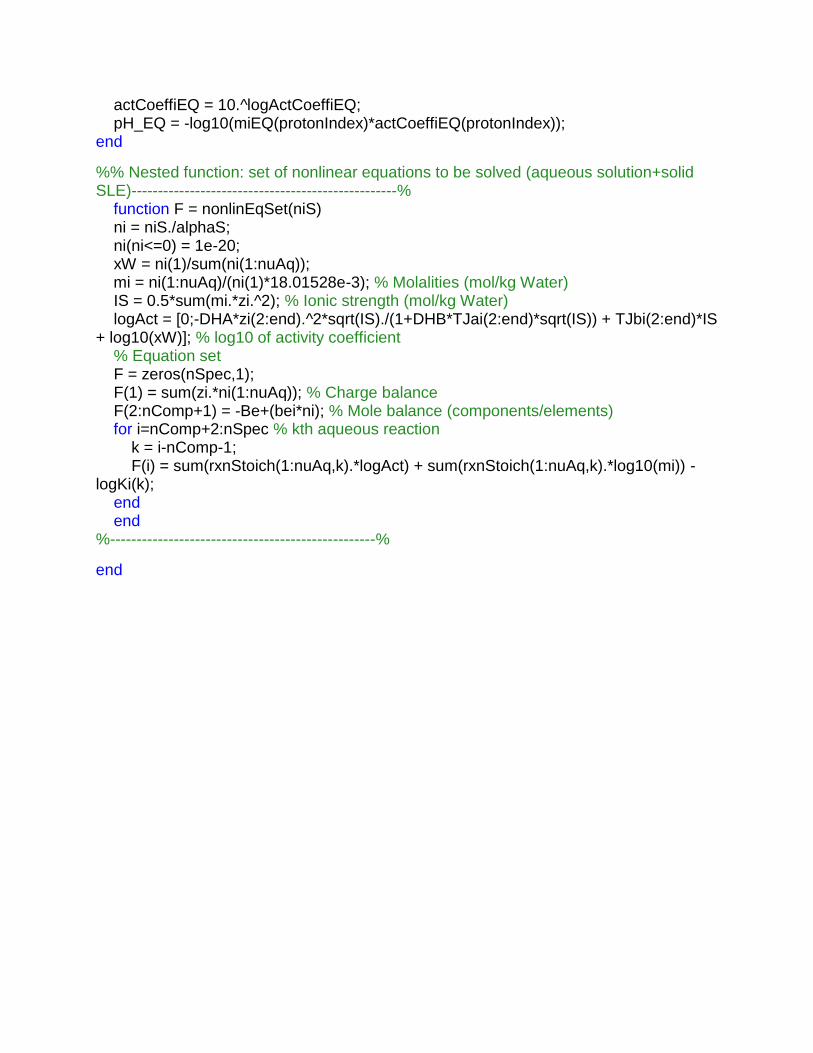
actCoeffiEQ = 10.^logActCoeffiEQ; pH_EQ = -log10(miEQ(protonIndex)*actCoeffiEQ(protonIndex)); end
%% Nested function: set of nonlinear equations to be solved (aqueous solution+solid SLE)--------------------------------------------------%
function F = nonlinEqSet(niS)
ni = niS./alphaS; ni(ni<=0) = 1e-20; xW = ni(1)/sum(ni(1:nuAq)); mi = ni(1:nuAq)/(ni(1)*18.01528e-3); % Molalities (mol/kg Water)
IS = 0.5*sum(mi.*zi.^2); % Ionic strength (mol/kg Water)
logAct = [0;-DHA*zi(2:end).^2*sqrt(IS)./(1+DHB*TJai(2:end)*sqrt(IS)) + TJbi(2:end)*IS + log10(xW)]; % log10 of activity coefficient % Equation set F = zeros(nSpec,1); F(1) = sum(zi.*ni(1:nuAq)); % Charge balance
F(2:nComp+1) = -Be+(bei*ni); % Mole balance (components/elements)
for i=nComp+2:nSpec % kth aqueous reaction
k = i-nComp-1; F(i) = sum(rxnStoich(1:nuAq,k).*logAct) + sum(rxnStoich(1:nuAq,k).*log10(mi)) - logKi(k); end
end
%--------------------------------------------------%
end
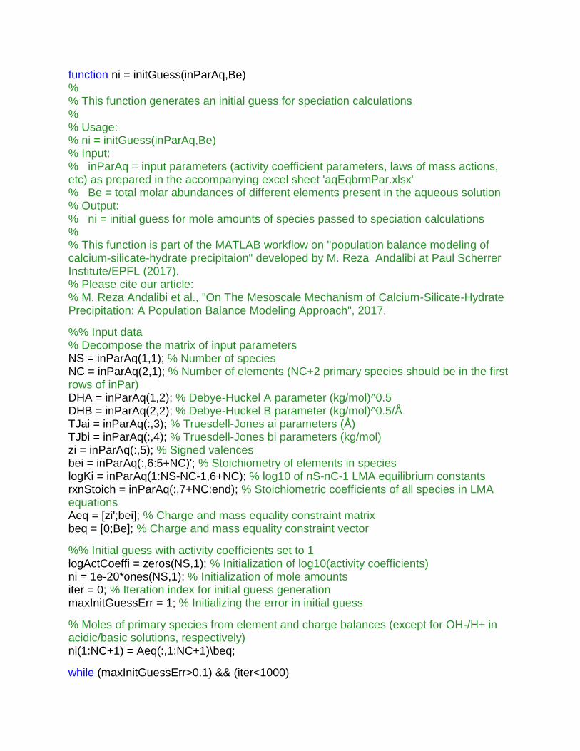
function ni = initGuess(inParAq,Be)
% % This function generates an initial guess for speciation calculations
% % Usage: % ni = initGuess(inParAq,Be)
% Input: % inParAq = input parameters (activity coefficient parameters, laws of mass actions, etc) as prepared in the accompanying excel sheet 'aqEqbrmPar.xlsx' % Be = total molar abundances of different elements present in the aqueous solution
% Output: % ni = initial guess for mole amounts of species passed to speciation calculations
% % This function is part of the MATLAB workflow on "population balance modeling of calcium-silicate-hydrate precipitaion" developed by M. Reza Andalibi at Paul Scherrer Institute/EPFL (2017). % Please cite our article: % M. Reza Andalibi et al., "On The Mesoscale Mechanism of Calcium-Silicate-Hydrate Precipitation: A Population Balance Modeling Approach", 2017. %% Input data
% Decompose the matrix of input parameters
NS = inParAq(1,1); % Number of species
NC = inParAq(2,1); % Number of elements (NC+2 primary species should be in the first rows of inPar)
DHA = inParAq(1,2); % Debye-Huckel A parameter (kg/mol)^0.5
DHB = inParAq(2,2); % Debye-Huckel B parameter (kg/mol)^0.5/Å
TJai = inParAq(:,3); % Truesdell-Jones ai parameters (Å)
TJbi = inParAq(:,4); % Truesdell-Jones bi parameters (kg/mol)
zi = inParAq(:,5); % Signed valences
bei = inParAq(:,6:5+NC)'; % Stoichiometry of elements in species
logKi = inParAq(1:NS-NC-1,6+NC); % log10 of nS-nC-1 LMA equilibrium constants
rxnStoich = inParAq(:,7+NC:end); % Stoichiometric coefficients of all species in LMA equations Aeq = [zi';bei]; % Charge and mass equality constraint matrix
beq = [0;Be]; % Charge and mass equality constraint vector
%% Initial guess with activity coefficients set to 1
logActCoeffi = zeros(NS,1); % Initialization of log10(activity coefficients)
ni = 1e-20*ones(NS,1); % Initialization of mole amounts
iter = 0; % Iteration index for initial guess generation
maxInitGuessErr = 1; % Initializing the error in initial guess
% Moles of primary species from element and charge balances (except for OH-/H+ in acidic/basic solutions, respectively)
ni(1:NC+1) = Aeq(:,1:NC+1)\beq; while (maxInitGuessErr>0.1) && (iter<1000)
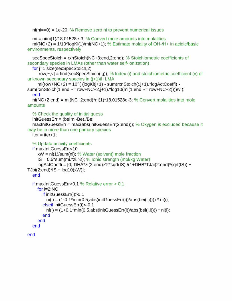
ni(ni==0) = 1e-20; % Remove zero ni to prevent numerical issues
mi = ni/ni(1)/18.01528e-3; % Convert mole amounts into molalities
mi(NC+2) = 1/10^logKi(1)/mi(NC+1); % Estimate molality of OH-/H+ in acidic/basic environments, respectively
secSpecStoich = rxnStoich(NC+3:end,2:end); % Stoichiometric coefficients of secondary species in LMAs (other than water self-ionization)
for j=1:size(secSpecStoich,2)
[row,~,v] = find(secSpecStoich(:,j)); % Index (i) and stoichiometric coefficient (v) of unknown secondary species in (j+1)th LMA
mi(row+NC+2) = 10^( (logKi(j+1) - sum(rxnStoich(:,j+1).*logActCoeffi) - sum(rxnStoich(1:end ~= row+NC+2,j+1).*log10(mi(1:end ~= row+NC+2))))/v );
end
ni(NC+2:end) = mi(NC+2:end)*ni(1)*18.01528e-3; % Convert molalities into mole amounts
% Check the quality of initial guess
initGuessErr = (bei*ni-Be)./Be; maxInitGuessErr = max(abs(initGuessErr(2:end))); % Oxygen is excluded because it may be in more than one primary species
iter = iter+1; % Updata activity coefficients
if maxInitGuessErr<10
xW = ni(1)/sum(ni); % Water (solvent) mole fraction
IS = 0.5*sum(mi.*zi.^2); % Ionic strength (mol/kg Water)
logActCoeffi = [0;-DHA*zi(2:end).^2*sqrt(IS)./(1+DHB*TJai(2:end)*sqrt(IS)) + TJbi(2:end)*IS + log10(xW)]; end
if maxInitGuessErr>0.1 % Relative error > 0.1
for i=2:NC
if initGuessErr(i)>0.1
ni(i) = (1-0.1*min(0.5,abs(initGuessErr(i))/abs(bei(i,i)))) * ni(i); elseif initGuessErr(i)<-0.1
ni(i) = (1+0.1*min(0.5,abs(initGuessErr(i))/abs(bei(i,i)))) * ni(i);
end
end
end
end

% This script calculates aqEQBRM data for C-S-H precipitation system and is part of the MATLAB workflow on
% "population balance modeling of calcium-silicate-hydrate precipitaion" developed by M. Reza Andalibi at Paul Scherrer Institute/EPFL (2017). % Please cite our article: % M. Reza Andalibi et al., "On The Mesoscale Mechanism of Calcium-Silicate-Hydrate Precipitation: A Population Balance Modeling Approach", 2017. clear; clc; inParAq = dlmread('inParAq.txt'); Be = dlmread('Be_2.0mL.min-1.txt'); % Be = dlmread('Be_0.5mL.min-1.txt'); eqNo = size(Be,1); niEQ = zeros(eqNo,15); miEQ = zeros(eqNo,15); actCoeffiEQ = zeros(eqNo,15); pH_EQ = zeros(eqNo,1); IS_EQ = zeros(eqNo,1); exitflag = zeros(eqNo,1); % parfor j=1:eqNo % If initial guesses are not available parallelization can expedite the computation
% [niEQ(j,:),miEQ(j,:),actCoeffiEQ(j,:),pH_EQ(j,1),IS_EQ(j,1),exitflag(j,1)] = aqEQBRM(inPar,Be(j,:)'); % end
j=1; [niEQ(j,:),miEQ(j,:),actCoeffiEQ(j,:),pH_EQ(j,1),IS_EQ(j,1),exitflag(j,1)] = aqEQBRM(inParAq,Be(j,:)'); for j=2:eqNo
[niEQ(j,:),miEQ(j,:),actCoeffiEQ(j,:),pH_EQ(j,1),IS_EQ(j,1),exitflag(j,1)] = aqEQBRM(inParAq,Be(j,:)',niEQ(j-1,:)'); end
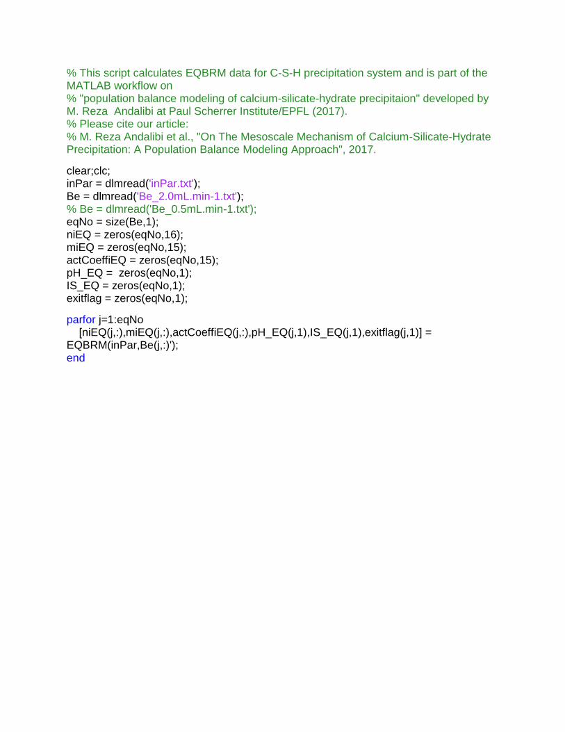
% This script calculates EQBRM data for C-S-H precipitation system and is part of the MATLAB workflow on
% "population balance modeling of calcium-silicate-hydrate precipitaion" developed by M. Reza Andalibi at Paul Scherrer Institute/EPFL (2017). % Please cite our article: % M. Reza Andalibi et al., "On The Mesoscale Mechanism of Calcium-Silicate-Hydrate Precipitation: A Population Balance Modeling Approach", 2017. clear;clc; inPar = dlmread('inPar.txt'); Be = dlmread('Be_2.0mL.min-1.txt'); % Be = dlmread('Be_0.5mL.min-1.txt'); eqNo = size(Be,1); niEQ = zeros(eqNo,16); miEQ = zeros(eqNo,15); actCoeffiEQ = zeros(eqNo,15); pH_EQ = zeros(eqNo,1); IS_EQ = zeros(eqNo,1); exitflag = zeros(eqNo,1); parfor j=1:eqNo
[niEQ(j,:),miEQ(j,:),actCoeffiEQ(j,:),pH_EQ(j,1),IS_EQ(j,1),exitflag(j,1)] = EQBRM(inPar,Be(j,:)'); end
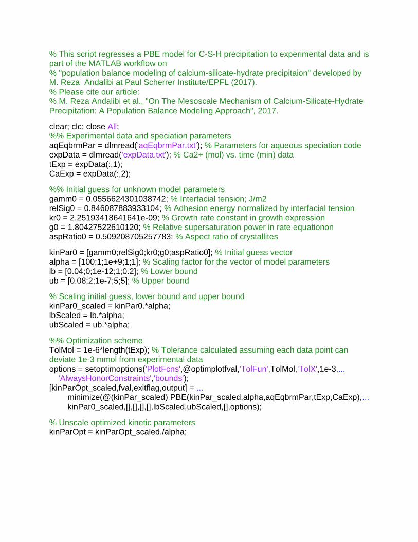
% This script regresses a PBE model for C-S-H precipitation to experimental data and is part of the MATLAB workflow on
% "population balance modeling of calcium-silicate-hydrate precipitaion" developed by M. Reza Andalibi at Paul Scherrer Institute/EPFL (2017). % Please cite our article: % M. Reza Andalibi et al., "On The Mesoscale Mechanism of Calcium-Silicate-Hydrate Precipitation: A Population Balance Modeling Approach", 2017. clear; clc; close All; %% Experimental data and speciation parameters
aqEqbrmPar = dlmread('aqEqbrmPar.txt'); % Parameters for aqueous speciation code
expData = dlmread('expData.txt'); % Ca2+ (mol) vs. time (min) data
tExp = expData(:,1); CaExp = expData(:,2); %% Initial guess for unknown model parameters
gamm0 = 0.0556624301038742; % Interfacial tension; J/m2
relSig0 = 0.846087883933104; % Adhesion energy normalized by interfacial tension
kr0 = 2.25193418641641e-09; % Growth rate constant in growth expression
g0 = 1.80427522610120; % Relative supersaturation power in rate equationon
aspRatio0 = 0.509208705257783; % Aspect ratio of crystallites
kinPar0 = [gamm0;relSig0;kr0;g0;aspRatio0]; % Initial guess vector
alpha = [100;1;1e+9;1;1]; % Scaling factor for the vector of model parameters
lb = [0.04;0;1e-12;1;0.2]; % Lower bound
ub = [0.08;2;1e-7;5;5]; % Upper bound
% Scaling initial guess, lower bound and upper bound
kinPar0_scaled = kinPar0.*alpha; lbScaled = lb.*alpha; ubScaled = ub.*alpha; %% Optimization scheme
TolMol = 1e-6*length(tExp); % Tolerance calculated assuming each data point can deviate 1e-3 mmol from experimental data
options = setoptimoptions('PlotFcns',@optimplotfval,'TolFun',TolMol,'TolX',1e-3,... 'AlwaysHonorConstraints','bounds'); [kinParOpt_scaled,fval,exitflag,output] = ... minimize(@(kinPar_scaled) PBE(kinPar_scaled,alpha,aqEqbrmPar,tExp,CaExp),... kinPar0_scaled,[],[],[],[],lbScaled,ubScaled,[],options); % Unscale optimized kinetic parameters
kinParOpt = kinParOpt_scaled./alpha;
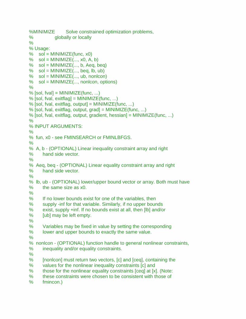
%MINIMIZE Solve constrained optimization problems, % globally or locally
%
% Usage: % sol = MINIMIZE(func, x0) % sol = MINIMIZE(..., x0, A, b) % sol = MINIMIZE(..., b, Aeq, beq) % sol = MINIMIZE(..., beq, lb, ub)
% sol = MINIMIZE(..., ub, nonlcon) % sol = MINIMIZE(..., nonlcon, options) %
% [sol, fval] = MINIMIZE(func, ...)
% [sol, fval, exitflag] = MINIMIZE(func, ...)
% [sol, fval, exitflag, output] = MINIMIZE(func, ...)
% [sol, fval, exitflag, output, grad] = MINIMIZE(func, ...)
% [sol, fval, exitflag, output, gradient, hessian] = MINIMIZE(func, ...)
%
% INPUT ARGUMENTS: %
% fun, x0 - see FMINSEARCH or FMINLBFGS. %
% A, b - (OPTIONAL) Linear inequality constraint array and right % hand side vector. %
% Aeq, beq - (OPTIONAL) Linear equality constraint array and right % hand side vector. %
% lb, ub - (OPTIONAL) lower/upper bound vector or array. Both must have % the same size as x0. %
% If no lower bounds exist for one of the variables, then
% supply -inf for that variable. Similarly, if no upper bounds % exist, supply +inf. If no bounds exist at all, then [lb] and/or % [ub] may be left empty. %
% Variables may be fixed in value by setting the corresponding
% lower and upper bounds to exactly the same value. %
% nonlcon - (OPTIONAL) function handle to general nonlinear constraints, % inequality and/or equality constraints. %
% [nonlcon] must return two vectors, [c] and [ceq], containing the
% values for the nonlinear inequality constraints [c] and
% those for the nonlinear equality constraints [ceq] at [x]. (Note: % these constraints were chosen to be consistent with those of % fmincon.)
%
% options - (OPTIONAL) an options structure created manually or with
% setoptimoptions(). % % OUTPUT ARGUMENTS: %
% sol, fval - the solution vector and the corresponding function value,
% respectively. %
% exitflag - (See also the help on FMINSEARCH) A flag that specifies the % reason the algorithm terminated. FMINSEARCH uses only the values
%
% 1 fminsearch converged to a solution x
% 0 Max. # of function evaluations or iterations exceeded
% -1 Algorithm was terminated by the output function. %
% Since MINIMIZE handles constrained problems, the following % values were added: %
% 2 Problem overconstrained by either [lb]/[ub] or
% [Aeq]/[beq] - nothing done
% -2 Problem is infeasible after the optimization (Some or % any of the constraints are violated at the final % solution). % -3 INF or NAN encountered during the optimization. %
% output - (See also the help on FMINSEARCH) A structure that contains
% additional details on the optimization. %
% Notes: %
% If [options] is supplied, then TolX will apply to the transformed
% variables. All other FMINSEARCH parameters should be unaffected. %
%
% EXAMPLES: %
% rosen = @(x) (1-x(1)).^2 + 105*(x(2)-x(1).^2).^2; %
% >> % Fully unconstrained problem
% >> minimize(rosen, [3 3])
% ans =
% 1.0000 1.0000
%
%
% >> % lower bound constrained
% >> minimize(rosen,[3 3], [],[], [],[], [2 2])
% ans =
% 2.0000 4.0000
%
%
% >> % x(2) fixed at 3
% >> minimize(rosen,[3 3], [],[], [],[], [-inf 3],[inf,3])
% ans =
% 1.7314 3.0000
%
%
% >> % simple linear inequality: x(1) + x(2) <= 1
% >> minimize(rosen,[0; 0], [1 1], 1)
% % ans =
% 0.6187 0.3813
% %
% >> % nonlinear inequality: sqrt(x(1)^2 + x(2)^2) <= 1
% >> % nonlinear equality : x(1)^2 + x(2)^3 = 0.5
%
% Execute this m-file: %
% function test_minimize
% rosen = @(x) (1-x(1)).^2 + 105*(x(2)-x(1).^2).^2; %
% options = optimset('TolFun', 1e-8, 'TolX', 1e-8); %
% minimize(rosen, [3 3], [],[],[],[],[],[],... % @nonlcon, [], options)
%
% end
% function [c, ceq] = nonlcon(x)
% c = norm(x) - 1; % ceq = x(1)^2 + x(2)^3 - 0.5; % end
%
% ans =
% 0.6513 0.4233
%
%
% Of course, any combination of the above constraints is
% also possible. %
%
% See also: SETOPTIMOPTIONS, FMINSEARCH, FMINLBFGS.
% Please report bugs and inquiries to: %
% Name : Rody P.S. Oldenhuis
% E-mail : [email protected] (personal)
% [email protected] (professional)
% Affiliation: LuxSpace sàrl % Licence : BSD
% FMINSEARCHBND, FMINSEARCHCON and part of the documentation % for MINIMIZE witten by
%
% Author : John D'Errico
% E-mail : [email protected]
% TODO
%{
WISH: Transformations similar to the ones used for bound constraints should
also be possible for linear constraints; figure this out. WISH: more checks for inconsistent constraints: - equality constraints might all lie outside the region defined by the bounds and linear inequalities
- different linear equality constraints might never intersect WISH: Include examples and demos in the documentation
WISH: a properly working ConstraintsInObjectiveFunction
FIXME: check how functions are evaluated; isn't it better to have objFcn()
and conFcn() do more work? FIXME: ignore given nonlcon() if ConstraintsInObjectiveFunction is true?
FIXME: fevals is miscounted; possibly fminlbfgs bug
FIXME: TolX, TolFun, TolCon, DiffMinchange, DiffMaxChange should be transformed
FIXME: 'AlwaysHonorConstraints' == 'bounds' does nothing
%}
function [sol, fval, exitflag, output, grad] = ... minimize(funfcn, x0, A,b, Aeq,beq, lb,ub, nonlcon, options, varargin)
% If you find this work useful, please consider a donation: % https://www.paypal.com/cgi-bin/webscr?cmd=_s-xclick&hosted_button_id=6G3S5UYM7HJ3N
%% Initialization
% Process user input narg = nargin; if verLessThan('MATLAB', '8.6')
error(nargchk(2, inf, narg, 'struct')); %#ok<NCHKN>
error(nargchk(0, 6, nargout, 'struct')); %#ok<NCHKM>
else
narginchk (2, inf); nargoutchk(0, 6); end
if (narg < 10) || isempty(options), options = setoptimoptions; end
if (narg < 9), nonlcon = ''; end
if (narg < 8), ub = []; end
if (narg < 7), lb = []; end
if (narg < 6), beq = []; end
if (narg < 5), Aeq = []; end
if (narg < 4), b = []; end
if (narg < 3), A = []; end
% Extract options
nonlconFcn_in_objFcn = getoptimoptions('ConstraintsInObjectiveFunction', false); tolCon = getoptimoptions('TolCon', 1e-8); algorithm = getoptimoptions('Algorithm', 'fminsearch'); strictness = getoptimoptions('AlwaysHonorConstraints', 'none'); diffMinChange = getoptimoptions('DiffMinChange', 1e-8); diffMaxChange = getoptimoptions('DiffMaxChange', 1e-1); finDiffType = getoptimoptions('FinDiffType', 'forward'); OutputFcn = getoptimoptions('OutputFcn', []); PlotFcn = getoptimoptions('PlotFcn', []); % Set some logicals for easier reading
have_nonlconFcn = ~isempty(nonlcon) || nonlconFcn_in_objFcn;
have_linineqconFcn = ~isempty(A) && ~isempty(b); have_lineqconFcn = ~isempty(Aeq) && ~isempty(beq); create_output = (nargout >= 4); need_grad = strcmpi(algorithm,'fminlbfgs'); grad_obj_from_objFcn = need_grad && strcmpi(options.GradObj ,'on'); grad_nonlcon_from_nonlconFcn = need_grad && strcmpi(options.GradConstr,'on') && have_nonlconFcn; do_display = ~isempty(options.Display) && ~strcmpi(options.Display,'off'); do_extended_display = do_display && strcmpi(options.Display,'iter-detailed'); do_global_opt = isempty(x0); % Do we have an output function? have_outputFcn = ~isempty(OutputFcn); have_plotFcn = ~isempty(PlotFcn); % No x0 given means minimize globally.
if do_global_opt [sol, fval, exitflag, output] = minimize_globally();
return; end
% Make copy of UNpenalized function value
UPfval = inf; % Initialize & define constants superstrict = false; % initially, don't use superstrict setting exp50 = exp(50); % maximum penalty
N0 = numel(x0); % variable to check sizes etc. Nzero = zeros(N0, 1); % often-used zero-matrix grad = []; % initially, nothing for gradient sumAT = repmat(sum(A,1).',1,size(b,2)); % column-sum of [A] , transposed and replicated
sumAeqT = repmat(sum(Aeq,1).',1,size(beq,2)); % column-sum of [Aeq], transposed and replicated
% Initialize output structure
output = []; if create_output % Fields always present output.iterations = 0; output.algorithm = ''; output.message = 'Initializing optimization...'; % Fields present depending on the presence of nonlcon
if ~have_nonlconFcn
output.funcCount = 0; else
output.ObjfuncCount = 0; output.ConstrfuncCount = 1; % one evaluation in check_input()
output.constrviolation.nonlin_eq = cell(2,1); output.constrviolation.nonlin_ineq = cell(2,1); end
% Fields present depending on the presence of A or Aeq
if have_linineqconFcn
output.constrviolation.lin_ineq = cell(2,1); end
if have_lineqconFcn
output.constrviolation.lin_eq = cell(2,1); end
end
% Save variable with original size new_x = x0; % Check for an output/plot functions. If there are any,
% use wrapper functions to call it with un-transformed variable
if have_outputFcn
OutputFcn = options.OutputFcn; if ~iscell(OutputFcn)
OutputFcn = {OutputFcn}; end
options.OutputFcn = @OutputFcn_wrapper; end if have_plotFcn
PlotFcn = options.PlotFcn; if ~iscell(PlotFcn)
PlotFcn = {PlotFcn}; end
options.PlotFcn = @PlotFcn_wrapper; end % Adjust bounds when they are empty
if isempty(lb), lb = -inf(size(x0)); end
if isempty(ub), ub = +inf(size(x0)); end
% Check the user-provided input with nested function check_input checks_OK = check_input; if ~checks_OK, return; end % Force everything to be column vector
ub = ub(:); x0 = x0(:); lb = lb(:); x0one = ones(size(x0)); % replicate lb or ub when they are scalars, and x0 is not if isscalar(lb) && (N0 ~= 1), lb = lb*x0one; end
if isscalar(ub) && (N0 ~= 1), ub = ub*x0one; end % Determine the type of bounds
nf_lb = ~isfinite(lb); nf_ub = ~isfinite(ub); fix_var = lb == ub; lb_only = ~nf_lb & nf_ub & ~fix_var;
ub_only = nf_lb & ~nf_ub & ~fix_var; unconst = nf_lb & nf_ub & ~fix_var;
lb_ub = ~nf_lb & ~nf_ub & ~fix_var; %% Optimization % Force the initial estimate inside the given bounds
x0(x0 < lb) = lb(x0 < lb); x0(x0 > ub) = ub(x0 > ub); % Transform initial estimate to its unconstrained counterpart xin = x0; % fixed and unconstrained variables xin(lb_only) = sqrt(x0(lb_only) - lb(lb_only)); % lower bounds only xin(ub_only) = sqrt(ub(ub_only) - x0(ub_only)); % upper bounds only
xin(lb_ub) = real(asin( 2*(x0(lb_ub) - lb(lb_ub))./ ... (ub(lb_ub) - lb(lb_ub)) - 1)); % both upper and lower bounds
xin(fix_var) = [];
% Some more often-used matrices
None = ones(numel(xin)+1,1); Np1zero = zeros(N0, numel(xin)+1); % Optimize the problem
try
switch lower(algorithm)
% MATLAB's own derivative-free Nelder-Mead algorithm (FMINSEARCH())
case 'fminsearch' [presol, fval, exitflag, output_a] = ... fminsearch(@funfcnT, xin, options); % Transform solution back to original (bounded) variables...
sol = new_x; sol(:) = X(presol); % with the same size as the original x0
% Evaluate function once more to get unconstrained values
% NOTE: this eval is added to total fevals later
fval(:) = objFcn(sol); % Steepest descent or Quasi-Newton (limited-memory) BFGS % (both using gradient) FMINLBFGS(), by Dirk-Jan Kroon case 'fminlbfgs' % DEBUG: check gradients
%{
% Numerical oneHundredth = [ ( funfcnT(xin+[1e-2;0])-funfcnT(xin-[1e-2;0]))/2e-2
( funfcnT(xin+[0;1e-2])-funfcnT(xin-[0;1e-2]))/2e-2] oneTrillionth = [ ( funfcnT(xin+[1e-12;0])-funfcnT(xin-[1e-12;0]))/2e-12
( funfcnT(xin+[0;1e-12])-funfcnT(xin-[0;1e-12]))/2e-12] h = 1e-3; dfdx = @(f,x) ( (f(x-4*h)-f(x+4*h))/280 + 4*(f(x+3*h)-f(x-3*h))/105 + (f(x-2*h)-f(x+2*h))/5 + 4*(f(x+h)-f(x-h))/5 )/h; %#ok
highOrder = [ dfdx(@(x)funfcnT([x;xin(2)]), xin(1)); dfdx(@(x)funfcnT([xin(1);x]), xin(2)) ] % As computed in penalized/transformed function
[F,G] = funfcnT(xin)
%}
[presol, fval, exitflag, output_a] = ... fminlbfgs(@funfcnT, xin, options); % Transform solution back to original (bounded) variables
sol = new_x; sol(:) = X(presol); % with the same size as the original x0 % Evaluate function some more to get unconstrained values
if grad_obj_from_objFcn
% Function value and gradient [fval, grad] = objFcn(sol); else
% Only function value
[fevals, grad] = computeJacobian(funfcn, sol, objFcn(sol)); if create_output output_a.funcCount = output_a.funcCount + fevals + 1; end
end
end % switch (algorithm)
catch ME ME2 = MException('minimize:unhandled_error',... 'Unhandled problem encountered; please contact the author with this exact message, and your exact inputs.'); throw(addCause(ME2,ME)); end
% Copy appropriate fields to the output structure
if create_output output.message = output_a.message; output.algorithm = output_a.algorithm; output.iterations = output_a.iterations; if ~have_nonlconFcn
output.funcCount = output_a.funcCount + 1; else output.ObjfuncCount = output_a.funcCount + 1; end
end
% Append constraint violations to the output structure, and change the
% exitflag accordingly
[output, exitflag] = finalize(sol, output, exitflag); %% NESTED FUNCTIONS (THE ACTUAL WORK)
% Check user-provided input function go_on = check_input % FIXME: diffMinChange and diffMaxChange can be inconsistent go_on = true; % Dimensions & weird input if (numel(lb) ~= N0 && ~isscalar(lb)) || (numel(ub) ~= N0 && ~isscalar(ub))
error('minimize:lb_ub_incompatible_size',...
'Size of either [lb] or [ub] incompatible with size of [x0].')
end
if ~isempty(A) && isempty(b)
warning('minimize:Aeq_but_not_beq', ... ['I received the matrix [A], but you omitted the corresponding vector [b].',... '\nI''ll assume a zero-vector for [b]...'])
b = zeros(size(A,1), size(x0,2)); end
if ~isempty(Aeq) && isempty(beq)
warning('minimize:Aeq_but_not_beq', ... ['I received the matrix [Aeq], but you omitted the corresponding vector [beq].',... '\nI''ll assume a zero-vector for [beq]...'])
beq = zeros(size(Aeq,1), size(x0,2)); end
if isempty(Aeq) && ~isempty(beq)
warning('minimize:beq_but_not_Aeq', ... ['I received the vector [beq], but you omitted the corresponding matrix [Aeq].',... '\nI''ll ignore the given [beq]...'])
beq = []; end
if isempty(A) && ~isempty(b)
warning('minimize:b_but_not_A', ... ['I received the vector [b], but you omitted the corresponding matrix [A].',... '\nI''ll ignore the given [b]...'])
b = []; end
if have_linineqconFcn && size(b,1)~=size(A,1)
error('minimize:b_incompatible_with_A',... 'The size of [b] is incompatible with that of [A].')
end
if have_lineqconFcn && size(beq,1)~=size(Aeq,1)
error('minimize:b_incompatible_with_A',... 'The size of [beq] is incompatible with that of [Aeq].')
end
if ~isvector(x0) && ~isempty(A) && (size(A,2) ~= size(x0,1))
error('minimize:A_incompatible_size',... 'Linear constraint matrix [A] has incompatible size for given [x0].')
end
if ~isvector(x0) && ~isempty(Aeq) && (size(Aeq,2) ~= size(x0,1))
error('minimize:Aeq_incompatible_size',... 'Linear constraint matrix [Aeq] has incompatible size for given [x0].')
end
if ~isempty(b) && size(b,2)~=size(x0,2)
error('minimize:x0_vector_but_not_b',...
'Given linear constraint vector [b] has incompatible size with given [x0].')
end
if ~isempty(beq) && size(beq,2)~=size(x0,2)
error('minimize:x0_vector_but_not_beq',... 'Given linear constraint vector [beq] has incompatible size with given [x0].')
end % Functions are not function handles if ~isa(funfcn, 'function_handle')
error('minimize:func_not_a_function',... 'Objective function must be given as a function handle.')
end
if ~isempty(nonlcon) && ~ischar(nonlcon) && ~isa(nonlcon, 'function_handle')
error('minimize:nonlcon_not_a_function', ... 'non-linear constraint function must be a function handle (advised) or string (discouraged).')
end
% Check if FMINLBFGS can be executed
%FIXME: not required when you paste it as nested function below
% if ~isempty(algorithm) && strcmpi(algorithm,'fminlbfgs') && isempty(which('fminlbfgs'))
% error('minimize:fminlbfgs_not_present',... % 'The function FMINLBFGS is not present in the current MATLAB path.');
% end
% evaluate the non-linear constraint function on % the initial value, to perform initial checks
% FIXME: fevals not counted
grad_c = []; grad_ceq = []; [c, ceq] = conFcn(x0); % Check sizes of derivatives
if ~isempty(grad_c) && (size(grad_c,2) ~= numel(x0)) && (size(grad_c,1) ~= numel(x0))
error('minimize:grad_c_incorrect_size',... ['The matrix of gradients of the non-linear in-equality constraints\n',... 'must have one of its dimensions equal to the number of elements in [x].']); end
if ~isempty(grad_ceq) && (size(grad_ceq,2) ~= numel(x0)) && (size(grad_ceq,1) ~= numel(x0))
error('minimize:grad_ceq_incorrect_size',... ['The matrix of gradients of the non-linear equality constraints\n',... 'must have one of its dimension equal to the number of elements in [x].']); end
% Test the feasibility of the initial solution (when strict or
% superstrict behavior has been enabled) if strcmpi(strictness, 'Bounds') || strcmpi(strictness, 'All')
superstrict = strcmpi(strictness, 'All'); if ~isempty(A) && any(any(A*x0 > b))
error('minimize:x0_doesnt_satisfy_linear_ineq', ... ['Initial estimate does not satisfy linear inequality.', ... '\nPlease provide an initial estimate inside the feasible region.']); end
if ~isempty(Aeq) && any(any(Aeq*x0 ~= beq))
error('minimize:x0_doesnt_satisfy_linear_eq', ... ['Initial estimate does not satisfy linear equality.', ... '\nPlease provide an initial estimate inside the feasible region.']); end
if have_nonlconFcn
% check [c] if ~isempty(c) && any(c(:) > ~superstrict*tolCon) error('minimize:x0_doesnt_satisfy_nonlinear_ineq', ... ['Initial estimate does not satisfy nonlinear inequality.', ... '\nPlease provide an initial estimate inside the feasible region.']); end
% check [ceq] if ~isempty(ceq) && any(abs(ceq(:)) >= ~superstrict*tolCon) error('minimize:x0_doesnt_satisfy_nonlinear_eq', ... ['Initial estimate does not satisfy nonlinear equality.', ... '\nPlease provide an initial estimate inside the feasible region.']); end
end
end % Detect and handle degenerate problems
% FIXME: with linear constraints it should be easy to determine if the
% constraints make feasible solutions impossible... % Impossible constraints
inds = all(A==0,2); if any(inds) && any(any(b(inds,:)>0))
error('minimize:impossible_linear_inequality',... 'Impossible linear inequality specified.'); end
inds = all(Aeq==0,2); if any(inds) && any(any(beq(inds,:)~=0))
error('minimize:impossible_linear_equality',... 'Impossible linear equality specified.'); end
% Degenerate constraints
if size(Aeq,1) > N0 && rank(Aeq) == N0
warning('minimize:linear_equality_overconstrains',... 'Linear equalities overconstrain problem; constrain violation is likely.'); end
if size(Aeq,2) >= N0 && rank(Aeq) >= N0
% warning('minimize:linear_equality_overconstrains',... % 'Linear equalities define solution - nothing to do.'); sol = Aeq\beq; fval = objFcn(sol); new_x = sol; exitflag = 2; if create_output output.iterations = 0; output.message = 'Linear equalities define solution; nothing to do.'; if ~have_nonlconFcn
output.funcCount = 1; else output.ObjfuncCount = 1; end
end
do_display_P = do_display; do_display = false; [output, exitflag] = finalize(sol, output, exitflag); if create_output && exitflag ~= -2
output.message = sprintf(... '%s\nFortunately, the solution is feasible using OPTIONS.TolCon of %1.6f.',... output.message, tolCon); end
if do_display_P
fprintf(1, output.message); end go_on = false; return; end
% If all variables are fixed, simply return
if sum(lb(:)==ub(:)) == N0
% warning('minimize:bounds_overconstrain',... % 'Lower and upper bound are equal - nothing to do.'); sol = reshape(lb,size(x0)); fval = objFcn(sol);
new_x = sol; exitflag = 2; if create_output output.iterations = 0; output.message = 'Lower and upper bound were set equal - nothing to do. '; if ~have_nonlconFcn
output.funcCount = 1; else output.ObjfuncCount = 1; end
end
do_display_P = do_display; do_display = false; [output, exitflag] = finalize(sol, output, exitflag); if create_output && exitflag ~= -2
output.message = sprintf(... '%s\nFortunately, the solution is feasible using OPTIONS.TolCon of %1.6f.',... output.message, tolCon); end if do_display_P
fprintf(1, output.message); end go_on = false; return; end
end % check_input % Evaluate objective function
function varargout = objFcn(x)
[varargout{1:nargout}] = feval(funfcn,... reshape(x,size(new_x)),... varargin{:}); end
% Evaluate non-linear constraint function
function [c,ceq, grad_c,grad_ceq] = conFcn(x)
c = []; ceq = []; grad_c = []; grad_ceq = []; x = reshape(x,size(new_x));
if have_nonlconFcn
if nonlconFcn_in_objFcn
if grad_nonlcon_from_nonlconFcn
if grad_obj_from_objFcn
[~,~, c, ceq, grad_c, grad_ceq] = objFcn(x); else
[~, c, ceq, grad_c, grad_ceq] = objFcn(x); end
else
if grad_obj_from_objFcn
[~,~, c, ceq] = objFcn(x); else
[~, c, ceq] = objFcn(x); end
end
else
if grad_nonlcon_from_nonlconFcn
[c, ceq, grad_c, grad_ceq] = feval(nonlcon, x, varargin{:}); else
[c, ceq] = feval(nonlcon, x, varargin{:}); end
end
end end
% Create transformed variable X to conform to upper and lower bounds
function Z = X(x)
% Initialize if (size(x,2) == 1)
Z = Nzero; rep = 1; else
Z = Np1zero; rep = None; end % First insert fixed values... y = x0one(:, rep); y( fix_var,:) = lb(fix_var,rep); y(~fix_var,:) = x; x = y; % ...and transform. Z(lb_only, :) = lb(lb_only, rep) + x(lb_only, :).^2;
Z(ub_only, :) = ub(ub_only, rep) - x(ub_only, :).^2; Z(fix_var, :) = lb(fix_var, rep); Z(unconst, :) = x(unconst, :); Z(lb_ub, :) = lb(lb_ub, rep) + (ub(lb_ub, rep)-lb(lb_ub, rep)) .* ...
(sin(x(lb_ub, :)) + 1)/2; end % X
% Derivatives of transformed X function grad_Z = gradX(x, grad_x)
% ...and compute gradient grad_Z = grad_x(~fix_var);
grad_Z(lb_only(~fix_var), :) = +2*grad_x(lb_only(~fix_var), :).*x(lb_only(~fix_var), :); grad_Z(ub_only(~fix_var), :) = -2*grad_x(ub_only(~fix_var), :).*x(ub_only(~fix_var), :); grad_Z(unconst(~fix_var), :) = grad_x(unconst(~fix_var), :);
grad_Z(lb_ub(~fix_var), :) = grad_x(lb_ub(~fix_var),:).*(ub(lb_ub(~fix_var),:)-lb(lb_ub(~fix_var),:)).*cos(x(lb_ub(~fix_var),:))/2; end % grad_Z
% Create penalized function. Penalize with linear penalty function if % violation is severe, otherwise, use exponential penalty. If the
% 'strict' option has been set, check the constraints, and return INF
% if any of them are violated. function [P_fval, grad_val] = funfcnP(x)
% FIXME: FMINSEARCH() or FMINLBFGS() see this as ONE function
% evaluation. However, multiple evaluations of both objective and nonlinear
% constraint functions may take place
% Initialize function value
if (size(x,2) == 1), P_fval = 0; else P_fval = None.'-1; end
% Initialize x_new array
x_new = new_x; % Initialize gradient when needed
if grad_obj_from_objFcn
grad_val = zeros(size(x)); end
% Evaluate every column in x
for ii = 1:size(x,2)
% Reshape x, so it has the same size as the given x0
x_new(:) = x(:,ii); % Initialize
obj_gradient = 0; c = []; ceq = []; grad_c = []; grad_ceq = []; % Evaluate the objective function, taking care that also

% a gradient and/or contstraint function may be supplied
if grad_obj_from_objFcn if ~nonlconFcn_in_objFcn
[obj_fval, obj_gradient] = objFcn(x_new); else
if grad_nonlcon_from_nonlconFcn
arg_out = cell(1, nonlconFcn_in_objFcn+1); else arg_out = cell(1, nonlconFcn_in_objFcn+3); end
[arg_out{:}] = objFcn(x_new); obj_fval = arg_out{1}; obj_gradient = arg_out{2}; c = arg_out{nonlconFcn_in_objFcn+0}; ceq = arg_out{nonlconFcn_in_objFcn+1}; if grad_nonlcon_from_nonlconFcn
grad_c = arg_out{nonlconFcn_in_objFcn+2}; grad_ceq = arg_out{nonlconFcn_in_objFcn+3}; else
grad_c = ''; % use strings to distinguish them later on
grad_ceq = ''; end
end
objFcn_fevals = 1; else
% FIXME: grad_nonlcon_from_nonlconFcn?
if ~nonlconFcn_in_objFcn
obj_fval = objFcn(x_new); else arg_out = cell(1, nonlconFcn_in_objFcn+1); [arg_out{:}] = objFcn(x_new); obj_fval = arg_out{1}; c = arg_out{nonlconFcn_in_objFcn+0}; ceq = arg_out{nonlconFcn_in_objFcn+1}; grad_c = ''; grad_ceq = ''; % use strings to distinguish them later on
end
objFcn_fevals = 1; if need_grad
[objFevals, obj_gradient] = computeJacobian(funfcn, x_new, obj_fval);
objFcn_fevals = objFcn_fevals + objFevals;
end
end % Keep track of function evaluations
if create_output if ~have_nonlconFcn
output.funcCount = output.funcCount + objFcn_fevals; else
output.ObjfuncCount = output.ObjfuncCount + + objFcn_fevals;
end
end
% Make global copy
UPfval = obj_fval; % Initially, we are optimistic
linear_eq_Penalty = 0; linear_ineq_Penalty_grad = 0;
linear_ineq_Penalty = 0; linear_eq_Penalty_grad = 0; nonlin_eq_Penalty = 0; nonlin_eq_Penalty_grad = 0;
nonlin_ineq_Penalty = 0; nonlin_ineq_Penalty_grad = 0; % Penalize the linear equality constraint violation % required: Aeq*x = beq if have_lineqconFcn
lin_eq = Aeq*x_new - beq; sumlin_eq = sum(abs(lin_eq(:))); % FIXME: column sum is correct, but does not take into accuont non-violated
% constraints. We'll have to re-compute it if strcmpi(strictness, 'All') && any(abs(lin_eq) > 0)
P_fval = inf; grad_val = inf; return; end
% FIXME: this really only works with fminsearch; fminlbfgs does not know
% how to handle this... % compute penalties
linear_eq_Penalty = Penalize(sumlin_eq); % Also compute derivatives % (NOTE: since the sum of the ABSOLUTE values is used
% here, the signs are important!)
if grad_obj_from_objFcn && linear_eq_Penalty ~= 0
linear_eq_Penalty_grad = ... Penalize_grad(sign(lin_eq).*sumAeqT, sumlin_eq); end
end
% Penalize the linear inequality constraint violation
% required: A*x <= b
if have_linineqconFcn
lin_ineq = A*x_new - b; lin_ineq(lin_ineq <= 0) = 0; % FIXME: column sum is correct, but does not take into accuont non-violated
% constraints. We'll have to re-compute it sumlin_ineq = sum(lin_ineq(:)); sumlin_ineq_grad = sumAT; if strcmpi(strictness, 'All') && any(lin_ineq > 0)
P_fval = inf; grad_val = inf; return; end
% FIXME: this really only works with fminsearch; fminlbfgs does not know
% how to handle this... % Compute penalties
linear_ineq_Penalty = Penalize(sumlin_ineq); % Also compute derivatives
if grad_obj_from_objFcn && linear_ineq_Penalty ~= 0
linear_ineq_Penalty_grad = Penalize_grad(sumlin_ineq_grad, sumlin_ineq); end
end
% Penalize the non-linear constraint violations
% required: ceq = 0 and c <= 0
if have_nonlconFcn [c, ceq, grad_c, grad_ceq] = conFcn(x_new);
% Central-difference derivatives are computed later; % the strictness setting might make computing it here
% unneccecary
% Initialize as characters, to distinguish them later on; % derivatives may be empty, inf, or NaN as returned from [nonlcon] if isempty(grad_c) , grad_c = ''; end
if isempty(grad_ceq), grad_ceq = ''; end
%{
if ~nonlconFcn_in_objFcn
% Initialize as characters, to distinguish them later on; % derivatives may be empty, inf, or NaN as returned from [nonlcon] grad_c = ''; grad_ceq = ''; % Gradients are given explicitly by [nonlcon]
if grad_nonlcon_from_nonlconFcn
[c, ceq, grad_c, grad_ceq] = conFcn(x_new); % The gradients are not given by [nonlcon]; they have to
% be computed by central differences
else
[c, ceq] = conFcn(x_new); % Central-difference derivatives are computed later; % the strictness setting might make computing it here
% unneccecary
end
% Keep track of number of evaluations made
if create_output output.ConstrfuncCount = output.ConstrfuncCount + 1; end
else
% TODO
end
%}
if create_output output.ConstrfuncCount = output.ConstrfuncCount + 1; end
end
% Force grad_c] and [grad_ceq] to be of proper size
if ~isempty(grad_c)
grad_c = reshape(grad_c(:), numel(c), numel(x_new)); end
if ~isempty(grad_ceq)
grad_ceq = reshape(grad_ceq(:), numel(ceq), numel(x_new)); end
% Process non-linear inequality constraints
if ~isempty(c) c = c(:); % check for strictness setting
if any(strcmpi(strictness, {'Bounds' 'All'})) &&... any(c > ~superstrict*tolCon)
P_fval = inf; grad_val = inf; return
%FIXME: this only makes sense for FMINSEARCH
end % sum the violated constraints
violated_c = c > tolCon; sumc = sum(c(violated_c)); % compute penalty
nonlin_ineq_Penalty = Penalize(sumc); end

% Process non-linear equality constraints
if ~isempty(ceq)
% Use the absolute values, but save the signs for the
% derivatives
signceq = repmat(sign(ceq), 1,numel(x_new)); ceq = abs(ceq(:)); % Check for strictness setting
if (strcmpi(strictness, 'Bounds') || ... strcmpi(strictness, 'All')) &&... any(ceq >= ~superstrict*tolCon)
P_fval = inf; grad_val = inf; return
%FIXME: this only makes sense for FMINSEARCH
end % Sum the violated constraints
violated_ceq = (ceq >= tolCon); sumceq = sum(ceq(violated_ceq)); % Compute penalty nonlin_eq_Penalty = Penalize(sumceq); end
% Compute derivatives with central-differences of non-linear constraints
if grad_obj_from_objFcn && ischar(grad_c) && ischar(grad_ceq) [conFcn_fevals, grad_c, grad_ceq] = computeJacobian(nonlcon, x_new, c, ceq); end
% Add derivatives of non-linear equality constraint function
if grad_obj_from_objFcn && ~isempty(c)
% First, remove those that satisfy the constraints
grad_c = grad_c(violated_c, :); % Compute derivatives of penalty functions
if ~isempty(grad_c)
nonlin_ineq_Penalty_grad = ... Penalize_grad(sum(grad_c,1), sumc); end
end
% Add derivatives of non-linear equality constraint function
if grad_obj_from_objFcn && ~isempty(ceq)
% First, remove those that satisfy the constraints
grad_ceq = grad_ceq(violated_ceq, :); % Compute derivatives of penalty functions
% (NOTE: since the sum of the ABSOLUTE values is used
% here, the signs are important!)

if ~isempty(grad_ceq)
nonlin_eq_Penalty_grad = ... Penalize_grad(sum(signceq.*grad_ceq,1), sumceq); end
end % Return penalized function value
P_fval(ii) = obj_fval + linear_eq_Penalty + linear_ineq_Penalty + ... nonlin_eq_Penalty + nonlin_ineq_Penalty; %#ok MLINT is wrong here... % Return penalized derivatives of constraints grad_val(:, ii) = obj_gradient(:) + linear_eq_Penalty_grad(:) + ... linear_ineq_Penalty_grad(:) + nonlin_eq_Penalty_grad(:) + nonlin_ineq_Penalty_grad(:); end
% Compute deserved penalties
% (doubly-nested function)
function fP = Penalize(violation)
if violation <= tolCon
fP = 0; return; end
% Scaling parameter
% FIXME: scaling does not apear to work very well with fminlbfgs
if strcmpi(algorithm, 'fminsearch')
scale = min(1e60, violation/tolCon); else
scale = 1; end
% Linear penalty to avoid overflow
if scale*violation > 50
fP = exp50*(1 + scale*violation) - 1; % Exponential penalty otherwise
else
fP = exp(scale*violation) - 1; end
end % Penalize
% Compute gradient of penalty function
% (doubly-nested function)
function grad_fP = Penalize_grad(dvdx, violation)
if violation <= tolCon
grad_fP = 0; return; end
% Scaling parameter
% FIXME: scaling does not apear to work very well with fminlbfgs
dsdx = 0; if strcmpi(algorithm, 'fminsearch')
scale = min(1e60, violation/tolCon); if violation/tolCon < 1e60
dsdx = dvdx/tolCon; end
else
scale = 1; end
% Derivative of linear penalty function
if scale*violation > 50
grad_fP = exp50*(dsdx*violation + scale*dvdx);
% Derivative of exponential penalty function
else
grad_fP = (dsdx*violation + scale*dvdx)*exp(scale*violation); end
end % Penalize_grad
end % funfcnP
% Define the transformed & penalized function function varargout = funfcnT(x)
% Compute transformed variable
XT = X(x); % WITH gradient if grad_obj_from_objFcn [varargout{1}, grad_val] = funfcnP(XT); % Transform gradient and output varargout{2} = gradX(x, grad_val); % WITHOUT gradient else
varargout{1} = funfcnP(XT); end end % funfcnT
% Compute gradient/Jacobian with finite differences
function [fevals, varargout] = computeJacobian(F, x, varargin)
% FIXME: does this make sense? perturb = min(max(diffMinChange, 1e-6), diffMaxChange); fevals = 0;
narg = numel(varargin); % initialize Jacobian
J = cellfun(@(y)zeros(numel(y), numel(x)), varargin, 'UniformOutput', false); % And compute it using selected method
switch lower(finDiffType)
case 'forward' dx_plus = cell(narg,1); for jj = 1:numel(x)
x(jj) = x(jj) + perturb; [dx_plus{1:narg}] = F(x); x(jj) = x(jj) - perturb; for kk = 1:narg
newGrad = (dx_plus{kk}-varargin{kk})/perturb; if ~isempty(newGrad)
J{kk}(:,jj) = newGrad; end
end
fevals = fevals + 1; end
case 'backward' dx_minus = cell(narg,1); for jj = 1:numel(x)
x(jj) = x(jj) - perturb; [dx_minus{1:narg}] = F(x); x(jj) = x(jj) + perturb; for kk = 1:narg
newGrad = (varargin{kk}-dx_minus{kk})/perturb; if ~isempty(newGrad)
J{kk}(:,jj) = newGrad; end
end
fevals = fevals + 1; end case 'central' dx_plus = cell(narg,1); dx_minus = cell(narg,1); for jj = 1:numel(x)
% Forward
x(jj) = x(jj) + perturb; [dx_plus{1:narg}] = F(x);
% Backward
x(jj) = x(jj) - 2*perturb; [dx_minus{1:narg}] = F(x); % Reset x
x(jj) = x(jj) + perturb; % Insert new derivatives
for kk = 1:narg
newGrad = (dx_plus{kk}-dx_minus{kk})/2/perturb; if ~isempty(newGrad)
J{kk}(:,jj) = newGrad; end
end
fevals = fevals + 2; end
case 'adaptive' % TODO
end
% Assign all outputs
varargout = J; end
% Simple wrapper function for output and plot functions; % these need to be evaluated with the UNtransformed variables
function stop = OutputFcn_wrapper(x, optimvalues, state)
% Transform x x_new = new_x; x_new(:) = X(x);
% Unpenalized function value
optimvalues.fval = UPfval; % Evaluate all output functions stop = zeros(size(OutputFcn)); for ii = 1:numel(OutputFcn)
stop(ii) = feval(OutputFcn{ii}, x_new, optimvalues, state); end
stop = any(stop); end % OutputFcn_wrapper
function stop = PlotFcn_wrapper(x, optimvalues, state)
% Transform x x_new = new_x; x_new(:) = X(x); % Unpenalized function value
optimvalues.fval = UPfval; % Evaluate all plot functions
stop = zeros(size(PlotFcn));
for ii = 1:numel(PlotFcn)
stop(ii) = feval(PlotFcn{ii}, x_new, optimvalues, state); end
stop = any(stop); end % PlotFcn_wrapper
% Finalize the output function [output, exitflag] = finalize(x, output, exitflag)
% reshape x so it has the same size as x0
x_new = new_x; x_new(:) = x; % compute violations (needed in both display and output structure)
% initialiy we're optimistic
is_violated = false; max_violation = 0; % add proper [constrviolation] field
if have_linineqconFcn
Ax = A*x_new; violated = Ax >= b + tolCon; violation = Ax - b; violation(~violated) = 0; clear Ax
output.constrviolation.lin_ineq{1} = violated; output.constrviolation.lin_ineq{2} = violation; is_violated = is_violated || any(violated(:)); max_violation = max(max_violation, max(violation));
clear violation violated
end
if have_lineqconFcn
Aeqx = Aeq*x_new; violated = abs(Aeqx - beq) > tolCon; violation = Aeqx - beq; violation(~violated) = 0; clear Aeqx
output.constrviolation.lin_eq{1} = violated; output.constrviolation.lin_eq{2} = violation; is_violated = is_violated || any(abs(violated(:))); max_violation = max(max_violation, max(abs(violation))); clear violation violated
end
if have_nonlconFcn
[c, ceq] = conFcn(x_new); if isfield(output,'ConstrfuncCount')
output.ConstrfuncCount = output.ConstrfuncCount + 1; else
output.ConstrfuncCount = 1; end

if ~isempty(ceq)
violated = abs(ceq) > tolCon; ceq(~violated) = 0; output.constrviolation.nonlin_eq{1} = violated; output.constrviolation.nonlin_eq{2} = ceq; is_violated = is_violated || any(violated(:)); max_violation = max(max_violation, max(abs(ceq))); clear violation violated ceq
end
if ~isempty(c)
violated = c > tolCon; c(~violated) = 0; output.constrviolation.nonlin_ineq{1} = violated; output.constrviolation.nonlin_ineq{2} = c; is_violated = is_violated || any(violated(:)); max_violation = max(max_violation, max(c));
clear violation violated c
end
clear c ceq
end
% Adjust output message
if create_output && exitflag == -3 output.message = sprintf(... ' No finite function values encountered.\n'); end
if ~isfield(output, 'message'), output.message = ''; end % (safeguard)
if is_violated
exitflag = -2; message = sprintf(... [' Unfortunately, the solution is infeasible for the given value ',... 'of OPTIONS.TolCon of %1.6e\n Maximum constraint violation: ',... '%1.6e'], tolCon, max_violation); clear max_violation
else
if exitflag >= 1, message = sprintf('\b\n and'); else message = sprintf('\b\n but'); end
message = [message, sprintf([' all constraints are satisfied using ',... 'OPTIONS.TolCon of %1.6e.'], tolCon)]; end
% Display or update output structure
if create_output output.message = sprintf('%s\n%s\n', output.message, message); end
if do_display && ~do_global_opt fprintf(1, '%s\n', message); end
% Correct for output possibly wrongfully created above
if ~create_output, output = []; end
end % finalize % Optimize global problem
function [sol, fval, exitflag, output] = minimize_globally()
% First perform error checks
if isempty(ub) || isempty(lb) || any(isinf(lb)) || any(isinf(ub))
error('minimize:lbub_undefined',... ['When optimizing globally ([x0] is empty), both [lb] and [ub] ',... 'must be non-empty and finite.'])
end % Global minimum (for output function)
glob_min = inf; % We can give the popsize in the options structure, % or we use 25*(number of dimensions) individuals by default popsize = getoptimoptions('popsize', 25*numel(lb)); % Initialize population of random starting points
population = repmat(lb,[1,1,popsize]) + ... rand(size(lb,1),size(lb,2), popsize).*repmat(ub-lb,[1,1,popsize]); % Get options, and reset maximum allowable function evaluations
maxiters = getoptimoptions('MaxIter', 200*numel(lb)); maxfuneval = getoptimoptions('MaxFunEvals', 1e4); MaxFunEval = floor( getoptimoptions('MaxFunEvals', 1e4) / popsize / 1.2); options = setoptimoptions(options, 'MaxFunEvals', MaxFunEval); % Create globalized wrapper for outputfunctions
have_glob_OutputFcn = false; if ~isempty(options.OutputFcn)
have_glob_OutputFcn = true; glob_OutputFcn = options.OutputFcn; options.OutputFcn = @glob_OutputFcn_wrapper; end
% First evaluate output function
if have_glob_OutputFcn
optimValues.iteration = 0; optimValues.x = x0; optimValues.fval = glob_min; optimValues.procedure = 'init'; optimValues.funcCount = 0; if have_nonlconFcn % constrained problems
optimValues.ConstrfuncCount = 1; end % one evaluation in check_input()
glob_OutputFcn(x0, optimValues, 'init'); end
% Display header
if do_display
if do_extended_display
fprintf(1, [' Iter evals min f(x) global min f(x) max violation\n',.... '=====================================================================\n']); else
fprintf(1, [' Iter evals min f(x) global min f(x)\n',.... '============================================\n']); end
end
% Slightly loosen options for global method, and
% kill all display settings
global_options = setoptimoptions(options, ... 'TolX' , 1e2 * options.TolX,... 'TolFun' , 1e2 * options.TolFun,... 'display', 'off'); % Initialize loop
best_fval = inf; iterations = 0; obj_evals = 0; new_x = population(:,:,1); sol = NaN(size(lb)); fval = inf; exitflag = []; output = struct; con_evals = 0; % Loop through each individual, and use it as initial value
for ii = 1:popsize
% Optimize current problem
[sol_i, fval_i, exitflag_i, output_i] = ... minimize(funfcn, population(:,:,ii), ... A,b, Aeq,beq, lb,ub, nonlcon, global_options); % Add number of evaluations and iterations to total if ~have_nonlconFcn % unconstrained problems
obj_evals = obj_evals + output_i.funcCount; else % constrained problems
obj_evals = obj_evals + output_i.ObjfuncCount; con_evals = con_evals + output_i.ConstrfuncCount; end iterations = iterations + output_i.iterations; % Keep track of the best solution found so far
if fval_i < best_fval % output values fval = fval_i; exitflag = exitflag_i;

sol = sol_i; output = output_i; % and store the new best best_fval = fval_i; end
% Reset output structure
if create_output if ~have_nonlconFcn % unconstrained problems
output.funcCount = obj_evals; else % constrained problems
output.ObjfuncCount = obj_evals; output.ConstrfuncCount = con_evals;
end
output.iterations = iterations; end
% Display output so far
if do_display
% iter-detailed: include max. constraint violation
if do_extended_display
% do a dummy finalization to get the maximum violation
output_j = finalize(sol, output, exitflag_i); max_violation = 0; if have_nonlconFcn
max_violation = max([max_violation
output_j.constrviolation.nonlin_ineq{2}
abs(output_j.constrviolation.nonlin_eq{2})]); end
if have_lineqconFcn
max_violation = max([max_violation
abs(output_j.constrviolation.lin_eq{2})]); end
if have_linineqconFcn
max_violation = max([max_violation
output_j.constrviolation.lin_ineq{2}]); end
% print everything
fprintf(1, '%4.0d%8.0d%14.4e%15.4e%16.4e\n', ... ii,obj_evals, fval_i,best_fval,max_violation); % iter: don't else
% just print everything
fprintf(1, '%4.0d%8.0d%14.4e%15.4e\n', ... ii,obj_evals, fval_i,best_fval); end
end
% MaxIters & MaxEvals check. The output function may also have % stopped the global optimization
% TODO: iterations...Document this change
if (exitflag_i == -1) || ...%(iterations >= maxiters) || ... (obj_evals >= maxfuneval)
% finalize solution [dummy, exitflag] = finalize(sol, output, exitflag);%#ok
% and break (NOT return; otherwise the last evaluation of
% the outputfunction will be skipped)
break
end
end % for
% final evaluate output function
if have_glob_OutputFcn
optimValues.iteration = iterations; optimValues.procedure = 'optimization complete'; optimValues.fval = fval; optimValues.x = sol; optimValues.funcCount = obj_evals; if have_nonlconFcn % constrained problems
optimValues.ConstrfuncCount = con_evals; end
glob_OutputFcn(sol, optimValues, 'done'); end
% check for INF or NaN values. If there are any, finalize % solution and return
if ~isfinite(fval) [output, exitflag] = finalize(sol, output, -3); return; end
% Reset max. number of function evaluations
options.MaxFunEvals = maxfuneval - obj_evals; if have_nonlconFcn % correction for constrained problems
options.MaxFunEvals = maxfuneval - obj_evals-con_evals; end
% Make 100% sure the display if OFF
options.Display = 'off'; % Perform the final iteration on the best solution found
% NOTE: minimize with the stricter options
[sol, fval, exitflag, output_i] = minimize(... funfcn, sol,... A,b, Aeq,beq, lb,ub, nonlcon, options); % Adjust output if create_output if ~have_nonlconFcn % unconstrained problems
output.funcCount = output.funcCount + output_i.funcCount;

else % constrained problems
output.ObjfuncCount = output.ObjfuncCount + output_i.ObjfuncCount;
output.ConstrfuncCount = output.ConstrfuncCount + output_i.ConstrfuncCount; end
output.iterations = output.iterations + output_i.iterations; end
% Get the final display right
if do_display
fprintf(1, output_i.message); end
% Create temporary message to get the display right output.message = output_i.message; % Globalized wrapper for output functions
function stop = glob_OutputFcn_wrapper(x, optimvalues, state) % only evaluate if the current function value is better than
% the best thus far found. Also evaluate on on first and last call stop = false; if (optimvalues.fval <= glob_min) &&... ~any(strcmpi(state, {'done'; 'init'}))
glob_min = optimvalues.fval; stop = glob_OutputFcn(x, optimvalues, state); end
end
end % minimize_globally
% Safe getter for (customized) options structure. % NOTE: this is a necessary workaround, because optimget() does not % handle non-standard fields. function value = getoptimoptions(parameter, defaultValue)
if ~ischar(parameter)
error('getoptimoptions:invalid_parameter',... 'Expected parameter of type ''char'', got ''%s''.', class(parameter)); end
value = []; if isfield(options, parameter) && ~isempty(options.(parameter))
value = options.(parameter); elseif nargin == 2
value = defaultValue; end end
end % function
% SETOPTIMOPTIONS Optimization options for minimize
%
% Usage: %
% options = setoptimoptions('param1',value1, 'param2',value2, ...)
%
% Options used by minimize() are: %
% Same as in <a href="matlab:doc('optimset')">optimset</a>: % - TolFun, TolX, OutputFcn, PlotFcn, MaxIter, MaxFunEvals, Display.
% % Specific to <a href="matlab:doc('minimize')">minimize</a>: % - TolCon % Tolerance used on any constraint. This means that minimize()
% considers the constraints are only violated when they exceed
% this amount of violation; otherwise, the constraints are
% considered met. Defaults to 1e-8. % % - GradObj % Specifies whether the objcetive function returns gradient % information as its second output argument. Valid values are
% 'on' and 'off' (the default). In case this option is set to % 'off', gradient information is computed via finite % differences. % % - GradConstr % Specifies whether the non-linear constraint function returns % Jacobian information as its third and fourth output arguments.
% Valid values are 'on' and 'off' (the default). In case this
% option is 'off', Jacobian information is computed via finite
% differences. %
% - FinDiffType % Type of finite differences to use. Valid values are 'forward' % (the default), 'backward', and 'central'. Central differences
% provide the best accuracy, but require twice as many function
% evaluations. %
% - DiffMaxChange % Maximum change in the objective/constraint function to use when
% computing gradient/Jacobian information with finite
% differences. Defaults to 1e-1. %
% - DiffMinChange % Minimum change in the objective/constraint function to use when
% computing gradient/Jacobian information with finite
% differences. Defaults to 1e-8. %
% - AlwaysHonorConstraints {'none'} 'bounds' 'all' % By default, minimize() will assume the objective (and % constraint) function(s) can be evaluated at ANY point in % RN-space; the initial estimate does not have to lie in the % feasible region, and intermediate solutions are also allowed
% to step outside this area. this is equal to setting this option % to 'none'. %
% If the objective function cannot be evaluated outside the
% feasible region, set this argument to 'bounds' (bound % constraints will never be broken) or 'all' (also the linear % constraints will never be broken). Note that the non-linear % constraints will remain satisfied within options.TolCon. % % When using 'Bounds' or 'All', the initial estimate [x0]
% MUST be feasible. If it is not feasible, an error is produced
% before the objective function is ever evaluated. %
% - Algorithm % By default, this is set to MATLAB's own derivative-free % Nelder-Mead algorithm, implemented in <a href="matlab:doc('fminsearch')">fminsearch</a>. % minimize() supported another algotithm, <a
% href="matlab:doc('fminlbfgs')">fminlbfgs</a>, a limited-memory, % Broyden/Fletcher/Goldfarb/Shanno optimizer. Use this algorithm
% when your objective function has many free variables, e.g., [x]
% is large. %
% - popsize
% Used by the global optimization routine. This is the number of
% randomized initial values to use, and thus the number of times
% to repeat the call to minimize(). Defaults to 20× the number of
% elements in [x0]. %
% Specific to <a href="matlab:doc('fminlbfgs')">fminlbfgs</a>: % - GoalsExactAchieve % If set to 0, a line search method is used which uses a few
% function calls to do a good line search. When set to 1 a normal % line search method with Wolfe conditions is used (default). %
% - HessUpdate % If set to 'bfgs', Broyden�Fletcher�Goldfarb�Shanno
% optimization is used (default), when the number of unknowns is
% larger then 3000 the function will switch to Limited memory BFGS,
% or if you set it to 'lbfgs'. When set to 'steepdesc', steepest % decent optimization is used. %
% - StoreN % Number of itterations used to approximate the Hessian, % in L-BFGS, 20 is default. A lower value may work better with
% non smooth functions, because than the Hessian is only valid for
% a specific position. A higher value is recommend with quadratic % equations. %
% - rho % Wolfe condition on gradient (c1 on wikipedia), default 0.01. %
% - sigma % Wolfe condition on gradient (c2 on wikipedia), default 0.9. %
% - tau1 % Bracket expansion if stepsize becomes larger, default 3. %
% - tau2
% Left bracket reduction used in section phase, default 0.1. %
% - tau3 % Right bracket reduction used in section phase, default 0.5. %
% See also optimset, optimget. % Please report bugs and inquiries to: %
% Name : Rody P.S. Oldenhuis
% E-mail : [email protected] (personal)
% [email protected] (professional)
% Affiliation: LuxSpace s�rl % Licence : BSD
% Changelog
%{
2014/July/07 (Rody Oldenhuis)
- FIXED: loop range for toolbox options was set to the wrong options list. Problem reported by pag (https://github.com/pag). Thanks! 2014/March/13 (Rody Oldenhuis)
- Finally did the docs! 2014/February/19 (Rody Oldenhuis)
- initial version
%}
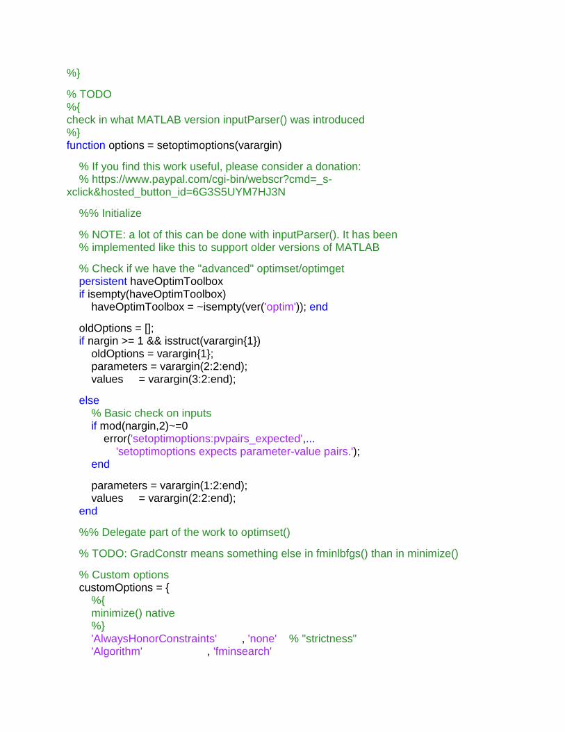
% TODO
%{
check in what MATLAB version inputParser() was introduced
%}
function options = setoptimoptions(varargin)
% If you find this work useful, please consider a donation: % https://www.paypal.com/cgi-bin/webscr?cmd=_s-xclick&hosted_button_id=6G3S5UYM7HJ3N
%% Initialize
% NOTE: a lot of this can be done with inputParser(). It has been % implemented like this to support older versions of MATLAB % Check if we have the "advanced" optimset/optimget persistent haveOptimToolbox
if isempty(haveOptimToolbox)
haveOptimToolbox = ~isempty(ver('optim')); end
oldOptions = []; if nargin >= 1 && isstruct(varargin{1})
oldOptions = varargin{1}; parameters = varargin(2:2:end); values = varargin(3:2:end); else % Basic check on inputs
if mod(nargin,2)~=0
error('setoptimoptions:pvpairs_expected',... 'setoptimoptions expects parameter-value pairs.'); end
parameters = varargin(1:2:end); values = varargin(2:2:end); end
%% Delegate part of the work to optimset()
% TODO: GradConstr means something else in fminlbfgs() than in minimize()
% Custom options
customOptions = {
%{
minimize() native
%}
'AlwaysHonorConstraints' , 'none' % "strictness"
'Algorithm' , 'fminsearch'
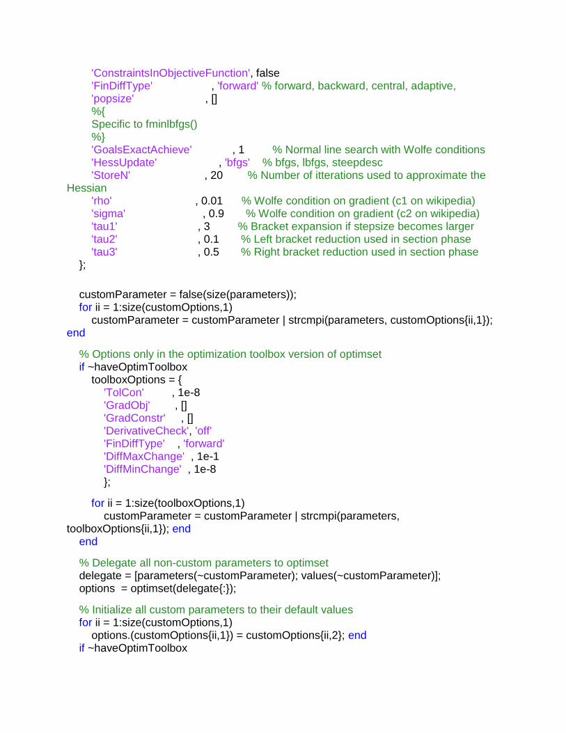
'ConstraintsInObjectiveFunction', false
'FinDiffType' , 'forward' % forward, backward, central, adaptive, 'popsize' , [] %{
Specific to fminlbfgs()
%}
'GoalsExactAchieve' , 1 % Normal line search with Wolfe conditions
'HessUpdate' , 'bfgs' % bfgs, lbfgs, steepdesc
'StoreN' , 20 % Number of itterations used to approximate the Hessian
'rho' , 0.01 % Wolfe condition on gradient (c1 on wikipedia)
'sigma' , 0.9 % Wolfe condition on gradient (c2 on wikipedia)
'tau1' , 3 % Bracket expansion if stepsize becomes larger
'tau2' , 0.1 % Left bracket reduction used in section phase
'tau3' , 0.5 % Right bracket reduction used in section phase
}; customParameter = false(size(parameters)); for ii = 1:size(customOptions,1)
customParameter = customParameter | strcmpi(parameters, customOptions{ii,1}); end
% Options only in the optimization toolbox version of optimset if ~haveOptimToolbox
toolboxOptions = {
'TolCon' , 1e-8
'GradObj' , [] 'GradConstr' , [] 'DerivativeCheck', 'off' 'FinDiffType' , 'forward' 'DiffMaxChange' , 1e-1
'DiffMinChange' , 1e-8
}; for ii = 1:size(toolboxOptions,1)
customParameter = customParameter | strcmpi(parameters, toolboxOptions{ii,1}); end
end
% Delegate all non-custom parameters to optimset delegate = [parameters(~customParameter); values(~customParameter)];
options = optimset(delegate{:}); % Initialize all custom parameters to their default values
for ii = 1:size(customOptions,1)
options.(customOptions{ii,1}) = customOptions{ii,2}; end
if ~haveOptimToolbox

for ii = 1:size(toolboxOptions,1)
options.(toolboxOptions{ii,1}) = toolboxOptions{ii,2}; end
end
% Merge any old options with new ones
if ~isempty(oldOptions)
fOld = fieldnames(oldOptions); % Custom options
for ii = 1:numel(customOptions(:,1))
if ~any(strcmpi(parameters, customOptions{ii,1})) && isfield(oldOptions, customOptions{ii,1}) && ~isempty(oldOptions.(customOptions{ii,1}))
options.(customOptions{ii,1}) = oldOptions.(customOptions{ii,1});
fOld(strcmpi(fOld,customOptions{ii,1})) = []; end
end
% Toolbox options
if ~haveOptimToolbox
for ii = 1:numel(toolboxOptions(:,1))
if ~any(strcmpi(parameters, toolboxOptions{ii,1})) && isfield(oldOptions, toolboxOptions{ii,1}) && ~isempty(oldOptions.(toolboxOptions{ii,1}))
options.(toolboxOptions{ii,1}) = oldOptions.(toolboxOptions{ii,1});
fOld(strcmpi(fOld,toolboxOptions{ii,1})) = []; end
end
end
% All other options
if ~isempty(fOld)
for ii = 1:numel(fOld) if ~any(strcmpi(parameters, fOld{ii})) && isfield(oldOptions, fOld{ii}) && ~isempty(oldOptions.(fOld{ii}))
options.(fOld{ii}) = oldOptions.(fOld{ii}); end
end
end
end
%% Parse the PV-pairs % The remainder
parameters = parameters(customParameter); values = values(customParameter); if ~isempty(parameters)
for ii = 1:numel(parameters)
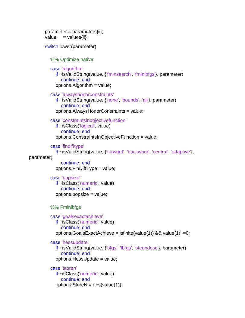
parameter = parameters{ii}; value = values{ii}; switch lower(parameter)
%% Optimize native
case 'algorithm' if ~isValidString(value, {'fminsearch', 'fminlbfgs'}, parameter)
continue; end
options.Algorithm = value; case 'alwayshonorconstraints' if ~isValidString(value, {'none', 'bounds', 'all'}, parameter)
continue; end
options.AlwaysHonorConstraints = value; case 'constraintsinobjectivefunction' if ~isClass('logical', value)
continue; end
options.ConstraintsInObjectiveFunction = value; case 'findifftype' if ~isValidString(value, {'forward', 'backward', 'central', 'adaptive'}, parameter)
continue; end options.FinDiffType = value; case 'popsize' if ~isClass('numeric', value)
continue; end
options.popsize = value; %% Fminlbfgs
case 'goalsexactachieve' if ~isClass('numeric', value)
continue; end
options.GoalsExactAchieve = isfinite(value(1)) && value(1)~=0; case 'hessupdate' if ~isValidString(value, {'bfgs', 'lbfgs', 'steepdesc'}, parameter)
continue; end
options.HessUpdate = value; case 'storen' if ~isClass('numeric', value)
continue; end
options.StoreN = abs(value(1));
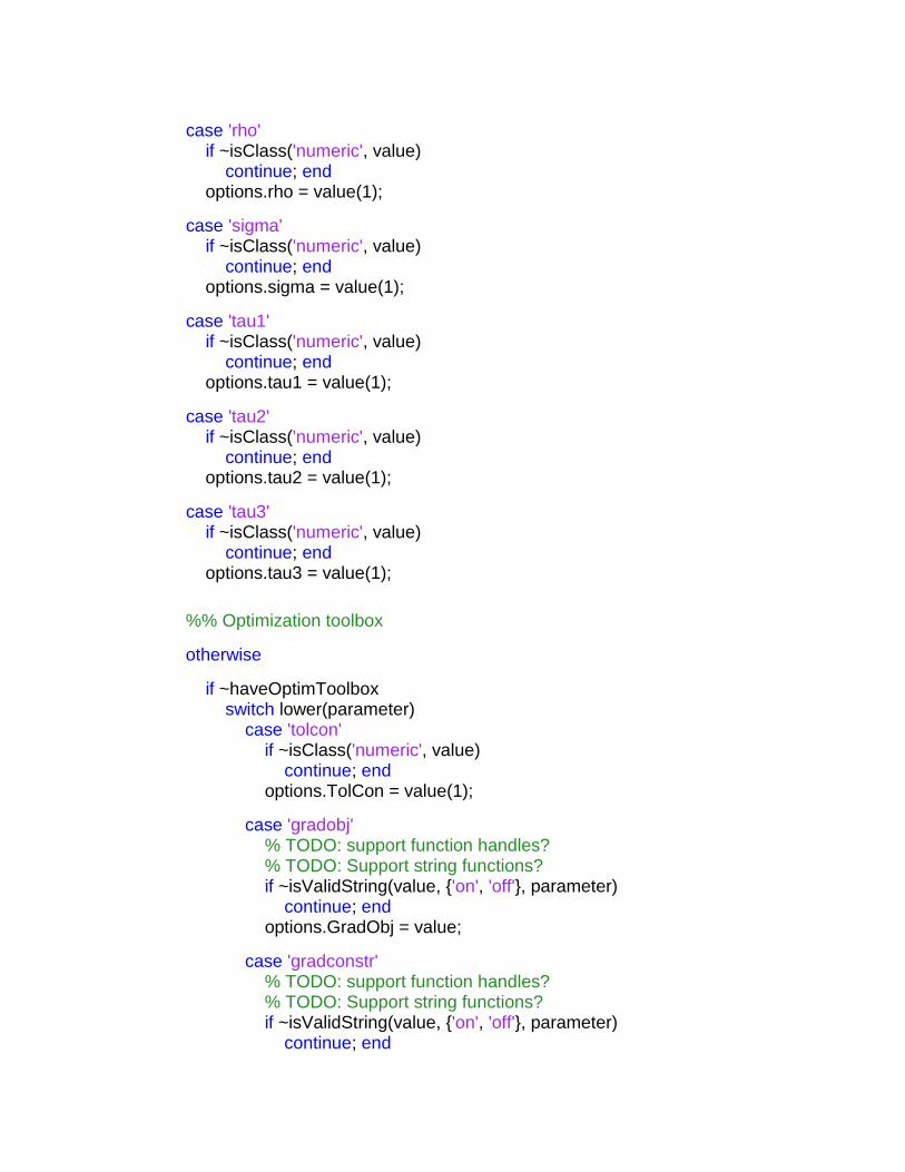
case 'rho' if ~isClass('numeric', value)
continue; end
options.rho = value(1); case 'sigma' if ~isClass('numeric', value)
continue; end
options.sigma = value(1); case 'tau1' if ~isClass('numeric', value)
continue; end
options.tau1 = value(1); case 'tau2' if ~isClass('numeric', value)
continue; end
options.tau2 = value(1); case 'tau3' if ~isClass('numeric', value)
continue; end
options.tau3 = value(1); %% Optimization toolbox
otherwise
if ~haveOptimToolbox
switch lower(parameter)
case 'tolcon' if ~isClass('numeric', value)
continue; end
options.TolCon = value(1); case 'gradobj' % TODO: support function handles?
% TODO: Support string functions?
if ~isValidString(value, {'on', 'off'}, parameter)
continue; end
options.GradObj = value; case 'gradconstr' % TODO: support function handles?
% TODO: Support string functions?
if ~isValidString(value, {'on', 'off'}, parameter)
continue; end
options.GradConstr = value; case 'derivativecheck' if ~isValidString(value, {'yes', 'no'}, parameter)
continue; end
% TODO: valid strings
options.DerivativeCheck = value; case 'findifftype' if ~isValidString(value, {'central', 'forward', 'backward'}, parameter)
continue; end
options.FinDiffType = value; case 'diffmaxchange' if ~isClass('numeric', value)
continue; end
options.DiffMaxChange = value(1); case 'diffminchange' if ~isClass('numeric', value)
continue; end
options.DiffMinChange = value(1); otherwise
warning(... 'setoptimoptions:unknown_option',... 'Unknown option: ''%s''. Ignoring...', parameter); continue
end
else
warning(... 'setoptimoptions:unknown_option',... 'Unknown option: ''%s''. Ignoring...', parameter); continue
end
end % switch
end % for
end % if end % function % Check if given string is one of the supported options. Generate
% appropriate warning messages if this is not the case. % NOTE: this is virtually the same as validatestring(), but this version
% can also be used on older versions of MATLAB function go_on = isValidString(received, validStrings, parameter)
go_on = true; if ~isClass('char', received)
go_on = false; return; end
if ~any(strcmpi(received, validStrings))
validStrings = [ cellfun(@(x) ['''' x ''', '], validStrings(1:end-1), 'UniformOutput', false),... ['and ''' validStrings(end) '''.'] ]; warning(... 'setoptimoptions:unsupported_value',... ['Unsupported option ''%s'' for parameter ''%s''.\n',... 'Valid options are: ' validStrings{:} '\nUsing default...'], ... received, parameter); go_on = false; end
end
% Check if class of given value is correct. Generate appropriate warning
% message if this is not the case. % NOTE: this is virtually the same as validateattributes(), but this % version can also be used on older versions of MATLAB function go_on = isClass(expected, received)
go_on = true; % More than one type may be allowable: if ischar(expected)
isCorrectClass = isa(received, expected); elseif iscell(expected) isCorrectClass = any(cellfun(@(x) isa(received, x), expected));
else
error(... 'setoptimoptions:BUG',... 'An internal error has occurred; please report this to the lead developer.'); end
% Generate warning if the type is not any of the supported ones
if ~isempty(received) && ~isCorrectClass
warning(... 'setoptimoptions:invalid_value',... 'Expected ''%s'', got ''%s''. Ignoring...', expected, class(received)); go_on = false;
end
end
% Check validity of file/function given as strnig
% NOTE: this functionality is deprecated, so a warning is ALWAYS issued. function [go_on, value] = checkFunction(value)
go_on = true; if ischar(value)
warning(... 'setoptimoptions:deprecated',... 'Using string functions or file names of MATLAB functions is deprecated; please use function_handles.'); if ~any(exist(value,'file')==[2 3 5 6])
warning(... 'setoptimoptions:invalid_script',... ['The file/function ''%s'' is invalid, or is not on the MATLAB search path.\n',... 'Using default...'], value); go_on = false; end
% Strip any extension, and convert to valid function handle
value = str2func(regexprep(value, '\.\w*$', '')); end
end
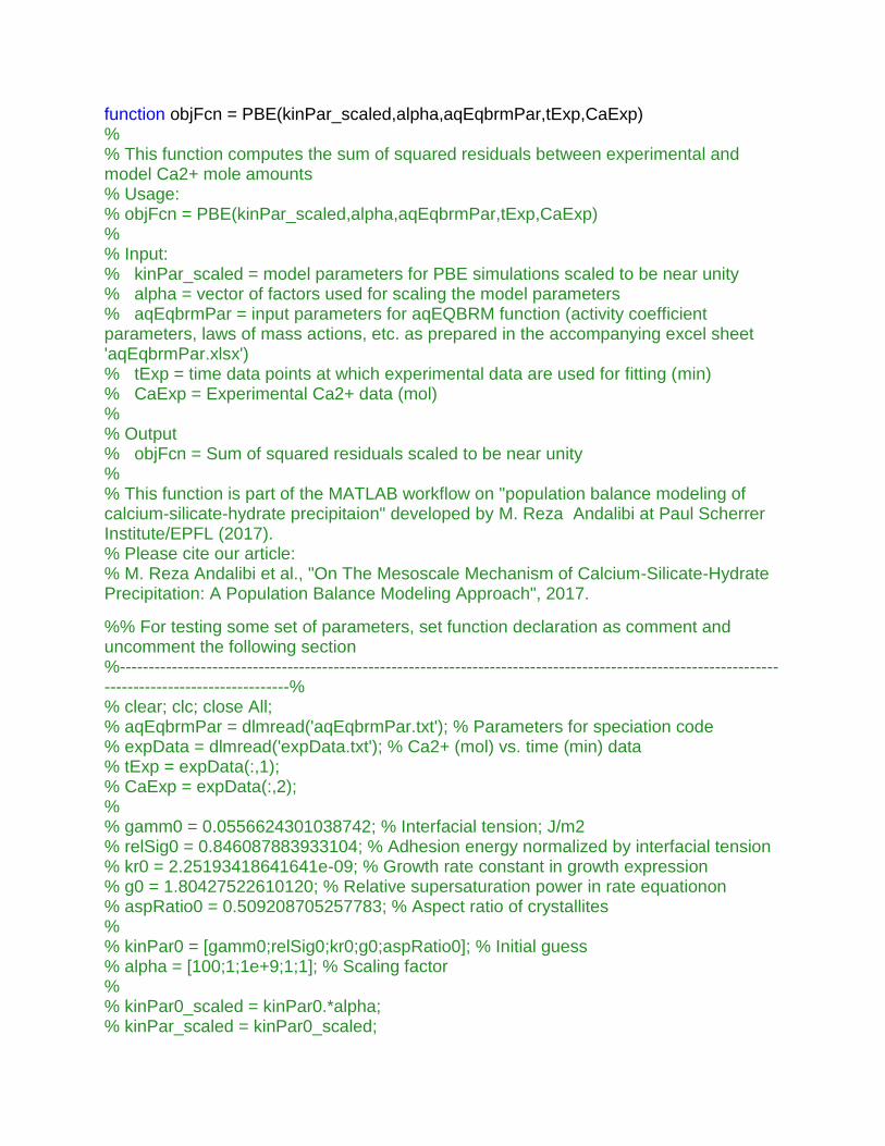
function objFcn = PBE(kinPar_scaled,alpha,aqEqbrmPar,tExp,CaExp)
% % This function computes the sum of squared residuals between experimental and model Ca2+ mole amounts
% Usage: % objFcn = PBE(kinPar_scaled,alpha,aqEqbrmPar,tExp,CaExp)
% % Input: % kinPar_scaled = model parameters for PBE simulations scaled to be near unity
% alpha = vector of factors used for scaling the model parameters
% aqEqbrmPar = input parameters for aqEQBRM function (activity coefficient parameters, laws of mass actions, etc. as prepared in the accompanying excel sheet 'aqEqbrmPar.xlsx')
% tExp = time data points at which experimental data are used for fitting (min)
% CaExp = Experimental Ca2+ data (mol)
% % Output % objFcn = Sum of squared residuals scaled to be near unity
% % This function is part of the MATLAB workflow on "population balance modeling of calcium-silicate-hydrate precipitaion" developed by M. Reza Andalibi at Paul Scherrer Institute/EPFL (2017). % Please cite our article: % M. Reza Andalibi et al., "On The Mesoscale Mechanism of Calcium-Silicate-Hydrate Precipitation: A Population Balance Modeling Approach", 2017. %% For testing some set of parameters, set function declaration as comment and uncomment the following section
%--------------------------------------------------------------------------------------------------------------------------------------------------%
% clear; clc; close All; % aqEqbrmPar = dlmread('aqEqbrmPar.txt'); % Parameters for speciation code
% expData = dlmread('expData.txt'); % Ca2+ (mol) vs. time (min) data
% tExp = expData(:,1); % CaExp = expData(:,2); % % gamm0 = 0.0556624301038742; % Interfacial tension; J/m2
% relSig0 = 0.846087883933104; % Adhesion energy normalized by interfacial tension
% kr0 = 2.25193418641641e-09; % Growth rate constant in growth expression
% g0 = 1.80427522610120; % Relative supersaturation power in rate equationon
% aspRatio0 = 0.509208705257783; % Aspect ratio of crystallites
% % kinPar0 = [gamm0;relSig0;kr0;g0;aspRatio0]; % Initial guess
% alpha = [100;1;1e+9;1;1]; % Scaling factor
% % kinPar0_scaled = kinPar0.*alpha; % kinPar_scaled = kinPar0_scaled;
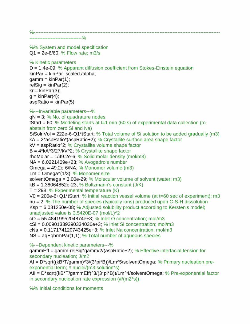
%--------------------------------------------------------------------------------------------------------------------------------------------------%
%% System and model specification
Q1 = 2e-6/60; % Flow rate; m3/s
% Kinetic parameters
D = 1.4e-09; % Apparant diffusion coefficient from Stokes-Einstein equation
kinPar = kinPar_scaled./alpha; gamm = kinPar(1); relSig = kinPar(2); kr = kinPar(3); g = kinPar(4); aspRatio = kinPar(5); %---Invariable parameters---%
qN = 3; % No. of quadrature nodes
tStart = 60; % Modeling starts at t=1 min (60 s) of experimental data collection (to abstain from zero Si and Na)
SiSolnVol = 222e-6-Q1*tStart; % Total volume of Si solution to be added gradually (m3)
kA = 2*aspRatio*(aspRatio+2); % Crystallite surface area shape factor
kV = aspRatio^2; % Crystallite volume shape factor
B = 4*kA^3/27/kV^2; % Crystallite shape factor
rhoMolar = 1/49.2e-6; % Solid molar density (mol/m3)
NA = 6.0221409e+23; % Avogadro's number
Omega = 49.2e-6/NA; % Monomer volume (m3)
Lm = Omega^(1/3); % Monomer size
solventOmega = 3.00e-29; % Molecular volume of solvent (water; m3)
kB = 1.38064852e-23; % Boltzmann's constant (J/K)
T = 298; % Experimental temperature (K)
V0 = 200e-6+Q1*tStart; % Initial reaction vessel volume (at t=60 sec of experiment); m3
nu = 2; % The number of species (typically ions) produced upon C-S-H dissolution
Ksp = 6.031250e-08; % Adjusted solubility product according to Kersten's model; unadjusted value is 3.5420E-07 (mol/L)^2
cO = 55.4841995204874e+3; % Inlet O concentration; mol/m3
cSi = 0.00901339390334036e+3; % Inlet Si concentration; mol/m3
cNa = 0.117174120743425e+3; % Inlet Na concentration; mol/m3
NS = aqEqbrmPar(1,1); % Total number of aqueous species
%---Dependent kinetic parameters---%
gammEff = gamm-relSig*gamm/2/(aspRatio+2); % Effective interfacial tension for secondary nucleation; J/m2
AI = D*sqrt((kB*T/gamm)^3/(3*pi*B))/Lm^5/solventOmega; % Primary nucleation pre-exponential term; # nuclei/(m3 solution*s)
AII = D*sqrt((kB*T/gammEff)^3/(3*pi*B))/Lm^4/solventOmega; % Pre-exponential factor in secondary nucleation rate expression (#/(m2*s))
%% Initial conditions for moments
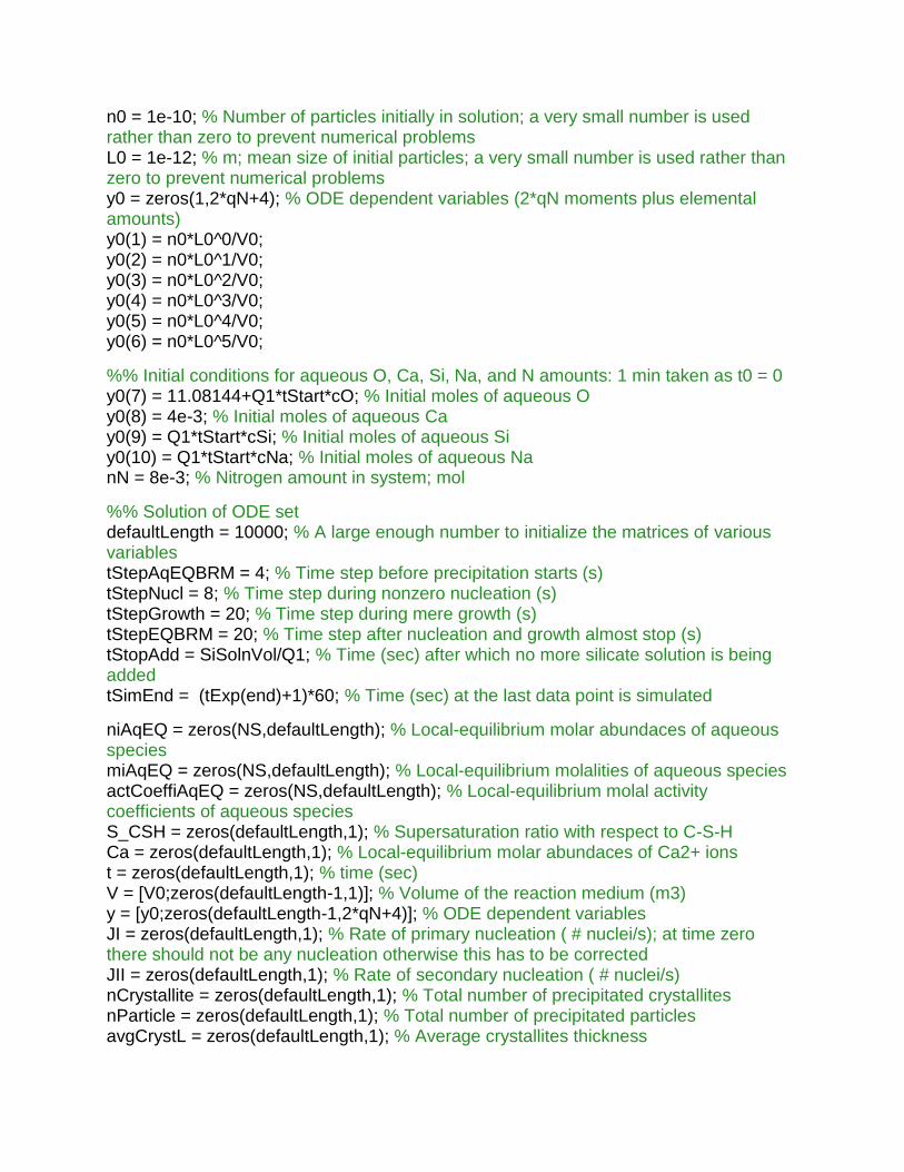
n0 = 1e-10; % Number of particles initially in solution; a very small number is used rather than zero to prevent numerical problems
L0 = 1e-12; % m; mean size of initial particles; a very small number is used rather than zero to prevent numerical problems
y0 = zeros(1,2*qN+4); % ODE dependent variables (2*qN moments plus elemental amounts)
y0(1) = n0*L0^0/V0; y0(2) = n0*L0^1/V0; y0(3) = n0*L0^2/V0; y0(4) = n0*L0^3/V0; y0(5) = n0*L0^4/V0; y0(6) = n0*L0^5/V0; %% Initial conditions for aqueous O, Ca, Si, Na, and N amounts: 1 min taken as t0 = 0
y0(7) = 11.08144+Q1*tStart*cO; % Initial moles of aqueous O
y0(8) = 4e-3; % Initial moles of aqueous Ca
y0(9) = Q1*tStart*cSi; % Initial moles of aqueous Si y0(10) = Q1*tStart*cNa; % Initial moles of aqueous Na
nN = 8e-3; % Nitrogen amount in system; mol %% Solution of ODE set defaultLength = 10000; % A large enough number to initialize the matrices of various variables
tStepAqEQBRM = 4; % Time step before precipitation starts (s)
tStepNucl = 8; % Time step during nonzero nucleation (s)
tStepGrowth = 20; % Time step during mere growth (s)
tStepEQBRM = 20; % Time step after nucleation and growth almost stop (s)
tStopAdd = SiSolnVol/Q1; % Time (sec) after which no more silicate solution is being added
tSimEnd = (tExp(end)+1)*60; % Time (sec) at the last data point is simulated
niAqEQ = zeros(NS,defaultLength); % Local-equilibrium molar abundaces of aqueous species
miAqEQ = zeros(NS,defaultLength); % Local-equilibrium molalities of aqueous species
actCoeffiAqEQ = zeros(NS,defaultLength); % Local-equilibrium molal activity coefficients of aqueous species
S_CSH = zeros(defaultLength,1); % Supersaturation ratio with respect to C-S-H
Ca = zeros(defaultLength,1); % Local-equilibrium molar abundaces of Ca2+ ions
t = zeros(defaultLength,1); % time (sec)
V = [V0;zeros(defaultLength-1,1)]; % Volume of the reaction medium (m3)
y = [y0;zeros(defaultLength-1,2*qN+4)]; % ODE dependent variables
JI = zeros(defaultLength,1); % Rate of primary nucleation ( # nuclei/s); at time zero there should not be any nucleation otherwise this has to be corrected
JII = zeros(defaultLength,1); % Rate of secondary nucleation ( # nuclei/s)
nCrystallite = zeros(defaultLength,1); % Total number of precipitated crystallites
nParticle = zeros(defaultLength,1); % Total number of precipitated particles
avgCrystL = zeros(defaultLength,1); % Average crystallites thickness
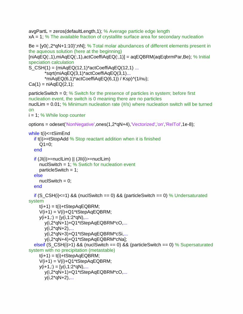
avgPartL = zeros(defaultLength,1); % Average particle edge length
xA = 1; % The available fraction of crystallite surface area for secondary nucleation
Be = [y0(:,2*qN+1:10)';nN]; % Total molar abundances of different elements present in the aqueous solution (here at the beginning)
[niAqEQ(:,1),miAqEQ(:,1),actCoeffiAqEQ(:,1)] = aqEQBRM(aqEqbrmPar,Be); % Initial speciation calculation
S_CSH(1) = (miAqEQ(12,1)*actCoeffiAqEQ(12,1) ... *sqrt(miAqEQ(3,1)*actCoeffiAqEQ(3,1)... *miAqEQ(6,1)*actCoeffiAqEQ(6,1)) / Ksp)^(1/nu); Ca(1) = niAqEQ(2,1); particleSwitch = 0; % Switch for the presence of particles in system; before first nucleation event, the switch is 0 meaning there are no particles
nuclLim = 0.01; % Minimum nucleation rate (#/s) where nucleation switch will be turned on
i = 1; % While loop counter
options = odeset('NonNegative',ones(1,2*qN+4),'Vectorized','on','RelTol',1e-8); while t(i)<=tSimEnd
if t(i)>=tStopAdd % Stop reactant addition when it is finished
Q1=0; end
if (JI(i)>=nuclLim) || (JII(i)>=nuclLim)
nuclSwitch = 1; % Swtich for nucleation event particleSwitch = 1; else
nuclSwitch = 0; end
if (S_CSH(i)<=1) && (nuclSwitch == 0) && (particleSwitch == 0) % Undersaturated system
t(i+1) = t(i)+tStepAqEQBRM; V(i+1) = V(i)+Q1*tStepAqEQBRM; y(i+1,:) = [y(i,1:2*qN),... y(i,2*qN+1)+Q1*tStepAqEQBRM*cO,... y(i,2*qN+2),... y(i,2*qN+3)+Q1*tStepAqEQBRM*cSi,... y(i,2*qN+4)+Q1*tStepAqEQBRM*cNa]; elseif (S_CSH(i)>1) && (nuclSwitch == 0) && (particleSwitch == 0) % Supersaturated system with no precipitation (metastable)
t(i+1) = t(i)+tStepAqEQBRM; V(i+1) = V(i)+Q1*tStepAqEQBRM; y(i+1,:) = [y(i,1:2*qN),... y(i,2*qN+1)+Q1*tStepAqEQBRM*cO,... y(i,2*qN+2),...
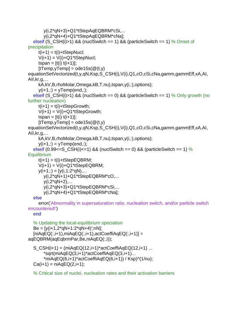
y(i,2*qN+3)+Q1*tStepAqEQBRM*cSi,... y(i,2*qN+4)+Q1*tStepAqEQBRM*cNa]; elseif (S_CSH(i)>1) && (nuclSwitch == 1) && (particleSwitch == 1) % Onset of precipitation
t(i+1) = t(i)+tStepNucl; V(i+1) = V(i)+Q1*tStepNucl; tspan = [t(i) t(i+1)]; [tTemp,yTemp] = ode15s(@(t,y) equationSetVectorized(t,y,qN,Ksp,S_CSH(i),V(i),Q1,cO,cSi,cNa,gamm,gammEff,xA,AI,AII,kr,g,... kA,kV,B,rhoMolar,Omega,kB,T,nu),tspan,y(i,:),options); y(i+1,:) = yTemp(end,:); elseif (S_CSH(i)>1) && (nuclSwitch == 0) && (particleSwitch == 1) % Only growth (no further nucleation)
t(i+1) = t(i)+tStepGrowth; V(i+1) = V(i)+Q1*tStepGrowth; tspan = [t(i) t(i+1)]; [tTemp,yTemp] = ode15s(@(t,y) equationSetVectorized(t,y,qN,Ksp,S_CSH(i),V(i),Q1,cO,cSi,cNa,gamm,gammEff,xA,AI,AII,kr,g,... kA,kV,B,rhoMolar,Omega,kB,T,nu),tspan,y(i,:),options); y(i+1,:) = yTemp(end,:); elseif (0.99<=S_CSH(i)<=1) && (nuclSwitch == 0) && (particleSwitch == 1) % Equilibrium
t(i+1) = t(i)+tStepEQBRM; V(i+1) = V(i)+Q1*tStepEQBRM; y(i+1,:) = [y(i,1:2*qN),... y(i,2*qN+1)+Q1*tStepEQBRM*cO,... y(i,2*qN+2),... y(i,2*qN+3)+Q1*tStepEQBRM*cSi,... y(i,2*qN+4)+Q1*tStepEQBRM*cNa]; else
error('Abnormality in supersaturation ratio, nucleation switch, and/or particle switch encountered!')
end
% Updating the local-equilibrium speciation
Be = [y(i+1,2*qN+1:2*qN+4)';nN]; [niAqEQ(:,i+1),miAqEQ(:,i+1),actCoeffiAqEQ(:,i+1)] = aqEQBRM(aqEqbrmPar,Be,niAqEQ(:,i)); S_CSH(i+1) = (miAqEQ(12,i+1)*actCoeffiAqEQ(12,i+1) ... *sqrt(miAqEQ(3,i+1)*actCoeffiAqEQ(3,i+1)... *miAqEQ(6,i+1)*actCoeffiAqEQ(6,i+1)) / Ksp)^(1/nu); Ca(i+1) = niAqEQ(2,i+1); % Critical size of nuclei, nucleation rates and their activation barriers
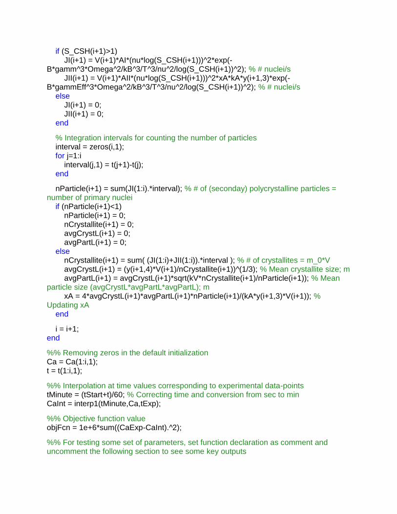
if (S_CSH(i+1)>1)
JI(i+1) = V(i+1)*AI*(nu*log(S_CSH(i+1)))^2*exp(-B*gamm^3*Omega^2/kB^3/T^3/nu^2/log(S_CSH(i+1))^2); % # nuclei/s
JII(i+1) = V(i+1)*AII*(nu*log(S_CSH(i+1)))^2*xA*kA*y(i+1,3)*exp(-B*gammEff^3*Omega^2/kB^3/T^3/nu^2/log(S_CSH(i+1))^2); % # nuclei/s
else
JI(i+1) = 0; JII(i+1) = 0; end
% Integration intervals for counting the number of particles
interval = zeros(i,1); for j=1:i interval(j,1) = t(j+1)-t(j); end
nParticle(i+1) = sum(JI(1:i).*interval); % # of (seconday) polycrystalline particles = number of primary nuclei if (nParticle(i+1)<1)
nParticle(i+1) = 0; nCrystallite(i+1) = 0; avgCrystL(i+1) = 0; avgPartL(i+1) = 0; else
nCrystallite(i+1) = sum( (JI(1:i)+JII(1:i)).*interval ); % # of crystallites = m_0*V
avgCrystL(i+1) = (y(i+1,4)*V(i+1)/nCrystallite(i+1))^(1/3); % Mean crystallite size; m
avgPartL(i+1) = avgCrystL(i+1)*sqrt(kV*nCrystallite(i+1)/nParticle(i+1)); % Mean particle size (avgCrystL*avgPartL*avgPartL); m
xA = 4*avgCrystL(i+1)*avgPartL(i+1)*nParticle(i+1)/(kA*y(i+1,3)*V(i+1)); % Updating xA
end
i = i+1; end
%% Removing zeros in the default initialization
Ca = Ca(1:i,1); t = t(1:i,1); %% Interpolation at time values corresponding to experimental data-points
tMinute = (tStart+t)/60; % Correcting time and conversion from sec to min
CaInt = interp1(tMinute,Ca,tExp); %% Objective function value
objFcn = 1e+6*sum((CaExp-CaInt).^2); %% For testing some set of parameters, set function declaration as comment and uncomment the following section to see some key outputs

%--------------------------------------------------------------------------------------------------------------------------------------------------%
% fig = fig('Name','Fitted Ca2+ mole amounts','Color','white'); % ax = axes('Parent',fig); % plot(tExp,CaExp,'bo','MarkerSize',5); hold on; % plot(tExp,CaInt,'r-','LineWidth',2); % set(ax,'FontSize',22,'FontWeight','bold'); % % axis square
% xlabel('Time (min)')
% ylabel('Aqueous Ca2+ amount (mol)')
% hold off % avgCrystL = 1e+9*avgCrystL(1:i,1); % nm
% avgPartL = 1e+9*avgPartL(1:i,1); % nm
% avgCrystL(end)
% avgPartL(end)
% S_Port = sqrt( (miAqEQ(2,:).*actCoeffiAqEQ(2,:).*(miAqEQ(6,:).*actCoeffiAqEQ(6,:)).^2)/3.85080e-6 ); % max(S_Port)
%--------------------------------------------------------------------------------------------------------------------------------------------------%

function dydt = equationSetVectorized(t,y,qN,Ksp,S,V,Q1,cO,cSi,cNa,gamm,gammEff,xA,AI,AII,kr,g,avgCrystL,... kA,kV,B,rhoMolar,Omega,kB,T,nu)
% % This function generates the set of ODEs (PBE + mass balances) to be numerically solved for computational modeling of C-S-H precipitation % % Usage: % dydt = equationSetVectorized(t,y,qN,Ksp,S,V,Q1,cO,cSi,cNa,gamm,gammEff,xA,AI,AII,kr,g,avgCrystL,kA,kV,B,rhoMolar,Omega,kB,T,nu) % % Input: % t = Time; % y = Dependent variables (moments + elemental abundances)
% qN = No. of quadrature nodes
% Ksp = Adjusted solubility product according to Kersten's model; unadjusted value is 3.5420E-07 (mol/L)^2
% S = Supersaturation ratio
% V = System volume
% Q1 = Reactant flow rate
% cO = Inlet O concentration; mol/m3
% cSi = Inlet Si concentration; mol/m3
% cNa = Inlet Na concentration; mol/m3
% gamm = Interfacial tension
% gammEff = Effective interfacial tension for secondary nucleation
% xA = The available fraction of crystallite surface area for secondary nucleation
% AI = Primary nucleation pre-exponential term
% AII = Secondary nucleation pre-exponential term
% kr = Growth rate constant in growth expression
% g = Relative supersaturation power in rate equationon
% avgCrystL = Average crystallites thickness
% kA = Surface area shape factor
% kV = Volume shape factor
% B = Shape factor
% rhoMolar = Solid molar density
% Omega = Monomer volume
% kB = Boltzmann's constant % T = Temperature
% nu = The number of species produced upon C-S-H dissolution
% % Output: % dydt = ODE describing the respective dependent variable written in a vectorized manner
%
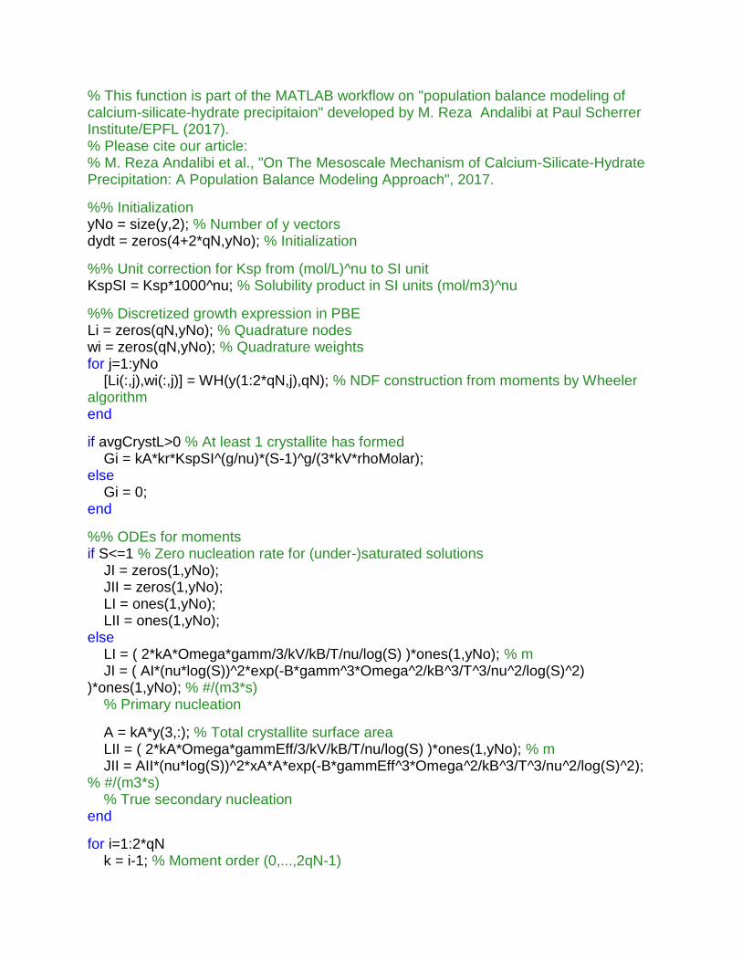
% This function is part of the MATLAB workflow on "population balance modeling of calcium-silicate-hydrate precipitaion" developed by M. Reza Andalibi at Paul Scherrer Institute/EPFL (2017). % Please cite our article: % M. Reza Andalibi et al., "On The Mesoscale Mechanism of Calcium-Silicate-Hydrate Precipitation: A Population Balance Modeling Approach", 2017. %% Initialization
yNo = size(y,2); % Number of y vectors
dydt = zeros(4+2*qN,yNo); % Initialization
%% Unit correction for Ksp from (mol/L)^nu to SI unit KspSI = Ksp*1000^nu; % Solubility product in SI units (mol/m3)^nu
%% Discretized growth expression in PBE
Li = zeros(qN,yNo); % Quadrature nodes
wi = zeros(qN,yNo); % Quadrature weights
for j=1:yNo
[Li(:,j),wi(:,j)] = WH(y(1:2*qN,j),qN); % NDF construction from moments by Wheeler algorithm
end
if avgCrystL>0 % At least 1 crystallite has formed
Gi = kA*kr*KspSI^(g/nu)*(S-1)^g/(3*kV*rhoMolar); else
Gi = 0; end
%% ODEs for moments
if S<=1 % Zero nucleation rate for (under-)saturated solutions
JI = zeros(1,yNo); JII = zeros(1,yNo); LI = ones(1,yNo); LII = ones(1,yNo); else
LI = ( 2*kA*Omega*gamm/3/kV/kB/T/nu/log(S) )*ones(1,yNo); % m
JI = ( AI*(nu*log(S))^2*exp(-B*gamm^3*Omega^2/kB^3/T^3/nu^2/log(S)^2) )*ones(1,yNo); % #/(m3*s)
% Primary nucleation
A = kA*y(3,:); % Total crystallite surface area
LII = ( 2*kA*Omega*gammEff/3/kV/kB/T/nu/log(S) )*ones(1,yNo); % m
JII = AII*(nu*log(S))^2*xA*A*exp(-B*gammEff^3*Omega^2/kB^3/T^3/nu^2/log(S)^2); % #/(m3*s)
% True secondary nucleation
end
for i=1:2*qN
k = i-1; % Moment order (0,...,2qN-1)

dydt(i,:) = -y(i,:)*Q1/V + k*sum(wi.*Gi.*Li.^(k-1),1) + JI.*LI.^k + JII.*LII.^k; end
%% ODEs for mass balances (O(aq), Ca(aq), Si(aq), and Na(aq), respectively)
dCSHdt = (3*sum((wi.*Gi.*Li.^2),1) + JI.*LI.^3 + JII.*LII.^3)*kV*V*rhoMolar; % Rate of CSH precipitation (mol/s)
dydt(2*qN+1,:) = Q1*cO-3.5*dCSHdt; % O
dydt(2*qN+2,:) = -dCSHdt; % Ca
dydt(2*qN+3,:) = Q1*cSi-0.5*dCSHdt; % Si dydt(2*qN+4,:) = Q1*cNa; % Na
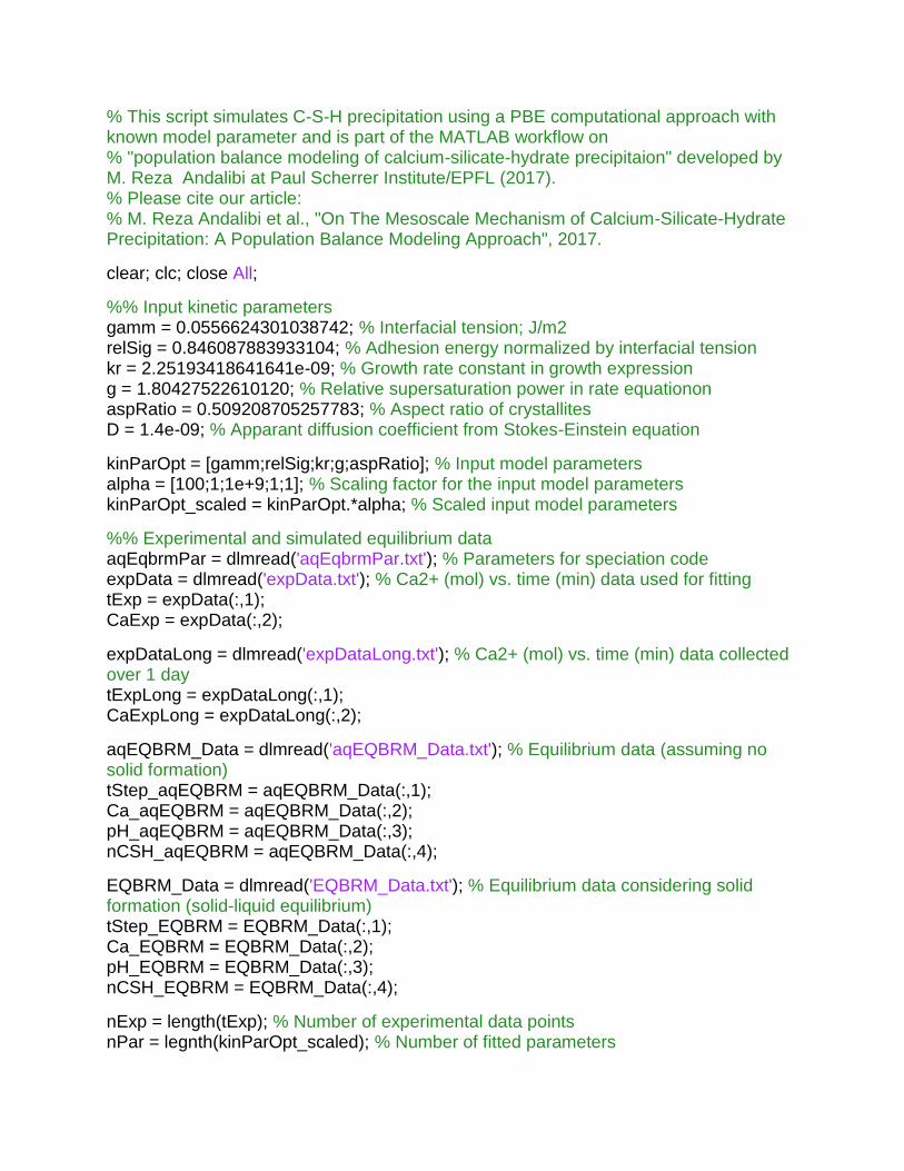
% This script simulates C-S-H precipitation using a PBE computational approach with known model parameter and is part of the MATLAB workflow on
% "population balance modeling of calcium-silicate-hydrate precipitaion" developed by M. Reza Andalibi at Paul Scherrer Institute/EPFL (2017). % Please cite our article: % M. Reza Andalibi et al., "On The Mesoscale Mechanism of Calcium-Silicate-Hydrate Precipitation: A Population Balance Modeling Approach", 2017. clear; clc; close All; %% Input kinetic parameters
gamm = 0.0556624301038742; % Interfacial tension; J/m2
relSig = 0.846087883933104; % Adhesion energy normalized by interfacial tension
kr = 2.25193418641641e-09; % Growth rate constant in growth expression
g = 1.80427522610120; % Relative supersaturation power in rate equationon
aspRatio = 0.509208705257783; % Aspect ratio of crystallites
D = 1.4e-09; % Apparant diffusion coefficient from Stokes-Einstein equation
kinParOpt = [gamm;relSig;kr;g;aspRatio]; % Input model parameters
alpha = [100;1;1e+9;1;1]; % Scaling factor for the input model parameters
kinParOpt_scaled = kinParOpt.*alpha; % Scaled input model parameters
%% Experimental and simulated equilibrium data
aqEqbrmPar = dlmread('aqEqbrmPar.txt'); % Parameters for speciation code
expData = dlmread('expData.txt'); % Ca2+ (mol) vs. time (min) data used for fitting
tExp = expData(:,1); CaExp = expData(:,2); expDataLong = dlmread('expDataLong.txt'); % Ca2+ (mol) vs. time (min) data collected over 1 day
tExpLong = expDataLong(:,1); CaExpLong = expDataLong(:,2); aqEQBRM_Data = dlmread('aqEQBRM_Data.txt'); % Equilibrium data (assuming no solid formation)
tStep_aqEQBRM = aqEQBRM_Data(:,1); Ca_aqEQBRM = aqEQBRM_Data(:,2); pH_aqEQBRM = aqEQBRM_Data(:,3); nCSH_aqEQBRM = aqEQBRM_Data(:,4); EQBRM_Data = dlmread('EQBRM_Data.txt'); % Equilibrium data considering solid formation (solid-liquid equilibrium)
tStep_EQBRM = EQBRM_Data(:,1); Ca_EQBRM = EQBRM_Data(:,2); pH_EQBRM = EQBRM_Data(:,3); nCSH_EQBRM = EQBRM_Data(:,4); nExp = length(tExp); % Number of experimental data points
nPar = legnth(kinParOpt_scaled); % Number of fitted parameters
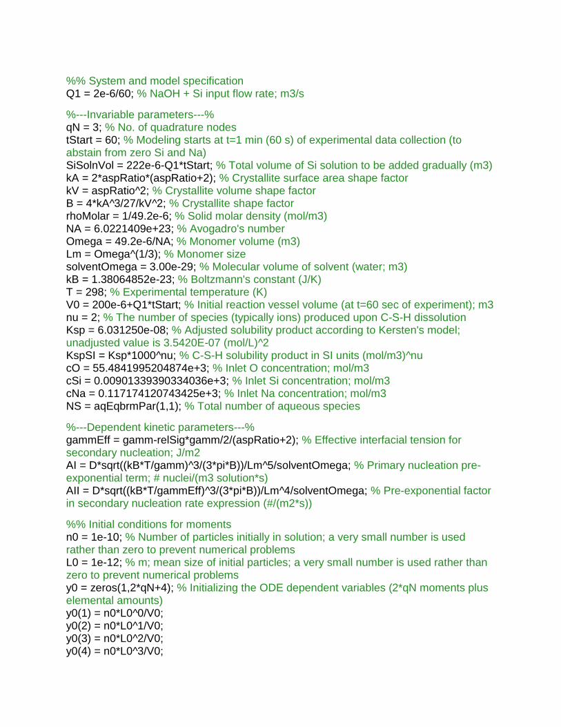
%% System and model specification
Q1 = 2e-6/60; % NaOH + Si input flow rate; m3/s
%---Invariable parameters---%
qN = 3; % No. of quadrature nodes
tStart = 60; % Modeling starts at t=1 min (60 s) of experimental data collection (to abstain from zero Si and Na)
SiSolnVol = 222e-6-Q1*tStart; % Total volume of Si solution to be added gradually (m3)
kA = 2*aspRatio*(aspRatio+2); % Crystallite surface area shape factor
kV = aspRatio^2; % Crystallite volume shape factor
B = 4*kA^3/27/kV^2; % Crystallite shape factor
rhoMolar = 1/49.2e-6; % Solid molar density (mol/m3)
NA = 6.0221409e+23; % Avogadro's number
Omega = 49.2e-6/NA; % Monomer volume (m3)
Lm = Omega^(1/3); % Monomer size
solventOmega = 3.00e-29; % Molecular volume of solvent (water; m3)
kB = 1.38064852e-23; % Boltzmann's constant (J/K)
T = 298; % Experimental temperature (K)
V0 = 200e-6+Q1*tStart; % Initial reaction vessel volume (at t=60 sec of experiment); m3
nu = 2; % The number of species (typically ions) produced upon C-S-H dissolution
Ksp = 6.031250e-08; % Adjusted solubility product according to Kersten's model; unadjusted value is 3.5420E-07 (mol/L)^2
KspSI = Ksp*1000^nu; % C-S-H solubility product in SI units (mol/m3)^nu
cO = 55.4841995204874e+3; % Inlet O concentration; mol/m3
cSi = 0.00901339390334036e+3; % Inlet Si concentration; mol/m3
cNa = 0.117174120743425e+3; % Inlet Na concentration; mol/m3
NS = aqEqbrmPar(1,1); % Total number of aqueous species
%---Dependent kinetic parameters---%
gammEff = gamm-relSig*gamm/2/(aspRatio+2); % Effective interfacial tension for secondary nucleation; J/m2
AI = D*sqrt((kB*T/gamm)^3/(3*pi*B))/Lm^5/solventOmega; % Primary nucleation pre-exponential term; # nuclei/(m3 solution*s)
AII = D*sqrt((kB*T/gammEff)^3/(3*pi*B))/Lm^4/solventOmega; % Pre-exponential factor in secondary nucleation rate expression (#/(m2*s))
%% Initial conditions for moments
n0 = 1e-10; % Number of particles initially in solution; a very small number is used rather than zero to prevent numerical problems
L0 = 1e-12; % m; mean size of initial particles; a very small number is used rather than zero to prevent numerical problems
y0 = zeros(1,2*qN+4); % Initializing the ODE dependent variables (2*qN moments plus elemental amounts)
y0(1) = n0*L0^0/V0; y0(2) = n0*L0^1/V0; y0(3) = n0*L0^2/V0; y0(4) = n0*L0^3/V0;
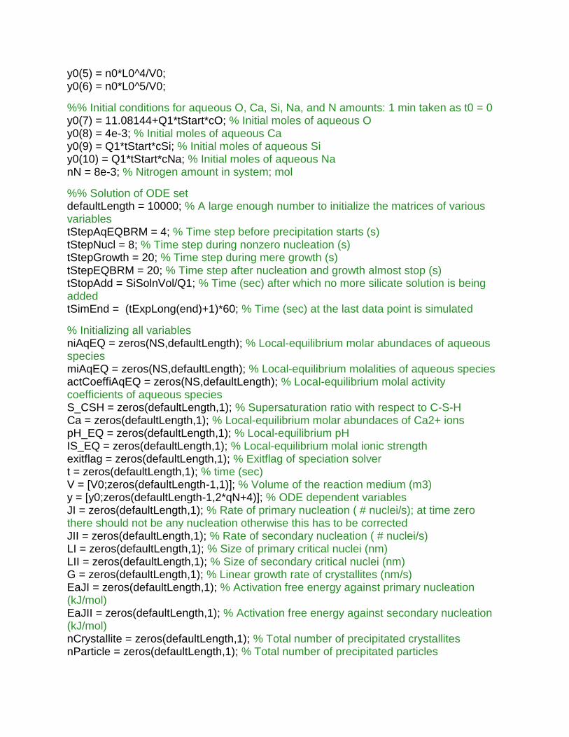
y0(5) = n0*L0^4/V0; y0(6) = n0*L0^5/V0; %% Initial conditions for aqueous O, Ca, Si, Na, and N amounts: 1 min taken as t0 = 0
y0(7) = 11.08144+Q1*tStart*cO; % Initial moles of aqueous O
y0(8) = 4e-3; % Initial moles of aqueous Ca
y0(9) = Q1*tStart*cSi; % Initial moles of aqueous Si y0(10) = Q1*tStart*cNa; % Initial moles of aqueous Na
nN = 8e-3; % Nitrogen amount in system; mol %% Solution of ODE set defaultLength = 10000; % A large enough number to initialize the matrices of various variables
tStepAqEQBRM = 4; % Time step before precipitation starts (s)
tStepNucl = 8; % Time step during nonzero nucleation (s)
tStepGrowth = 20; % Time step during mere growth (s)
tStepEQBRM = 20; % Time step after nucleation and growth almost stop (s)
tStopAdd = SiSolnVol/Q1; % Time (sec) after which no more silicate solution is being added
tSimEnd = (tExpLong(end)+1)*60; % Time (sec) at the last data point is simulated
% Initializing all variables
niAqEQ = zeros(NS,defaultLength); % Local-equilibrium molar abundaces of aqueous species
miAqEQ = zeros(NS,defaultLength); % Local-equilibrium molalities of aqueous species
actCoeffiAqEQ = zeros(NS,defaultLength); % Local-equilibrium molal activity coefficients of aqueous species
S_CSH = zeros(defaultLength,1); % Supersaturation ratio with respect to C-S-H
Ca = zeros(defaultLength,1); % Local-equilibrium molar abundaces of Ca2+ ions
pH_EQ = zeros(defaultLength,1); % Local-equilibrium pH
IS_EQ = zeros(defaultLength,1); % Local-equilibrium molal ionic strength
exitflag = zeros(defaultLength,1); % Exitflag of speciation solver
t = zeros(defaultLength,1); % time (sec)
V = [V0;zeros(defaultLength-1,1)]; % Volume of the reaction medium (m3)
y = [y0;zeros(defaultLength-1,2*qN+4)]; % ODE dependent variables
JI = zeros(defaultLength,1); % Rate of primary nucleation ( # nuclei/s); at time zero there should not be any nucleation otherwise this has to be corrected
JII = zeros(defaultLength,1); % Rate of secondary nucleation ( # nuclei/s)
LI = zeros(defaultLength,1); % Size of primary critical nuclei (nm)
LII = zeros(defaultLength,1); % Size of secondary critical nuclei (nm)
G = zeros(defaultLength,1); % Linear growth rate of crystallites (nm/s)
EaJI = zeros(defaultLength,1); % Activation free energy against primary nucleation (kJ/mol)
EaJII = zeros(defaultLength,1); % Activation free energy against secondary nucleation (kJ/mol)
nCrystallite = zeros(defaultLength,1); % Total number of precipitated crystallites
nParticle = zeros(defaultLength,1); % Total number of precipitated particles
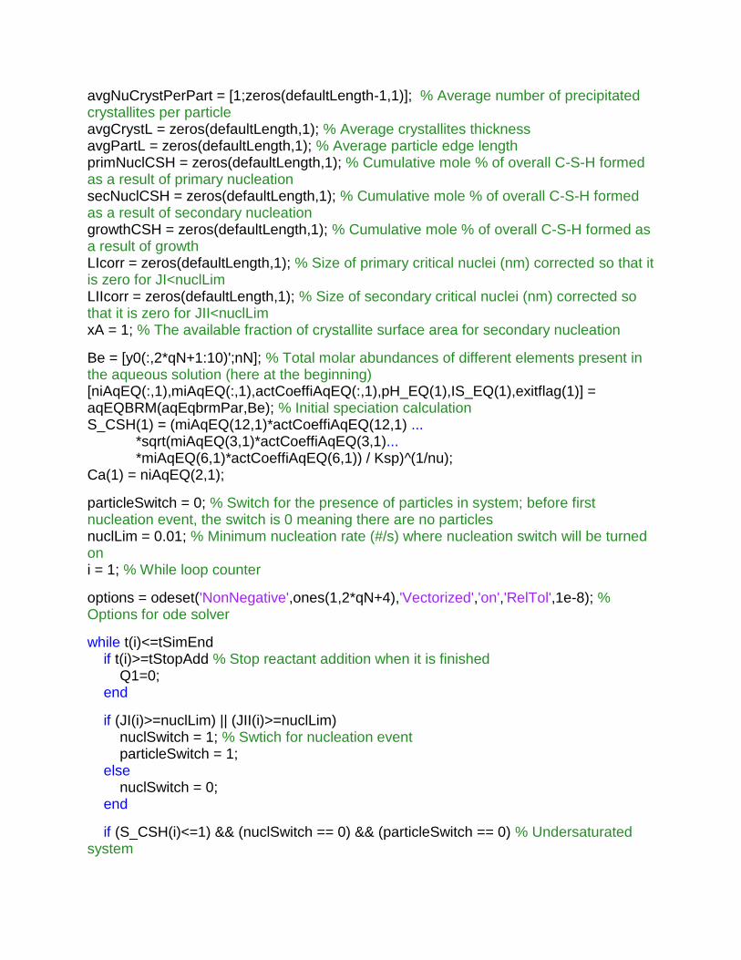
avgNuCrystPerPart = [1;zeros(defaultLength-1,1)]; % Average number of precipitated crystallites per particle
avgCrystL = zeros(defaultLength,1); % Average crystallites thickness
avgPartL = zeros(defaultLength,1); % Average particle edge length
primNuclCSH = zeros(defaultLength,1); % Cumulative mole % of overall C-S-H formed as a result of primary nucleation
secNuclCSH = zeros(defaultLength,1); % Cumulative mole % of overall C-S-H formed as a result of secondary nucleation
growthCSH = zeros(defaultLength,1); % Cumulative mole % of overall C-S-H formed as a result of growth
LIcorr = zeros(defaultLength,1); % Size of primary critical nuclei (nm) corrected so that it is zero for JI<nuclLim
LIIcorr = zeros(defaultLength,1); % Size of secondary critical nuclei (nm) corrected so that it is zero for JII<nuclLim
xA = 1; % The available fraction of crystallite surface area for secondary nucleation
Be = [y0(:,2*qN+1:10)';nN]; % Total molar abundances of different elements present in the aqueous solution (here at the beginning)
[niAqEQ(:,1),miAqEQ(:,1),actCoeffiAqEQ(:,1),pH_EQ(1),IS_EQ(1),exitflag(1)] = aqEQBRM(aqEqbrmPar,Be); % Initial speciation calculation
S_CSH(1) = (miAqEQ(12,1)*actCoeffiAqEQ(12,1) ... *sqrt(miAqEQ(3,1)*actCoeffiAqEQ(3,1)... *miAqEQ(6,1)*actCoeffiAqEQ(6,1)) / Ksp)^(1/nu); Ca(1) = niAqEQ(2,1); particleSwitch = 0; % Switch for the presence of particles in system; before first nucleation event, the switch is 0 meaning there are no particles
nuclLim = 0.01; % Minimum nucleation rate (#/s) where nucleation switch will be turned on
i = 1; % While loop counter
options = odeset('NonNegative',ones(1,2*qN+4),'Vectorized','on','RelTol',1e-8); % Options for ode solver
while t(i)<=tSimEnd
if t(i)>=tStopAdd % Stop reactant addition when it is finished
Q1=0; end
if (JI(i)>=nuclLim) || (JII(i)>=nuclLim)
nuclSwitch = 1; % Swtich for nucleation event particleSwitch = 1; else
nuclSwitch = 0; end
if (S_CSH(i)<=1) && (nuclSwitch == 0) && (particleSwitch == 0) % Undersaturated system
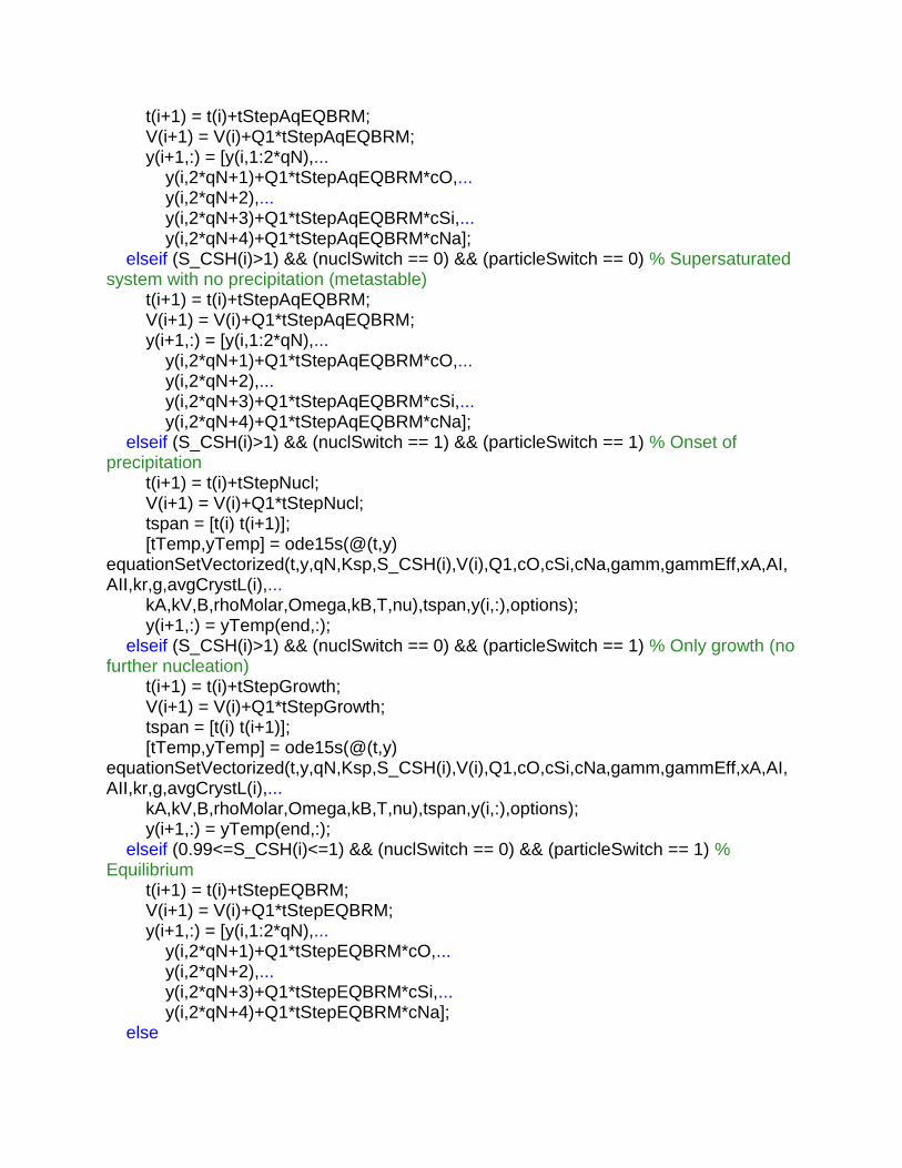
t(i+1) = t(i)+tStepAqEQBRM; V(i+1) = V(i)+Q1*tStepAqEQBRM; y(i+1,:) = [y(i,1:2*qN),... y(i,2*qN+1)+Q1*tStepAqEQBRM*cO,... y(i,2*qN+2),... y(i,2*qN+3)+Q1*tStepAqEQBRM*cSi,... y(i,2*qN+4)+Q1*tStepAqEQBRM*cNa]; elseif (S_CSH(i)>1) && (nuclSwitch == 0) && (particleSwitch == 0) % Supersaturated system with no precipitation (metastable)
t(i+1) = t(i)+tStepAqEQBRM; V(i+1) = V(i)+Q1*tStepAqEQBRM; y(i+1,:) = [y(i,1:2*qN),... y(i,2*qN+1)+Q1*tStepAqEQBRM*cO,... y(i,2*qN+2),... y(i,2*qN+3)+Q1*tStepAqEQBRM*cSi,... y(i,2*qN+4)+Q1*tStepAqEQBRM*cNa]; elseif (S_CSH(i)>1) && (nuclSwitch == 1) && (particleSwitch == 1) % Onset of precipitation
t(i+1) = t(i)+tStepNucl; V(i+1) = V(i)+Q1*tStepNucl; tspan = [t(i) t(i+1)]; [tTemp,yTemp] = ode15s(@(t,y) equationSetVectorized(t,y,qN,Ksp,S_CSH(i),V(i),Q1,cO,cSi,cNa,gamm,gammEff,xA,AI,AII,kr,g,avgCrystL(i),... kA,kV,B,rhoMolar,Omega,kB,T,nu),tspan,y(i,:),options); y(i+1,:) = yTemp(end,:); elseif (S_CSH(i)>1) && (nuclSwitch == 0) && (particleSwitch == 1) % Only growth (no further nucleation)
t(i+1) = t(i)+tStepGrowth; V(i+1) = V(i)+Q1*tStepGrowth; tspan = [t(i) t(i+1)]; [tTemp,yTemp] = ode15s(@(t,y) equationSetVectorized(t,y,qN,Ksp,S_CSH(i),V(i),Q1,cO,cSi,cNa,gamm,gammEff,xA,AI,AII,kr,g,avgCrystL(i),... kA,kV,B,rhoMolar,Omega,kB,T,nu),tspan,y(i,:),options); y(i+1,:) = yTemp(end,:); elseif (0.99<=S_CSH(i)<=1) && (nuclSwitch == 0) && (particleSwitch == 1) % Equilibrium
t(i+1) = t(i)+tStepEQBRM; V(i+1) = V(i)+Q1*tStepEQBRM; y(i+1,:) = [y(i,1:2*qN),... y(i,2*qN+1)+Q1*tStepEQBRM*cO,... y(i,2*qN+2),... y(i,2*qN+3)+Q1*tStepEQBRM*cSi,... y(i,2*qN+4)+Q1*tStepEQBRM*cNa]; else
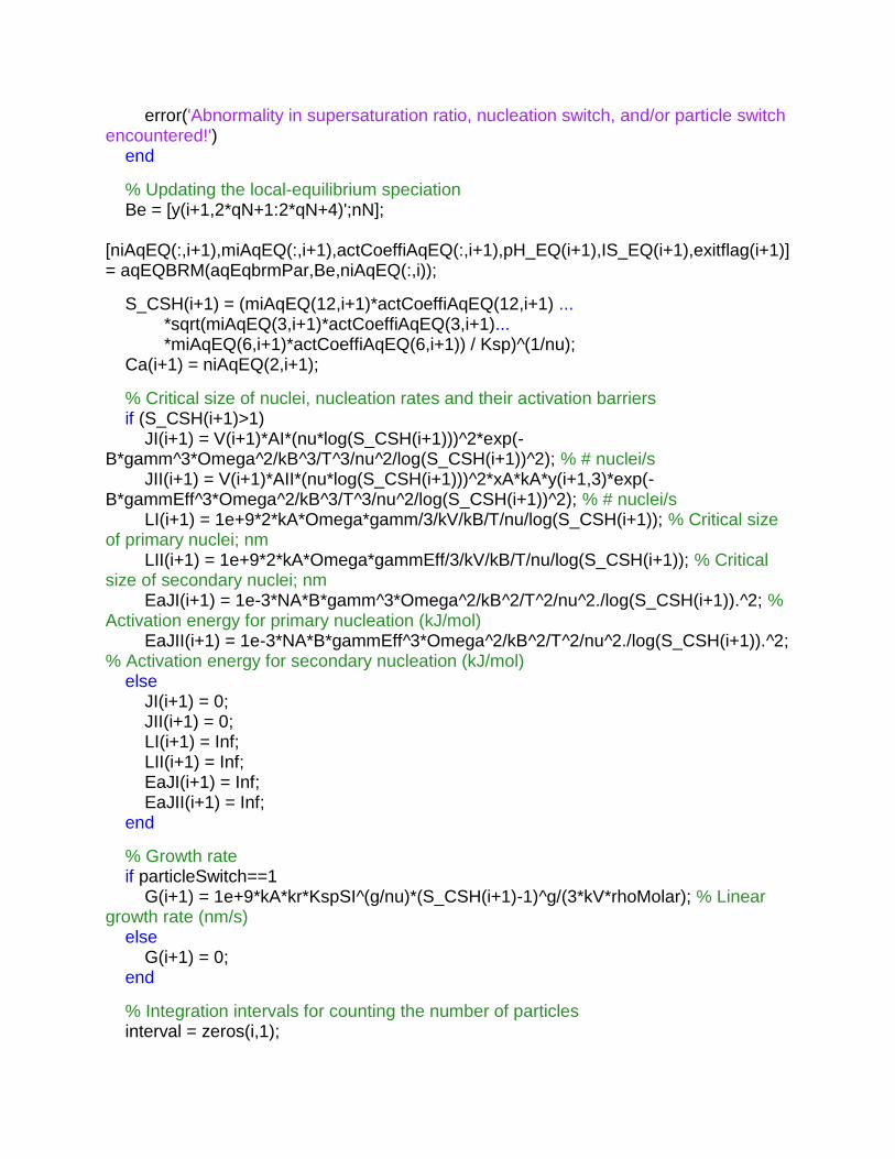
error('Abnormality in supersaturation ratio, nucleation switch, and/or particle switch encountered!')
end
% Updating the local-equilibrium speciation
Be = [y(i+1,2*qN+1:2*qN+4)';nN]; [niAqEQ(:,i+1),miAqEQ(:,i+1),actCoeffiAqEQ(:,i+1),pH_EQ(i+1),IS_EQ(i+1),exitflag(i+1)] = aqEQBRM(aqEqbrmPar,Be,niAqEQ(:,i)); S_CSH(i+1) = (miAqEQ(12,i+1)*actCoeffiAqEQ(12,i+1) ... *sqrt(miAqEQ(3,i+1)*actCoeffiAqEQ(3,i+1)... *miAqEQ(6,i+1)*actCoeffiAqEQ(6,i+1)) / Ksp)^(1/nu); Ca(i+1) = niAqEQ(2,i+1); % Critical size of nuclei, nucleation rates and their activation barriers
if (S_CSH(i+1)>1)
JI(i+1) = V(i+1)*AI*(nu*log(S_CSH(i+1)))^2*exp(-B*gamm^3*Omega^2/kB^3/T^3/nu^2/log(S_CSH(i+1))^2); % # nuclei/s
JII(i+1) = V(i+1)*AII*(nu*log(S_CSH(i+1)))^2*xA*kA*y(i+1,3)*exp(-B*gammEff^3*Omega^2/kB^3/T^3/nu^2/log(S_CSH(i+1))^2); % # nuclei/s
LI(i+1) = 1e+9*2*kA*Omega*gamm/3/kV/kB/T/nu/log(S_CSH(i+1)); % Critical size of primary nuclei; nm
LII(i+1) = 1e+9*2*kA*Omega*gammEff/3/kV/kB/T/nu/log(S_CSH(i+1)); % Critical size of secondary nuclei; nm
EaJI(i+1) = 1e-3*NA*B*gamm^3*Omega^2/kB^2/T^2/nu^2./log(S_CSH(i+1)).^2; % Activation energy for primary nucleation (kJ/mol)
EaJII(i+1) = 1e-3*NA*B*gammEff^3*Omega^2/kB^2/T^2/nu^2./log(S_CSH(i+1)).^2; % Activation energy for secondary nucleation (kJ/mol)
else
JI(i+1) = 0; JII(i+1) = 0; LI(i+1) = Inf; LII(i+1) = Inf; EaJI(i+1) = Inf; EaJII(i+1) = Inf; end
% Growth rate
if particleSwitch==1
G(i+1) = 1e+9*kA*kr*KspSI^(g/nu)*(S_CSH(i+1)-1)^g/(3*kV*rhoMolar); % Linear growth rate (nm/s)
else
G(i+1) = 0; end
% Integration intervals for counting the number of particles
interval = zeros(i,1);

for j=1:i interval(j,1) = t(j+1)-t(j); end
% Removing LI and LII values at nucleation rates smaller than nuclLim
if JI(i+1)<nuclLim
LIcorr(i+1)=0; else
LIcorr(i+1)=LI(i+1); end
if JII(i+1)<nuclLim
LIIcorr(i+1)=0; else
LIIcorr(i+1)=LII(i+1); end
nParticle(i+1) = sum(JI(1:i).*interval); % # of (seconday) polycrystalline particles = number of primary nuclei if (nParticle(i+1)<1)
nParticle(i+1) = 0; nCrystallite(i+1) = 0; avgNuCrystPerPart(i+1) = 0; avgCrystL(i+1) = 0; avgPartL(i+1) = 0; primNuclCSH(i+1) = 0; secNuclCSH(i+1) = 0; growthCSH(i+1) = 0; else
nCrystallite(i+1) = sum( (JI(1:i)+JII(1:i)).*interval ); % # of crystallites = m_0*V
avgNuCrystPerPart(i+1) = nCrystallite(i+1)/nParticle(i+1); % Average number of crystallites per particle
avgCrystL(i+1) = (y(i+1,4)*V(i+1)/nCrystallite(i+1))^(1/3); % Mean crystallite size; m
avgPartL(i+1) = avgCrystL(i+1)*sqrt(kV*nCrystallite(i+1)/nParticle(i+1)); % Mean particle size (avgCrystL*avgPartL*avgPartL); m
xA = 4*avgCrystL(i+1)*avgPartL(i+1)*nParticle(i+1)/(kA*y(i+1,3)*V(i+1)); % Updating xA
% Cumulative amounts of CSH precipitated as a result of various sub-
% processes normalized by the overall amount(%)
primNuclCSH(i+1) = 100*sum(JI(1:i).*interval.*LIcorr(1:i).^3*1e-27)/(y(i+1,4)*V(i+1)); % Precipitated CSH due to primary nucleation (mol); JI is in # nuclei/s
secNuclCSH(i+1) = 100*sum(JII(1:i).*interval.*LIIcorr(1:i).^3*1e-27)/(y(i+1,4)*V(i+1)); % Precipitated CSH due to secondary nucleation (mol); JII is in # nuclei/s
growthCSH(i+1) = 100-(primNuclCSH(i+1)+secNuclCSH(i+1)); % Precipitated CSH due to growth (mol); G is in nm/s
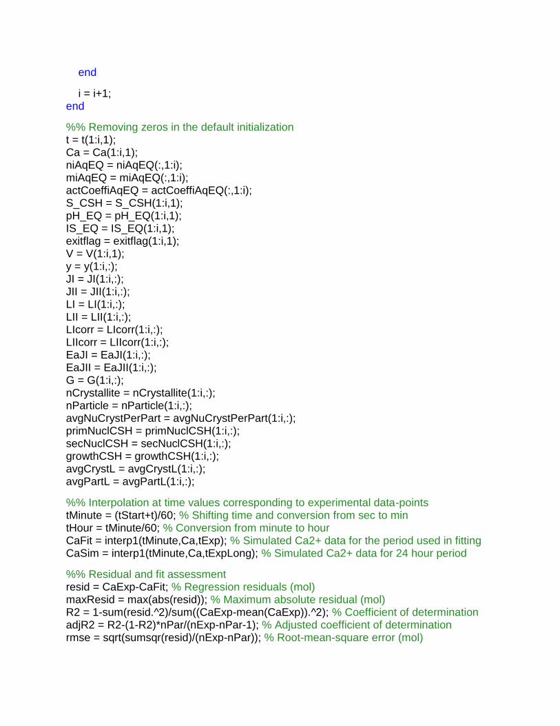
end
i = i+1; end
%% Removing zeros in the default initialization
t = t(1:i,1); Ca = Ca(1:i,1); niAqEQ = niAqEQ(:,1:i); miAqEQ = miAqEQ(:,1:i); actCoeffiAqEQ = actCoeffiAqEQ(:,1:i); S_CSH = S_CSH(1:i,1); pH_EQ = pH_EQ(1:i,1); IS_EQ = IS_EQ(1:i,1); exitflag = exitflag(1:i,1); V = V(1:i,1); y = y(1:i,:); JI = JI(1:i,:); JII = JII(1:i,:); LI = LI(1:i,:); LII = LII(1:i,:); LIcorr = LIcorr(1:i,:); LIIcorr = LIIcorr(1:i,:); EaJI = EaJI(1:i,:); EaJII = EaJII(1:i,:); G = G(1:i,:); nCrystallite = nCrystallite(1:i,:); nParticle = nParticle(1:i,:); avgNuCrystPerPart = avgNuCrystPerPart(1:i,:); primNuclCSH = primNuclCSH(1:i,:); secNuclCSH = secNuclCSH(1:i,:); growthCSH = growthCSH(1:i,:); avgCrystL = avgCrystL(1:i,:); avgPartL = avgPartL(1:i,:); %% Interpolation at time values corresponding to experimental data-points
tMinute = (tStart+t)/60; % Shifting time and conversion from sec to min
tHour = tMinute/60; % Conversion from minute to hour
CaFit = interp1(tMinute,Ca,tExp); % Simulated Ca2+ data for the period used in fitting
CaSim = interp1(tMinute,Ca,tExpLong); % Simulated Ca2+ data for 24 hour period
%% Residual and fit assessment resid = CaExp-CaFit; % Regression residuals (mol)
maxResid = max(abs(resid)); % Maximum absolute residual (mol)
R2 = 1-sum(resid.^2)/sum((CaExp-mean(CaExp)).^2); % Coefficient of determination
adjR2 = R2-(1-R2)*nPar/(nExp-nPar-1); % Adjusted coefficient of determination
rmse = sqrt(sumsqr(resid)/(nExp-nPar)); % Root-mean-square error (mol)
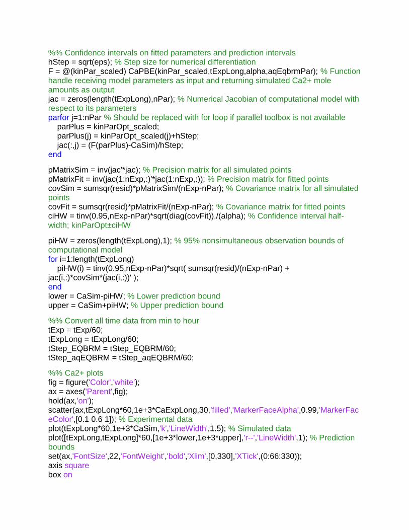
%% Confidence intervals on fitted parameters and prediction intervals
hStep = sqrt(eps); % Step size for numerical differentiation
F = @(kinPar_scaled) CaPBE(kinPar_scaled,tExpLong,alpha,aqEqbrmPar); % Function handle receiving model parameters as input and returning simulated Ca2+ mole amounts as output jac = zeros(length(tExpLong),nPar); % Numerical Jacobian of computational model with respect to its parameters
parfor j=1:nPar % Should be replaced with for loop if parallel toolbox is not available
parPlus = kinParOpt_scaled; parPlus(j) = kinParOpt_scaled(j)+hStep; jac(:,j) = (F(parPlus)-CaSim)/hStep; end
pMatrixSim = inv(jac'*jac); % Precision matrix for all simulated points
pMatrixFit = inv(jac(1:nExp,:)'*jac(1:nExp,:)); % Precision matrix for fitted points
covSim = sumsqr(resid)*pMatrixSim/(nExp-nPar); % Covariance matrix for all simulated points
covFit = sumsqr(resid)*pMatrixFit/(nExp-nPar); % Covariance matrix for fitted points
ciHW = tinv(0.95,nExp-nPar)*sqrt(diag(covFit))./(alpha); % Confidence interval half-width; kinParOpt±ciHW
piHW = zeros(length(tExpLong),1); % 95% nonsimultaneous observation bounds of computational model for i=1:length(tExpLong)
piHW(i) = tinv(0.95,nExp-nPar)*sqrt( sumsqr(resid)/(nExp-nPar) + jac(i,:)*covSim*(jac(i,:))' ); end
lower = CaSim-piHW; % Lower prediction bound
upper = CaSim+piHW; % Upper prediction bound
%% Convert all time data from min to hour
tExp = tExp/60; tExpLong = tExpLong/60; tStep_EQBRM = tStep_EQBRM/60; tStep_aqEQBRM = tStep_aqEQBRM/60; %% Ca2+ plots
fig = figure('Color','white'); ax = axes('Parent',fig); hold(ax,'on'); scatter(ax,tExpLong*60,1e+3*CaExpLong,30,'filled','MarkerFaceAlpha',0.99,'MarkerFaceColor',[0.1 0.6 1]); % Experimental data
plot(tExpLong*60,1e+3*CaSim,'k','LineWidth',1.5); % Simulated data
plot([tExpLong,tExpLong]*60,[1e+3*lower,1e+3*upper],'r--','LineWidth',1); % Prediction bounds
set(ax,'FontSize',22,'FontWeight','bold','Xlim',[0,330],'XTick',(0:66:330)); axis square
box on
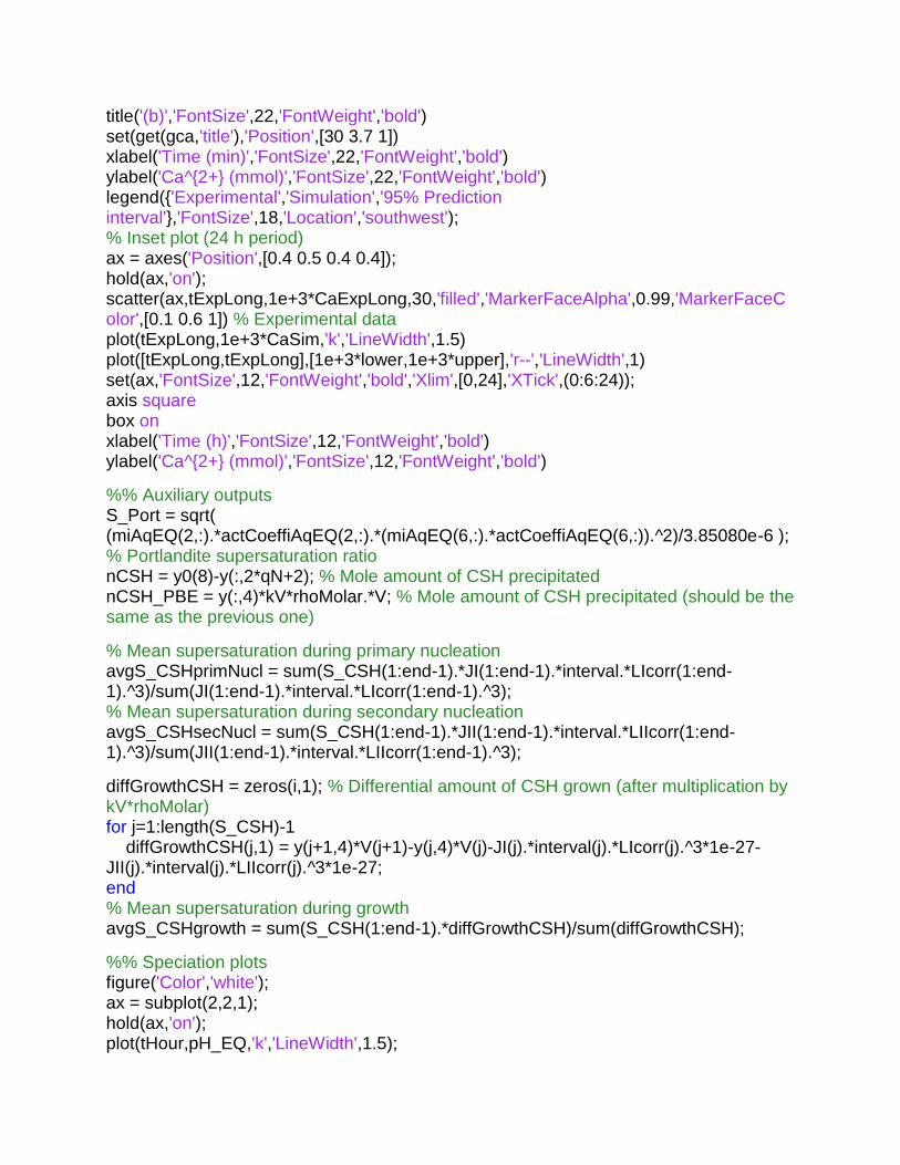
title('(b)','FontSize',22,'FontWeight','bold')
set(get(gca,'title'),'Position',[30 3.7 1])
xlabel('Time (min)','FontSize',22,'FontWeight','bold')
ylabel('Ca^{2+} (mmol)','FontSize',22,'FontWeight','bold')
legend({'Experimental','Simulation','95% Prediction interval'},'FontSize',18,'Location','southwest'); % Inset plot (24 h period)
ax = axes('Position',[0.4 0.5 0.4 0.4]); hold(ax,'on'); scatter(ax,tExpLong,1e+3*CaExpLong,30,'filled','MarkerFaceAlpha',0.99,'MarkerFaceColor',[0.1 0.6 1]) % Experimental data
plot(tExpLong,1e+3*CaSim,'k','LineWidth',1.5)
plot([tExpLong,tExpLong],[1e+3*lower,1e+3*upper],'r--','LineWidth',1)
set(ax,'FontSize',12,'FontWeight','bold','Xlim',[0,24],'XTick',(0:6:24)); axis square
box on
xlabel('Time (h)','FontSize',12,'FontWeight','bold')
ylabel('Ca^{2+} (mmol)','FontSize',12,'FontWeight','bold')
%% Auxiliary outputs
S_Port = sqrt( (miAqEQ(2,:).*actCoeffiAqEQ(2,:).*(miAqEQ(6,:).*actCoeffiAqEQ(6,:)).^2)/3.85080e-6 ); % Portlandite supersaturation ratio
nCSH = y0(8)-y(:,2*qN+2); % Mole amount of CSH precipitated
nCSH_PBE = y(:,4)*kV*rhoMolar.*V; % Mole amount of CSH precipitated (should be the same as the previous one)
% Mean supersaturation during primary nucleation
avgS_CSHprimNucl = sum(S_CSH(1:end-1).*JI(1:end-1).*interval.*LIcorr(1:end-1).^3)/sum(JI(1:end-1).*interval.*LIcorr(1:end-1).^3); % Mean supersaturation during secondary nucleation
avgS_CSHsecNucl = sum(S_CSH(1:end-1).*JII(1:end-1).*interval.*LIIcorr(1:end-1).^3)/sum(JII(1:end-1).*interval.*LIIcorr(1:end-1).^3); diffGrowthCSH = zeros(i,1); % Differential amount of CSH grown (after multiplication by kV*rhoMolar)
for j=1:length(S_CSH)-1
diffGrowthCSH(j,1) = y(j+1,4)*V(j+1)-y(j,4)*V(j)-JI(j).*interval(j).*LIcorr(j).^3*1e-27-JII(j).*interval(j).*LIIcorr(j).^3*1e-27; end
% Mean supersaturation during growth
avgS_CSHgrowth = sum(S_CSH(1:end-1).*diffGrowthCSH)/sum(diffGrowthCSH); %% Speciation plots
figure('Color','white'); ax = subplot(2,2,1); hold(ax,'on'); plot(tHour,pH_EQ,'k','LineWidth',1.5);
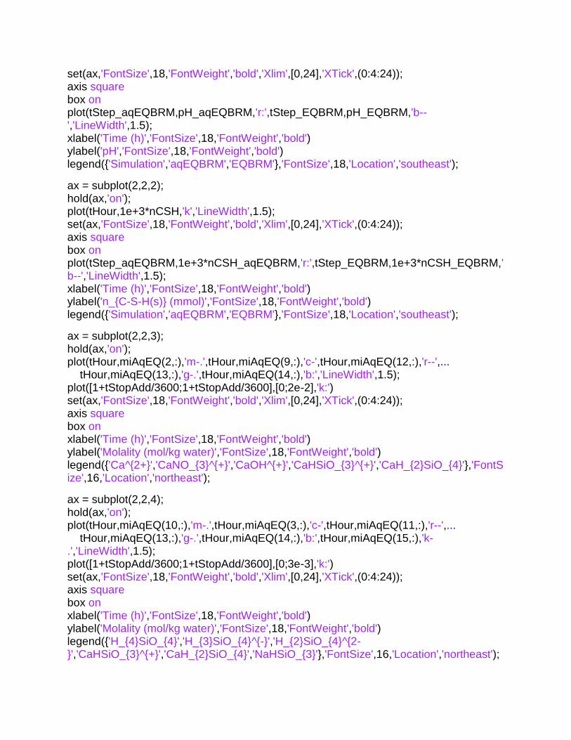
set(ax,'FontSize',18,'FontWeight','bold','Xlim',[0,24],'XTick',(0:4:24)); axis square
box on
plot(tStep_aqEQBRM,pH_aqEQBRM,'r:',tStep_EQBRM,pH_EQBRM,'b--','LineWidth',1.5); xlabel('Time (h)','FontSize',18,'FontWeight','bold')
ylabel('pH','FontSize',18,'FontWeight','bold')
legend({'Simulation','aqEQBRM','EQBRM'},'FontSize',18,'Location','southeast'); ax = subplot(2,2,2); hold(ax,'on'); plot(tHour,1e+3*nCSH,'k','LineWidth',1.5); set(ax,'FontSize',18,'FontWeight','bold','Xlim',[0,24],'XTick',(0:4:24)); axis square
box on
plot(tStep_aqEQBRM,1e+3*nCSH_aqEQBRM,'r:',tStep_EQBRM,1e+3*nCSH_EQBRM,'b--','LineWidth',1.5); xlabel('Time (h)','FontSize',18,'FontWeight','bold')
ylabel('n_{C-S-H(s)} (mmol)','FontSize',18,'FontWeight','bold')
legend({'Simulation','aqEQBRM','EQBRM'},'FontSize',18,'Location','southeast'); ax = subplot(2,2,3); hold(ax,'on'); plot(tHour,miAqEQ(2,:),'m-.',tHour,miAqEQ(9,:),'c-',tHour,miAqEQ(12,:),'r--',... tHour,miAqEQ(13,:),'g-.',tHour,miAqEQ(14,:),'b:','LineWidth',1.5); plot([1+tStopAdd/3600;1+tStopAdd/3600],[0;2e-2],'k:')
set(ax,'FontSize',18,'FontWeight','bold','Xlim',[0,24],'XTick',(0:4:24)); axis square
box on
xlabel('Time (h)','FontSize',18,'FontWeight','bold')
ylabel('Molality (mol/kg water)','FontSize',18,'FontWeight','bold')
legend({'Ca^{2+}','CaNO_{3}^{+}','CaOH^{+}','CaHSiO_{3}^{+}','CaH_{2}SiO_{4}'},'FontSize',16,'Location','northeast'); ax = subplot(2,2,4); hold(ax,'on'); plot(tHour,miAqEQ(10,:),'m-.',tHour,miAqEQ(3,:),'c-',tHour,miAqEQ(11,:),'r--',... tHour,miAqEQ(13,:),'g-.',tHour,miAqEQ(14,:),'b:',tHour,miAqEQ(15,:),'k-.','LineWidth',1.5); plot([1+tStopAdd/3600;1+tStopAdd/3600],[0;3e-3],'k:')
set(ax,'FontSize',18,'FontWeight','bold','Xlim',[0,24],'XTick',(0:4:24)); axis square
box on
xlabel('Time (h)','FontSize',18,'FontWeight','bold')
ylabel('Molality (mol/kg water)','FontSize',18,'FontWeight','bold')
legend({'H_{4}SiO_{4}','H_{3}SiO_{4}^{-}','H_{2}SiO_{4}^{2-}','CaHSiO_{3}^{+}','CaH_{2}SiO_{4}','NaHSiO_{3}'},'FontSize',16,'Location','northeast');
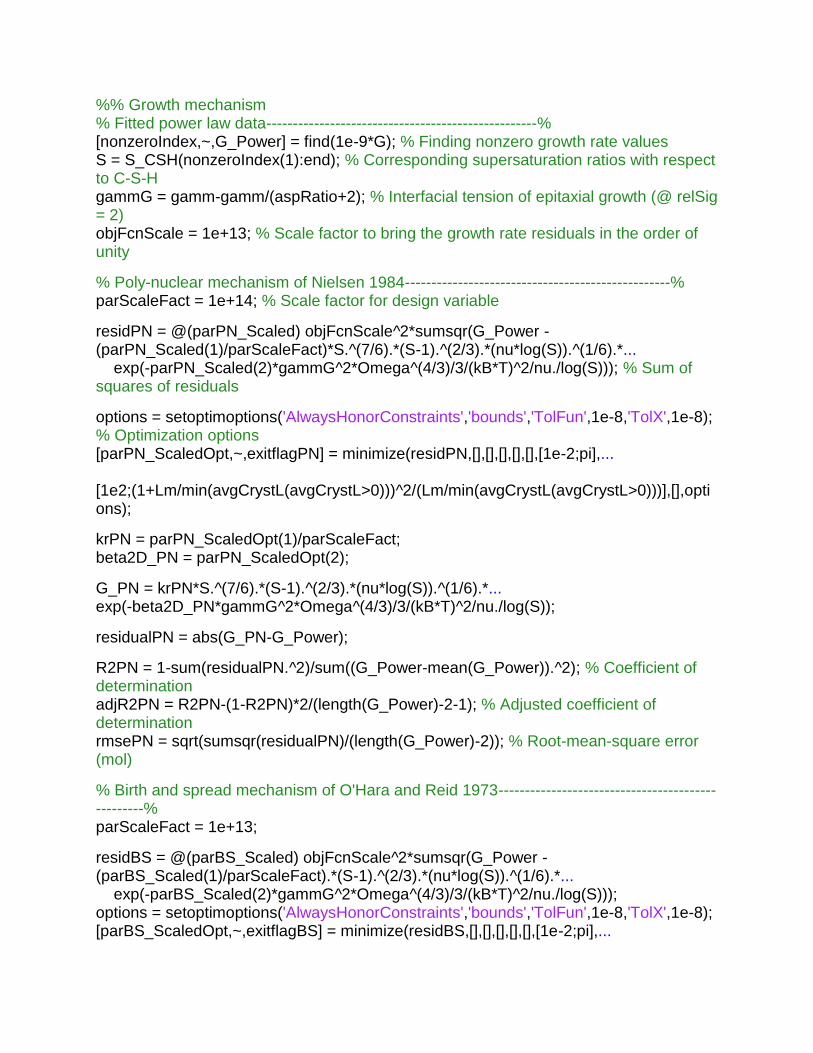
%% Growth mechanism
% Fitted power law data---------------------------------------------------%
[nonzeroIndex,~,G_Power] = find(1e-9*G); % Finding nonzero growth rate values
S = S_CSH(nonzeroIndex(1):end); % Corresponding supersaturation ratios with respect to C-S-H
gammG = gamm-gamm/(aspRatio+2); % Interfacial tension of epitaxial growth (@ relSig = 2)
objFcnScale = 1e+13; % Scale factor to bring the growth rate residuals in the order of unity
% Poly-nuclear mechanism of Nielsen 1984--------------------------------------------------%
parScaleFact = 1e+14; % Scale factor for design variable
residPN = @(parPN_Scaled) objFcnScale^2*sumsqr(G_Power - (parPN_Scaled(1)/parScaleFact)*S.^(7/6).*(S-1).^(2/3).*(nu*log(S)).^(1/6).*... exp(-parPN_Scaled(2)*gammG^2*Omega^(4/3)/3/(kB*T)^2/nu./log(S))); % Sum of squares of residuals
options = setoptimoptions('AlwaysHonorConstraints','bounds','TolFun',1e-8,'TolX',1e-8); % Optimization options
[parPN_ScaledOpt,~,exitflagPN] = minimize(residPN,[],[],[],[],[],[1e-2;pi],... [1e2;(1+Lm/min(avgCrystL(avgCrystL>0)))^2/(Lm/min(avgCrystL(avgCrystL>0)))],[],options); krPN = parPN_ScaledOpt(1)/parScaleFact; beta2D_PN = parPN_ScaledOpt(2); G_PN = krPN*S.^(7/6).*(S-1).^(2/3).*(nu*log(S)).^(1/6).*... exp(-beta2D_PN*gammG^2*Omega^(4/3)/3/(kB*T)^2/nu./log(S));
residualPN = abs(G_PN-G_Power); R2PN = 1-sum(residualPN.^2)/sum((G_Power-mean(G_Power)).^2); % Coefficient of determination
adjR2PN = R2PN-(1-R2PN)*2/(length(G_Power)-2-1); % Adjusted coefficient of determination
rmsePN = sqrt(sumsqr(residualPN)/(length(G_Power)-2)); % Root-mean-square error (mol)
% Birth and spread mechanism of O'Hara and Reid 1973--------------------------------------------------%
parScaleFact = 1e+13; residBS = @(parBS_Scaled) objFcnScale^2*sumsqr(G_Power - (parBS_Scaled(1)/parScaleFact).*(S-1).^(2/3).*(nu*log(S)).^(1/6).*... exp(-parBS_Scaled(2)*gammG^2*Omega^(4/3)/3/(kB*T)^2/nu./log(S))); options = setoptimoptions('AlwaysHonorConstraints','bounds','TolFun',1e-8,'TolX',1e-8); [parBS_ScaledOpt,~,exitflagBS] = minimize(residBS,[],[],[],[],[],[1e-2;pi],...
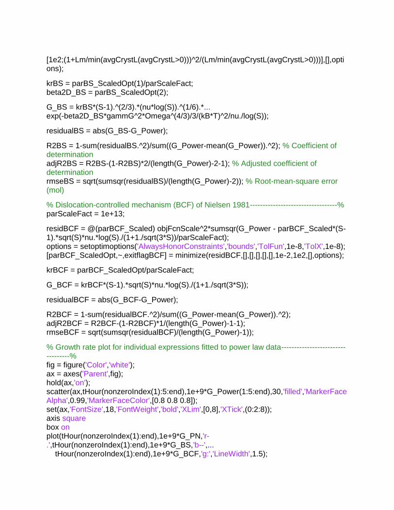
[1e2;(1+Lm/min(avgCrystL(avgCrystL>0)))^2/(Lm/min(avgCrystL(avgCrystL>0)))],[],options); krBS = parBS_ScaledOpt(1)/parScaleFact; beta2D_BS = parBS_ScaledOpt(2); G_BS = krBS*(S-1).^(2/3).*(nu*log(S)).^(1/6).*... exp(-beta2D_BS*gammG^2*Omega^(4/3)/3/(kB*T)^2/nu./log(S));
residualBS = abs(G_BS-G_Power); R2BS = 1-sum(residualBS.^2)/sum((G_Power-mean(G_Power)).^2); % Coefficient of determination
adjR2BS = R2BS-(1-R2BS)*2/(length(G_Power)-2-1); % Adjusted coefficient of determination
rmseBS = sqrt(sumsqr(residualBS)/(length(G_Power)-2)); % Root-mean-square error (mol)
% Dislocation-controlled mechanism (BCF) of Nielsen 1981----------------------------------%
parScaleFact = 1e+13; residBCF = @(parBCF_Scaled) objFcnScale^2*sumsqr(G_Power - parBCF_Scaled*(S-1).*sqrt(S)*nu.*log(S)./(1+1./sqrt(3*S))/parScaleFact); options = setoptimoptions('AlwaysHonorConstraints','bounds','TolFun',1e-8,'TolX',1e-8); [parBCF_ScaledOpt,~,exitflagBCF] = minimize(residBCF,[],[],[],[],[],1e-2,1e2,[],options); krBCF = parBCF_ScaledOpt/parScaleFact; G_BCF = krBCF*(S-1).*sqrt(S)*nu.*log(S)./(1+1./sqrt(3*S)); residualBCF = abs(G_BCF-G_Power); R2BCF = 1-sum(residualBCF.^2)/sum((G_Power-mean(G_Power)).^2); adjR2BCF = R2BCF-(1-R2BCF)*1/(length(G_Power)-1-1); rmseBCF = sqrt(sumsqr(residualBCF)/(length(G_Power)-1)); % Growth rate plot for individual expressions fitted to power law data----------------------------------%
fig = figure('Color','white'); ax = axes('Parent',fig); hold(ax,'on'); scatter(ax,tHour(nonzeroIndex(1):5:end),1e+9*G_Power(1:5:end),30,'filled','MarkerFaceAlpha',0.99,'MarkerFaceColor',[0.8 0.8 0.8]); set(ax,'FontSize',18,'FontWeight','bold','XLim',[0,8],'XTick',(0:2:8)); axis square
box on
plot(tHour(nonzeroIndex(1):end),1e+9*G_PN,'r-.',tHour(nonzeroIndex(1):end),1e+9*G_BS,'b--',... tHour(nonzeroIndex(1):end),1e+9*G_BCF,'g:','LineWidth',1.5);

scatter(ax,tHour(1:5:nonzeroIndex(1)-1),G(1:5:nonzeroIndex(1)-1),30,'filled','MarkerFaceAlpha',0.99,'MarkerFaceColor',[0.8 0.8 0.8])
xlabel('Time (h)','FontSize',18,'FontWeight','bold')
ylabel('Growth rate (nm/s)','FontSize',18,'FontWeight','bold')
legend({'Power law','Poly-nuclear (Nielsen 1984)','B&S (O`Hara and Reid 1973)','BCF (Nielsen 1981)'},'location','northeast','FontSize',18); % Compound B&S and BCF----------------------------------%
parScaleFact = 1e+13; residComp = @(parComp_Scaled) objFcnScale^2*sumsqr(G_Power - ... (parComp_Scaled(1)/parScaleFact)*(S-1).*sqrt(S)*nu.*log(S)./(1+1./sqrt(3*S)) - ... (parComp_Scaled(2)/parScaleFact)*(S-1).^(2/3).*(nu*log(S)).^(1/6).*... exp(-parComp_Scaled(3)*Omega^(4/3)*gammG^2/3/(kB*T)^2/nu./log(S)));
options = setoptimoptions('AlwaysHonorConstraints','bounds','TolFun',1e-12,'TolX',1e-12); [parComp_ScaledOpt,~,exitflagComp] = minimize(residComp,[],[],[],[],[],[1e-2;1e-2;pi],... [1e2;1e2;(1+Lm/min(avgCrystL(avgCrystL>0)))^2/(Lm/min(avgCrystL(avgCrystL>0)))],[],options); % Alternative optimization function (uncomment for use)
% [parCompOpt_scaled,~,exitflagComp] = fmincon(residComp,[1;1;1],[],[],[],[],[1e-2;1e-2],[1e2;1e2]); krBCF_Comp = parComp_ScaledOpt(1)/parScaleFact; krBS_Comp = parComp_ScaledOpt(2)/parScaleFact; beta2D_Comp = parComp_ScaledOpt(3); G_CompFcn = @(parComp_Scaled) (parComp_Scaled(1)/parScaleFact)*(S-1).*sqrt(S)*nu.*log(S)./(1+1./sqrt(3*S)) + ... (parComp_Scaled(2)/parScaleFact)*(S-1).^(2/3).*(nu*log(S)).^(1/6).*... exp(-parComp_Scaled(3)*Omega^(4/3)*gammG^2/3/(kB*T)^2/nu./log(S));
G_Comp = G_CompFcn(parComp_ScaledOpt); residualComp = abs(G_Comp-G_Power); R2Comp = 1-sum(residualComp.^2)/sum((G_Power-mean(G_Power)).^2); adjR2Comp = R2Comp-(1-R2Comp)*3/(length(G_Power)-3-1); rmseComp = sqrt(sumsqr(residualComp)/(length(G_Power)-3)); % Numerical Jacobian of compound growth rate function with respect to its input parameters
J = zeros(length(G_Power),length(parComp_ScaledOpt)); parfor j=1:length(parComp_ScaledOpt)
parComp_ScaledOptPlus = parComp_ScaledOpt; parComp_ScaledOptPlus(j) = parComp_ScaledOpt(j)+hStep; J(:,j) = (G_CompFcn(parComp_ScaledOptPlus)-G_Comp)/hStep; end

% Confidence intevals for compound growth rate parameters
pMatrixComp = inv(J'*J); % Precision matrix
covComp = sumsqr(residualComp)*pMatrixComp/(length(residualComp)-length(parComp_ScaledOpt)); % Covariance matrix
% Confidence interval half-width; parComp_ScaledOpt±ciHW_Comp
ciHW_Comp = tinv(0.95,length(residualComp)-length(parComp_ScaledOpt))*sqrt(diag(covComp))./[parScaleFact;parScaleFact;1]; %% Growth activation barriers and critical size of 2D nuclei hPlanck = 6.626069934e-34; % Planck constant (J.s)
% BCF activation barrier
EaBCF_LB = -log(hPlanck*krBCF_Comp*4*pi*Lm*gammG*exp(Lm^2*gammG/kB/T)/30/sqrt(KspSI)/solventOmega/NA/(kB*T)^2)*kB*T*NA/1000; EaBCF_UB = -log(hPlanck*krBCF_Comp*4*pi*Lm*gammG*exp(Lm^2*gammG/kB/T)/200/sqrt(KspSI)/solventOmega/NA/(kB*T)^2)*kB*T*NA/1000; % B&S activation barrier
EaBS_LB = -log(hPlanck*krBS_Comp/2/Lm/(30*sqrt(KspSI)/rhoMolar)^(4/3)/exp(-gammG*Lm^2/kB/T)/kB/T)*kB*T*NA/1000; EaBS_UB = -log(hPlanck*krBS_Comp/2/Lm/(200*sqrt(KspSI)/rhoMolar)^(4/3)/exp(-gammG*Lm^2/kB/T)/kB/T)*kB*T*NA/1000; G_Comp_BCF = krBCF_Comp*(S-1).*sqrt(S)*nu.*log(S)./(1+1./sqrt(3*S)); % BCF part of growth rate
G_Comp_BS = krBS_Comp*(S-1).^(2/3).*(nu*log(S)).^(1/6).*... exp(-beta2D_Comp*Omega^(4/3)*gammG^2/3/(kB*T)^2/nu./log(S)); % B&S part of growth rate
% Activation free energy for surface nucleation
[row,~,~] = find(G_Comp_BS(G_Comp_BS>1e-16)); EaSurfNucl_LB = min(1e-3*NA*beta2D_Comp*Omega^(4/3)*gammG^2/(kB*T)/nu./log(S)); EaSurfNucl_UB = 1e-3*NA*beta2D_Comp*Omega^(4/3)*gammG^2/(kB*T)/nu./log(S(max(row)));
% Critical size of surface nuclei L2D = 1e9*2*gammG*Lm^3/kB/T/nu./log(S); % Cylindrical surface nuclei (nm)
% Plot of BCF and B&S components of growth rate along with critical size of
% surface nuclei fig = figure('Color','white'); [ax,hLine1,hLine2] = plotyy([tHour(nonzeroIndex(1):end),tHour(nonzeroIndex(1):end),tHour(nonzeroIndex(1):end)],... 1e9*[G_Comp_BS,G_Comp_BCF,G_Comp],tHour(nonzeroIndex(1):end),L2D); set(fig,'CurrentAxes',ax)
xlabel('Time (h)','FontSize',18,'FontWeight','bold')

ylabel(ax(1),'Growth rate (nm/s)','FontSize',18,'FontWeight','bold') % left y-axis
ylabel(ax(2),'Size of critical surface nuclei (nm)','FontSize',18,'FontWeight','bold','Color',[0.6 0.6 0.6]) % right y-axis
set(hLine1(1),'Color','b','LineStyle','--','LineWidth',1.5); set(hLine1(2),'Color','g','LineStyle',':','LineWidth',1.5); set(hLine1(3),'Color','k','LineStyle','-','LineWidth',1.5); set(hLine2,'Color','r','LineStyle','-.','LineWidth',1); set(ax,'FontSize',18,'FontWeight','bold','XLim',[floor(tHour(nonzeroIndex(1))*10)/10,5],'PlotBoxAspectRatio',[1 1 1]); set(ax(1),'YTick',linspace(0,ceil(max(1e13*G_Comp))*1e-4,6),'YLim',[0,ceil(max(1e13*G_Comp))*1e-4],'YColor','k'); set(ax(2),'YTick',linspace(0,floor(1e9*avgCrystL(end)*aspRatio*10)/10,6),'YLim',[0,floor(1e9*avgCrystL(end)*aspRatio*10)/10],'YColor','r'); legend({'B&S','BCF','Compound B&S+BCF'},'FontSize',18,'Location','north'); fig = figure('Color','white'); [ax,hLine1,hLine2] = plotyy([tHour(nonzeroIndex(1):end),tHour(nonzeroIndex(1):end)],... 1e9*[G_Comp_BS,G_Comp_BCF],tHour(nonzeroIndex(1):end),G_Comp_BCF./G_Comp_BS); set(fig,'CurrentAxes',ax)
xlabel('Time (h)','FontSize',18,'FontWeight','bold')
ylabel(ax(1),'Growth rate (nm/s)','FontSize',18,'FontWeight','bold') % left y-axis
ylabel(ax(2),'G_{BCF}/G_{B&S}','FontSize',18,'FontWeight','bold','Color',[0.6 0.6 0.6]) % right y-axis
set(hLine1(1),'Color','b','LineStyle','--','LineWidth',1.5); set(hLine1(2),'Color','g','LineStyle',':','LineWidth',1.5); set(hLine2,'Color','r','LineStyle','-.','LineWidth',1); set(ax,'FontSize',18,'FontWeight','bold','XLim',[floor(tHour(nonzeroIndex(1))*10)/10,5],'PlotBoxAspectRatio',[1 1 1]); set(ax(1),'YTick',linspace(0,ceil(max(1e13*G_Comp_BCF))*1e-4,6),'YLim',[0,ceil(max(1e13*G_Comp_BCF))*1e-4],'YColor','k'); set(ax(2),'YTick',linspace(0,6,6),'YLim',[0,6],'YColor','r'); legend({'B&S','BCF','Compound B&S+BCF'},'FontSize',18,'Location','north'); %% Plots of nucleation rates and barriers, growth rate, supersaturation, sizes, and contributions
fig = figure('Color','white'); subplot(1,2,1)
[ax,hLine1,hLine2] = plotyy([tHour,tHour],[log10(JI),log10(JII)],[tHour,tHour],[LI,LII]); set(fig,'CurrentAxes',ax)
xlabel('Time (h)','FontSize',18,'FontWeight','bold')
ylabel(ax(1),'log_{10}(nucleation rate/s^{-1})','FontSize',18,'FontWeight','bold') % left y-axis
ylabel(ax(2),'Thickness of critical nuclei (nm)','FontSize',18,'FontWeight','bold','Color',[0.6 0.6 0.6]) % right y-axis
set(hLine1(1),'Color','b','LineWidth',1.5);

set(hLine1(2),'Color','b','LineStyle','--','LineWidth',1.5); set(hLine2(1),'Color','r','LineWidth',1.5); set(hLine2(2),'Color','r','LineStyle','--','LineWidth',1.5); set(ax,'FontSize',18,'FontWeight','bold','XLim',[0,2.5],'PlotBoxAspectRatio',[1 1 1]); set(ax(1),'YTick',linspace(0,20,6),'YLim',[0,20],'YColor','b'); set(ax(2),'YTick',linspace(0,4,6),'YLim',[0,4],'YColor','r'); legend({'Primary nucleation','Secondary nucleation'},'FontSize',18,'Location','north'); ax = subplot(1,2,2); hold(ax,'on'); plot(tHour,EaJI,'r',tHour,EaJII,'b--','LineWidth',1.5); set(ax,'FontSize',18,'FontWeight','bold','XLim',[0,2.5],'YLim',[0,300]); axis square
box on
xlabel('Time (h)','FontSize',18,'FontWeight','bold')
ylabel('\DeltaG_{max} (kJ/mol)','FontSize',18,'FontWeight','bold')
legend({'Primary nucleation','Secondary nucleation'},'FontSize',18,'Location','south'); figure('Color','white'); ax = subplot(1,2,1); hold(ax,'on'); scatter(ax,[tHour(1:5:nonzeroIndex(1)-1);tHour(nonzeroIndex(1):5:end)],1e+9*[G(1:5:nonzeroIndex(1)-1);G_Power(1:5:end)],... 30,'filled','MarkerFaceAlpha',0.9,'MarkerFaceColor',[0.8 0.8 0.8]); set(ax,'FontSize',18,'FontWeight','bold','XLim',[0,8],'XTick',(0:2:8)); axis square
box on
plot(tHour(nonzeroIndex(1):end),1e+9*G_BS,'b--',... tHour(nonzeroIndex(1):end),1e+9*G_BCF,'g:',... tHour(nonzeroIndex(1):end),1e+9*G_Comp,'k-','LineWidth',1); xlabel('Time (h)','FontSize',18,'FontWeight','bold')
ylabel('Growth rate (nm/s)','FontSize',18,'FontWeight','bold')
legend({'Power law','B&S','BCF','BCF+B&S'},'location','northeast','FontSize',18); ax = subplot(1,2,2); hold(ax,'on'); plot(tHour,S_CSH,'b',tHour,S_Port,'r--',[0,24],[1,1],'k:','LineWidth',1.5); set(ax,'FontSize',18,'FontWeight','bold','Xlim',[0,24],'XTick',(0:4:24)); axis square
box on
xlabel('Time (h)','FontSize',18,'FontWeight','bold')
ylabel('Supersaturation ratio','FontSize',18,'FontWeight','bold')
legend({'C-S-H','Portlandite'},'FontSize',18); fig = figure('Color','white'); ax = subplot(1,2,1); hold(ax,'on'); [ax,hLine1,hLine2] = plotyy(tHour,1e+9*avgCrystL,tHour,1e+9*avgPartL);
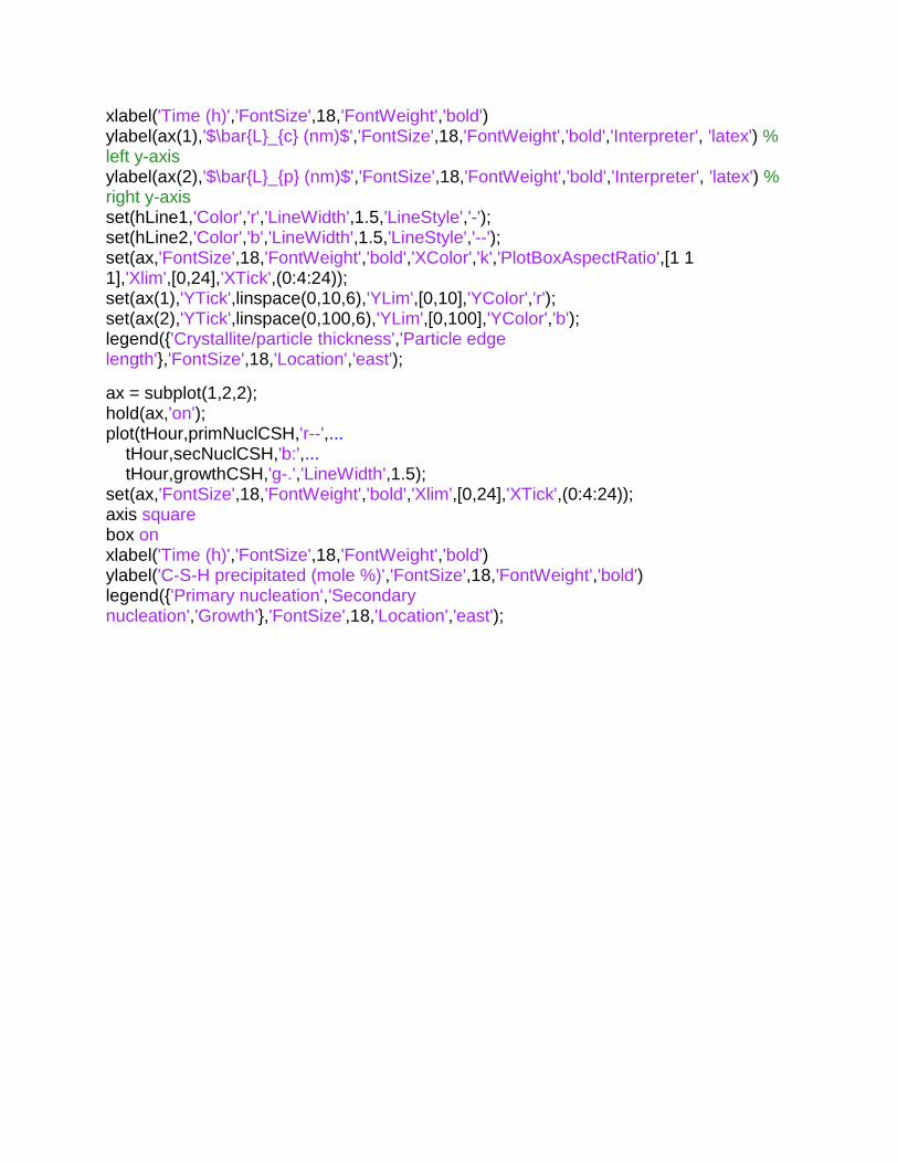
xlabel('Time (h)','FontSize',18,'FontWeight','bold')
ylabel(ax(1),'$\bar{L}_{c} (nm)$','FontSize',18,'FontWeight','bold','Interpreter', 'latex') % left y-axis
ylabel(ax(2),'$\bar{L}_{p} (nm)$','FontSize',18,'FontWeight','bold','Interpreter', 'latex') % right y-axis
set(hLine1,'Color','r','LineWidth',1.5,'LineStyle','-'); set(hLine2,'Color','b','LineWidth',1.5,'LineStyle','--'); set(ax,'FontSize',18,'FontWeight','bold','XColor','k','PlotBoxAspectRatio',[1 1 1],'Xlim',[0,24],'XTick',(0:4:24)); set(ax(1),'YTick',linspace(0,10,6),'YLim',[0,10],'YColor','r'); set(ax(2),'YTick',linspace(0,100,6),'YLim',[0,100],'YColor','b'); legend({'Crystallite/particle thickness','Particle edge length'},'FontSize',18,'Location','east'); ax = subplot(1,2,2); hold(ax,'on'); plot(tHour,primNuclCSH,'r--',... tHour,secNuclCSH,'b:',... tHour,growthCSH,'g-.','LineWidth',1.5); set(ax,'FontSize',18,'FontWeight','bold','Xlim',[0,24],'XTick',(0:4:24)); axis square
box on
xlabel('Time (h)','FontSize',18,'FontWeight','bold')
ylabel('C-S-H precipitated (mole %)','FontSize',18,'FontWeight','bold')
legend({'Primary nucleation','Secondary nucleation','Growth'},'FontSize',18,'Location','east');
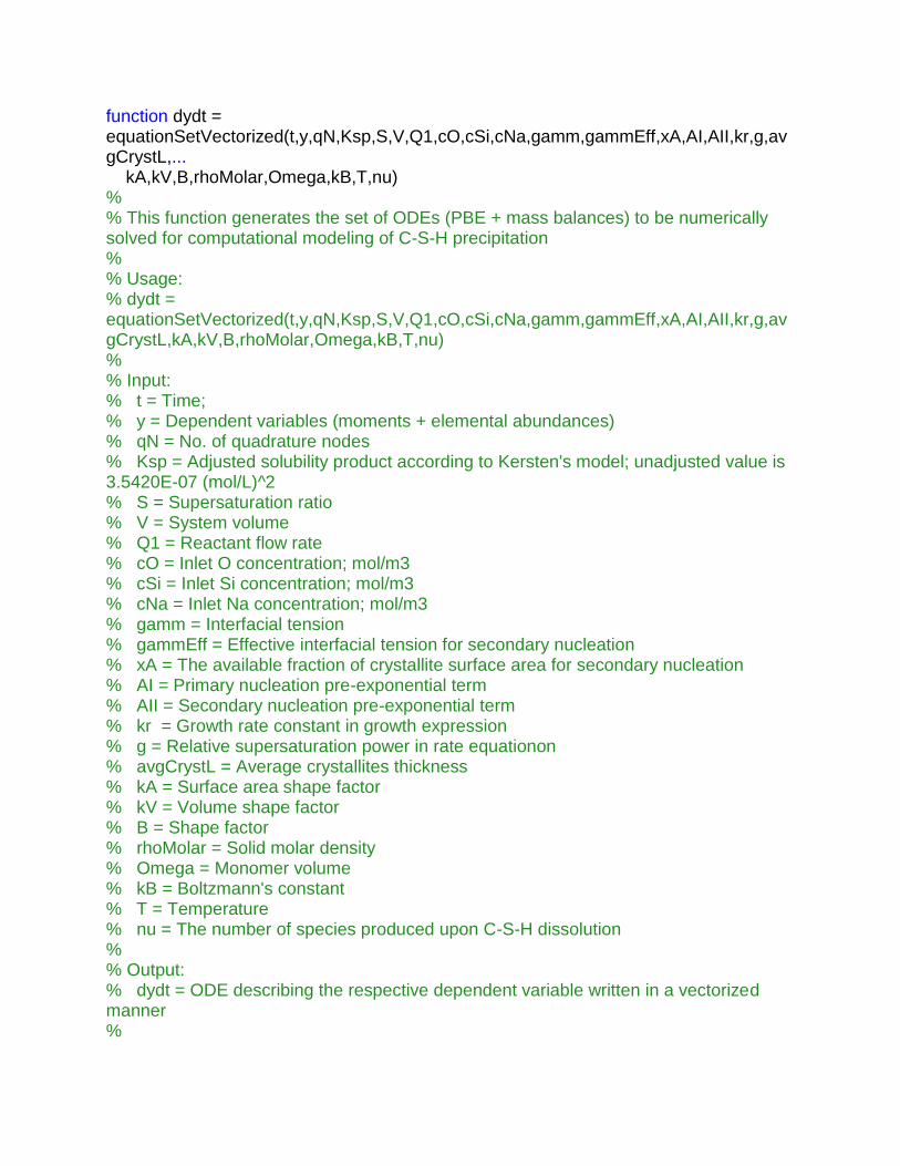
function dydt = equationSetVectorized(t,y,qN,Ksp,S,V,Q1,cO,cSi,cNa,gamm,gammEff,xA,AI,AII,kr,g,avgCrystL,... kA,kV,B,rhoMolar,Omega,kB,T,nu)
% % This function generates the set of ODEs (PBE + mass balances) to be numerically solved for computational modeling of C-S-H precipitation % % Usage: % dydt = equationSetVectorized(t,y,qN,Ksp,S,V,Q1,cO,cSi,cNa,gamm,gammEff,xA,AI,AII,kr,g,avgCrystL,kA,kV,B,rhoMolar,Omega,kB,T,nu) % % Input: % t = Time; % y = Dependent variables (moments + elemental abundances)
% qN = No. of quadrature nodes
% Ksp = Adjusted solubility product according to Kersten's model; unadjusted value is 3.5420E-07 (mol/L)^2
% S = Supersaturation ratio
% V = System volume
% Q1 = Reactant flow rate
% cO = Inlet O concentration; mol/m3
% cSi = Inlet Si concentration; mol/m3
% cNa = Inlet Na concentration; mol/m3
% gamm = Interfacial tension
% gammEff = Effective interfacial tension for secondary nucleation
% xA = The available fraction of crystallite surface area for secondary nucleation
% AI = Primary nucleation pre-exponential term
% AII = Secondary nucleation pre-exponential term
% kr = Growth rate constant in growth expression
% g = Relative supersaturation power in rate equationon
% avgCrystL = Average crystallites thickness
% kA = Surface area shape factor
% kV = Volume shape factor
% B = Shape factor
% rhoMolar = Solid molar density
% Omega = Monomer volume
% kB = Boltzmann's constant % T = Temperature
% nu = The number of species produced upon C-S-H dissolution
% % Output: % dydt = ODE describing the respective dependent variable written in a vectorized manner
%

% This function is part of the MATLAB workflow on "population balance modeling of calcium-silicate-hydrate precipitaion" developed by M. Reza Andalibi at Paul Scherrer Institute/EPFL (2017). % Please cite our article: % M. Reza Andalibi et al., "On The Mesoscale Mechanism of Calcium-Silicate-Hydrate Precipitation: A Population Balance Modeling Approach", 2017. %% Initialization
yNo = size(y,2); % Number of y vectors
dydt = zeros(4+2*qN,yNo); % Initialization
%% Unit correction for Ksp from (mol/L)^nu to SI unit KspSI = Ksp*1000^nu; % Solubility product in SI units (mol/m3)^nu
%% Discretized growth expression in PBE
Li = zeros(qN,yNo); % Quadrature nodes
wi = zeros(qN,yNo); % Quadrature weights
for j=1:yNo
[Li(:,j),wi(:,j)] = WH(y(1:2*qN,j),qN); % NDF construction from moments by Wheeler algorithm
end
if avgCrystL>0 % At least 1 crystallite has formed
Gi = kA*kr*KspSI^(g/nu)*(S-1)^g/(3*kV*rhoMolar); else
Gi = 0; end
%% ODEs for moments
if S<=1 % Zero nucleation rate for (under-)saturated solutions
JI = zeros(1,yNo); JII = zeros(1,yNo); LI = ones(1,yNo); LII = ones(1,yNo); else
LI = ( 2*kA*Omega*gamm/3/kV/kB/T/nu/log(S) )*ones(1,yNo); % m
JI = ( AI*(nu*log(S))^2*exp(-B*gamm^3*Omega^2/kB^3/T^3/nu^2/log(S)^2) )*ones(1,yNo); % #/(m3*s)
% Primary nucleation
A = kA*y(3,:); % Total crystallite surface area
LII = ( 2*kA*Omega*gammEff/3/kV/kB/T/nu/log(S) )*ones(1,yNo); % m
JII = AII*(nu*log(S))^2*xA*A*exp(-B*gammEff^3*Omega^2/kB^3/T^3/nu^2/log(S)^2); % #/(m3*s)
% True secondary nucleation
end
for i=1:2*qN
k = i-1; % Moment order (0,...,2qN-1)
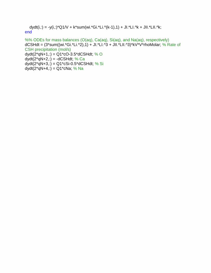
dydt(i,:) = -y(i,:)*Q1/V + k*sum(wi.*Gi.*Li.^(k-1),1) + JI.*LI.^k + JII.*LII.^k; end
%% ODEs for mass balances (O(aq), Ca(aq), Si(aq), and Na(aq), respectively)
dCSHdt = (3*sum((wi.*Gi.*Li.^2),1) + JI.*LI.^3 + JII.*LII.^3)*kV*V*rhoMolar; % Rate of CSH precipitation (mol/s)
dydt(2*qN+1,:) = Q1*cO-3.5*dCSHdt; % O
dydt(2*qN+2,:) = -dCSHdt; % Ca
dydt(2*qN+3,:) = Q1*cSi-0.5*dCSHdt; % Si dydt(2*qN+4,:) = Q1*cNa; % Na
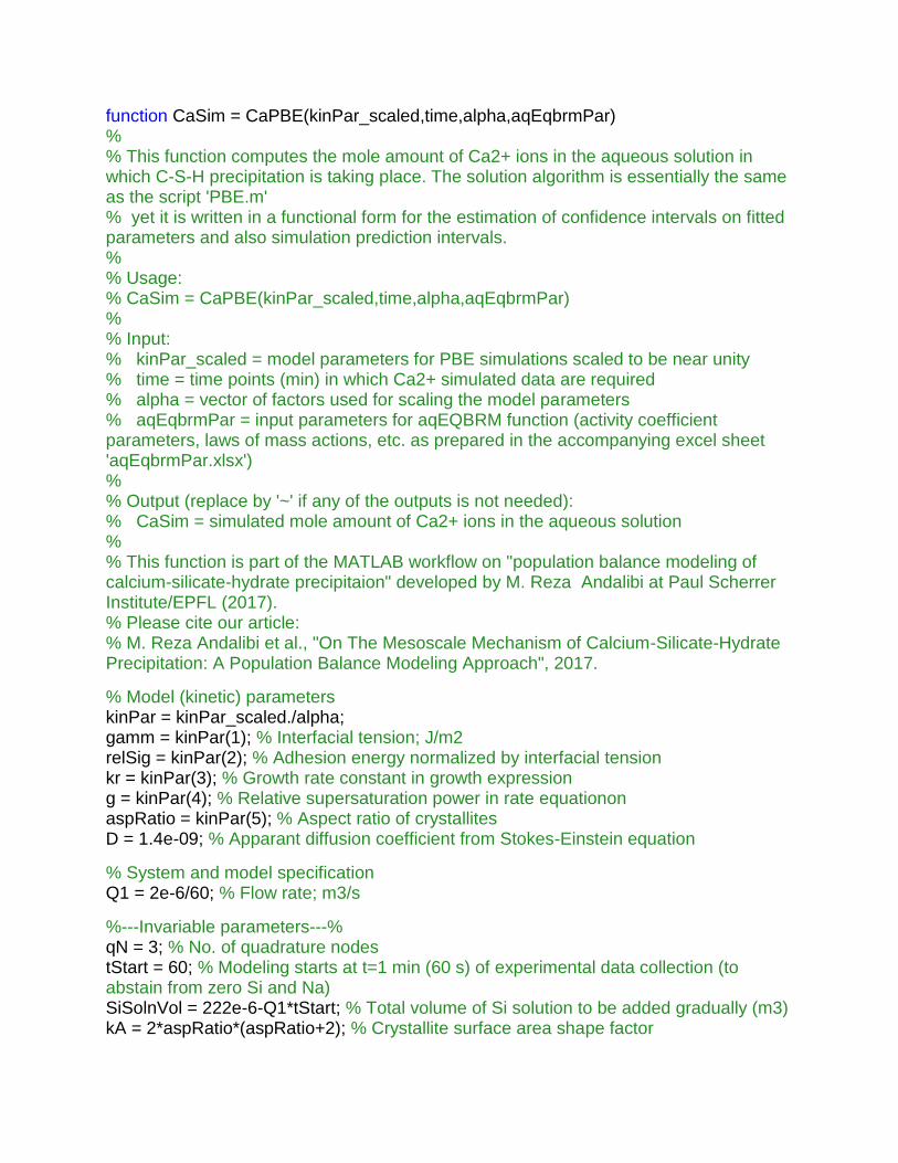
function CaSim = CaPBE(kinPar_scaled,time,alpha,aqEqbrmPar)
% % This function computes the mole amount of Ca2+ ions in the aqueous solution in which C-S-H precipitation is taking place. The solution algorithm is essentially the same as the script 'PBE.m' % yet it is written in a functional form for the estimation of confidence intervals on fitted parameters and also simulation prediction intervals.
% % Usage: % CaSim = CaPBE(kinPar_scaled,time,alpha,aqEqbrmPar)
% % Input: % kinPar_scaled = model parameters for PBE simulations scaled to be near unity
% time = time points (min) in which Ca2+ simulated data are required
% alpha = vector of factors used for scaling the model parameters
% aqEqbrmPar = input parameters for aqEQBRM function (activity coefficient parameters, laws of mass actions, etc. as prepared in the accompanying excel sheet 'aqEqbrmPar.xlsx')
% % Output (replace by '~' if any of the outputs is not needed): % CaSim = simulated mole amount of Ca2+ ions in the aqueous solution
% % This function is part of the MATLAB workflow on "population balance modeling of calcium-silicate-hydrate precipitaion" developed by M. Reza Andalibi at Paul Scherrer Institute/EPFL (2017). % Please cite our article: % M. Reza Andalibi et al., "On The Mesoscale Mechanism of Calcium-Silicate-Hydrate Precipitation: A Population Balance Modeling Approach", 2017. % Model (kinetic) parameters
kinPar = kinPar_scaled./alpha; gamm = kinPar(1); % Interfacial tension; J/m2
relSig = kinPar(2); % Adhesion energy normalized by interfacial tension
kr = kinPar(3); % Growth rate constant in growth expression
g = kinPar(4); % Relative supersaturation power in rate equationon
aspRatio = kinPar(5); % Aspect ratio of crystallites
D = 1.4e-09; % Apparant diffusion coefficient from Stokes-Einstein equation
% System and model specification
Q1 = 2e-6/60; % Flow rate; m3/s
%---Invariable parameters---%
qN = 3; % No. of quadrature nodes
tStart = 60; % Modeling starts at t=1 min (60 s) of experimental data collection (to abstain from zero Si and Na)
SiSolnVol = 222e-6-Q1*tStart; % Total volume of Si solution to be added gradually (m3)
kA = 2*aspRatio*(aspRatio+2); % Crystallite surface area shape factor
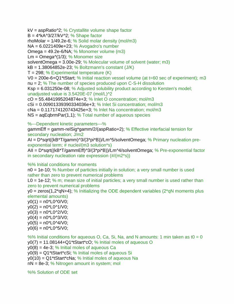
kV = aspRatio^2; % Crystallite volume shape factor
B = 4*kA^3/27/kV^2; % Shape factor
rhoMolar = 1/49.2e-6; % Solid molar density (mol/m3)
NA = 6.0221409e+23; % Avogadro's number
Omega = 49.2e-6/NA; % Monomer volume (m3)
Lm = Omega^(1/3); % Monomer size
solventOmega = 3.00e-29; % Molecular volume of solvent (water; m3)
kB = 1.38064852e-23; % Boltzmann's constant (J/K)
T = 298; % Experimental temperature (K)
V0 = 200e-6+Q1*tStart; % Initial reaction vessel volume (at t=60 sec of experiment); m3
nu = 2; % The number of species produced upon C-S-H dissolution
Ksp = 6.031250e-08; % Adjusted solubility product according to Kersten's model; unadjusted value is 3.5420E-07 (mol/L)^2
cO = 55.4841995204874e+3; % Inlet O concentration; mol/m3
cSi = 0.00901339390334036e+3; % Inlet Si concentration; mol/m3
cNa = 0.117174120743425e+3; % Inlet Na concentration; mol/m3
NS = aqEqbrmPar(1,1); % Total number of aqueous species
%---Dependent kinetic parameters---%
gammEff = gamm-relSig*gamm/2/(aspRatio+2); % Effective interfacial tension for secondary nucleation; J/m2
AI = D*sqrt((kB*T/gamm)^3/(3*pi*B))/Lm^5/solventOmega; % Primary nucleation pre-exponential term; # nuclei/(m3 solution*s)
AII = D*sqrt((kB*T/gammEff)^3/(3*pi*B))/Lm^4/solventOmega; % Pre-exponential factor in secondary nucleation rate expression (#/(m2*s))
%% Initial conditions for moments
n0 = 1e-10; % Number of particles initially in solution; a very small number is used rather than zero to prevent numerical problems
L0 = 1e-12; % m; mean size of initial particles; a very small number is used rather than zero to prevent numerical problems
y0 = zeros(1,2*qN+4); % Initializing the ODE dependent variables (2*qN moments plus elemental amounts)
y0(1) = n0*L0^0/V0; y0(2) = n0*L0^1/V0; y0(3) = n0*L0^2/V0; y0(4) = n0*L0^3/V0; y0(5) = n0*L0^4/V0; y0(6) = n0*L0^5/V0; %% Initial conditions for aqueous O, Ca, Si, Na, and N amounts: 1 min taken as t0 = 0
y0(7) = 11.08144+Q1*tStart*cO; % Initial moles of aqueous O
y0(8) = 4e-3; % Initial moles of aqueous Ca
y0(9) = Q1*tStart*cSi; % Initial moles of aqueous Si y0(10) = Q1*tStart*cNa; % Initial moles of aqueous Na
nN = 8e-3; % Nitrogen amount in system; mol %% Solution of ODE set
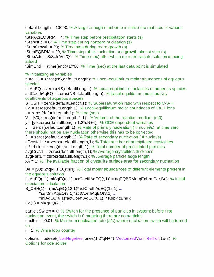
defaultLength = 10000; % A large enough number to initialize the matrices of various variables
tStepAqEQBRM = 4; % Time step before precipitation starts (s)
tStepNucl = 8; % Time step during nonzero nucleation (s)
tStepGrowth = 20; % Time step during mere growth (s)
tStepEQBRM = 20; % Time step after nucleation and growth almost stop (s)
tStopAdd = SiSolnVol/Q1; % Time (sec) after which no more silicate solution is being added
tSimEnd = (time(end)+1)*60; % Time (sec) at the last data point is simulated
% Initializing all variables
niAqEQ = zeros(NS,defaultLength); % Local-equilibrium molar abundaces of aqueous species
miAqEQ = zeros(NS,defaultLength); % Local-equilibrium molalities of aqueous species
actCoeffiAqEQ = zeros(NS,defaultLength); % Local-equilibrium molal activity coefficients of aqueous species
S_CSH = zeros(defaultLength,1); % Supersaturation ratio with respect to C-S-H
Ca = zeros(defaultLength,1); % Local-equilibrium molar abundaces of Ca2+ ions
t = zeros(defaultLength,1); % time (sec)
V = [V0;zeros(defaultLength-1,1)]; % Volume of the reaction medium (m3)
y = [y0;zeros(defaultLength-1,2*qN+4)]; % ODE dependent variables
JI = zeros(defaultLength,1); % Rate of primary nucleation ( # nuclei/s); at time zero there should not be any nucleation otherwise this has to be corrected
JII = zeros(defaultLength,1); % Rate of secondary nucleation ( # nuclei/s)
nCrystallite = zeros(defaultLength,1); % Total number of precipitated crystallites
nParticle = zeros(defaultLength,1); % Total number of precipitated particles
avgCrystL = zeros(defaultLength,1); % Average crystallites thickness
avgPartL = zeros(defaultLength,1); % Average particle edge length
xA = 1; % The available fraction of crystallite surface area for secondary nucleation
Be = [y0(:,2*qN+1:10)';nN]; % Total molar abundances of different elements present in the aqueous solution
[niAqEQ(:,1),miAqEQ(:,1),actCoeffiAqEQ(:,1)] = aqEQBRM(aqEqbrmPar,Be); % Initial speciation calculation
S_CSH(1) = (miAqEQ(12,1)*actCoeffiAqEQ(12,1) ... *sqrt(miAqEQ(3,1)*actCoeffiAqEQ(3,1)... *miAqEQ(6,1)*actCoeffiAqEQ(6,1)) / Ksp)^(1/nu); Ca(1) = niAqEQ(2,1); particleSwitch = 0; % Switch for the presence of particles in system; before first nucleation event, the switch is 0 meaning there are no particles
nuclLim = 0.01; % Minimum nucleation rate (#/s) where nucleation switch will be turned on
i = 1; % While loop counter
options = odeset('NonNegative',ones(1,2*qN+4),'Vectorized','on','RelTol',1e-8); % Options for ode solver
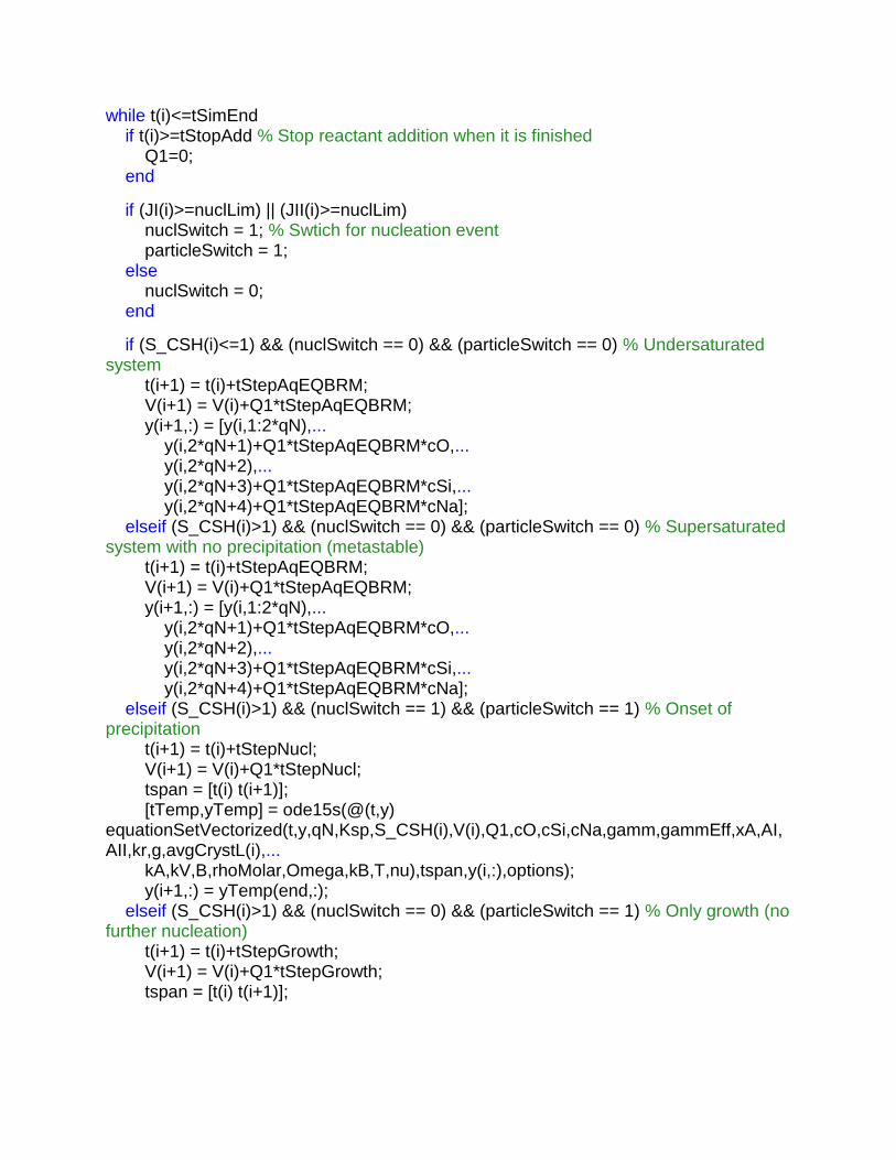
while t(i)<=tSimEnd
if t(i)>=tStopAdd % Stop reactant addition when it is finished
Q1=0; end
if (JI(i)>=nuclLim) || (JII(i)>=nuclLim)
nuclSwitch = 1; % Swtich for nucleation event particleSwitch = 1; else
nuclSwitch = 0; end
if (S_CSH(i)<=1) && (nuclSwitch == 0) && (particleSwitch == 0) % Undersaturated system
t(i+1) = t(i)+tStepAqEQBRM; V(i+1) = V(i)+Q1*tStepAqEQBRM; y(i+1,:) = [y(i,1:2*qN),... y(i,2*qN+1)+Q1*tStepAqEQBRM*cO,... y(i,2*qN+2),... y(i,2*qN+3)+Q1*tStepAqEQBRM*cSi,... y(i,2*qN+4)+Q1*tStepAqEQBRM*cNa]; elseif (S_CSH(i)>1) && (nuclSwitch == 0) && (particleSwitch == 0) % Supersaturated system with no precipitation (metastable)
t(i+1) = t(i)+tStepAqEQBRM; V(i+1) = V(i)+Q1*tStepAqEQBRM; y(i+1,:) = [y(i,1:2*qN),... y(i,2*qN+1)+Q1*tStepAqEQBRM*cO,... y(i,2*qN+2),... y(i,2*qN+3)+Q1*tStepAqEQBRM*cSi,... y(i,2*qN+4)+Q1*tStepAqEQBRM*cNa]; elseif (S_CSH(i)>1) && (nuclSwitch == 1) && (particleSwitch == 1) % Onset of precipitation
t(i+1) = t(i)+tStepNucl; V(i+1) = V(i)+Q1*tStepNucl; tspan = [t(i) t(i+1)]; [tTemp,yTemp] = ode15s(@(t,y) equationSetVectorized(t,y,qN,Ksp,S_CSH(i),V(i),Q1,cO,cSi,cNa,gamm,gammEff,xA,AI,AII,kr,g,avgCrystL(i),... kA,kV,B,rhoMolar,Omega,kB,T,nu),tspan,y(i,:),options); y(i+1,:) = yTemp(end,:); elseif (S_CSH(i)>1) && (nuclSwitch == 0) && (particleSwitch == 1) % Only growth (no further nucleation)
t(i+1) = t(i)+tStepGrowth; V(i+1) = V(i)+Q1*tStepGrowth; tspan = [t(i) t(i+1)];
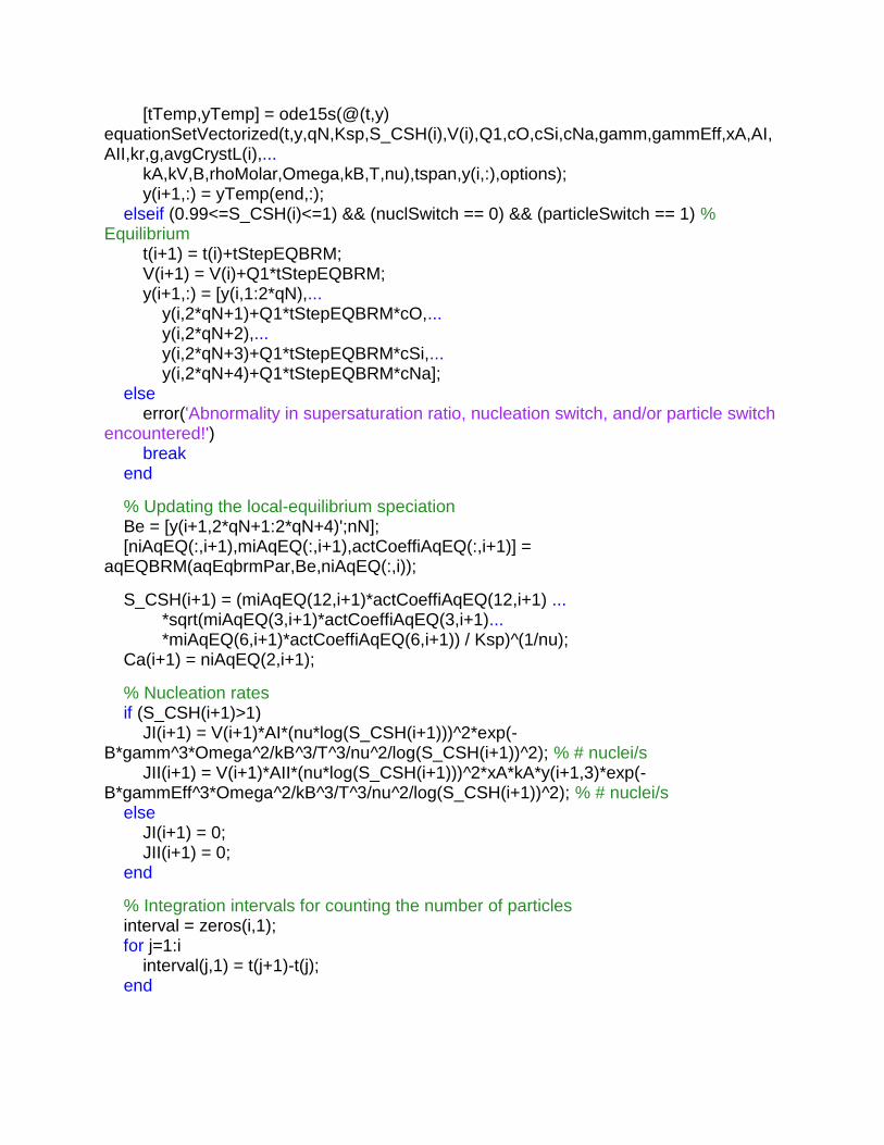
[tTemp,yTemp] = ode15s(@(t,y) equationSetVectorized(t,y,qN,Ksp,S_CSH(i),V(i),Q1,cO,cSi,cNa,gamm,gammEff,xA,AI,AII,kr,g,avgCrystL(i),... kA,kV,B,rhoMolar,Omega,kB,T,nu),tspan,y(i,:),options); y(i+1,:) = yTemp(end,:); elseif (0.99<=S_CSH(i)<=1) && (nuclSwitch == 0) && (particleSwitch == 1) % Equilibrium
t(i+1) = t(i)+tStepEQBRM; V(i+1) = V(i)+Q1*tStepEQBRM; y(i+1,:) = [y(i,1:2*qN),... y(i,2*qN+1)+Q1*tStepEQBRM*cO,... y(i,2*qN+2),... y(i,2*qN+3)+Q1*tStepEQBRM*cSi,... y(i,2*qN+4)+Q1*tStepEQBRM*cNa]; else
error('Abnormality in supersaturation ratio, nucleation switch, and/or particle switch encountered!')
break
end
% Updating the local-equilibrium speciation
Be = [y(i+1,2*qN+1:2*qN+4)';nN]; [niAqEQ(:,i+1),miAqEQ(:,i+1),actCoeffiAqEQ(:,i+1)] = aqEQBRM(aqEqbrmPar,Be,niAqEQ(:,i)); S_CSH(i+1) = (miAqEQ(12,i+1)*actCoeffiAqEQ(12,i+1) ... *sqrt(miAqEQ(3,i+1)*actCoeffiAqEQ(3,i+1)... *miAqEQ(6,i+1)*actCoeffiAqEQ(6,i+1)) / Ksp)^(1/nu); Ca(i+1) = niAqEQ(2,i+1); % Nucleation rates
if (S_CSH(i+1)>1)
JI(i+1) = V(i+1)*AI*(nu*log(S_CSH(i+1)))^2*exp(-B*gamm^3*Omega^2/kB^3/T^3/nu^2/log(S_CSH(i+1))^2); % # nuclei/s
JII(i+1) = V(i+1)*AII*(nu*log(S_CSH(i+1)))^2*xA*kA*y(i+1,3)*exp(-B*gammEff^3*Omega^2/kB^3/T^3/nu^2/log(S_CSH(i+1))^2); % # nuclei/s
else
JI(i+1) = 0; JII(i+1) = 0; end
% Integration intervals for counting the number of particles
interval = zeros(i,1); for j=1:i interval(j,1) = t(j+1)-t(j); end
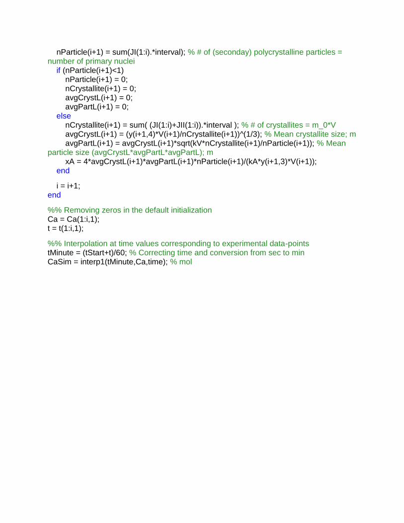
nParticle(i+1) = sum(JI(1:i).*interval); % # of (seconday) polycrystalline particles = number of primary nuclei if (nParticle(i+1)<1)
nParticle(i+1) = 0; nCrystallite(i+1) = 0; avgCrystL(i+1) = 0; avgPartL(i+1) = 0; else
nCrystallite(i+1) = sum( (JI(1:i)+JII(1:i)).*interval ); % # of crystallites = m_0*V
avgCrystL(i+1) = (y(i+1,4)*V(i+1)/nCrystallite(i+1))^(1/3); % Mean crystallite size; m
avgPartL(i+1) = avgCrystL(i+1)*sqrt(kV*nCrystallite(i+1)/nParticle(i+1)); % Mean particle size (avgCrystL*avgPartL*avgPartL); m
xA = 4*avgCrystL(i+1)*avgPartL(i+1)*nParticle(i+1)/(kA*y(i+1,3)*V(i+1));
end
i = i+1; end
%% Removing zeros in the default initialization
Ca = Ca(1:i,1); t = t(1:i,1); %% Interpolation at time values corresponding to experimental data-points
tMinute = (tStart+t)/60; % Correcting time and conversion from sec to min
CaSim = interp1(tMinute,Ca,time); % mol

function [Li,w]=WH(m,N)
% This code was taken from the Appendix A.1.2 of the following reference: % Marchisio, D. L., & Fox, R. O. (2013). Computational models for polydisperse particulate and multiphase systems. Cambridge University Press.
% compute quadrature approximation with the Wheeler algorithm
%
% INPUT: % N = number of nodes of the quadrature approximation
% m = moments from 0 to 2N-1 [mom(1), ..., mom(2N)] %
% OUTPUT: % Li = abscissas
% w = weights
%
% compute intermediate coefficients
%
for l=1:2*N-2
sigma(1,l+1) = 0.0; end
%
for l=0:2*N-1
sigma(2,l+1) = m(l+1); end
%
% compute coefficients for Jacobi matrix
%
a(1) = m(2)/m(1); b(1) = 0.0; %
for k=1:N-1
for l=k:2*N-k-1
sigma(k+2,l+1) = sigma(k+1,l+2)-a(k)*sigma(k+1,l+1)-b(k)*sigma(k,l+1); a(k+1) = -sigma(k+1,k+1)/sigma(k+1,k)+sigma(k+2,k+2)/sigma(k+2,k+1); b(k+1) = sigma(k+2,k+1)/sigma(k+1,k); end
end
% compute Jacobi matrix
%
for i=1:N
jacobi(i,i)=a(i); end
%
for i=1:N-1
jacobi(i,i+1) = -(abs(b(i+1)))^0.5; jacobi(i+1,i) = -(abs(b(i+1)))^0.5; end
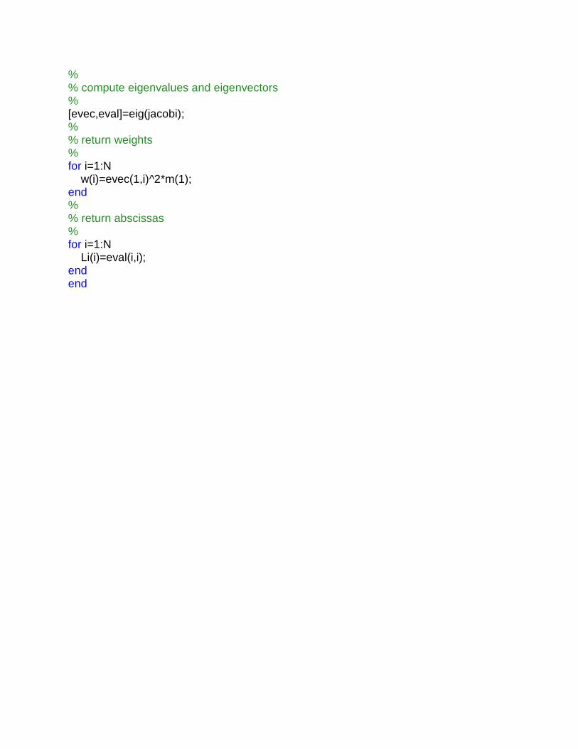
%
% compute eigenvalues and eigenvectors
%
[evec,eval]=eig(jacobi); %
% return weights
%
for i=1:N
w(i)=evec(1,i)^2*m(1); end
%
% return abscissas
%
for i=1:N
Li(i)=eval(i,i); end
end


