the ensemble kalman filter for combined state and ... · shown that the combined parameter and...
TRANSCRIPT

1066-033X/09/$25.00©2009IEEE JUNE 2009 « IEEE CONTROL SYSTEMS MAGAZINE 83
Digital Object Identifier 10.1109/MCS.2009.932223
MONTE CARLO TECHNIQUES FOR DATA ASSIMILATION IN LARGE SYSTEMS
GEIR EVENSEN
The ensemble Kalman fi lter (EnKF) [1] is a sequential Monte Carlo method that provides an alternative to the traditional Kalman fi lter (KF) [2], [3]and adjoint or four-dimensional variational (4DVAR) methods [4]–[6] to better handle large state spaces and nonlinear error evolution. EnKF pro-vides a simple conceptual formulation and ease of implementation, since
there is no need to derive a tangent linear operator or adjoint equations, and there are no integrations backward in time. EnKF is used extensively in a large com-munity, including ocean and atmospheric sciences, oil reservoir simulations, and hydrological modeling.
To a large extent EnKF overcomes two problems associated with the traditional KF. First, in KF an error covariance matrix for the model state needs to be stored and propagated in time, making the method computationally infeasible for mod-els with high-dimensional state vectors. Second, when the model dynamics are nonlinear, the extended KF (EKF) uses a linearized equation for the error covari-ance evolution, and this linearization can result in unbounded linear instabilities for the error evolution [7].
MONTE CARLO TECHNIQUES FOR DATA ASSIMILATION IN LARGE SYSTEMS
The Ensemble Kalman Filter for Combined State and Parameter Estimation
PHOTO COMPOSITE COURTESY OF DAVID STENSRUD
84 IEEE CONTROL SYSTEMS MAGAZINE » JUNE 2009
In contrast with EKF, EnKF represents the error covari-ance matrix by a large stochastic ensemble of model re-alizations. For large systems, the dimensionality problem is managed by using a low-rank approximation of the er-ror covariance matrix, where the number of independent model realizations is less than the number of unknowns in the model. Thus, the uncertainty is represented by a set of model realizations rather than an explicit expression for the error covariance matrix. The ensemble of model states is integrated forward in time to predict error statistics. For linear models the ensemble integration is consistent with the exact integration of an error covariance equation in the limit of an infinite ensemble size. Furthermore, for non-linear dynamical models, the use of an ensemble integra-tion leads to full nonlinear evolution of the error statistics, which in EnKF can be computed with a much lower com-putational cost than in EKF [8].
Whenever measurements are available, each individual realization is updated to incorporate the new information provided by the measurements. Implementations of the up-date schemes can be formulated as either a stochastic [9] or a deterministic scheme [8], [10]–[13]. Both kinds of schemes solve for a variance-minimizing solution and implicitly as-sume that the forecast error statistics are Gaussian by using only the ensemble covariance in the update equation.
The assumption of Gaussian distributions in EnKF al-lows for a linear and efficient update equation to be used. A more sophisticated update scheme needs to be derived to take into account higher order statistics, which leads to particle filtering theory [14], where the Bayes formula is solved at each update step, although normally at a huge computational cost. While the particle filter accounts for non-Gaussian distributions by representing the full pdf in the parameter space, its applicability is normally limited to estimation of a few unknowns at the cost of integrating a very large ensemble consisting of typically more than O (104) realizations.
In [8], EnKF is rederived as a sequential Monte Carlo method starting from a Bayesian formulation. The EnKF can then be characterized as a special case of the particle filter, where the Bayesian update step in the particle fil-ter is approximated with a linear update step in the EnKF using only the two first moments of the predicted prob-ability density function (pdf). With linear dynamics, EnKF is equivalent to a particle filter, since this case is fully de-scribed by Gaussian pdfs. However, with nonlinear dy-namics, non-Gaussian contributions may develop, and the EnKF only approximates the particle filter. Unlike the particle filters [14], EnKF does not need to re-sample the ensemble from the posterior pdf during the analysis step, since each prior model realization is individually updated to create the correct posterior ensemble.
In EnKF, the solution is solved for in the affine space spanned by the ensemble of realizations. The ensemble, which evolves in time according to the nonlinear dynamical
model, provides a representation of the subspace where the update is computed at each analysis time. It is possible to formulate analysis schemes in terms of the ensemble, lead-ing to efficient algorithms where the state error covariance matrix is not computed and is only implicitly used.
A major approximation introduced in EnKF is related to the use of a limited number of ensemble realizations. The ensemble size limits the space where the solution is searched for and in addition introduces spurious correlations that lead to excessive decrease of the ensemble variance and possibly filter divergence. The spurious correlations can be handled by localization methods that attempt to reduce the impact of measurements that are located far from the grid-point to be updated. Localization methods either filter away distant measurements or attempt to reduce the amplitude of the long-range spurious correlations. The use of a local analysis scheme effectively increases the ensemble solution space while reducing the impact of spurious correlations. The use of a local analysis scheme allows for a relatively small ensemble size to be used with a high- dimensional dynamical model.
A chronological list of applications of EnKF is given in [8]. This list includes both low-dimensional systems of highly nonlinear dynamical models as well as high-dimensional ocean and atmospheric circulation models with O (106) or more unknowns. Applications include state estimation in operational circulation models for the ocean and atmosphere as well as parameter estimation or history matching in reservoir simulation models. For ex-ample, [15]–[17] present an implementation of an EnKF with an isopycnal ocean general circulation model, while [18] examines an implementation of a local EnKF with a state-of-the-art operational numerical weather prediction model using simulated measurements. It is shown that a modest-sized ensemble of 40 members can track the evolu-tion of the atmospheric state with high accuracy.
An implementation of the EnKF at the Canadian Meteo-rological Centre in [19] demonstrates EnKF for operational atmospheric data assimilation and reviews EnKF with fo-cus on localization and sampling errors. A review in [20] of a variant of EnKF called the local ensemble transform Kal-man filter includes a derivation of the analysis equations and the numerical implementation, which differ somewhat from what is normally used in the Kalman filtering litera-ture. An implementation of the local ensemble transform Kalman filter with the National Centers for Environmental Prediction (NCEP) global model, given in [21], concludes that the accuracy of the method is competitive with opera-tional algorithms and that this technique can efficiently handle large number of measurements.
An implementation of EnKF with the NCEP model in [22] is compared with the operational NCEP global data as-similation system. The ensemble data assimilation system outperforms a reduced-resolution version of the operation-al three-dimensional variational (3DVAR) data assimilation

JUNE 2009 « IEEE CONTROL SYSTEMS MAGAZINE 85
system and shows improvement in data sparse regions. An observation-thinning algorithm is presented in [22], where observations with little information content leading to low variance reduction are filtered out. The thinning algorithm improves the analysis when unmodeled error correlations are present between nearby observations. The need for the thinning is eliminated if the error correlations are properly specified in the measurement error covariance matrix.
EnKF is currently used in several research fields in addition to the ocean and atmosphere applications cited throughout this article. In [23], the EnKF is used to update a model of tropospheric ozone concentrations and to com-pute short-term air quality forecasts. It is found that the EnKF updated estimates provide improved initial condi-tions and lead to better forecasts of the next day’s ozone concentration maxima. In [24], EnKF is applied to a mag-netohydrodynamic model for space weather prediction. The performance of EnKF in a land surface data assimi-lation experiment is examined in [25]. These results are compared with a sequential importance re-sampling (SIR) filter, and it is found that EnKF performs almost as well as the SIR filter. Furthermore, it is emphasized that EnKF leads to skewed and even multimodal distributions despite the normality assumption imposed when computing the analysis updates.
In this article, we outline the theory behind the EnKF and demonstrate its use in various high-dimensional and nonlinear applications in mathematical physics while also considering the combined parameter and state es-timation problem in some detail. The goal of this article is to serve as an introduction and tutorial for new users of EnKF. We thus present examples that illustrate par-ticular properties of the EnKF, such as its capability to handle high- dimensional state spaces as well as highly nonlinear dynamics.
DATA ASSIMILATION AND PARAMETER ESTIMATIONGiven a dynamical model with initial and boundary con-ditions and a set of measurements that can be related to the model state, the state estimation problem is defined as finding the estimate of the model state that in some weight-ed measure best fits the model equations, the initial and boundary conditions, and the observed data. Unless we relax the equations and allow some or all of the dynami-cal model, the conditions, and the measurements to contain errors, the problem may become overdetermined and no general solution exists.
We often use a prior assumption of Gaussian distribu-tions for the error terms. It is also common to assume that errors in the measurements are uncorrelated with errors in the dynamical model. The problem can then be formulated by using a quadratic cost function whose minimum defines the best estimate of the state.
The parameter estimation problem is different from the state estimation problem. Traditionally, in parameter
estimation we want to improve estimates of a set of poorly known model parameters leading to an exact model solu-tion that is close to the measurements. Thus, in this case we assume that all errors in the model equations are associ-ated with uncertainties in the selected model parameters. The model initial conditions, boundary conditions, and the model structure are all exactly known. Thus, for any set of model parameters the corresponding solution is found from a single forward integration of the model. The way forward is then to define a cost function that measures the distance between the model prediction and the observa-tions plus a term measuring the deviation of the parameter values from a prior estimate of the parameter values. The relative weight between these two terms is determined by the prior error statistics for the measurements and the pri-or parameter estimate. Unfortunately, these problems are often hard to solve [8] since the inverse problem is highly nonlinear, and multiple local minima may be present in the cost function.
In [8] the combined parameter and state estimation problem is considered. An improved state estimate and a set of improved model parameters are then searched for simultaneously. In [26] and [27] this problem is formulated using a variational cost function that is mini-mized using the representer method [28], [29]. Both [26] and [27] report convergence problems due to the non-linearity of the problem and the possible presence of multiple local minima in the cost function. In [8] it is shown that the combined parameter and state estimation problem can be formulated, and in many cases solved efficiently, using ensemble methods. An illustrative ap-plication of the EnKF for combined state and parameter estimation includes estimation of the permeability fields together with dynamic state variables in reservoir simu-lation models [30]. These problems have huge parameter and state spaces with O (106) unknowns. The formula-tion and solution of the combined parameter and state estimation problem using ensemble methods are further discussed below.
REVIEW OF THE KALMAN FILTER
Variance Minimizing Analysis SchemeThe KF is a variance-minimizing algorithm that updates the state estimate whenever measurements are available. The update equations in the KF are normally derived by minimizing the trace of the posterior error covariance ma-trix. The algorithm refers only to first- and second-order statistical moments. With the assumption of Gaussian priors for the model prediction and the data, the update equation can also be derived as the minimizing solution of a quadratic cost function. We start with a vector of vari-ables stored in c (x, t ), which is defined on some spatial domain 'D with spatial coordinate x . When c (x, t ) is discretized on a numerical grid representing the spatial
86 IEEE CONTROL SYSTEMS MAGAZINE » JUNE 2009
model domain, it can be represented by the state vector ck at each time instant tk . The cost function can then be written as
J 3c ka 45 (c k
f 2 c ka )T(Ccc
f ) k21 (c k
f 2 c ka )
1 (dk 2 Mkc ka )T(CPP) k
21 (dk 2 Mk c k
a ), (1)
where c ka and c k
f are the analyzed and forecast estimates respectively, dk is the vector of measurements, Mk is the measurement operator that maps the model state ck to the measurements dk , (Ccc
f ) k is the error covariance of the pre-dicted model state, and (CPP) k is the measurement error co-variance matrix. Minimizing with respect to c k
a yields the classical KF update equations
c ka 5 c k
f 1 Kk(dk 2 Mk c k
f ), (2)
(Ccc) ka 5 (I 2 KkMk) (Ccc) k
f, (3)
Kk 5 (Ccc) kf Mk
T(Mk(Ccc) kf Mk
T 1 (CPP) k) 21, (4)
where the matrix Kk is the Kalman gain. Thus, both the model state and its error covariance are updated.
Kalman FilterIt is assumed that the true state c t evolves in time accord-ing to the dynamical model
c kt 5 Fc k21
t 1 qk21, (5)
where F is a linear model operator and qk21 is the unknown model error over one time step from k 2 1 to k . In this case a numerical model evolves according to
c kf 5 Fc k21
a , (6)
where the superscripts a and f denote analysis and fore-cast. That is, given the best possible estimate (traditionally named analysis) for c at time tk21, a forecast is calculated at time tk , using the approximate equation (6).
The error covariance equation is derived by subtracting (6) from (5), squaring the result, and taking the expecta-tion, which yields
Cccf ( tk) 5 FCa
cc( tk21 )FT 1 Cqq( tk21 ) , (7)
where we define the error covariance matrices for the pre-dicted and analyzed estimates as
Cccf 5 (c f 2 c t ) (c f 2 c t ) T, (8)
Cacc 5 (ca 2 c t ) (ca 2 c t ) T. (9)
The overline denotes an expectation operator, which is equivalent to averaging over an ensemble of infinite size.
Extended Kalman FilterWe now assume a nonlinear model, where the true state vector c k
t at time tk is calculated from
c kt 5 G (c k21
t ) 1 qk21, (10)
and a forecast is calculated from the approximate equation
c kf 5 G (c k21
a ) . (11)
The error statistics then evolve according to the equation
Cfcc( tk) 5 Gk21
r Cacc( tk21 )Gk21
rT 1 Cqq( tk21 ) 1 c, (12)
where Cqq( tk21 ) is the model error covariance matrix and Gk21r is the Jacobian or tangent linear operator given by
Gk21r 5
'G (c )
'c2ck21
. (13)
Note that in (12) we neglect an infinite number of terms containing higher order statistical moments and higher order derivatives of the model operator. EKF is based on the assumption that the contributions from all of the higher order terms are negligible. By discarding these terms we are left with the approximate error covari-ance expression
Cccf ( tk) . Gk21
r Ccca ( tk21 )Gk21
rT 1 Cqq( tk21 ) . (14)
Higher order approximations for the error covariance evo-lution are discussed in [31].
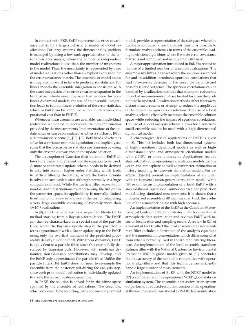
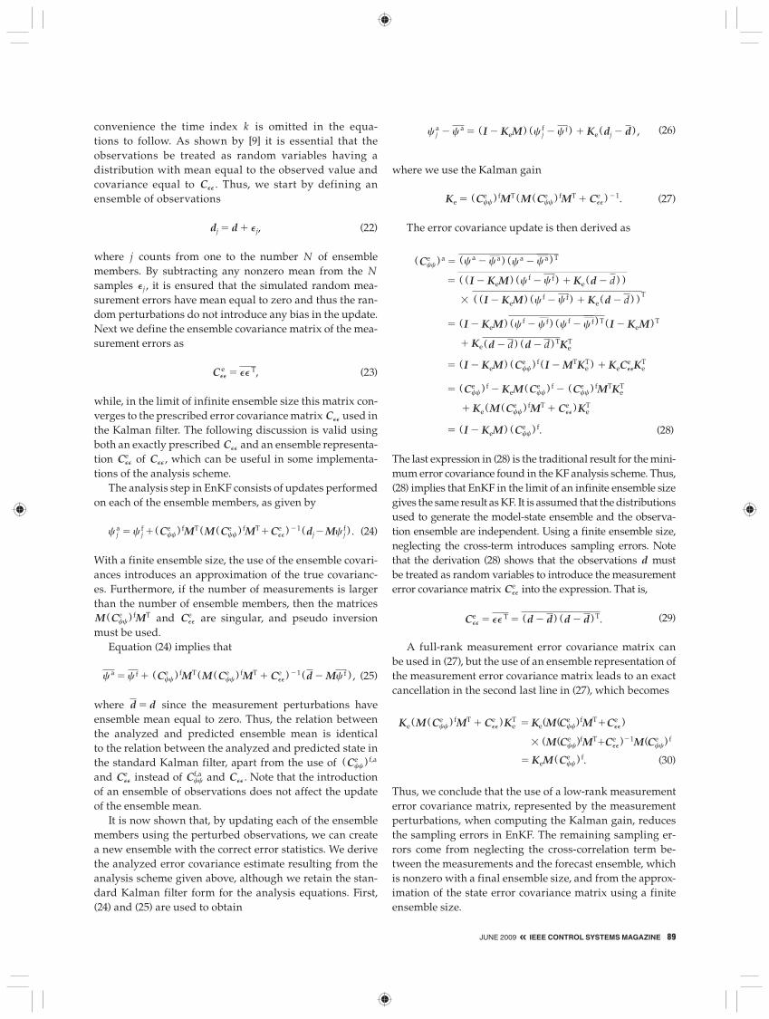
EKF with a Nonlinear Ocean Circulation ModelAs an application of EKF we consider a nonlinear ocean circulation model [7]. The model in Figure 1 is a multilayer quasi-geostrophic model of the mesoscale ocean currents. The quasi-geostrophic model solves simplified fluid equa-tions for the slow motions in the ocean and are formulated in terms of potential vorticity advection in a background velocity field represented by a stream function. Given a change in the vorticity field, at each time step we can solve for the corresponding stream function.
It is found that the linear evolution equation for the er-ror covariance matrix leads to a linear instability. This in-stability is demonstrated in an experiment using a steady background flow defined by an eddy standing on a flat ba-thymetry [see Figure 1(a)]. This particular stream function results in a velocity shear and thus supports a sheared flow instability. Thus, if we add a perturbation and advect it us-ing the linearized equations, then the perturbation grows exponentially. This growth is exactly what is observed in Figure 1(b) and (c). By choosing an initial variance equal to one throughout the model domain, we observe strong
JUNE 2009 « IEEE CONTROL SYSTEMS MAGAZINE 87
error-variance growth at locations of large velocity and velocity shear in the eddy. The estimated mean square errors, which equal the trace of Ccc divided by the number of gridpoints, indicate expo-nential error-variance growth.
This linear instability is not realistic. In the real world we expect the instabil-ity to saturate at a certain climatologi-cal amplitude. As an example, in the atmosphere it is always possible to de-fine a maximum and minimum pres-sure, which is never exceeded, and the same applies for the eddy field in the ocean. An unstable variance growth cannot be accepted but is in fact what the EKF provides in some cases.
Thus, an apparent closure prob-lem is present in the error-covari-ance evolution equation, caused by discarding third- and higher order moments in the error covariance equation, leading to a linear insta-bility. If a correct equation could be used to predict the time evolution of the errors, then linear instabilities would saturate due to nonlinear ef-fects. This saturation is missing in EKF, as confirmed by [32]–[34].
Extended Kalman Filter for the MeanEquations (11), (13), and (14) are the most commonly used for EKF. A weakness of the formulation is that the central forecast is used as the estimate. The central fore-cast is the single model realization initialized with the expected value of the initial state and then integrated by the dynamical model and updated at the measure-ment steps. For nonlinear dynamics the central forecast may not be equal to the expected value, and thus it is just one realization from an infinite ensemble of pos-sible realizations.
An alternative approach is to derive a model for the evo-lution of the first moment or mean. First G (c ) is expanded around c to obtain
G (c ) 5G (c ) 1Gr (c ) (c 2 c ) 112
Grr (c ) (c 2 c ) 2 1 c. (15)
Inserting (15) in (11) and taking the expectation or ensem-ble average yields
ck 5 G (ck21 ) 112
Gk21rr Ccc( tk21 ) 1 c. (16)
It can be argued that for a statistical estimator it makes more sense to work with the mean than a central forecast. After all, the central forecast does not have any statistical interpretation as illustrated by running an atmospheric model without assimilation updates. The central forecast then becomes just one realization out of infinitely many possible realizations, and it is not clear how we can relate the central forecast to the climatological error covariance estimate. On the other hand the equation for the mean provides an estimate that converges to the climatological mean, and the covariance estimate thus describes the er-ror variance of the climatological mean. All applications of the EKF for data assimilation in ocean and atmospheric models use an equation for the central forecast. However, the interpretation using the equation for the mean sup-ports the formulation used in EnKF.
ENSEMBLE KALMAN FILTERWe begin by representing the error statistics using an en-semble of model states. Next, we present an alternative to the traditional error covariance equation for predicting error statistics. Finally, we derive the traditional EnKF analysis scheme.
X-axisY
-axi
s
0 2 4 6 8X-axis
(a) (b)
0 2 4 6 80
2
4
6
8
Y-a
xis
0
2
4
6
8
1.71.51.31.10.90.70.50.30.1
876543210
Time(c)
0 10 20 30 40 501
2
3
Est
imat
ed M
ean
Squ
are
Err
ors
(Non
dim
ensi
onal
)4
5
6
7
FIGURE 1 Example of an extended Kalman filter experiment from [7]. (a) shows the stream function defining the velocity field of a stationary eddy, while (b) shows the resulting error variance in the model domain after integration from t 5 0 to t 5 25. Note the large errors at locations where velocities are high. (c) shows the exponential time evolution of the estimated variance averaged over the model domain.
88 IEEE CONTROL SYSTEMS MAGAZINE » JUNE 2009
Representation of Error StatisticsThe error covariance matrices Ccc
f and Ccca for the
predicted and analyzed estimate in the Kalman filter are defined in terms of the true state in (8) and (9). How-ever, since the true state is not known, we define the en-semble covariance matrices around the ensemble mean c according to
(Ccce ) f5 (c f2c f ) (c f2c f ) T, (17)
(Ccce ) a5 (ca2ca ) (ca2ca )T, (18)
where now the overline denotes an average over the ensem-ble. Thus, we can use an interpretation where the ensemble mean is the best estimate and the spreading of the ensem-ble around the mean is a natural definition of the error in the ensemble mean.
Thus, instead of storing a full covariance matrix, we can represent the same error statistics using an appropriate en-semble of model states. Given an error covariance matrix, an ensemble of finite size provides an approximation to the error covariance matrix, and, as the size N of the ensemble increases, the errors in the Monte Carlo sampling decrease proportionally to 1/"N .
Suppose now that we have N model states or realizations in the ensemble, each of dimension n. Each realization can be represented as a single point in an n-dimensional state space, while together the realizations constitute a cloud of such points. In the limit as N goes to infinity, the cloud of points can be described using the pdf
f(c ) 5dNN
, (19)
where dN is the number of points in a small unit volume and N is the total number of points. Statistical moments can then be calculated from either f(c ) or the ensemble representing f(c ) .
Prediction of Error StatisticsA nonlinear model that contains stochastic errors can be written as the stochastic differential equation
dc5G (c )dt1 h(c )dq. (20)
Equation (20) states that an increment in time yields an in-crement in c , which, in addition, is influenced by a random contribution from the stochastic forcing term h(c )dq , rep-resenting the model errors. The term dq describes a vector Brownian motion process with covariance Cqqdt . Since the model operator G in (20) is not an explicit function of the random variable dq , the Ito interpretation is used rather than the Stratonovich interpretation [35].
When additive Gaussian model errors forming a Markov process are used, it is possible to derive the Fokker-Planck equation (also called Kolmogorov’s equation), which
describes the time evolution of the pdf f(c ) of the model state. This equation has the form
'f(c )
't1 a
i
' (gi f(c ) )
'ci5
12ai,j
'2f(c ) (hCqqhT ) ij
'ci'cj, (21)
where gi is the component number i of the model operator G and hCqqh
T is the covariance matrix for the model errors. The Fokker-Planck equation (21) does not entail any ap-
proximations and can be considered as the fundamental equation for the time evolution of the error statistics. A de-tailed derivation is given in [35]. Equation (21) describes the change of the probability density in a local “volume,” which depends on the divergence term describing a probability flux into the local “volume” (impact of the dynamical equation) and the diffusion term, which tends to flatten the probabil-ity density due to the effect of stochastic model errors. If (21) could be solved for the pdf, it would be possible to calculate statistical moments such as the mean and the error covariance for the model forecast to be used in the analysis scheme.
A linear model for a Gauss-Markov process, in which the initial condition is assumed to be taken from a normal distri-bution, has a probability density that is completely character-ized by its mean and covariance for all times. We can then derive exact equations for the evolution of the mean and the covariance as a simpler alternative than solving the full Fok-ker-Planck equation. These moments of (21), including the er-ror covariance (7), are easy to derive, and several methods are illustrated in [35]. The KF uses the first two moments of (21).
For a nonlinear model, the mean and covariance matrix do not in general characterize the time evolution of f(c ) . These quantities do, however, determine the mean path and the width of the pdf about that path, and it is possible to solve approximate equations for the moments, which is the procedure characterizing the EKF.
The EnKF applies a Markov chain Monte Carlo (MCMC) method to solve (21). The probability density is then represented by a large ensemble of model states. By integrating these model states forward in time ac-cording to the model dynamics, as described by the stochastic differential equation (20), this ensemble pre-diction is equivalent to using a MCMC method to solve the Fokker-Planck equation.
Dynamical models can have stochastic terms embedded within the nonlinear model operator, and the derivation of the associated Fokker-Planck equation can become com-plex. Fortunately, the explicit form of the Fokker-Planck equation is not needed, since, to solve this equation using MCMC methods, it is sufficient to know that the equation and a solution exist.
Analysis SchemeWe now derive the update scheme in the KF using the ensemble covariances as defined by (17) and (18). For
JUNE 2009 « IEEE CONTROL SYSTEMS MAGAZINE 89
convenience the time index k is omitted in the equa-tions to follow. As shown by [9] it is essential that the observations be treated as random variables having a distribution with mean equal to the observed value and covariance equal to CPP . Thus, we start by defining an ensemble of observations
dj 5 d 1 Pj, (22)
where j counts from one to the number N of ensemble members. By subtracting any nonzero mean from the N samples Pj , it is ensured that the simulated random mea-surement errors have mean equal to zero and thus the ran-dom perturbations do not introduce any bias in the update. Next we define the ensemble covariance matrix of the mea-surement errors as
CPPe 5 PP T, (23)
while, in the limit of infinite ensemble size this matrix con-verges to the prescribed error covariance matrix CPP used in the Kalman filter. The following discussion is valid using both an exactly prescribed CPP and an ensemble representa-tion CPP
e of CPP , which can be useful in some implementa-tions of the analysis scheme.
The analysis step in EnKF consists of updates performed on each of the ensemble members, as given by
c ja 5 c j
f 1(Ccce ) fMT(M (Ccc
e ) fMT1CPPe ) 21 (dj2Mc j
f ) . (24)
With a finite ensemble size, the use of the ensemble covari-ances introduces an approximation of the true covarianc-es. Furthermore, if the number of measurements is larger than the number of ensemble members, then the matrices M (Ccc
e ) fMT and CPPe are singular, and pseudo inversion
must be used. Equation (24) implies that
ca 5 c f 1 (Ccce ) fMT(M (Ccc
e ) fMT 1 CPPe ) 21 (d 2 Mc f ) , (25)
where d 5 d since the measurement perturbations have ensemble mean equal to zero. Thus, the relation between the analyzed and predicted ensemble mean is identical to the relation between the analyzed and predicted state in the standard Kalman filter, apart from the use of (Ccc
e ) f,a and CPP
e instead of Cccf,a and CPP . Note that the introduction
of an ensemble of observations does not affect the update of the ensemble mean.
It is now shown that, by updating each of the ensemble members using the perturbed observations, we can create a new ensemble with the correct error statistics. We derive the analyzed error covariance estimate resulting from the analysis scheme given above, although we retain the stan-dard Kalman filter form for the analysis equations. First, (24) and (25) are used to obtain
c ja 2 ca 5 (I 2 KeM ) (c j
f 2 c f ) 1 Ke (dj 2 d) , (26)
where we use the Kalman gain
Ke 5 (Ccce ) fMT(M (Ccc
e ) fMT 1 CPPe ) 21. (27)
The error covariance update is then derived as
(Ccce ) a 5 (ca 2 ca ) (ca 2 ca )T
5 ( (I 2 KeM ) (c f 2 c f ) 1 Ke (d 2 d ) )
3 ( (I 2 KeM ) (c f 2 c f ) 1 Ke (d 2 d ) )T
5 (I 2 KeM ) (c f 2 c f ) (c f 2 c f ) T(I 2 KeM )T
1 Ke (d 2 d ) (d 2 d )TKeT
5 (I 2 KeM ) (Ccce ) f (I 2 MTKe
T) 1 KeCPPe Ke
T
5 (Ccce ) f 2 KeM (Ccc
e ) f 2 (Ccce ) fMTKe
T
1 Ke (M (Ccce ) fMT 1 CPP
e )KeT
5 (I 2 KeM ) (Ccce ) f. (28)
The last expression in (28) is the traditional result for the mini-mum error covariance found in the KF analysis scheme. Thus, (28) implies that EnKF in the limit of an infinite ensemble size gives the same result as KF. It is assumed that the distributions used to generate the model-state ensemble and the observa-tion ensemble are independent. Using a finite ensemble size, neglecting the cross-term introduces sampling errors. Note that the derivation (28) shows that the observations d must be treated as random variables to introduce the measurement error covariance matrix CPP
e into the expression. That is,
CPPe 5 PP T 5 (d 2 d) (d 2 d)T. (29)
A full-rank measurement error covariance matrix can be used in (27), but the use of an ensemble representation of the measurement error covariance matrix leads to an exact cancellation in the second last line in (27), which becomes
Ke (M (Ccce ) fMT 1 CPP
e )KeT 5 Ke(M(Ccc
e )fMT1CPPe )
3 (M(Ccce )fMT1CPP
e )21M(Ccce ) f
5 KeM (Ccce ) f. (30)
Thus, we conclude that the use of a low-rank measurement error covariance matrix, represented by the measurement perturbations, when computing the Kalman gain, reduces the sampling errors in EnKF. The remaining sampling er-rors come from neglecting the cross- correlation term be-tween the measurements and the forecast ensemble, which is nonzero with a final ensemble size, and from the approx-imation of the state error covariance matrix using a finite ensemble size.
90 IEEE CONTROL SYSTEMS MAGAZINE » JUNE 2009
The above derivation assumes that the inverse in the Ka-lman gain (27) exists. However, the derivation also holds when the matrix in the inversion is of low rank, for ex-ample, when the number of measurements is larger than the number of realizations and the low-rank CPP
e is used. The inverse in (27) can then be replaced with the pseudoin-verse, and we can write the Kalman gain as
Ke 5 (Ccce ) fMT(M (Ccc
e ) fMT 1 CPPe ) 1. (31)
When the matrix in the inversion is of full rank, (31) becomes identical to (27). Using (31) the expression (30) becomes
Ke (M (Ccce ) fMT 1 CPP
e ) KeT 5 (Ccc
e ) fMT(M (Ccce ) fMT1 CPP
e )1
3 (M (Ccce ) fMT1 CPP
e )
3 1M 1Ccce 2 fMT1CPP
e 21M 1Ccce 2 f
5 (Ccce ) fMT(M (Ccc
e ) fMT
1 CPPe ) 1M (Ccc
e ) f
5 KeM (Ccce ) f, (32)
where we have used the property Y1 5 Y1YY1 of the pseudoinverse.
It should be noted that the EnKF analysis scheme is ap-proximate in the sense that non-Gaussian contributions in the predicted ensemble are not properly taken into ac-count. In other words, the EnKF analysis scheme does not solve the Bayesian update equation for non-Gaussian pdfs. On the other hand, the EnKF analysis scheme is not just a resampling of a Gaussian posterior distribution. Only the updates defined by the right-hand side of (24), which are added to the prior non-Gaussian ensemble, are linear. Thus, the updated ensemble inherits many of the non-Gaussian properties from the forecast ensemble. In summary, we have a computationally efficient analysis scheme where we avoid resampling of the posterior.
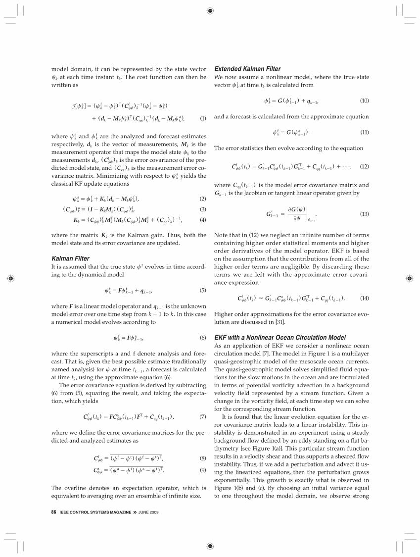
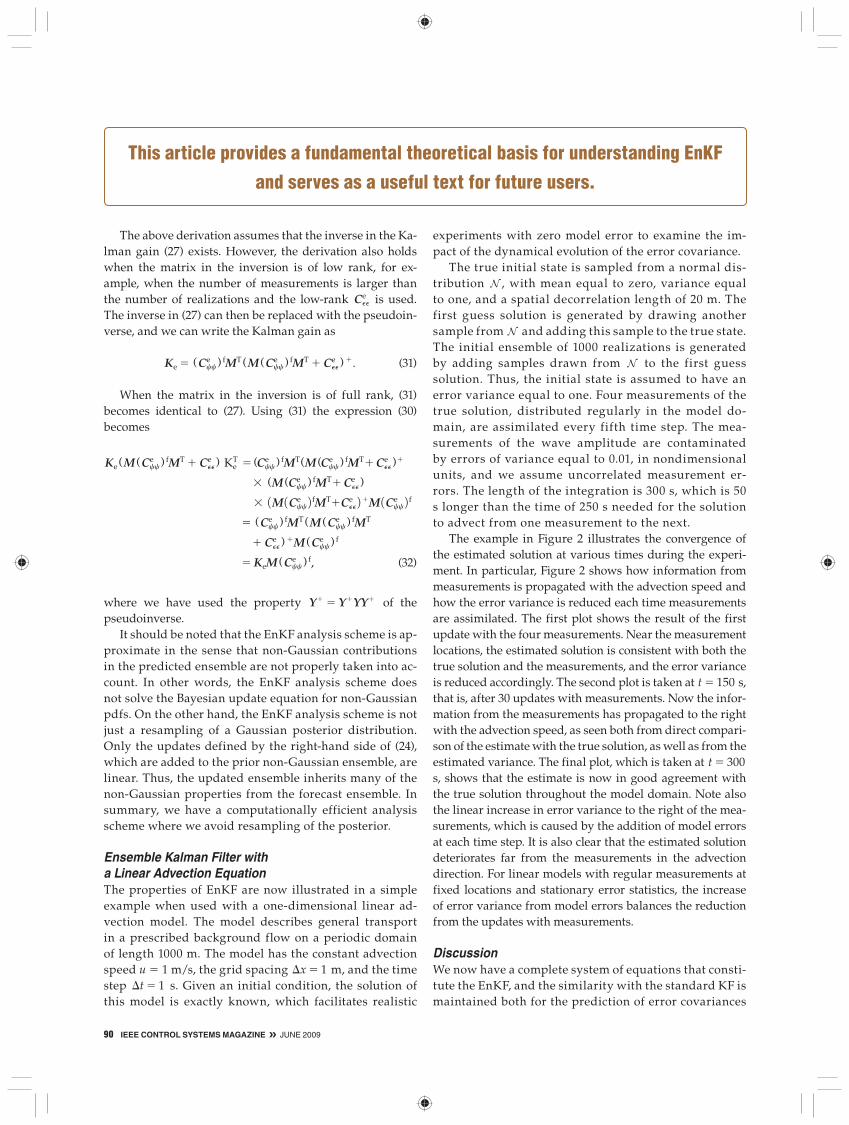
Ensemble Kalman Filter with a Linear Advection EquationThe properties of EnKF are now illustrated in a simple example when used with a one-dimensional linear ad-vection model. The model describes general transport in a prescribed background flow on a periodic domain of length 1000 m. The model has the constant advection speed u 5 1 m/s, the grid spacing Dx 5 1 m, and the time step Dt 5 1 s. Given an initial condition, the solution of this model is exactly known, which facilitates realistic
experiments with zero model error to examine the im-pact of the dynamical evolution of the error covariance.
The true initial state is sampled from a normal dis-tribution N , with mean equal to zero, variance equal to one, and a spatial decorrelation length of 20 m. The first guess solution is generated by drawing another sample from N and adding this sample to the true state. The initial ensemble of 1000 realizations is generated by adding samples drawn from N to the first guess solution. Thus, the initial state is assumed to have an error variance equal to one. Four measurements of the true solution, distributed regularly in the model do-main, are assimilated every fifth time step. The mea-surements of the wave amplitude are contaminated by errors of variance equal to 0.01, in nondimensional units, and we assume uncorrelated measurement er-rors. The length of the integration is 300 s, which is 50 s longer than the time of 250 s needed for the solution to advect from one measurement to the next.
The example in Figure 2 illustrates the convergence of the estimated solution at various times during the experi-ment. In particular, Figure 2 shows how information from measurements is propagated with the advection speed and how the error variance is reduced each time measurements are assimilated. The first plot shows the result of the first update with the four measurements. Near the measurement locations, the estimated solution is consistent with both the true solution and the measurements, and the error variance is reduced accordingly. The second plot is taken at t 5 150 s, that is, after 30 updates with measurements. Now the infor-mation from the measurements has propagated to the right with the advection speed, as seen both from direct compari-son of the estimate with the true solution, as well as from the estimated variance. The final plot, which is taken at t 5 300 s, shows that the estimate is now in good agreement with the true solution throughout the model domain. Note also the linear increase in error variance to the right of the mea-surements, which is caused by the addition of model errors at each time step. It is also clear that the estimated solution deteriorates far from the measurements in the advection direction. For linear models with regular measurements at fixed locations and stationary error statistics, the increase of error variance from model errors balances the reduction from the updates with measurements.
DiscussionWe now have a complete system of equations that consti-tute the EnKF, and the similarity with the standard KF is maintained both for the prediction of error covariances
This article provides a fundamental theoretical basis for understanding EnKF
and serves as a useful text for future users.
JUNE 2009 « IEEE CONTROL SYSTEMS MAGAZINE 91
and in the analysis scheme. For lin-ear dynamics the EnKF solution converges exactly to the KF solution with increasing ensemble size.
One of the advantages of EnKF is that, for nonlinear models, the equa-tion for the mean is solved and no closure assumption is used since each ensemble member is integrated by the full nonlinear model. This nonlinear error evolution is contrary to the ap-proximate equation for the mean (16), which is used in EKF.
Thus, it is possible to interpret EnKF as a purely statistical Monte Carlo meth-od where the ensemble of model states evolves in state space with the mean as the best estimate and the spreading of the ensemble as the error variance. At measurement times each observation is represented by another ensemble, where the mean is the actual measure-ment and the variance of the ensemble represents the measurement errors. Thus, we combine a stochastic predic-tion step with a stochastic analysis step.
PROBABILISTIC FORMULATIONFor the ensemble Kalman smoother (EnKS) [8], the estimate at a particular time is updated based on past, present, and future measurements. In contrast, a filter estimate is influenced only by the past and present measurements. Thus, EnKF becomes a special case of EnKS, where information from measurements is not projected backward in time. The assumptions of measurement errors being independent in time and the dy-namical model being a Markov process are sufficient to derive the EnKF and the EnKS. These assumptions are nor-mally not critical and are already used in the original KF. It is also possible to include the estimation of static model parameters in a consistent manner. The combined parameter and state estimation problem for a dy-namical model can be formulated as finding the joint pdf of the parameters and model state, given a set of measurements and a dynamical model with known uncertainties.
Model Equations and MeasurementsWe consider a model with associated initial and boundary conditions on the spatial domain D with boundary 'D, and with observations
'c (x,t )
't5 G (c (x, t ) , a (x ) ) 1 q (x, t ) , (33)
c (x, t0 ) 5 C0 (x ) 1 a(x ) , (34)
c (j, t ) 5 Cb(j, t ) 1 b (j, t ), for all j [ dD, (35)
a (x ) 5 a0 (x ) 1 a r (x ) , (36)
M 3c, a 45 d 1 P. (37)
The model state c (x, t ) [ Rnc is a vector consisting of the
nc model variables, where each variable is a function of
0 200 400 600Distance (Meter)
(a)
800 1000
0 200 400 600Distance (Meter)
(b)
800 1000
0 200 400 600Distance (Meter)
(c)
800 1000
0
1
2
3
4
5
6
7
Wav
e A
mpl
itude
(N
ondi
men
sion
al)
8
0
1
2
3
4
5
6
7
Wav
e A
mpl
itude
(N
ondi
men
sion
al)
8
0
1
2
3
4
5
6
7
Wav
e A
mpl
itude
(N
ondi
men
sion
al)
8MeasurementsTrue SolutionEstimated SolutionEstimated Std.Dev.
MeasurementsTrue SolutionEstimated SolutionEstimated Std.Dev.
MeasurementsTrue SolutionEstimated SolutionEstimated Std.Dev.
FIGURE 2 An ensemble Kalman fi lter experiment. For this experiment a linear advection equation illustrates how a limited ensemble size of 100 realizations facilitates estimation in a high-dimensional system whose state vector contains 1000 entries. The plots show the reference solution, measurements, estimate, and standard deviation at three different times, (a) t 5 5 s, (b) t 5 150 s, and (c) t 5 300 s.
92 IEEE CONTROL SYSTEMS MAGAZINE » JUNE 2009
space and time. The nonlinear model is defined by (33), where G (c, a ) [ R
nc is the nonlinear model operator. More general forms can be used for the nonlinear model opera-tor, although (33) suffices to demonstrate the methods con-sidered here.
The model state is assumed to evolve in time from the ini-tial state C0 (x ) [ R
nc defined in (34), under the constraints of the boundary conditions Cb(j, t ) [ R
nc defined in (35). The coordinate j runs over the surface 'D,where the bound-ary conditions are defined. The variable b is used to repre-sent errors in the boundary conditions.
We define a (x ) [ Rna as the set of na poorly known pa-
rameters of the model. The parameters can be a vector of spatial fields in the form written here, or, alternatively, a vector of scalars, and are assumed to be constant in time. A prior estimate a0 (x ) [ R
na of the vector of parameters a (x ) [ R
na is introduced through (36), and possible errors in the prior are represented by a r (x ) .
Additional conditions are present in the form of the measurements d [ R
M. Both direct point measurements of the model solution and more complex parameters that are nonlinearly related to the model state can be used. For the time being we restrict ourselves to the case of linear mea-surements. An example of a direct measurement functional is then
Mi 3c 45 33cT(x, t )dci
d ( t2 ti)d (x2 xi)dt dx5c (xi, ti)dci,
(38)
where the integration is over the space and time domain of the model. The measurement di is related to the model-state variable as selected by the vector dci
[ Rnc and evaluated at
the space and time location (xi, ti). If a model with three state variables is used and the second variable is measured, then dci
becomes the vector (0, 1, 0)T, while d ( t2 ti) and d (x2 xi) are Dirac delta functions.
In (33)–(37) we include unknown error terms, q , a , b, a r, and P, which represent errors in the model equations, the initial and boundary conditions, the first guess for the model parameters, and the measurements, respectively. Without these error terms the system as given above is overdetermined and has no solution. On the other hand,
when we introduce these error terms without additional conditions, the system has infinitely many solutions. The way to proceed is to introduce a statistical hypothesis about the errors, for example, assuming that the errors are normally distributed with means equal to zero and known error covariances.
Bayes TheoremWe now consider the model variables, the poorly known parameters, the initial and boundary conditions, and the measurements as random variables, which can be described by pdfs. The joint pdf for the model state, as a function of space, time, and the parameters, is f(c, a ) . Furthermore, for the measurements we can define the likelihood func-tion f(d|c, a ) . Thus, we may have measurements of both the model state and the parameters. Using Bayes theorem, the parameter and state estimation problem is now written in the simplified form
f(c, a|d) 5gf(c, a ) f(d|c, a ), (39)
where g is a constant of proportionality whose computa-tion requires the evaluation of the integral of (39) over the high-dimensional solution and parameter space.
Parameter estimation problems, in particular, for ap-plications involving high-dimensional models, such as oceanic, atmospheric, marine ecosystem, hydrology, and petroleum applications, often do not include the model state as a variable to be estimated. It is more common to first solve for the poorly known parameters by minimizing an appropriate cost function where the model equations act as a strong constraint and then rerun the model to find the model solution. It is then implicitly assumed that the model does not contain errors, an assumption that gener-ally is invalid.
In the dynamical model, we specify initial and bound-ary conditions as random variables, and we include prior information about the parameters. Thus, we define the pdfs f(c0 ) , f(cb) , and f(a ) for the estimates c0, cb , and a of the initial and boundary conditions, and the parameters, respectively. Instead of f(c,a ) , we write
f(c, a, c0, cb) 5 f(c|a, c0, cb) f(c0 ) f(cb) f(a ) . (40)
Equation (39) should accordingly be written as
f(c, a, c0, cb|d)5gf(c|a, c0, cb) f(c0 ) f(cb) f(a ) f(d|c, a ), (41)
where it is also assumed that the boundary conditions and initial conditions are independent, although this as-sumption may not be true for the locations where initial and boundary conditions intersect at t0. Here the pdf f(c|a, c0, cb) is the prior density for the model solution given the parameters and initial and boundary conditions.
t0 t1 t2 t3 t4 t5 t6 t7 ti tkψ0 ψ1 ψ2 ψ3 ψ4 ψ5 ψ6 ψ7 ψi ψk
dJd2 d3d1ti(1) ti(2) ti(3) ti(j) t i(J)
dj
. . .
. . .
. . .. . .. . . . . .
. . .
. . .
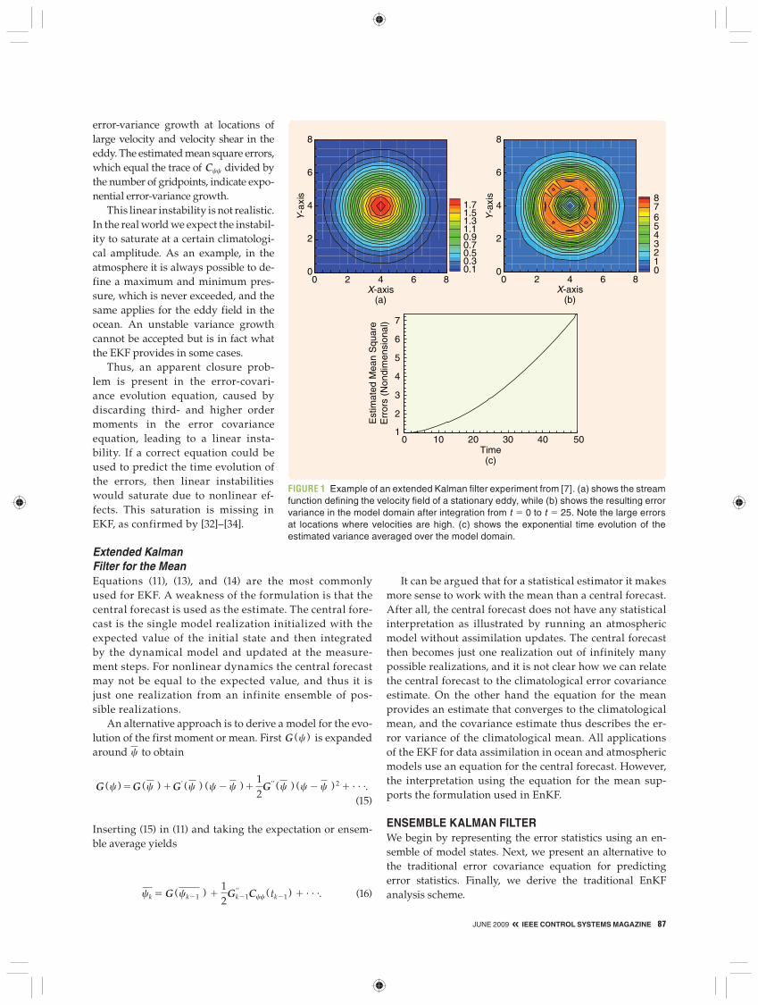
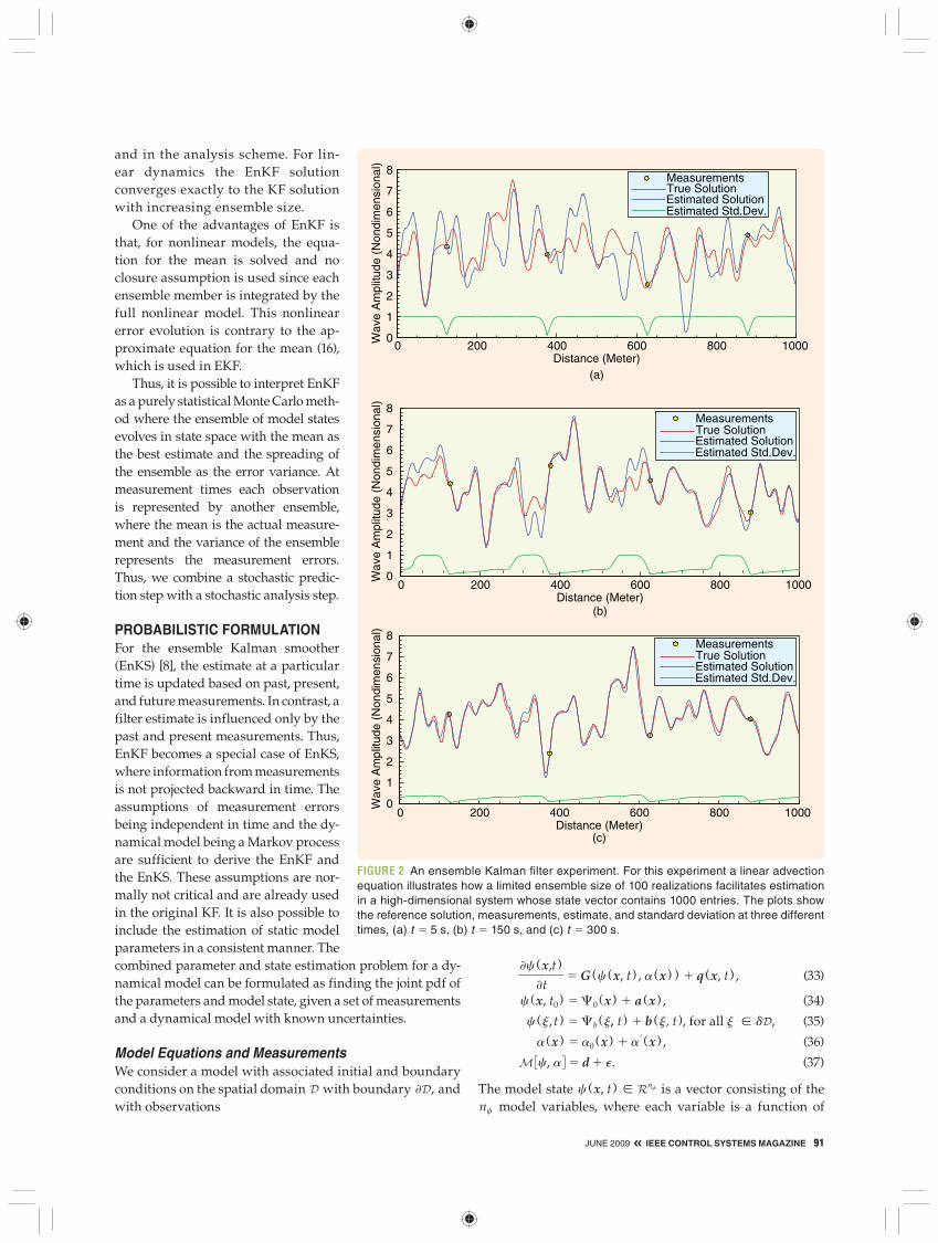
FIGURE 3 Discretization in time. The time interval is discretized into k1 1 nodes, t 0 to t k, where the model state vector ci 5c 1 ti 2 is defined. The measurement vectors dj are available at the discrete subset of times t i 1j2, where j5 1, . . . , j.
JUNE 2009 « IEEE CONTROL SYSTEMS MAGAZINE 93
Discrete Formulation
In the following discussion we work with a model state that is discretized in time, that is, c (x, t ) is represented at fixed time intervals as ci(x ) 5c (x, ti) with i5 0, 1, c, k ; see Figure 3. Furthermore, we define the pdf for the model in-tegration from time ti21 to ti as f(ci|ci21, a, cb( ti) ) , which assumes that the model is a first-order Markov process. The joint pdf for the model solution and the parameters in (40) can now be written as
f(c1, c, ck, a, c0, cb)
5 f(a ) f(cb) f(c0 ) qk
i51f(ci|ci21, a, cb) . (42)
Independent MeasurementsWe now assume that the measurements d [ R
M can be divided into subsets of measurement vectors dj [ R
mj, collected at times ti(j) , with j5 1, c, J and 0 , i(1) , i(2) ,c, i( J ) , k. The subset dj depends only on c ( ti(j) ) 5ci(j) and a. Further-more, it is assumed that the measurement errors are uncorre-lated in time. We can then write
f(d|c, a ) 5qJ
j51f(dj|ci(j), a ) , (43)
and from Bayes theorem we obtain
f(c1, c, ck, a, c0, cb|d)
5gf(a ) f(c0 ) f(cb) qk
i51f(ci|ci21, a ) q
J
j51f(dj|ci(j), a ) . (44)
Sequential Processing of MeasurementsIt is shown in [36] and [37] that, in the case of time- correlated model errors, it is possible to reformulate the problem as a first-order Markov process by augmenting the model er-rors to the model-state vector. A simple equation forced by white noise can be used to simulate the time evolution of the model errors.
In [38] it is shown that a general smoother and filter can be derived from the Bayesian formulation given in (44). We now rewrite (44) as a sequence of iterations
f(c1, c, ci(j), a, c0, cb|d1, c, dj)
5gf(c1, c, ci(j21), a, c0, cb|d1, c, dj21 )
3 qi(j)
i5i(j21)11f(ci|ci21, a ) f(dj|ci(j), a ) . (45)
Thus, we formulate the combined parameter and state- estimation problem using Bayesian statistics and see that, under the condition that measurement errors are indepen-dent in time and the dynamical model is a Markov process, a recursive formulation can be used for Bayes theorem.
That is, the model state and parameters with their respec-tive uncertainties are updated sequentially in time when-ever the measurements become available.
We note again that this recursion does not introduce any significant approximations and thus describes the full inverse problem as long as the model is a Markov process and the measurements errors are independent in time. Further, for many problems the recursive processing of measurements provides a better posed approach for solv-ing the inverse problem than trying to process all of the measurements simultaneously as is normally done in vari-ational formulations. Sequential processing is also conve-nient for forecasting problems where new measurements can be processed when they arrive without recomputing the full inversion.
Ensemble SmootherThe ensemble smoother (ES) can be derived by assuming that the pdfs for the model prediction as well as the likeli-hood are Gaussian and by using the original Bayes theo-rem (41). The derivation requires that we approximate the pdfs resulting from an integration of the ensemble through the whole assimilation time period with Gauss-ian pdfs. We can then replace Bayes theorem with a least squares cost function similar to (1), but with the time di-mension included, and the analysis becomes a standard variance minimizing analysis in space and time. All of the data are processed in one step, and the solution is up-dated as a function of space and time, using the space-time covariances estimated from the ensemble of model realizations. The ES in [39] is computed as a first-guess estimate, which is the mean of the freely evolving ensem-ble, plus a linear combination of time-dependent influ-ence functions, which are calculated from the ensemble statistics. Thus, the method is equivalent to a variance-minimizing objective analysis method where the time dimension is included.
Ensemble Kalman SmootherAn assumption of Gaussian pdfs for the model prediction (the prior) and the distribution for the data (the likeli-hood function) in (45) allows us to replace the Bayesian update formula with a least squares cost function sim-ilar to (1) but additionally including the state vector at all previous times. Again the cost function is minimized using a standard variance-minimizing analysis scheme, involving a state variable defined from the initial time to the current update time. That is, we also update the state variables backward in time using the combined time and space ensemble covariances. This scheme results in the EnKS as in [38].
Ensemble Kalman FilterThe EnKF is just a special case of EnKS where the up-dates at previous times are skipped. EnKF is obtained by
94 IEEE CONTROL SYSTEMS MAGAZINE » JUNE 2009
integrating out the state variables at all previous times from (45) and assuming that the resulting model pdf for the current time as well as the likelihood function are Gaussian. The incremental update (45) can then be re-placed by the penalty function (1), leading to the standard Kalman filter analysis equations. Thus, the measurements are filtered. At the final time, or, actually, from the lat-est update and for predictions into the future, EnKF and EnKS provide identical solutions.
EXAMPLE WITH THE LORENZ EQUATIONSThe example from [40] and [38] with the chaotic Lorenz model of [41] is now used to compare ES, EnKS, and EnKF. The Lorenz model consists of the coupled system of nonlin-ear ordinary differential equations given by
dxdt
5 g (y 2 x ) , (46)
dy
dt5 rx 2 y 2 xz, (47)
dzdt
5 xy 2 bz. (48)
Here x ( t ), y ( t ), and z ( t ) are the dependent variables, and we choose the parameter values g 5 10, r 5 28, and b 5 8/3. The initial conditions for the reference case are
given by (x0, y0, z0 ) 5 (1.508870, 2 1.531271, 25.46091) and the time interval is t [ 30, 40 4 .
The observations and initial conditions are simulated by adding normally distributed white noise with zero mean and variance equal to 2.0 to the reference solution. All of the variables x , y , and z are measured. In the calculation of the ensemble statistics, an ensemble of 1000 members is used. The same simulation is rerun with various ensemble sizes, and the differences between the results are negligible with as few as 50 ensemble members.
The three methods discussed above are now exam-ined and compared in an experiment where the time between measurements is Dtobs 5 0.5 , which is similar to Experiment B in [40]. In the upper plots in figures 4–6, the red line denotes the estimate and the blue line is the reference solution. In the lower plots the red line is the standard deviation estimated from ensemble statistics, while the blue line is the true residuals with respect to the reference solution.
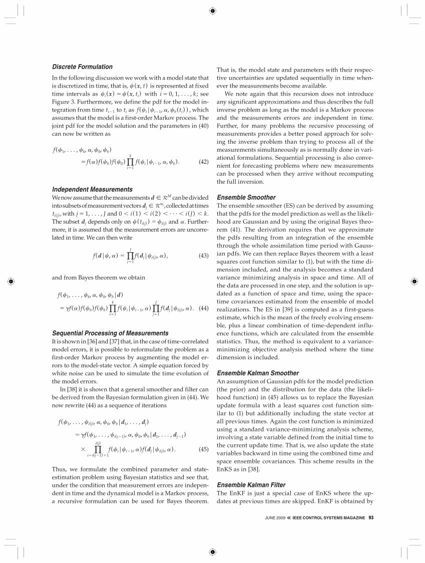
Ensemble Smoother SolutionThe ES solution for the x-component and the associated estimated error variance are given in Figure 4. It is found that the ES performs rather poorly with the current data density. Note, however, that even if the fit to the reference trajectory is poor, the ES solution captures most of the tran-sitions. The main problem is related to the estimate of the amplitudes in the reference solution. The problem is linked to the appearance of non-Gaussian contributions in the dis-tribution for the model evolution, which can be expected in such a strongly nonlinear case.
Clearly, the error estimates evaluated from the pos-terior ensemble are not large enough at the peaks where the smoother performs poorly. The underestimated errors again result from neglecting the non-Gaussian contribution from the probability distribution for the model evolution. Otherwise, the error estimate looks reasonable with mini-ma at the measurement locations and maxima between the measurements. Note again that if a linear model is used, then the posterior density becomes Gaussian and the ES provides, in the limit of an infinite ensemble size, the same solution as the EnKS and the Kalman smoother.
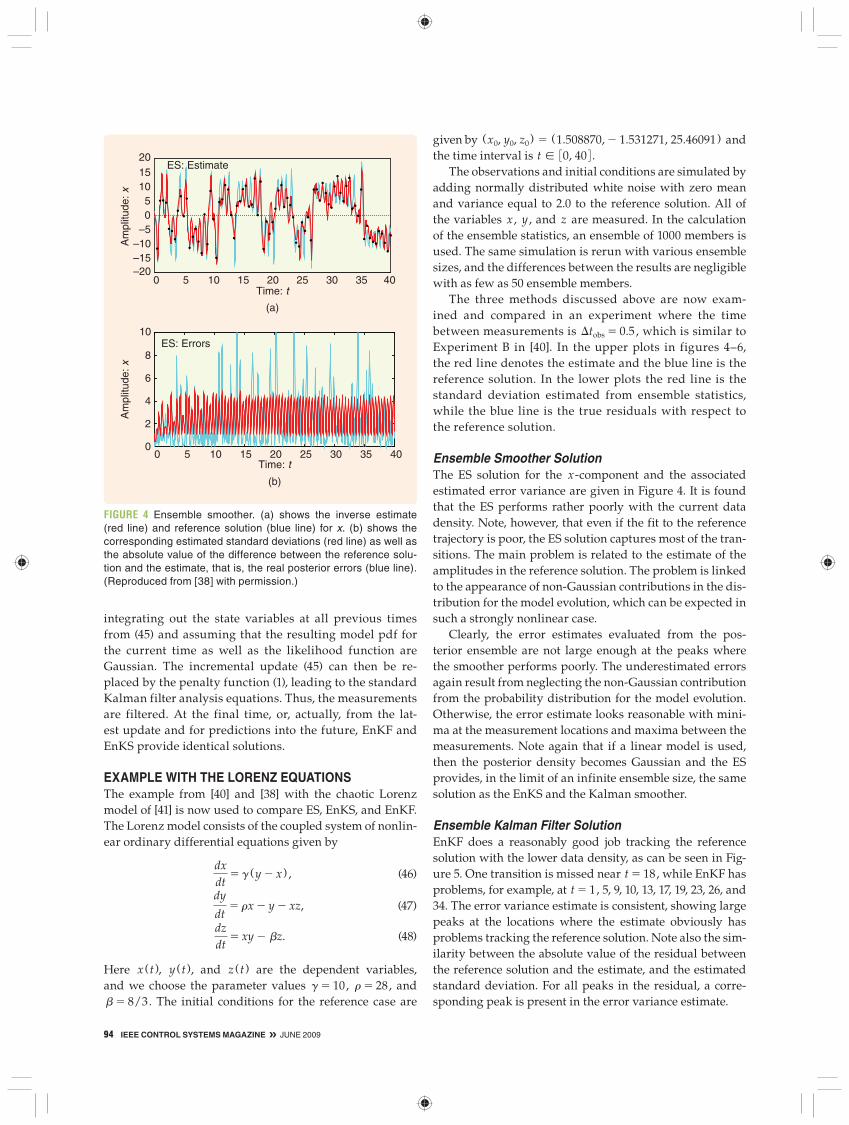
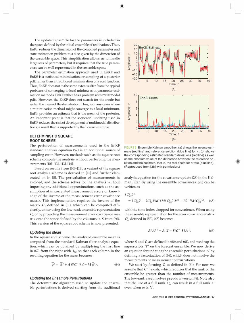
Ensemble Kalman Filter Solution EnKF does a reasonably good job tracking the reference solution with the lower data density, as can be seen in Fig-ure 5. One transition is missed near t 5 18, while EnKF has problems, for example, at t 5 1, 5, 9, 10, 13, 17, 19, 23, 26, and 34. The error variance estimate is consistent, showing large peaks at the locations where the estimate obviously has problems tracking the reference solution. Note also the sim-ilarity between the absolute value of the residual between the reference solution and the estimate, and the estimated standard deviation. For all peaks in the residual, a corre-sponding peak is present in the error variance estimate.
–20–15–10–505
101520
0 5 10 15 20 25 30 35 40
Am
plitu
de: x
Time: t
(a)
Time: t
(b)
ES: Estimate
0
2
4
6
8
10
0 5 10 15 20 25 30 35 40
Am
plitu
de: x
ES: Errors
FIGURE 4 Ensemble smoother. (a) shows the inverse estimate (red line) and reference solution (blue line) for x. (b) shows the corresponding estimated standard deviations (red line) as well as the absolute value of the difference between the reference solu-tion and the estimate, that is, the real posterior errors (blue line). (Reproduced from [38] with permission.)
JUNE 2009 « IEEE CONTROL SYSTEMS MAGAZINE 95
The error estimates show the same behavior as in [32] with very strong error growth when the model solution passes through the unstable regions of the state space and otherwise weak error variance growth or even decay in the stable regions. Note, for example, the low error variance for t [ 328, 34 4 corresponding to the oscillation of the solution around one of the attractors.
In this case, the nonlinearity of the problem causes EnKF to perform better than the ES. In fact, at each up-date, the realizations are pulled toward the true solution and are not allowed to diverge toward the wrong attrac-tors of the system. In addition, the Gaussian increments of the ensemble members lead to an approximately Gaussian ensemble distributed around the true solution. This property of the sequential updating is not exploited in the ES, where realizations evolve freely and lead to non-Gaussian ensemble distributions. Note again that if the model dynamics are linear, then, in the limit of an infinite ensemble size, EnKF gives the same solution as the Kalman filter and the ES solution gives a better result than EnKF.
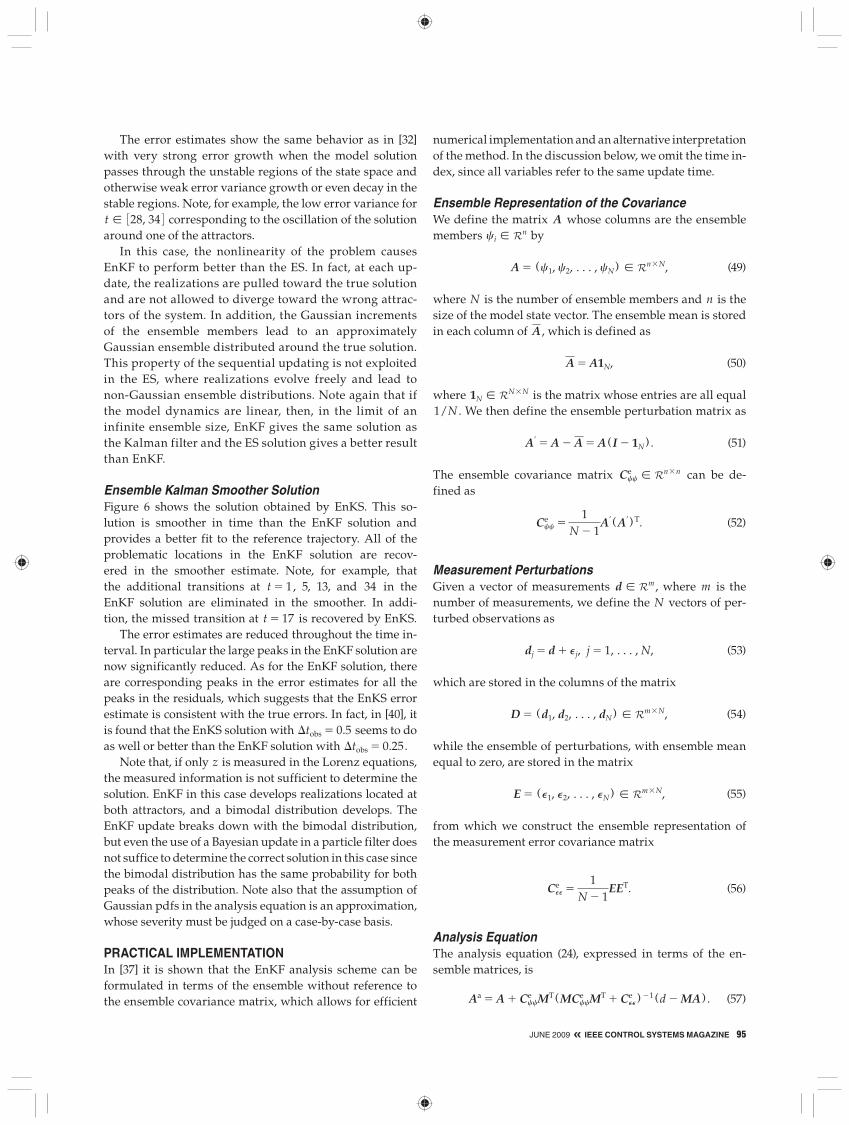
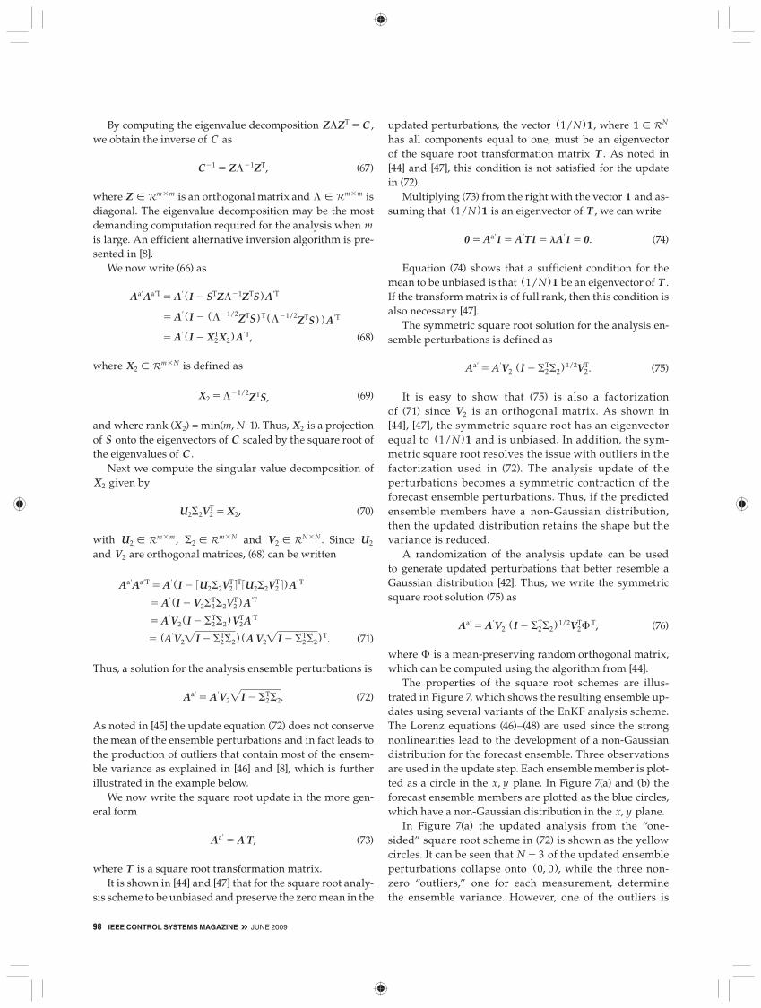
Ensemble Kalman Smoother Solution Figure 6 shows the solution obtained by EnKS. This so-lution is smoother in time than the EnKF solution and provides a better fit to the reference trajectory. All of the problematic locations in the EnKF solution are recov-ered in the smoother estimate. Note, for example, that the additional transitions at t 5 1, 5, 13, and 34 in the EnKF solution are eliminated in the smoother. In addi-tion, the missed transition at t 5 17 is recovered by EnKS.
The error estimates are reduced throughout the time in-terval. In particular the large peaks in the EnKF solution are now significantly reduced. As for the EnKF solution, there are corresponding peaks in the error estimates for all the peaks in the residuals, which suggests that the EnKS error estimate is consistent with the true errors. In fact, in [40], it is found that the EnKS solution with Dtobs 5 0.5 seems to do as well or better than the EnKF solution with Dtobs 5 0.25.
Note that, if only z is measured in the Lorenz equations, the measured information is not sufficient to determine the solution. EnKF in this case develops realizations located at both attractors, and a bimodal distribution develops. The EnKF update breaks down with the bimodal distribution, but even the use of a Bayesian update in a particle filter does not suffice to determine the correct solution in this case since the bimodal distribution has the same probability for both peaks of the distribution. Note also that the assumption of Gaussian pdfs in the analysis equation is an approximation, whose severity must be judged on a case-by-case basis.
PRACTICAL IMPLEMENTATIONIn [37] it is shown that the EnKF analysis scheme can be formulated in terms of the ensemble without reference to the ensemble covariance matrix, which allows for efficient
numerical implementation and an alternative interpretation of the method. In the discussion below, we omit the time in-dex, since all variables refer to the same update time.
Ensemble Representation of the CovarianceWe define the matrix A whose columns are the ensemble members ci [ R
n by
A 5 (c1, c2, c, cN) [ Rn3N, (49)
where N is the number of ensemble members and n is the size of the model state vector. The ensemble mean is stored in each column of A , which is defined as
A 5 A1N, (50)
where 1N [ RN3N is the matrix whose entries are all equal
1/N . We then define the ensemble perturbation matrix as
Ar 5 A 2 A 5 A (I 2 1N) . (51)
The ensemble covariance matrix Ccce [ R
n3n can be de-fined as
Ccce 5
1N 2 1
Ar (Ar )T. (52)
Measurement PerturbationsGiven a vector of measurements d [ R
m , where m is the number of measurements, we define the N vectors of per-turbed observations as
dj 5 d 1 Pj, j 5 1, c, N, (53)
which are stored in the columns of the matrix
D 5 (d1, d2, c, dN) [ Rm3N, (54)
while the ensemble of perturbations, with ensemble mean equal to zero, are stored in the matrix
E 5 (P1, P2, c, PN) [ Rm3N, (55)
from which we construct the ensemble representation of the measurement error covariance matrix
CPPe 5
1N 2 1
EET. (56)
Analysis EquationThe analysis equation (24), expressed in terms of the en-semble matrices, is
Aa 5 A 1 Ccce MT(MCcc
e MT 1 CPPe ) 21 (d 2 MA ) . (57)
96 IEEE CONTROL SYSTEMS MAGAZINE » JUNE 2009
Using the ensemble of innovation vectors defined as
Dr 5 D 2 MA, (58)
along with the definitions of the ensemble error cova-riance matrices in (52) and (56), the analysis can be ex-pressed as
Aa 5 A 1 ArArTMT(MArArTMT 1 EET) 21Dr, (59)
where all references to the error covariance matrices are eliminated.
We now introduce the matrix S [ Rm3N holding the
measurements of the ensemble perturbations by
S 5 MAr, (60)
and the matrix C [ Rm3m ,
C 5 SST 1 (N 2 1)CPP. (61)
Here we can use the full-rank, exact measurement error co-variance matrix CPP as well as the low-rank representation CPP
e defined in (56).
The analysis equation (59) can then be written as
Aa 5 A 1 ArSTC21Dr 5 A 1 A (I 2 1N)STC21Dr 5 A (I 1 (I 2 1N)STC21Dr ) 5 A (I 1 STC21Dr ) 5 AX, (62)
where we use (51) and 1NST ; 0 . The matrix X [ RN3N is
defined as
X 5 I 1 STC21Dr. (63)
Thus, the EnKF analysis becomes a combination of the fore-cast ensemble members and is searched for in the space spanned by the forecast ensemble.
It is clear that (62) is a stochastic scheme due to the use of randomly perturbed measurements. Thus, (62) allows for a nice interpretation of EnKF as a sequential Markov chain Monte Carlo algorithm, while making it easy to un-derstand and implement the method. The efficient and stable numerical implementation of the analysis scheme is discussed in [8], including the case in which C is singular due to the number of measurements being larger than the number of realizations.
In practice, the ensemble size is critical since the com-putational cost scales linearly with the number of real-izations. That is, each individual realization needs to be integrated forward in time. The cost associated with the ensemble integration motivates the use of an ensemble with the minimum number of realizations that can pro-vide acceptable accuracy.
There are two major sources of sampling errors in EnKF, namely, the use of a finite ensemble of stochastic model re-alizations as well as the introduction of stochastic measure-ment perturbations [8], [42]. In addition, stochastic model errors influence the predicted error statistics, which is ap-proximated by the ensemble. The sampling of physically acceptable model realizations and realizations of model er-rors is chosen to ensure that the ensemble matrix has full rank and good conditioning. Furthermore, stochastic per-turbation of measurements used in EnKF can be avoided using a square root implementation of the analysis scheme, to be discussed below.
EnKF for Combined Parameter and State EstimationWhen using EnKF to estimate poorly known model parameters, we start by representing the prior pdfs of the parameters by an ensemble of realizations, which is aug-mented to the state ensemble matrix A at the update steps. The poorly known parameters are then updated using the variance-minimizing analysis scheme, where the covari-ances between the predicted data and the parameters are used to update the parameters.
–20–15–10–505
1015
20
Am
plitu
de: x
EnKF: Estimate
0
2
4
6
8
10
0 5 10 15 20 25 30 35 40
Am
plitu
de: x
Time: t
(b)
0 5 10 15 20 25 30 35 40Time: t
(a)
EnKF: Errors
FIGURE 5 Ensemble Kalman filter. (a) shows the inverse estimate (red line) and reference solution (blue line) for x . (b) shows the corresponding estimated standard deviations (red line) as well as the absolute value of the difference between the reference solu-tion and the estimate, that is, the real posterior errors (blue line). (Reproduced from [38] with permission.)
JUNE 2009 « IEEE CONTROL SYSTEMS MAGAZINE 97
The updated ensemble for the parameters is included in the space defined by the initial ensemble of realizations. Thus, EnKF reduces the dimension of the combined parameter and state estimation problem to a size given by the dimension of the ensemble space. This simplification allows us to handle large sets of parameters, but it requires that the true param-eters can be well represented in the ensemble space.
The parameter estimation approach used in EnKF and EnKS is a statistical minimization, or sampling of a posterior pdf, rather than a traditional minimization of a cost function. Thus, EnKF does not to the same extent suffer from the typical problems of converging to local minima as in parameter-esti-mation methods. EnKF rather has a problem with multimodal pdfs. However, the EnKF does not search for the mode but rather the mean of the distribution. Thus, in many cases where a minimization method might converge to a local minimum, EnKF provides an estimate that is the mean of the posterior. An important point is that the sequential updating used in EnKF reduces the risk of development of multimodal distribu-tions, a result that is supported by the Lorenz example.
DETERMINISTIC SQUARE ROOT SCHEMEThe perturbation of measurements used in the EnKF standard analysis equation (57) is an additional source of sampling error. However, methods such as the square root scheme compute the analysis without perturbing the mea-surements [10]–[13], [43], [44].
Based on results from [10]–[13], a variant of the square root analysis scheme is derived in [42] and further elab-orated on in [8]. The perturbation of measurements is avoided, and the scheme solves for the analysis without imposing any additional approximations, such as the as-sumption of uncorrelated measurement errors or knowl-edge of the inverse of the measurement error covariance matrix. This implementation requires the inverse of the matrix C , defined in (61), which can be computed effi-ciently, either using the low-rank ensemble representation Ce or by projecting the measurement error covariance ma-trix onto the space defined by the columns in S from (60). This version of the square root scheme is now presented.
Updating the MeanIn the square root scheme, the analyzed ensemble mean is computed from the standard Kalman filter analysis equa-tion, which can be obtained by multiplying the first line in (62) from the right with 1N , so that each column in the resulting equation for the mean becomes
ca 5 c f 1 ArSTC21 (d 2 M c f ) . (64)
Updating the Ensemble PerturbationsThe deterministic algorithm used to update the ensem-ble perturbations is derived starting from the traditional
analysis equation for the covariance update (28) in the Kal-man filter. By using the ensemble covariances, (28) can be written as
(Ccce ) a
5 (Ccce ) f 2 (Ccc
e ) fMT(M (Ccce ) fMT 1 R ) 21M (Ccc
e ) f, (65)
with the time index dropped for convenience. When using the ensemble representation for the error covariance matrix CPP
e defined in (52), (65) becomes
AarAarT 5 Ar (I 2 STC21S)ArT, (66)
where S and C are defined in (60) and (61), and we drop the superscripts “f” on the forecast ensemble. We now derive an equation for updating the ensemble perturbations Ar by defining a factorization of (66), which does not involve the measurements or measurement perturbations.
We start by forming C as defined in (61). For now we assume that C21 exists, which requires that the rank of the ensemble be greater than the number of measurements. The low-rank case involves pseudo inversion [8]. Note also that the use of a full rank CPP
e can result in a full rank C even when m $ N .
–20–15–10–505
1015
20
Am
plitu
de: x
EnKS: Estimate
0
2
4
6
8
10
0 5 10 15 20 25 30 35 40A
mpl
itude
: x
Time: t
(b)
0 5 10 15 20 25 30 35 40Time: t
(a)
EnKS: Errors
FIGURE 6 Ensemble Kalman smoother. (a) shows the inverse esti-mate (red line) and reference solution (blue line) for x . (b) shows the corresponding estimated standard deviations (red line) as well as the absolute value of the difference between the reference so-lution and the estimate, that is, the real posterior errors (blue line). (Reproduced from [38] with permission.)
98 IEEE CONTROL SYSTEMS MAGAZINE » JUNE 2009
By computing the eigenvalue decomposition ZLZT 5 C , we obtain the inverse of C as
C21 5 ZL21ZT, (67)
where Z [ Rm3m is an orthogonal matrix and L [ R
m3m is diagonal. The eigenvalue decomposition may be the most demanding computation required for the analysis when m is large. An efficient alternative inversion algorithm is pre-sented in [8].
We now write (66) as
AarAarT 5 Ar (I 2 STZL21ZTS)ArT
5 Ar (I 2 (L21/2ZTS)T(L21/2ZTS) )ArT
5 Ar (I 2 X2TX2 )ArT, (68)
where X2 [ Rm3N is defined as
X2 5 L21/2ZTS, (69)
and where rank (X2) = min(m, N–1). Thus, X2 is a projection of S onto the eigenvectors of C scaled by the square root of the eigenvalues of C .
Next we compute the singular value decomposition of X2 given by
U2S2V2T 5 X2, (70)
with U2 [ Rm3m , S2 [ R
m3N and V2 [ RN3N . Since U2
and V2 are orthogonal matrices, (68) can be written
AarAarT 5 Ar (I 2 3U2S2V2T 4T 3U2S2V2
T 4 )ArT
5 Ar (I 2 V2S2TS2V2
T)ArT
5 ArV2 (I 2 S2TS2 )V2
TArT
5 (ArV2"I 2 S2TS2 ) (ArV2"I 2 S2
TS2 )T. (71)
Thus, a solution for the analysis ensemble perturbations is
Aar 5 ArV2"I 2 S2TS2. (72)
As noted in [45] the update equation (72) does not conserve the mean of the ensemble perturbations and in fact leads to the production of outliers that contain most of the ensem-ble variance as explained in [46] and [8], which is further illustrated in the example below.
We now write the square root update in the more gen-eral form
Aar 5 ArT, (73)
where T is a square root transformation matrix. It is shown in [44] and [47] that for the square root analy-
sis scheme to be unbiased and preserve the zero mean in the
updated perturbations, the vector (1/N )1 , where 1 [ RN
has all components equal to one, must be an eigenvector of the square root transformation matrix T . As noted in [44] and [47], this condition is not satisfied for the update in (72).
Multiplying (73) from the right with the vector 1 and as-suming that (1/N )1 is an eigenvector of T , we can write
0 5 Aar1 5 ArT1 5 lAr1 5 0. (74)
Equation (74) shows that a sufficient condition for the mean to be unbiased is that (1/N )1 be an eigenvector of T . If the transform matrix is of full rank, then this condition is also necessary [47].
The symmetric square root solution for the analysis en-semble perturbations is defined as
Aar 5 ArV2 (I 2 S2TS2 ) 1/2V2
T. (75)
It is easy to show that (75) is also a factorization of (71) since V2 is an orthogonal matrix. As shown in [44], [47], the symmetric square root has an eigenvector equal to (1/N )1 and is unbiased. In addition, the sym-metric square root resolves the issue with outliers in the factorization used in (72). The analysis update of the perturbations becomes a symmetric contraction of the forecast ensemble perturbations. Thus, if the predicted ensemble members have a non-Gaussian distribution, then the updated distribution retains the shape but the variance is reduced.
A randomization of the analysis update can be used to generate updated perturbations that better resemble a Gaussian distribution [42]. Thus, we write the symmetric square root solution (75) as
Aar 5 ArV2 (I 2 S2TS2 ) 1/2V2
TF T, (76)
where F is a mean-preserving random orthogonal matrix, which can be computed using the algorithm from [44].
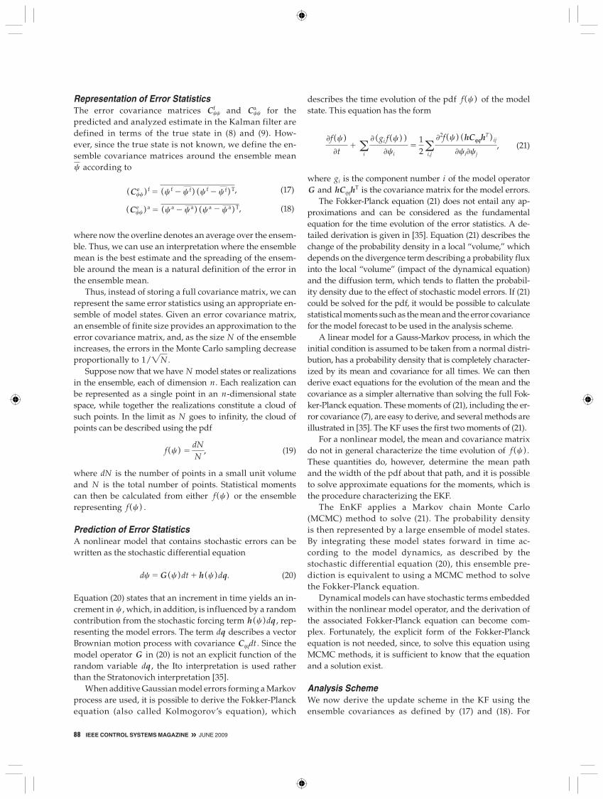
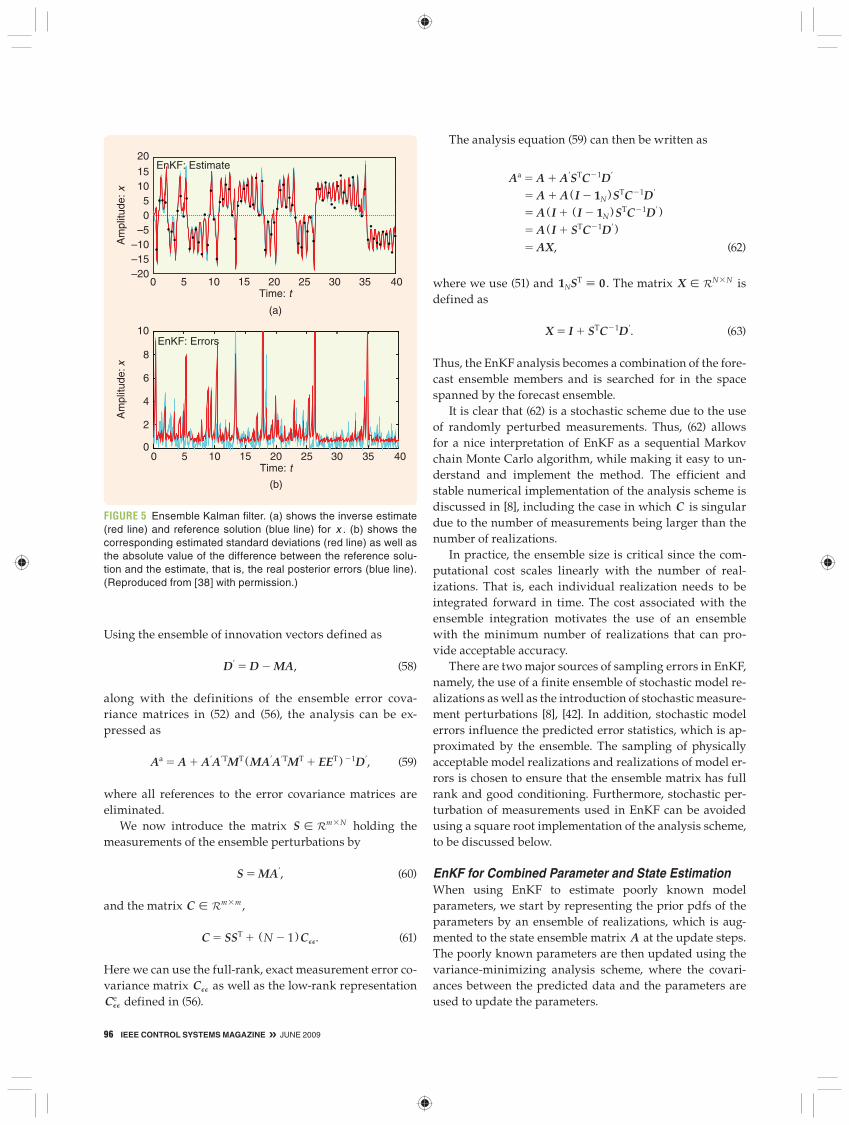
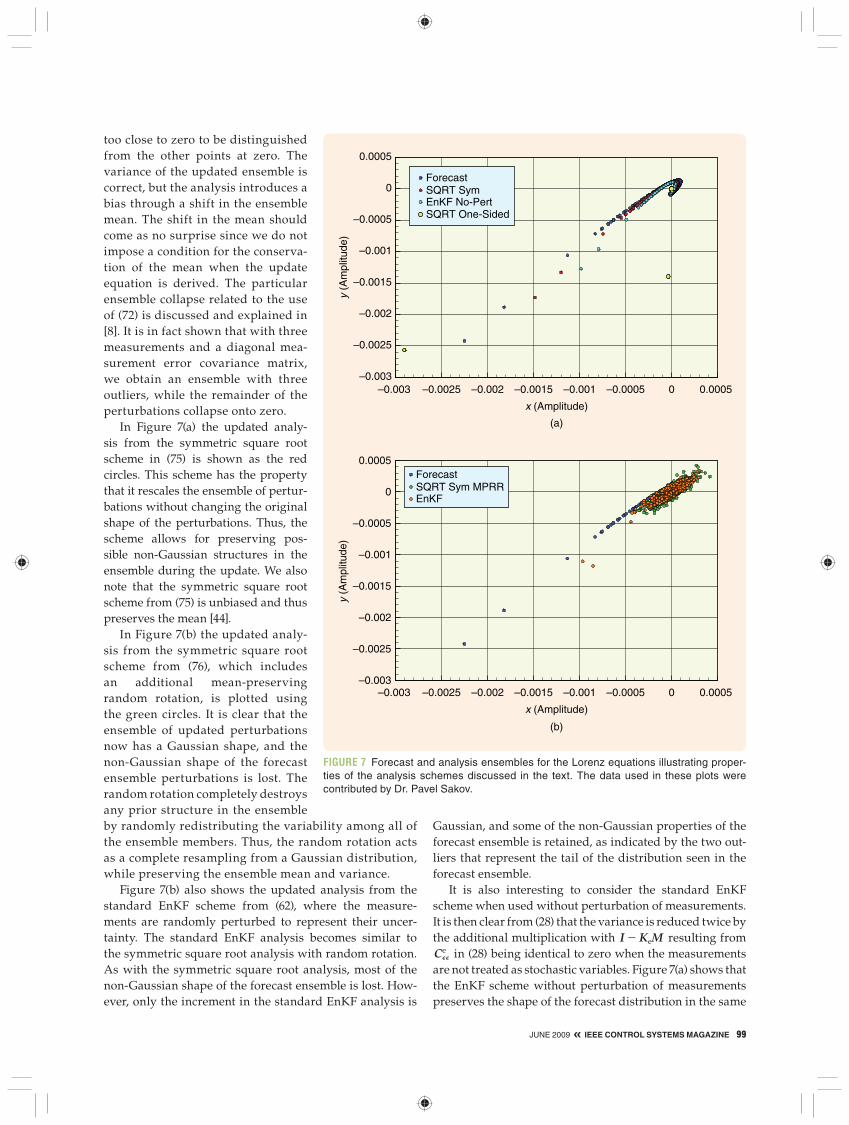
The properties of the square root schemes are illus-trated in Figure 7, which shows the resulting ensemble up-dates using several variants of the EnKF analysis scheme. The Lorenz equations (46)–(48) are used since the strong nonlinearities lead to the development of a non-Gaussian distribution for the forecast ensemble. Three observations are used in the update step. Each ensemble member is plot-ted as a circle in the x, y plane. In Figure 7(a) and (b) the forecast ensemble members are plotted as the blue circles, which have a non-Gaussian distribution in the x, y plane.
In Figure 7(a) the updated analysis from the “one-sided” square root scheme in (72) is shown as the yellow circles. It can be seen that N 2 3 of the updated ensemble perturbations collapse onto (0, 0), while the three non-zero “outliers,” one for each measurement, determine the ensemble variance. However, one of the outliers is
JUNE 2009 « IEEE CONTROL SYSTEMS MAGAZINE 99
too close to zero to be distinguished from the other points at zero. The variance of the updated ensemble is correct, but the analysis introduces a bias through a shift in the ensemble mean. The shift in the mean should come as no surprise since we do not impose a condition for the conserva-tion of the mean when the update equation is derived. The particular ensemble collapse related to the use of (72) is discussed and explained in [8]. It is in fact shown that with three measurements and a diagonal mea-surement error covariance matrix, we obtain an ensemble with three outliers, while the remainder of the perturbations collapse onto zero.
In Figure 7(a) the updated analy-sis from the symmetric square root scheme in (75) is shown as the red circles. This scheme has the property that it rescales the ensemble of pertur-bations without changing the original shape of the perturbations. Thus, the scheme allows for preserving pos-sible non-Gaussian structures in the ensemble during the update. We also note that the symmetric square root scheme from (75) is unbiased and thus preserves the mean [44].
In Figure 7(b) the updated analy-sis from the symmetric square root scheme from (76), which includes an additional mean-preserving random rotation, is plotted using the green circles. It is clear that the ensemble of updated perturbations now has a Gaussian shape, and the non- Gaussian shape of the forecast ensemble perturbations is lost. The random rotation completely destroys any prior structure in the ensemble by randomly redistributing the variability among all of the ensemble members. Thus, the random rotation acts as a complete resampling from a Gaussian distribution, while preserving the ensemble mean and variance.
Figure 7(b) also shows the updated analysis from the standard EnKF scheme from (62), where the measure-ments are randomly perturbed to represent their uncer-tainty. The standard EnKF analysis becomes similar to the symmetric square root analysis with random rotation. As with the symmetric square root analysis, most of the non-Gaussian shape of the forecast ensemble is lost. How-ever, only the increment in the standard EnKF analysis is
Gaussian, and some of the non-Gaussian properties of the forecast ensemble is retained, as indicated by the two out-liers that represent the tail of the distribution seen in the forecast ensemble.
It is also interesting to consider the standard EnKF scheme when used without perturbation of measurements. It is then clear from (28) that the variance is reduced twice by the additional multiplication with I 2 KeM resulting from CPP
e in (28) being identical to zero when the measurements are not treated as stochastic variables. Figure 7(a) shows that the EnKF scheme without perturbation of measurements preserves the shape of the forecast distribution in the same
x (Amplitude)
(a)
(b)
y (A
mpl
itude
)
–0.003 –0.0025 –0.002 –0.0015 –0.001 –0.0005 0 0.0005
x (Amplitude)
–0.003 –0.0025 –0.002 –0.0015 –0.001 –0.0005 0 0.0005
–0.003
–0.0025
–0.002
–0.0015
–0.001
–0.0005
0
0.0005
y (A
mpl
itude
)
–0.003
–0.0025
–0.002
–0.0015
–0.001
–0.0005
0
0.0005
ForecastSQRT SymEnKF No-PertSQRT One-Sided
ForecastSQRT Sym MPRREnKF
FIGURE 7 Forecast and analysis ensembles for the Lorenz equations illustrating proper-ties of the analysis schemes discussed in the text. The data used in these plots were contributed by Dr. Pavel Sakov.
100 IEEE CONTROL SYSTEMS MAGAZINE » JUNE 2009
way as the symmetric square root scheme, although the variance is too low. Thus, the perturbation of measure-ments in EnKF both increases the ensemble variance to the “correct” value, and introduces additional randomization. The randomization is different from the one observed in (76) since only the increments are randomized in the EnKF scheme with perturbation of measurements.
It is currently not clear which of the analysis schemes, that is, the standard EnKF (62), the symmetric square root (75), or the symmetric square root with random rotation (76), is best in practice. Probably the choice of analysis scheme depends on the dynamical model and possibly also on the measurement density and ensemble size used. For a linear dynamical model, the forecast distribution is Gauss-ian, and the random rotation is not needed. Thus, we then expect the symmetric square root (75) to be the best choice. On the other hand, for a strongly nonlinear dynamical model where non-Gaussian effects are dominant in the pre-dicted ensemble, the symmetric square root with a random rotation (76) or EnKF with perturbed measurements (62) may work better. Both of these schemes introduce Gaussi-anity into the analysis update, while a Gaussian forecast ensemble may lead to more consistent analysis updates.
The random rotation might be considered as a re- sampling from a Gaussian distribution at each analysis update. Note again that the random rotation in the square root filter, contrary to the measurement perturbation used in EnKF, completely eliminates all previous non-Gaussian structures that may be contained in the forecast ensemble.
SPURIOUS CORRELATIONS, LOCALIZATION, AND INFLATIONSince EnKF is a Monte Carlo method, making this method affordable for large systems requires the use of a sufficient-ly small ensemble of model realizations. Around 100 real-izations in the ensemble is typical in applications, and in many cases we see only marginal improvements when the ensemble size is further increased, which is explained by the slow convergence, proportional to "N , of Monte Carlo methods, together with the fact that a large part of the vari-ability in the state and parameters often is well represented by an ensemble of 100 model realizations. On the other hand, even O (100) model realizations become extremely computationally demanding in many applications, which is an incentive for using as few realizations as possible. In the following we discuss the problems caused by using a finite ensemble size and present some remedies that can reduce the impact of sampling errors.
Spurious CorrelationsThe use of a finite ensemble size to approximate the error covariance matrix introduces sampling errors that are seen as spurious correlations over long spatial distances or be-tween variables known to be uncorrelated. A result of these sampling errors is that the updated ensemble variance is underestimated. On the other hand, the consistency of the updated variance improves when a larger ensemble is used. A spurious correlation between a predicted measurement and a variable leads to a small nonphysical update of the variable in each ensemble member, and thus an associated variance reduction. This problem is present in all EnKF applications and can lead to filter divergence.
The following example, which is based on the linear ad-vection case from Figure 2, illustrates the variance reduc-tion resulting from spurious correlations. We use the form (62) for the EnKF analysis scheme with the update matrix X defined from (63).
An additional ensemble B [ Rnrand3N is generated,
where each row contains random samples from a Gaussian distribution with mean equal to zero and variance equal to one, and the entries in different rows are sampled indepen-dently. Thus, B is the ensemble matrix for a state vector of independent variables with zero mean and unit variance. At analysis times we compute the updates
aAa
Bab
5 aAf
Bfb
X . (77)
The predicted ensemble Af is the result of the ensemble integration using the advection model, while Bf does not evolve according to any dynamical equation and at an up-date time equals Ba at the previous update time.
Since the correlations between B and the predicted measurement perturbations S become zero in the limit of an infinite ensemble size, it follows that
limNS`
BST
N 2 15 0. (78)
However, due to the finite ensemble size, (78) can-not be exactly satisfied, and Ba experiences a small update and associated reduction of variance through the update in (77).
As in the advection example, we compute the matrix X based on the four measurements, and then apply it to B ac-cording to (77) at every analysis time. The value nrand 5 100 is found to be sufficient to obtain a consistent result that is independent of the random sampling of B .
To a large extent, EnKF overcomes two problems associated
with the traditional KF.
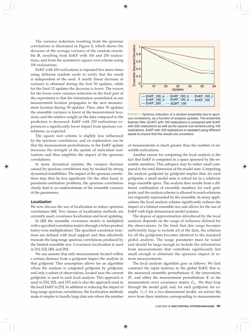
JUNE 2009 « IEEE CONTROL SYSTEMS MAGAZINE 101
The variance reduction resulting from the spurious correlations is illustrated in Figure 8, which shows the decrease of the average variance of the random ensem-ble B , resulting from EnKF with 100 and 250 realiza-tions, and from the symmetric square root scheme using 100 realizations.
EnKF with 100 realizations is repeated five more times using different random seeds to verify that the result is independent of the seed. A nearly linear decrease of variance is obtained during the first 50 updates, while for the final 12 updates the decrease is lower. The reason for the lower error variance reduction in the final part of the experiment is that the information assimilated at one measurement location propagates to the next measure-ment location during 50 updates. Thus, after 50 updates the ensemble variance is lower at the measurement loca-tions, and the relative weight on the data compared to the prediction is decreased. EnKF with 250 realizations ex-periences a significantly lower impact from spurious cor-relations, as expected.
The square root scheme is slightly less influenced by the spurious correlations, and an explanation can be that the measurement perturbations in the EnKF update increases the strength of the update of individual real-izations and thus amplifies the impact of the spurious correlations.
In many dynamical systems, the variance decrease caused by spurious correlations may be masked by strong dynamical instabilities. The impact of the spurious correla-tions may then be less significant. On the other hand, in parameter-estimation problems, the spurious correlations clearly lead to an underestimate of the ensemble variance of the parameters.
LocalizationWe now discuss the use of localization to reduce spurious correlations [48]. Two classes of localization methods are currently used, covariance localization and local updating.
In [48] the ensemble covariance matrix is multiplied with a specified correlation matrix through a Schur product (entry-wise multiplication). The specified correlation func-tions are defined with local support and thus effectively truncate the long-range spurious correlations produced by the limited ensemble size. Covariance localization is used in [11], [12], [49], and [50].
We can assume that only measurements located within a certain distance from a gridpoint impact the analysis in that gridpoint. This assumption allows for an algorithm where the analysis is computed gridpoint by gridpoint, and only a subset of observations, located near the current gridpoint, is used in each local analysis. This approach is used in [51], [52], and [37] and is also the approach used in the local EnKF in [53]. In addition to reducing the impact of long-range spurious correlations, the localization methods make it simpler to handle large data sets where the number
of measurements is much greater than the number of en-semble realizations.
Another reason for computing the local analysis is the fact that EnKF is computed in a space spanned by the en-semble members. This subspace may be rather small com-pared to the total dimension of the model state. Computing the analysis gridpoint by gridpoint implies that, for each gridpoint, a small model state is solved for in a relatively large ensemble space. The analysis then results from a dif-ferent combination of ensemble members for each grid-point, and the analysis scheme is allowed to reach solutions not originally represented by the ensemble. In many appli-cations the local analysis scheme significantly reduces the impact of a limited ensemble size and allows for the use of EnKF with high-dimensional model systems.
The degree of approximation introduced by the local analysis depends on the range of influence defined for the observations. In the limit that this range becomes sufficiently large to include all of the data, the solution for all the gridpoints becomes identical to the standard global analysis. The range parameter must be tuned and should be large enough to include the information from measurements that contribute significantly but small enough to eliminate the spurious impact of re-mote measurements.
The local analysis algorithm goes as follows. We first construct the input matrices to the global EnKF, that is, the measured ensemble perturbations S , the innovations Dr , and either the measurement perturbations E or the measurement error covariance matrix CPP . We then loop through the model grid, and, for each gridpoint, for ex-ample, ( i, j) for a two-dimensional model, we extract the rows from these matrices corresponding to measurements
FIGURE 8 Variance reduction of a random ensemble due to spuri-ous correlations, as a function of analysis updates. The ensemble Kalman fi lter (EnKF) with 100 realizations is compared with EnKF with 250 realizations as well as the square root scheme using 100 realizations. EnKF with 100 realizations is repeated using different seeds to ensure that the results are consistent.
Updates
Ens
embl
e S
tand
ard
Dev
iatio
n
0 10 20 30 40 50 600
0.2
0.4
0.6
0.8
1
EnKF_100_a EnKF_100_b EnKF_100_cEnKF_100_d EnKF_100_e EnKF_100EnKF_250 SQRT_100
102 IEEE CONTROL SYSTEMS MAGAZINE » JUNE 2009
that are used in the current update, and then compute the matrix X(i,j) that defines the update for gridpoint ( i, j) .
The analysis at gridpoint ( i, j) becomes
A(i,j)a 5 A(i,j)X(i,j) (79)
5 A(i,j)X 1 A(i,j) (X(i,j) 2 X ) , (80)
where X is the global solution, while X(i,j) becomes the so-lution for a local analysis corresponding to gridpoint ( i, j) where only the nearest measurements are used in the anal-ysis. Thus, it is possible to compute the global analysis first and then add the corrections from the local analysis if these effects are significant.
The quality of the EnKF analysis is connected to the en-semble size used. We expect that to achieve the same qual-ity of the result, a larger ensemble is needed for the global analysis than the local analysis. In the global analysis, a large ensemble is needed to properly explore the state space and to provide a consistent result that is as good as the local analysis. Note also that the use of a local analysis scheme is likely to introduce nondynamical modes, although the amplitudes of these modes are small if a large enough in-fluence radius is used when selecting measurements. We also refer to the discussions on localization and filtering of long-range correlations by [54].
In adaptive localization methods, the assimilation sys-tem itself is used to determine the localization strategy. Such algorithms are useful since the dynamical covari-ance functions change in space and time, and the spuri-ous correlations depend on the ensemble size. Thus, every assimilation problem and ensemble size requires a separate tuning of the localization parameters.
The hierarchical approach in [55] uses several small en-sembles to explore the need for using localization in the analysis. This approach uses a Monte Carlo method based on splitting the ensemble into several small ensembles to assess the sampling errors and the spurious correlations. This method is a statistically consistent approach to the problem. However, the localization is optimized for a small ensemble and may become suboptimal when used with the full ensemble including all realizations.
An alternative localization method in [56] is based on the online computation of a flow-dependent moderation function that is used to damp long-range and spurious cor-relations. This method is named SENCORP for “smoothed ensemble correlations raised to a power.” The idea is that the moderation functions can be generated from a smoothed covariance function, which, when raised to a power, damps small correlations.
In [57] a local analysis method handles measurements that are integral parameters of the model state. The idea is that the covariance matrix of the predicted measure-ments is computed globally using the full model state, while the updates are computed locally gridpoint by grid-point, and only the measurements that have significant
correlations with the model variables in the local grid-point are assimilated.
Thus, while traditional localization methods are distance based, [55]–[57] discuss adaptive localization methods where the assimilation system determines whether correla-tions are significant or spurious, and whether a particular measurement shall be used in the update of a particular model variable. The further development of adaptive local-ization methods is important for many applications where distance-based methods are less suitable, an example being the use of measurements that are integral functions of the model state as in [57].
Finally, it is not clear how the local analysis scheme is best implemented in EnKS. One approach is to define the local analysis to use only measurements in a certain space-time domain, taking into account the propagation of information in the model together with the time scales of the model. In [58] EnKS is used with a high-dimensional atmospheric circulation model. The impact of spurious cor-relations related to the lag time in a lagged EnKS is studied, and it is pointed out that the lagged implementation facili-tates localization in time.
Infl ationA covariance inflation procedure [59] can be used to coun-teract the variance reduction observed due to the impact of spurious correlations as well as other effects leading to underestimation of the ensemble variance. The impact of ensemble size on noise in distant covariances is examined in [49], while the impact of using an “inflation factor” as discussed in [59] is evaluated. The inflation factor is used to replace the forecast ensemble according to
cj 5 r(cj 2 c ) 1 c, (81)
with r slightly greater than one (typically 1.01). The in-flation procedure is also used in [60], where the EnKF is examined in an application with the Lorenz attractor, and results are compared with those obtained from different versions of the singular evolutive extended Kalman (SEEK) filter and a particle filter. In [60], ensembles with very few members are used, which favors methods like the SEEK where the “ensemble” of empirical orthogonal functions (EOFs) is selected to best represent the model attractor.
Several approaches adaptively estimate an optimal infla-tion parameter. In [61] the covariance inflation is estimated based on the sequence of innovation statistics, while in [62] a method is presented that is based on augmenting the in-flation parameter to the model state where it is updated as a parameter in the EnKF analysis computations. Online es-timation of the inflation parameter is also studied in [63] together with the simultaneous estimation of observation errors. It is found that the estimation of inflation alone does not work appropriately without accurate observation error statistics, and vice versa.
JUNE 2009 « IEEE CONTROL SYSTEMS MAGAZINE 103
Clearly, the inflation parameter becomes a tuning pa-rameter, and optimally it is best estimated adaptively. The need for inflation depends on the use of a local versus glob-al analysis scheme, and the use of a local scheme can to a large extent reduce the need for an additional inflation.
Here we describe an alternative approach for estimating the inflation coefficient. In the spurious correlation example, as presented in Figure 8, an independent ensemble is used to quantify the variance reduction due to spurious correlations. A simple algorithm for correcting the analyzed ensemble perturbations in each analysis step goes as follows.
At each analysis time we generate the additional ensem-ble matrix Bf with random normally distributed numbers, such that the mean in each row is exactly zero, and the vari-ance is exactly equal to one. We thus sample the matrix ran-domly from N(0, 1) . Then, for each row, first subtract any nonzero mean, then compute the standard deviation and scale all entries by it. Then, compute the analysis update according to (77). For each row in Ba, compute the standard deviation. The inflation factor r is then defined as one over the average of the standard deviations from each row in Ba. The accuracy of the estimated inflation factor depends on the number of realizations used as well as the number of rows in B . It is expected that with a low number of realiza-tions additional rows in B might compensate for the sam-pling errors when computing the inflation factor.
This algorithm provides a good first approximation of the inflation factor needed to counteract variance reduc-tion due to long-range spurious correlations resulting from sample noise. The estimated inflation factor depends on the number of realizations used, the number of measurements, and the strength of the update determined by the innova-tion vector and both the predicted and measurement error covariance matrices. A question remains, as to whether the inflation is best applied equally for the whole model state, including at the measurement locations.
CONCLUSIONSThis article provides a fundamental theoretical basis for understanding EnKF and serves as a useful text for future users. Data assimilation and parameter-estimation prob-lems are explained, and the concept of joint parameter and state estimation, which can be solved using ensemble methods, is presented. KF and EKF are briefly discussed before introducing and deriving EnKF. Similarities and differences between KF and EnKF are pointed out. The benefits of using EnKF with high-dimensional and highly nonlinear dynamical models are illustrated by examples. EnKF and EnKS are also derived from Bayes theorem, us-ing a probabilistic approach. The derivation is based on the assumption that measurement errors are independent in time and the model represents a Markov process, which allows for Bayes theorem to be written in a recursive form, where measurements are processed sequentially in time. The practical implementation of the analysis scheme is
discussed, and it is shown that it can be computed efficient-ly in the space spanned by the ensemble realizations. The square root scheme is discussed as an alternative method that avoids the perturbation of measurements. However, the square root scheme has other pitfalls, and it is recom-mended to use the symmetric square root with or with-out a random rotation. The random rotation introduces a stochastic component to the update, and the quality of the scheme may then not improve compared to the original stochastic EnKF scheme with perturbed measurements.
ACKNOWLEDGMENTSI am grateful for many fruitful discussions with Pavel Sakov and Laurent Bertino during the preparation of this article, and I thank Pavel Sakov for providing the data used to illustrate the properties of the different analysis schemes in Figure 7 and for pointing out that the use of an ensemble representation of the measurement error covariance matrix leads to an exact cancellation in the second last line in (27). The extensive feedback provided by the reviewers contrib-uted to significantly improving the quality of the manu-script. I am partly supported by the Norwegian Research Council through the Evita EnKF Project.
AUTHOR INFORMATIONGeir Evensen ([email protected]) received the Ph.D. in applied mathematics from the University of Bergen, Norway, in 1992. He has published more than 40 articles related to data assimilation, including Data Assimilation: The Ensemble Kalman Filter. He currently works on data assimilation and parameter estimation as a research direc-tor at StatoilHydro in Bergen and holds an associate posi-tion at the Nansen Center in Bergen.
REFERENCES[1] G. Evensen, “Sequential data assimilation with a nonlinear quasi-geo-strophic model using Monte Carlo methods to forecast error statistics,” J. Geophys. Res., vol. 99, no. C5, pp. 10143–10162, 1994. [2] R. E. Kalman, “A new approach to linear filter and prediction problems,” J. Basic Eng., vol. 82, pp. 35–45, 1960.[3] R. E. Kalman and R. S. Bucy, “New results of linear filtering and predic-tion theory,” J. Basic Eng., vol. 83, pp. 95–108, 1961.[4] O. Talagrand and P. Courtier, “Variational assimilation of meteorologi-cal observations with the adjoint vorticity equation. I. Theory,” Q. J. R. Me-teorol. Soc., vol. 113, pp. 1311–1328, 1987.[5] E. Kalnay, H. Li, T. Miyoshi, S.-C. Yang, and J. Ballabrera-Poy, “4D-Var or ensemble Kalman filter?,” Tellus A, vol. 59, pp. 758–773, 2007.[6] E. J. Fertig, J. Harlim, and B. R. Hunt, “A comparative study of 4D-Var and a 4D ensemble Kalman filter: Perfect model simulations with Lorenz-96,” Tellus A, vol. 59, pp. 96–101, 2006. [7] G. Evensen, “Using the extended Kalman filter with a multilayer quasi-geostrophic ocean model,” J. Geophys. Res., vol. 97, no. C11, pp. 17905–17924, 1992. [8] G. Evensen, Data Assimilation: The Ensemble Kalman Filter. New York: Springer, 2007. [9] G. Burgers, P. J. van Leeuwen, and G. Evensen, “Analysis scheme in the ensemble Kalman filter,” Mon. Weather Rev., vol. 126, pp. 1719–1724, 1998. [10] J. L. Anderson, “An ensemble adjustment Kalman filter for data assimi-lation,” Mon. Weather Rev., vol. 129, pp. 2884–2903, 2001. [11] J. S. Whitaker and T. M. Hamill, “Ensemble data assimilation without perturbed observations,” Mon. Weather Rev., vol. 130, pp. 1913–1924, 2002.

104 IEEE CONTROL SYSTEMS MAGAZINE » JUNE 2009
[12] C. H. Bishop, B. J. Etherton, and S. J. Majumdar, “Adaptive sampling with the ensemble transform Kalman filter. Part I: Theoretical aspects,” Mon. Weather Rev., vol. 129, pp. 420–436, 2001. [13] M. K. Tippett, J. L. Anderson, C. H. Bishop, T. M. Hamill, and J. S. Whitaker, “Ensemble square-root filters,” Mon. Weather Rev., vol. 131, pp. 1485–1490, 2003. [14] A. Doucet, N. de Freitas, and N. Gordon, Eds. Sequential Monte Carlo Methods in Practice (Statistics for Engineering and Information Science). New York: Springer-Verlag, 2001. [15] C. L. Keppenne and M. Rienecker, “Initial testing of a massively paral-lel ensemble Kalman filter with the Poseidon isopycnal ocean general cir-culation model,” Mon. Weather Rev., vol. 130, pp. 2951–2965, 2002. [16] C. L. Keppenne and M. Rienecker, “Assimilation of temperature into an isopycnal ocean general circulation model using a parallel ensemble Kal-man filter,” J. Mar. Syst., vol. 40-41, pp. 363–380, 2003. [17] C. L. Keppenne, M. Rienecker, N. P. Kurkowski, and D. A. Adamec, “Ensemble Kalman filter assimilation of temperature and altimeter data with bias correction and application to seasonal prediction,” Nonlinear Pro-cess. Geophys., vol. 12, pp. 491–503, 2005. [18] I. Szunyogh, E. J. Kostelich, G. Gyarmati, D. J. Patil, B. R. Hunt, E. Kalnay, E. Ott, and J. A. Yorke, “Assessing a local ensemble Kalman filter: Perfect model experiments with the national centers for environmental prediction global model,” Tellus A, vol. 57, pp. 528–545, 2005. [19] P. L. Houtekamer and H. L. Mitchell, “Ensemble Kalman filtering,” Q. J. R. Meteorol. Soc., vol. 131, pp. 3269–3289, 2005. [20] B. R. Hunt, E. J. Kostelich, and I. Szunyogh, “Efficient data assimila-tion for spatiotemporal chaos: A local ensemble transform Kalman filter,” Physica D, vol. 230, pp. 112–126, 2007. [21] I. Szunyogh, E. J. Kostelich, G. Gyarmati, E. Kalnay, B. R. Hunt, E. Ott, E. Satterfield, and J. A. Yorke, “A local ensemble transform Kalman filter data assimilation system for the NCEP global model,” Tellus A, vol. 60, pp. 113–130, 2008. [22] J. S. Whitaker, T. M. Hamill, X. Wei, Y. Song, and Z. Toth, “Ensemble data assimilation with the NCEP global forecast system,” Mon. Weather Rev., vol. 136, pp. 463–482, 2008. [23] K. Eben, P. Juru, J. Resler, M. Belda, E. Pelikán, B. C. Krger, and J. Ked-er, “An ensemble Kalman filter for short-term forecasting of tropospheric ozone concentrations,” Q. J. R. Meteorol. Soc., vol. 131, pp. 3313–3322, 2005. [24] O. Barrero Mendoza, B. De Moor, and D. S. Bernstein, “Data assimila-tion for magnetohydrodynamics systems,” J. Comput. Appl. Math., vol. 189, no. 1, pp. 242–259, 2006. [25] Y. Zhou, D. McLaughlin, and D. Entekhabi, “An ensemble-based smoother with retrospectively updated weights for highly nonlinear sys-tems,” Mon. Weather Rev., vol. 135, pp. 186–202, 2007. [26] M. Eknes and G. Evensen, “Parameter estimation solving a weak con-straint variational formulation for an Ekman model,” J. Geophys. Res., vol. 102, no. C6, pp. 12479–12491, 1997. [27] J. C. Muccino and A. F. Bennett, “Generalized inversion of the Ko-rteweg-de Vries equation,” Dyn. Atmos. Oceans, vol. 35, pp. 227–263, 2001.[28] A. F. Bennett, Inverse Methods in Physical Oceanography. Cambridge, U.K.: Cambridge Univ. Press, 1992. [29] A. F. Bennett, Inverse Modeling of the Ocean and Atmosphere. Cambridge, U.K.: Cambridge Univ. Press, 2002. [30] G. Evensen, J. Hove, H. C. Meisingset, E. Reiso, K. S. Seim, and Ø. Espe-lid, “Using the EnKF for assisted history matching of a North Sea reservoir model,” Houston, TX, Soc. Petroleum Eng., Inc., SPE 106184, 2007. [31] R. N. Miller, “Perspectives on advanced data assimilation in strongly nonlinear systems,” in Data Assimilation: Tools for Modelling the Ocean in a Global Change Perspective (NATO ASI, vol. I 19), P. P. Brasseur and J. C. J. Nihoul, Eds. Berlin: Springer-Verlag, 1994, pp. 195–216. [32] R. N. Miller, M. Ghil, and F. Gauthiez, “Advanced data assimilation in strongly nonlinear dynamical systems,” J. Atmos. Sci., vol. 51, pp. 1037–1056, 1994. [33] P. Gauthier, P. Courtier, and P. Moll, “Assimilation of simulated wind lidar data with a Kalman filter,” Mon. Weather Rev., vol. 121, pp. 1803–1820, 1993. [34] F. Bouttier, “A dynamical estimation of forecast error covariances in an assimilation system,” Mon. Weather Rev., vol. 122, pp. 2376–2390, 1994. [35] A. H. Jazwinski, Stochastic Processes and Filtering Theory. San Diego, CA: Academic, 1970. [36] R. H. Reichle, D. B. McLaughlin, and D. Entekhabi, “Hydrologic data assimilation with the ensemble Kalman filter,” Mon. Weather Rev., vol. 130, pp. 103–114, 2002.
[37] G. Evensen, “The ensemble Kalman filter: Theoretical formulation and practical implementation,” Ocean Dyn., vol. 53, pp. 343–367, 2003. [38] G. Evensen and P. J. van Leeuwen, “An ensemble Kalman smoother for nonlinear dynamics,” Mon. Weather Rev., vol. 128, pp. 1852–1867, 2000. [39] P. J. van Leeuwen and G. Evensen, “Data assimilation and inverse methods in terms of a probabilistic formulation,” Mon. Weather Rev., vol. 124, pp. 2898–2913, 1996.[40] G. Evensen, “Advanced data assimilation for strongly nonlinear dy-namics,” Mon. Weather Rev., vol. 125, pp. 1342–1354, 1997.[41] E. N. Lorenz, “Deterministic nonperiodic flow,” J. Atmos. Sci., vol. 20, pp. 130–141, 1963. [42] G. Evensen, “Sampling strategies and square root analysis schemes for the EnKF,” Ocean Dyn., vol. 54, pp. 539–560, 2004. [43] O. Leeuwenburgh, “Assimilation of along-track altimeter data in the Tropical Pacific region of a global OGCM ensemble,” Q. J. R. Meteorol. Soc., vol. 131, pp. 2455–2472, 2005. [44] P. Sakov and P. R. Oke, “Implications of the form of the ensemble trans-form in the ensemble square root filters,” Mon. Weather Rev., vol. 136, no. 3, pp. 1042–1053, 2008. [45] X. Wang, C. H. Bishop, and S. J. Julier, “Which is better, an ensemble of positive-negative pairs or a centered spherical simplex ensemble,” Mon. Weather Rev., vol. 132, pp. 1590–1605, 2004. [46] O. Leeuwenburgh, G. Evensen, and L. Bertino, “The impact of ensem-ble filter definition on the assimilation of temperature profiles in the Tropi-cal Pacific,” Q. J. R. Meteorol. Soc., vol. 131, pp. 3291–3300, 2005. [47] D. M Livings, S. L. Dance, and N. K. Nichols, “Unbiased ensemble square root filters,” Physica D, vol. 237, pp. 1021–1028, 2008.[48] P. L. Houtekamer and H. L. Mitchell, “A sequential ensemble Kalman filter for atmospheric data assimilation,” Mon. Weather Rev., vol. 129, pp. 123–137, 2001.[49] T. M. Hamill, J. S. Whitaker, and C. Snyder, “Distance-dependent fil-tering of background error covariance estimates in an ensemble Kalman filter,” Mon. Weather Rev., vol. 129, pp. 2776–2790, 2001. [50] J. L. Anderson, “A local least squares framework for ensemble filter-ing,” Mon. Weather Rev., vol. 131, pp. 634–642, 2003. [51] V. E. Haugen and G. Evensen, “Assimilation of SLA and SST data into an OGCM for the Indian ocean,” Ocean Dyn., vol. 52, pp. 133–151, 2002. [52] K. Brusdal, J. M. Brankart, G. Halberstadt, G. Evensen, P. Brasseur, P. J. van Leeuwen, E. Dombrowsky, and J. Verron, “An evaluation of ensemble based assimilation methods with a layered OGCM,” J. Mar. Syst., vol. 40-41, pp. 253–289, 2003. [53] E. Ott, B. Hunt, I. Szunyogh, A. V. Zimin, E. Kostelich, M. Corazza, E. Kalnay, D. J. Patil, and J. A. Yorke, “A local ensemble Kalman filter for atmo-spheric data assimilation,” Tellus A, vol. 56, pp. 415–428, 2004. [54] H. L. Mitchell, P. L. Houtekamer, and G. Pellerin, “Ensemble size, and model-error representation in an ensemble Kalman filter,” Mon. Weather Rev., vol. 130, pp. 2791–2808, 2002. [55] J. L. Anderson, “Exploring the need for localization in the ensemble data assimilation using a hierarchical ensemble filter,” Physica D, vol. 230, pp. 99–111, 2007. [56] C. H. Bishop and D. Hodyss, “Flow-adaptive moderation of spurious ensemble correlations and its use in ensemble-based data assimilation,” Q. J. R. Meteorol. Soc., vol. 133, pp. 2029–2044, 2007. [57] E. J. Fertig, B. R. Hunt, E. Ott, and I. Szunyogh, “Assimilating non-local observations with a local ensemble Kalman filter,” Tellus A, vol. 59, pp. 719–730, 2007. [58] S. P. Khare, J. L. Anderson, T. J. Hoar, and D. Nychka, “An investigation into the application of an ensemble Kalman smoother to high-dimensional geophysical systems,” Tellus A, vol. 60, pp. 97–112, 2008. [59] J. L. Anderson and S. L. Anderson, “A Monte Carlo implementation of the nonlinear filtering problem to produce ensemble assimilations and forecasts,” Mon. Weather Rev., vol. 127, pp. 2741–2758, 1999. [60] D. T. Pham, “Stochastic methods for sequential data assimilation in strongly nonlinear systems,” Mon. Weather Rev., vol. 129, pp. 1194–1207, 2001. [61] X. Wang and C. H. Bishop, “A comparison of breeding and ensemble transform Kalman filter ensemble forecast schemes,” J. Atmos. Sci., vol. 60, pp. 1140–1158, 2003. [62] J. L. Anderson, “An adaptive covariance inflation error correction algo-rithm for ensemble filters,” Tellus A, vol. 59, pp. 210–224, 2007. [63] H. Li, E. Kalnay, and T. Miyoshi, “Simultaneous estimation of covari-ance inflation and observation errors within ensemble Kalman filter,” Q. J. R. Meteorol. Soc., vol. 135, no. 639, pp. 523–533, 2009.