dual-state kalman filter forecasting and control theory
TRANSCRIPT

DUAL-STATE KALMAN FILTER FORECASTING AND CONTROL THEORY
APPLICATIONS FOR PROACTIVE RAMP METERING
by
Brian Richard Portugais
A thesis
submitted in partial fulfillment
of the requirements for the degree of
Master of Science in Civil Engineering
Boise State University
August 2014

© 2014
Brian Richard Portugais
ALL RIGHTS RESERVED

BOISE STATE UNIVERSITY GRADUATE COLLEGE
DEFENSE COMMITTEE AND FINAL READING APPROVALS
of the thesis submitted by
Brian Richard Portugais
Thesis Title: Dual-State Kalman Filter Forecasting and Control Theory Applications for Proactive Ramp Metering
Date of Final Oral Examination: 20 June 2014 The following individuals read and discussed the thesis submitted by student Brian Richard Portugais, and they evaluated his presentation and response to questions during the final oral examination. They found that the student passed the final oral examination. Mandar Khanal, Ph.D. Chair, Supervisory Committee Jaechoul Lee, Ph.D. Member, Supervisory Committee Yang Lu, Ph.D. Member, Supervisory Committee The final reading approval of the thesis was granted by Mandar Khanal, Ph.D., Chair of the Supervisory Committee. The thesis was approved for the Graduate College by John R. Pelton, Ph.D., Dean of the Graduate College.

iv
DEDICATION
“Forgetting what is behind and straining toward what is ahead, I press on toward the
goal…” (Philippians 3:13-14)
The work herein is a true labor of love, but the “ah-ha” moments did not arrive
without toil and occasional bouts of weariness. With its completion, I hope any door I’ve
been given the opportunity to walk through is wider for any who may follow.
Throughout this pursuit, many people have extended encouragement and support that has
contributed to this thesis in ways that are immeasurable. I would personally like to thank
my family and friends, especially the Gould family, whose kindness has altered the
course of many lives, the Robinson family, and Scott Reynolds, whose friendship is
unassailable.
I am especially grateful to my mother for her unconditional belief in me. Lastly, I
would like to thank my best friend and wife, Tara, whose love, support, and
encouragement know no bounds. I dedicate this thesis to her, for proving that sometimes
God likes to show off.

v
ACKNOWLEDGEMENTS
I am indebted for the countless opportunities I’ve been given at Boise State
University and the Department of Civil Engineering. Their funding made this thesis
possible. Special thanks are extended to the Idaho Transportation Department for
funding of the data collection with particular recognition to Kevin Sablan.
Special acknowledgment is given to Dr. Mandar Khanal for his patience,
encouragement, and guidance throughout this study. The time and knowledge he has
poured into me have been immense and I am forever grateful. Our conversations were
never limited by our research, and I thank him for his mentorship. Many thanks are
extended to my committee members, Dr. Jaechoul Lee and Dr. Yang Lu.
I would also like to thank Lauren Oe, for her vision, of the Office of the Dean of
Students.

vi
AUTOBIOGRAPHICAL SKETCH OF AUTHOR
Brian Portugais received his B.S. in Civil Engineering from Boise State
University in 2012. As an undergraduate, he worked as a research assistant modeling the
flow of groundwater. His senior design project, “Ten Mile Road Interchange and Bridge
Design” won “Best Poster” from the Department of Civil Engineering and shifted his
focus to transportation. As a Graduate Research Assistant, Portugais has published two
peer-reviewed journal articles with his advisor, Dr. Mandar Khanal.

vii
ABSTRACT
Deterioration of freeway traffic flow condition due to bottlenecks can be
ameliorated with ramp metering. A challenge in ramp metering is that it is not possible
to process data in real-time and use the output in a control algorithm. This is due to the
fact that by the time processing is completed and a control measure applied, the traffic
state will have changed. A solution to this problem is to forecast the traffic state and
implement a control measure based on the forecast.
A dual-state Kalman filter was used to forecast traffic data at two locations on a
freeway (I-84). A Kalman filter is an optimal recursive data processing algorithm;
predictions are based on only the previous time-step’s prediction and all previous data do
not need to be stored and reprocessed with new measurements. A coordinated feedback
ramp metering control logic was implemented. The closed-loop system seeks to control
the traffic density on the mainline while minimizing on-ramp queues through weighting
functions.
The integration of the Kalman filter with the ramp meter control logic
accomplishes the ramp meter algorithmic scheme, which is proactive to changes in
freeway conditions by controlling a forecasted state. In this closed-loop framework, real-
time forecasts are produced with a continuously updated prediction that minimizes errors
and recursively improves with each successive measurement. MATLAB was used to

viii
model the closed-loop control system as well as modify the input output constraints to
evaluate and tune controller performance.

ix
TABLE OF CONTENTS
DEDICATION ......................................................................................................................... iv
ACKNOWLEDGEMENTS ...................................................................................................... v
AUTOBIOGRAPHICAL SKETCH OF AUTHOR ................................................................ vi
ABSTRACT ............................................................................................................................ vii
LIST OF TABLES ................................................................................................................. xiii
LIST OF FIGURES ............................................................................................................... xiv
LIST OF NOMENCLATURE .............................................................................................. xvii
CHAPTER 1: Introduction ....................................................................................................... 1
1.1 Background ............................................................................................................. 1
1.2 Problem Statement .................................................................................................. 3
1.3 Thesis Summary...................................................................................................... 4
CHAPTER 2: Literature Review .............................................................................................. 6
2.1 Ramp Metering ....................................................................................................... 6
2.1.1 Benefits and Impacts ................................................................................ 7
2.1.2 Local Ramp Metering .............................................................................. 9
2.1.2.1 Demand-Capacity Strategy ....................................................... 9
2.1.2.2 Occupancy Control ................................................................. 10
2.1.2.3 ALINEA .................................................................................. 11
2.1.3 Coordinated Ramp Metering.................................................................. 14

x
2.1.3.1 Cooperative Algorithms .......................................................... 14
2.1.3.2 Competitive Algorithms.......................................................... 14
2.1.3.3 Integral Algorithms ................................................................. 15
2.1.4 Queue Management ............................................................................... 17
2.2 Kalman Filtering ................................................................................................... 17
2.3 Stochastic Capacity ............................................................................................... 18
CHAPTER 3: Methodology .................................................................................................... 21
3.1 State-Space Framework ........................................................................................ 21
3.1.1 Dynamic Linear Model .......................................................................... 22
3.2 Kalman Filtering ................................................................................................... 22
3.3 Traffic Flow Theory .............................................................................................. 25
3.3.1 Traffic Bottlenecks and Shockwave Theory .......................................... 28
3.4 Feedback Control Theory ..................................................................................... 30
3.4.1 Proportional Response ............................................................... 31
3.4.2 Integral Response ....................................................................... 32
3.4.3 Derivative Response .................................................................. 33
3.5 Feedback Coordinated Ramp Metering Control Design ....................................... 33
3.5.1 Control Objective ................................................................................... 35
3.5.1.1 Overall Control Law ............................................................... 38
3.5.2 Decoupled D-MIXCROS ....................................................................... 40
3.5.3 Coupled C-MIXCROS ........................................................................... 42
3.6 Field Site and Data Collection .............................................................................. 43
3.6.1 Site Selection ......................................................................................... 43

xi
3.6.2 Data Collection and Description ............................................................ 45
CHAPTER 4: DLM & Kalman Filter Simulation .................................................................. 48
4.1 R Language and Environment .............................................................................. 48
4.2 R Model Specification, Parameter Estimation: Traffic Volume ........................... 49
4.2.1 Maximum Likelihood Estimation .......................................................... 50
4.2.2 Seasonal Models .................................................................................... 52
4.2.3 KF Results: Traffic Volume RW Model ................................................ 55
4.2.4 KF Results: Traffic Volume RW with Seasonal Component Model ..... 58
4.2.5 KF Results: Traffic Volume RW with Fourier-Form Model ................. 60
4.3 R Model Specification, Parameter Estimation: Traffic Speeds ............................ 62
4.3.1 Maximum Likelihood Estimation .......................................................... 62
4.3.2 Seasonal Models .................................................................................... 63
4.3.3 KF Results: Traffic Speeds RW Model ................................................. 65
4.3.4 KF Results: Traffic Speeds RW with Seasonal Component Model ...... 67
4.3.5 KF Results: Traffic Speeds RW with Fourier-Form Model .................. 69
4.4 Results Analysis .................................................................................................... 70
CHAPTER 5: Prediction & Control Integration ..................................................................... 73
5.1 Integration Methodology ...................................................................................... 74
5.2 MATLAB Programming: Kalman Filter & Extended Kalman Filter ................... 76
5.2.1 Kalman Filter ......................................................................................... 76
5.2.2 Extended Kalman Filter ......................................................................... 78
5.3 MATLAB Programming: Ramp Meter Control Files .......................................... 83
5.4 Simulation: KF & Decoupled Feedback Control Integration ............................... 85

xii
5.4.1 Decoupled Control Testing .................................................................... 90
5.5 Simulation: KF & Coupled Feedback Control Integration ................................... 92
5.6 Simulation: Extended KF Results ......................................................................... 97
5.7 Results Analysis .................................................................................................. 100
CHAPTER 6: Conclusions ................................................................................................... 102
6.1 Summary of Work............................................................................................... 103
6.2 Implementation ................................................................................................... 104
6.3 Recommendations for Future Work.................................................................... 105
REFERENCES ..................................................................................................................... 106
APPENDIX A: MATLAB Ramp Meter Control M-Files .................................................... 113
rampmeter_runfile.m ................................................................................................ 113
ramp1_meter.m ......................................................................................................... 120
ramp2_meter.m ......................................................................................................... 121
kalman_pred.m.......................................................................................................... 122
APPENDIX B: Extended Kalman Filter MATLAB M-File ................................................ 123
EKF.m ....................................................................................................................... 123
APPENDIX C: R Code: Traffic Volume DLMs & KF ........................................................ 127
Section_4.2.R ............................................................................................................ 127
APPENDIX D: R Code: Traffic Speeds DLMs & KF ......................................................... 131
Section_4.3.R ............................................................................................................ 131
APPENDIX E: Plots ............................................................................................................. 135

xiii
LIST OF TABLES
Table 4.1. DLM Volume Models Performance statistics ........................................... 71
Table 4.2. DLM Speed Models Performance statistics .............................................. 71
Table 5.1. Known Parameters for Ramp Meter Run-File .......................................... 84
Table 5.2. Initial Regulator Gains for Feedback Ramp Meter Control...................... 84
Table 5.3. Weighting Factors for Mainline and Ramp Sections ................................ 84
Table 5.3. KF & EKF Root Mean Square Error of Prediction ................................. 100
Table 5.4. Decoupled & Coupled Ramp Delays ...................................................... 101
Table 6.1. FHWA Recommended Cycle Length, Metering Rates, & Associated Capacity .................................................................................................. 104

xiv
LIST OF FIGURES
Figure 1. Fundamental Diagram with Left Side Approximated by a Straight Line . 11
Figure 2. HCM Three-Regime Speed-Flow Relationship ........................................ 26
Figure 3. HCM Flow-Density Relationship ............................................................. 27
Figure 4. Graphical Representation of Shockwave Speed ....................................... 28
Figure 5. Components of the Elementary Feedback Control System ...................... 30
Figure 6. Proportional-Integral-Derivative Control Structure .................................. 33
Figure 7. Discretized Freeway with Meter and Traffic Sensors Located ................. 34
Figure 8. Feedback Control System ......................................................................... 40
Figure 9. The Eagle Road Interchange with Ramps 1 & 2 Shown .......................... 44
Figure 10. Approximate EB locations of Wavetronix Radar Detectors ..................... 45
Figure 11. Approximate WB locations of Wavetronix Radar Detectors ................... 46
Figure 12. Time-Series Plots for Traffic Speeds, Flows, and Density, EB Site 6 ...... 47
Figure 13. Kalman Filter Applied to Traffic Volume Random Walk with Noise Model ........................................................................................................ 56
Figure 14. Kalman Filter Applied to Traffic Volume Random Walk with 12-Period Seasonal Component Model ..................................................................... 59
Figure 15. Kalman Filter Applied to Traffic Volume Random Walk with Fourier-form Seasonal Component Model ............................................................ 61
Figure 16. Kalman Filter Applied to Traffic Speed Random Walk with Noise Model................................................................................................................... 66
Figure 17. Kalman Filter Applied to Traffic Speed Random Walk with Seasonal Component Model .................................................................................... 68

xv
Figure 18. Kalman Filter Applied to Traffic Speeds Random Walk with Fourier-form Seasonal Component Model Five-Minute Frequency Data ...................... 70
Figure 19. Kalman Filter and Control System Block Diagram .................................. 74
Figure 20. Proportional-Derivative Controller Action ............................................... 75
Figure 21. Linearized Freeway System with Radar Sensor’s Locations .................... 76
Figure 22. Kalman Filter Section 1 Density Predictions TI 0–500 ............................ 85
Figure 23. Kalman Filter Section 1 Density Prediction TI 500–1000........................ 86
Figure 24. Kalman Filter Section 2 Density Prediction TI 1000–1500...................... 86
Figure 25. Kalman Filter Section 2 Density Prediction TI 1500–2000...................... 87
Figure 26. Decoupled Controls: Ramp Demand, Metered Flow, & Queue Length TI 0–1000....................................................................................................... 87
Figure 27. Decoupled Controls: Ramp Demand, Metered Flow, & Queue Length TI1 1000–2000................................................................................................. 88
Figure 28. Kalman Filter Section 1 & 2 Residuals..................................................... 89
Figure 29. Decoupled Results TI 0–1000 for the Shifted Ramp 2 Demands ............. 90
Figure 30. Decoupled Results TI 1000–2000 for the Shifted Ramp 2 Demands ....... 91
Figure 31. Coupled Controls: Ramp Demand, Metered Ramp Flow, & Queue Length TI 0–1000 .................................................................................................. 92
Figure 32. Coupled Controls: Ramp Demands, Metered Ramp Flow, & Queue Length TI 1000–2000 ............................................................................... 93
Figure 33. Coupled Controls: Adjusted Ramp 2 and Gain Parameters TI 0–1000 .... 94
Figure 34. Coupled Controls: Adjusted Ramp 2 and Gain Parameters TI 1000–2000................................................................................................................... 94
Figure 35. Coupled Controls: Adjusted Gain Parameters TI 0–1000 ........................ 95
Figure 36. Coupled Controls: Adjusted Gain Parameters TI 1000–2000 .................. 96
Figure 37. Extended Kalman Filter Prediction Section 1 Density TI 0–1000 ........... 97

xvi
Figure 38. Extended Kalman Filter Prediction Section 1 Density TI 1000–2000 ..... 98
Figure 39. Extended Kalman Filter Prediction Section 2 Density TI 0–1000 ........... 98
Figure 40. Extended Kalman Filter Prediction Section 2 Density TI 1000–2000 ..... 99
Figure 41. Extended Kalman Filter Prediction Residuals Sections 1 & 2 ................. 99
Figure 42. Section 1 Speed-Flow Diagram Displaying Critical Density (rhoc1) ..... 135
Figure 43. Section 2 Speed-Flow Diagram Displaying Critical Density (rhoc2) ..... 136

xvii
LIST OF NOMENCLATURE
Bold variables indicate vector notation
xk State vector
yk Observation vector
Gk Known state matrix
Fk Design matrix of known values of independent variables
wk State process noise assumed to be Gaussian white noise with wk ~ Ɲ(0,Qk)
vk Observation noise assumed to be Gaussian white noise with vk ~ Ɲ(0,Rk)
Kk Kalman filter gain
0x̂ Initial state estimate
0P Initial error covariance estimate
| 1ˆ k k−x State estimate a priori
| 1ˆ
k k−P Error covariance estimate a priori
ky Measurement innovation
|ˆ k kx State estimate a posteriori
|ˆ
k kP Error covariance estimate a posteriori

xviii
1vf Free flow speed of section 1
2vf Free flow speed of section 2
1rhom Jam density of section 1
2rhom Jam density of section 2
1rhoc Critical density of section 1
2rhoc Critical density of section 2
1x∆ Section 1 length
2x∆ Section 2 length
1ρ Section 1 density
2ρ Section 2 density
1r Ramp 1 demand
2r Ramp 2 demand
1u Ramp 1 metered flow
2u Ramp 2 metered flow
1l Ramp 1 queue length
2l Ramp 2 queue length

1
CHAPTER 1: INTRODUCTION
Traffic congestion is often an adverse effect of population increase and economic
expansion. As the Treasure Valley experiences rapid growth, congestion management
will be vital as there is an increase in demand for highway travel and vehicle miles
traveled. An increase in capacity can result in congestion levels that quickly become
similar to those prior to adding the additional capacity and it is unlikely new construction
will ever catch up due to funding and land use limitations. Since new construction is
often the last resort to improve the operations of a freeway, strategies that are more cost-
effective and utilize existing infrastructure or require minimal expansion are needed to
alleviate congestion in the region.
1.1 Background
Interstate-84 (I-84) and Interstate-184 (the Connector), a freeway linking
downtown Boise with I-84, are the backbones of the Treasure (Boise) Valley’s
transportation system. I-84 and I-184 are the primary connections between the region’s
major employment, activity, and retail centers. Current weekday traffic volumes on I-84
range from 20,000 north of Canyon County to 120,000 between the Eagle Road and Wye
Interchanges in Ada County. By 2035, it is forecast that the travel demands on this
corridor will double (COMPASS, 2013).
The 2010 census reported the population of Boise and the metropolitan area were
205,671 and 616,561, respectively (US Census, 2012). This is an increase in the

2
metropolitan area by almost 138,000 since 2002 (Idaho Department of Labor, 2013). The
metropolitan area, consisting of Ada and Canyon Counties, is home to about 600,000
people and The Community Planning Association of Southwest Idaho (COMPASS)
forecasts by 2040 Ada and Canyon Counties will have combined a population of
1,022,000 and 462,000 jobs (COMPASS, 2014). The existing delay on the average
weekday is 27,670 hours (COMPASS, 2014).
In the U.S., traffic congestion cost drivers more than $ 100 billion in 2011
(Schrank, Eisele, & Lomax, 2012). Nonrecurring congestion predominantly results from
incidents (accidents or breakdowns), work zones, and weather. Recurring congestion
most often occurs routinely during peak hours and is simply the result of traffic demand
exceeding freeway capacity usually at a bottleneck. A freeway bottleneck is a critical
point on the road characterized by freely flowing traffic downstream with queues
upstream. This can occur wherever there is a constriction of capacity or demand exceeds
capacity. Hidden bottlenecks exist at locations where the demand exceeds the capacity,
but the demand cannot reach the hidden bottleneck location because of the presence of
upstream or downstream primary bottlenecks. A micro-bottleneck is identified by
perturbations from slow-and-go wave oscillations and a downstream critical bottleneck.
Geometric features that contribute to the occurrence of freeway bottlenecks include:
• On-ramp sections with no auxiliary lane additions, or with short
acceleration lanes
• Weaving sections, particularly out of dropped lanes
• Lane drops on basic segments, or following an off-ramp
• Long upgrades, particularly in the presence of heavy vehicles

3
• Narrowing lane conditions
• Lateral obstructions which reduce free flow speed (FFS), particularly on
bridge sections
I-84 experiences recurring and nonrecurring congestion resulting from bottleneck
formations, especially between Eagle Road and Meridian Road interchanges. By 2040,
the average weekday delay will increase by a forecasted 1500 percent to approximately
440,980 hours (COMPASS, 2014). Utilizing technology and innovative solutions are
crucial to accommodate the forecasted growth and manage its certain congestion. One
such solution is ramp metering, which was reported to have saved $1.8 billion in
congestion costs from 1982 to 2002 (Schrank & Lomax, 2004).
1.2 Problem Statement
Currently, ramp metering is not used in Idaho. In this thesis study, we investigate
new ramp metering to alleviate congestion. The methodology combines the use of
Kalman filters for short-term forecasting of traffic variables and the use of feedback
control theory to develop the ramp metering scheme. The need to forecast traffic
variables with an adaptive tuner arose from a challenge in processing real-time traffic
data. Many ramp metering schemes attempt to maximize throughput by metering to a
predetermined optimal occupancy or maximum capacity level. This suffers from the fact
that capacity is known to not be a fixed value and the optimal measure of it may change
under a wide range of conditions. The method proposed in this study is a stochastic
modeling approach that is adaptive to conditions (e.g., driver behaviors, adverse weather,
incidents, and etc.) and is applied in an on-line manner, yielding real-time forecasts.

4
The Eagle interchange currently contributes the most vehicles to I-84 and is
within two miles of the Meridian Road interchange. The Eagle Road East Bound (EB)
loop on-ramp enters vehicles on the mainline 2,400 feet upstream of the merge of the
Eagle Road EB on-ramp. Ramp metering at the EB on-ramp has been shown through
simulation to improve flow entering the mainline, allowing throughput speeds to be
maintained, eliminating potential shockwave effects due to the on-ramps close proximity
of one another. With the recent construction of the new interchange at Ten Mile Road
and the planned construction of the Meridian Road interchange, system-wide
improvements in travel time and reduction in delays could result with ramp meters at
these locations.
These areas highlight the significance for a ramp metering system that is locally
adaptive to the on-ramp conditions and dynamically coordinated between the
interchanges, to effectively manage the overall flow through the corridor. However, few
reliable automatic control strategies exist due to the complexity of the traffic flow
phenomenon (Adeli & Karim, 2005). Though a number of coordinated traffic-responsive
strategies have been proposed, few have been implemented due to the computational time
required for the alorithms (Gokasar, Ozbay, & Kachroo, 2013).
1.3 Thesis Summary
Based on these relationships, a predictive feedback on-ramp metering control
strategy that is proactive to the onset of congestion breakdown was developed. It uses a
Kalman filter, a recursive forecasting algorithm, to predict traffic density and estimate
on-ramp queue lengths. The adaptive control scheme works by controlling the traffic
density on the mainline while considering on-ramp queues through weighting functions.

5
The design of the overall system was separated into three stages containing two major
research components. In the first component, the design of dynamic linear models
(DLM) and Kalman filters, used for prediction of the state of traffic, was performed.
Next was the design of the metering control logic algorithm. Lastly, the two components
were combined into a single integrated algorithmic program.
The remainder of the thesis is organized as follows. A literature review is
presented in Chapter 2 of ramp metering, Kalman filtering, and stochastic capacity.
Chapter 3 contains the methodological framework for state-space models, Kalman
filtering, a review of traffic flow theory and feedback control theory, and the
implemented ramp metering control design. Chapter 4 presents the modeling efforts for
the DLM and Kalman filters in R (R Core Team, 2013), a programming language and
environment for statistical computing. Chapter 5 describes the numerical programming
of the control logic and the amalgamation of the prediction and control algorithms in in
MATLAB (MATLAB, 2013), a high-level language for numerical computation and
programming. Chapter 6 is the concluding chapter which, contains a summary of the
work performed and recommendations for future work.

6
CHAPTER 2: LITERATURE REVIEW
A literature review was conducted on existing ramp metering systems and the
control algorithms they employ, Kalman filtering uses in transportation applications, and
stochastic capacity. Besides that, properties that have to be taken into account when
developing a proactive control strategy will be provided.
2.1 Ramp Metering
To combat the onset of breakdown, the most widely adopted freeway control is
ramp metering. Ramp meters are traffic signals at the entrances of freeways that regulate
the flow of vehicles onto the freeway. By regulating the amount and timing of vehicles,
ramp meters break up platoons (i.e., groups) and reduce freeway demand. When a
vehicle is given a green light, it is allowed to smoothly enter the flow of freeway traffic
by theoretically taking advantage of existing gaps in the mainline traffic (Arnold, 1998).
The primary objective of ramp metering systems is to reduce freeway congestion;
however, secondary objectives may be identified and accomplished with ramp metering
such as the reduction of freeway crashes. The Federal Highway Administration’s
(FHWA) Ramp Management and Control Handbook advises practitioners consider the
following seven aspects before determining a ramp metering plan (FHWA, 2006):
1. Metering strategy – A strategy should reflect the goals and objectives of
the system but in general seeks to improve conditions on the freeway,
while minimizing queuing and delay.

7
2. Geographic extent – The extent that metering occurs, i.e. at a single ramp
that’s isolated or over multiple ramps and will they be linked.
3. Metering approaches – Pre-timed or adaptive.
4. Metering Algorithms – Programming logic to determine metering rate.
5. Queue Management – How ramp queues will be maintained to an
acceptable length and what is acceptable.
6. Flow Control – The manner and rate by which vehicles are allowed to
enter a freeway ramp meter.
7. Signing – Appropriate signing needs to be implemented along the ramp as
well as on nearby arterials to alert motorists to the presence and operation
of ramp meters and to the specific driving instructions they need to
perform when approaching a ramp.
2.1.1 Benefits and Impacts
There are more than 2,200 ramp meters in 29 metropolitan areas in the U.S.
controlled by agencies with varying strategies and objectives for their use (FHWA,
2006). Because of this, benefits and impacts of metering is measured by the
implementing agency or practitioners “metering philosophy” and may not be assessed
similarly by the public.
Generally, the reported benefits of ramp meters include:
• Improved system operation.
o Increased vehicle throughput.

8
o Increased vehicle speeds.
o Improved use of existing capacity.
• Improved safety.
o Reduction in number of crashes and crash rate in merge zones.
o Reduction in number of crashes and crash rate on the freeway
upstream of the ramp/freeway merge zone.
• Reduced environmental effects.
o Reduced vehicle emissions.
o Reduced fuel consumption.
• Promotion of multi-modal operation.
The main disadvantage to ramp metering is that it can create long queues and
delays on the on-ramps. Although metering can shift traffic to portions of the network
where capacity is underutilized, the potential to inadvertently shift congestion to the
arterial streets is possible. In a study aimed to measure the equity and efficiency of ramp
meters, Levinson, Zhang, Das, and Sheikh, (2004) found the most efficient ramp control
algorithm was also the least equitable one. The public’s opposition to ramp metering has
been linked to the equity issues associated with ramp metering policy (Yin, Liu, &
Benouar, 2004).
Overall, there are two broad types of ramp metering control systems: local and
coordinated. Local ramp metering consists of a section of freeway with one on-ramp in
which the controller responds only to measurements in the vicinity of the ramp.
Coordinated ramp metering consists of the application of metering at a series of on-ramps
and may use available traffic measurements from greater portions of the freeway

9
(Smaragdis, Papageorgiou, & Kosmatopoulos, 2004). Within those systems, two
methods of controlling ramp meters are pre-timed (also referred to as time-of-day or
fixed-time) and traffic-responsive (FHWA, 2006).
Pre-timed metering is the simplest and cheapest form of ramp metering. Metering
rates are determined from off-line, historical demands. In general, time-of-day’s
metering rate is independent of the existing traffic conditions. Traffic-responsive
metering rates are determined or selected based on prevailing traffic conditions measured
in real-time. Most modern ramp metering systems are traffic-responsive.
2.1.2 Local Ramp Metering
Local ramp metering considers an isolated section of the network that consists of
a freeway segment with a single on-ramp and a controller that responds only to changes
in the local conditions (Papageorgiou & Kotsialos, 2002; Kachroo & Ozbay, 2003;
Smaragdis et al., 2004).
2.1.2.1 Demand-Capacity Strategy
Popular in North America, the local demand-capacity (DC) strategy calculates
metering rates (Masher et al., 1975):
min
( 1), if ( 1)( )
, elsecap in in crk oq q k o
r kr
− − ≤=
−
(2.1)
where k=1,2,… is the discrete time index; r(k) is the ramp flow (veh/hr) to be
implemented during the new period k; qcap is the freeway capacity downstream of the
ramp; qin (k-1) is the last measured upstream freeway flow measurement, upstream of the
ramp; oin (k–1) is the last measured upstream freeway percent occupancy; ocr is the

10
critical occupancy; and rmin is a prespecified minimum ramp flow rate (Papageorgiou &
Kotsialos, 2002). This strategy aims to add to the upstream flow qin (k-1) the amount of
ramp flow r(k) necessary to reach the downstream capacity qcap (Smaragdis &
Papageorgiou, 2003). If the occupancy out oout becomes overcritical, the ramp flow is
reduced to rmin until traffic has dissolved. The rmin is a parameter that would be
determined by the agency controlling the system and is typically a function of storage
capacity and vehicle arrival rate.
2.1.2.2 Occupancy Control
The occupancy control (OCC) strategy uses the same philosophy as the DC
strategy, but uses occupancy based measurements for qin. If the left-hand side of the
fundamental diagram (Figure 1) is approximated by a straight line, qin is:
f outin
v oq
g= (2.2)
where vf is the free speed of the freeway and g is the g-factor (Smaragdis &
Papageorgiou, 2003).

11
Figure 1. Fundamental Diagram with Left Side Approximated by a Straight Line Substituting (2.2) into (2.1) gives:
( ) ( 1)fcap out
vr k o k
gq= − × − (2.3)
Both DC and OCC strategies are considered feed forward, or open-loop. In open-
loop systems, the system output is not used as input in the next iteration. This type of
feed forward controller is blind to the control outcome. Conversely, in feedback control,
or closed-loop control, the control input is based on the system output. In a closed-loop
control system, output is fed back recursively so the control variable is a function of the
output of a system (Kachroo & Ozbay, 2003).
2.1.2.3 ALINEA
The most widely used closed-loop local ramp metering algorithm is called
Asservissement LINéaire d’Entrée Autoroutière (ALINEA) (Papageorgiou, Hadj-Salem,
& Blosseville, 1991). ALINEA works by attempting to maximize throughput by
Flow
Rat
e (v
eh/h
r)
Occupancy (percent)
Crit
ical
Occ
upan
cy, O
cr
qout qcap
Oout

12
maintaining a desired occupancy, measured downstream of the ramp. ALINEA
calculates metering rates by:
( ) ( 1) [ ( )]R des outr k r k K o o k= − + − (2.4)
where r(k) is the metering rate at time step k; Kr > 0 is a regulator parameter (veh/hr); odes
is a set (desired) vale for the downstream occupancy. ALINEA is a feedback control
algorithm because it uses the previous time step (k-1) metering rate in the next iteration
r(k) and in control theory is known as an integral feedback regulator (Papageorgiou,
Blosseville, & Haj-Salem, 1990b). The ramp metering rate needs to be converted into a
cycle time with a green-phase and red-phase; typical to standard traffic signals (but
without a yellow phase). For ALINEA, the green-phase duration is determined by:
min max( ) ( 1) [ ( )],R des outsat
Cg k g k K o o k g g gr
= − + − ≤ ≤ (2.5)
where g(k) is the green-phase duration at time interval k (seconds); g(k-1) is the green-
phase duration at previous time interval k-1 (seconds); C is the cycle duration (red-phase
+ green-phase) (seconds); rsat is the ramp saturation flow (capacity flow) (veh/hr); gmin is
the minimum green-phase duration (seconds); gmax is the maximum green-phase duration
(seconds) (Papageorgiou, Hadj-Salem, & Middelham, 1997).
ALINEA requires a single detector station placed downstream of the merge area,
has few parameters, and has not been very sensitive to the choice of the regulator
parameter Kr (veh/hr) (Papageorgiou & Kotsialos, 2002). ALINEA has been one of the
most widely used and effective algorithms and has required little modifications since its

13
inception in 1991, demonstrating superiority compared to the DC and OCC strategies
(Smaragdis & Papageorgiou, 2003).
Other implemented coordinated ramp metering strategies include the Zone
algorithm along I-35 East in Minneapolis/St. Paul, Minnesota (Stephanedes, 1994). In
this metering strategy, a freeway network is divided into zones where the upstream end is
typically represented by free flow conditions and the downstream end is at the location of
a bottleneck (Zhang et al., 2001). Free flow speed (FFS) is the average speed a motorist
would travel with no traffic that would affect their speed decisions.
A number of modifications and extensions of ALINEA have been presented
(Smaragdis & Papageorgiou, 2003). FL-ALINEA, a flow based strategy, was introduced
to provide alternatives to ALINEA’s occupancy based measurements. In cases where
uncertainties existed in the g-factor or where network-wide specification of target values
was sought, Smaragdis and Papageorgiou (2003) claim it may be easier to specify target
values for flows rather than occupancies. FL-ALINEA, an integral regulator, attempts to
meter to the capacity qcap; however, because qcap may underestimate the freeway capacity,
FL-ALINEA is not recommended as a flow maximizing ramp metering strategy.
In some instances, sensors may exist only upstream of an on-ramp. UP-ALINEA
is a feedback strategy based on estimates of downstream occupancy by means of
upstream measurements. By combining FL-ALINEA and UP-ALINEA, a methodology
using upstream measurements of flows is UF-ALINEA (Smaragdis & Papageorgiou,
2003).
The performance of the ALINEA algorithm is dependent upon the values selected
for critical occupancy and the regulator gain. Sensitivity analysis performed in a

14
comparative study of control algorithms found ALINEA to be robust under critical
occupancies ranging from 0.10 to 0.15 and regulator gains ranging from K = 5,000 to
30,000 (Chu, Liu, Recker, & Zhang, 2004). The above reported gain values are
significantly more than the reported K = 70 in (Papageorgiou et al., 1991) and K = 16
(Papageorgiou et al., 1990b).
2.1.3 Coordinated Ramp Metering
Coordinated ramp metering (also referred to as system-wide) employs multiple
ramp meters as part of a series of on-ramps where the response of all the ramps takes into
account conditions beyond the local zone. Coordinated systems are designed to optimize
flow through a corridor or network, rather than a single ramp. Coordinated algorithms
can be divided into three types: cooperative, competitive, and integral (Zhang et al.,
2001).
2.1.3.1 Cooperative Algorithms
Cooperative algorithms are similar to local except that changes in one metering
rate affects metering rates of upstream ramps. An example of a cooperative algorithm is
the Helper ramp algorithm used along the I-25 freeway in Denver, Colorado (Lipp,
Corcoran, & Hickman, 1991).
2.1.3.2 Competitive Algorithms
In competitive ramp metering, two metering rates are computed; one based on
local conditions and the other based on the network conditions, and the most restrictive
one is chosen. Examples of the competitive algorithms include the Bottleneck algorithm
on I-5 in Seattle, Washington (Jacobson, Henry, & Mehyar, 1989); FLOW (Jacobson et

15
al., 1989), and SWARM (Paesani, Kerr, Perovich, & Khosravi, 1997). SWARM consists
of two independent competing algorithms. The first level of SWARM attempts to
estimate the density trend based on past detector measurements by performing linear
regression and a Kalman filtering process to forecast the traffic trend (Zhang et al., 2001).
The second level of SWARM can actually be any traditional local algorithm traffic-
responsive system.
2.1.3.3 Integral Algorithms
Integral ramp metering considers both local and system-wide traffic conditions to
achieve some network objective, such as travel time through the network. The Sperry
ramp metering algorithm implemented in 1985 in northern Virginia along I-395 and I-66
(Bogenberger & May, 1999) and the Fuzzy Logic algorithm in use today along I-405
Seattle, Washington (Meldrum & Taylor, 1995) are examples of integral algorithms. In
the Fuzzy Logic algorithm, system-wide traffic data are converted into qualitative
categories. So called ‘fuzzy rules’ are used to weight the qualitative categories and
convert the “fuzzified” measurements into a metering level (Bogenberger & May, 1999).
According to Zhang et al. (2001), this algorithm is theoretically attractive but not
straightforward to implement and requires a great amount of effort to calibrate and tune,
which when done improperly, performs very poorly.
Linear programming based algorithms (Yoshino, Sasaki, & Hasegawa, 1995)
maximize/minimize an objective function based on a series of constraints. The
METALINE algorithm is the ALINEA algorithm extended to multiple, coordinated
ramps that make use of occupancy measurements oi(k), i = 1,…,n, to simultaneously
calculate ramp metering rates ri(k), i = 1,…,m (Papageorgiou et al., 1990b). The

16
metering rate of each ramp is computed through an analogous vector form of the
ALINEA equation:
[ ] [ ]1 2( ) ( 1) ( ) ( 1) ( )desk k k k k= − − − − + −r r K o o K O O (2.6)
where ( )kr is the vector of metering rates for m controlled ramps at time step k; ( )ko is
the vector of n available measured occupancies; ( )kO is a subset of o for which the
desired occupancy is given at m controlled ramps, respectively. K1, K2 are two gain
matrices. In control theory, the control law (2.5) is called a proportional-integral
feedback regulator (Papageorgiou et al., 1990b) and will be shown why in Section 3.3.2.
Gokasar et al. (2013) proposed two coordinated strategies, D-MIXCROS and C-
MIXCROS, that explicitly consider queues through weighting factors, w1(i) and w2(i),
applied to on-ramps and the mainline sections where they enter, for i = 1, 2,…n sections.
The proportional-derivative feedback logic attempts to minimize the error:
1(1) 1 (1) 2(1) 1 1(2) 2 (2)
2(2) 2 1(n) (n) 2( )
( ) ( ) ( ) ( )
( ) ... ( ) ( )
cr ramp cr
ramp n cr n ramp n
e t w t w queue t w t
w queue t w t w queue t
ρ ρ ρ ρ
ρ ρ
= − + + −
+ + + − + (2.7)
where ρ and ρcr are the measured density and critical density (veh/mi) of the freeway
sections, respectively; queueramp1,2 are calculated queue lengths. The parameters are
determined so that they ensure maximization of freeway throughput (w1(i)) without
creating long queues on the on-ramps (w2(i),) (Gokasar et al., 2013).
desO

17
2.1.4 Queue Management
Possibly the greatest unappealing aspects of ramp metering are ramp delays, ramp
queues, and queue spillback into arterials. Most modern ramp metering algorithms
incorporate some form of queue management. Queue detectors are placed near the
beginning of the ramp, or at critical locations where excess queues would cause
undesirable effects.
A strategy most ramp meter algorithms take when a queue is detected is to adjust
the metering rate to a less aggressive level, as to disperse the queue more quickly.
Another solution known as queue flushing, or queue override, completely disables ramp
metering and resumes when queues return to acceptable levels. This has the potential to
cause oscillatory patterns. For example, when a metering rate becomes more restrictive,
an excessive ramp queue can form and queue flushing is activated, temporarily disabling
the meter. Those vehicles inundate the freeway, exacerbating congestion, causing a more
restrictive metering rate and repeating the cycle.
2.2 Kalman Filtering
Kalman filters have been used in transportation engineering to estimate traffic
variables (Fei, Lu, & Liu, 2011; Gazis & Liu, 2003; Ghosh, 1978; Ojeda, Kibangou, &
Wit, 2013; Okutani & Stephanedes, 1984; Portugais & Khanal, 2014) as well as extended
Kalman filters (Tampere & Immers, 2007; van Hinsbergen, Schreiter, Zuurbier, van Lint,
& van Zuylen, 2012; Wang & Papageorgiou, 2005; Wang et al., 2009; Wang,
Papageorgiou, & Messmer, 2008). The Kalman filter is a set of mathematical equations
used to recursively estimate the state of a dynamic process in a way that minimizes the
mean of the squared error (Welch & Bishop, 2006).

18
The term “filter” is actually a bit of a misnomer and actually implies data
processing algorithm. The algorithm estimates the state of a discrete time linear dynamic
system containing noise with a two-step feedback control process. In the first step, a
prediction is made of the current value state variable along with their uncertainties.
When a measurement of the state process is made, the new information is
incorporated to obtain an improved prediction. In this sense, the equations for the
Kalman filter can be thought of as a time-update (prediction) and measurement-update
(correction) feedback control.
2.3 Stochastic Capacity
Capacity is a random quantity that is difficult for practitioners to determine and
apply in real-world settings. Volume is described by the demand, the actual number of
observed or predicted vehicles, and restricted by the capacity. Capacity can be defined as
theoretical/design capacity or operational capacity (Wu, Michalopoulos, & Liu, 2010).
Freeway operational capacity has been defined by Minderhoud, Botma, and Bovy (1997)
as the capacity value representing the actual maximum flow rate of the roadway.
Haboian (1993) described a reduction in capacity due to congestion resulting from a
reduction in traffic flow. When demand exceeds capacity, there will be some reduction
in the capacity of the freeway segments, normally 3 percent to 10 percent, and as high as
up to 24 percent (Aghdashi, 2013). Although some studies have reported that bottlenecks
can support very high flows prior to their activation, these high flows have typically been
observed only for time periods that are short relative to the rush (Cassidy, 2003).
The capacity of a freeway is traditionally treated as a constant value in traffic
engineering guidelines around the world, such as the most widely used, The Highway

19
Capacity Manual (HCM) (Brilon, Geistefeldt, & Regler, 2005; Transportation Research
Board, 2010). However, many studies have shown that different capacities can be
observed on freeways even under constant external conditions (Brilon et al. 2005;
Geistefeldt and Brilon 2009; Wu et al., 2010; Elefteriadou et al. 2011).
Research investigating the stochastic nature of freeway capacity and breakdowns
have been applied to ramp metering algorithms (Stratified Zone Metering, COMPASS)
by modifying them to incorporate the breakdown probability in the control scheme
(Elefteriadou et al., 2011; Geistefeldt & Brilon, 2009). Modifications have included
adjusting the metering rates based on the maximum capacity prior to the onset of
breakdown. These studies have shown that the freeway breakdown phenomenon is
stochastic, meaning it is a probabilistic event and can occur over a range of flow values
(Jia, 2013; Elefteriadou et al., 2011) and capacity values (Wu et al., 2010). The term
‘breakdown’ describes the transition from free-flowing traffic to congestion. A more
common intermediary state, termed ‘slow-and-go waves,’ is used to describe less than
congested traffic and characterized by speeds of 20-40 mph and somewhat erratic
acceleration and braking.
Brilon et al. (2005) developed a nonparametric model using the “Product Limit
Method” (PLM), which is based on the statistics of lifetime data analysis (Kaplan and
Meier, 1958), to derive a theoretical transformation between capacities identified for
different interval durations. The method, however, could not estimate an appropriate
distribution function so various distribution types were examined. By comparing
different types of functions based on the value of maximum likelihood, it was determined
that the Weibull distribution was the best fit. Brilon et al. (2005) assert that higher

20
demand volumes are less likely to be observed in the field since there is a higher
probability that a breakdown occurred during a preceding interval but claim traffic
breakdowns in succeeding intervals are independent of one another.
Elefteriadou et al. (2011) identified critical bottlenecks as those where congestion
was recurring due to merging operations and was distinguished by low speeds
propagating upstream, whereas free-flowing (or near free-flowing) conditions occurred
downstream. Using a nonparametric technique, two ramp metering algorithms (Stratified
Zone Metering; Minnesota and COMPASS Ontario, Canada) were modified to
incorporate the breakdown probability as the basic foundation for control activities. The
distribution function of breakdown volume was generated using the PLM (Kaplan and
Meier, 1958; Brilon et al., 2005; Geistefeldt and Brilon, 2009). Again, the complete
distribution function was obtained using a Maximum-Likelihood technique and was fit to
a log-normal distribution. At the highest observed flows, the probability of breakdown
using this method did not reach 0.25, a calculation that makes the results questionable.

21
CHAPTER 3: METHODOLOGY
The proposed solution to ramp metering uses a prediction algorithm, known as a
Kalman filter, and a control scheme that regulates timing of the vehicles released onto the
freeway. The algorithmic scheme then can be thought of as a recursive prediction
algorithm producing forecasts that the control algorithm uses as inputs. The Kalman
filter is used to predict the state process (state of traffic) through observations collected
by roadway sensors. The Kalman filter is employed within a special class of time-series
models called state-space models.
Understanding traffic flow theory is critical for a successful ramp metering
strategy. A review of traffic flow theory is given in Section 3.3.
3.1 State-Space Framework
The state-space framework considers a time-series as the output of a dynamic
system perturbed by random disturbances and ones in which parameters are allowed to
vary over time (Casdagli, 1992). State-space models can be used for modeling univariate
non-stationary time-series that allow for natural interpretation as a result of trend and
seasonal (periodic) components (Durbin & Koopman, 2012; Petris, Petrone, &
Campagnoli, 2009). The state-space local level model is a time-series where
observations can be modeled as random fluctuations around a stochastic level described
by a random walk. A random walk is defined as a process where the current value of a
variable is composed of the past value plus an error term defined as a white noise

22
sequence (Shumway & Stoffer, 2011). A special case of general state-space models that
are linear and Gaussian are also called dynamic linear models.
3.1.1 Dynamic Linear Model
The main tasks for the DLM were to make inferences on the unobserved traffic
state and predict future observations based on part of the observation sequence. The
DLM models were constructed and estimated using maximum likelihood estimation
(MLE) in R, the Statistical Environment and Language (R Core Team, 2013). Kalman
(1960) presented a new look into stochastic processes and forecasting using the “state
transition” method of analysis of dynamic systems known as the Kalman filter. In
dynamic state-space models, the Kalman filter provides the formulas for updating our
current inference on the state vector xk as new data yk become available. The use of the
DLM in this research allowed for trends and seasonal patterns to be captured and the
matrices structure determined to pass to the Kalman filter. The details of those matrices
will be discussed in Chapter 4.
3.2 Kalman Filtering
The Kalman filter works by making a prediction of the future and comparing the
estimate with real-time measurements. Along with the prediction, an error covariance is
calculated. A Kalman filter is an optimal recursive data processing algorithm, meaning
that predictions are based on only the previous time-step’s prediction and the filter does
not require all previous data to be stored and reprocessed with new measurements. The
filter is optimal in the sense that it minimizes the variance of the estimation error at each
iteration process. When the next measurement is taken, the algorithm calculates a
correction of the state prediction using the new measurement along with the error

23
covariance. The recursive algorithm uses only the current measurement and error
covariance allowing for low computational cost and on-line forecasting.
The general problem that the Kalman filter addresses is the estimation of the state
xk of a discrete-time controlled process that is governed by the general state equation
1kk k k−= +x G x w (3.1)
based on measurements yk, according to the observation equation:
k k k k= +y F x v (3.2)
where Gk and Fk are known matrices and vk and wk are Gaussian independent white noise
sequences, where
wk ~ Ɲ(0,Qk) (3.3)
and
vk ~ Ɲ(0,Rk) (3.4)
The Kalman filter can be thought of as a recursive two-stage prediction and measurement
update algorithm with the prediction stage equations given by:
State estimate (a priori):
| 1 1| 1ˆ ˆk k k k k− − −= Gx x (3.5)
Error covariance estimate (a priori):
| 1 1| 1k k k k k k k− − −= +P G P G QT (3.6)
The predicted state estimate is also known as the a priori state estimate because it
does not include information from the current time step. In the measurement update

24
stage, the prediction is combined with the current observation information to refine the
state estimate and is known as the a posteriori state estimate. The innovation is defined
as the difference between the observation (measurement) and its prediction using the
information available when the new measurement is taken. It is known as an
“innovation” because it effectively provides new information. The measurement update
equations are given by:
Measurement innovation (or residual):
| 1ˆk k k k k−−=y y F x (3.7)
The innovation covariance:
| 1k k k k kTk−= +S F P F R (3.8)
The weight of the correction term is given by the Kalman filter gain:
1| 1
Tk k k k k
−−=K P F S (3.9)
which is the adaptive coefficient and can be regarded as an information tuner (Fei et al.,
2011; Petris et al., 2009).
State estimate (a posteriori):
| | 1ˆ ˆk k k k k k−= +x x K y (3.10)
Error covariance estimate (a posteriori):
| | 1 | 1k k k k k k k k− −= −P P K F P (3.11)

25
Commonly it is assumed that the noise terms wk and vk are Gaussian and under these
conditions the KF will provide the optimal estimate of xk. Otherwise, the KF is the best
linear estimate, which is often sufficient in stochastic linear estimation.
3.3 Traffic Flow Theory
Traffic flow is characterized by three fundamental characteristics: speed v, flow q,
and density ρ and are mathematically related:
q v ρ= × (3.12)
Flow is defined as the rate at which vehicles travel through a particular point or freeway
segment, typically expressed in vehicles per hour (veh/hr). Density is expressed in units
of vehicles per unit of distance, typically vehicles per mile (veh/mi). Density is a
difficult variable to measure; however, it is a very useful performance measure
(Elefteriadou, 2014). Because density is difficult to measure, occupancy is often a
surrogate for density and is measured:
5, 280
v d
ODL L
×=
+ (3.13)
where O, occupancy, is defined as the percentage of time that the detection zone of an
instrument, often an inductance loop, is occupied by a vehicle; Lv is the average length of
a vehicle (feet), Ld is the length of the detector (feet). Inductance loop traffic detectors
are the most common freeway traffic detector and work by transmitting an electrical
current through wires installed in the pavement. When a vehicle passes over the loops, it
causes a change in the wire’s inductance and sends a pulse to a controller signifying the

26
presence of a vehicle. The fundamental diagrams (FD) of traffic flow graphically gives
the relation between two of the fundamental variables of traffic flow.
The de facto guide for procedural guidelines and concepts for computing capacity
and quality of service of various highway facilities is the 2010 Highway Capacity
Manual. The 2010 HCM uses a three-regime speed-flow model where flows can be in
the undersaturated, oversaturated, or queue discharge regions as shown in Figure 2.
Figure 2. HCM Three-Regime Speed-Flow Relationship
Undersaturated conditions are typically represented by free flow conditions (or
FFS) whereas oversaturated conditions are the result from a bottleneck. In oversaturated
conditions the arrival flow rate is greater than the capacity at a point along the road
segment. Queue discharge is flow from a bottleneck that accelerates back to FFS in the
absence of a downstream bottleneck (Edara, 2010). The HCM diagram above shows that
speeds are constant for low flows and begins to decrease as flow reaches 1,350 to 1,750
passenger cars/hr/lane (Transportation Research Board, 2010). This curve was developed
Oversaturated
Queue Discharge
Undersaturated
Ave
rage
Spe
ed (m
ph)
Flow Rate (veh/hr)

27
with the assumption that capacity is reached when density is 45 veh/mi (Elefteriadou,
2014).
The relationship between flow and density in the 2010 HCM model is parabolic in
the uncongested region and linear in the congested flow region, as depicted in Figure 3.
Jam density, represented by the intersection of the curve and x-axis, is the density of
vehicles that are stopped in traffic due to severely congested conditions. The critical
density (or optimal density) corresponds to the maximum flow.
Figure 3. HCM Flow-Density Relationship
In the undersaturated region, one of the model parameters is FFS, which is
estimated by averaging all speed observations with flow rates less than 1000 (pc/h/ln)
(Sajjadi, 2013; Transportation Research Board, 2010). All HCM calculations and
analysis are based on the assumption that the capacity of different freeway segments is a
deterministic value. A flaw in this approach is that it does not exclude congested
observations and considers them in FFS estimation.
Uncongested Flow Region
Congested Flow Region
Maximum flow at capacity
Flow
(veh
/hr)
Jam Density
Crit
ical
Den
sity
Density (veh/mile)

28
3.3.1 Traffic Bottlenecks and Shockwave Theory
As stated, traffic bottlenecks are locations where congestion originates and can be
stationary or moving. Stationary bottlenecks occur due to road design, accidents, or
traffic poorly timed traffic signals. Moving bottlenecks are caused by slow moving
vehicles that cause disruption in traffic. The propagation of a congestion wave-front
from a bottleneck is known as a shockwave. Shockwaves can be created when platoons
of vehicles attempt to enter the freeway causing turbulence in the mainline stream of
vehicles.
Lighthill and Whitham (1955) introduced shockwave theory, which describes the
propagation of different traffic states and provides an analytical method to describe the
fundamental relationship between speed, flow, and density. In shockwave theory,
regions between two traffic states characterized by different speeds, densities, and/or
flow rates boundary is propagated at speed ω.
Figure 4. Graphical Representation of Shockwave Speed
ω
region 1
region 2
q1
q2
ρ1 ρ2 Density (veh/mile)
Flow
(veh
/hr)

29
If one considers a line that connects two traffic regions 1 and 2 in the flow-density
diagram, then slope of the line represents the speed of the shockwave as determined by:
2 1
2 1
q qk k
ω −=
− (3.14)
where q2, q1 and k1, k2 are the flows and densities between regions 1 and 2, respectively
as shown in Figure 4.

30
3.4 Feedback Control Theory
Control theory is the study of behavior of dynamical systems with a view towards
controlling them (Simrock, 2007). In closed-loop (or feedback) systems, the variable
being controlled is a function of the output of the system. Therefore our control variable,
the metered ramp outflow, should be a function of the state of the system, traffic density
and queue length (Kachroo & Ozbay, 2003).
In describing feedback controls, three components generally make up the
elementary feedback control system as shown in Figure 5: a plant (the system or process
to be controlled), a sensor to measure the output of the plant, and a controller to generate
input to the plant (Doyle, Francis, & Tannenbaum, 1990).
Figure 5. Components of the Elementary Feedback Control System
The model of the system to be controlled, the freeway traffic system, is
represented by the plant block. The three outside signals (reference input, external
disturbances, and sensor noise) are exogenous inputs. The output from the plant should
approximate some prespecified function of the reference input, and it should do so in the
measured signal
error e Plant Controller
Sensors
output y
Sensor noise
external disturbances
Reference input r
controller output u

31
presence of disturbance, sensor noise, and uncertainty in the plant (Doyle et al., 1990).
To achieve this purpose, the manipulated plant input is changed at the directive of the
controller. One such controller is the widely used feedback Proportional-integral-
derivative controllers (PID) or some variant of them.
The proportional-integral-derivative terms are actions that the controller takes in
response to the feedback error and its basic form is (Astrom & Murray, 2012):
0
( ) ( ) ( )t
p i ddeu t k e t k e d kdt
τ τ= + +∫ (3.15)
where u is the control signal and e is the control error, the difference between the desired
input r and the actual output y. Along with the PID controller response, tuning
parameters known as gains are used to adjust the response. An explanation of each of the
above term follows.
3.4.1 Proportional Response
The proportional control term produces an output value that is proportional to the
error:
( )out pP k e t= (3.16)
where kp, a tuning parameter, is the proportional gain constant used to adjust the P-
control response Pout. The P-term can be thought of as adjusting for the “present” error
(Araki, 2002). When the P-gain kp is high, the action taken by the controller results in a
large change in u for a given change in e. Conversely, the same is true for a low kp; the
controllers response to a given error will be small.

32
3.4.2 Integral Response
The integral response is proportional to the magnitude and duration of the error
and can be thought of as the accumulation of the “past” error that should have been
previously corrected (Araki, 2002). It is calculated by the integral of the error:
0
( )t
out iI k e dτ τ= ∫ (3.17)
where ki, a tuning parameter, is the integral gain constant used to adjust the I-control
response Iout. When the I-term is added to the P-term, it accelerates the movement of the
control action towards the desired input r. However, because the I-term is the response to
accumulated past errors, it can cause the present value to exceed the desired input r
(Bisen & Sharma, 2012).
The control error for ALINEA is ( ) ( )des oute k o o k= − ; rewriting (2.4) gives:
( ) ( 1) ( )Rr k r k K e k− − = (3.18)
Dividing both sides by the sampling time ∆t and taking the limits gives:
0 0
( )( ) ( 1)lim lim Rt t
K e kr k r kt t∆ → ∆ →
− −=
∆ ∆ (3.19)
Which gives:
( ) ( )Rr t K e k= (3.20)
The ALINEA control law is obtained by integration of (3.20) (Kachroo & Ozbay, 2003),
thus making it an integral-response.

33
3.4.3 Derivative Response
The derivative-response has the effect of making changes to the control output
that are dependent on the rate of change of the process error (i.e., its first derivative with
respect to time) and is:
out ddeD kdt
= (3.21)
where kd, a tuning parameter, is the derivative gain constant used to adjust the D-control
response Dout. The derivative-term can be thought of as a “prediction” of future error
based on the current slope of error (Araki, 2002). The Proportional-integral-derivative
control structure is shown below in Figure 6.
Figure 6. Proportional-Integral-Derivative Control Structure
3.5 Feedback Coordinated Ramp Metering Control Design
The aim of our control law is to maximize the throughput of the freeway sections
while taking into consideration on-ramp queues. Considerations for design of the
feedback controller are not only maximizing throughput and balancing equity for ramp

34
delays, but also coordinating between the two ramps. The design uses two coordinated
feedback-based control strategies, D-MIXCROS and C-MIXCROS, presented by
Gokasar et al. (2013).
In these feedback strategies, the coordinated ramp metering problem is expressed
as a problem of controlling the traffic density on the mainline while minimizing ramp
queues through weights wi. The weighting parameters wi determine how much influence
the mainline freeway density and queue lengths on the ramps should be given. A model
for the freeway traffic flow is presented next.
The freeway is discretized into 2 sections each of which contains one on-ramp as
shown in Figure 7 with traffic detectors shown as dashed lines.
Figure 7. Discretized Freeway with Meter and Traffic Sensors Located
A section can be defined as a portion of the freeway between two mainline detectors and
contains one on-ramp. As seen in the above figure, the flow out of the first section q1 is
the flow in for the next section. Flow in f (veh/hr) represents the flow into section 1 of
the mainline. The ramp demand is represented by r1 and r2 and the controlled metered
∆x1 ∆x2
q1 q2
Ramp 1 Ramp 2
Section 1 Section 2
r1 r2
u2 u1
Flow in f

35
outflow to the mainline is u1 and u2. The length of sections 1 is ∆x1; length of section 2 is
∆x2; length of ramp 1 is ∆xr1; length of ramp 2 is ∆xr2, respectively. In discrete time step
k, the ramp 1 and ramp 2 queue lengths l1 and l2, and the traffic density ρi of each section
changes through the equations:
[ ]
( )
[ ]
( )
1 1 1 11
1 1 1 11
2 2 2 2 12
2 1 2 22
( 1) ( ) ( ) ( ) ( )
( 1) ( ) ( ) ( )
( 1) ( ) ( ) ( ) ( )
( 1) ( ) ( ) ( )
r
r
Tk k q k u k f kx
Tl k l k r k u kxTk k q k u k q kx
Tl k l k r k u kx
ρ ρ
ρ ρ
+ = + − + +∆
+ = + −∆
+ = + − + +∆
+ = + −∆
(3.22)
where T is the sampling time interval, qi+1 is the downstream flow, and qi is the upstream
flow. The first and third equations describe the conservation of vehicles, which holds
strictly in any case. The second and fourth equations compute the queue growth. A
queue is formed when the ramp demand r exceeds the metered output u. The control
design is presented in the proceeding sections.
3.5.1 Control Objective
The objective of the algorithm is to keep vehicle density levels near the critical
density so as to allow the maximum flow throughput possible while constraining the
development of on-ramp queues. With this, ramp metering rates are designed to become
stricter as the mainline approaches critical density, the threshold between congested and
uncongested conditions. The objective of the feedback control design is to make the
error term go to zero asymptotically:

36
Lim ( ) 0k
e k→∞
= (3.23)
Equation 3.23 can be satisfied by use of a proportional-derivative state feedback control
logic that follows the closed-loop dynamics:
( 1) ( ) 0e k Ke k+ + = (3.24)
where K is the control gain, and e is the error represented by the error function:
1 1 1 2 1
3 2 2 4 2
( ) ( ) ( )
( ) ( )cr
cr
e k w k w l k
w k w l k
ρ ρ
ρ ρ
= − +
+ − + (3.25)
where l1,2 are queue lengths on ramps 1 and 2; w1 and w2 are the weighting factors
assigned to section 1 mainline and ramp 1, respectively with w1 and w2 = 1; w3 and w4 are
the weight factors assigned to section 2 mainline and ramp 2, respectively with w3 and w4
= 1; ρ1 is the density of section 1 and ρ2 is the density of section 2; ρcr1 is the critical
density of section 1 and ρcr2 is the critical density of section 2.
If a nonzero weight is given to either section weights w1 or w3 or the ramp queue
weights w2 or w4, the controller tries to reduce on-ramp queues while attempting to keep
mainline density near critical. If zero is given to w2 or w4, then the controller will not
take into account ramp queues. This way, the buildup of queues can be handled more
meticulously and in a proactive manner than a queue flushing or queue override system.
The system can be in four regions. In region 1, the traffic density of both sections
is greater than the critical density. The error function in this region is:
( )( )
1 1 1 2 1
3 2 2 4 2
( ) ( ) ( )
( ) ( )cr
cr
e k w k w l k
w k w l k
ρ ρ
ρ ρ
= − +
+ − + (3.26)

37
Incrementing (3.26) gives:
( )( )
1 1 1 2 1
3 2 2 4 2
( 1) ( 1) ( 1)
( 1) ( 1)cr
cr
e k w k w l k
w k w l k
ρ ρ
ρ ρ
+ = + − + +
+ + − + + (3.27)
Using (3.22) here gives:
( )
( )
( )
( )
1 1 1 1 11
2 1 1 11
3 2 2 2 2 12
4 2 2 22
( 1) ( ) ( ) ( ) ( )
( ) ( ) ( )
( ) ( ) ( ) ( )
( ) ( ) ( )
cr
r
cr
r
Te k w k q k u k f kx
Tw l k r k u kx
Tw k q k u k q kx
Tw l k r k u kx
ρ ρ
ρ ρ
+ = − + − + + ∆ + + − ∆ + − + + + ∆ + + − ∆
(3.28)
Rearranging the right-hand side of (3.28) and dropping time index k for brevity gives:
( )
( )
1 1 1 11
2 1 1 1 2 11 1 1
3 2 2 2 12
4 2 2 3 4 22 2 2
( 1)
w
cr
r r
cr
r r
Te k w q fx
T T Tw l r w w ux x x
Tw q qx
T T Tw l r w ux x x
ρ ρ
ρ ρ
+ = − + − + ∆ + + + − ∆ ∆ ∆ + − + − + ∆ + + + − ∆ ∆ ∆
(3.29)
Equation 3.29 is a difference equation and can be written as:
( 1) ( ) ( )e k F k u k+ = + (3.30)
where

38
( )
( )
1 1 1 11
2 1 11
3 2 2 2 12
4 2 22
( ) cr
r
cr
r
TF k w q fx
Tw l rx
Tw q qx
Tw l rx
ρ ρ
ρ ρ
= − + − + ∆ + + ∆ + − + − + ∆ + + ∆
(3.31)
and
1 2 1 3 4 21 1 2 2
( )r r
T T T Tu k w w u w w ux x x x
= − + − ∆ ∆ ∆ ∆ (3.32)
In region 2, the traffic density in both sections is less than or equal to the critical
density. In region 3, the traffic density of the first section is greater than the critical
density and less in the second section. Region 4 has traffic density less than the critical
density in the first section and greater in the second section (Gokasar et al., 2013;
Kachroo & Ozbay, 2003). The derivation of control function in the other three regions is
not shown but can be found in Kachroo and Ozbay (2003).
3.5.1.1 Overall Control Law
To satisfy the closed-loop dynamics (3.24), the overall control law for the
coordinated ramp control is:
( ) ( ) ( )u k F k Ke k= − − (3.33)
where:

39
( )
( )
1 1 111
2 1 11
2 2 2 132
4 2 22
( ) sgn
sgn
cr
r
cr
r
T q fF k wx
Tw l rx
T q qwx
Tw l rx
ρ ρ
ρ ρ
− + − += ∆ + + ∆
− + − ++ ∆ + + ∆
(3.34)
where “sgn” denotes the signum function and
( )
( )
1 1 1 2 11 1
2 2 3 4 22 2
( ) sgn
sgn
crr
crr
T Tu k w w ux x
T Tw w ux x
ρ ρ
ρ ρ
= − − ∆ ∆ + − − ∆ ∆
(3.35)
Substituting (3.33) into (3.30) satisfies the desired dynamics of (3.24). The control
output Equation 3.35 does not give the control laws, but it provides the condition that the
control variables u1, u2 should satisfy.
The feedback, traffic-responsive ramp metering control system can be seen in
Figure 8. The reference input signal is the desired traffic density ρcr, which is the
objective density for the system.

40
Figure 8. Feedback Control System
In our traffic system, the freeway flows f and qi and ramp demand ri are disturbances,
measurable in real-time with detectors, such as inductive loops. The control law is
designed as decoupled (D-MIXCROS) or coupled (C-MIXCROS) (Gokasar et al., 2013;
Kachroo & Ozbay, 2003).
3.5.2 Decoupled D-MIXCROS
In the decoupled setting, the ramp controls are treated independently as isolated
ramp meter control systems. The F term in (3.34) is “decoupled” so that F = F1 + F2
With the time index k added, these become:
Sensor measurements
Freeway System
Controller
Output ρi, li
Disturbances qi, ri
Reference input ρcr
Metered On-ramp flow ui

41
( )
( )
1 1 11 11
2 1 11
2 2 2 12 32
4 2 22
( ) ( )( ) sgn
( ) ( )
( ) ( )( ) sgn
( ) ( )
cr
r
cr
r
Tk q k fF k wx
Tw l k r kx
Tk q k qF k wx
Tw l k r kx
ρ ρ
ρ ρ
− + − += ∆ + + ∆
− + − += ∆ + + ∆
(3.36)
Decoupling (3.35), the decoupled control law becomes:
( ) ( )
( ) ( )
1
1 1 1 1 2 1 11 1
1
2 2 2 3 4 2 22 2
( ) sgn ( ) ( ) ( )
( ) sgn ( ) ( ) ( )
crr
crr
T Tu k k w w F k Ke kx x
T Tu k k w w F k Ke kx x
ρ ρ
ρ ρ
−
−
= − − − − ∆ ∆
= − − − − ∆ ∆
(3.37)
where the error terms are defined:
1 1 1 1 2 1
2 3 2 2 4 2
( ) ( ) ( )
( ) ( ) ( )cr
cr
e k w k w l k
e k w k w l k
ρ ρ
ρ ρ
= − +
= − + (3.38)
The application of (3.36) results in the decoupled closed-loop dynamics:
1 1
2 2
( 1) ( ) 0( 1) ( ) 0
e k Ke ke k Ke k
+ + =+ + =
(3.39)

42
3.5.3 Coupled C-MIXCROS
In the coupled setting, the ramp and mainline are coordinated through weight
factors wi and the controllers are coupled between one another through distribution
factors. In this scheme, the control effort is divided between the two controllers by
distribution factors α1 and α2. The distribution factors α1 and α2 can be thought of as
providing the communication between the on-ramp systems (Gokasar et al., 2013). For
example, if congestion was propagating from the Eagle Road EB on-ramp (controller 2)
towards the EB loop on-ramp (controller 1), the control effort could be increased at
controller 1 making it more restrictive. The coupled control law is:
( ) ( )
( ) ( )
1
1 1 1 1 2 11 1
1
2 2 2 3 4 22 2
( ) sgn ( ) ( ) ( )
( ) sgn ( ) ( ) ( )
crr
crr
T Tu k k w w F k Ke kx x
T Tu k k w w F k Ke kx x
ρ ρ α
ρ ρ α
−
−
= − − − − ∆ ∆
= − − − − ∆ ∆
(3.40)
where α1 + α2 = 1, the error term is defined by (3.25) and
( )
( )
1 1 111
2 1 11
2 2 2 132
4 2 22
( ) ( )( ) sgn
( ) ( )
( ) ( )sgn
( ) ( )
cr
r
cr
r
Tk q k fF k wx
Tw l k r kx
Tk q k qwx
Tw l k r kx
ρ ρ
ρ ρ
− + − += ∆ + + ∆
− + − ++ ∆ + + ∆
(3.41)

43
3.6 Field Site and Data Collection
3.6.1 Site Selection
Interchanges from Gowen Road to Franklin Road (Canyon County) were
examined as potential locations for ramp metering. Average daily traffic volumes on
ramp interchanges and mainline throughput were examined as well as travel times for the
corresponding segments. Volume and travel time data were obtained from the Idaho
Transportation Department (ITD) and COMPASS, respectively. Detailed analysis of
travel time with respect to changes in volume was not performed. The initial screening of
interchanges was those with significant ramp volume with respect to mainline/arterial
volume. Ramps with no practicable solution due to right-of-way, limited access, and
freeway-to-freeway connection were eliminated.
The connector originating from the downtown area was not selected for these
reasons. Gowen Road, Vista Avenue, and Orchard Street interchanges do not have traffic
volumes that warrant ramp metering. The Cole-Overland ramp interchange experiences
average daily traffic of approximately 16,000 vehicles (ITD, 2012) that may either merge
onto I-84 or I-184. Additional data is needed to justify metering at this location;
however, it is believed to be unnecessary due to acceleration lanes of approximately
2,625 feet and 5,165 feet for the entrances to I-84 and I-184, respectively.
A bottleneck condition exists at the area between the Eagle Road EB-loop and EB
on-ramp. Eagle Road and Meridian Road have the highest arterial traffic volumes in the
corridor, occurring north of the interchanges. At the Eagle Road interchange, the
presence of traffic signals 1,300 feet apart at St. Luke’s Road and the northern on/off
ramps can have the potential to cause significant platooning for vehicles entering on the

44
I-84 EB loop and WB on-ramps. The Eagle Road interchange with EB loop on-ramp
(Ramp 1) and EB on-ramp (Ramp 2) is shown in Figure 9. Signals at the southern on/off
ramps and Overland Road, separated by approximately 850 feet, have the potential to
cause platooning on the EB on-ramp.
Figure 9. The Eagle Road Interchange with Ramps 1 & 2 Shown
The capacity of a freeway section can be analyzed most precisely at a clearly
distinguishable bottleneck and therefore any breakdowns occurring can be said to be
caused by oversaturation of the bottleneck itself (Brilon et al., 2005; Geistefeldt & Brilon,
2009). A persistent bottleneck condition occurs in the area at the Meridian Road
Interchange where the mainline tapers from four lanes to three lanes in the WB direction.
An annual performance monitoring report released by COMPASS indicated the
overall population center for the Treasure Valley was near the intersection of Linder
Road and Pine Avenue in Meridian; and the employment center was halfway between
Eagle Road and Cloverdale Road on the railroad corridor in Meridian (COMPASS,
2011). Moreover, the report indicated the trends for the overall population center has
EB On-ramp Ramp 2
Section 1 Section 2
EB loop On-ramp
Ramp 1

45
drifted westward faster than the employment center increasing the number of vehicle
miles travelled for commutes. For these reasons, the Eagle Road interchange’s EB on-
ramps were selected for ramp metering.
3.6.2 Data Collection and Description
Data for traffic volume, occupancy, vehicle classification, and average lane speed
were not available on I-84 near Meridian Road and Eagle Road interchanges and needed
to be collected at resolutions previously unavailable.
Six radar based (SmartSensor105™ from Wavetronix) sensing devices were
chosen to capture five-minute averaged volume, speed, and occupancy data from
November 6 through November 15 in 2013 on the EB direction of I-84 from the Meridian
Road interchange to the Eagle Road interchange as shown in Figure 10.
Figure 10. Approximate EB locations of Wavetronix Radar Detectors

46
Data collection for the WB direction took place from November 20 through
November 29, 2013. The locations for WB sensors are below in Figure 11. Sensors were
deployed based on knowledge of existing prevailing traffic conditions to capture the
effects of downstream bottlenecks, exit and entrance ramps, and weaving and merging
due to ramps. Shockwave perturbations between bottlenecks and slow-and-go wave
oscillations were observed in the study area from Meridian Road to Eagle Road, most
notably.
Figure 11. Approximate WB locations of Wavetronix Radar Detectors
Displayed in Figure 12 are 24-hour time-series plots for traffic speeds, flows, and
densities collected at EB site 6. At 8:00 AM, the peak of the rush-hour, it is characterized
by high traffic densities and flows accompanied by significant speed reductions. In order
to minimize the turbulence caused from the decreased speeds, the density needs to be
controlled.

47
Figure 12. Time-Series Plots for Traffic Speeds, Flows, and Density, EB Site 6
In the above example, if the demand were 1632 veh/hr and the speeds were
desired to be maintained at 52 mph, the traffic density would need to be approximately
31.4 veh/mi. By controlling the density, speeds and maximum flows can be maintained.
Data collected from Bluetooth sensors were also utilized. Permanent installations
of traffic monitoring equipment based on Bluetooth technology are in place throughout
sections of I-84. The Bluetooth devices collects and time-stamps media access control
(MAC) addresses from Bluetooth devices in vehicles traveling on a road and, by
matching these addresses collected at the two end points, can yield travel times and
speeds between those points.
8:00 AM, 1632 veh/hr
8:00 AM, 22 mph
8:00 AM, 74 veh/mi
0
10
20
30
40
50
60
70
80
0
200
400
600
800
1000
1200
1400
1600
1800
2000
12:00 AM
2:00 AM
4:00 AM
6:00 AM
8:00 AM
10:00 AM
12:00 PM
2:00 PM
4:00 PM
6:00 PM
8:00 PM
10:00 PM
12:00 AM
Den
sity
(veh
/mi)
Spe
ed (m
ph)
Flow
(veh
/hr)
Flow Speed Density

48
CHAPTER 4: DLM & KALMAN FILTER SIMULATION
R was used to model and forecast traffic speeds and volumes collected from radar
based sensors. R was used mainly for parameter estimation of variance of noise
sequences wt and vt, state matrix Gt, and observation matrix Ft. Kalman filtering was
performed initially in R on the DLMs, then completed in MATLAB, where the ramp
metering controls were constructed. The data set for this task contains five-minute
average lane speeds collected from midnight November 11 through noon on November
14, 2013.
4.1 R Language and Environment
One of the difficulties in formulating the Kalman filter can be determining the
state and observation matrices and their error covariances. In fact, in most engineering
literature, it is common to assume that the model structure is known, except for
disturbances of the noise and state process. In time-series analysis, the physical process
of the underlying states of the dynamic system is often less apparent and what is most
relevant is the problem of forecasting (Petris et al., 2009). In this setting, model building
tends to be more difficult and even when a state-space model is obtained, there can be
parameters or unknown values remaining in the model.
R was used to solve this problem. R is a free, open-source software programming
language and environment, mainly used for statistical computing. Many user-created
packages exist that allow for specialized modeling, with the focus here being on time-

49
series analysis, specifically state-space models. DLMs were produced to model traffic
volumes and traffic speeds that were recorded during the radar data collection effort and
originated from the EB Site 4 Lane 1 (See Figure 10) location.
4.2 R Model Specification, Parameter Estimation: Traffic Volume
Dynamic linear models allow for periodic and seasonal trend components to be
captured efficiently. The dlm package provides build functions for creating standard
types of DLMs including: dlmModARMA for ARMA process; dlmModPoly for nth
order polynomial DLMs; dlmModReg for linear regression of a dlm; dlmModSeas for
periodic and seasonal factors; dlmModTrig for representing periodicity with Fourier-
form (Petris, 2009, 2010). These functions can be combined to create DLMs with those
various components that particular function represent. See (Petris et al., 2009; Petris,
2009) for a complete description.
One of the simplest DLMs is the already mentioned random walk (RW) plus
noise model. This type of model was constructed in R to model and forecast freeway
traffic volumes as follows (R code given in Lucida Console font size 10):
( ) {[ ](
[ ])}
buildvol < - function theta
dlmModPoly order = 1, dV = theta 1 ,
dW = theta 2
(4.1)
The above model represents a random walk plus noise model where dV (analogous to
(3.4)) represent the unknown variance of the observation noise and dW (analogous to
(3.3)) represents the unknown variance of the system noise. By using the
“function(theta)” argument, one is essentially saying any “theta” that follows is an
unknown parameter to be estimated with MLE.

50
Three types of models were constructed in R: a RW with noise, a RW with noise
and seasonal components, and a RW with Fourier-form seasonal components. The model
specification was completed by using build functions that served as skeleton models with
empty parameters to be later estimated by MLE. Once the model parameters were fit
with the MLE of their parameters, the KF algorithm was applied. The remainder of this
section describes the MLE and results for the three models and then applies the KF
algorithm to the fitted model and presents the results.
4.2.1 Maximum Likelihood Estimation
The model specifications and parameter estimation for the DLMs were completed
in R using the package dlm (Petris, 2010). This package focuses on Bayesian analysis of
DLMs. The package also includes functions for determining the parameters of a DLM
with MLE and for Kalman filtering. Estimating unknown parameters in a DLM requires
numerical techniques that rely on optim, an optimizer that is built-in with R.
The function dlmMLE uses the MLE to estimate the unknown parameters
starting at user defined initial values. In general, dlmMLE evaluates a user defined
function build, such as (4.1), and uses it to define the negative loglikelihood function
(Petris, 2010). Optim then minimizes the negative loglikelihood function. In R, this is
coded:
( ( )
( ))fitvol < - dlmMLE vol, parm = c 0, 150 , buildvol,
hessian = T,lower = rep 1e-4 (4.2)
where vol is the data set; parm gives the vector of initial values; buildvol is the build
function (4.1); hessian=T forces optim to return a numerically evaluated Hessian at the

51
minimum and lower (Petris, 2009, 2010) recommends using 1e-4) defines the lower
bound for the parameter space.
It’s recommended to repeat the optimization process multiple times, starting at
different parameter values and to verify the Hessian of the negative loglikelihood at the
maximum is positive definite (Petris, 2009, 2010). He also recommends checking the
inverse of the Hessian matrix of the negative loglikelihood function at the MLE. It
provides an estimate of the asymptotic variance of the MLE where the standard errors can
be derived from the diagonal elements (Petris, 2009, 2010). In R, this is coded:
( )
( )( )( )( )
( )
[1]modvol < - buildvol fitvol$par ## Fitted model
[2]fitvol$convergence ## Check Convergence
[3]drop W modvol ## System Variance
[4]drop V modvol ## Observation Variance
[5]hs < - hessian function x dlmLL vol, b ( ))(( )( )( )
( )( )( )
uildvol x , fitvol$pa)
[6]all eigen hs, only.values = TRUE $values > 0 ## Positive Definite?
[7]aVar < - solve hs ## Asymptotic Variance / Covariance Matrix
[8]sqrt diag aVar ## Standard Errors
where comments follow ##. Line [1] represents the fitted model with the MLE of the
parameters; [2] checks convergence of the fitted model; [3]-[4] display the system and
observation variances; [5] – [8] checks the asymptotic variance of the MLE and standard
errors. The results of [1] – [8] are below where the symbol > designates a line of code
entered into R and the response of that command (if any) is followed by [ans]:

52
( )
( )( )( )
( )( )
[ ]
[ ]
[ ]
ans
ans
ans
> modvol < - buildvol fitvol$par ## Fitted model
> fitvol$convergence ## Check Convergence
TRUE
> drop W modvol ## System Variance
11.84381
> drop V modvol ## Observation Variance
61.15916
> hs < - h
essi ( ) ( )( )( )( )( )
( )( )( )
[ ]ans
an function x dlmLL vol, buildvol x , fitvol$pa
> all eigen hs, only.values = TRUE $values > 0 ## Positive Definite?
TRUE
> aVar < - solve hs ## Asymptotic Variance / Covariance Matrix
> sqrt diag aVar ## Standard E
[ ]ans
rrors
2.662735 1.234964
4.2.2 Seasonal Models
Models that show a cyclical behavior or “seasonality” can be modeled by their
seasonal factors or a Fourier-form representation of the seasonality. An example of what
a seasonal time-series model may look like in transportation engineering is the periodic
behavior of rush hour traffic. In fact, recurrent congestion conditions could be
considered to be daily components of a weekly seasonal pattern. A seasonal model can
be thought of having s periods. In the above example, if the observation period is one-
hour, the recurrent congestions may occur every 12 periods, or every 12 hours. Meaning
similar congestion conditions may appear at 7:00 AM and 7:00 PM every day. In R, this
is coded into the build function:

53
( ) {[ ](
[ ])( )}
< - function theta
dlmModPoly order = 1, dV = theta 1 ,
dW = theta 2
buildvolseas
+
dlmModSeas 12
(4.3)
Finding the MLE of unknown parameters in (4.3) in R:
( ( )
( ))fitvolseas < - dlmMLE vol, parm = c 0, 150 ,
buildvolseas, hessian = T,lower = rep 1e-4 (4.4)
Fitting the model with the MLE of parameters, verifying convergence, viewing the
system and observation variance, checking the Hessian positive definite, and standard
errors gives:
( )
( )( )( )
( )( )
[ ]
[ ]
ans
ans
> modvolseas < - buildvolseas fitvolseas$par ## Fitted model
> $convergence ## Check Convergencefitvolsea
0 TRUE
> drop W modvolseas ## System Variance
11.66658
> drop V modvolseas ## Observation V
s
arianc
( ) ( )( )( )( )( )
( )
[ ]
[ ]
ans
ans
e
57.30299
> hs < - hessian function x dlmLL vol, buildvolseas x , fitvolseas$pa
> all eigen hs, only.values = TRUE $values > 0 ## Positive Definite?
TRUE
> aVar < - solve hs ## Asymptotic Variance / Covarianc
( )( )[ ]ans
e Matrix
> sqrt diag aVar ## Standard Errors
2.648271 1.235673
The Fourier-form representation usually allows for a more realistic representation
of real-world seasonal phenomena; although, more modeling parameters are needed. A
seasonal time-series might be represented as Yt = g(t – 1) + vt, where g(⋅) is a periodic

54
function and vt is the observation noise (Petris et al., 2009). Consider a zero-mean
periodic function g(t) having even period s, which can be written as:
/2
1( ) cos( ) sin( )
s
j jj
jth harmonic
g t a t j b t jω ω=
= +∑ (4.5)
where ωj = 2πj/s are the Fourier frequencies. In R, this is coded into the build
function:
( ) {[ ](
[ ])( )}
< - function theta
dlmModPoly order = 1, dV = theta 1 ,
dW = theta 2
buildvolTrig
+
dlmModTrig s = 12,q = 6
(4.6)
where s is the number of periods and q is the number of harmonics. Finding the MLE of
unknown parameters in (4.6) in R:
( ( )
( ))fitvolTrig < - dlmMLE vol, parm = c 0, 150 ,
buildvolTrig, hessian = T,lower = rep 1e-4 (4.7)
Fitting the model with the MLE of parameters, verifying convergence, viewing the
system and observation variance, checking the Hessian positive definite, and standard
errors gives:

55
( )
( )( )( )
( )( )
[ ]
[ ]
ans
ans
> modvolTrig < - buildvolTrig fitvolTrig$par ## Fitted model
> rig$convergence ## Check Convergence
0 TRUE
> drop W modvolTrig ## System Variance
11.66042
> drop V modvolTrig ## Observation
fitv
Var
olT
ianc
( ) ( )( )( )( )( )
( )
[ ]
[ ]
ans
ans
e
60.21902
> hs < - hessian function x dlmLL vol, buildvolTrig x , fitvolTrig$pa
> all eigen hs, only.values = TRUE $values > 0 ## Positive Definite?
TRUE
> aVar < - solve hs ## Asymptotic Variance / Covarianc
( )( )[ ]ans
e Matrix
> sqrt diag aVar ## Standard Errors
2.610215 1.202532
4.2.3 KF Results: Traffic Volume RW Model
The fitted model modvol is:
[1][11.844][1][61.159]
====
GWFV
(4.8)
where G is the system matrix and W is its noise variance; F is the observation matrix and
V is its noise variance. The Kalman filter recursive algorithm was applied to (4.8) and
the results of the one-step-ahead forecasts are shown in Figure 13.

56
Figure 13. Kalman Filter Applied to Traffic Volume Random Walk with Noise Model
The top plot of Figure 13 is the entire filtering process of observed data and one-step
ahead forecasts. The plot clearly shows 6 days of observations where one day is 288
five-minute time steps. As shown in the second plot, the filter converged to the
approximate observed state at time index (TI) 15. The MLE of the state noise variance
was able to track the observed state relatively well; however, when large changes in
Five-Minute Intervals
vehi
cle
vol
500 1000 1500
040
8012
Five-Minute Intervals
vehi
cle
vol
0 20 40 60 80 100
040
80
Five-Minute Intervals
vehi
cle
vol
100 120 140 160 180 200
040
80
Five-Minute Intervals
vehi
cle
vol
900 920 940 960 980 100
040
80

57
measurements occur rapidly, the filter’s response is limited. In general, this limitation is
controlled by the ratio of the measurement noise to state noise, known as the signal-to-
noise ratio.
After a prediction is made a priori, a measurement is taken and compared with
the estimate and an innovation, or residual, is generated. Although the innovation is an
error, it is aptly termed an innovation because of the fact that the new data reveals
information that the filter uses to improve its estimates. The amount of corrective action
taken in response to this innovation is weighted by the Kalman gain. Consequently, the
Kalman gain depends upon the covariances of errors between the predicted and actual
state and measurement.

58
4.2.4 KF Results: Traffic Volume RW with Seasonal Component Model
The fitted model modvolseas is:
1 0 0 0 0 0 0 0 0 0 0 00 -1 -1 -1 -1 -1 -1 -1 -1 -1 -1 -10 1 0 0 0 0 0 0 0 0 0 00 0 1 0 0 0 0 0 0 0 0 00 0 0 1 0 0 0 0 0 0 0 00 0 0 0 1 0 0 0 0 0 0 00 0 0 0 0 1 0 0 0 0 0 00 0 0 0 0 0 1 0 0 0 0 00 0 0 0 0 0 0 1 0 0 0 00 0 0 0 0 0 0 0 1 0 0 00 0 0 0 0 0 0 0 0 1 0 00 0 0 0 0 0 0 0 0 0 1 0
11.903 0 0 0 0 0
=
=
G
W
[ ]
0 0 0 0 0 00 1 0 0 0 0 0 0 0 0 0 00 0 0 0 0 0 0 0 0 0 0 00 0 0 0 0 0 0 0 0 0 0 00 0 0 0 0 0 0 0 0 0 0 00 0 0 0 0 0 0 0 0 0 0 00 0 0 0 0 0 0 0 0 0 0 00 0 0 0 0 0 0 0 0 0 0 00 0 0 0 0 0 0 0 0 0 0 00 0 0 0 0 0 0 0 0 0 0 00 0 0 0 0 0 0 0 0 0 0 00 0 0 0 0 0 0
1 1 0 0 0 0 0 0 0 0 0 0
[
0 0 0 0 0
55.747]
=
=
F
V
(4.9)
The Kalman filter recursive algorithm was applied to (4.9) and the results of the one-step-
ahead forecasts are shown in Figure 14. A seasonal component was added to the RW
plus noise model to capture the effects of recurring traffic. As seen in the top plot of
Figure 14, the traffic clearly exhibits patterns that repeat daily. A seasonal component
was added to the RW model to exploit this regularity; however, the seasonal component
did not improve the model.
The seasonal component is specified by describing the frequency at which this
regularity is occurring. Obviously, with five-minute data, a frequency of 288 periods

59
would suggest that the traffic was regularly occurring every 24 hours. The computing
resources were not available to model this period since the size of the state G and noise
W matrices would have been 288 x 288. A 12-hour period was selected to attempt to
capture the seasonal component as shown in Figure 14.
Figure 14. Kalman Filter Applied to Traffic Volume Random Walk with 12-Period
Seasonal Component Model
Five-Minute Intervals
vehi
cle
v
500 1000 1500
040
8012
Five-Minute Intervals
vehi
cle
vo
0 20 40 60 80 100
040
80
Five-Minute Intervals
vehi
cle
vo
100 120 140 160 180 200
040
80
Five-Minute Intervals
vehi
cle
vo
900 920 940 960 980 100
040
80
Measured One-Step Ahead Forecasts

60
4.2.5 KF Results: Traffic Volume RW with Fourier-Form Model
The fitted model modvolTrig is:
1 0 0 0 0 0 0 0 0 0 0 00 0.87 0.5 0 0 0 0 0 0 0 0 00 0.5 0.87 0 0 0 0 0 0 0 0 00 0 0 0.5 0.87 0 0 0 0 0 0 00 0 0 0.87 0.5 0 0 0 0 0 0 00 0 0 0 0 2.8 16 1 0 0 0 0 00 0 0 0 0 1 2.8 16 0 0 0 0 00 0 0 0 0 0 0 0.5 0.87 0 0 00 0 0 0 0 0 0 0.87 0.5 0 0 00 0 0 0 0 0 0 0 0 0.87 0.5 00 0 0 0 0 0 0 0 0 0.5 0.87 00 0 0 0 0
ee
−
−−
− −−− −
−− −
=G
0 0 0 0 0 0 1
11.760 0 0 0 0 0 0 0 0 0 0 00 1 0 0 0 0 0 0 0 0 0 00 0 0 0 0 0 0 0 0 0 0 00 0 0 0 0 0 0 0 0 0 0 00 0 0 0 0 0 0 0 0 0 0 00 0 0 0 0 0 0 0 0 0 0 00 0 0 0 0 0 0 0 0 0 0 00 0 0 0 0 0 0 0 0 0 0 00 0 0 0 0 0 0 0 0 0 0 00 0 0 0 0 0 0 0 0 0 0 00 0 0 0 0 0 0 0 0 0 0 00 0 0 0 0 0 0 0 0 0 0 0
−
=
W
[ ][ ]1 1 0 1 0 1 0 1 0 1 0 1
59.395
=
=
F
V
(4.10)
The Kalman filter recursive algorithm was applied to (4.10) and the results of the one-
step-ahead forecasts are shown in Figure 15.

61
Figure 15. Kalman Filter Applied to Traffic Volume Random Walk with Fourier-form Seasonal Component Model
Since any periodic function on the real numbers can be approximated by a sum of
harmonic functions, known as Fourier sums, seasonality can be modeled by a
combination of sine waves (Petris et al., 2009). This seasonal representation is known as
the Fourier-form and usually allows for a better representation of the seasonality in real-
world phenomena (Petris et al., 2009). The model was not an improvement over the RW
Five-Minute Intervals
vehi
cle
vol
500 1000 1500
040
8012
Five-Minute Intervals
vehi
cle
vol
0 20 40 60 80 100
040
80
Five-Minute Intervals
vehi
cle
vol
100 120 140 160 180 200
040
80
Five-Minute Intervals
vehi
cle
vol
900 920 940 960 980 100
040
8012
0
Measured One-Step Ahead Forecasts

62
plus noise model; however, the results for this representation are given for demonstrative
purposes only.
4.3 R Model Specification, Parameter Estimation: Traffic Speeds
The methodology presented in the previous section to model traffic volumes was
applied to the traffic speeds data and not shown to avoid redundancy. A random walk
plus noise model was used as the base model, then seasonal components were added as
seasonal factors and as Fourier-form. The data used for the traffic speed modeling effort
originated from the EB Site 4 Lane 1 (See Figure 10) location. The data, containing 720
observations, was five-minute average lane speeds collected from midnight November 12
through noon on November 14, 2013.
A random walk was constructed to model and forecast freeway traffic speeds
using the build function as follows:
( ) {[ ](
[ ])}
buildspd1 < - function theta
dlmModPoly order = 1, dV = theta 1 ,
dW = theta 2
(4.11)
4.3.1 Maximum Likelihood Estimation
The parameters of the model (4.11) were estimated with MLE as follows:
( ( )
( ))fitspd1 < - dlmMLE spd1, parm = c .2, 25 , buildspd1,
hessian = T,lower = rep 1e-4 (4.12)
Fitting the model with the MLE of parameters, verifying convergence, viewing the
system and observation variance, checking the Hessian positive definite, and standard
errors gives:

63
( )
( )( )( )
( )( )
[ ]
[ ]
[ ]
ans
ans
ans
> modspd1 < - buildspd1 fitspd1$par ## Fitted model
> spd1$convergence ## Check Convergence
0 TRUE
> drop W modspd1 ## System Variance
9.130866
> drop V modspd1 ## Observation Variance
4.36712
fit
5
> hs ( ) ( )( )( )( )( )
( )( )( )
[ ]ans
< - hessian function x dlmLL spd1, buildspd1 x , fitspd1$pa
> all eigen hs, only.values = TRUE $values > 0 ## Positive Definite?
TRUE
> aVar < - solve hs ## Asymptotic Variance / Covariance Matrix
> sqrt diag aVar #
[ ]ans
# Standard Errors
0.7491558 1.1587165
4.3.2 Seasonal Models
Traffic speeds are less likely to exhibit trends that can be modeled than traffic
volumes. A similar volume of traffic may travel a road on any given day from week to
week, but not at the same speed. This is why traffic speeds are a good indication of the
quality of flow that is occurring in the traffic stream. The data was fit to one-hour
frequency periods, rather than five-minute, to attempt to capture some seasonality that is
not possible in 5-minute observations. A seasonal model was fit to traffic speeds in R:
( ) {[ ](
[ ])( )}
< - function theta
dlmModPoly order = 1, dV = theta 1 ,
dW = theta 2
buildspdseas
+
dlmModSeas 12
(4.13)
Finding the MLE of unknown parameters in (4.13) in R:

64
( ( )
( ))fitspdseas < - dlmMLE spd2, parm = c .1, 25 ,
buildspdseas, hessian = T,lower = rep 1e-4 (4.14)
Fitting the model with the MLE of parameters, verifying convergence, viewing the
system and observation variance, checking the Hessian positive definite, and standard
errors gives:
( )
( )( )( )
( )( )
[ ]
[ ]
ans
ans
> modspdseas < - buildspdseas fitspdseas$par ## Fitted model
> spdseas$convergence ## Check Convergence
0 TRUE
> drop W modspdseas ## System Variance
10.65023
> drop V modspdseas ## Observation Var
fit
ianc
( ) ( )( )( )( )( )
( )
[ ]
[ ]
ans
ans
e
1.475796
> hs < - hessian function x dlmLL spd2, buildspdseas x , fitspdseas$pa
> all eigen hs, only.values = TRUE $values > 0 ## Positive Definite?
TRUE
> aVar < - solve hs ## Asymptotic Variance / Covarian
( )( )[ ]ans
ce Matrix
> sqrt diag aVar ## Standard Errors
0.8018066 1.3085438
The Fourier-form representation of seasonal components was coded into the build
function in R as follows:
( ) {[ ](
[ ])( )}
< - function theta
dlmModPoly order = 1, dV = theta 1 ,
dW = theta 2
buildspdTrig
+
dlmModTrig s = 12,q = 6
(4.15)
where s is the number of periods and q is the number of harmonics. Finding the MLE of
unknown parameters in (4.15) in R:

65
( ( )
( ))fitspdTrig < - dlmMLE spd1, parm = c .1, 25 ,
buildspdTrig, hessian = T,lower = rep 1e-4 (4.16)
Fitting the model with the MLE of parameters, verifying convergence, viewing the
system and observation variance, checking the Hessian positive definite, and standard
errors gives:
( )
( )( )( )
( )( )
[ ]
[ ]
ans
ans
> modspdTrig < - buildspdTrig fitspdTrig$par ## Fitted model
> spdTrig$convergence ## Check Convergence
0 TRUE
> drop W modspdTrig ## System Variance
9.167269
> drop V modspdTrig ## Observation Var
fit
ianc
( ) ( )( )( )( )( )
( )
[ ]
[ ]
ans
ans
e
4.201806
> hs < - hessian function x dlmLL spd1, buildspdTrig x , fitspdTrig$pa
> all eigen hs, only.values = TRUE $values > 0 ## Positive Definite?
TRUE
> aVar < - solve hs ## Asymptotic Variance / Covarian
( )( )[ ]ans
ce Matrix
> sqrt diag aVar ## Standard Errors
0.7445461 1.1636410
4.3.3 KF Results: Traffic Speeds RW Model
The fitted model modspd1 is:
[1][9.13][1][4.37]
====
GWFV
(4.17)
The Kalman filter recursive algorithm was applied to (4.17) and the results of the one-
step-ahead forecasts are shown in Figure 16. The KF results are excellent and converge
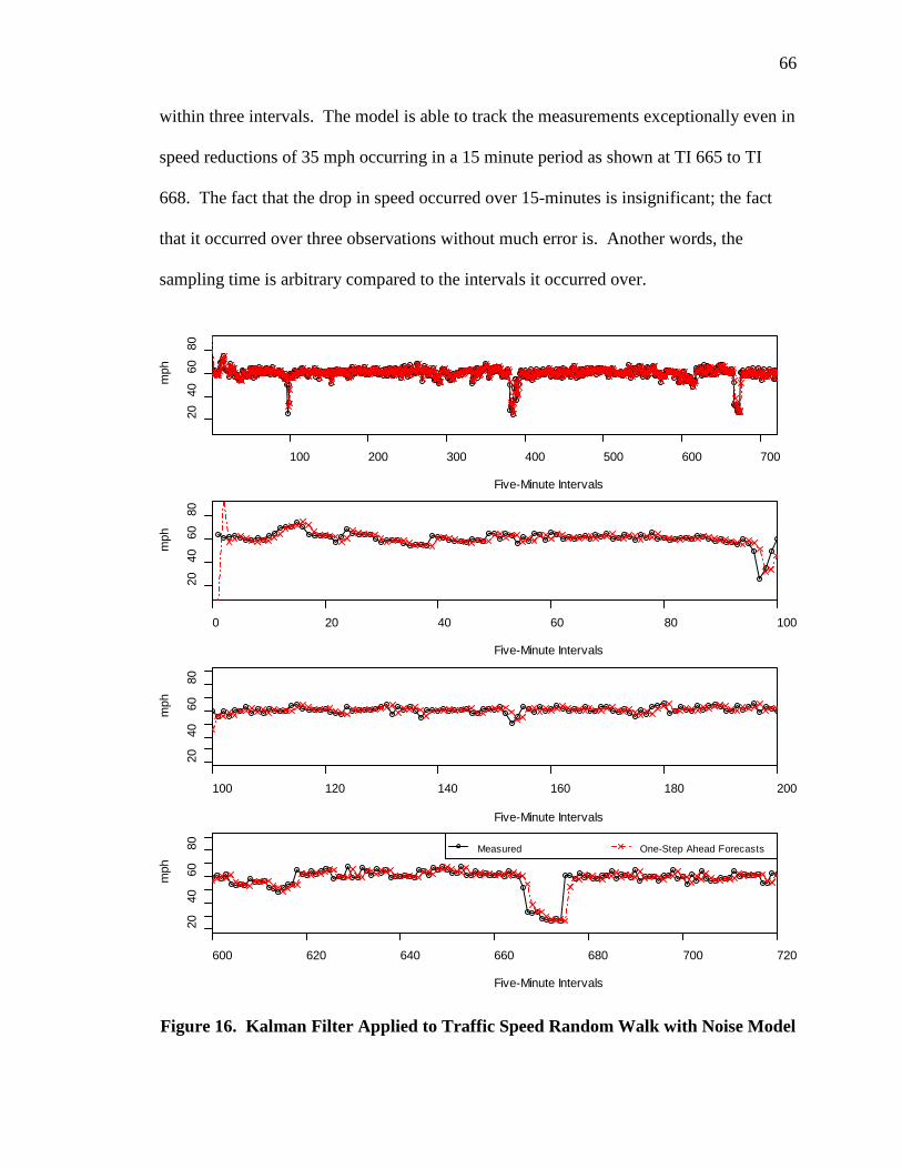
66
within three intervals. The model is able to track the measurements exceptionally even in
speed reductions of 35 mph occurring in a 15 minute period as shown at TI 665 to TI
668. The fact that the drop in speed occurred over 15-minutes is insignificant; the fact
that it occurred over three observations without much error is. Another words, the
sampling time is arbitrary compared to the intervals it occurred over.
Figure 16. Kalman Filter Applied to Traffic Speed Random Walk with Noise Model
Five-Minute Intervals
mph
100 200 300 400 500 600 700
2040
6080
Five-Minute Intervals
mph
0 20 40 60 80 100
2040
6080
Five-Minute Intervals
mph
100 120 140 160 180 200
2040
6080
Five-Minute Intervals
mph
600 620 640 660 680 700 720
2040
6080 Measured One-Step Ahead Forecasts

67
4.3.4 KF Results: Traffic Speeds RW with Seasonal Component Model
The fitted model modspdseas is:
1 0 0 0 0 0 0 0 0 0 0 00 -1 -1 -1 -1 -1 -1 -1 -1 -1 -1 -10 1 0 0 0 0 0 0 0 0 0 00 0 1 0 0 0 0 0 0 0 0 00 0 0 1 0 0 0 0 0 0 0 00 0 0 0 1 0 0 0 0 0 0 00 0 0 0 0 1 0 0 0 0 0 00 0 0 0 0 0 1 0 0 0 0 00 0 0 0 0 0 0 1 0 0 0 00 0 0 0 0 0 0 0 1 0 0 00 0 0 0 0 0 0 0 0 1 0 00 0 0 0 0 0 0 0 0 0 1 0
10.65 0 0 0 0 0 0
=
=
G
W
[ ]
0 0 0 0 00 1 0 0 0 0 0 0 0 0 0 00 0 0 0 0 0 0 0 0 0 0 00 0 0 0 0 0 0 0 0 0 0 00 0 0 0 0 0 0 0 0 0 0 00 0 0 0 0 0 0 0 0 0 0 00 0 0 0 0 0 0 0 0 0 0 00 0 0 0 0 0 0 0 0 0 0 00 0 0 0 0 0 0 0 0 0 0 00 0 0 0 0 0 0 0 0 0 0 00 0 0 0 0 0 0 0 0 0 0 00 0 0 0 0 0 0 0 0 0 0 0
1
1 1 0 0 0 0 0 0 0 0 0 0
[ .48]
=
=
F
V
(4.18)
The Kalman filter recursive algorithm was applied to (4.18) and the results of the one-
step-ahead forecasts are shown in Figure 17. The data was converted into one-hour
intervals, and although not representative of real-world, the goal was to capture any
seasonal patterns that may have existed. Unexpectedly, the signal-to-noise ratio was the
largest, thus the model had the greatest adaptive capabilities of the three speed models.
The signal-to-noise ratios were similar for the RW, with 2.09, and the Fourier-form, with
2.29, models.

68
Figure 17. Kalman Filter Applied to Traffic Speed Random Walk with Seasonal Component Model

69
4.3.5 KF Results: Traffic Speeds RW with Fourier-Form Model
The fitted model modspdTrig is:
1 0 0 0 0 0 0 0 0 0 0 00 0.87 0.5 0 0 0 0 0 0 0 0 00 0.5 0.87 0 0 0 0 0 0 0 0 00 0 0 0.5 0.87 0 0 0 0 0 0 00 0 0 0.87 0.5 0 0 0 0 0 0 00 0 0 0 0 2.8 16 1 0 0 0 0 00 0 0 0 0 1 2.8 16 0 0 0 0 00 0 0 0 0 0 0 0.5 0.87 0 0 00 0 0 0 0 0 0 0.87 0.5 0 0 00 0 0 0 0 0 0 0 0 0.87 0.5 00 0 0 0 0 0 0 0 0 0.5 0.87 00 0 0 0 0
ee
−
−−=
− −−− −
−− −
G
0 0 0 0 0 0 1
9.6 0 0 0 0 0 0 0 0 0 0 00 0 0 0 0 0 0 0 0 0 0 00 0 0 0 0 0 0 0 0 0 0 00 0 0 0 0 0 0 0 0 0 0 00 0 0 0 0 0 0 0 0 0 0 00 0 0 0 0 0 0 0 0 0 0 00 0 0 0 0 0 0 0 0 0 0 00 0 0 0 0 0 0 0 0 0 0 00 0 0 0 0 0 0 0 0 0 0 00 0 0 0 0 0 0 0 0 0 0 00 0 0 0 0 0 0 0 0 0 0 00 0 0 0 0 0 0 0 0 0 0 0
− =
W
[ ][ ]1 1 0 1 0 1 0 1 0 1 0 1
4.20
=
=
F
V
(4.19)
The Kalman filter recursive algorithm was applied to (4.19) using five-minute interval
data and the results of the one-step-ahead forecasts are shown in Figure 18.

70
Figure 18. Kalman Filter Applied to Traffic Speeds Random Walk with Fourier-form Seasonal Component Model Five-Minute Frequency Data
4.4 Results Analysis
The DLMs constructed for the modeling of traffic volume all performed
exceptionally well with Fourier-form seasonal component model having the smallest
standard errors. Two performance indices were used to rank the models: the Root Mean
Square Error of Prediction (RMSEP), calculated as:
Five-Minute Intervals
mph
100 200 300 400 500 600 700
2040
6080
Five-Minute Intervals
mph
0 20 40 60 80 100
2040
6080
Five-Minute Intervals
mph
100 120 140 160 180 200
2040
6080
Five-Minute Intervals
mph
600 620 640 660 680 700 720
2040
6080 Measured One-Step Ahead Forecasts

71
2
1
1 N
kk
RMSEPN =
×= ∑y (4.20)
and the Mean Absolute Deviation (MAD):
1
1k
k
N
NMAD
=
= ∑ y (4.21)
where N is the number of observations, and ỹk is the residual.
The performance statistics for the traffic volume DLMs can be found in Table 4.1.
Table 4.1. DLM Volume Models Performance statistics
Model MAD RMSEP
Random Walk with Noise 7.08 9.74
RW with Seasonal Component 7.64 10.43
RW with Fourier-form 7.59 10.91
As seen in Table 4.1, the RW with noise model performed better than the other two
models. It should be noted that these statistics are not used for any other purposes than
ranking the models among one another.
The performance statistics for the traffic speeds DLMs can be found in Table 4.2.
Table 4.2. DLM Speed Models Performance statistics
Model MAD RMSEP
Random Walk with Noise 3.00 3.19
RW with Seasonal Component 3.53 3.78
RW with Fourier-form 3.70 4.77
As seen in the above table, the RW model performed better than the other two models.

72
The R environment provided a platform to model data from traffic speeds and
traffic volumes. The results from the DLM and KF models were used as the beginning
point for the matrices used in MATLAB, described in the next section. The RW plus
noise traffic and speed models were chosen for this task. The R file, Section_4.2.R, for
the traffic volume DLMs and KF, can be found in Appendix C. The file, Section_4.3.R,
contains the R code for the traffic speed DLMs and KF and can be found in Appendix D.

73
CHAPTER 5: PREDICTION & CONTROL INTEGRATION
This chapter combines, in MATLAB, the Kalman filter algorithm presented in
Section 3.2 with the control logic presented in Section 3.5. The KFs role is to recursively
forecast the traffic state variables to be used in the control scheme. The traffic state can
be represented by variables that describe the state of the freeway system such as traffic
flow, speed, density, or occupancy. The integration of the KF with the ramp meter
control logic completes the ramp meter algorithmic scheme which is proactive to changes
in freeway conditions by controlling a forecasted state.
Numerical implementation of the KF generates numerical errors, even when the
optimal filter is utilized – e.g., due to round-off errors (Bucy & Joseph, 2005). Joseph
(Bucy & Joseph, 2005) suggested a form for the error covariance update that avoids this,
although, at the expense of computational burden, this form was used in our Kalman
filtering routine. The Joseph-form error covariance estimate (a posteriori):
( ) ( )k|k | 1T
k k k k k k k k kT
−= − − +P I K F P I K F K R K (5.1)
where I is and identity matrix with dimensions equal to the length of the observation
matrix (or vector). Equation 5.1 was used in place of the posteriori covariance Equation
3.11 to avoid numerical errors associated with round-off.

74
5.1 Integration Methodology
The KF makes predictions based on the freeway system output (i.e., the state of
the traffic) for each sections density ρi and the on-ramp queue lengths li. The queue
lengths are estimated by the KF because they are used by the state feedback controller in
the calculation of the metered flow ui. Also, there is continuity of inputs and outputs
between algorithms, meaning the output from the KF is feeding the input of the
controller. The KF compares its prediction with the system outputs, obtained from
roadway sensors, and the controller compares its error signal based on the difference in
the KF output and reference signal. The integration of the KF and the control algorithm
is represented in a block diagram in Figure 19.
Figure 19. Kalman Filter and Control System Block Diagram
The error term for the controller is a function of the mainline density ρ and queue
length l. However, since the reference input for the controller is the critical density ρcr
only, the question may arise as to how the controller uses the KFs queue length prediction
in the error calculation and control input. The answer is in the fact that the controller’s
Kalman Filter
Prediction
Freeway System
error e Controller
Roadway Sensors
Output
Sensor noise
Measurable Disturbances qi,
metered flow ui
+

75
state feedback logic calculates the error as a function of the absolute value of (ρcr – ρi)
and the queue length li given by:
1 1 1 2 1
3 2 2 4 2
( ) ( ) ( )
( ) ( )cr
cr
e k w k w l k
w k w l k
ρ ρ
ρ ρ
= − +
+ − + (5.2)
where the queue length is calculated from the difference in measurable disturbances ri
and the controllers output ui, plus the previous time steps queue length. Therefore, the
“state” of the freeway system is used in the feedback loop to adjust the metering rate ui.
Clearly, the weighting factors determine the significance given to the mainline sections or
ramps through (5.2).
The action taken by the controller to adjust the control output based on the error is
proportional-derivative (PD), as described in Section 3.4. The controller’s block diagram
for the PD action is shown in Figure 20.
Figure 20. Proportional-Derivative Controller Action
The integration of the prediction algorithm and control logic can be thought of as
the complete ramp metering algorithmic scheme. The complete ramp meter scheme
includes the detectors that collect traffic data both on the mainline and the on-ramps, the
ramp meter signal actuators, and the algorithmic scheme.
error e System
output input r

76
5.2 MATLAB Programming: Kalman Filter & Extended Kalman Filter
The observation vector consisted of density measurements from EB sites 5 and 6
that were calculated from flow (veh/hr) and speed (mph) measurements. The
measurements recorded at site 5 were assumed to correspond to the density of section 1,
containing the Eagle Road EB loop on-ramp (Ramp 1) as shown in Figure 21. The
measurements recorded at site 6 were assumed to correspond to the density of section 2,
containing the Eagle Road EB on-ramp (Ramp 2). These measurements can be collected
in real-time with roadway detectors, shown below by the blue dashed lines.
Figure 21. Linearized Freeway System with Radar Sensor’s Locations
5.2.1 Kalman Filter
The discrete-time Kalman filter performs the recursive prediction-correction
estimation. The methodology present in Sections 3.2, 4.2, and 4.3 were numerically
programmed into MATLAB. A Kalman filter was conceptualized and programmed as a
“dual-state” estimation algorithm, computing one-step ahead densities at Section 1 and
Section 2 (as shown in Figure 21). One-step ahead refers to the next discrete time k+1
EB Site 4 EB Site 5 EB Site 6
∆x1 ∆x2
q1 q2
Ramp 1 Ramp 2
Section 1 Section 2
r1 r2
u2 u1
Flow in f
Detectors

77
prediction in which some time interval, Δt, has lapsed. The discrete time step from k to
k+1 is usually equal to the sampling time (T) where kT = Δt.
The dual-state Kalman filter matrices were programmed in MATLAB as:
1 00 1
3.7330 00 5.6221
1 00 1
1.1034 00 2.8308
k
k
k
k
= = = =
G
Q
F
R
(5.3)
where Gk is the state design matrix, Qk is the variance of the state noise wk, Fk is the
observation matrix, and Rk is the variance of the observation noise vk. The parameters of
the model were fitted in R using MLE with similar methodology as outlined in Section
4.2.1. The filter was initialized with the following state process matrix x0 and its error
covariance P0:
0
0
2535
15 00 10
= =
x
P (5.4)
The initial state and error matrices (5.4) were estimated from EB site 5 and site 6 radar
data. In MATLAB, the Kalman filter recursions were programmed rather instinctively
with a “for-loop”:

78
( )( )
( ) ( )( )
( ) ( )( )
( ) ( ) ( )( )
3.5
3.6
3.7
3.9
3.10
∗
∗ ∗
∗
∗ ∗ ∗
for ii= 1:length flow5
xpred = G x_hat;
predrho ii,: = xpred :,1 ';
ppred = G pplus G'+Q;
y_hat = meas ii,: '-F xpred;
resid ii,: = y_hat';
K = ppred F' / F ppred F'+ R ;
( ) ( )( ) ( )( )5.1
∗
∗ ∗ ∗ ∗ ∗ ∗
x_hat = xpred+K y_hat;
pplus = eye 2 -K F ppred eye 2 -K F '+K R K';
end
where the equation number in the left margin corresponds to those found herein.
To build a suitable KF, there are four tuning parameters that are determined prior
to the filters implementation (Saha, Goswami, & Ghosh, 2013). These are the initial state
estimate x0 and the three noise covariance matrices: the initial state estimation error
covariance P0, the state noise covariance Qk, and the measurement noise covariance Rk.
Since x0 and P0 change after the first iteration of the algorithm, the state and the
measurement noise covariances Qk, Rk are more critical in tuning. Subsequently, the
covariance Rk can be determined from knowledge of the sensors characteristics so the
state noise covariance Qk is considered to be the most critical tuning parameter (Saha et
al., 2013).
5.2.2 Extended Kalman Filter
The Kalman filter is only optimal under certain conditions. The process being
estimated is assumed to be a linear dynamical system driven by stochastic processes in
the presence of noise. The noise corrupting the system and its measurements are
assumed to be Gaussian, white noise processes, and independent, or not correlated in

79
time. Most processes occurring in the real-world violate one or both of these
assumptions; however, there are justifications in relaxing these assumptions. For
example, if the Gaussian assumption is removed, the Kalman filter can still be the best
minimum error variance filter (Maybeck, 1982).
Other variants of the Kalman filter exist such as the Extended Kalman filter
(EKF), a non-linear estimator. An EKF was constructed where the nonlinear state and
observation models were described by:
( )1 1k k kf − −= +x x w (5.5)
and
( )k k kh= +y x v (5.6)
where f(∙) and h(∙) are nonlinear functions and vk and wk are Gaussian independent white
noise sequences, as in the KF.
The EKF is similar to the KF except that the nonlinear functions f(∙) and h(∙)
cannot be used directly for estimation, instead, their partial derivatives, known as
Jacobian matrices are used. The state and observation matrices are defined by the partial
derivative Jacobians (which are not given in vector notation to distinguish from previous
KF equations) by:
1| 1
1ˆ k k
kfF
− −
−
∂=∂ xx
(5.7)
and

80
| 1ˆ k k
khH
−
∂=∂ xx
(5.8)
The state estimate (a priori):
( )| 1 1| 1ˆ ˆk k k kf− − −=x x (5.9)
Error covariance estimate (a priori):
| 1 -1 1| 1 -1k k k k k k kF F− − −= +P P Q (5.10)
where Fk-1 is the Jacobian of function f(∙) with respect to x.
Measurement innovation (or residual):
( )| 1ˆk kk kh −= −y y x (5.11)
The innovation covariance:
| 1T
k k k kk kH H−= +S P R (5.12)
Kalman filter gain:
1| 1
Tk k k k kH −
−=K P S (5.13)
Updated state estimate (a posteriori):
| | 1ˆ ˆk k k k k k−= +x x K y (5.14)
Updated error covariance estimate (a posteriori):
| | 1 | 1k k k k k k k kH− −= −P P K P (5.15)
The EKF model were initialized with the following state, error covariance, and noise
matrices in MATLAB:

81
[ ]0
0
ˆ 15 5 15 5
3 0 0 00 2 0 00 0 5 00 0 0 4
5 0 0 00 2 0 00 0 15 00 0 0 6
7 0 0 00 8 0 00 0 5 00 0 0 10
T
k
k
=
=
=
=
x
P
Q
R
(5.16)
The first and third parameters for x̂ were approximated from the KF estimated densities.
The second and fourth parameters for x̂, representing queue length, were necessary for
the algorithm to converge and considered a reasonable initial queue length. To determine
the nonlinear function f(⋅) for the state process, a model was determined from
Greenshields et al. (1935) model for speed and the fundamental traffic Equation (3.12):
1,31,2 1,2 1,3
ˆˆ 1rhom
q vf = −
xx (5.17)
where x̂1,3 is the section 1 and section 3 density, from the predicted state vector x̂; vf1,2
and rhom as previously defined. The nonlinear function f(⋅) is achieved by substituting
q1,2 (5.17) into (3.22), and substituting the state vector x̂2,4 in for queue lengths l1,2 into
(3.22), which gives:
( )
( )
1
11 1 1
1
2 1 1
313 2 1 2 3
2
4 2 2
ˆˆ ˆ 1hom
ˆˆˆˆ ˆ ˆ 1
hom 1 homˆ
f
T xx flow vf xx r
x T ramp uT xxx vf x vf xx r r
x T ramp u
=
+ − − ∆ + −
+ − − ∆ − + −
(5.18)

82
where flow1 is the flow f represented in Equation (3.22) with the Jacobian for the state
process (5.18) given by:
11
1 21 2
1 1 rhomrhom 11
1 1 2 2rhom rhomrhom 1 rhom 12
ˆˆ
0 0 00 1 0 0
ˆ ˆˆ ˆ
0 020 0 0 1
T vf vf
L
T vf vf T vf vf
L
F
L
+ −
+ + − −
=
−
xx
x xx x (5.19)
and the Jacobian of the measurement:
1 0 0 00 1 0 00 0 1 00 0 0 1
H
=
(5.20)
As in the KF, the EKFs Q and R matrices determines to a large extent the behavior of the
EKF. Generally, the higher the standard deviation (SD) of the measurement noise
compared to the state noise, the lower the filter gain. A lower filter gain results the
measurements y(k) having a lower impact of on | 1ˆ k k−x and vice versa (Wang &
Papageorgiou, 2005).

83
5.3 MATLAB Programming: Ramp Meter Control Files
The control logic presented in Section 3.5 was coded into MATLAB.
Obviously, traffic jams are unavoidable when traffic exceeds the physical limitations of
the freeway system or external conditions, such as weather or incidents play a role.
In this study, the radar data was collected by lane. However, a general case was
established by considering Lane 1 data only, the right-most lane in to which on-ramps
merge, or to which they are adjacent to. This was a reasonable starting point because it
was assumed most interactions with the on-ramp and freeway section take place at the
interface between the merge or where interactions occurring between them, such as
weaving and merging, are facilitated through.
The ramp meter control files were created in MALAB as separate m-files
(MATLABs file-type). The main file, rampmeter_runfile.m, contains the user inputs:
gain regulator parameters, weighting factors, any other known parameters, and initial
values. This is the main file that “calls” the other files that contain functions:
kalman_pred.m, ramp1_meter.m, and ramp2_meter.m. Functions in MATLAB are
custom programs that accept user inputs and return outputs, created by the user to
perform a specific task. The function kalman_pred.m computes the forecasted system
dynamics for the section density ρi(k+1) and queue length li(k+1). Ramp1_meter.m and
ramp2_meter.m are the on-ramp metering control logic files that controls the release of
vehicles to the mainline freeway. The main file also loads the data containing the radar
measurements at each section (analogous to inductive loop data). The data file contained
measurements for traffic flows f and qi, ramp 1 and 2 demand volumes r1 r2., average
speeds, and the calculated density for sections 1 and 2.

84
The feedback gain parameters, mainline and ramp weighting factors, and other
known parameters are shown in Tables 5.1 through 5.3. The parameters L1, L2, RL1,
and RL2 of Table 5.1 are measurable parameters. The remaining parameters were
determined from the fundamental diagrams of the measured radar data, provided in
Appendix E Figure 42 and Figure 43. Because of relatively few observations in the
congested zone, lanes 1 through 4 were included in those plots.
Table 5.1. Known Parameters for Ramp Meter Run-File
L1 0.298 Length of Freeway Section 1 (mi) L2 0.391 Length of Freeway Section 2 (mi)
RL1 0.38 Length of Ramp 1 EB loop RL2 0.29 Length of Ramp 2 EB On-Ramp rhom 110 Jam Density (veh/mi) rhoc1 33 Critical Density Section 1 (veh/mi) rhoc2 41 Critical Density Section 2 (veh/mi) vf1 75 Free-Flow Speed Section 1 (mph) vf2 62 Free-Flow Speed Section 2 (mph) T 5/60 Time-Step (hr)
Table 5.2. Initial Regulator Gains for Feedback Ramp Meter Control
dcgain 0.40 Decoupled Gain ccgain 0.50 Coupled Gain alpha1 0.65 Distribution Factor Ramp 1 alpha2 0.35 Distribution Factor Ramp 1
Table 5.3. Weighting Factors for Mainline and Ramp Sections
w1 0.35 Mainline Section 1 w2 0.65 Ramp 1 EB Loop w3 0.35 Mainline Section 2 w4 0.65 Ramp 2 EB On-Ramp

85
rampmeter_runfile.m, kalman_pred.m, ramp1_meter.m, and ramp2_meter.m files
can be found in the Appendix A: MATLAB Ramp Meter Control M-Files.
5.4 Simulation: KF & Decoupled Feedback Control Integration
Simulations were run on the decoupled and coupled control logic. The initial
parameters for the decoupled control scheme are shown in Tables 5.1 through 5.3. The
KF one-step-ahead predictions and measured sensor data for section 1 Time Interval (TI)
0 – 500 (where a TI is five-minutes) are shown in Figure 22; TI 500 – 1000 are shown in
Figure 23. The KF one-step-ahead predictions and measured sensor data for section 2, TI
1000 – 1500, are shown in Figure 24; TI 1500 – 2000 are shown in Figure 25. The KF
had excellent results and was able to track the density observations throughout the length
of the simulation.
Figure 22. Kalman Filter Section 1 Density Predictions TI 0–500
0 50 100 150 200 2500
20
40
60Density Section 1
veh/
mi
KF Measured
Dual-State KF
250 300 350 400 450 5000
10
20
30
veh/
mi
Five-minute Intervals
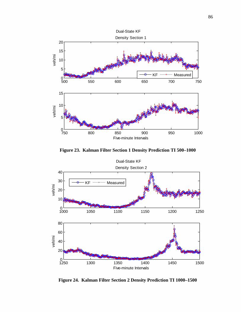
86
Figure 23. Kalman Filter Section 1 Density Prediction TI 500–1000
Figure 24. Kalman Filter Section 2 Density Prediction TI 1000–1500
500 550 600 650 700 7500
5
10
15
20Density Section 1
veh/
mi
KF Measured
Dual-State KF
750 800 850 900 950 10000
5
10
15
veh/
mi
Five-minute Intervals
1000 1050 1100 1150 1200 12500
10
20
30
40Density Section 2
veh/
mi
KF Measured
Dual-State KF
1250 1300 1350 1400 1450 15000
20
40
60
80
veh/
mi
Five-minute Intervals

87
Figure 25. Kalman Filter Section 2 Density Prediction TI 1500–2000
Figure 26. Decoupled Controls: Ramp Demand, Metered Flow, & Queue Length TI 0–1000
1500 1550 1600 1650 1700 17500
20
40
60
80Density Section 2
veh/
mi
KF Measured
Dual-State KF
1750 1800 1850 1900 1950 20000
10
20
30
40
veh/
mi
Five-minute Intervals
0 100 200 300 400 500 600 700 800 900 10000
50
100
150w 1 =0.65, w 2 =0.35, w 3 =0.65, w 4 =0.35, dcgain =0.40
Dem
and
Flow
(veh
/hr)
Ramp 1 Ramp 2
0 100 200 300 400 500 600 700 800 900 10000
50
100
150
Met
ered
Flo
w(v
eh/h
r)
Decoupled Control
0 100 200 300 400 500 600 700 800 900 10000
50
Que
ue L
engt
h(v
eh)
Five-minute Intervals

88
Figure 27. Decoupled Controls: Ramp Demand, Metered Flow, & Queue Length TI1 1000–2000
The initial results with the decoupled gain dcgain set equal to 0.40 are shown in
Figure 26 and Figure 27. Extended queue lengths began forming at approximately TI 0,
TI 295, TI 600, TI 1170, TI 1420, and TI 1720, taking approximately 200 TIs to disperse.
These periods all correspond to morning rush hour.
A performance metric named “Ramp 1, Ramp 2 delay,” displayed at the top of
Figure 27, was developed to assess the controller performance. This metric is simply the
number of observation periods that a queue was present. Since there is no way to
determine timing of individual cars, details of impacts due to queues is impossible in this
setting to calculate, without microsimulation. Ramp 1 experienced more than 1237 of the
2000 total TIs with a queue present. Ramp 2 experienced 379 of the total 2000 TIs with a
queue present. Equally undesirable is the time the controller took to disperse the queue.
1000 1100 1200 1300 1400 1500 1600 1700 1800 1900 20000
50
100
150Ramp 1 delay =1237, Ramp 2 delay=379
Dem
and
Flow
(veh
/hr)
Ramp 1 Ramp 2
1000 1100 1200 1300 1400 1500 1600 1700 1800 1900 20000
50
100
150
Met
ered
Flo
w(v
eh/h
r)
Decoupled Control
1000 1100 1200 1300 1400 1500 1600 1700 1800 1900 20000
50
Que
ue L
engt
h(v
eh)
Five-minute Intervals

89
Although, nothing more than inference can be made, the number of time intervals with a
queue can be viewed as a negative performance metric for comparing different controller
configurations.
The residuals from the KF can be seen in Figure 28 and displays the root mean
square error of the prediction (RMSEP), calculated as:
2| 1
1 ˆk k kN −× −∑ y x (5.21)
where N is the number of observations.
Figure 28. Kalman Filter Section 1 & 2 Residuals
The RMSEP for section 1 was 1.99 (veh/mi) and 2.76 (veh/mi) for section 2. A
performance metrics, RMSEP, was used for criteria for evaluating the tested models.
0 200 400 600 800 1000 1200 1400 1600 1800 2000-20
-10
0
10
20RMSEP Sec 1 = 1.99, Sec 2 = 2.76
Sec
tion
1
Dual-State KF Residuals
0 200 400 600 800 1000 1200 1400 1600 1800 2000-20
-10
0
10
20
Five-minute Intervals
Sec
tion
2

90
What that means is the RMSEP was used only as an indicator of performance of similar
models used in this study. The RMSEP should therefore be viewed as a tuning
parameter. The RMSEP were consequently deemed acceptable with the 5-minute
resolution data.
5.4.1 Decoupled Control Testing
Because the decoupled setting treats the ramp controllers as isolated controllers,
the ramp demand was staggered so that a peak flow would occur at separate times for the
ramps. They can be viewed as two independent on-ramps with their objectives only
sought locally. The ramp 2 demand flows were shifted by approximately 6.7-hours (or
80 TI) to test the controller’s performance when peak demands occurred at different
periods.
Figure 29. Decoupled Results TI 0–1000 for the Shifted Ramp 2 Demands
0 100 200 300 400 500 600 700 800 900 10000
50
100
150w 1 =0.65, w 2 =0.35, w 3 =0.65, w 4 =0.35, dcgain =0.40
Dem
and
Flow
(veh
/hr)
Ramp 1 Ramp 2
0 100 200 300 400 500 600 700 800 900 10000
50
100
150
Met
ered
Flo
w(v
eh/h
r)
Decoupled Control
0 100 200 300 400 500 600 700 800 900 10000
50
Que
ue L
engt
h(v
eh)
Five-minute Intervals

91
Figure 30. Decoupled Results TI 1000–2000 for the Shifted Ramp 2 Demands
The results of the shifted ramp 2 demand are shown in Figure 29 and Figure 30. Ramp 1
experienced less than 100 more periods with a queue present while ramp 2 experienced
only 2 additional periods with a queue.
1000 1100 1200 1300 1400 1500 1600 1700 1800 1900 20000
50
100
150Ramp 1 delay =1342, Ramp 2 delay=390
Dem
and
Flow
(veh
/hr)
Ramp 1 Ramp 2
1000 1100 1200 1300 1400 1500 1600 1700 1800 1900 20000
50
100
150
Met
ered
Flo
w(v
eh/h
r)
Decoupled Control
1000 1100 1200 1300 1400 1500 1600 1700 1800 1900 20000
50
Que
ue L
engt
h(v
eh)
Five-minute Intervals

92
5.5 Simulation: KF & Coupled Feedback Control Integration
The integrated, coupled-control scheme was tested with the parameters given in
Table 5.1 through Table 5.3. The distribution factors were 0.65 for the Loop On-Ramp
and 0.35 for the EB On-Ramp. The values were chosen based on Kachroo and Ozbay,
(2003).
The plots for the ramp demands ri (veh/hr), metered flow ui (veh/hr), and queue
lengths li (veh) for the Loop On-Ramp and EB On-Ramp are shown in Figure 31 and
Figure 32.
Figure 31. Coupled Controls: Ramp Demand, Metered Ramp Flow, & Queue Length TI 0–1000
0 100 200 300 400 500 600 700 800 900 10000
50
100
150w 1 =0.65, w 2 =0.35, w 3 =0.65, w 4 =0.35, ccgain =0.50
Dem
and
Flow
(veh
/hr)
Ramp 1 Ramp 2
0 100 200 300 400 500 600 700 800 900 10000
50
100
150
Met
ered
Flo
w(v
eh/h
r)
Coupled Control alpha1 = 0.65, alpha2 = 0.35
0 100 200 300 400 500 600 700 800 900 10000
20
40
Que
ue L
engt
h(v
eh)
Five-minute Intervals

93
Figure 32. Coupled Controls: Ramp Demands, Metered Ramp Flow, & Queue Length TI 1000–2000
As seen in Figure 31 and Figure 32, the metered flow has much less turbulence than the
unmetered ramp demand. On-ramp queue began forming at approximately TI 1, TI 300,
TI 600, TI 1170, TI 1450, and TI 1750. The time to dissipate the queues were about 200
five-minute periods in all cases. These periods all correspond to morning rush hour.
The above plots reveal that EB on-ramp has periods where its queue formation
exhibits extreme maximum peaks. The parameter w4 was adjusted to 0.45 to give more
weight to the on-ramp queue and the gain ccgain was increased to 0.60; the results can be
seen in Figure 33 and Figure 34.
1000 1100 1200 1300 1400 1500 1600 1700 1800 1900 20000
50
100
150Ramp 1 delay =692, Ramp 2 delay=780
Dem
and
Flow
(veh
/hr)
Ramp 1 Ramp 2
1000 1100 1200 1300 1400 1500 1600 1700 1800 1900 20000
50
100
150
Met
ered
Flo
w(v
eh/h
r)
Coupled Control
1000 1100 1200 1300 1400 1500 1600 1700 1800 1900 20000
10
20
30
Que
ue L
engt
h(v
eh)
Five-minute Intervals

94
Figure 33. Coupled Controls: Adjusted Ramp 2 and Gain Parameters TI 0–1000
Figure 34. Coupled Controls: Adjusted Ramp 2 and Gain Parameters TI 1000–2000
0 100 200 300 400 500 600 700 800 900 10000
50
100
150w 1 =0.65, w 2 =0.35, w 3 =0.55, w 4 =0.45, ccgain =0.60
Dem
and
Flow
(veh
/hr)
Ramp 1 Ramp 2
0 100 200 300 400 500 600 700 800 900 10000
50
100
150
Met
ered
Flo
w(v
eh/h
r)
Coupled Control alpha1 = 0.65, alpha2 = 0.35
0 100 200 300 400 500 600 700 800 900 10000
5
10
15
Que
ue L
engt
h(v
eh)
Five-minute Intervals
1000 1100 1200 1300 1400 1500 1600 1700 1800 1900 20000
50
100
150Ramp 1 delay =332, Ramp 2 delay=534
Dem
and
Flow
(veh
/hr)
Ramp 1 Ramp 2
1000 1100 1200 1300 1400 1500 1600 1700 1800 1900 20000
50
100
150
Met
ered
Flo
w(v
eh/h
r)
Coupled Control
1000 1100 1200 1300 1400 1500 1600 1700 1800 1900 20000
10
20
Que
ue L
engt
h(v
eh)
Five-minute Intervals

95
As seen in the above figures, the extreme peaks of ramp 2’s queue was reduced as well as
the periods a queue was present on ramp 1. The above weighting parameter settings were
repeated with an increased ccgain of 0.95; the results are below in Figure 35 and Figure
36.
Figure 35. Coupled Controls: Adjusted Gain Parameters TI 0–1000
0 100 200 300 400 500 600 700 800 900 10000
50
100
150w 1 =0.65, w 2 =0.35, w 3 =0.55, w 4 =0.45, ccgain =0.95
Dem
and
Flow
(veh
/hr)
Ramp 1 Ramp 2
0 100 200 300 400 500 600 700 800 900 10000
50
100
150
Met
ered
Flo
w(v
eh/h
r)
Coupled Control alpha1 = 0.65, alpha2 = 0.35
0 100 200 300 400 500 600 700 800 900 10000
5
10
15
Que
ue L
engt
h(v
eh)
Five-minute Intervals

96
Figure 36. Coupled Controls: Adjusted Gain Parameters TI 1000–2000
This control configuration had excellent results with ramp 1 experiencing 118
observation periods with a queue present while ramp 2 experienced 306 observation
periods with a queue present. The overall benefits of increasing the gain and establishing
the magnitude will need to be tested in microsimulation.
1000 1100 1200 1300 1400 1500 1600 1700 1800 1900 20000
50
100
150Ramp 1 delay =118, Ramp 2 delay=306
Dem
and
Flow
(veh
/hr)
Ramp 1 Ramp 2
1000 1100 1200 1300 1400 1500 1600 1700 1800 1900 20000
50
100
150
Met
ered
Flo
w(v
eh/h
r)
Coupled Control
1000 1100 1200 1300 1400 1500 1600 1700 1800 1900 20000
10
20
Que
ue L
engt
h(v
eh)
Five-minute Intervals

97
5.6 Simulation: Extended KF Results
The EKF one-step-ahead predictions and measured sensor data for section 1 Time
Interval (TI) 0 – 1000 (where a TI is five-minutes) are shown in Figure 37; TI 1000 –
2000 are shown in Figure 38. The EKF one-step-ahead predictions and measured sensor
data for section 2, TI 0 – 1000, are shown in Figure 39; TI 1000 – 2000 are shown in
Figure 40. The EKF had excellent results and was able to track the density observations
throughout the length of the simulation. The residuals and RMSEP for sections 1 and 2
can be seen in Figure 41.
Figure 37. Extended Kalman Filter Prediction Section 1 Density TI 0–1000
0 50 100 150 200 250 300 350 400 450 5000
10
20
30
40Density Section 1
veh/
mi
EKFMeasured
Extended Kalman Filter
500 550 600 650 700 750 800 850 900 950 10000
5
10
15
20
Five-minute Intervals
veh/
mi

98
Figure 38. Extended Kalman Filter Prediction Section 1 Density TI 1000–2000
Figure 39. Extended Kalman Filter Prediction Section 2 Density TI 0–1000
1000 1050 1100 1150 1200 1250 1300 1350 1400 1450 15000
10
20
30
40Density Section 1
veh/
mi
EKFMeasured
Extended Kalman Filter
1500 1550 1600 1650 1700 1750 1800 1850 1900 1950 20000
10
20
30
40
Five-minute Intervals
veh/
mi
0 50 100 150 200 250 300 350 400 450 5000
10
20
30
40Density Section 2
veh/
mi
EKFMeasured
Extended Kalman Filter
500 550 600 650 700 750 800 850 900 950 10000
10
20
30
Five-minute Intervals
veh/
mi

99
Figure 40. Extended Kalman Filter Prediction Section 2 Density TI 1000–2000
Figure 41. Extended Kalman Filter Prediction Residuals Sections 1 & 2
1000 1050 1100 1150 1200 1250 1300 1350 1400 1450 15000
10
20
30
40Density Section 2
veh/
mi
EKFMeasured
Extended Kalman Filter
1500 1550 1600 1650 1700 1750 1800 1850 1900 1950 20000
10
20
30
Five-minute Intervals
veh/
mi
0 200 400 600 800 1000 1200 1400 1600 1800 2000
-20
-10
0
10
20
Sec
tion
1
RMSEP Section 1 = 4.23, Section 2 = 4.72
EKF Residuals
0 200 400 600 800 1000 1200 1400 1600 1800 2000
-20
-10
0
10
20
Five-minute Intervals
Sect
ion
2
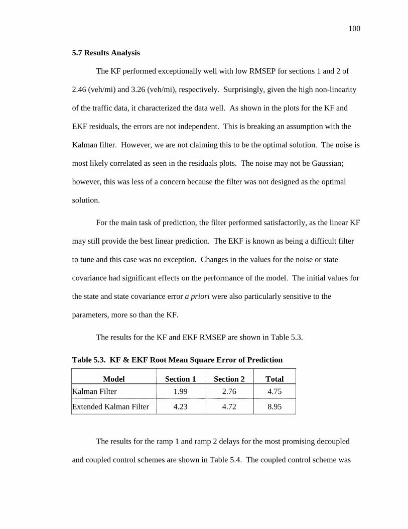
100
5.7 Results Analysis
The KF performed exceptionally well with low RMSEP for sections 1 and 2 of
2.46 (veh/mi) and 3.26 (veh/mi), respectively. Surprisingly, given the high non-linearity
of the traffic data, it characterized the data well. As shown in the plots for the KF and
EKF residuals, the errors are not independent. This is breaking an assumption with the
Kalman filter. However, we are not claiming this to be the optimal solution. The noise is
most likely correlated as seen in the residuals plots. The noise may not be Gaussian;
however, this was less of a concern because the filter was not designed as the optimal
solution.
For the main task of prediction, the filter performed satisfactorily, as the linear KF
may still provide the best linear prediction. The EKF is known as being a difficult filter
to tune and this case was no exception. Changes in the values for the noise or state
covariance had significant effects on the performance of the model. The initial values for
the state and state covariance error a priori were also particularly sensitive to the
parameters, more so than the KF.
The results for the KF and EKF RMSEP are shown in Table 5.3.
Table 5.3. KF & EKF Root Mean Square Error of Prediction
Model Section 1 Section 2 Total Kalman Filter 1.99 2.76 4.75
Extended Kalman Filter 4.23 4.72 8.95
The results for the ramp 1 and ramp 2 delays for the most promising decoupled
and coupled control schemes are shown in Table 5.4. The coupled control scheme was

101
superior to the decoupled; however, simulation and optimization is needed to determine
the optimal settings for the weighting functions and control gain. In a traffic
microsimulation, the stochastic nature of freeway traffic can be simulated, allowing for
the results of a parameter’s adjustment to be observed.
Table 5.4. Decoupled & Coupled Ramp Delays
Model Ramp 1 Delay Ramp 2 Delay Total Decoupled 1237 379 1616
Coupled 118 306 424
In either the decoupled or coupled setting, our metering control logic needs to be
converted to a green-phase duration time for the ramp meter signal. The equation to
convert the metering rate ui(k) to a green phase g is:
( )i
sat
u kg Cu
= (5.22)
where C is the cycle length (sec) and usat is the saturated ramp flow (veh/hr).
When either controller’s distribution factor in the coupled setting is more than 0.65, the
other ramp experiences queue growth at a much faster rate.

102
CHAPTER 6: CONCLUSIONS
With the rapid growth of the Treasure Valley and the distribution of housing and
employment centers, congestion management will be vital as there is an increase in
vehicle miles traveled. An increase in freeway capacity can result in congestion levels
that quickly become similar to those prior to adding the additional capacity. Since new
construction is often the last resort to improve the operations of a freeway, strategies that
are more cost-effective and utilize existing infrastructure or require minimal expansion
are needed to alleviate congestion in the region.
To accomplish this, it is essential to utilize technologies that generate system-
wide improvement. The Ada County Highway District is emphasizing technologies
involving Active Traffic Management, Adaptive Signals, and other Intelligent
Transportation Systems (ITS) (ACHD, 2012). A ramp metering strategy that is
predictive, adaptive, and coordinated aligns with the District’s focus to identify roadway
improvements that plays a role in the development of the Transportation Improvement
Plan, which is the regional mid-range transportation plan developed by COMPASS; and
the Idaho Transportation Investment Plan, the state-level transportation plan developed
by ITD.
I-84 experiences recurring and nonrecurring congestion resulting from bottleneck
formations, especially near the Eagle Road interchange. The Eagle Road interchanges
two East Bound on-ramps experience some of the heaviest traffic volume along I-84.

103
Based on these relationships, a predictive feedback on-ramp metering control strategy,
that is proactive to the onset of congestion breakdown, was developed. The two Eagle
Road EB on-ramps were chosen as test locations for on-ramp metering.
The ramp meter scheme uses a Kalman filter, a recursive forecasting algorithm, to
predict traffic density and estimate on-ramp queue lengths and a feedback control logic to
adjust the metering rate. The adaptive control scheme works by controlling the traffic
density on the mainline while also considering on-ramp queues. Many ramp meter
systems in use today have no sophisticated way to handle queues except through queue
flushing or queue override.
6.1 Summary of Work
A feedback predictive control scheme was designed for two on-ramps at the Eagle
Road interchange on I-84. Radar sensors were installed between the Meridian Road and
Eagle Road interchanges from November 6 through November 15 on the EB side of I-84
and November 20 through November 29 in 2013 on the WB side of I-84. The radar
sensors collected data for traffic volume, average speeds, occupancy, and vehicle
classification. The ramp meter control design was separated into two major research
components: prediction and control.
In the first component, the design of dynamic linear models and Kalman filters,
used for prediction of the state of traffic, was performed in R and MATLAB. The design
of the metering control logic algorithm was performed in MATLAB. Finally, these two
components were combined into a single integrated algorithmic program.

104
6.2 Implementation
The KF appears to be a suitable algorithm for this application. It is a simple,
recursive data processing algorithm with relatively few parameters to tune. The
conversion from ramp metering rate (how many vehicles are allowed to enter the freeway
through the ramp per control interval) to the division of signal cycle (the length of
green/red phase) that actually controls the meter needs to be decided after many
simulations are made in a traffic microsimulation program, such as Vissim (PTV Planug
Trasport Verker AG, 2013). A reasonable minimum cycle is around 4.5 seconds,
obtained by a red time of 2.5 seconds and a green time of 2 seconds. Below in Table 6.1
are the FHWA recommended cycle lengths, approximate range of metering rates, and
capacities of three ramp scenarios.
Table 6.1. FHWA Recommended Cycle Length, Metering Rates, & Associated Capacity
Flow Control Scheme No. of Lanes
Cycle Length
(sec)
Range of Metering
Rates (veh/hr) Capacity (veh/hr)
One Vehicle Per Green 1 4 – 4.5 Seconds 240 – 900 900
Two Vehicles Per Green 1 6 – 6.5 Seconds 240 – 1200 1100 –
1200
Tandem 2 - 400 – 700 1600 – 1700
Section 5.4.1 presented the tuning of the controls; however, this was for
demonstrative purposes only. This is because it is very difficult to analytically determine
these values and the impact they will have on the performance of the ramp metering
control law (Yasar, Ozbay, & Kachroo, 2006).

105
6.3 Recommendations for Future Work
With the construction of the new Meridian Interchange, lanes will be increased to
four, eliminating the effects of a lane drop. This scenario is advantageous for study
because it may have the potential to provide posteriori evidence to the effects of adding
an additional lane to a persistent bottleneck. To demonstrate the true capabilities of the
prediction and control logic, the code will need to be converted into a language like C++
and converted into a .dll. This recommendation is ideal for the Vissim traffic
microsimulation software. The prediction algorithms are ready to test in a controller.
The modelling, testing, and validation has been extensive and successful enough to
warrant the algorithm into a controller for field evaluation.
The METANET traffic model has been shown to accurately represent traffic
under a range of conditions (Papageorgiou, Blosseville, & Haj-Salem, 1990a;
Papageorgiou et al., 1990b; Wang & Papageorgiou, 2005). This traffic model should be
used as the basis for the non-linear equations in the EKF prediction algorithm.
The framework for an integrated predictive and control logic algorithm has been
developed. Simulation and optimization needs to be performed to determine the optimal
settings for the controller and locations the controllers are being implemented. Yasar et
al. (2006) recommends tuning these parameters through a series of multiple
microsimulation runs.

106
REFERENCES
ACHD. (2012). Ada County Highway District Five-Year Work Plan. Boise, ID. Retrieved from http://www.achdidaho.org/Departments/PP/Docs/FYWP/2013-2017/Final_Print_Web_Version.pdf
Adeli, H., & Karim, A. (2005). Wavelets in Intelligent Transportation Systems (1st ed., p. 222). West Sussex, England: John Wiley & Sons.
Aghdashi, S. (2013). Traffic Flow Optimization in a Freeway with Stochastic Segment Capacity. Ph.D. Dissertation, North Carolina State University.
Araki, M. (2002). PID Control. Control Systems, Robotics and Automation, 2. Retrieved from http://www.eolss.net/ebooks/Sample Chapters/C18/E6-43-03-03.pdf
Arnold, E. D. (1998). Report Ramp Metering: A Review of the Literature. Virginia Transportation Research Council (p. 21). Retrieved from http://www.virginiadot.org/vtrc/main/online_reports/pdf/99-TAR5.pdf
Astrom, K. J., & Murray, R. M. (2012). Feedback Systems An Introduction for Scientists and Engineers (2.11b ed.). Woodstock, Oxfordshire, United Kingdom: Princeton University Press. Retrieved from http://www.cds.caltech.edu/~murray/books/AM08/pdf/am08-complete_28Sep12.pdf
Bisen, P. S., & Sharma, A. (2012). Introduction to Instrumentation in Life Sciences. CRC Press.
Bogenberger, K., & May, A. D. (1999). Advanced Coordinated Traffic Responsive Ramp Metering Strategies Klaus Bogenberger. Berkeley, CA.
Brilon, W., Geistefeldt, J., & Regler, M. (2005). Reliability of freeway traffic flow: a stochastic concept of capacity. Proceedings of the 16th International Symposium on Transportation and Traffic Theory, (July), 125–144.
Bucy, R. S., & Joseph, P. D. (2005). Filtering for stochastic processes with applications to guidance. Providence, R.I.: AMS Chelsea Publishing.
Casdagli, M. (1992). A dynamical systems approach to modeling input-output systems. In Santa Fe Institute Studies In The Sciences Of Complexity-Proceedings Volume (Vol. 12, p. 265). Addison-Wesley Publishing Co.

107
Cassidy, M. (2003). Traffic flow and capacity. Handbook of Transportation Science, 1–36. Retrieved from http://www.springerlink.com/index/M504722030H0HR63.pdf
Chu, L., Liu, H. X., Recker, W., & Zhang, H. M. (2004). Performance evaluation of adaptive ramp-metering algorithms using microscopic traffic simulation model. Journal of Transportation Engineering, 130(3), 330–338.
COMPASS. (2011). Communities in Motion Performance Monitoring Report. Meridian, Idaho. Retrieved from http://www.compassidaho.org/documents/prodserv/reports/Board2011PerformanceMonitoringReport.pdf
COMPASS. (2013). I-84 and I-184: Why This Corridor Matters (Vol. 84, p. 2). Meridian, Idaho. Retrieved from http://www.compassidaho.org/documents/prodserv/CIMupdate/corridor_write-up_I84 I184_Feb2013.pdf
COMPASS. (2014). Communities in Motion 2040 (p. 177). Meridian, Idaho: Community Planning Association of Southwest Idaho. Retrieved from http://www.compassidaho.org/documents/prodserv/CIM2040/2014CommentPeriod/Online_EntireDocument.pdf
Doyle, J., Francis, B., & Tannenbaum, A. (1990). Feedback Control Theory. Design, 134, 219. doi:10.1016/0005-1098(86)90018-X
Durbin, J., & Koopman, S. J. (2012). Time series analysis by state space methods. Oxford University Press.
Edara, P. (2010). HCM 2010: Applications.
Elefteriadou, L. (2014). An introduction to traffic flow theory. Retrieved from http://dx.doi.org/10.1007/978-1-4614-8435-6
Elefteriadou, L., Kondyli, A., Washburn, S., Brilon, W., Lohoff, J., Jacobson, L., … Persaud, B. (2011). Proactive Ramp Management under the Threat of Freeway-Flow Breakdown. Procedia - Social and Behavioral Sciences, 16, 4–14. doi:10.1016/j.sbspro.2011.04.424
Fei, X., Lu, C.-C., & Liu, K. (2011). A bayesian dynamic linear model approach for real-time short-term freeway travel time prediction. Transportation Research Part C: Emerging Technologies, 19(6), 1306–1318. doi:http://dx.doi.org/10.1016/j.trc.2010.10.005
FHWA. (2006). Ramp Management Strategies. Ramp Management and Control Handbook Overview. Federal Highway Administration. doi:10.1111/febs.12678

108
Gazis, D., & Liu, C. (2003). Kalman filtering estimation of traffic counts for two network links in tandem. Transportation Research Part B: Methodological, 37(8), 737–745. doi:10.1016/S0191-2615(02)00059-0
Geistefeldt, J., & Brilon, W. (2009). A Comparative Assessment of Stochastic Capacity. In Transportation and Traffic Theory 2009. Springer.
Ghosh, D. (1978). Estimation of Traffic Variables Using a Linear Model of Traffic Flow. Transportation Research Record, 12(6), 395–402.
Gokasar, I., Ozbay, K., & Kachroo, P. (2013). Coordinated Feedback-Based Freeway Ramp Metering Control Strategies “ C-MIXCROS and D-MIXCROS ” that Take Ramp Queues into Account. In Advances in Dynamic Network Modeling in Complex Transportation Systems (pp. 67–87). Springer, Dordrecht. doi:10.1007/978-1-4614-6243-9
Greenshields, B. D., Channing, W., & Millier, H. (1935). A study of traffic capacity. In Highway research board proceedings (Vol. 1935). National Research Council (USA), Highway Research Board.
Haboian, K. (1993). Freeway Management Strategies (p. 157). Retrieved from http://www.pbworld.com/pdfs/publications/monographs/haboian.pdf
Idaho Department of Labor. (2013). Boise Metro Trends. Retrieved from http://labor.idaho.gov/publications/lmi/pubs/BoiseMSAprofile.pdf
ITD. (2012). District Three Traffic Flow Map. Retrieved from https://itd.idaho.gov/highways/roadwaydata/RTFmaps/2012/AADT_Dist3_2012.pdf
Jacobson, L. N., Henry, K. C., & Mehyar, O. (1989). Real-time metering algorithm for centralized control.
Jia, A. (2013). Stochastic Capacity at Freeway Bottlenecks with Application to Travel Time Prediction. Ph.D. Dissertation, North Carolina State University.
Kachroo, P., & Ozbay, K. (2003). Feedback Ramp Metering in Intelligent Transportation Systems (p. 333). New York, New York: Kluwer Academic / Plenum Publishers.
Kalman, R. E. (1960). A new approach to linear filtering and prediction problems. Journal of Basic Engineering, 82(1), 35–45.
Kaplan, E. E. L., & Meier, P. (1958). Nonparametric estimation from incomplete observations. Journal of the American Statistical Association, 53(282), 457–481. Retrieved from http://www.tandfonline.com/doi/abs/10.1080/01621459.1958.10501452

109
Levinson, D., Zhang, L., Das, S., & Sheikh, A. (2004). Measuring the Equity and Efficiency of Ramp Meters. . Minnesota Department of Transportation.
Lighthill, M. J., & Whitham, G. B. (1955). On kinematic waves. II. A theory of traffic flow on long crowded roads. Proceedings of the Royal Society of London. Series A. Mathematical and Physical Sciences, 229(1178), 317–345.
Lipp, L. E., Corcoran, L. J., & Hickman, G. A. (1991). Benefits of central computer control for Denver ramp-metering system.
Masher, D. P., Ross, D. W., Wong, P. J., Tuan, P. L., Zeidler, H. M., & Petracek, S. (1975). Guidelines for design and operation of ramp control systems.
MATLAB. (2013). MATLAB. Natick, Massachusetts: The MathWorks Inc.
Maybeck, P. S. (1982). Stochastic models, estimation, and control (Vol. 3). Access Online via Elsevier.
Meldrum, D. R., & Taylor, C. E. (1995). Freeway Traffic Data Prediction Using Artificial Neural Networks And Development Of A Fuzzy Logic Ramp Metering Algorithm. Final Technical Report.
Minderhoud, M. M., Botma, H., & Bovy, P. H. L. (1997). Assessment of roadway capacity estimation methods. Transportation Research Record: Journal of the Transportation Research Board, 1572(1), 59–67.
Ojeda, L. L., Kibangou, A. Y., & Wit, C. C. De. (2013). Adaptive Kalman Filtering for Multi-Step ahead Traffic Flow Prediction. American Control Conference. Retrieved from http://hal.inria.fr/docs/00/84/26/84/PDF/ACC_2013_2.pdf
Okutani, I., & Stephanedes, Y. J. (1984). Dynamic prediction of traffic volume through Kalman filtering theory. Transportation Research Part B: Methodological. doi:10.1016/0191-2615(84)90002-X
Paesani, G., Kerr, J., Perovich, P., & Khosravi, F. E. (1997). System wide adaptive ramp metering (SWARM). In Merging the Transportation and Communications Revolutions. Abstracts for ITS America Seventh Annual Meeting and Exposition.
Papageorgiou, M., Blosseville, J.-M., & Hadj-Salem, H. (1990a). Modelling and real-time control of traffic flow on the southern part of Boulevard Périphérique in Paris: Part I: Modelling. Transportation Research Part A: General, 24(5), 345–359.
Papageorgiou, M., Blosseville, J.-M., & Haj-Salem, H. (1990b). Modelling and real-time control of traffic flow on the southern part of Boulevard Périphérique in Paris: Part II: Coordinated on-ramp metering. Transportation Research Part A: General, 24(5), 361–370.

110
Papageorgiou, M., Hadj-Salem, H., & Blosseville, J.-M. (1991). ALINEA: A local feedback control law for on-ramp metering. Transportation Research Record, (1320).
Papageorgiou, M., Hadj-Salem, H., & Middelham, F. (1997). ALINEA local ramp metering: Summary of field results. Transportation Research Record: Journal of the Transportation Research Board, 1603(1), 90–98.
Papageorgiou, M., & Kotsialos, A. (2002). Freeway ramp metering: an overview. IEEE Transactions on Intelligent Transportation Systems, 3(4), 271–281. doi:10.1109/TITS.2002.806803
Petris, G. (2009). dlm: an R package for Bayesian analysis of Dynamic Linear Models. University of Arkansas. Retrieved from ftp://ftp.math.ethz.ch/sfs/pub/Software/R-CRAN/web/packages/dlm/vignettes/dlm.pdf
Petris, G. (2010). An R package for dynamic linear models. Journal of Statistical Software, 36(12), 1–16. Retrieved from http://cran.r-project.org/package=dlm
Petris, G., Petrone, S., & Campagnoli, P. (2009). Dynamic Linear Models With R. Dynamic Linear Models with R (pp. 31–84). Springer. doi:10.1007/b135794
Portugais, B., & Khanal, M. (2014). State-Space Models with Kalman Filtering for Freeway Traffic Forecasting. In Proceedings of The 2014 IAJC/ISAM Joint International Conference. Orlando, FL.
PTV Planug Trasport Verker AG. (2013). PTV VISSIM 6 User Manual. Karlsruhe, Germany.
R Core Team. (2013). R: A language and environment for statistical computing. Vienna, Austria: R Foundation for Statistical Computing. Retrieved from http://www.r-project.org
Saha, M., Goswami, B., & Ghosh, R. (2013). Two Novel Metrics for Determining the Tuning Parameters of the Kalman Filter. Kolkata, India.
Sajjadi, S. S. (2013). Investigating Impact of Sources of Non-recurrent Congestion on Freeway Facilities. Ph.D. Dissertation, North Carolina State University.
Schrank, D., Eisele, B., & Lomax, T. (2012). 2012 Urban Mobility Report.
Schrank, D., & Lomax, T. (2004). THE 2004 Urban Mobility Report. Retrieved from http://lyle.smu.edu/emis/cmmi5/Ibarra/DeskTop/White_Papers/Mobility/Reports/Mobility_Report_2004.pdf

111
Shumway, R. H., & Stoffer, D. S. (2011). Time series analysis and its applications: with R examples. Springer.
Simrock, S. (2007). Control Theory. Proceedings of the CERN Accelerator School on Digital Signal Processing. Retrieved from http://cds.cern.ch/record/1100534/files/p73.pdf?version=1
Smaragdis, E., & Papageorgiou, M. (2003). A Series of New Local Ramp Metering Strategies. Transportation Research Board 82nd Annual Meeting. Retrieved from http://www.ltrc.lsu.edu/TRB_82/TRB2003-001171.pdf
Smaragdis, E., Papageorgiou, M., & Kosmatopoulos, E. (2004). A flow-maximizing adaptive local ramp metering strategy. Transportation Research Part B: Methodological, 38(3), 251–270. Retrieved from http://www.sciencedirect.com/science/article/pii/S0191261503000122
Stephanedes, Y. J. (1994). Implementation of On-Line Zone Control Strategies for Optimal Ramp Metering in the Minneapolis Ring Road. In Road Traffic Monitoring and Control, 1994., Seventh International Conference on (pp. 181–184). IET.
Tampere, C. M. J., & Immers, L. H. (2007). An Extended Kalman Filter Application for Traffic State Estimation Using CTM with Implicit Mode Switching and Dynamic Parameters. 2007 IEEE Intelligent Transportation Systems Conference, 209–216. doi:10.1109/ITSC.2007.4357755
Transportation Research Board, N. A. (2010). Highway Capacity Manual. Washington, D.C.: Transportation Research Board, National Research Council. Retrieved from http://www.hcm2010.org/
US Census. (2012). Census Report. Retrieved from http://www.census.gov/popest/data/cities/totals/2012/files/SUB-EST2012_16.csv
Van Hinsbergen, C. P. I. J., Schreiter, T., Zuurbier, F. S., van Lint, J. W. C., & van Zuylen, H. J. (2012). Localized Extended Kalman Filter for Scalable Real-Time Traffic State Estimation. IEEE Transactions on Intelligent Transportation Systems, 13(1), 385–394. doi:10.1109/TITS.2011.2175728
Wang, Y., & Papageorgiou, M. (2005). Real-time freeway traffic state estimation based on extended Kalman filter: a general approach. Transportation Research Part B: Methodological, 39(2), 141–167. doi:10.1016/j.trb.2004.03.003
Wang, Y., Papageorgiou, M., & Messmer, A. (2008). Real-time freeway traffic state estimation based on extended Kalman filter: Adaptive capabilities and real data testing. Transportation Research Part A: Policy and Practice, 42(10), 1340–1358. doi:http://dx.doi.org/10.1016/j.tra.2008.06.001

112
Wang, Y., Papageorgiou, M., Messmer, A., Coppola, P., Tzimitsi, A., & Nuzzolo, A. (2009). An adaptive freeway traffic state estimator. Automatica, 45(1), 10–24. doi:http://dx.doi.org/10.1016/j.automatica.2008.05.019
Welch, G., & Bishop, G. (2006). An Introduction to the Kalman Filter. In Practice, 7(1), 1–16. doi:10.1.1.117.6808
Wu, X., Michalopoulos, P., & Liu, H. X. (2010). Stochasticity of freeway operational capacity and chance-constrained ramp metering. Transportation Research Part C: Emerging Technologies, 18(5), 741–756. doi:10.1016/j.trc.2009.08.003
Yasar, I., Ozbay, K., & Kachroo, P. (2006). Evaluation of new coordinated feedback-based freeway ramp metering strategy using macroscopic and microscopic simulation models. Applications of Advanced Technology in Transportation : Proceedings of the Ninth International Conference., 798–803.
Yin, Y. Y. Y., Liu, H. L. H., & Benouar, H. (2004). A Note on Equity of Ramp Metering. Proceedings. The 7th International IEEE Conference on Intelligent Transportation Systems (IEEE Cat. No.04TH8749). doi:10.1109/ITSC.2004.1398950
Yoshino, T., Sasaki, T., & Hasegawa, T. (1995). The Traffic-Control System on the Hanshin Expressway. Interfaces, 25(1), 94–108.
Zhang, M., Kim, T., Nie, X., Jin, W., Chu, L., & Recker, W. (2001). Evaluation of On-Ramp Control Algorithms (No. UCB-ITS-PRR-2001-36). Berkeley, CA. Retrieved from http://escholarship.org/uc/item/83n4g2rq.pdf

113
APPENDIX A: MATLAB RAMP METER CONTROL M-FILES
rampmeter_runfile.m
% Main File to Run Feedback Ramp Meter Controls with Dual-State KF and
% Decoupled or Coupled Control Schemes
% Data is stochastically Generated Each Run, Based on Observed Data and a
% Moving Average Random Process
% Regulator Gains
% dcgain: decoupled gain control
% ccgain:coupled gain for ramp
% alpha1:distribution factor ramp 1
% alpha2:distribution factor ramp 2
% Weighting factors
% w1:weight given to mainline section 1
% w2:weight given to ramp 1 EB loop on-ramp
% w3:weight given to mainline section 2
% w4:weight given to ramp 2 EB on-ramp
clear; clc;
global rhom rhoc1 rhoc2 vf1 vf2 T flow5 ramp1 ramp2 flow4new ...
alpha1 alpha2 dcgain ccgain w1 w2 w3 w4 L1 L2 RL1 RL2 ...
G H Q R ii m c meas pplus x_hat resids queue ramp1new ramp2new...
err RMSEP rampdelay TT uvar1 uvar2
load('rampmeter_wrkspc.mat')
% Input parameters
% c = input('Decoupled D-Mixcros(1), Coupled C-Mixcros(2));
c=2;
% Regulator Gains and Weighting Parameters
dcgain=0.90;
ccgain=0.95;
alpha1=0.55;
alpha2=0.45;
w1=.65;
w2=.35;
w3=.65;
w4=.35;
% Known parameters
L1=0.298; % Length of Freeway Section 1 (mi)

114
L2=0.391; % Length of Freeway Section 2 (mi)
RL1=0.38; % Length of Ramp 1 EB Loop
RL2=0.29; % Length of Ramp 2 EB On-Ramp
rhom=110; % Jam Density (veh/mi)
rhoc1=33; % Critical Density section 1 (veh/mi)
rhoc2=41; % Critical Density section 2 (veh/mi)
vf1=73; % free flow speed section 1 (mi/hr)
vf2=62; % free flow speed section 2 (mi/hr)
T=5/60; % Time step
% Kalman Filter design
% State matrix
G = [1 0
0 1];
% State noise
Q = [3.7330 0
0 5.6221];
% Observation matrix
H = [1 0
0 1];
% Observation noise
R = [1.1034 0;
0 2.8308];
% Initial state and error
x0 = [25; 35]; % initial densities
P0 = diag([15 10]);
x_hat = G*x0;
pplus = G*P0*G'+Q;
% Prealocate
m=length(flow5);
X=zeros(m,length(x0));
uvar1=zeros(m,1);
uvar2=zeros(m,1);
ramp1new=zeros(m,1);
ramp2new=zeros(m,1);
flow4new=zeros(m,1);
queue=zeros(m,2);
resids=zeros(m,2);
err=zeros(m,2);
% Begin Ramp Meter Prediction & Control Algorithm
meas=[rho1(1) rho2(1)];
for ii=1:m-1;
% Stochastic Inflow, Ramp 1 and Ramp 2 Volumes
ramp1new(ii)=ramp1(ii)+(.95+.10.*rand(1)).*(ramp1(ii));
ramp2new(ii)=ramp2(ii)+(.95+.10.*rand(1)).*(ramp2(ii));
flow4new(ii)=flow4(ii)+(.95+.10.*rand(1)).*(flow4(ii));
k=feval('kalman_pred')';

115
X(ii,:)=k;
input=[k(1),queue(ii,1),k(2),queue(ii,2)];
uvar1(ii)=ramp1_meter(ii,input);
uvar2(ii)=ramp2_meter(ii,input);
meas(ii+1,:)=[rho1(ii)+(T)*uvar1(ii), rho2(ii)+(T)*uvar2(ii)];
if (X(ii,1)<0), % Variable Constraints
X(ii,1)=0;
end
if (X(ii,1)>rhom),
X(ii,1)=rhom;
end
if (X(ii,2)<0),
X(ii+1,2)=0;
end
if (X(ii,2)>rhom),
X(ii,2)=rhom;
end
if (queue(ii,1)<0),
queue(ii,1)=0;
end
if (queue(ii,2)<0),
queue(ii,2)=0;
end
queue(ii+1,:)=[(queue(ii,1)+T*(ramp1new(ii)-uvar1(ii))),...
(queue(ii,2)+T*(ramp2new(ii)-uvar2(ii)))];
end
rampdelay = (sum(queue>0));
% Root mean square prediction error (RMSEP)
RMSEP=sqrt((1/length(flow5))*sum(abs(resids).^2));
rho1res=meas(:,1)-X(:,1); % Store the Residuals
rho2res=meas(:,2)-X(:,2); % Store the Residuals
rho1pred=X(:,1); % Store the Prediction Section 1
rho2pred=X(:,2); % Store the Prediction Section 2
rho1new=meas(1:end,1); % Store the new Density Section 1
rho2new=meas(1:end,2); % Store the new Density Section 2
TT=1:m; % Time for plots
if c == 1
c='Decoupled Control';
Decoupled_Plots
% Writes results to Excel
D=[dcgain,rampdelay(1),rampdelay(2),w1,w2,w3,w4];
dlmwrite('Deoupled_Tune.csv',D,'-append', 'delimiter', ',');
end
if c == 2
c='Coupled Control';
Coupled_Plots

116
% Writes results to Excel
D=[ccgain,alpha1,alpha2,rampdelay(1),rampdelay(2),w1,w2,w3,w4];
dlmwrite('Coupled_Tune.csv',D,'-append', 'delimiter', ',');
end
% Plot the results
% Control Variable TI 0-1000
figure
subplot(311)
set(gca,'FontSize',9); set(gcf,'Color','White');
plot(TT,ramp1,TT,ramp2,'r-','linewidth',.02);
title(sprintf('w1 =%2.2f, w2 =%2.2f, w3 =%2.2f, w4 =%2.2f, dcgain =%2.2f',...
w1,w2,w3,w4,dcgain));
legend('Ramp 1','Ramp 2','Location',...
'Best','Orientation','horizontal');
ylabel('Flows (veh/hr)');
ylim([0 150])
xlim([0 1000])
hold on
subplot(312)
plot(TT,uvar1,TT,uvar2,'r-');
set(gca,'FontSize',9); set(gcf,'Color','White');
ylabel('Metered flow (veh/hr)');
xlim([0 1000])
ylim([0 150])
hold on
subplot(313)
plot(TT,queue(2:end,1),'-',TT,queue(2:end,2),'r-');
ylabel('Queue Length'); xlabel('Five-minute Intervals');
xlim([0 1000])
ylim([0 20])
set(gca,'FontSize',9); set(gcf,'Color','White');
h=suptitle(sprintf('%s',c));% \n alpha1 = %2.2f, alpha2 = %2.2f',c));%,alpha1,alpha2));
set(h,'FontSize',10,'FontWeight','normal');
set(gca,'FontSize',9); set(gcf,'Color','White');
hold off
% Control Variable TI 1000-2000
figure
subplot(311);
set(gca,'FontSize',8); set(gcf,'Color','White');
plot(TT,ramp1,TT,ramp2,'r-','linewidth',.02);
title(sprintf('Ramp 1 delay =%2.0f, Ramp 2 delay=%2.0f',...
rampdelay(1),rampdelay(2)));
legend('Ramp 1','Ramp 2','Location',...
'Best','Orientation','horizontal');
ylabel('Flows (veh/hr)');
xlim([1000 2000])
ylim([0 150])
hold on
subplot(312)
plot(TT,uvar1,TT,uvar2,'r-');
set(gca,'FontSize',8); set(gcf,'Color','White');
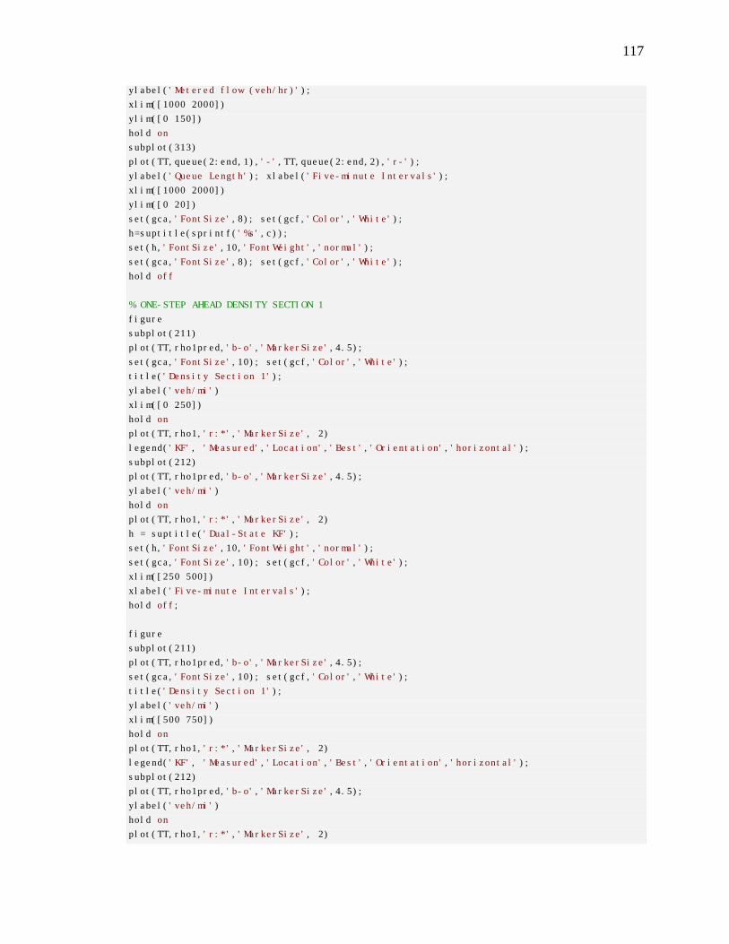
117
ylabel('Metered flow (veh/hr)');
xlim([1000 2000])
ylim([0 150])
hold on
subplot(313)
plot(TT,queue(2:end,1),'-',TT,queue(2:end,2),'r-');
ylabel('Queue Length'); xlabel('Five-minute Intervals');
xlim([1000 2000])
ylim([0 20])
set(gca,'FontSize',8); set(gcf,'Color','White');
h=suptitle(sprintf('%s',c));
set(h,'FontSize',10,'FontWeight','normal');
set(gca,'FontSize',8); set(gcf,'Color','White');
hold off
% ONE-STEP AHEAD DENSITY SECTION 1
figure
subplot(211)
plot(TT,rho1pred,'b-o','MarkerSize',4.5);
set(gca,'FontSize',10); set(gcf,'Color','White');
title('Density Section 1');
ylabel('veh/mi')
xlim([0 250])
hold on
plot(TT,rho1,'r:*','MarkerSize', 2)
legend('KF', 'Measured','Location','Best','Orientation','horizontal');
subplot(212)
plot(TT,rho1pred,'b-o','MarkerSize',4.5);
ylabel('veh/mi')
hold on
plot(TT,rho1,'r:*','MarkerSize', 2)
h = suptitle('Dual-State KF');
set(h,'FontSize',10,'FontWeight','normal');
set(gca,'FontSize',10); set(gcf,'Color','White');
xlim([250 500])
xlabel('Five-minute Intervals');
hold off;
figure
subplot(211)
plot(TT,rho1pred,'b-o','MarkerSize',4.5);
set(gca,'FontSize',10); set(gcf,'Color','White');
title('Density Section 1');
ylabel('veh/mi')
xlim([500 750])
hold on
plot(TT,rho1,'r:*','MarkerSize', 2)
legend('KF', 'Measured','Location','Best','Orientation','horizontal');
subplot(212)
plot(TT,rho1pred,'b-o','MarkerSize',4.5);
ylabel('veh/mi')
hold on
plot(TT,rho1,'r:*','MarkerSize', 2)

118
h = suptitle('Dual-State KF');
set(h,'FontSize',10,'FontWeight','normal');
set(gca,'FontSize',10); set(gcf,'Color','White');
xlim([750 1000])
xlabel('Five-minute Intervals');
hold off;
% ONE-STEP AHEAD DENSITY SECTION 2
figure;
subplot(211)
plot(TT,rho2pred,'b-o','MarkerSize',4.5);
set(gca,'FontSize',10); set(gcf,'Color','White');
title('Density Section 2');
hold on
ylabel('veh/mi')
xlim([1000 1250])
hold on
plot(TT,rho2,'r:*','MarkerSize', 2);
legend('KF', 'Measured','Location','Best','Orientation','horizontal');
subplot(212)
plot(TT,rho2pred,'b-o','MarkerSize',4.5);
hold on
plot(TT,rho2,'r:*','MarkerSize', 2);
h = suptitle('Dual-State KF');...
set(h,'FontSize',10,'FontWeight','normal');
set(gca,'FontSize',10); set(gcf,'Color','White');
ylabel('veh/mi')
xlim([1250 1500])
xlabel('Five-minute Intervals');
hold off;
figure;
subplot(211)
plot(TT,rho2pred,'b-o','MarkerSize',4.5);
set(gca,'FontSize',10); set(gcf,'Color','White');
title('Density Section 2');
hold on
ylabel('veh/mi')
xlim([1500 1750])
hold on
plot(TT,rho2,'r:*','MarkerSize', 2);
legend('KF', 'Measured','Location','Best','Orientation','horizontal');
subplot(212)
plot(TT,rho2pred,'b-o','MarkerSize',4.5);
hold on
plot(TT,rho2,'r:*','MarkerSize', 2);
h = suptitle('Dual-State KF');...
set(h,'FontSize',10,'FontWeight','normal');
set(gca,'FontSize',10); set(gcf,'Color','White');
ylabel('veh/mi')
xlim([1750 2000])
xlabel('Five-minute Intervals');
hold off;

119
% Residuals
figure
subplot(211)
plot(TT,resids(:,1),'-');
set(gca,'FontSize',10); set(gcf,'Color','White');
title(sprintf('RMSEP Sec 1 = %2.2f, Sec 2 = %2.2f',...
RMSEP(1),RMSEP(2)));
hold on
ylabel('Section 1');
xlim([0 2000])
hold on
subplot(212)
plot(TT,resids(:,2),'-')
xlabel('Five-minute Intervals'); ylabel('Section 2')
set(gca,'FontSize',9); set(gcf,'Color','White');
h=suptitle('Dual-State KF Residuals');
set(h,'FontSize',10,'FontWeight','normal');
set(gca,'FontSize',10); set(gcf,'Color','White');
xlim([0 2000])

120
ramp1_meter.m
function u1 = ramp1_meter(t,x)
% Ramp 1 Metered Outflow
global c rhoc1 rhoc2 rhom vf1 vf2 flow4new w1 w2 w3 w4 L1 L2 RL1 RL2...
dcgain ccgain alpha1 T queue ramp1new ramp2new err
q1out=vf1*x(1)*(1-(x(1)/rhom)); % flow out section 1
q2out=vf2*x(3)*(1-(x(3)/rhom)); % flow out section 2
% Decoupled Coordinated Control
% D-MIXCROS
if c == 1
F1=w1*sign((x(1)-rhoc1)+(T/L1)*(-q1out+flow4new(t)))+...
w2*(x(2)+(T/RL1)*ramp1new(t)); % (veh/mi)
G1=(sign(x(1)-rhoc1)*w1*(T/L1)-w2*(T/RL1))^-1; % (mi/hr)
e = w1*abs(x(1)-rhoc1) + w2*abs(x(2)); % (veh/mi)
err(t,1)=e; % store error
u1 = max(0,(-F1-dcgain*e)*G1); % (veh/hr)
% Coupled Distributed Coordinated Control
% C-MIXCROS
elseif c == 2
F1=w1*sign((x(1)-rhoc1)+(T/L1)*(-q1out+flow4new(t)))+...
w2*(x(2)+(T/RL1)*ramp1new(t));
F2=w3*sign((x(3)-rhoc2)+(T/L2)*(-q2out+q1out))+...
w4*(x(4)+T/RL2*ramp2new(t));
F=F1+F2; % (veh/mi)
G1=(sign(x(1)-rhoc1)*w1*(T/L1)-w2*(T/RL1))^-1; % (mi/hr)
e = w1*abs(x(1)-rhoc1)+w2*abs(x(2))+...
w3*abs(x(3)-rhoc2)+w4*abs(x(4)); % (veh/mi)
err(t,2)=e; % store error
u1 = max(0,(G1*(alpha1*(-F-ccgain*e)))); % (veh/hr)
if queue(t,1) <= 0
if ramp1new(t) < u1
u1 = ramp1new(t);
end
end
if x(1) > rhom
u1 = 0;
end
% Ramp Meter Off
else
u1=ramp1new(t);
end

121
ramp2_meter.m
function u2 = ramp2_meter(t,x)
% Ramp 2 Metered Outflow
global c rhoc1 rhoc2 rhom vf1 vf2 flow4new w1 w2 w3 w4 L1 L2 RL1 RL2...
dcgain ccgain alpha2 T queue ramp1new ramp2new err
q1out=vf1*x(1)*(1-(x(1)/rhom)); % flow out section 1
q2out=vf2*x(3)*(1-(x(3)/rhom)); % flow out section 2
% Decoupled Coordinated Control
% D-MIXCROS
if c == 1
F2=w3*sign((x(3)-rhoc2)+(T/L2)*(-q2out+q1out))+...
w4*(x(4)+T/RL2*ramp2new(t)); % (veh/mi)
G2=(sign(x(3)-rhoc2)*w3*(T/L2)-w4*(T/RL2))^-1; % (mi/hr)
e = w3*abs(x(3)-rhoc2) + w4*abs(x(2)); % (veh/mi)
err(t,2)=e; % store error
u2 = max(0,(-F2-dcgain*e)*G2); % (veh/hr)
% Coupled Distributed Coordinated Control
% C-MIXCROS
elseif c == 2
F1=w1*sign((x(1)-rhoc1)+(T/L1)*(-q1out+flow4new(t)))+...
w2*(x(2)+(T/RL1)*ramp1new(t));
F2=w3*sign((x(3)-rhoc2)+(T/L2)*(-q2out+q1out))+...
w4*(x(4)+T/RL2*ramp2new(t));
F=F1+F2; % (veh/mi)
G2=(sign(x(3)-rhoc2)*w3*(T/L2)-w4*(T/RL2))^-1; % (mi/hr)
e = (w1*abs(x(1)-rhoc1)+w2*abs(x(2))+...
w3*abs(x(3)-rhoc2)+w4*abs(x(4))); % (veh/mi)
err(t,2)=e; % store error
u2 = max(0,(G2*(alpha2*(-F-ccgain*e)))); % (veh/hr)
if queue(t,2) <= 0
if ramp2new(t) < u2
u2 = ramp2new(t);
end
end
if x(3) > rhom
u2 = 0;
end
% Ramp Meter Off
else
u2=ramp2new(t);
end

122
kalman_pred.m
function [predrho] = kalman_pred
% Kalman Filter for density prediction sections 1 & 2 using measured
% flows & speeds from EBS5 and EBS6
global meas F H Q R ii pplus x_hat resids
% Filter
xpred = G*x_hat; % eq (3.5)
predrho=[xpred(1); xpred(2)]; % store predictions
ppred = G*pplus* G '+Q; % eq (3.6)
y_hat = meas(ii,:)' - F*xpred; % eq (3.7) Innovation
resids(ii,:)=y_hat'; % store residual
K = (ppred*F')/(F*ppred*F'+ R); % eq (3.9) Kalman Gain
x_hat = xpred + K*y_hat; % eq (3.10)
pplus =(eye(2)-K*F)*ppred*(eye(2)-K*F)'+ K*R*K'; % eq (5.1) (Joseph form)

123
APPENDIX B: EXTENDED KALMAN FILTER MATLAB M-FILE
EKF.m
% Extended Kalman Filter for Density Predictions
clear; clc;
global xhat Q R P flow5 vf1 vf2 L1 L2 rhom1 rhom2
load('rampmeter_wrkspc.mat')
% Known Parameters
L1=0.298; % length of freeway section 1 (mi)
L2=0.391; % length of freeway section 2 (mi)
rhom1=85; % Jam Density section 1 (veh/mi)
rhom2=105; % Jam Density section 2 (veh/mi)
rhoc1=32; % Critical Density section 1 (veh/mi)
rhoc2=24; % Critical Density section 2 (veh/mi)
vf1=72; % free flow speed section 1(mi/hr)
vf2=65; % free flow speed section 2 (mi/hr)
T=5/60; % Time-step
TT=1:2151; % Time for plots
% Preallocate
rho1pred=zeros(length(flow5),1);
queue1=zeros(length(flow5),1);
rho2pred=zeros(length(flow5),1);
queue2=zeros(length(flow5),1);
r1=zeros(length(flow5),1);
r2=zeros(length(flow5),1);
res=zeros(length(flow5),2);
measured=zeros(length(flow5),2);
residuals = zeros(length(flow5),2);
% Filter Design
% Initialization
xhat = [45; 58];
P = [80 .90
.02 19];
Q = [3.2 .020^2
1 25];
R = [5 3.1
1.9 .90];

124
% Jacobian for the state
F= [(T*(vf1*(xhat(1)/rhom1-1)+(vf1*xhat(1))/rhom1))/L1, 0;
-(T*(vf1*(xhat(1)/rhom1-1)+(vf1*xhat(1))/rhom1))/L2,...
(T*(vf2*(xhat(2)/rhom2-1)+(vf2*xhat(2))/rhom2))/L2];
% Jacobian for the measurement equations
H = [1 0;
0 1];
% Begin Algorithm
for ii=1:2151
% Measurement
meas=[rho1(ii); rho2(ii)];
measured(ii,:)=meas;
% Propogate the State Matrix
xhat=F*xhat;
% store the predictions
rho1pred(ii)=xhat(1);
rho2pred(ii)=xhat(2);
% Propogate the Covariance Matrix
P = F*P*F' + Q;
% Calculate the Kalman gain
K = P*H'/(H*P*H' + R);
% Calculate the Measurement Residual
yhat = [xhat(1); xhat(2)];
resid = meas - yhat;
residuals(ii,:) = resid(:,1)';
% Update the State and Covariance Estimates
xhat = xhat + K*resid;
P = (eye(size(K,1))-K*H)*P;
end
RMSEP=sqrt((1/length(flow4))*sum(abs(residuals).^2));
rho1res=measured(:,1)-rho1;
rho2res=measured(:,2)-rho2;
% Plot the results
% One-Step Ahead Predictions Density Section 1
figure
subplot(211)
set(gca,'FontSize',9); set(gcf,'Color','White');
plot(TT,rho1pred,'r-*','MarkerSize',4);
title('Density Section 1');
ylabel('veh/mi')
hold on
plot(TT,rho1,'b:o','MarkerSize', 3);

125
legend('EKF', 'Measured','Location','Northeast');
set(gca,'FontSize',9); set(gcf,'Color','White');
xlim([0 500])
ylim([0 40])
subplot(212)
title('Density Section 1');
plot(TT,rho1pred,'r-*','MarkerSize',4);
hold on
plot(TT,rho1,'b:o','MarkerSize', 3);
set(gca,'FontSize',9); set(gcf,'Color','White');
xlim([500 1000])
h = suptitle('Extended Kalman Filter');
set(h,'FontSize',11,'FontWeight','normal');
xlabel('Five-minute Intervals');ylabel('veh/mi')
hold off
figure
subplot(211)
set(gca,'FontSize',9); set(gcf,'Color','White');
plot(TT,rho1pred,'r-*','MarkerSize',4);
title('Density Section 1');
ylabel('veh/mi')
hold on
plot(TT,rho1,'b:o','MarkerSize', 3);
legend('EKF', 'Measured','Location','Northeast');
set(gca,'FontSize',9); set(gcf,'Color','White');
xlim([1000 1500])
ylim([0 40])
subplot(212)
title('Density Section 1');
plot(TT,rho1pred,'r-*','MarkerSize',4);
hold on
plot(TT,rho1,'b:o','MarkerSize', 3);
set(gca,'FontSize',9); set(gcf,'Color','White');
xlim([1500 2000])
ylim([0 40])
h = suptitle('Extended Kalman Filter');
set(h,'FontSize',11,'FontWeight','normal');
xlabel('Five-minute Intervals');ylabel('veh/mi')
hold off
% One-Step Ahead Predictions Density Section 2
figure;
subplot(211)
plot(TT,rho2pred,'r-*','MarkerSize',4);
set(gca,'FontSize',9); set(gcf,'Color','White');
title('Density Section 2');
ylabel('veh/mi')
xlim([0 500])
ylim([0 40])
hold on
plot(TT,rho2,'b:o','MarkerSize', 3);
legend('EKF', 'Measured','Location','Best');

126
subplot(212)
plot(TT,rho2pred,'r-*','MarkerSize',4);
set(gca,'FontSize',9); set(gcf,'Color','White');
hold on
plot(TT,rho2,'b:o','MarkerSize', 3);
xlim([500 1000])
ylim([0 30])
h = suptitle('Extended Kalman Filter');
set(h,'FontSize',11,'FontWeight','normal');
xlabel('Five-minute Intervals');ylabel('veh/mi')
hold off;
figure;
subplot(211)
plot(TT,rho2pred,'r-*','MarkerSize',4);
set(gca,'FontSize',9); set(gcf,'Color','White');
title('Density Section 2');
ylabel('veh/mi')
xlim([1000 1500])
ylim([0 40])
hold on
plot(TT,rho2,'b:o','MarkerSize', 3);
legend('EKF', 'Measured','Location','Best');
subplot(212)
plot(TT,rho2pred,'r-*','MarkerSize',4);
set(gca,'FontSize',9); set(gcf,'Color','White');
hold on
plot(TT,rho2,'b:o','MarkerSize', 3);
xlim([1500 2000])
ylim([0 30])
h = suptitle('Extended Kalman Filter');
set(h,'FontSize',11,'FontWeight','normal');
xlabel('Five-minute Intervals');ylabel('veh/mi')
hold off;
% Residuals
figure
subplot(211)
plot(1:length(flow4),residuals(:,1),'-')
ylabel('Section 1');
xlim([0 2000])
ylim([-25 25])
title(sprintf('RMSEP Section 1 = %2.2f, Section 2 = %2.2f',...
RMSEP(1),RMSEP(2)));
set(gca,'FontSize',9); set(gcf,'Color','White');
subplot(212)
plot(1:length(speed4),residuals(:,2),'-')
set(gca,'FontSize',9); set(gcf,'Color','White');
xlabel('Five-minute Intervals'); ylabel('Section 2')
h=suptitle('EKF Residuals');
set(h,'FontSize',10,'FontWeight','normal');
ylim([-25 25])
xlim([0 2000])

127
APPENDIX C: R CODE: TRAFFIC VOLUME DLMS & KF
Section_4.2.R
## Code for Thesis Chapter 4.2 DLM & KF ##
## 4.2 R Model Specification and Parameter Estimation: Traffic Volume ##
library(dlm)
library(forecast)
library(numDeriv)
## 4.2.3 Random Walk ##
buildvol <- function(theta) {
dlmModPoly(order = 1, dV = theta[1], dW = theta[2])}
fitvol <- dlmMLE(vol, parm = c(0,150), buildvol,hessian=T, lower = rep(1e-4, 2))
## MLE of Unknown parameters
modvol <- buildvol(fitvol$par) ## Fitted model
fitvol$convergence ## Check Convergence
drop(W(modvol))[1] ## System Variance
drop(V(modvol)) ## Observation Variance
hs <- hessian(function(x) dlmLL(vol, buildvol(x)), fitvol$pa)
all(eigen(hs, only.values = TRUE)$values > 0) ## Positive Definite?
aVar <- solve(hs) ## Asymptotic Variance/Covariance Matrix
sqrt(diag(aVar)) ## Standard Errors
## Kalman Filter ##
volFilt <- dlmFilter(vol, modvol) # Kalman Filter
RW_res <- residuals(volFilt, sd=FALSE)
## Plots Random Walk ##
x11(width=6, height=6.25, pointsize=12)
par(mar=c(5,4.4,1,2)-.6,mex=0.9)
par(mfrow=c(4,1))
plot.ts(vol,xlab="Five-Minute Intervals",ylab="vehicle volume",type='o',
ylim=c(0,120),xaxs="i")
lines(window(volFilt$f, start = start(vol)+
c(1,0)),lty=4,pch=4,lwd=.25,type="o",col="red")
plot.ts(vol, xlab="Five-Minute Intervals ", type='o',ylab="vehicle volume",
xlim=c(0,100),ylim=c(0,110),xaxs="i")
lines(window(volFilt$f, start = start(vol)+
c(0,0)),lty=4,pch=4,lwd=1.5,type="o",col="red")
plot.ts(vol, xlab="Five-Minute Intervals", type='o',ylab="vehicle volume",
xlim=c(100,200),ylim=c(0,110),xaxs="i")
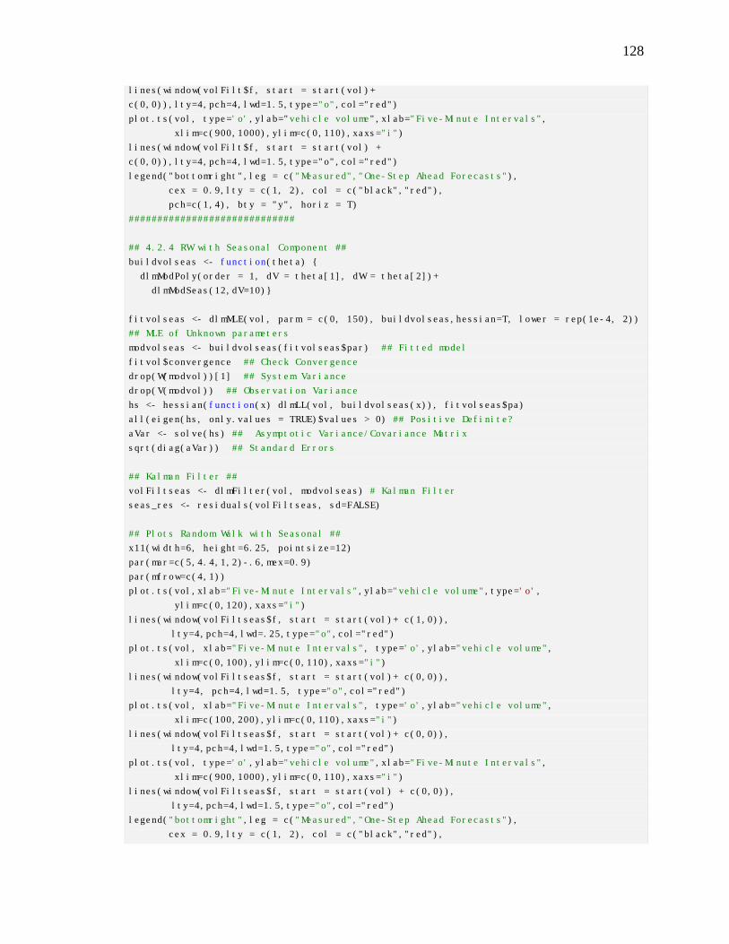
128
lines(window(volFilt$f, start = start(vol)+
c(0,0)),lty=4,pch=4,lwd=1.5,type="o",col="red")
plot.ts(vol, type='o',ylab="vehicle volume",xlab="Five-Minute Intervals",
xlim=c(900,1000),ylim=c(0,110),xaxs="i")
lines(window(volFilt$f, start = start(vol) +
c(0,0)),lty=4,pch=4,lwd=1.5,type="o",col="red")
legend("bottomright",leg = c("Measured","One-Step Ahead Forecasts"),
cex = 0.9,lty = c(1, 2), col = c("black","red"),
pch=c(1,4), bty = "y", horiz = T)
#############################
## 4.2.4 RW with Seasonal Component ##
buildvolseas <- function(theta) {
dlmModPoly(order = 1, dV = theta[1], dW = theta[2])+
dlmModSeas(12,dV=10)}
fitvolseas <- dlmMLE(vol, parm = c(0, 150), buildvolseas,hessian=T, lower = rep(1e-4, 2))
## MLE of Unknown parameters
modvolseas <- buildvolseas(fitvolseas$par) ## Fitted model
fitvol$convergence ## Check Convergence
drop(W(modvol))[1] ## System Variance
drop(V(modvol)) ## Observation Variance
hs <- hessian(function(x) dlmLL(vol, buildvolseas(x)), fitvolseas$pa)
all(eigen(hs, only.values = TRUE)$values > 0) ## Positive Definite?
aVar <- solve(hs) ## Asymptotic Variance/Covariance Matrix
sqrt(diag(aVar)) ## Standard Errors
## Kalman Filter ##
volFiltseas <- dlmFilter(vol, modvolseas) # Kalman Filter
seas_res <- residuals(volFiltseas, sd=FALSE)
## Plots Random Walk with Seasonal ##
x11(width=6, height=6.25, pointsize=12)
par(mar=c(5,4.4,1,2)-.6,mex=0.9)
par(mfrow=c(4,1))
plot.ts(vol,xlab="Five-Minute Intervals",ylab="vehicle volume",type='o',
ylim=c(0,120),xaxs="i")
lines(window(volFiltseas$f, start = start(vol)+ c(1,0)),
lty=4,pch=4,lwd=.25,type="o",col="red")
plot.ts(vol, xlab="Five-Minute Intervals", type='o',ylab="vehicle volume",
xlim=c(0,100),ylim=c(0,110),xaxs="i")
lines(window(volFiltseas$f, start = start(vol)+ c(0,0)),
lty=4, pch=4,lwd=1.5, type="o",col="red")
plot.ts(vol, xlab="Five-Minute Intervals", type='o',ylab="vehicle volume",
xlim=c(100,200),ylim=c(0,110),xaxs="i")
lines(window(volFiltseas$f, start = start(vol)+ c(0,0)),
lty=4,pch=4,lwd=1.5,type="o",col="red")
plot.ts(vol, type='o',ylab="vehicle volume",xlab="Five-Minute Intervals",
xlim=c(900,1000),ylim=c(0,110),xaxs="i")
lines(window(volFiltseas$f, start = start(vol) + c(0,0)),
lty=4,pch=4,lwd=1.5,type="o",col="red")
legend("bottomright",leg = c("Measured","One-Step Ahead Forecasts"),
cex = 0.9,lty = c(1, 2), col = c("black","red"),

129
pch=c(1,4), bty = "y", horiz = T)
#############################
## 4.2.5 Random Walk with Trig Seasonal ##
vol=ts(vol)
buildvoltrig <- function(theta) {
dlmModPoly(order = 1, dV = theta[1], dW = theta[2])+
dlmModTrig(s=12,q=6)}
fitvoltrig <- dlmMLE(vol, parm = c(0,150), buildvoltrig,hessian=T, lower = rep(1e-4, 2))
## MLE of Unknown parameters
modvoltrig <- buildvoltrig(fitvoltrig$par) ## Fitted model
fitvol$convergence ## Check Convergence
drop(W(modvol))[1] ## System Variance
drop(V(modvol)) ## Observation Variance
hs <- hessian(function(x) dlmLL(vol, buildvoltrig(x)), fitvoltrig$pa)
all(eigen(hs, only.values = TRUE)$values > 0) ## Positive Definite?
aVar <- solve(hs) ## Asymptotic Variance/Covariance Matrix
sqrt(diag(aVar)) ## Standard Errors
### Kalman Filter ###
volFilttrig <- dlmFilter(vol, modvoltrig) # Kalman Filter
trig_res <- residuals(volFiltseas, sd=FALSE)
## Plots, Random Walk with Trig Seasonal##
x11(width=6, height=6.25, pointsize=12)
par(mar=c(5,4.4,1,2)-.6,mex=0.9)
par(mfrow=c(4,1))
plot.ts(vol,xlab="Five-Minure Intervals",ylab="vehicle volume",type='o',
ylim=c(0,120),xaxs="i")
lines(window(volFilttrig$f, start = start(vol)+ c(1,0)),
lty=4,pch=4,lwd=.25,type="o",col="red")
plot.ts(vol, xlab="Five-Minute Intervals", type='o',ylab="vehicle volume",
xlim=c(0,100),ylim=c(0,110),xaxs="i")
lines(window(volFilttrig$f, start = start(vol)+ c(0,0)),
lty=4,pch=4,lwd=1.5,type="o",col="red")
plot.ts(vol, xlab="Five-Minute Intervals", type='o',ylab="vehicle volume",
xlim=c(100,200),ylim=c(0,110),xaxs="i")
lines(window(volFilttrig$f, start = start(vol)+ c(0,0)),
lty=4,pch=4,lwd=1.5,type="o",col="red")
plot.ts(vol, type='o',ylab="vehicle volume",xlab="Five-Minute Intervals",
xlim=c(900,1000),ylim=c(0,120),xaxs="i")
lines(window(volFilttrig$f, start = start(vol) + c(0,0)),
lty=4,pch=4,lwd=1.5,type="o",col="red")
legend("topright",leg = c("Measured","One-Step Ahead Forecasts"),
cex = 0.9,lty = c(1, 2), col = c("black","red"),
pch=c(1,4), bty = "y", horiz = T)
#############################

130
## Test Statistics ##
## RW Model ##
## Mean Average Deviation (MAD)
mean(c(abs(volFilt$f-vol)), na.rm=TRUE )
## Root Mean Square Error Of Prediction (RMSEP)
sqrt(1/length(vol)*sum(c(abs((volFilt$f-vol)^2)), na.rm=TRUE))
## Seasonal Based Model ##
## Mean Average Deviation (MAD)
mean(c(abs(volFiltseas$f-vol)), na.rm=TRUE )
## Root Mean Square Error Of Prediction (RMSEP)
sqrt(1/length(vol)*sum(c(abs((volFiltseas$f-vol)^2)), na.rm=TRUE))
## RW with Fourier-form Model ##
## Mean Average Deviation (MAD)
mean(c(abs(volFilttrig$f-vol)), na.rm=TRUE )
## Root Mean Square Error Of Prediction (RMSEP)
sqrt(1/length(vol)*sum(c(abs((volFilttrig$f-vol)^2)), na.rm=TRUE))

131
APPENDIX D: R CODE: TRAFFIC SPEEDS DLMS & KF
Section_4.3.R
## Code for Thesis Chapter 4.3 DLM & KF ##
## 4.3 R Model Specification and Parameter Estimation: Traffic Speeds ##
library(dlm)
library(forecast)
library(numDeriv)
Thesis_4.3 <- read.csv("C:/Users/Brian/SkyDrive/Forecasting Papers/SSwithKFfor
forecast/Kalman/Data/Thesis_4.3.csv")
spd1 <- ts(Thesis_4.3[,c(2)])
## 4.3.3 Random Walk ##
buildspd1 <- function(theta) {
dlmModPoly(order = 1, dV = theta[1], dW = theta[2])}
fitspd1 <- dlmMLE(spd1, parm = c(.2,50,75), buildspd1,hessian=T, lower = rep(1e-6))
## MLE of Unknown parameters
modspd1 <- buildspd1(fitspd1$par) ## Fitted model
fitspd1$convergence ## Check Convergence
drop(W(modspd1))[1] ## System Variance
drop(V(modspd1)) ## Observation Variance
hs <- hessian(function(x) dlmLL(spd1, buildspd1(x)), fitspd1$pa)
all(eigen(hs, only.values = TRUE)$values > 0) ## Positive Definite?
aVar <- solve(hs) ## Asymptotic Variance/Covariance Matrix
sqrt(diag(aVar)) ## Standard Errors
### Kalman Filter ###
spd1Filt <- dlmFilter(spd1, modspd1) # Kalman Filter
## 4.3.3 Plots Random Walk##
x11(width=6, height=6.25, pointsize=12)
par(mar=c(5,4.4,1,2)-.6,mex=0.9)
## 4.3.3 Plots Random Walk##
x11(width=6, height=6.25, pointsize=12)
par(mar=c(5,4.4,1,2)-.6,mex=0.9) par(mfrow=c(4,1))
plot.ts(spd1,xlab="Five-Minute Intervals",ylab="mph",type='o', ylim=c(10,90),xaxs="i")
lines(window(spd1Filt$f, start = start(spd1)+ c(1,0)),
lty=4,pch=4,lwd=.25,type="o",col="red")
plot.ts(spd1, xlab="Five-Minute Intervals", type='o',ylab="mph", xlim=c(0,100),
ylim=c(10,90),xaxs="i")
lines(window(spd1Filt$f, start = start(spd1)+c(0,0)),

132
lty=4,pch=4,lwd=1.5,type="o",col="red")
plot.ts(spd1, xlab="Five-Minute Intervals", type='o',ylab="mph",
xlim=c(100,200),ylim=c(20,90),xaxs="i")
lines(window(spd1Filt$f, start = start(spd1)+ c(0,0)),
lty=4,pch=4,lwd=1.5,type="o",col="red")
plot.ts(spd1, type='o',ylab="mph",xlab="Five-Minute Intervals",
xlim=c(600,720),ylim=c(20,90),xaxs="i")
lines(window(spd1Filt$f, start = start(spd1) + c(0,0)),
lty=4,pch=4,lwd=1.5,type="o",col="red")
legend("topright",leg = c("Measured","One-Step Ahead Forecasts"),
cex = 0.9,lty = c(1, 2), col = c("black","red"),
pch=c(1,4), bty = "y", horiz = T)
#############################
spd2 <- ts(spd1,frequency=12) ## changed to one-hour observation periods
## Speed Model w/ Seasonal Component ##
buildspdseas <- function(theta) {
dlmModPoly(order = 1, dV = theta[1], dW = theta[2])+
dlmModSeas(12)}
fitspdseas <- dlmMLE(spd2, parm = c(.1,25), buildspdseas,hessian=T,
lower = rep(1e-6)) ## MLE of Unknown parameters
modspdseas <- buildspdseas(fitspdseas$par) ## Fitted model
fitspd2$convergence ## Check Convergence
drop(W(modspdseas))[1] ## System Variance
drop(V(modspdseas)) ## Observation Variance
hs <- hessian(function(x) dlmLL(spd2, buildspdseas(x)), fitspdseas$pa)
all(eigen(hs, only.values = TRUE)$values > 0) ## Positive Definite?
aVar <- solve(hs) ## Asymptotic Variance/Covariance Matrix
sqrt(diag(aVar)) ## Standard Errors
### Kalman Filter ###
spdseasFilt <- dlmFilter(spd2, modspdseas) # Kalman Filter
## 4.3.4 Plots Random Walk with Seasonal ##
x11(width=6, height=6.25, pointsize=12)
par(mar=c(5,4.4,1,2)-.6,mex=0.9)
par(mfrow=c(4,1))
plot.ts(spd2,xlab="One-Hour Intervals",ylab="mph",type='o',
ylim=c(10,90),xaxs="i")
lines(window(spdseasFilt$f, start = start(spd2)+ c(1,0)),
lty=4,pch=4,lwd=.25,type="o",col="red")
plot.ts(spd2, xlab="One-Hour Intervals", type='o',ylab="mph",
xlim=c(0,20),ylim=c(10,90),xaxs="i")
lines(window(spdseasFilt$f, start = start(spd2)+ c(0,0)),
lty=4,pch=4,lwd=1.5,type="o",col="red")
plot.ts(spd2, xlab="One-Hour Intervals", type='o',ylab="mph",
xlim=c(20,40),ylim=c(20,90),xaxs="i")
lines(window(spdseasFilt$f, start = start(spd2)+ c(0,0)),
lty=4,pch=4,lwd=1.5,type="o",col="red")
plot.ts(spd2, type='o',ylab="mph",xlab="One-Hour Intervals",
xlim=c(40,65),ylim=c(20,90),xaxs="i")
lines(window(spdseasFilt$f, start = start(spd2) +

133
c(0,0)),lty=4,pch=4,lwd=1.5,type="o",col="red")
legend("topright",leg = c("Measured","One-Hour Intervals"),
cex = 0.9,lty = c(1, 2), col = c("black","red"),
pch=c(1,4), bty = "y", horiz = T)
#############################
## 4.3.5 Random Walk Fourier-form ##
buildspdtrig <- function(theta) {
dlmModPoly(order = 1, dV = theta[1], dW = theta[2])+
dlmModTrig(s=12,q=6)}
fitspdtrig <- dlmMLE(spd1, parm = c(.1,25), buildspdtrig,hessian=T, lower = rep(1e-6))
## MLE of Unknown parameters
modspdtrig <- buildspdtrig(fitspdtrig$par) ## Fitted model
fitspd1$convergence ## Check Convergence
drop(W(modspdtrig))[1] ## System Variance
drop(V(modspdtrig)) ## Observation Variance
hs <- hessian(function(x) dlmLL(spd1, buildspdtrig(x)), fitspdtrig$pa)
all(eigen(hs, only.values = TRUE)$values > 0) ## Positive Definite?
aVar <- solve(hs) ## Asymptotic Variance/Covariance Matrix
sqrt(diag(aVar)) ## Standard Errors
### Kalman Filter ###
spdtrigFilt <- dlmFilter(spd2, modspdtrig) # Kalman Filter
## 4.3.5 Plots Random Walk Fourier-form ##
x11(width=6, height=6.25, pointsize=12)
par(mar=c(5,4.4,1,2)-.6,mex=0.9)
par(mfrow=c(4,1))
plot.ts(spd2,xlab="One-Hour Intervals",ylab="mph",type='o',
ylim=c(10,90),xaxs="i")
lines(window(spdtrigFilt$f, start = start(spd1)+ c(1,0)),
lty=4,pch=4,lwd=.25,type="o",col="red")
plot.ts(spd2, xlab="One-Hour Intervals", type='o',ylab="mph",
xlim=c(0,20),ylim=c(10,90),xaxs="i")
lines(window(spdtrigFilt$f, start = start(spd1)+ c(0,0)),
lty=4,pch=4,lwd=1.5,type="o",col="red")
plot.ts(spd2, xlab="One-Hour Intervals", type='o',ylab="mph",
xlim=c(20,40),ylim=c(20,90),xaxs="i")
lines(window(spdtrigFilt$f, start = start(spd1)+ c(0,0)), `
lty=4,pch=4,lwd=1.5,type="o",col="red")
plot.ts(spd2, type='o',ylab="mph",xlab="One-Hour Intervals",
xlim=c(40,65),ylim=c(20,90),xaxs="i")
lines(window(spdtrigFilt$f, start = start(spd1) + c(0,0)),
lty=4,pch=4,lwd=1.5,type="o",col="red")
legend("topright",leg = c("Measured","One-Step Ahead Forecasts"),
cex = 0.9,lty = c(1, 2), col = c("black","red"),
pch=c(1,4), bty = "y", horiz = T)
#############################

134
## Test Statistics ##
## RW Model ##
## Mean Average Deviation (MAD)
mean(c(abs(spd1Filt$f-spd1)), na.rm=TRUE )
## Root Mean Square Error Of Prediction (RMSEP)
sqrt(1/length(spd1)*sum(c(abs((spd1Filt$f-spd1)^2)), na.rm=TRUE))
## Seasonal Based Model ##
## Mean Average Deviation (MAD)
mean(c(abs(spdseasFilt$f-spd2)), na.rm=TRUE )
## Root Mean Square Error Of Prediction (RMSEP)
sqrt(1/length(spd2)*sum(c(abs((spdseasFilt$f-spd2)^2)), na.rm=TRUE))
## RW with Fourier-form Model ##
## Mean Average Deviation (MAD)
mean(c(abs(spdtrigFilt$f-spd2)), na.rm=TRUE )
## Root Mean Square Error Of Prediction (RMSEP)
sqrt(1/length(spd2)*sum(c(abs((spdtrigFilt$f-spd2)^2)), na.rm=TRUE))

135
APPENDIX E: PLOTS
Figure 42. Section 1 Speed-Flow Diagram Displaying Critical Density (rhoc1)
2160, 65
0
10
20
30
40
50
60
70
80
90
0 200 400 600 800 1000 1200 1400 1600 1800 2000 2200 2400
Spee
d (m
ph)
Flow (veh/hr)
Lane1 Lane2 Lane3 Lane4

136
Figure 43. Section 2 Speed-Flow Diagram Displaying Critical Density (rhoc2)
2172, 53
0
10
20
30
40
50
60
70
80
90
0 200 400 600 800 1000 1200 1400 1600 1800 2000 2200 2400
Spee
d (m
ph)
Flow (veh/hr)
Lane1 Lane2 Lane3 Lane4