The Endogenous Grid Method for Discrete-ContinuousDynamic Choice Models with (or without) Taste Shocks †

Fedor IskhakovAustralian National University and CEPAR UNSW

Thomas H. JørgensenUniversity of Copenhagen

John RustGeorgetown University

Bertel SchjerningUniversity of Copenhagen

September 2016

Abstract: We present a fast and accurate computational method for solving and estimating a class ofdynamic programming models with discrete and continuous choice variables. The solution method wedevelop for structural estimation extends the endogenous gridpoint method (EGM) to discrete-continuous(DC) problems. Discrete choices can lead to kinks in the value functions and discontinuities in the optimalpolicy rules, greatly complicating the solution of the model. We show how these problems are amelioratedin the presence of additive choice-specific IID extreme value taste shocks which are typically interpretedas “unobserved state variables” in structural econometric applications, or serve as “random noise” tosmooth out kinks in the value functions in numerical applications. We present Monte Carlo experimentsthat demonstrate the reliability and efficiency of the DC-EGM and the associated Maximum Likelihoodestimator for structural estimation of a life cycle model of consumption with discrete retirement decisions.

Keywords: Lifecycle model, discrete and continuous choice, retirement choice, endogenous gridpointmethod, nested fixed point algorithm, extreme value taste shocks, smoothed max function, structuralestimation.

JEL classification: C13, C63, D91

† We acknowledge helpful comments from Chris Carroll and many other people, participants at seminars at UNSW,

University og Copenhagen, the 2012 conferences of the Society of Economic Dynamics, the Society for Computa-

tional Economics, the Initiative for Computational Economics at Zurich (ZICE 2014, 2015). This paper is part of the

IRUC research project financed by the Danish Council for Strategic Research (DSF). Iskhakov, Rust and Schjerning

gratefully acknowledge this support. Iskhakov gratefully acknowledges the financial support from the Australian

Research Council Centre of Excellence in Population Ageing Research (project number CE110001029) and Michael

P. Keane’s Australian Research Council Laureate Fellowship (project number FL110100247). Jørgensen gratefully

acknowledges financial support from the Danish Council for Independent Research in Social Sciences (FSE, grant

no. 4091-00040). Correspondence address: Research School of Economics, ANU College of Business and Eco-

nomics, 1018 HWArndt building, The Australian National University, Canberra, ACT 0200 phone: (+61)261256193,

email: fedor.iskhakov@anu.edu.au

1 Introduction

This paper develops a fast new solution algorithm for structural estimation of dynamic program-

ming models with discrete and continuous choices. The algorithm we propose extends the Endoge-

nous Grid Method (EGM) by Carroll (2006) to discrete-continuous (DC) models. We refer to it as

the DC-EGM algorithm. We embed the DC-EGM algorithm in the inner loop of the nested fixed

point (NFXP) algorithm (Rust, 1987), and show that the resulting maximum likelihood estimator

produces accurate estimates of the structural parameters at low computational cost.

A classic example of a DC model is a life cycle model with discrete retirement and continuous

consumption decisions. While there is a well developed literature on solution and estimation of

dynamic discrete choice models, and a separate literature on estimation of life cycle models without

discrete choices, there has been far less work on solution and estimation of DC models.1

There is good reason why DC models are much less commonly seen in the literature: they

are substantially harder to solve. The value functions of models with only continuous choices are

typically concave and the optimal policy function can be found from the Euler equation. EGM

avoids the need to numerically solve the nonlinear Euler equation for the optimal continuous choice

at each grid point in the state space. Instead, EGM specifies an exogenous grid over an endogenous

quantity, e.g. savings, to analytically calculate the optimal policy rule, e.g., consumption, and

endogenously determine the pre-decision state, e.g., beginning-of-period resources.2 DC-EGM

retains the main desirable properties of EGM, namely it avoids the bulk of root-finding operations

and handles borrowing constraints in an efficient manner.

Dynamic programs that have only discrete choices are substantially easier to solve, since the

optimal decision rule is simply the alternative with highest choice-specific value. However, solving

dynamic programming problems that combine continuous and discrete choices is substantially

more complicated, since discrete choices introduce kinks and non-concave regions in the value

1There are relatively few examples of structural estimation or numerical solution of DC models. Some promi-nent examples include the model of optimal non-durable consumption and housing purchases (Carroll and Dunn,1997), optimal saving and retirement (French and Jones, 2011), and optimal saving, labor supply and fertility(Adda, Dustmann and Stevens, forthcoming).

2The EGM is in fact a specific application of what is referred to as “controlling the post-decision state”in operations research and engineering (Bertsekas, Lee, van Roy and Tsitsiklis, 1997). Carroll (2006) introducedthe idea in economics by developing the EGM algorithm with the application to the buffer-stock precaution-ary savings model. Since then the idea became widespread in economics. Further generalizations of EGM in-clude Barillas and Fernandez-Villaverde (2007); Hintermaier and Koeniger (2010); Ludwig and Schon (2013); Fella(2014); Iskhakov (2015). Jørgensen (2013) compares the performance of EGM to Mathematical Programming withEquilibrium Constraints (MPEC).

1

function that lead to discontinuities in the policy function of the continuous choice (consumption).

This can lead to situations where the Euler equation has multiple solutions for consumption, and

hence it is only a necessary rather than a sufficient condition for the optimal consumption rule

(Clausen and Strub, 2013). This inherent feature of DC problems complicates any method one

might consider for solving DC models.

We illustrate how DC-EGM can deal with these inherent complications using a life cycle model

with a continuous consumption and binary retirement choice with and without taste shocks. Our

example is a simple extension of the classic life cycle model of Phelps (1962) where, in the absence

of a retirement decision, the optimal consumption rule could hardly be any simpler — a linear

function of resources. However, once the discrete retirement decision is added to the Phelp’s

problem — in our case allowing a worker with logarithmic utility to also make a binary irreversible

retirement decision — the consumption function becomes unexpectedly complex, with multiple

discontinuities in the optimal consumption rule. We derive an analytic solution for this model,

use it to demonstrate the accuracy of the solution obtained numerically by DC-EGM, and then

investigate the performance of the Rust’s NFXP type nested estimator based on the DC-EGM

solution algorithm to estimate the structural parameters of this model.

Fella (2014) showed how EGM could be adapted to solve non-concave problems, including mod-

els with discrete and continuous choices. In this paper we focus on discrete choices and show that

introducing IID Extreme Value Type I choice-specific taste shocks not only facilitates maximum

likelihood estimation, but also allows to smooth out some of the kinks in the value functions and

thus simplify the numerical solution of DC models. This approach results in multinomial logit for-

mulas for the conditional choice probabilities for the discrete choices and a closed form expression

for the expectation of the value function with respect to these taste shocks.3

In econometric applications continuously distributed taste shocks are essential for generating

predictions from dynamic programming models that are statistically non-degenerate. Such pre-

dictions assign a positive (however small) choice probability to every alternative, and therefore

preclude zero likelihood observations. These shocks are interpreted as unobserved state variables,

i.e. idiosyncratic shocks observed by agents but not by the econometrician. However, in numerical

3In principle, the Extreme Value assumption could be relaxed to allow for other distributions at the cost ofnumerical approximation of choice probabilities and the conditional expectation of the value function. For example,Bound, Stinebrickner and Waidmann (2010), assume that the discrete choice specific taste shocks are Normal ratherthan Extreme Value. Yet, we follow the long tradition of discrete choice modeling dating back to (McFadden, 1973)and (Rust, 1987).

2

or theoretical applications taste shocks can serve as a smoothing device (homotopy perturbation)

that facilitates the numerical solution of more advanced DC models that may have excessively

many kinks and discontinuities, for example caused by a large number of discrete choices.

The inclusion of Extreme Value Type I taste shocks have a long history in discrete choice

modeling dating back to the seminal work by McFadden (1973). This assumption is typically

invoked in microeconometric analyses of dynamic discrete choice models where numerical per-

formance boosted by closed form choice probabilities is particularly important, see for example

Rust (1994) and the recent survey by Aguirregabiria and Mira (2010). Some recent studies of DC

models with Extreme Value taste shocks include Casanova (2010); Ejrnæs and Jørgensen (2015);

Iskhakov and Keane (2016); Oswald (2016) and Adda, Dustmann and Stevens (forthcoming).

At first glance, the addition of stochastic shocks would appear to make the problem harder to

solve, since both the optimal discrete and continuous decision rules will necessarily be functions

of these stochastic shocks. However, we show that a variety of stochastic variables in DC models

smooth out many of the kinks in the value functions and the discontinuities in the optimal con-

sumption rules. In the absence of smoothing, we show that every kink induced by the comparison

of the discrete choice specific value functions in any period t propagates backwards in time to

all previous periods as a manifestation of the decision maker’s anticipation of the future discrete

action. The resulting accumulation of kinks during backward induction presents the most signif-

icant challenge for the numerical solution of DC models. In presence of taste shocks the decision

maker can only anticipate a particular future discrete action to be more or less probable, and

thus the primary reason for the accumulation of kinks disappears. Yet, the combination of taste

shocks and the stochastic variables in the model is perhaps the most powerful device to prevent

the propagation and accumulation of kinks.4

In the case when the Extreme Value taste shocks are used as a logit smoothing device of an

underlying deterministic model of interest, we show that the latter problem can be approximated

by the smoothed model to any desirable degree of precision. The scale parameter σ ≥ 0 of the

corresponding Extreme Value distribution then serves as a homotopy or smoothing parameter.

When σ is sufficiently large, the non-concave regions near the kinks in the non-smoothed value

function disappear and the value functions become globally concave. But even small values of

4Contrary to the macro literature that uses stochastic elements such as employment lotteries (Rogerson, 1988;Prescott, 2005; Ljungqvist and Sargent, 2005) to smooth out non-convexities, the taste shock we introduce in DCmodels in general do not fully convexify the problem.

3

σ smooth out many of the kinks in the value functions and suppress their accumulation in the

process of backward induction as noted above. An additional benefit of the taste shocks is that

standard integration methods, such as quadrature rules, apply when the expected value function

is a smooth function.

We run a series of Monte Carlo simulations to investigate the performance of DC-EGM for

structural estimation of the life cycle model with the discrete retirement decision. We find that a

maximum likelihood estimator that nests the DC-EGM algorithm performs well. It quickly pro-

duces accurate estimates of the structural parameters of the model even when fairly coarse grids

over wealth are used. We find the cost of “oversmoothing” to be negligible in the sense that the

parameter estimates of a perturbed model with stochastic taste shocks are estimated very accu-

rately even if the true model does not have taste shocks. Thus, even in the case where the addition

of taste shocks results in a misspecification of the model, the presence of these shocks improves the

accuracy of the solution and reduces computation time without increasing the approximation bias

significantly. Even when very few grid points are used to solve the model, we find that smoothing

the problem improves the root mean square error (RMSE). Particularly, with an appropriate de-

gree of smoothing (σ), we can reduce the number of gridpoints by an order of magnitude without

much increase in the RMSE of the parameter estimates.

DC-EGM is applicable to many fields of economics and has been implemented in several recent

empirical applications. Ameriks, Briggs, Caplin, Shapiro and Tonetti (2015) study how the need

for long term care and bequest motive interact with government-provided support to shape the

wealth profile of the elderly. They use an endogenous grid method similar to DC-EGM to solve

and estimate the corresponding non-concave model. Iskhakov and Keane (2016) employ DC-EGM

to estimate a life-cycle model of discrete labor supply, human capital accumulation and savings

for the Australian population. They use the model to evaluate Australia’s defined contribution

pension scheme with means-tested minimal pension, and quantify the effects of anticipated and

unanticipated policy changes. Yao, Fagereng and Natvik (2015) use DC-EGM to analyze how

housing and mortgage debt affects consumer’s marginal propensity to consume. They estimate

a model in which households hold debt, financial assets and illiquid housing and find that a

substantial fraction of households are likely to behave in a “hand-to-mouth” fashion despite having

significant wealth holdings. Druedahl and Jørgensen (2015) employ a modified version of DC-EGM

to analyze the credit card debt puzzle. They solve a model of optimal consumption and debt

4

holdings and show how, for some parameterizations of the model, a large group of consumers find

it optimal to simultaneously hold positive gross debt and positive gross assets even though the

interest rate on the debt is much higher than the rate on the assets. Ejrnæs and Jørgensen (2015)

use DC-EGM to estimate a model of optimal consumption and saving with a fertility choice to

analyze the saving behavior around intended and unintended childbirths. They model the fertility

process as a discrete choice over effort to conceive a child subject to a biological fecundity constraint

and allow for the possibility of unintended child births through imperfect contraceptive control.

In the next section we present a simple extension of the life cycle model of consumption and

savings with logarithmic utility studied by Phelps (1962) where we allow for a discrete retirement

decision. We derive a closed-form solution to this problem, and discuss its properties. Using

this simple model we demonstrate the accuracy of the deterministic version of DC-EGM. We

then introduce extreme value taste shocks and show how the implied smoothing affects the value

functions and the optimal policy rules. In particular, we show that the error introduced by “extreme

value smoothing” is uniformly bounded, and prove that the solution of the smoothed DP problem

with taste shocks converges to the solution to the DP problem without taste shocks as scale of the

shocks approaches zero. Section 3 presents the full DC-EGM algorithm. In section 4 we show how

it is incorporated in the Nested Fixed Point algorithm for maximum likelihood estimation of the

structural parameters in the retirement model. We present the results of a series of Monte Carlo

experiments in which we explore the performance of the estimator in a variety of settings. We

conclude with a short discussion of the range of models that DC-EGM is applicable to and discuss

some open issues with this method.

2 An Illustrative Problem: Consumption and Retirement

This section extends the classic life-cycle consumption/savings model of Phelps (1962) to allow

for a binary retirement decision. We derive an analytic solution to the simple life cycle problem

with logarithmic utility that serves both to illustrate the complexity caused by the addition of

a discrete retirement choice and how DC-EGM can be applied. While we focus on this simple

illustrative example for expositional clarity, DC-EGM can be applied in a much more general class

of problems that we discuss in the conclusion - including the extended version of the retirement

model that we use in the Monte Carlo exercise. While we initially illustrate the complexity of the

5

solution without any stochastic elements, we include both taste and income shocks in the simple

model and discuss how these additional elements actually simplify the solution of the model using

DC-EGM.

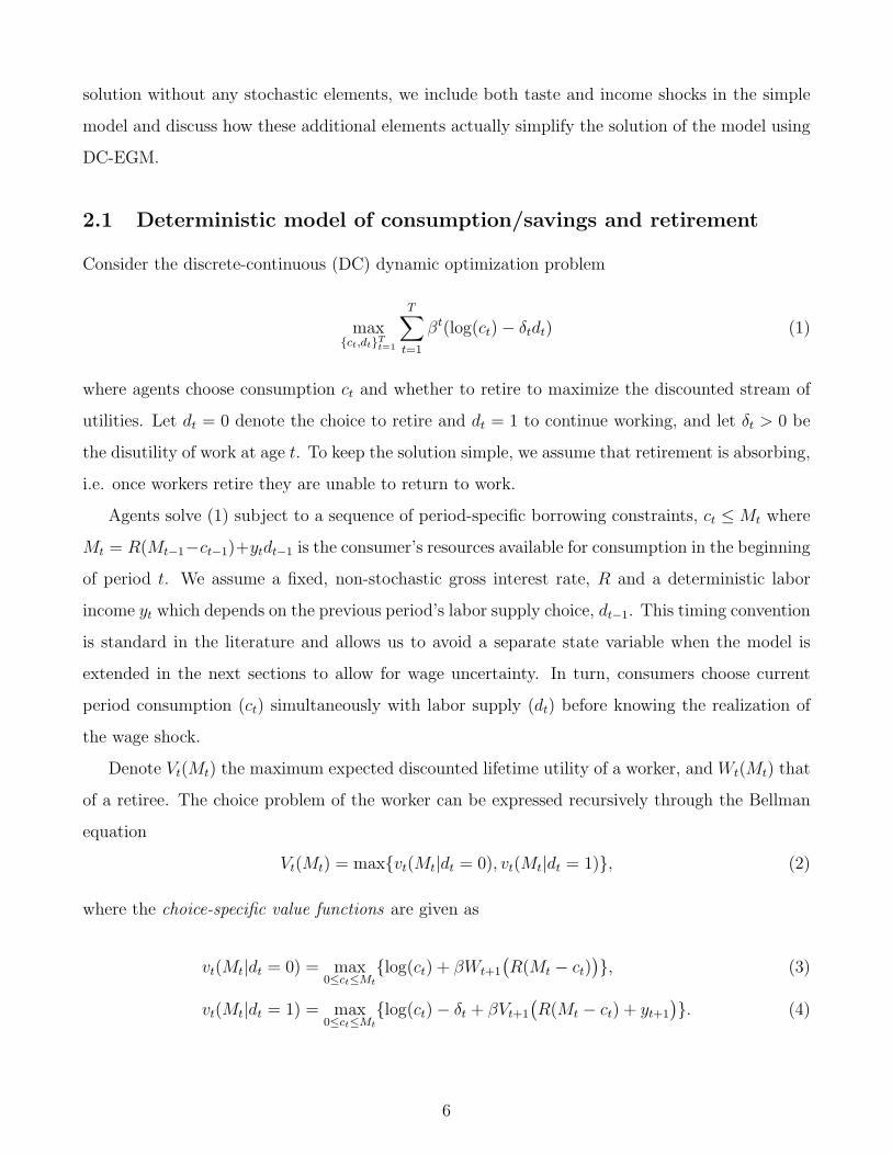
2.1 Deterministic model of consumption/savings and retirement

Consider the discrete-continuous (DC) dynamic optimization problem

max{ct,dt}Tt=1

T∑t=1

βt(log(ct)− δtdt) (1)

where agents choose consumption ct and whether to retire to maximize the discounted stream of

utilities. Let dt = 0 denote the choice to retire and dt = 1 to continue working, and let δt > 0 be

the disutility of work at age t. To keep the solution simple, we assume that retirement is absorbing,

i.e. once workers retire they are unable to return to work.

Agents solve (1) subject to a sequence of period-specific borrowing constraints, ct ≤ Mt where

Mt = R(Mt−1−ct−1)+ytdt−1 is the consumer’s resources available for consumption in the beginning

of period t. We assume a fixed, non-stochastic gross interest rate, R and a deterministic labor

income yt which depends on the previous period’s labor supply choice, dt−1. This timing convention

is standard in the literature and allows us to avoid a separate state variable when the model is

extended in the next sections to allow for wage uncertainty. In turn, consumers choose current

period consumption (ct) simultaneously with labor supply (dt) before knowing the realization of

the wage shock.

Denote Vt(Mt) the maximum expected discounted lifetime utility of a worker, and Wt(Mt) that

of a retiree. The choice problem of the worker can be expressed recursively through the Bellman

equation

Vt(Mt) = max{vt(Mt|dt = 0), vt(Mt|dt = 1)}, (2)

where the choice-specific value functions are given as

vt(Mt|dt = 0) = max0≤ct≤Mt

{log(ct) + βWt+1

(R(Mt − ct)

)}, (3)

vt(Mt|dt = 1) = max0≤ct≤Mt

{log(ct)− δt + βVt+1

(R(Mt − ct) + yt+1

)}. (4)

6

The choice problem of the retiree is given by the Bellman equation

Wt(Mt) = max0≤ct≤Mt

{log(ct) + βWt+1

(R(Mt − ct)

)}. (5)

It follows from (3) and (5) that vt(Mt|dt = 0) = Wt(Mt). The value function Wt(Mt) is given

by Phelps (1962, p. 742) who solves the corresponding optimal consumption problem. In the

following we therefore only focus on deriving formulas for vt(Mt|dt = 1) and finding optimal

consumption rules ct(Mt|dt = 0) and ct(Mt|dt = 1) for a worker who chooses to retire and to

continue working, respectively. It follows that the optimal consumption rule for the retiree is

identical to ct(Mt|dt = 0).

Note that even if vt(Mt, 0) and vt(Mt, 1) are concave functions of Mt, because Vt(Mt) is the

maximum of the two, it is generally not concave (Clausen and Strub, 2013). It is not hard to show

that Vt will generally have a kink point at the value of resources where the two choice-specific value

functions cross (M t), i.e. where vt(M t, 1) = vt(M t, 0). We refer to these points as primary kinks.

This kink point at M t is also the optimal retirement threshold — the optimal decision for a

worker with resources Mt ≤ M t is to keep working (not to retire) and to use the consumption rule

ct(Mt|dt = 1), whereas the optimal decision for a worker whose wealth exceeds M t is to retire and

to consume ct(Mt|dt = 0). The worker is indifferent between retiring and working at the primary

kinks (M = M t) where the value function is generally non-differentiable. However the left and right

hand derivatives do exist and we have V −t (M t) < V +

t (M t). Through the first order conditions,

the discontinuity in the derivative of Vt(M) at M t translates into a discontinuity in the optimal

consumption function in the previous period t−1. In the same time, because the Bellman equation

expresses Vt−1(M) as a function of Vt(M), the kink point in the latter results in a kink in Vt−1(M).

In effect, the primary kinks propagate back in time and manifest themselves as discontinuities in

the policy functions and additional kinks in the value function. These kinks do not correspond to

the points of indifference between the discrete alternatives, but instead appear as reverberations

of the primary kinks at the retirement thresholds the consumer expects to encounter in the future.

We refer to these as secondary kinks.

Let cT−τ (M) denote the optimal consumption function of the workers in period t = T − τ ,

i.e. τ periods before the end of the life cycle. Theorem 1 illustrates how complex the solution

to Phelps’ model becomes once we make the simple extension of allowing a discrete, irreversible

retirement choice.

7

Theorem 1 (Analytical solution to the retirement problem). Assume that income and disutility

of work are time-invariant and the discount factor β and the disutility of work δ are not too large,

i.e.

βR ≤ 1 and δ < (1 + β) log(1 + β). (6)

Then τ ∈ {1, . . . , T} the optimal consumption rule in the workers’ problem (2)-(4) is given by

cT−τ (M) =

M if M ≤ y/Rβ,

[M + y/R]/(1 + β) if y/Rβ ≤ M ≤ Ml1T−τ ,

[M + y(1/R + 1/R2)]/(1 + β + β2) if Ml1T−τ ≤ M ≤ M

l2T−τ ,

· · · · · ·[M + y

(∑τ−1i=1 R−i

)] (∑τ−1i=0 βi

)−1if M

lτ−2

T−τ ≤ M ≤ Mlτ−1

T−τ ,

[M + y (∑τ

i=1 R−i)] (

∑τi=0 β

i)−1

if Mlτ−1

T−τ ≤ M < Mrτ−1

T−τ ,[M + y

(∑τ−1i=1 R−i

)](∑τ

i=0 βi)−1

if Mrτ−1

T−τ ≤ M < Mrτ−2

T−τ ,

· · · · · ·

[M + y(1/R + 1/R2)] (∑τ

i=0 βi)−1

if Mr2T−τ ≤ M < M

r1T−τ ,

[M + y/R] (∑τ

i=0 βi)−1

if Mr1T−τ ≤ M < MT−τ ,

M (∑τ

i=0 βi)−1

if M ≥ MT−τ .

(7)

The segment boundaries are totally ordered with

y/Rβ < Ml1T−τ < · · · < M

lτ−1

T−τ < Mrτ−1

T−τ < · · · < Mr1T−τ < MT−τ , (8)

and the right-most threshold MT−τ given by

MT−τ =(y/R)e−K

1− e−K, where K = δ

(τ∑

i=0

βi

)−1

, (9)

defines the smallest level of wealth sufficient to induce the consumer to retire at age t = T − τ .

The proof of Theorem 1 is given in Appendix C. Note that the assumptions on the parameters β,

δ and R are needed to ensure the ordering of the bounderies (8). Modified versions of Theorem 1

hold under weaker conditions, including a version where income and the disutility of work are

age-dependent. However, depending on the paths of income and disutility of work some of the

intermediate thresholds in Theorem 1 may not exist, or may be equal to each other.

8

It follows that the optimal consumption rule (7) is piece-wise linear inM , and in period t = T−τ

consists of 2τ + 1 segments. The first segment where M < y/Rβ is the credit constrained region.

The next τ − 1 segments are connected and bounded by the τ − 1 kink points MljT−τ which

represents the largest levels of wealth for which the consumer is not liquidity constrained at ages

T − τ, T − τ + 1, . . . , T − τ + j − 1, but will be liquidity constrained at age T − τ + j under

the optimal consumption and retirement policy. The remaining segments relate to the retirement

choice, namely MrjT−τ , j = 1, . . . , τ − 1 represent the largest level of saving for which it is optimal

to retire at age T − τ + j but not at any earlier age T − τ, T − τ + 1, . . . , T − τ + j − 1. The

optimal consumption function is discontinuous at points MrjT−τ , and including the discontinuity at

the retirement threshold MT−τ makes altogether τ downward jumps in period T − τ .

Using Theorem 1 it is not hard to show that the value function VT−τ (M) is piecewise logarithmic

with the same kink points, and can be written as

VT−τ (M) = BT−τ log(cT−τ (M)) + CT−τ (10)

for constants (BT−τ , CT−τ ) that depend on the regionM falls in. For each τ ≥ 1, the value function

has one primary kink at the optimal retirement threshold M = MT−τ , τ − 1 secondary kinks at

MrjT−τ , j = 1, . . . , τ − 1, and τ kinks related to current period and future liquidity constraints at

M = y/Rβ and MljT−τ , j = 1, . . . , τ − 1. If Rβ = 1 the liquidity-related kink points collapse to a

single point M = y/Rβ = y = Ml1T−τ = · · · = M

lτ−1

T−τ .

Figure 1 displays the optimal consumption function (7) and compares it to the numerical

solution produced by DC-EGM described below in Section 3, as well as the numerical solution

produced by a naive brute force implementation of VFI. With a sufficient number of grid points,

DC-EGM is able to accurately locate all the discontinuities of the analytical consumption rules

(MrjT−τ ) and the boundary of the credit constrained region y/Rβ. Yet, because the kinks points

MljT−τ are not located precisely, the right panel of Figure 1 shows small relative errors on the order

of 10−4 in the intervals (y/Rβ,Mτ−1

T−τ ) in each period T − τ . Overall, the numerical solution by

DC-EGM replicates the analytical solution remarkably well.5

5With 2000 points on the endogenous grid over wealth it took our Matlab/C implementation around 0.17 sec-

onds on a Lenovo ThinkPad laptop with Intel R⃝ CoreTM

i7-4600M CPU @ 2.10 GHz and 8GB RAM to generatethe numerical solution by DC-EGM. This is about 20 times faster than value function iterations (VFI) whichwe implemented in Matlab with 500 fixed grid points over wealth. The discretization of consumption is a bruteforce approach to ensure that global optimum is found. We used 400 equally spaced guesses for each level ofwealth. The fact that EGM offers the speedup of one to two orders of magnitude relative to VFI is a well estab-

9

Figure 1: Optimal Consumption Functions.

(a) Analytical Solution

0 50 100 150 200 250 300 350 400

Resources, M

0

5

10

15

20

25

30

35

40

Con

sum

ptio

n, c

t=1

t=10

t=18

(b) Relative Error of DC-EGM solution

0 50 100 150 200 250 300 350 400

Resources, M

-2.5

-2

-1.5

-1

-0.5

0

0.5

Rel

ativ

e er

ror,

×10

4

(c) Off the shelf VFI solution

0 50 100 150 200 250 300 350 400

Resources, M

0

5

10

15

20

25

30

35

40

Con

sum

ptio

n, c

t=1

t=10

t=18

(d) Relative Error of VFI solution

0 50 100 150 200 250 300 350 400

Resources, M

-2000

-1500

-1000

-500

0

500

1000

1500

Rel

ativ

e er

ror,

×10

4 (

vfi)

Notes: The plots show optimal consumption rules of the worker in the consumption-savings model with R = 1,

β = 0.98, y = 20, and T = 20. Panel (a) illustrates the analytical solution (which is indistinguishable from the

the numerical solution produced by DC-EGM), panel (b) illustrates the numerical error from the solution found by

DC-EGM. Panel (c) shows the numerical solution found by value function iterations (VFI), and panel (d) shows the

associated numerical errors. Both the VFI and DC-EGM solutions were generated using 2000 points in the M -grid.

For VFI grid points are equally spaced, the maximum level in the wealth is 600, and 10,000 equally spaced between

zero and M(t) points of consumption are used to solve the maximization problem in the Bellman equation.

10

Figure 2: Discontinuous Consumption Function and Smooth Consumption Paths

(a) Consumption Function

0 50 100 150 200 250 300 350 400

Resources, M

0

5

10

15

20

25

30

35

40

Con

sum

ptio

n, c

t=1

t=10

t=18

(b) Simulated Consumption Paths

0 2 4 6 8 10 12 14 16 18 20

Timeperiod, t

19.5

19.6

19.7

19.8

19.9

20

20.1

20.2

20.3

20.4

20.5

DC-EGM, A0=1

DC-EGM, A0=50

DC-EGM, A0=100

DC-EGM, A0=150

Retirement year

Notes: The plots show optimal consumption functions of the worker in the consumption-savings model with with

T = 20, dt = 1, y = 20, β = .98, and R = 1/β = 1.02. The left panel illustrates the solution for t = 1, 10, 18, while

the right panel presents consumption paths simulated over the whole life cycle for several initial levels of wealth.

The model was solved by the DC-EGM algorithm.

Panels (c)-(d) of Figure 1 show the solution produced by a traditional value function iterations

(VFI) method with the same number of grid points over wealth and optimal consumption levels

found by a fine grid search method. This implementation of VFI could admittedly be thought

of as too simplistic, with possible improvements in how the grid points are located and spaced,

which computational methods are employed to search for optimal consumption in each grid point,

etc. Yet, the point we wish to make is that a standard “off the shelf” version of the VFI method

may have serious difficulties when solving DC problems due to its failure to adequately capture the

secondary kinks in the value function that get “papered over” via naive application of the standard

method of linear interpolation of the value functions. The bottom panels of Figure 1 shows that

the VFI solution results in significant approximation errors and is unable to fully capture the

numerous discontinuities in the consumption function.

Figure 2 plots the optimal consumption functions and simulated consumption paths under the

same assumptions as in Figure 1 except in this case we set R = 1/β = 1.02. The theoretical

lished finding in the literature, see e.g. Barillas and Fernandez-Villaverde (2007); Jørgensen (2013); Fella (2014);Ameriks, Briggs, Caplin, Shapiro and Tonetti (2015).

11

prediction is that, with Rβ = 1, simulated consumption paths should be flat, yet the consumption

functions shown in the left panel displays numerous discontinuities that accumulate backwards from

the final period T = 20. Beyond the important economic message that discontinuous consumption

functions are not incompatible with consumption smoothing, this also illustrates the remarkable

precision of the DC-EGM algorithm. In fact, when we simulate consumption trajectories implied

by this incredibly complex solution found numerically, the simulated consumption profiles are still

perfectly flat.

Before we describe in detail how DC-EGM works, we now illustrate how the incorporation

of various types of uncertainty, including Extreme value taste shocks, renders the accumulation

of kinks in the value function and discontinuities in the consumption function considerably less

severe.

2.2 Adding Taste Shocks and Income Uncertainty

Now consider an extension of the model presented above where the consumer faces income uncer-

tainty and where choices are affected by choice-specific taste shocks. More specifically, assume that

income when working is yt = yηt, where ηt is log-normally distributed multiplicative idiosyncratic

income shock, log ηt ∼ N (−σ2η/2, σ

2η).

6

The additively separable choice-specific random taste shocks, σεεt(dt), are i.i.d. Extreme Value

type I distributed with scale parameter σε. In this formulation, the extreme value taste shock

enters as a structural part of the problem. If the true model does not have taste shocks, σε can be

interpreted as a (logit) smoothing parameter, see Theorem 2 below.

The solution of the retiree’s problem remains the same, and we focus on the worker’s problem.

The Bellman equation (2) has to be rewritten to include the taste shocks,

Vt(Mt, εt) = max{vt(Mt|dt = 0) + σεεt(0), vt(Mt|dt = 1) + σεεt(1)}, (11)

where the value function conditional on the choice to retire vt(Mt|dt = 0) is given by (3). However,

the value function conditional on the choice to remain working, vt(Mt|dt = 1), is modified to

6As mentioned above, we follow the literature in the assumption that idiosyncratic income shocks are realizedafter the labor supply choice is made, which is equivalent to allowing income to be dependent on a lagged choice oflabor supply.

12

account for the taste and income shocks in the following period,

vt(Mt|dt = 1) = max0≤ct≤Mt

{log(ct)− 1 + β

∫EV σε

t+1(R(Mt − ct) + yηt+1)f(dηt+1)

}. (12)

Because the taste shocks are independent Extreme Value distributed random variables, the ex-

pected value function, EV σεt+1, is given by the well-known logsum formula (McFadden, 1973)

EV σεt+1(Mt+1) = E

[max

{vt+1(Mt+1|dt+1 = 0) + σεε(0), vt+1(Mt+1|dt+1 = 1) + σεε(1)

}]= σε log

{exp

[vt+1(Mt+1|dt+1 = 0)

σε

]+ exp

[vt+1(Mt+1|dt+1 = 1)

σε

]}. (13)

The immediate effect of introducing extreme value taste shocks is the complete elimination of

the primary kinks due to the smoothing of the logit formula: the expected value function in (13)

is a smooth function of Mt around the point where vt(Mt|dt = 1) = vt(Mt|dt = 0). When σε

is sufficiently large the value function vt(Mt|dt = 1) eventually becomes globally concave.7 Even

when σε is not large enough to “concavify” the value function completely, by smoothing out the

primary kink in period t it still helps to eliminate many of the secondary kinks in the time periods

prior to t.

Figure 3 shows the choice specific consumption function ct(Mt|dt = 1) for a worker

(conditional on the choice to continue working) for different values of smoothing parameter

σε ∈ {0, 0.01, 0.05, 0.10, 0.15}. The left panel plots the optimal consumption in the absence of

income uncertainty (ση = 0) while income uncertainty (ση =√0.005) is added in the right panel.

The plots are drawn for the period T − 5, corresponding to 4 discontinuities of the choice specific

policy function in line with Theorem 1, without the discontinuity at the retirement thresholdMT−5

in the deterministic model.

7To see this, note that as the variance of the taste shocks increases, the choice-specific value functions aredominated by the noise and the differences between the alternatives become relatively less important. In turn, thechoice-specific value functions become similar, and limσε↓∞ EV σε

t (Mt)/σε = log(2). It follows from (11) then thatthe value function vt(Mt|dt = 1) inherits its globally concave shape from the utility function.

13

Figure 3: Optimal Consumption Rules for Agent Working Today (dt−1 = 1).

(a) Without income uncertainty, ση = 0

20 40 60 80 100 12015

16

17

18

19

20

21

22

23

24

25

Resources, m

Con

sum

ptio

n, c

σε = 0

σε = 0.01

σε = 0.05

σε = 0.10

σε = 0.15

(b) With income uncertainty, ση =√.005

20 40 60 80 100 12015

16

17

18

19

20

21

22

23

24

25

Resources, m

Con

sum

ptio

n, c

σε = 0

σε = 0.01

σε = 0.05

σε = 0.10

σε = 0.15

Notes: The plots show optimal consumption rules of the worker who decides to continue working in the consumption-

savings model with retirement in period t = T − 5 for a set of taste shock scales σε in the absence of income

uncertainty, ση = 0, (left panel) and in presence of income uncertainty, ση =√.005, (right panel). The rest of the

model parameters are R = 1, β = 0.98, y = 20.

Figure 4: Artificial Discontinuities in Consumption Functions, σ2η = 0.01, t = T − 3.

(a) σε = 0

28 29 30 31 32 33 3418

19

20

21

22

23

24

Resources, m

Con

sum

ptio

n

VFI, 10 discrete pointsDC−EGM, 10 discrete pointsVFI, 200 discrete pointsDC−EGM, 200 discrete points

(b) σε = 0.05

28 29 30 31 32 33 3418

19

20

21

22

23

24

Resources, m

Con

sum

ptio

n

VFI, 10 discrete pointsDC−EGM, 10 discrete pointsVFI, 200 discrete pointsDC−EGM, 200 discrete points

Notes: Figure 4 illustrates how the number of discrete points used to approximate expectations regarding future

income affects the consumption functions from value function iteration (VFI) and DC-EGM. Panel (a) illustrates

how using few (10) discrete equiprobable points to approximate expectations produce severe approximation error

when there is no taste shocks. Panel (b) illustrates how moderate smoothing (σε = .05) significantly reduces this

approximation error.

14

It is evident that taste shocks of larger scale (σε ≥ 0.05) manage to smooth the function

completely — eliminating all four discontinuities, and thus, eliminating the non-concavity of the

value function in period T−4. Yet, for σε = 0.01 only the last (rightmost) discontinuity is obviously

smoothed out. Thus, even though full “concavification” is not achieved, the presence of extreme

value taste shocks makes the consumption function continuous by smoothing out the secondary

kinks in the value function.

When the model has other stochastic elements such as wage shocks or random market returns,

the accumulation of secondary kinks may be less pronounced due to the additional smoothing. Yet,

in the absence of taste shocks, the primary kinks cannot be avoided even if all secondary kinks

are eliminated by a sufficiently high degree of uncertainty in the model. It is in this setup which

also appears to be mostly used in practical applications, where the introduction of the Extreme

Value distributed taste shocks is especially beneficial. The taste shocks and other structural shocks

together contribute to the reduction of the number of secondary kinks and to the alleviation of

the issue of their multiplication and accumulation. It is clear from the right panel of Figure 3 that

the non-concavity of the value function can be eliminated with a smaller taste shock (σε = 0.01)

when additional smoothing through uncertainty is present in the model.

An additional benefit of the inclusion of taste shocks is that numerical integration over the

stochastic elements of the model has to be performed on a smooth function EV σεt (Mt) instead

of the kinked value function Vt(Mt). Standard procedures like Gaussian quadrature are readily

applicable. When σε = 0, performing standard numerical integration typically results in spurious

discontinuities as shown in the left panel of Figure 4. This is due to the integrand not being a

smooth function, see Appendix B for a detailed discussion. The right panel of Figure 4 illustrates

how moderate smoothing (σε = .05) significantly reduces this approximation error and removes

the artificial kinks.

Thus, the extreme value taste shocks εt have a dual interpretation or role in DC models:

in structural econometric applications, they can be regarded as unobserved state variables (i.e.

variables observed by the consumer but not by the econometrician) that makes their behavior

appear probabilistic from the standpoint of a person who does not observe εt. εt also has an

interpretation as stochastic noise that is introduced to help solve a difficult DC dynamic program

by smoothing out kinks in the value function similar in some respects to the way stochastic noise is

introduced into optimization algorithms to help them find a global optimum of difficult nonlinear

15

programming problems with multiple local optima. In the former case, σε is a scale parameter of

taste shocks, and has to be estimated along with other structural parameters. In the latter case, σε

is the amount of smoothing and has to be chosen and fixed prior to estimation. Theorem 2 shows

that the level of σε can always be chosen in such a way that the perturbed model approximates

the true deterministic model with an arbitrary degree of precision. In effect, Theorem 2 formalizes

the results presented graphically in Figure 3.

Theorem 2 (Extreme Value Homotopy Principle). In every time period the (expected) value func-

tion of the consumption and retirement problem with extreme value taste shocks EV σεt (Mt) defined

in (13) converges uniformly to the value function of the same problem without taste shocks Vt(Mt)

defined in (2) as the scale of these shocks approaches zero. The following uniform bound holds

∀t : supMt≥0

|EV σεt (Mt)− Vt(Mt)| ≤ σε

[T−t∑j=0

βj

]log(2). (14)

Consequently, as σε ↓ 0, both continuous and discrete decision rules of the smoothed model with

taste shocks converge pointwise to those of the deterministic model.

In Appendix E we prove a more general version of Theorem 2 which holds under very weak

conditions for arbitrary DC models with multidimensional continuous or discrete state variables

and multiple continuous choice variables. Theorem 2 justifies our claim that the extreme value

smoothing can be regarded as a homotopy method for solving the non-smooth limiting problem

without taste shocks by solving smooth “nearby” problems with Extreme value taste shocks, and

the Extreme value scale parameter plays the role of the “homotopy parameter.”

3 The DC-EGM Algorithm

In this section, we describe the generalization of the EGM algorithm for solving discrete-continuous

problems that we call the DC-EGM algorithm.

The DC-EGM is a backward induction algorithm that iterates on the Euler equation and

sequentially computes the discrete choice specific value functions vt(Mt|dt) and the corresponding

consumption rules ct(Mt|dt) stating at terminal period T . The DC-EGM uses the standard EGM

algorithm by Carroll (2006) to find all solutions of the Euler equation conditional on the current

discrete choice, dt. We describe this subroutine first.

16

However, because the problem is generally not convex and the first order conditions are not

sufficient, some of the found solutions of the Euler equation do not correspond to the optimal

consumption choices. Consequently, the DC-EGM includes a procedure to remove the suboptimal

points from the endogenous grids created at the EGM step. We present this subroutine afterwards.

Finally, we demonstrate how the DC-EGM efficiently handles credit constraints.

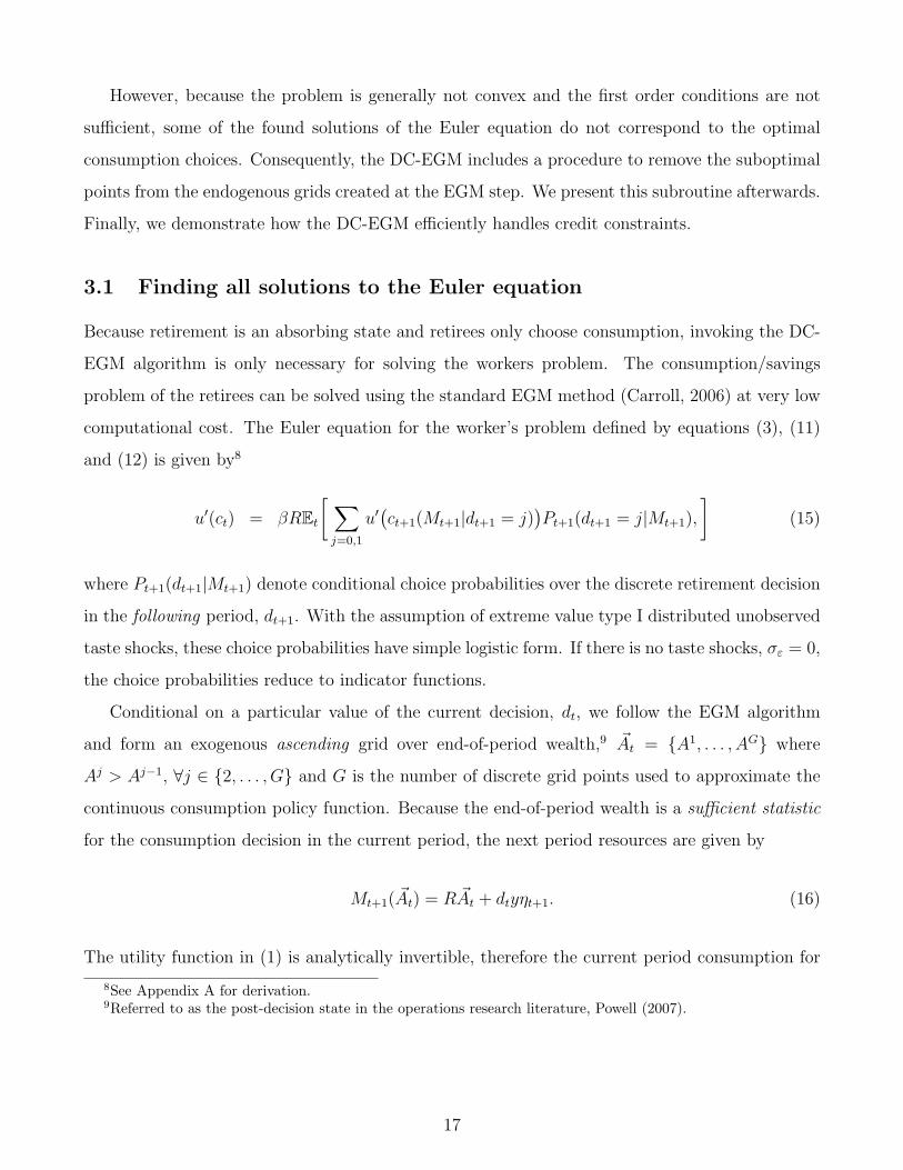
3.1 Finding all solutions to the Euler equation

Because retirement is an absorbing state and retirees only choose consumption, invoking the DC-

EGM algorithm is only necessary for solving the workers problem. The consumption/savings

problem of the retirees can be solved using the standard EGM method (Carroll, 2006) at very low

computational cost. The Euler equation for the worker’s problem defined by equations (3), (11)

and (12) is given by8

u′(ct) = βREt

[ ∑j=0,1

u′(ct+1(Mt+1|dt+1 = j))Pt+1(dt+1 = j|Mt+1),

](15)

where Pt+1(dt+1|Mt+1) denote conditional choice probabilities over the discrete retirement decision

in the following period, dt+1. With the assumption of extreme value type I distributed unobserved

taste shocks, these choice probabilities have simple logistic form. If there is no taste shocks, σε = 0,

the choice probabilities reduce to indicator functions.

Conditional on a particular value of the current decision, dt, we follow the EGM algorithm

and form an exogenous ascending grid over end-of-period wealth,9 At = {A1, . . . , AG} where

Aj > Aj−1, ∀j ∈ {2, . . . , G} and G is the number of discrete grid points used to approximate the

continuous consumption policy function. Because the end-of-period wealth is a sufficient statistic

for the consumption decision in the current period, the next period resources are given by

Mt+1(At) = RAt + dtyηt+1. (16)

The utility function in (1) is analytically invertible, therefore the current period consumption for

8See Appendix A for derivation.9Referred to as the post-decision state in the operations research literature, Powell (2007).

17

all discrete labor market choices dt can be calculated directly using the inverted Euler equation

ct(At|dt) = (u′)−1(βrhs

(Mt+1(At)

)), (17)

where rhs(Mt+1(At)

)is the right hand side of (15) evaluated at the pointsMt+1(At) using the next

period optimal consumption rules ct+1(Mt+1|dt+1). Finally, combining the current consumption

ct(At|dt) found in (17) with the points of At we get the endogenous grid over the current period

wealth

Mt(At) = ct(At|dt) + At. (18)

Finally, evaluating the maximand of the equation (12) at the points ct(At|dt), we compute the

choice specific value function vt(Mt(At)|dt

).

Algorithm 1 provides a pseudo-code of the described part of the DC-EGM which we call the

EGM step. The current period discrete choice, dt, and the next period policy and value functions

are inputs to this routine, while the endogenous grid Mt = Mt(At|dt) and the dt-specific consump-

tion and value functions, ct(Mt|dt) = ct(At|dt) and vt(Mt|dt

)= vt

(Mt(At)|dt

)computed on this

grid are the outputs.

Figure 5 plots a selection of values of vt(Mt|dt

)and ct(Mt|dt) against the endogenous grid Mt.

The points are indexed in the ascending order of the end-of-period wealth forming the grid At. The

solid lines approximate the corresponding functions with linear interpolation. It is evident that

the interpolated discrete choice specific value function vt(M |dt

)is a correspondence rather than a

function of M because of the existence of the region where multiple values of vt(M |dt

)correspond

to a single value of M . The same is true for the interpolated discrete choice specific consumption

function. The right and the left panels of Figure 5 illustrate the setting with and without the taste

shocks respectively. Adding taste shocks with a relatively low variance, σε = 0.03, reduces the size

of the regions with multiple corresponding values. Dashed lines illustrate discontinuities.

The region where multiple values of vt(M |dt

)correspond to a single value of M is the clear

evidence of non-concavity of the value function in the following period, and subsequent multiplicity

of solutions of the Euler equation. The EGM step approximates all solutions to the Euler equation

(see Lemma 2 in Appendix A), but because some of these solutions do not correspond to the optimal

choices, the value function correspondence has to be cleaned of the suboptimal points to obtain

actual value function. We should emphasize, however, that the points produced by the EGM step

18

Figure 5: Non-concave regions and the elimination of the secondary kinks in DC-EGM.

Value function (transformed)(a) σε = 0

24 26 28 30 32 34 36 38

0.0448

0.0449

0.045

0.0451

0.0452

0.0453

0.0454

0.0455

0.0456

0.0457

0.0458

[12]

[13]

[14]

[15]

[16]

[17]

[18]

[19]

[20]

[21]

[22]

[23]

[24]

Resources, M

Val

ue fu

nctio

n (t

rans

form

ed)

EGM−step: all solutionsDC−EGM

(b) σε = 0.03

24 26 28 30 32 34 36 38

0.0448

0.0449

0.045

0.0451

0.0452

0.0453

0.0454

0.0455

0.0456

0.0457

0.0458

[12]

[13]

[14]

[15]

[16]

[17][18]

[19]

[20][21]

[22]

[23]

[24]

Resources, M

Val

ue fu

nctio

n (t

rans

form

ed)

EGM−step: all solutionsDC−EGM

Consumption(c) σε = 0

24 26 28 30 32 34 36 3815

16

17

18

19

20

21

22

23

24

25

26

[11][12]

[13][14]

[15][16]

[17][18]

[19]

[20][21]

[22][23]

[24]

[25]

Resources, M

Con

sum

ptio

n, c

EGM−step: all solutionsDC−EGM

(d) σε = 0.03

24 26 28 30 32 34 36 3815

16

17

18

19

20

21

22

23

24

25

26

[11][12]

[13][14]

[15][16] [17]

[18]

[19]

[20]

[21] [22][23]

[24][25]

Resources, M

Con

sum

ptio

n, c

EGM−step: all solutionsDC−EGM

Notes: The plots illustrate the output from the EGM-step of the DC-EGM algorithm (Algorithm 1) in a non-concave

region. The dots are indexed with the index j of the ascending grid over the end-of-period wealth At = {A1, . . . , AG}where Aj > Aj−1, ∀j ∈ {2, . . . , G}. The connecting lines show the dt-specific value functions vt(Mt|dt) and the

consumption function ct(Mt|dt) linearly interpolated on the endogenous grid Mt. computed on this grid are the

outputs. The left panels illustrate the deterministic case without taste shocks, while in the right panels σε = 0.03.

The “true” solution, after applying the DC-EGM algorithm is illustrated with a thick solid red line. Dashed lines

illustrate discontinuities. The solution is based on G = 70 grid points in At, R = 1, β = 0.98, y = 20, ση = 0.

19

Algorithm 1 The EGM-step: dt choice-specific consumption and value functions

1: Inputs: Current decision dt. Choice-specific consumption and value functions ct+1(Mt+1|dt+1) and

vt+1(Mt+1|dt+1) associated with the endogenous grid in period t+ 1, Mt+1

2: Let η = {η1, . . . , ηQ} be a vector of quadrature points with associated weights, ω = {ω1, . . . , ωQ}3: Form an ascending grid over end-of-period wealth, At = {A1

t , . . . , AGt } where Aj

t > Aj−1t , ∀j ∈ {2, . . . , G}

4: for j = 1, . . . , G do (Loop over points in At)5: for q = 1, . . . , Q do (Loop over quadrature points in η)6: Compute Mq

t+1(Aj) = RAj + dtyη

qt+1

7: for dt+1 = 0, 1 do

8: Compute ct+1(Mqt+1(A

j)|dt+1) by interpolating ct+1(Mt+1|dt+1) at the point Mqt+1(A

j)

9: Compute vt+1

(Mq

t+1(Aj)|dt+1

)by interpolating vt+1(Mt+1|dt+1) at the point Mq

t+1(Aj)

10: end for11: Compute ϕt+1

(Mq

t+1(Aj))= σε log

(∑j=0,1 exp(vt+1

(Mq

t+1(Aj)|dt+1 = j

))/σε

)12: Compute Pt+1(dt+1|Mq

t+1(Aj)) = exp(vt+1

(Mq

t+1(Aj)|dt+1

)/σε)(

∑j=0,1 exp(vt+1

(Mq

t+1(Aj)|dt+1 = j

))/σε)

−1

13: end for14: Compute rhs

(Mt+1(A

j))= βR

∑Qq=1

∑j=1,2 ω

q · u′(ct+1(Mqt+1(A

j)|dt+1 = j))· Pt+1(dt+1 = j|Mq

t+1(Aj))

15: Compute expected value function EVt+1

(Mt+1(A

j))=∑Q

q=1 ωq · ϕt+1

(Mq

t+1(Aj))

16: Compute current consumption ct(Aj |dt) = u′−1

(rhs

(Mt+1(A

j)))

17: Compute value function vt(Mt(A

j)|dt)= u(ct(A

j |dt)) + βEVt+1

(Aj)

18: Compute endogenous grid point Mt(Aj |dt) = ct(A

j |dt) +Ajt

19: end for20: Collect the points Mt(A

j |dt) from the endogenous grid Mt = {Mt(Aj |dt), j = 1, . . . , G} associated with

the choice-specific consumption and value functions: ct(Mt|dt

)= {ct

(Mt(A

j)|dt), j = 1, . . . , G} , and

vt(Mt|dt

)= {vt

(Mt(A

j)|dt), j = 1, . . . , G}

21: Outputs: Mt, ct(Mt|dt) and vt(Mt|dt

)Notes: The pseudo code is written under the assumption that quadrature rules are used for calculating the expec-

tations, whereas particular implementations can employ other methods for computing the expectation. It is also

assumed that interpolation rather than approximation is used in Steps 8 and 9, although the latter is also possible.

necessarily contain the true solutions. This is a notable contrast to the standard solution methods

based on an exogenous grid over wealth, which may struggle to find the points of optimality and

have to deploy computationally costly global search methods to solve the optimization problem in

the Bellman equation.

The next section describes a procedure in DC-EGM algorithm that deals with selecting the

true optimal points among the points produced by the EGM step. The true solution found by the

full DC-EGM algorithm is illustrated in Figure 5 with a red line for reference.

3.2 Calculation of the Upper Envelope

To distinguish between the optimal and suboptimal points produced by the EGM step, the DC-

EGM algorithm makes a direct comparison of the values associated with each of the choices. On

20

the plots of the discrete choice specific value function correspondences in Figure 5 (panels a and

b), this amounts to computing the upper envelope of the correspondence in the regions of Mt where

multiple solutions are found.

To provide deeper insight into this process, we plot the maximand of the equation (12) that

defines the discrete choice specific value function vt(Mt|dt) in Figure 6 as a function of consumption

cguess for various values of Mt. The value of vt(Mt|dt) is the global maximum of the this function.

The EGM step (Algorithm 1), however, recovers all critical points where the derivative of the

plotted function is zero.10 The same points in Figures 6 and 5 are indexed with the same indexes

for easy comparison.

Figure 6: Local maxima and multiple solutions of the Euler equation.

(a) σε = 0

16 18 20 22 24 260.0451

0.0451

0.0452

0.0452

0.0453

0.0453

0.0454

0.0454

0.0455

Consumption, cguess

Can

dida

te v

alue

func

tion

(tra

nsfo

rmed

)

[15]

[23]

[16]

M=29.9

M*=30.6

M=31.3

M=32.4

(b) σε = 0.03

16 18 20 22 24 260.0451

0.0452

0.0452

0.0453

0.0453

0.0454

0.0454

0.0455

0.0455

Consumption, cguess

Can

dida

te V

alue

func

tion

(tra

nsfo

rmed

)

[15]

[23]

[19]

[16]

M=29.9

M*=30.5

M=31.2

M=32.5

Notes: The figure plots the maximand of the equation (12), which defines the discrete choice specific value function

vt(Mt|dt = 1), for the case of σε = 0 (panel a) and σε = 0.03 (panel b). Horizontal lines indicate the critical points

found or approximated by the EGM step of DC-EGM algorithm. The points are indexed with the same indexes as

in Figure 5 and the black dots represent global maxima. Model parameters are identical to those of Figure 5.

In the case without taste shocks, σε = 0 (panel a), two levels of consumption satisfy the Euler

equation (15) in the range Mt ∈ [27, 36]. From Figure 5 we know that points indexed 16 to 21 are

suboptimal. Panel (a) in Figure 6 illustrates that the maximand function computed for wealth

10More specifically, because the grid At is finite, for every distinct point of the endogenous grid Mt = Mt(At)it recovers one of the local maxima that corresponds to one of the solutions to the Euler equation. The otherlocal maxima are approximated by interpolation of the value function correspondence between the points of theendogenous grid Mt = Mt(At).

21

Mt in this range has two local maxima. For example, the 15th point from the EGM step is the

global maximum of the maximand computed at Mt ≈ 29.9, while the 16th point is not the global

maximum when resources are Mt ≈ 31.3.

At some point, the two solutions originating from the two segments of the value function

correspondence are both optimal. Around Mt ≈ 30.6 in panel (a) of Figure 6, the decision maker

is indifferent between the discrete choices (at the next or some future periods – depending on

whether the multiplicity of the solutions was caused by the primary or secondary kink of the next

period value function). At this point of indifference, the consumption function is discontinuous,

as illustrated with the red dashed line in panel (c) in Figure 5. The intersection point is not

necessarily found in the EGM-step outlined above and needs to be additionally computed.11

In the smooth case with σε = 0.03 the problem of multiplicity of local maxima in the maximand

of equation (12) is generally still present, as shown by panel (b) of Figure 6. Correspondingly,

there is still a discontinues drop in consumption around Mt around Mt ∈ [29, 31]. In other words,

the taste shocks with scale parameter σε = 0.03 do not fully “convexify” the value function. Note

that in the smooth case there can be three solutions to the Euler equation, only one of which is a

global maximum. This configuration is dealt with by the same upper envelope method.

It is clear, that selecting the global maximum among the critical points located by solving

the Euler equation during the EGM step amounts to comparing the values of the constructed

value function correspondence vt(Mt|dt) for each Mt. For comparison, the overlapping segments of

vt(Mt|dt) may have to be re-interpolated on some common grid, and the upper envelope has to be

computed. Algorithm 2 presents the pseudo-code of this calculation. The key insight of the upper

envelope algorithm is to use the monotonicity of the end-of-period resources as a function of wealth

to detect the regions where multiple values of choice-specific value function v(Mt|dt) are returned

for a single value of Mt (see Step 3 of Algorithm 2). Monotonicity of end-of-period wealth is due to

the concavity of the utility function as shown in Theorem 3, see Appendix A. Around every such

detected region, the value function correspondence is broken into three segments (Steps 5 to 7),

which are then compared point-wise to compute the upper envelope (Step 12). The inferior points

are simply dropped from the endogenous grid Mt, and optionally the approximated kink points at

the inserted. Consequently, the consumption and value function correspondences are cleaned up

and become functions.

11In presence of taste shocks, finding the precise indifference points is not essential, but in deterministic settingsfinding exact intersection points considerably increases the accuracy of the solution.

22

Algorithm 2 Upper envelope refinement step

1: Inputs: Endogenous grid Mt = Mt(At) obtained from the grid over the end-of-period resources

At = {A1, . . . , AG} where Aj > Aj−1, ∀j ∈ {2, . . . , G}; saving and value function correspondences ct(Mt|dt)and vt

(Mt|dt

)computed on Mt

2: for j = 2, . . . , G do (Loop over the points of endogenous grid)3: if Mt(A

j) < Mt(Aj−1) then (Criterion for detecting non-concave regions)

4: Find the first h ≥ j such that Mt(Ah) < Mt(A

h+1)5: Let J1 = {j′ : j′ ≤ j − 1} (Points up to [19] in panel a and [17] in panel b of Figure 5)6: Let J2 = {j′ : j − 1 ≤ j′ ≤ h} (Points [19], [20] in panel a and [17]-[20] in panel b of Figure 5)7: Let J3 = {j′ : h ≤ j′} (Points [20] and up in both panel a and b of Figure 5)

8: Let M ′ = {Mt(Aj′) : mini∈J2 Mt(A

i) = Mt(Ah) ≤ Mt(A

j′) ≤ Mt(Aj−1) = maxi∈J2 Mt(A

i)}9: for i = 1, . . . , |M ′| do where |M ′| is the number of points in M ′

10: Denote vt(Mt|dt, Jr

)the segment of vt

(Mt|dt

)computed on the points in the set Jr

11: Interpolate the segments vt(Mt|dt, Jr

)at the point Mt(A

i) if i /∈ Jr, r = 1, . . . , 3

12: if vt(Mt(A

i)|dt)< maxr vt

(Mt(A

i)|dt, Jr)then

13: Drop point i from the endogenous grid Mt

14: end if15: end for16: Find the point M× : vt

(M×|dt, J3

)= vt

(M×|dt, J1

)[Optional]

17: Insert M× into Mt first with associated values vt(M×|dt, J3

)and ct

(M×|dt, J3

)[Optional]

18: Insert M× into Mt then with associated values vt(M×|dt, J1

)and ct

(M×|dt, J1

)[Optional]

19: Set j = h20: else21: Keep point j on the endogenous grid Mt as is22: end if23: end for24: Outputs: Refined endogenous grid Mt, consumption and value functions ct(Mt|dt) and vt

(Mt|dt

)Note: The pseudo code is written using an elementary algorithm for calculation of the upper envelope for a collection

of functions defined on their individual grids. More efficient implementations could also be used, see for example

(Hershberger, 1989). Inserting the intersection point M× into the endogenous grid Mt two times in step 17 and 18

ensures an accurate representation of the discontinuity in consumption function ct(Mt|dt). If the optional steps 16-

18 are skipped, the secondary kink is smoothed out, but the overall shapes of the consumption and value functions

are correct.

While the DC-EGM is similar to the approach proposed in Fella (2014), we explicitly allow for

extreme value type I taste shocks to preferences and show how they help with the computational

issues specific to the model of discrete-continuous choices. The approach in Fella (2014) does

not readily apply to the class of models with taste shocks but should be adjusted along the lines

described here. Particularly, the DC-EGM operates with discrete choice specific value functions

and optimal consumption rules, and computes integrals of smooth objects. Furthermore, contrary

to Fella (2014) who uses instances of increasing marginal utility to detect non-concave regions,

DC-EGM uses the value function correspondence. However, both approaches rely on monotonicity

of the optimal end-of-period savings function.

23

Algorithm 3 The DC-EGM algorithm

1: In the terminal period T fix a grid MT over the consumable wealth MT . On this grid compute consumptionrules cT (MT |dT ) = MT and value functions vT (MT |dT ) = (log(MT ) − dT ) for every value of discrete choicesdT . This provides the base for backward induction in time

2: for t = T − 1, . . . , 1 do (Loop backwards over the time periods)3: for j = {0, 1} do (Loop over the current period discrete choices)

4: Invoke the EGM step (Algorithm 1) with dt = j, ct+1(Mt+1|dt+1) and vt+1(Mt+1|dt+1) as inputs

5: Invoke upper envelope (Algorithm 2) using outputs from Step 4, Mt, ct(Mt|dt) and vt(Mt|dt

)as inputs

6: The endogenous grid Mt and consumption and value functions ct(Mt|dt) and vt(Mt|dt

)are now computed

7: end for8: end for9: The collection of the choice-specific consumption and value functions ct(Mt|dt) and vt(Mt|dt) defined on the

endogenous grids Mt for dt = {0, 1} and t = {1, . . . , T} constitutes the solution of the consumption/savings andretirement model

Algorithm 3 presents the pseudo-code of the full DC-EGM algorithm, which invokes the EGM

step (Algorithm 1) repeatedly to compute the value function correspondences for all discrete

choices, and then finds and removes all suboptimal points on the returned endogenous grids by

calling the upper envelope module (Algorithm 2).

An important question of how the method handles the situations when the non-convex regions

go undetected due to relatively coarse grid At is addressed by the Monte Carlo simulations in the

next section. We show that even with small number of endogenous grid points the Nested Fixed

Point (NFXP) Maximum Likelihood estimator based on the DC-EGM algorithm performs well

and is able to identify the structural parameters of the model.

3.3 Credit Constraints

Before turning to the Monte Carlo results, we briefly discuss how DC-EGM handles the credit

constraints, ct ≤ Mt. During the EGM step, the credit constraints are dealt with in exactly same

manner as in Carroll (2006). Let the smallest possible end-of-period resources A1 = 0 be the first

point in the grid At. Assuming that the corresponding point of the endogenous grid Mt(A1|dt) is

positive12, it holds that At(M |dt) = 0 for all M ≤ Mt(A1|dt) due to the monotonicity of saving

function At(M |dt) = M − ct(M |dt) (see Theorem 3 in Appendix A). Therefore, the optimal

consumption in this region is then given by ct(M |dt) = M , and the choice-specific value function

is

vt(M |dt) = log(M)− dtδt + β

∫EVt+1(dtyηt+1)f(dηt+1), M ≤ Mt(A

1|dt). (19)

12It is not hard to show that this holds as long as the per period utility function satisfies the Inada conditions.

24

Note that the third component of (19) is the expected value of having zero savings. It is calculated

within the EGM step for the point A1 = 0, and should be saved separately as a constant that

depends on dt but not on Mt. Once this constant is computed, vt(M |dt) essentially has analytical

form in the interval [0,Mt(A1|dt)], and thus can be directly evaluated at any point.

When the per-period utility function is additively separable in consumption and discrete

choice like in the retirement model we consider, (19) holds for all dt ∈ Dt in the interval

0 ≤ M ≤ mindt∈Dt Mt(A1|dt). In other words, the choice specific value functions for low wealth

have the same shape (in our case log(M)), which is shifted vertically with dt-specific coefficients.

This implies that the logistic choice probabilities Pt(dt|Mt) are constant in this interval, and have

to only be calculated once.

4 Monte Carlo Results

In this section we investigate the properties of the approximate maximum likelihood estimator

(MLE) that we obtain using the DC-EGM to approximate the model solution in the inner loop

of the Nested Fixed Point algorithm. We specifically focus on role of income uncertainty and

taste shocks for the approximation bias induced by a numerical solution with a finite number of

grid-points; in particular how approximation bias depends on the number of grid points in smooth

as well as non-smooth problems. After a description of the data generating process (DGP), we

present the results from a series of Monte Carlo experiments, and show that models used in

typical empirical applications are sufficiently smooth to almost eliminate approximation bias using

relatively few grid points.

4.1 Data Generation Process

For the Monte Carlo we consider a slightly more general formulation of the consumption/savings

and retirement problem defined in (1) with constant relative risk aversion (CRRA) utility

max{ct,dt}T1

T∑t=1

βt

(c1−ρt − 1

1− ρ− δtdt

)(20)

where ρ is the CRRA coefficient.

In order to simulate synthetic data from the DGP consistent with the model and the vector

25

Table 1: Baseline true parameter values.

Description Value Description ValueTime horizon T = 44 Disutility of work δ = 0.5Gross interest rate R = 1.03 Discount factor β = 0.97Full time employment income y = 1.0 CRRA coefficient ρ = 2.0Income variance ση = 0 Taste shocks scale σε ∈ {0.01, 0.05}

of true parameter values, we solve the model very accurately with 2,000 grid points using the DC-

EGM. We refer to this solution as the true solution even though this is off course only an accurate

finite approximation of the value function.13

We consider several specifications of the model in the Monte Carlo experiments below to study

various aspects of the performance of the estimator. Once again, we assume that disutility of work

is constant over time, i.e. δt = δ. Table 1 presents the parameter values in the baseline specification

of the model. Deviations are given explicitly with every Monte Carlo experiment separately. We

perform 200 replications for each combination of settings.

For each specification of the model, 50,000 individuals are simulated for T = 44 periods. Each

individual i is initiated as full-time worker sdi,1 = 1, where we have used sdi,t ∈ {0, 1} to denote

the labor market state, i.e. whether an individual is retired (sdi,t = 0) or working (sdi,t = 1). Each

workers initial wealth Mdi,1 is drawn from a uniform distribution on the interval [0, 100]. At the

beginning of each time period t, a random log-normal labor market income shock ηt with variance

parameter ση is drawn if the individual i is working and individual’s resources Mdt are calculated.

Given the level of resources, discrete-choice specific value functions and choice probabilities are

computed, and a random draw determines which discrete labor market option ddit is chosen. After

one period lag, the labor force participation decision becomes the labor market state, sdi,t+1 = ddit.

The optimal level of consumption, cit, is then computed conditional on ddit, and the end-of-period

wealth is calculated and stored to be used for calculation of resources available in the beginning

of period t + 1, Mdi,t+1. We then add normal additive measurement error with standard devi-

ation σξ = 1 to get the simulated consumption data, cdit. This produces simulated panel data

(Mdit, s

dit, d

dit, c

dit) for each individual i ∈ {1, . . . , 50, 000} in all time periods t ∈ {1, . . . , 44}.

13As a spot check, we have also compared this solution with the traditional value function iteration approach,where we used a grid search over 1,000 discrete points on the interval [0,Mt] to locate the optimal consumption foreach value of wealth. We find that results are essentially identical.

26

4.2 Maximum Likelihood Estimation

We implement a discrete-continuous version of the Nested Fixed Point (NFXP) Maximum Likeli-

hood estimator devised in Rust (1987, 1988), where we augment the original discrete-choice esti-

mator with a measurement error approach when assessing the likelihood of the observed continuous

choices.

Assume that a panel dataset is available, {(Mdit, s

dit, d

dit, c

dit)}i={1,...,N}, t={1,...,T}, containing obser-

vations on wealth, labor market state, discrete and continuous choices of individuals i = 1 . . . , N

in time periods t = 1, . . . , T . Let ct(Mt, st, dt|θ) denote the consumption policy function computed

by the DC-EGM for a given vector of model parameters θ = (δ, β, ρ, ση, σε). We assume that

consumption is observed with additive Gaussian measurement error,

cdit = ct(Mdit, s

dit, d

dit|θ) + ξit, ξit ∼ N(0, σξ), i.i.d. ∀i, t. (21)

Let ξdit(θ) = cdit − ct(Mdit, s

dit, d

dit|θ) denote the difference between the predicted and the observed

consumption. We assume that the measurement error, ξit, is independent of the taste shocks,

εt(dt), and, thus, the joint likelihood of observation i in period t is given by

ℓit(θ, σξ) = P (ddit|Mdit, s

dit, θ)

ϕ(ξdit(θ)/σξ)

σξ

, (22)

where ϕ(·) is the density function of the standard normal distribution. We have ignored the

controlled transition probability for the retirement status sdit, since Ptr(sdit|sdi,t−1, d

di,t−1) is always 1

in the data when retirement is absorbing and the labor market state is perfectly controlled by the

decision.

The choice probabilities for the workers (sdit = 1) are standard logits

P (ddit|Mdit, s

dit, θ) =

exp(vt(Mdit, s

dit, d

dit|θ)/σε)∑1

j=0 exp(vt(Mdit, s

dit, j|θ)/σε)

(23)

and are computed from the discrete choice specific value functions vt(Mdit, s

dit, d

dit|θ) found by the

DC-EGM given a particular value of the parameter vector θ, evaluated at the data. Because retire-

ment is absorbing and thus retirees do not have any discrete choice to make, the first component

of individual likelihood contribution (22) drops out when sdit = 0.

The joint log-likelihood function is given by L(θ, σξ) = log∏N

i

∏Tt ℓit(θ, σξ) where re-arranging

27

the first order condition with respect to σ2ξ yields the standard ML estimator for the measurement

error variance, σ2ξ (θ) = 1

NT

∑Ti

t=1 ξdit(θ)

2. The concentrated log-likelihood function is, therefore,

proportional to

L(θ) ∝N∑i=1

T∑t=1

{sditσε

(vt(M

dits

dit, d

dit|θ)− EVt(M

dit, s

dit|θ)

)− 1

2log

(N∑i=1

T∑t=1

ξdit(θ)2

)}, (24)

where EVt(Mdit, s

dit|θ) is the the logsum given in (13) evaluated at parameter value θ.14 The

parameter vector θ that maximizes (24) is the ML estimator of the model parameters.

4.3 Taste Shocks as Unobserved State Variables

We are now ready to investigate the effects of smoothing on the accuracy of the ML estimator

based on the DC-EGM algorithm. We conduct two Monte Carlo experiments where we vary the

degree of smoothing induced by extreme value taste shocks and income uncertainty respectively.

Throughout, we focus on estimating the parameter that index disutility of work, δ, while keeping

all other fixed at their true values. The Appendix D contains average estimation time for the

DC-EGM.

Taste Shocks and Approximation Error. Figure 7 displays the root mean square error

(RMSE) of the parameter estimates for the disutility of work, δ. Results are shown for varying

degree of smoothing, σε ∈ {0.01, 0.05}, and different values of the disutility of work parameter,

δ ∈ {0.1, 0.5}. With RMSE around 1.0e−3, the proposed estimator is already accurate with 50 grid

points and rapidly improves as the number of grid points increase from 50 through 1000. Note

that standard errors will of course increase with σε due to the increased amount of unexplained

variation in the error term and RMSE reflects this too. Bearing this is mind, it is evident that the

approximation bias decreases as the degree of smoothing increases, i.e., larger values of σε. For

higher levels of smoothing, problems with multiplicity of the Euler equation solutions disappear and

few grid points are needed to approximate the (smooth) consumption function. This is particularly

true when the disutility from work is large (δ = .5) because the non-concave regions are larger

in this case. We also calculated the Monte Carlo Standard Deviation (MCSD)15, which is on the

order 1.0e−4 irrespectively of the number of grid points used.

14Following (24), the logsum only has to be evaluated for workers, sdit = 1.15MCSD results not shown

28

Figure 7: Monte Carlo results: disutility of work.

(a) δ = 0.1

0 200 400 600 800 10000

1

2

3

4x 10−3

# of gridpoints

RM

SE

σε = 0.01σε = 0.05

(b) δ = 0.5

0 200 400 600 800 10000

1

2

3

4x 10−3

# of gridpoints

RM

SE

σε = 0.01σε = 0.05

Notes: The plots illustrate the root mean square error (RMSE) of δ. Results are shown for varying degree of

smoothing, σε ∈ {0.01, 0.05}, and different values of the disutility of work, δ ∈ {0.1, 0.5}. The rest of the parameters

are at their baseline levels, see Table 1.

Income Uncertainty. Additional uncertainty about, e.g., future labor market income tend

to smooth out secondary kinks stemming from multiple solutions to the Euler equations. To

illustrate how that additional smoothing affects the proposed estimator, Figure 8 display RMSE

when introducing income uncertainty. We report results from two different values of the income

variance16, σ2η ∈ {0.001, 0.05}. The first level, 0.001, does not completely smooth out secondary

kinks while the significantly more uncertain income process with σ2η = 0.05 does (see the right

panel of Figure 3).

Income uncertainty together with taste shocks smooth the problem to such a degree that

the RMSE drops by an order of magnitude when increasing the income variance from .001 to

0.05. Hence, using only few grid points when estimating such a model will result in only minor

approximation errors.

As mentioned, standard errors will of course increase with σε due to the increased amount

of unexplained variation. The MCSD is quite small and unaffected by the degree of income

uncertainty as well as the number of grid points, but increases from 0.00023 to 0.00045 as σε

increases from 0.01 to 0.05. This is the main explanation for why RMSE is only smaller for a small

16The values of the income variance we use correspond well to the empirical findings, for example inGourinchas and Parker (2002); Meghir and Pistaferri (2004); Imai and Keane (2004).

29

Figure 8: Monte Carlo results: income uncertainty.

(a) σ2η = 0.001

0 100 200 300 400 5000

1

2

3

4x 10−3

# of gridpoints

RM

SE

σε = 0.01σε = 0.05

(b) σ2η = 0.05

0 100 200 300 400 5002

4

6

8

10

12

14x 10−4

# of gridpoints

RM

SE

σε = 0.01σε = 0.05

Notes: The plots illustrate the root mean square error (RMSE). Results are shown for varying degree of smoothing,

σε ∈ {0.01, 0.05}, and different values of the income variance, σ2η ∈ {0.001, 0.05}. The rest of parameters are at

their baseline levels, see Table 1.

number of grid points. Sorting out this effect its clear that increasing σε decreases the amount of

pure approximation bias - especially when the number of grid points is small. Note that MCSD

is very small, in part due to a relatively large sample size, but also because the variance of the iid

extreme value error term is extremely small. In most empirical applications, σε would be larger;

leading to an even smoother problem than the one we consider here. Hence, with relatively few

grid points we can expect to obtain an even smaller approximation bias induced by the finite grid

approximation in the DC-EGM.

4.4 Taste Shocks as Logit Smoother

Until now we have assumed that the correct model has unobserved state variables, and thus σε > 0

has to be estimated. To investigate how the proposed estimator performs if the data stems from a

model in which there are no unobserved states, we estimate versions of the model where we impose

σε > 0 and, thus, estimate a misspecified model. This is interesting because if researchers have

reasons to believe that the underlying model has no shocks, the inclusion of these shocks acts as

a smooth approximation to the true deterministic model. As argued above, solving the smoothed

model is much faster since it requires fewer grid points and, thus, is much faster to estimate.

Figure 9 illustrates the RMSE when using 50, 100 and 500 grid points for various levels of

30

smoothing σε ∈ [0.001, 0.05] while the correct level is σε = 0. Intuitively, as the model becomes

“more” misspecified (increasing the imposed σε), the RMSE and the MCSD increases. Interestingly,

for a given number of discrete grid points, the RMSE is minimized by a σε > 0. While large degree

of smoothing induces significant approximation bias, the bias is initially falling in σε until some

point at which the RMSE increases again. The minimum of the RMSE is attained for lower levels of

smoothing if additional stochasticity (i.e. income shocks) is present in the model. This is expected

because the income uncertainty smooths the problem and less logit smoothing is needed to obtain

the optimal smooth approximation. It is worth noting, however, that the optimal amount of logit

smoothing may not be sufficient to completely eliminate the non-convexities in the model. It is

therefore essential for the solution method to be able to robustly solve optimization problems with

multiple local solutions, the task that DC-EGM performs particularly well.

These results show the potential for great speed gains by smoothing. Using only 50 grid points

and imposing σε = 0.01 produce a RMSE of around the same level as using 500 grid points and

imposing σε ≈ 0 close to the true model. We can reduce the number of gridpoints by an order

of magnitude without increasing the root mean square error significantly simply by choosing the

degree of smoothing appropriately. Note, however, that there is naturally a trade-off between

lowering the computational cost by increasing smoothing and decreasing the number of grid points

and the accuracy of the resulting solution compared to the true solution of the non-smooth model.

5 Discussion and Conclusions

In this paper we have shown how complications from numerous discontinuities in the consumption

function to a life cycle model with discrete and continuous choices can be avoided by smoothing the

problem and using the DC-EGM algorithm. The proposed algorithm retains all the nice features

of the original EGM method, namely that it typically does not require any iterative root-finding

operations, and is equally efficient in dealing with borrowing constraints. Moreover, we show that

the smoothed model can be successfully estimated by the NFXP estimator based on the DC-EGM

algorithm even with small number of grid points, and even when the true DGP is non-smooth.

For expositional clarity, we focused on a simple illustrative example when explaining the details

of the DC-EGM algorithm. This also allows us to derive an analytical solution that we can

compare to the numerical one. The analytical solution provides economic intuition for why first

31

Figure 9: Monte Carlo results: true model without taste shocks (misspecified)

Root mean square error(a) 50 grid points

0 0.01 0.02 0.03 0.04 0.050

0.005

0.01

0.015

0.02

σε

RM

SE

σ2

η= 0

σ2

η= 0.05

(b) 100 grid points

0 0.01 0.02 0.03 0.04 0.050

0.005

0.01

0.015

0.02

σε

RM

SE

σ2

η= 0

σ2

η= 0.05

(c) 500 grid points

0 0.01 0.02 0.03 0.04 0.050

0.005

0.01

0.015

0.02

0.025

σε

RM

SE

σ2

η= 0

σ2

η= 0.05

Notes: The plots illustrate the root mean square error (RMSE) from estimation of a misspecified model. The model

from which data are simulated is deterministic, σε = 0, while the model used to estimate the disutility of work

imposes σε > 0. Results are shown for varying degree of imposed smoothing, σε ∈ [0.001, 0.05] on the horizontal

axes, different levels of income shocks, ση ∈ {0, 0.05}, and different number of grid points. The rest of parameters

are at their baseline levels, see Table 1.

and second order kinks appear and permits direct evaluation of the precision of the DC-EGM

algorithm. Admittedly, the illustrative model of consumption and retirement is very stylized, and

the reader may wonder if DC-EGM can be used to solve and estimate larger, more complex and

realistic models with more state variables, multiple discrete alternatives, heterogeneous agents,

institutional constraints, etc.. The answer is positive. As shown in the Appendix A, the DC-EGM

method can be applied to a much more general class of problems as long as the post decision state

variable is a sufficient static for the continuous choice in the current period, and the marginal utility

function and intra-temporal budget constraint are invertible. When the marginal utility function

is analytically invertible, DC-EGM also avoids the bulk of costly root-finding operations.17

The DC-EGM method has been implemented in several recent empirical applications, where it

has proven to be a powerful tool for solving and estimating more complex DC models in various

fields: labor supply, human capital accumulation and saving (Iskhakov and Keane, 2016); joint

retirement decision of couples (Jørgensen, 2014); consumption, housing purchases and housing debt

(Yao, Fagereng and Natvik, 2015); saving decisions and fertility (Ejrnæs and Jørgensen, 2015);

precautionary borrowing and credit card debt (Druedahl and Jørgensen, 2015).

17DC-EGM algorithm can also be generalized for other specifications including the models with large statespace and multidimensional discrete choice. White (2015); Iskhakov (2015); Druedahl and Jørgensen (2016) presenttheoretical foundations for extending endogenous grid methods to multi-dimensional models.

32

We have demonstrated in the Monte Carlo experiments that the NFXP maximum likelihood

estimator based on the DC-EGM solution algorithm performs very well when decisions are made

under uncertainty, e.g. in the presence of extreme valued taste shocks and the existence of income

uncertainty. Even when the true model is deterministic, taste shocks can be used as a powerful

smoothing device to simplify the solution without much approximation bias due to over-smoothing.

The addition of extreme value taste shocks is not only a convenient smoothing device that

simplifies the solution of DC models, it is also an empirically relevant extension required to avoid

statistical degeneracy of the model. In empirical applications the variance of these shocks is

typically much larger compared to what we have considered here. This makes models smooth

enough to almost eliminate approximation bias in parameter estimates even with relatively few

grid points. We therefore conclude that DC-EGM is both practical and appears to be a fast and

accurate method for use in actual empirical applications.

However from the standpoint of using DC-EGM to find highly accurate solutions to DC prob-

lems, while the results we present in this paper are highly encouraging, our conclusions are based

on comparing the numerical solution to an analytical solution of a particular DC problem. It

would be much better to be able to prove that DC-EGM provides similar accuracy for an entire

class of DC problems. Ideally this would be done by deriving bounds on the error between the true

decision rule and the approximate decision rule computed by DC-EGM. We conjecture that these

bounds, dependent on the number of endogenous gridpoints n used in the DC-EGM algorithm,

would converge to zero as n → ∞. We are not aware of any error bounds or convergence proofs

even in more straightforward case of concave dynamic problems with only continuous choice that

EGM was originally developed for by Carroll (2006). We believe the uniform bounds we derived

for the approximation error involved in the use of extreme value smoothing of DC problems may

provide one of the tools to derive bounds on the error between the true decision rules and the

approximate decision rules calculated by DC-EGM.

A Theoretical foundations of DC-EGM

For the purpose of this Appendix we consider the following more general formulation of the con-sumption/savings and retirement problem. Let Mt denote consumable wealth that is continuousstate variable with particular motion rule described below, and let st denote a vector of additionaldiscrete or discretized state variables. Let ct be the scalar continuous decision (consumption) anddt be a scalar discrete decision variable with finite set of values that could encode multiple dis-

33

crete decisions if needed. Consider the dynamic discrete-continuous choice problem given by theBellman equation,

Vt(Mt, st) = max0≤ct≤Mt,dt∈Dt

[u(ct, dt, st) + σεεt(dt) + βtEt

{Vt+1(Mt+1, st+1)|At, dt

}], (25)

where t = 1, . . . , T − 1, and the last component of the maximand is absent for t = T . The choicesin the model are restricted by the credit constraint ct < Mt and feasibility sets Dt. The perperiod utility includes scaled taste shocks σεεt(dt), where εt is a vector of i.i.d. Extreme Value(Type I) distributed random variables. The dimension of εt is equal to the number of alternativesthat the discrete choice variable may take, εt(dt) denotes the component that corresponds to aparticular discrete decision. In the general case the discount factor βt is time-specific to allowfor the probability of survival. The expectation is taken over the taste shocks εt+1, transitionprobabilities of the state process st as well as any serially uncorrelated (or idiosyncratic) shocksthat may affect Mt+1 and st+1. The expectation is taken conditional on the choices in period tusing the sufficient statistic At = Mt − ct in place of the continuous (consumption) choice.

Using the well known representation of the expectation of the maximum of Extreme Value dis-tributed random variables, the Bellman equation (25) can be written in terms of the deterministicchoice-specific value functions vt(Mt, st|dt) as

vt(Mt, st|dt) = max0≤ct≤Mt

[u(ct, dt, st) + βtEt

{Vt+1(Mt+1, st+1)|At, dt

}](26)

= max0≤ct≤Mt

[u(ct, dt, st) + βtEt

{ϕ(vt+1(Mt+1, st+1|dt+1), Dt+1, σε

)|At, dt

}], (27)

where ϕ(xj, J, σ) = σ log[∑

j∈J expxj

σ

]is the logsum function. The expectation in (27) is now

only taken w.r.t. state transitions and idiosyncratic shocks, unlike in (25) and (26).The crucial assumption for the DC-EGM is that post decision state At constitutes the sufficient

statistic for the continuous choice in period t, i.e. that transition probabilities/densities of the stateprocess (Mt, st) depend on At rather than Mt or ct directly. It is also required that At as a functionof Mt is (analytically) invertible. For our case, assume for concreteness that At = Mt − ct, andthat Mt+1 = RAt + y(dt), where R is a gross return, and y(dt) is discrete choice specific income.We also assume that the utility function u(ct, dt, st) satisfies the following condition.

Assumption 1 (Concave utility). The instantaneous utility u (ct, dt, st) is concave18 in ct and has

a monotonic derivative w.r.t. ct that is (analytically) invertible.

Lemma 1 (Smoothed Euler equation). The Euler equation for the problem (25) takes the form

u′(ct, dt, st) = βtREt

∑dt+1∈Dt+1

u′(ct+1(Mt+1, st+1|dt+1), dt+1, st+1

)Pt+1

(dt+1|Mt+1, st+1

) (28)

where u′(ct, dt, st) is the partial derivative of the utility function w.r.t. ct, ct+1(Mt+1, st+1|dt+1) isthe choice-specific consumption function in period t+1, and Pt+1(dt+1|Mt+1, st+1) is the conditional

18More precisely, a weaker condition is sufficient, namely for every x and arbitrary ∆1 > 0 and ∆2 > 0 it musthold that u (ct +∆1, dt, st)− u (ct, dt, st) ≥ u (ct +∆1 +∆2, dt, st)− u (ct +∆2, dt, st), see Theorem 3.

34

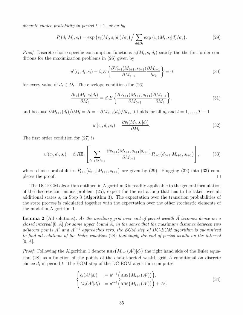
discrete choice probability in period t+ 1, given by

Pt(dt|Mt, st) = exp(vt(Mt, st|dt)/σε

)/∑d∈Dt

exp(vt(Mt, st|d)/σε

). (29)

Proof. Discrete choice specific consumption functions ct(Mt, st|dt) satisfy the the first order con-ditions for the maximization problems in (26) given by

u′(ct, dt, st) + βtE

{∂Vt+1(Mt+1, st+1)

∂Mt+1

∂Mt+1

∂ct

}= 0 (30)

for every value of dt ∈ Dt. The envelope conditions for (26)

∂vt(Mt, st|dt)∂Mt

= βtE

{∂Vt+1(Mt+1, st+1)

∂Mt+1

∂Mt+1

∂Mt

}, (31)

and because ∂Mt+1(dt)/∂Mt = R = −∂Mt+1(dt)

/∂ct, it holds for all dt and t = 1, . . . , T − 1

u′(ct, dt, st) =∂vt(Mt, st|dt)

∂Mt

. (32)

The first order condition for (27) is

u′(ct, dt, st) = βtREt

∑dt+1∈Dt+1

∂vt+1(Mt+1, st+1|dt+1)

∂Mt+1

Pt+1

(dt+1|Mt+1, st+1

) , (33)

where choice probabilities Pt+1

(dt+1|Mt+1, st+1

)are given by (29). Plugging (32) into (33) com-

pletes the proof.

The DC-EGM algorithm outlined in Algorithm 3 is readily applicable to the general formulationof the discrete-continuous problem (25), expect for the extra loop that has to be taken over alladditional states st in Step 3 (Algorithm 3). The expectation over the transition probabilities ofthe state process is calculated together with the expectation over the other stochastic elements ofthe model in Algorithm 1.

Lemma 2 (All solutions). As the auxiliary grid over end-of-period wealth A becomes dense on aclosed interval [0, A] for some upper bound A, in the sense that the maximum distance between twoadjacent points Aj and Aj+1 approaches zero, the EGM step of DC-EGM algorithm is guaranteedto find all solutions of the Euler equation (28) that imply the end-of-period wealth on the interval[0, A].

Proof. Following the Algorithm 1 denote rhs(Mt+1(A

j)|dt)the right hand side of the Euler equa-

tion (28) as a function of the points of the end-of-period wealth grid A conditional on discretechoice dt in period t. The EGM step of the DC-EGM algorithm computesct(A

j|dt) = u′−1(rhs

(Mt+1(A

j)))

,

Mt(Aj|dt) = u′−1

(rhs

(Mt+1(A

j)))

+ Aj.(34)

35

Both equations in (34) are well defined functions of Aj provided that the utility function u(·)satisfies the Assumption 1. Thus, the system constitutes a well defined parametric specification ofthe curve composed of the solutions to the Euler equation c(Mt, st|dt) for all st, dt, where Aj playsthe role of a parameter. In the limit as Aj runs through all the values on the interval [0, A], allsolutions that imply the end-of-period wealth from this interval are found.

The criteria for selecting the solutions of the Euler equation that correspond to the optimalbehavior in the model is based on the monotonicity of the savings function, which is establishedwith the following theorem19.

Theorem 3 (Monotinicity of savings function). Denote At(Mt, st|dt) = Mt−ct(Mt, st|dt) a discretechoice specific savings function in period t. Under the Assumption 1, function At(M, st|dt) ismonotone non-decreasing in M for all t,st and dt ∈ Dt.

Proof. Theorem 3 is an application of Theorem 4 in Milgrom and Shannon (1994) to the currentproblem. Conditional savings function At(Mt, st|dt) is a maximizer in the expression similar to(26) for the discrete choice specific value function vt(Mt, st|dt). As a function of M and A, themaximand in this expression is given by

f(A,M) = u(M − A, dt, st) + βtEt

{Vt+1(Mt+1(A), st+1)

}(35)

whereMt+1(A) is next period wealth as an increasing function of A. It is necessary and sufficient toshow that f(A,M) is quasisupermodular in A and satisfies the single crossing property in (A,M).The former is trivial because A is a scalar. For the latter consider A′ > A′′, M ′ > M ′′ and assumef(A′,M ′′) > f(A′′,M ′′). Then

f(A′,M ′)− f(A′′,M ′) =

= u (M ′ − A′, dt, st)− u (M ′ − A′′, dt, st)+

+βt [EVt+1 (Mt+1(A′), st+1)− EVt+1 (Mt+1(A

′′), st+1)] ≥≥ u (M ′′ − A′, dt, st)− u (M ′′ − A′′, dt, st)+

+βt (EVt+1 (Mt+1(A′), st+1)− EVt+1 (Mt+1(A

′′), st+1)) =

f(A′,M ′′)− f(A′′,M ′′) > 0.

(36)

For the first inequality we use

u (M ′ − A′, dt, st)− u (M ′ − A′′, dt, st) ≥ u (M ′′ − A′, dt, st)− u (M ′′ − A′′, dt, st) ,

u (M ′ − A′, dt, st)− u (M ′′ − A′, dt, st) ≥ u (M ′ − A′′, dt, st)− u (M ′′ − A′′, dt, st) ,

u (z, dt, st)− u (z −∆M , dt, st) ≥ u (z +∆A, dt, st)− u (z +∆A −∆M , dt, st) ,

(37)

where z = M ′ − A′, ∆A = A′ − A′′ > 0, ∆M = M ′ − M ′′ > 0, and which is due to Assumption1, i.e. concavity of the utility function. It follows then that f(A′,M ′) > f(A′′,M ′). Similarly,assumption f(A′,M ′′) ≥ f(A′′,M ′′) leads to f(A′,M ′) ≥ f(A′′,M ′), and thus f(A,M) satisfies thesingle crossing property, and monotonicity theorem in Milgrom and Shannon (1994) applies.

19A similar monotonicity result is also used in Fella (2014).

36

B Spurious Discontinuities from Numerical Integration

To illustrate how naive numerical quadrature integration can produce spurious discontinuities inthe policy function, we here focus on the illustrative model without smoothing. Particularly, forworking households, the smoothed Euler equation in (15) collapses to

u′ (ct (Mt|dt)) = β

∫ ∞

0

Ru′(ct+1(Mt+1|dt+1 = 1)) · 1{Mt+1 ≤ M t+1}f(dη)

+ β

∫ ∞

0

Ru′(ct+1(Mt+1|dt+1 = 0)) · 1{Mt+1 > M t+1}f(dη). (38)

where we recall that Mt+1 = R (Mt − ct (Mt|dt)) + yη. With the change of variables, q = f(η), wecan write the Euler equation (38) as

u′ (ct (Mt|dt)) = β

∫ qt

0

f−1(q)u′ (ct+1

(R(Mt − ct(Mt|dt)) + yf−1(q), dt+1 = 1

))dq

+ β

∫ 1

qt

f−1(q)u′ (ct+1

(R(Mt − ct(Mt|dt)) + yf−1(q), dt+1 = 0

))dq (39)

where the threshold qt is given by

qt = f

(M t+1

Mt+1

). (40)

As long as the income shock distribution is not degenerate, the resulting Euler equation (39) iscontinuous and smooth in ct(Mt,W) through Mt+1 in spite of the discontinuity in the consumptionfunction ct+1(Mt+1,W) at Mt+1 = M t+1. In turn, this suggests that numerical integration shouldbe done twice – once for each case – to ensure that the integral is well-behaved.

In contrast, the naive Euler equation in (38) is discontinuous in ct(Mt,W). When using nu-merical quadrature to evaluate the integral, for a given level of resources, some of the nodes willresult in Mt+1 ≤ M t+1 while others will result in the opposite case. For concreteness, say that 10nodes are used and the five lowest nodes results in Mt+1 ≤ M t+1. Say also that for a slightly largervalue of current resources perhaps only four nodes satisfy Mt+1 ≤ M t+1 while now six invokesthe alternative. When comparing the solution found in the two (close) values of current periodresources, there will be a discontinuous change in the optimal consumption. In the current model,this would result in spurious downward kinks in the consumption function around a secondarykink, as illustrated in the left panel of Figure 3.

C Derivation of the analytical solution to consumption re-

tirement problem

It is straightforward to show using backward induction that the value function for a retiree at ageT − t (i.e. t periods before end of life) is a logarithmic function of M20

vT−t(M |d = 0) = log(M)

(t∑

i=0

βi

)+ At (41)

20See Phelps (1962); Hakansson (1970).

37

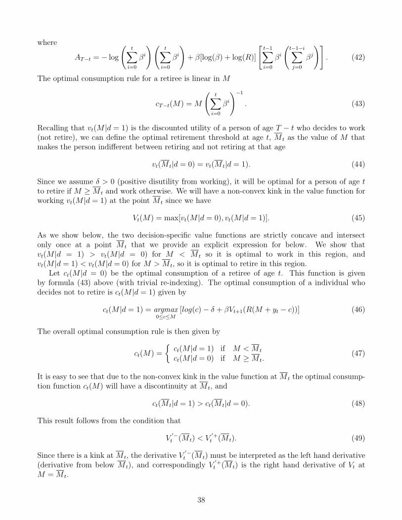
where

AT−t = − log

(t∑

i=0

βi

)(t∑

i=0

βi

)+ β[log(β) + log(R)]

[t−1∑i=0

βi

(t−1−i∑j=0

βj

)]. (42)

The optimal consumption rule for a retiree is linear in M

cT−t(M) = M

(t∑

i=0

βi

)−1

. (43)

Recalling that vt(M |d = 1) is the discounted utility of a person of age T − t who decides to work(not retire), we can define the optimal retirement threshold at age t, M t as the value of M thatmakes the person indifferent between retiring and not retiring at that age

vt(M t|d = 0) = vt(M t|d = 1). (44)

Since we assume δ > 0 (positive disutility from working), it will be optimal for a person of age tto retire if M ≥ M t and work otherwise. We will have a non-convex kink in the value function forworking vt(M |d = 1) at the point M t since we have

Vt(M) = max[vt(M |d = 0), vt(M |d = 1)]. (45)

As we show below, the two decision-specific value functions are strictly concave and intersectonly once at a point M t that we provide an explicit expression for below. We show thatvt(M |d = 1) > vt(M |d = 0) for M < M t so it is optimal to work in this region, andvt(M |d = 1) < vt(M |d = 0) for M > M t, so it is optimal to retire in this region.

Let ct(M |d = 0) be the optimal consumption of a retiree of age t. This function is givenby formula (43) above (with trivial re-indexing). The optimal consumption of a individual whodecides not to retire is ct(M |d = 1) given by

ct(M |d = 1) = argmax0≤c≤M

[log(c)− δ + βVt+1(R(M + yt − c))] (46)

The overall optimal consumption rule is then given by

ct(M) =

{ct(M |d = 1) if M < M t

ct(M |d = 0) if M ≥ M t.(47)

It is easy to see that due to the non-convex kink in the value function at M t the optimal consump-tion function ct(M) will have a discontinuity at M t, and

ct(M t|d = 1) > ct(M t|d = 0). (48)

This result follows from the condition that

V′−t (M t) < V

′+t (M t). (49)

Since there is a kink at M t, the derivative V′−t (M t) must be interpreted as the left hand derivative

(derivative from below M t), and correspondingly V′+t (M t) is the right hand derivative of Vt at

M = M t.

38

We now establish these results by backward induction, starting at period T−1 which is the firstperiod where the consumption/retirement decision is non-trivial (it is easy to see that in the finalperiod of life, it is optimal to retire and consume all remaining savings). For notational simplicity,we drop the time subscripts on income, y = yt, since income is constant here. To derive a formulafor the retirement threshold MT−1 consider the T − 1 optimization problem

cT−1(M |d = 1) = argmax0≤c≤M

[log(c)− δ + β log(R(M − c) + y)] . (50)

The solution to this is given by

cT−1(M |d = 1) =

{M if M < y/Rβ(M + y/R)/(1 + β) if y/Rβ ≤ M ≤ MT−1

(51)

Note that the worker is liquidity constrained when M < y/Rβ and in this region it is optimal toconsume all of her beginning of period savings M and rely on the end of period payment of wageearnings y to finance consumption in her last period of life, T . The value function for the workerat age T − 1 is

vT−1(M |d = 1) ={log(M)− δ + β log(y) if M < y/Rβlog(M + y/R)(1 + β)− δ + β[log(β) + log(R)]− log(1 + β)(1 + β) if y/Rβ ≤ M ≤ MT−1

and the value function for a retiree is given by equation (41). Equating the values of work andretirement and solving for the optimal retirement threshold MT−1 we have

MT−1 =(y/R) exp{−δ/(1 + β)}1− exp{−δ/(1 + β)}

(52)

provided this is greater than y/Rβ (the threshold below which the consumer is liquidity con-strained), otherwise

MT−1 = [y/(Rβ)](1 + β)(1+β)

β exp{−δ/β}. (53)

However it is easy to see that assumption δ < (1 + β) log(1 + β) implies that MT−1 > y/Rβ. It isalso easy to see that as the disutility of working δ → ∞ we have MT−1 → 0, and as δ → 0, thenMT−1 → ∞, i.e. if there is no disutility of working, the person would never choose to retire.

Note also that at MT−1 there is a kink in the value function: this is a downward kink (interms of Clausen and Strub (2013)) as the max of two concave functions vT−1(M |d = 0) andvT−1(M |d = 1), and this kink in the value function results in a discontinuity in the optimalconsumption function cT−1(M). There is a drop in consumption equal to (y/R)/(1 + β) at MT−1,and with two remaining periods in their life, a retiree has a “marginal propensity to consume” outof wealth equal to 1/(1 + β) the same as a worker. The discontinuous drop in consumption thatoccurs at the retirement threshold equals the present value of forgone earnings due to retirement,yT−1/R, multiplied by the marginal propensity to consume out of wealth, 1/(1 + β).

To summarize the solution at T−1, the optimal retirement threshold is MT−1 given in equation

39

(52) and the consumption function is given by

cT−1(M) =

M if M < y/Rβ(M + y/R)/(1 + β) if y/Rβ ≤ M ≤ MT−1

M/(1 + β) if M > MT−1

(54)

and the value function is given by

VT−1(M) = (55)log(M)− δ + β log(y) if M < y/Rβlog(M + y/R)(1 + β)− δ + β[log(β) + log(R)]− log(1 + β)(1 + β) if y/Rβ ≤ M ≤ MT−1

log(M)(1 + β) + β[log(β) + log(R)]− log(1 + β)(1 + β) if M > MT−1.

Now consider going back one more time period in the backward recursion, to T − 2. We wantto illustrate the possibility of secondary kinks/discontinuities in the consumption function for aworker cT−2(M, 1) caused by the kinks in VT−1(M). Let MT−2 denote the primary kink due to theretirement threshold at T − 2 and let M

rjT−2 denote the secondary kinks, where j = 1, . . . , NT−2

and NT−t is the number of secondary kinks t periods before the end of life at age T .To see how these secondary kinks arise, consider how the T − 2 consumption function is deter-

mined, as the solution to

cT−2(M, 1) = argmax0≤c≤M

[log(c)− δ + βVT−1(R(M − c) + y)] . (56)

As shown above VT−1(M) has two kinks: one at M = y/Rβ where the liquidity constraint stopsbeing binding, and the other at MT−1 where the worker retires. Assume that the initial wealthof the worker at the start of period T − 1 is low enough so that the worker will be liquidityconstrained in period T − 1. This implies that R(M − c) + y < y/Rβ. Then substituting theliquidity-constrained formula for VT−1(M) from (55) into the period T − 2 optimization (56), wefind that optimal consumption is given by ct−2(M, 1) = (M +y/R)/(1+β). However imposing theliquidity constraint, we must also have (M+y/R)/(1+β) ≤ M which implies that M ≤ y/Rβ, andit is easy to verify that for wealth satisfying this constraint, the worker will be liquidity constrainedboth in period T − 2 and in period T − 1 as well.

However for wealth above y/Rβ the worker is no longer liquidity constrained in period T−2 butour derivation of the worker’s consumption in period T − 2 is still contingent on the assumptionthat the worker is liquidity constrained in period T − 1. This will be true provided that thesavings and earnings the worker brings to the start of period T − 1, Rβ(M + y/R)/(1 + β), isless than y/Rβ, which is equivalent to the inequality M ≤ [y/(Rβ)2](1 + β − Rβ2). It is nothard to show that when R = 1 we have y/β < (y/β2)(1 + β − β2) so the interval for whichthe consumer will consume (M + y)/(1 + β) is non-empty when R = 1. For R > 1 the inequalityy/(Rβ) < [y/(Rβ)2](1+β−Rβ2) is equivalent to Rβ < 1, so under this assumption this interval willalso exist, otherwise the interval is empty and the consumer goes from consuming cT−2(M, 1) = Mto consuming an amount we derive below.

In the next region, wealth is sufficiently high in period T − 2 so the consumer is not liquidityconstrained at T − 2 and the saving and earning will keep the consumer out of the liquidityconstrained region at T − 1, but the worker’s wealth is not high enough to retire at T − 1. Therelevant expression for VT−1(M) in this case is given by the middle expression in equation (55).This implies an optimal consumption level equal to cT−2(M, 1) = (M+y(1/R+1/R2))/(1+β+β2).

40

For even larger there will come a point where the consumer can save enough in period T − 2to retire in period T − 1, i.e. savings will exceed the MT−1 threshold. Thus, there is some wealthlevel M

r

T−2 at which the the relevant expression for the worker’s period T − 1 value functionVT−1(M) is given by the last, retirement, formula in (55). The optimal consumption in thisregion is cT−2(M, 1) = (M + y/R)/(1 + β + β2). It is important to carefully check values of csuch that savings, M + y − c is in the “convex region” of VT−1(M) around the T − 1 retirementthreshold MT−1. In this region there will be two local optima for c, one involving the higherconsumption (M + y(1/R + 1/R2))/(1 + β + β2) and the other involving the lower consumption(M + y/R)/(1 + β + β2) that enables the worker to retire at T − 1.

These two solutions are reflected in the two possible solutions to the first order condition foroptimal consumption given by

0 =1

c−{

(β + β2)/(M − c+ y(1/R + 1/R2)) if R(M − c) + y < MT−1

(β + β2)/(M − c+ y/R) if R(M − c) + y ≥ MT−1(57)

For M < Mr

T−2 the global optimum will be cT−2(M, 1) = (M + y(1/R + 1/R2))/(1 + β + β2)

and the consumer will be working in both periods T − 2 and T − 1. However for M > Mr

T−2 theconsumer will still work at T−2 (provided M < MT−2, the primary kink point at T−2, the wealththreshold at which the consumer retires at T − 2) but will have enough savings to retire at T − 1.The optimal consumption in this case will be cT−2(M, 1) = (M + y/R)/(1+β+β2). It is not hardto show that if M ≤ [y/(Rβ)2](1+β−Rβ2), then the quantity R(M−cT−2(M, 1))+y ≤ y/Rβ, i.e.the consumer will indeed be in the liquidity constrained region M ≤ y/Rβ at the start of T − 1 aswe assumed would be the case. We also have that y/Rβ < [y/(Rβ)2](1 + β − Rβ2) provided thatRβ ≤ 1, which we assume to be the case. Otherwise this region would be empty and the optimalconsumption would be given by cT−2(M, 1) = (M + y(1/R+1/R2))/(1+β+β2) as derived above.We can check that this consumption function, which is also derived under the assumption that theconsumer will not be liquidity constrained at period T − 1, will result in total savings at T − 1that satisfies R(M − c) + y ≥ y/Rβ (so the consumer is not liquidity constrained at T − 1) forwealth at T − 2 at the lower end of this interval (i.e. at M = y/Rβ) provided that R ≤ 1/β.

However, at M = Mr

T−2 the consumer will be indifferent between consuming the larger amount(M + y(1/R+1/R2))/(1+β+β2) knowing they will not retire at T − 1 and consuming the loweramount (M + y/R)/(1 + β + β2) and knowing they will retire at T − 1. We find M

r

T−2 as thesolution to the following equation

log((M + y(1/R + 1/R2))/(1 + β + β2)

)+

βVT−1

((y +R(M − (M + y(1/R + 1/R2)))/(1 + β + β2))

)= log

((M + y/R)/(1 + β + β2)

)+ βVT−1

(y +R(M − (M + y/R))/(1 + β + β2)

).

Thus, at M = Mr

T−2 the consumer is indifferent between consuming the larger amount(M + y(1/R+1/R2))/(1+β+β2) or consuming the smaller amount (M + y/R)/(1+β+β2) thatprovides the additional savings necessary to enable the consumer to retire at T − 1.

Now we can express period T − 2 consumption of the worker as the following piece-wise linear

41

function:

cT−2(M, 1) =

M if M < y/Rβ(M + y/R)/(1 + β) if y/Rβ ≤ M ≤ [y/(Rβ)2](1 + β −Rβ2)

(M + y(1/R + 1/R2))/(1 + β + β2) if [y/(Rβ)2](1 + β −Rβ2) ≤ M ≤ Mr

T−2

(M + y/R)/(1 + β + β2) if Mr

T−2 < M < MT−2.(58)

It is straightforward to verify that cT−2(M, 1) has two kinks at M = [y/(Rβ)2](1 + β − Rβ2) andM = y/Rβ followed by a discontinuity at M = M

r

T−2.To derive the time T − 2 retirement threshold MT−2 we solve for the value of M that

makes the consumer indifferent between retiring at T − 2 and working (but with enough wealthso that the person is above the secondary kink M

r

T−2 where their consumption is given bycT−2(M, 1) = (M + y/R)/(1 + β + β2))

log(M)(1 + β + β2) + AT−2 = log(M + y/R)(1 + β + β2)− δ + AT−2 (59)

where AT−2 is defined in equation (42) above. Note that the right hand side of (59) is the valuefunction for a consumer who does not have enough wealth to retire at T − 2, but since M > M

r

T−2

(the secondary kink point), it follows that the appropriate formula for VT−1(M) will be the onewhere M > MT−1 in equation (55) above. The solution to this equation is MT−2 given by

MT−2 =(y/R)e−K

(1− e−K)(60)

where K is given by

K =δ

(1 + β + β2). (61)

Notice that formulas (60) and (52) imply that MT−1 < MT−2, i.e. the wealth threshold forretirement decreases as one approaches the end of life, T .

To summarize the solution we found at T − 2, the optimal retirement threshold MT−2 is thesolution to equation (59), and the optimal consumption function is given by

cT−2(M) =

M if M < y/Rβ(M + y/R)/(1 + β) if y/Rβ ≤ M ≤ [y/(Rβ)2](1 + β −Rβ2)

(M + y(1/R + 1/R2))/(1 + β + β2) if [y/(Rβ)2](1 + β −Rβ2) ≤ M ≤ Mr

T−2

(M + y/R)/(1 + β + β2) if Mr

T−2 < M ≤ MT−2

M/(1 + β + β2) if M > MT−2.(62)

The optimal consumption function at T − 2 has two kinks at M = y/Rβ (the level of wealthat which the consumer is no longer liquidity-constrained) and M = [y/(Rβ)2](1 + β − Rβ2),and two discontinuities: one at the secondary kink point M

r

T−2 where consumption drops by(y/R2)/(1 + β + β2), and the other at the retirement threshold MT−2 where consumption dropsby another (y/R)/(1+ β + β2). Note that the secondary kink point M

r

T−2 is precisely the amountof wealth where, while the consumer does not yet retire at T − 2, they know they will have enoughto retire at T − 1. Thus, the drop in consumption at this secondary kink point can be regarded assaving at T − 2 for their anticipated retirement at time T − 1.

42

The value function at T − 2 can be expressed this way:

VT−2(M) =

{log(cT−2(M))− δ + βVT−1(R(M − cT−2(M)) + y) if M < MT−2

log(M)(1 + β + β2) + AT−2 if M ≥ MT−2(63)

Thus, depending on whether the person’s wealth at T − 2 is above or below the secondary kinkpoint M

r

T−2, they will know whether they will have enough (with their T − 2 earnings y) to retireat T − 1 or not, and will save/consume accordingly.

Now consider solving the problem at t = T − 3, three periods before the end of life. Theconsumption rule will have three kinks including the level of M where the liquidity constraint nolonger binds, and three discontinuities, including the retirement threshold M

r

T−3 in period T − 3.One additional kink in cT−3(M) is added above the end point [y/(Rβ)2](1 + β −Rβ2) of the firstlinear segment of cT−2(M) and reflects to the liquidity constraint in period T − 2. The additionaldiscontinuity corresponds to the secondary kink point M

r

T−2.Note the pattern here: cT−1(M) has one kink and one discontinuity, cT−2(M) has two kinks and

two discontinuities, and cT−3(M) will have three kinks and three discontinuities. The importantadditional point to notice is that cT−1, cT−2 and as we show shortly, cT−3, are all piecewise linear.

It will be helpful to distinguish the points marking the sequence of connected linear segments ofthe consumption function due to kinks in the value function arising at the end of the liquidity con-strained region [0, y/Rβ] from those at higher levels of wealth that related to retirement decisions— both current retirement and anticipated future retirements. As we noted the will always be aninitial linear segment over the interval [0, y/Rβ] where ct(M) = M for M ∈ [0, y/Rβ]. Thus therewill be a kink in the consumption function at y/Rβ related to current period liquidity constraint.We have also shown that for M > M t it will be optimal to retire, so there is a discontinuity inct(M) at M t which relates to the primary kink in the value function and the decision to retire inthe current period.

However at ages T − t < T − 1 in addition to these two “current period” kinks/discontinuities,there will be a set of kinks and discontinuities related to the future periods, i.e. “future liquidity

constraint” kinks MljT−t and a set of “future retirement threshold” discontinuities M

rjT−t. These

discontinuities correspond to secondary kinks in the same period value function and result fromthe primary kinks in the value functions of all future periods.

Thus cT−2(M) has one future liquidity constraint kink Ml1T−2 at [y/(Rβ)2](1 + β − Rβ2) and

one future retirement threshold discontinuity at Mr1T−2. The former represents the level of saving

at which the consumer is not liquidity constrained at age T − 2, but will be liquidity constrainedat age T − 1. The latter is the level of wealth that leads the worker to discontinuously reduceconsumption at T − 2 in order to have enough savings to retire at T − 1.

In period T − 3 there will be a total of tree discontinuities in cT−3(M). The last discontinuityoccurs at the retirement threshold MT−3, but there will be two additional discontinuities at thesecondary kink points in the value function VT−3. These are denoted M

r1T−3 and M

r2T−3. We have

the ordering MT−3 > Mr1T−3 > M

r2T−3. The highest secondary kink point M

r1T−3 is the level of

wealth that leads the consumer to save an amount (including current period wage earnings) ofMT−2, which is the retirement threshold at period T − 2. Thus at wealth levels that just exceedM

r1T−3 the consumer works in period T − 3 but discontinuously reduces consumption in order to

have enough resources to retire in period T − 2. At wealth levels that are just below Mr2T−3, the

consumer works in both periods T − 3 and T − 2, and retires only in period T − 1.The consumption function cT−3(M) will also have two future liquidity constraint kinks

43

Ml1T−3 = [y/(Rβ)2](1 + β − Rβ2) and M

l2T−3 in addition to the current liquidity constraint

at M = y/Rβ. The first kink will be at the level of saving that is sufficient for the con-sumer not to be liquidity-constrained at age T − 3 but not enough to avoid being liquidity

constrained at age T − 2. At Ml1T−3 the consumer switches from consuming according to the

2nd linear segment of cT−3(M) = (M + y/R)/(1 + β) to consuming on the third linear segmentcT−3(M) = (M + y(1/R + 1/R2))/(1 + β + β2).

At the second future liquidity constraint kink point Ml2T−3 the worker has sufficient saving to

not be liquidity constrained at both ages T − 3 and T − 2, but not enough to avoid being liquidity

constrained at age T − 1. At Ml2T−3 the worker switches from consuming on the third segment

of cT−3(M) = (M + y(1/R + 1/R2))/(1 + β + β2) to the fourth segment which is the first ofthe segments created by the retirement threshold kink points M

rjT−3. Thus for wealth that exceeds

Ml2T−3 consumption switches to cT−3(M) = (M+y(1/R+1/R2+1/R3))/(1+β+β2+β3). Then for

still higher levels of wealth the worker consumes according to the various piecewise linear segmentsdemarcated by the successive future retirement threshold kink points M

rjT−3, j = 2, 1 and finally

MT−3, the retirement threshold at period T − 3.Note that the marginal propensity to consume out of wealth is also piecewise linear and mono-

tonically decreasing in M . In the liquidity constrained region the marginal propensity to consumeis 1, and in the first of the liquidity constrained consumption segments it is 1/(1 + β), and in thesecond liquidity constrained segment it is 1/(1+β+β2). Then in the remaining retirement relatedconsumption segments, the marginal propensity to consume out of wealth is constant and equalto 1/(1 + β + β2 + β3).

In summary, the consumption function cT−3(M) is given by

cT−3(M) =

M if M < y/Rβ

(M + y/R)/(1 + β) if y/Rβ ≤ M ≤ Ml1T−3

(M + y(1/R + 1/R2))/(1 + β + β2) if Ml1T−3 ≤ M ≤ M

l2T−3

(M + y(1/R + 1/R2 + 1/R3))/(1 + β + β2 + β3) if Ml2T−3 ≤ M ≤ M

r2T−3

(M + y(1/R + 1/R2))/(1 + β + β2 + β3) if Mr2T−3 ≤ M < M

r1T−3

(M + y/R)/(1 + β + β2 + β3) if Mr1T−3 ≤ M < MT−3

M/(1 + β + β2 + β3) if MT−3 < M

(64)

The retirement threshold MT−3 is given by

MT−3 =(y/R)e−K

(1− e−K), where K =

δ

(1 + β + β2 + β3). (65)

We solve for the secondary kinks/discontinuities {M liT−3,M

rjT−3}, i = 1, 2 and j = 1, 2 in the same

way as we did for the period T − 2: we solve for the level of a wealth that makes the consumerindifferent between consuming the higher level of consumption to the “left” of the kink point(more precisely the limit of consumption for wealth approaching the kink point from below) andthe lower level of consumption to the “right” of the discontinuity (the limit of consumption forwealth approaching the kink point from above).

Finally, the value function is given by

VT−3(M) =

{log(cT−3(M))− δ + βVT−2(R(M − cT−3(M)) + y) if M < MT−3

log(M)(1 + β + β2 + β3) + AT−3 if M ≥ MT−3(66)

44

Due to the monotonicity of the saving function, the fact that MT−2 > Mr

T−2 implies that

Ml1T−3 > M l2

T−3 > Mr1T−3 > M

r2T−3. Similarly, it is not hard to show that MT−3 > MT−2.

Having solved for the consumption function explicitly by doing backward induction for 3 peri-ods, it is easy to see the general pattern. At t periods before the end of life T , t ≥ 1, i.e. at periodT − t, the consumption function cT−t(M) will have a total of t kinks relating to current and future

liquidity constraints, namely y/Rβ and MljT−t, j = 1, . . . , t−1; t−1 discontinuities relating the the

future retirement thresholds denoted MrjT−t, j = 1, . . . , t − 1, and one discontinuity at the period

t retirement threshold MT−t. Consequently, cT−t(M) will have 2t + 1 linear segments. For everyperiod T − t, t ≥ 1 there will be a kink in the consumption function at M = y/Rβ correspondingto the end of the liquidity constrained region, [0, y/Rβ].

Under the assumptions Rβ ≤ 1 and δ < (1 + β) log(1 + β) all the kink/discontinuity pointsdefine non-empty intervals such that the following ordering holds

y/Rβ < Ml1T−t < M

l2T−t < · · · < M

lt−1

T−t < Mrt−1

T−t < Mrt−2

T−t < · · · < Mr2T−t < M

r1T−t < MT−t. (67)

The first of the future liquidity constraint kink points is always at the same value of M ,

Ml1T−t = [y/(Rβ)2](1 + β −Rβ2) for t ≥ 2. (68)

Period T − t retirement threshold MT−t is given by

MT−t =(y/R)e−K

(1− e−K), where K = δ

(t∑

i=0

βi

)−1

. (69)

The values of the last t − 2 future liquidity constraint kink points MljT−t, j = 2, . . . , t − 1 and

the future retirement threshold discontinuity points MrjT−t, j = 1, . . . , t− 2 are determined by the

values of wealth that make the consumer indifferent between consuming according to the linearsegments of the consumption function on either side of each of these kink points as describedabove.

The value function VT−t(M) can be expressed recursively in terms of the already defined valuefunction VT−t+1(M) one period ahead:

VT−t(M) =

{log(cT−t(M))− δ + βVT−t+1(R(M − cT−t(M)) + y) if M < MT−t

log(M)(∑t

i=0 βi)+ AT−t if M ≥ MT−t

(70)

where AT−t was defined in equation (42) above. It is then straightforward to show with the formalmathematical induction argument the general formula (7).

D DC-EGM run times

Figure 10 illustrates the average estimation time spent to estimate δ. Results are shown forvarying degree of income uncertainty, ση ∈ {0.001, 0.05}, and different values of the disutility ofwork parameter, δ ∈ {0.1, 0.5}

45

Figure 10: Timing: income uncertainty.

(a) σ2η = 0.001

0 100 200 300 400 5000

10

20

30

40

50

60

# of gridpoints

Est

imat

ion

time

(sec

s)

σε = 0.01σε = 0.05

(b) σ2η = 0.05

0 100 200 300 400 5000

10

20

30

40

50

# of gridpoints

Est

imat

ion

time

(sec

s)

σε = 0.01σε = 0.05

Notes: The plots illustrate the time spent to estimate the model. Results are shown for varying degree of smoothing,

σε ∈ {0.01, 0.05}, and different values of the income variance, σ2η ∈ {0.001, 0.05}. The rest of parameters are at

their baseline levels, see Table 1.

E Proof of Extreme Value Homotopy Principle

This appendix proves Theorem 2 which states that the value function and optimal decision rulesin the presence of Type I extreme value distributed taste shocks converge (in an appropriatesense to be defined below) to the value functions and decision rules of a limiting problem withouttaste shocks. We prove Theorem 2 for a more general class of problems than just the retirementconsumption model, and therefore restate it below.

Let ε be a random variable having a standardized Type I extreme value distribution with CDFF (ε) given by

F (ε) = exp{− exp{−ε}}. (71)

We have E{ε} = γ, where γ = 0.577 . . . is Euler’s constant and var(ε) = π2/6. Then if σ is apositive scaling constant, σε will also be a Type I extreme value distribution with expected valueσγ and variance σ2π2/6. In the notation of the illustrative model in the paper, σ corresponds tothe scaling parameter of the “perturbed” model σε.

The homotopy convergence result we prove below holds for a considerably more general class ofdynamic programming problems than the simple retirement example we analyzed in section 2.1 oreven the class defined in Appendix A, where we assumed the continuous choice is a unidimensionalvariable and we imposed additional assumptions to ensure monotonicity of the savings function. Inthis appendix we consider a more general class of problems, though we do not strive for maximumpossible generality in order to make our proof as straightforward as possible.

Consider a finite horizon DP problem without Type I extreme value taste shocks which we alsorefer to as the “unperturbed” DP problem. In the last period, T , the agent chooses a vector ofk continuous choice variables c ∈ CT (d, s), where CT (d, s) is a compact subset of a Rk and d isone of the discrete choices and s is a potentially multidimensional vector of state variables in someBorel subset S of a finite dimensional Euclidean space. We assume that the discrete choice d is anelement of a finite choice set DT (s). Let uT (d, c, s) be a utility function that is continuous in c for

46

each s and each d ∈ DT (s) and a Borel measurable function of s for each c and d. Then the valuefunction in period T is VT (s) given by

VT (s) = maxd∈DT (s)

maxc∈CT (d,s)

uT (d, c, s). (72)

Now consider time T − 1 and let pT (s′|s, c, d) be a Markov transition probability providing the

conditional probability distribution over the state s′ at time T given that the state vector at timeT−1 is s, the discrete choice is d, and the continuous choice is c. Define the conditional expectationof VT , EVT−1(d, c, s), by

EVT−1(d, c, s) =

∫VT (s

′)pT (∂s′|d, c, s) (73)

where we use ∂s′ to indicate the stochastic next period state variables over which this expectationis taken. In Assumption C below, we assume that this conditional expectation exists and iscontinuous in c for each s ∈ S and d ∈ DT−1(s). Then by backward induction we can define thevalue function VT−1(s) and, continuing for each t ∈ {T−1, T−2, . . . , 0} we can define the sequenceof functions {Vt} recursively using Bellman’s equation

Vt(s) = maxd∈Dt(s)

maxc∈Ct(d,s)

[ut(d, c, s) + β

∫Vt+1(s

′)pt+1(∂s′|d, c, s)

]. (74)

where β ≥ 0 is the agent’s discount factor.We make the following assumptions on this limiting DP problem without taste shocks that is

sufficient to guarantee the existence of a well defined solution.Assumption B The choice sets Dt(s) are all finite with a uniformly bounded number of elementsD given by

D = maxt∈{0,1,...,T}

sups∈S

|Dt(s)| < ∞ (75)

where |Dt(s)| denotes the number of elements in the finite set Dt(s).Assumption C For each t ∈ {0, 1, . . . , T} and each s ∈ S and each d ∈ Dt(s) the functionut(d, c, s) is continuous in c, and for each t ∈ {1, 2, . . . , T −1}, s ∈ S and d ∈ Dt−1(s) the functionEVt(d, c, s) is given by

EVt(d, c, s) =

∫Vt(s

′)pt(∂s′|d, c, s) (76)

is finite and continuous in c.Define the discrete choice-specific continuous choice function ct(d, s) by

ct(d, s) = argmaxc∈Ct(d,s)

[ut(d, c, s) + βEVt+1(d, c, s)] (77)

and the optimal discrete decision rule δt(s) by

δt(s) = argmaxd∈Dt(s)

[ut(d, ct(d, s), s) + βEVt+1(d, ct(d, s), s)] . (78)

The overall optimal continuous decision rule ct(s) is then given by

ct(s) = ct(δt(s), s). (79)

47

The solution to the DP problem is given by the collection Γ of the T + 1 value functions{V0, V1, . . . , VT}, the T + 1 optimal continuous decision rules {c0, c1, . . . , cT} and the T + 1 op-timal discrete decision rules {δ0, δ1, . . . , δT}.

Now we define a family of perturbed DP problems index by σ, the scale parameter of the Type IExtreme value distribution. Let ε denote a vector of IID extreme value random variables withthe same dimension as |Dt(s)|, the number of elements in the finite choice set Dt(s). Assumethe elements of DT (s) are ordered in some fashion and let ε(d) be the component of the vector εcorresponding to the choice of alternative d ∈ Dt(s). We will refer to ε(d) as the “dth taste shock”.

Now consider the last period T . The value function Vσ,T (s, ε) is given by

Vσ,T (s, ε) = maxd∈DT (s)

maxc∈CT (d,s)

[uT (d, c, s) + σε(d)] . (80)

Notice that Vσ,T is now a function of the vector s and the vector ε ∈ R|DT (s)|. If the number ofelements of DT (s) varies with s ∈ S we can embed the vector ε in RD where D is the upper boundon the number of discrete choices by Assumption. We can use the convention that if |DT (s)| < Dfor some s ∈ S, the function Vσ,T (s, ε) depends only on the components of ε corresponding to thefeasible choices d ∈ DT (s) and not on any components d that are not elements of DT (s).

The CDF F (ε) of the vector random variable ε is given by the product of the univariate Type IExtreme value CDFs, i.e.

F (ε1, . . . , εD) =D∏

d=1

exp{− exp{−ε(d)}} (81)

To compute the expected value of VT (s, ε) we apply multivariate integration to get

EVσ,T (d, c, s) =

∫s′

∫ε′Vt(s

′, ε′)F (∂ε′)pT (∂s′|d, c, s)

=

∫s′σ log

∑d∈DT (s′)

exp{uT (d, cT (s, d), d)/σ}

pT (∂s′|d, c, s) (82)

where cT (s, d) = argmax c∈CT (d,s) uT (d, c, s) is the choice-specific continuous choice function. Theclosed form expression for the expectation over ε′ the Type I extreme value random variables isa consequence of a property of extreme value random variables known as max-stability i.e. themaximum of a finite collection of Type I extreme value random variables has a (shifted) Type Iextreme value distribution. We refer to the log-sum formula inside the integral of the lowerequation of (82) as the smoothed max function. We now prove a key Lemma that establishes abound between the usual max function and the smoothed max function.

Lemma 3 (Logsum error bounds). Let {v1, . . . , vD} be any finite set of D real numbers and letσ > 0 be a constant. Then we have

0 ≤ σ log

(D∑

d=1

exp{vd/σ}

)−max{v1, . . . , vD} ≤ σ log(D). (83)

48

Proof. Consider the shifted values vd −max(v1, . . . , vD) ≤ 0. It follows that

log

(D∑

d=1

exp{(vd −max{v1, . . . , vD})/σ}

)≤ log

(D∑

d=1

exp{0}

)= log(D). (84)

Define d∗ = argmaxd(vd) and let J ≥ 1 denote the number of elements of D for which vd = vd∗ .The lower bound is obtained from observing that

log

(J +

D∑d=1,d =d∗

exp{(vd −max{v1, . . . , vD})/σ}

)≥ 0. (85)

Combining (84) and (85) with the identity

σ log

(D∑

d=1

exp{(vd −max{v1, . . . , vD})/σ}

)= σ log

(D∑

d=1

exp{vd/σ}

)−max{v1, . . . , vD} (86)

concludes the proof.

Lemma 3 is the key to all of our subsequent results and the key to Theorem 2 since it shows thatthe difference between the max function and the smoothed max function is bounded by σ log(D)and this tends to 0 as σ ↓ 0. This will imply that the difference between the value functions anddecision rules of the unperturbed limiting DP problem and the family of perturbed DP problemswith extreme value distributed taste shocks will converge to zero as the scale of the extreme valuetaste shocks, σ converges to 0.

We can now define the value functions at all time periods for the perturbed problem as thesequence {Vσ,0, . . . , Vσ,T} where Vσ,T is given by equation (80) and the other value functions aregiven by the Bellman recursion

Vσ,t(s, ε) = maxd∈Dt(s)

maxc∈Ct(d,s)

[ut(d, c, s) + σε(d) + βEVt+1(d, c, s)] (87)

where EVσ,t+1(d, c, s) is the conditional expectation of Vσ,t+1(s, ε) and is given by

EVσ,t+1(d, c, s) = σ

∫s′log

∑d′∈Dt+1(s′)

exp{vσ,t+1(d′, cσ,t+1(d

′, s′), s′)/σ}

pt+1(∂s′|d, c, s), (88)

wherevσ,t+1(d, c, s) = ut+1(d, c, s) + βEVσ,t+2(d, c, s) (89)

and cσ,t+1(d, s) is the choice-specific continuous choice rule given by

cσ,t+1(d, s) = argmaxc∈Ct+1(d,s)

[vσ,t+1(d, c, s)] . (90)

Note that we used the Williams-Daly-Zachary Theorem again to obtain the expression forEVt+1(d, c, s) in equation (88) and we also note that due to the assumption that taste shocksare not only contemporaneously independent across different discrete choices d but also intertem-porally independent processes, it follows that the value of the ε state vector at time t does not

49

affect the conditional expectation of Vσ,t+1, and hence does not enter the conditional expectationEVt+1(d, c, s). This conditional independence restriction on the ε shocks is critical to all resultsthat follow below.

Having defined the set of value functions for the family of perturbed problems we can definethe full solution of the perturbed problem as the collection Γσ consisting of the value functions(Vσ,0, . . . , Vσ,T ), the continuous decision rules (cσ,0, . . . , cσ,T ) and the the discrete decision rules(δσ,0, . . . , δσ,T ). Note that all of these objects depend on both s and ε, which constitute the fullvector of state variables in the perturbed problem. In particular, the discrete decision rule δσ,t(s, ε)can be defined using the choice-specific continuous choice rule cσ,t(d, s) as

δσ,t(s, ε) = argmaxd∈Dt(s)

[vσ,t(d, cσ,t(d, s), s) + σε(d)] , (91)

and the unconditional or continuous decision rule can be defined using the choice-specific contin-uous choice rules by

cσ,t(s, ε) = cσ,t(δσ,t(s, ε), s). (92)

To define a notion of convergence of the solution Γσ of the family of perturbed DP problemsto the solution Γ of the limiting un-perturbed problem, we have to confront the difficulty that thestate space for the family of perturbed problems is the set of points of the form (s, ε) for s ∈ Sand ε ∈ RD whereas the state space of the limiting unperturbed problem is just S. We start bynoting the following representation for the value functions of the perturbed problem

Vσ,t(s, ε) = maxd∈Dt(s)

[vσ,t(d, cσ,t(d, s), s) + σε(d)] , (93)

which follows directly from the Bellman equation (87) and the definition of the vt function inequation (89). We now compute a partial expectation of the value functions Vσ,t(s, ε) over the εholding the s state variable fixed. That is we define the partial expectation EVσ,t(s) as the functiongiven by

EVσ,t(s) =

∫ε

Vσ,t(s, ε)F (ε)

= σ

∑d∈Dt(s)

exp{vσ,t(d, cσ,t(d, s), s)/σ}

. (94)

We are in the position now to state the main result which is a reformulation of Theorem 2 for amore general class of DC models than the consumption retirement model in Section 2.

Theorem 2 (Extreme Value Homotopy Principle). Under assumptions B and C above, let

Γ = {(V0, . . . , VT ), (δ0, . . . , δT ), (c0, . . . , cT )} (95)

be the solution to the limiting DP problem without taste shocks given in equations (72), (74), (77)and (78) above. Similarly, let

Γσ = {(Vσ,0, . . . , Vσ,T ), (δσ,0, . . . , δσ,T ), (cσ,0, . . . , cσ,T )} (96)

be the solution to the the perturbed DP problem with Type I extreme value taste shocks with scale

50

parameter σ > 0 given in equations (80), (87), (88), (91) and (92). Then as σ → 0 we have

limσ↓0

Γσ = Γ, (97)

where the convergence of value functions is defined in terms of the partial expectations of the valuefunctions for the perturbed problems with taste shocks, EVσ,t(s) given in equation (94) so that wehave uniform bound

∀t sups∈S

|EVσ,t(s)− Vt(s)| ≤ σ

[T−t∑j=0

βj

]log(D), (98)

and the decision rules converge pointwise for all (s, ε), s ∈ S and ε ∈ RD, i.e.

limσ↓0

δσ,t(s, ε) = δt(s)

limσ↓0

cσ,t(s, ε) = ct(s), (99)

assuming that the decision rules of the limiting problem δt(s), ct(s) are singletons, otherwise thelimits are elements of the sets (δt(s), ct(s)).

Proof. We prove Theorem 2 in three steps. First, we prove (98) by induction using Lemma 3 andshowing that the bounds are independent of s. Second, we prove convergence of decision rulesassuming that the limiting problem Γ has unique solution. Third, we extend the latter result tonon-singleton solution sets.

Lemma 4 (DP error bounds). Let Vt(s) be the value function for the unperturbed DP problem andlet EVσ,t(s) be the partial expectation of the value function Vσ,t(s, ε) to the perturbed DP problem.Then we have

∀t, s 0 ≤ EVσ,t(s)− Vt(s) ≤ σ

[T−t∑j=0

βj

]log(D). (100)

Lemma 4 can be proved by induction using Lemma 3. We work out the first several steps ofthe inductive argument, starting at period T . In period T VT (s) is given by equation (72), whichcan be rewritten in terms of the choice-specific continuous choice rule as

VT (s) = maxd∈DT (s)

[uT (d, cT (d, s), s)] (101)

and similarly, we have EVσ,T (s) is given by

EVσ,T (s) = σ log

∑d∈DT (s)

exp{uT (d, cT (d, s), s)/σ}

, (102)

since it is easy to see that cT (d, s) = cσ,T (d, s) in the final period T. Using Lemma 3, we obtainthe bounds

0 ≤ EVσ,T (s)− VT (s) ≤ σ log(D), ∀s ∈ S, (103)

which establishes the base case for our induction proof. Now suppose the inductive hypothesisholds, i.e. the error bounds are given by equation (100) at period T, T −1, . . . , t+1. We now want

51

to show that it also holds at period t. We have

Vt(s) = maxd∈Dt(s)

[ut(d, ct(d, s), s) + β

∫Vt+1(s

′)pt+1(∂s′|d, ct(d, s), s)

], (104)

and

EVσ,t(s) = σ log

∑d∈Dt(s)

exp

{1

σ

[ut(d, cσ,t(d, s), s) + β

∫EVσ,t+1(s

′)pt+1(∂s′|d, cσ,t(d, s), s)

]} .

(105)Note that cσ,t(d, s) is the choice-specific continuous decision rule for the perturbed problem. Definea function Vt(s) by substituting cσ,t(d, s) for ct(d, s) in equation (104):

Vt(s) = maxd∈Dt(s)

[ut(d, cσ,t(d, s), s) + β

∫Vt+1(s

′)pt+1(∂s′|d, cσ,t(d, s), s)

]. (106)

Since cσ,t(d, s) is not necessarily an optimal choice-specific consumption for the unperturbed prob-lem, it follows that

Vt(s) ≤ Vt(s), ∀s ∈ S. (107)

Similarly define the function EVσ,t(s) by substituting the conditional expectation of Vt+1 insteadof the conditional expectation of EVσ,t+1 in the formula for EVσ,t(s) in equation (105). We have

EVσ,t(s) = σ log

∑d∈Dt(s)

exp

{1

σ

[ut(d, cσ,t(d, s), s) + β

∫Vt+1(s

′)pt+1(∂s′|d, cσ,t(d, s), s)

]} .

(108)Note that we can write

EVσ,t(s) = σ log

( ∑d∈Dt(s)

exp

{1

σ

[ut(d, cσ,t(d, s), s) + β

∫Vt+1(s

′)pt+1(∂s′|d, cσ,t(d, s), s)

+ β

∫[EVσ,t+1(s

′)− Vt+1(s′)]pt+1(∂s

′|s, cσ,t(d, s), s)]})

. (109)

By the inductive hypothesis, it follows that

β

∫[EVσ,t+1(s

′)− Vt+1(s′)]pt+1(∂s

′|d, cσ,t(d, s), s) ≤ σβ

[T−t−1∑j=0

βj

]log(D). (110)

Thus, it follows from inequality (110) that the following inequality holds

EVσ,t(s) ≤ EVσ,t(s) + σβ

[T−t−1∑j=0

βj

]log(D). (111)

From Lemma 3 we haveEVσ,t(s)− Vt(s) ≤ σ log(D). (112)

52

Using inequalities (107) and (112) it follows that

0 ≤ EVσ,t(s)− Vt(s) ≤ σ

[T−t∑j=0

βj

]log(D), (113)

completing the induction step of the argument. It follows by mathematical induction that inequal-ity (100) holds for all t ∈ {0, 1, . . . , T} so Lemma 4 is proved.

Note that the bound (100) is uniform over all states s ∈ S since the right hand side of inequalitydoes not depend on s. In particular, we do not need to rely on any continuity or boundednessassumptions about Vt(s): this function could potentially be non-smooth or even discontinuous in sand an unbounded function of s, something typical in many economic problems with consumptionand saving, including the retirement problem we analyzed in Section 2.

It follows from uniformity of bound (100) that (98) holds.We turn now to establishing that the decision rules δσ,t(s, ε) and cσ,t(s, ε) in the perturbed

problem converge the optimal decision rules δt(s) and ct(s) in the limiting unperturbed DP problemfor t ∈ {0, 1, . . . , T}. We will allow for the possibility that there are multiple values of d and c thatattain the optimum values in equations (77) and (78) above, so in general we can interpret ct(s)and δt(s) as correspondences (i.e. set-valued functions of s). However the pointwise argument issimplest in the case where there is a unique discrete and continuous decision attaining the optimumso we first present the argument in this case in Lemma 4 below.

Lemma 5 (Policy convergence 1). Consider a point s ∈ S for which δt(s) is just a single elementd ∈ Dt(s) and ct(s) is a single element of the set of feasible continuous choice Ct(δt(s), s) thatattains the optimum. Then for (99) holds for any ε ∈ RD.

Since the pair of decisions (δt(s), ct(s)) is the unique optimizer of the Bellman equation in states ∈ S, we have

ut(δt(s), ct(s), s) + β

∫Vt+1(s

′)pt+1(∂s′|δt(s), ct(s), s)

= ut(δt(s), ct(δt(s), s), s) + β

∫Vt+1(s

′)pt+1(∂s′|δt(s), ct(δt(s), s), s)

> ut(d, c, s) + β

∫Vt+1(s

′)pt+1(∂s′|d, c, s) ∀c = ct(s) ∈ Ct(d, s), d = δt(s) ∈ Dt(s). (114)

Let d be any limit point of the sequence {δσ,t(s, ε)}. Since feasibility requires δσ,t(s, ε) ∈ Dt(s)and Dt(s) is a finite set, at least one limit point must exist. Similarly let c be a limit point ofthe choice-specific continuous decision rule cδ,t(δσ,t(s, ε), s, ε). This also must have one limit pointsince feasibility requires that cσ,t(s, ε) = cσ,t(δσ,t(s, ε), s, ε) ∈ Ct(δt(s, ε), s) where the latter is acompact set due to Assumption C (for any fixed d, however since we are considering a subsequence{δσ,t(s, ε)} that converges to a fixed point d ∈ Dt(s) it follows the σ sufficiently small, the sequenceof consumptions must be elements of the single compact set Ct(d, s)).

Now we show that d = δt(s) and c = ct(s) since otherwise we would have a contradiction of the

53

strict optimality of the decisions (δt(s), ct(s)) in inequality (114). We have

EVσ,t(s) = σ log

∑d∈Dt(s)

exp

{1

σ

[ut(d, cσ,t(d, s), s) + β

∫EVσ,t+1(s

′)pt+1(∂s′|d, cσ,t(d, s), s)

]}=

∫Vσ,t(s, ε)F (ε)

=

∫ [ut(δσ,t(s, ε), cσ,t(δσ,t(s, ε), s), s) + σε(δσ,t(s, ε)

+ β

∫EVσ,t+1(s

′)pt+1(∂s′|δσ,t(s, ε), cσ,t(δσ,t(s, ε), s)

]F (ε) (115)

By Lemma 4 we have that uniformly for each t ∈ {0, 1, . . . , T} and all s ∈ S

limσ↓0

EVσ,t(s) = Vt(s). (116)

However using the fact that for a susequence {σn} converging to zero we have

limσn↓0

δσn,t(s, ε) = d

limσn↓0

cσ,t(δσ,t(s, ε), s) = c (117)

these limits together with the representation of EVσ,t(s) in the last equation of (115) implies that

Vt(s) = ut(d, c, s) + β

∫Vt+1(s

′)pt+1(∂s′|d, c, s) (118)

However because δt(s) and ct(s) are the unique optimizers of Bellman equation in equation (114)above, it follows that d = δt(s) and c = ct(s). This argument holds for all cluster points of{δσ,t(s, ε)} and {cσ,t(s, ε)} so it follows that for any sequence {σn} with limn σn = 0, the sequences{δσn,t(s, ε)} and {cσn,t(s, ε)} converge to δt(s) and ct(s), respectively, proving that the claimedlimits in equation (99) the statement of Lemma 5 hold.

Finally we consider the case where δt(s) and/or ct(s) are not singletons. We also allow forthe optimal decision rules to the perturbed problem, δσ,t(s, ε) and cσ,t(s, ε) to be correspondences(corresponding to case where multiple choices attain the optimum in the Bellman equation) the factthat the extreme value taste shocks are continuously distributed over the entire real line impliesthat for almost all ε δσ,t(s, ε) will be a singleton (i.e. there will be a unique discrete choice thatmaximizes the agent’s utility).

We now show in Lemma 6 that even when we allow for nonuniqueness in the optimizing choicesof (d, c) in both the perturbed problem and the limiting unperturbed problem, the correspondencesδσ,t(s, ε) and cσ,t(s, ε) are upper hemicontinuous, that is if we have limits given by

limσ↓0

δσ,t(s, ε) = d

limσ↓0

cσ,t(s, ε) = c (119)

where we now allow for the possibility that the limits d and c are actual sets, upper hemicontinuityrequres that d ⊂ δt(s) and c ⊂ ct(s).

54

Lemma 6 (Policy convergence 2). Consider a point s ∈ S where the decision rules δt(s) and ct(s)are potentially non-unique, i.e. these may be sets of points in Dt(s) and Ct(δt(s), s), respectively.Then the correspondences δσ,t(s, ε) and cσ,t(s, ε) are upper hemicontinuous, and for almost all εδσ,t(s, ε) is a singleton, which implies that its limit d is a single element in δt(s).

The proof is similar to Lemma 5 except that we now allow for the possibility that in the limitingDP model without taste shocks, there may be multiple values of d ∈ Dt(s) and c ∈ Ct(δt(s), s)that attain the maximum of the Bellman equation in equations (77) and (78) above. Since theextreme value distribution is continuous the probability that there are any ties in the perturbedDP problem with taste shocks is zero (with respect to the extreme value distribution) and thus foralmost all (s, ε) δσ,t(s, ε) is a singleton, and thus its limit d is a singleton. Following the reasoningof Lemma 5, if c is a limit point of cσ,t(s, ε) as σ → 0 we can represent c as

c ∈ limσ↓0

cσ,t(d, s), (120)

that is, c is one of the limit points of the {cσ,t(s, ε)}. Now suppose that the pair (d, c) is notoptimal, i.e. d = δt(s) and c /∈ ct(s). Then following the same argument as in Lemma5 we canobtain a contradiction, because following the same argument we can show that equation (118)holds, but if (d, c) are not optimal, this would contradict the fact that Vt(s) attains the maximumover all feasible (d, c) values in equations (77) and (78).

This concludes the proof of Theorem 2.

References

Adda, J., C. Dustmann and K. Stevens (forthcoming): “The Career Costs of Children,”Journal of Political Economy.

Aguirregabiria, V. and P. Mira (2010): “Dynamic discrete choice structural models: Asurvey,” Journal of Econometrics, 156(1), 38 – 67, Structural Models of Optimization Behaviorin Labor, Aging, and Health.

Ameriks, J., J. S. Briggs, A. Caplin, M. D. Shapiro and C. Tonetti (2015): “Long-Term Care Utility and Late in Life Saving,” Working Paper 20973, National Bureau of EconomicResearch.

Barillas, F. and J. Fernandez-Villaverde (2007): “A generalization of the endogenousgrid method,” Journal of Economic Dynamics and Control, 31(8), 2698–2712.

Bertsekas, D. P., Y. Lee, B. van Roy and J. N. Tsitsiklis (1997): “A neuro-dynamic pro-gramming approach to retailer inventory management,” in Proceedings of the IEEE Conferenceon Decision and Control, vol. 4, pp. 4052–4057.

Bound, J., T. Stinebrickner and T. Waidmann (2010): “Health, economic resources andthe work decisions of older men,” Journal of Econometrics, 156(1), 106–129.

Carroll, C. D. (2006): “The Method of Endogenous Gridpoints for Solving Dynamic StochasticOptimization Problems,” Economics Letters, 91(3), 312–320.

55

Carroll, C. D. and W. Dunn (1997): “Data Sources and Solution Methods for Unemploymentexpectations, jumping (S, s) triggers, and household balance sheets,” in NBER MacroeconomicsAnnual, vol. 12, pp. 165–230. National Bureau of Economic Research, Inc.

Casanova, M. (2010): “Happy Together: A Structural Model of Couples’ Joint RetirementChoices,” Working paper, Department of Economics, UCLA.

Clausen, A. and C. Strub (2013): “A General and Intuitive Envelope Theorem,” WorkingPaper 248, Edinburgh School of Economics.

Druedahl, J. and C. N. Jørgensen (2015): “Precautionary Borrowing and the Credit CardDebt Puzzle,” Unpublished working paper, Department of Economics, University of Copen-hagen.

Druedahl, J. and T. H. Jørgensen (2016): “A General Endogenous Grid Method for Multi-Dimensional Models with Non-Convexities and Constraints,” Discussion paper 16-09, Depart-ment of Economics, University of Copenhagen.

Ejrnæs, M. and T. H. Jørgensen (2015): “Saving Behavior around Intended and UnintendedChildbirths,” unpublished mimeo, University of Copenhagen.

Fella, G. (2014): “A generalized endogenous grid method for non-smooth and non-concaveproblems,” Review of Economic Dynamics, 17(2), 329–344.

French, E. and J. B. Jones (2011): “The Effects of Health Insurance and Self-Insurance onRetirement Behavior,” Econometrica, 79(3), 69–732.

Gourinchas, P.-O. and J. A. Parker (2002): “Consumption over the life cycle,” Economet-rica, 70(1), 47–89.

Hakansson, N. H. (1970): “Optimal Investment and Consumption Strategies Under Risk for aClass of Utility Functions,” Econometrica, 38-5, 587–607.

Hershberger, J. (1989): “Finding the upper envelope of n line segments in O(n log n) time,”Information Processing Letters, 33(4), 169–174.

Hintermaier, T. and W. Koeniger (2010): “The method of endogenous gridpoints withoccasionally binding constraints among endogenous variables,” Journal of Economic Dynamicsand Control, 34(10), 2074–2088.

Imai, S. and M. P. Keane (2004): “Intertemporal labor supply and human capital accumula-tion,” International Economic Review, 45(2), 601–641.

Iskhakov, F. (2015): “Multidimensional endogenous gridpoint method: Solving triangular dy-namic stochastic optimization problems without root-finding operations,” Economics Letters,135, 72 – 76.

Iskhakov, F. and M. Keane (2016): “An Analysis of the Australian Social Security Systemusing a Life-Cycle Model of Labor Supply with Asset Accumulation and Human Capital,” un-published mimeo, University of New South Wales.

56

Jørgensen, T. H. (2013): “Structural estimation of continuous choice models: Evaluating theEGM and MPEC,” Economics Letters, 119(3), 287–290.

(2014): “Leisure Complementarities in Retirement,” mimeo, University of Copenhagen.

Ljungqvist, L. and T. Sargent (2005): “Lotteries for Consumers versus Lotteries for Firms,”in Frontiers in Applied General Equilibrium Modeling: in Honor of Herbert Scarf, ed. by T. Ke-hoe, T. Srinivasan and J. Whalley, pp. 95–118. Cambridge University Press.

Ludwig, A. and M. Schon (2013): “Endogenous Grids in Higher Dimensions: Delaunay Inter-polation and Hybrid Methods,” Working Paper 65, University of Cologne.

McFadden, D. (1973): “Conditional logit analysis of qualitative choice behavior,” in Frontiersin econometrics, ed. by P. Zarembka. Academic Press, New York.

Meghir, C. and L. Pistaferri (2004): “Income variance dynamics and heterogeneity,” Econo-metrica, 72(1), 1–32.

Milgrom, P. and C. Shannon (1994): “Monotone Comparative Statics,” Econometrica, 62(1),157–80.

Oswald, F. (2016): “Regional Shocks, Migration and Homeownership,” Unpublished workingpaper, Science Po.

Phelps, E. (1962): “The Accumulation of Risky Capital: A Sequential Utility Analysis,” Econo-metrica, 30-4, 729–743.

Powell, W. B. (2007): Approximate Dynamic Programming: Solving the curses of dimension-ality, vol. 703. John Wiley & Sons.

Prescott, E. (2005): “Nonconvexities in Quantitative General Equilibrium Studies of BusinessCycles,” in Frontiers in Applied General Equilibrium Modeling: in Honor of Herbert Scarf, ed.by T. Kehoe, T. Srinivasan and J. Whalley, pp. 95–118. Cambridge University Press.

Rogerson, R. (1988): “Indivisible Labor, Lotteries, and Equilibrium,” Journal of MonetaryEconomics, 21, 3–16.

Rust, J. (1987): “Optimal Replacement of GMC Bus Engines: An Empirical Model of HaroldZurcher,” Econometrica, 55(5), 999–1033.

(1988): “Maximum Likelihood Estimation of Discrete Control Processes,” SIAM Journalon Control and Optimization, 26(5), 1006–1023.

Rust, J. (1994): “Structural estimation of Markov decision processes,” in Handbook of Econo-metrics, Vol. 4, ed. by D. M. R. Engle, vol. chap. 51, pp. 3081–3143. Elsevier Science B.V.,Amsterdam.

White, M. N. (2015): “The Method of Endogenous Gridpoints in Theory and Practice,” Journalof Economic Dynamics & Control, 60, 26–41.

Yao, J., A. Fagereng and G. Natvik (2015): “Housing, Debt and the Marginal Propensityto Consume,” Unpublished working paper, Johns Hopkins.

57