The Elasticity of Demand for Gasoline in China1

C.-Y. Cynthia Lin, Jieyin (Jean) Zeng Department of Agricultural and Resource Economics

University of California, Davis, California

Abstract

This paper estimates the price and income elasticities of demand for gasoline in China. Our estimates of the intermediate-run price elasticity of gasoline demand range between -0.497 and -0.196, and our estimates of the intermediate-run income elasticity of gasoline demand range between 1.01 and 1.05. We also extend previous studies to estimate the vehicle miles traveled (VMT) elasticity and obtain a range from -0.882 to -0.579.

Keywords: China, gasoline price elasticity, VMT elasticity

1 Lin: Assistant Professor, Department of Agricultural and Resource Economics, University of California at Davis, One Shields Avenue, Davis, CA 95616; phone: (530) 752-0824; fax: (530) 752-5614; email: cclin@primal.ucdavis.edu. Zeng: Graduate Student, Institute of Transportation Studies, University of California at Davis; email: jzeng@ucdavis.edu. We thank the UC-Davis ITS Sustainable Transportation Energy Pathways program for financial support. The research was also supported by a grant from the Sustainable Transportation Center at the University of California at Davis, which receives funding from the U.S. Department of Transportation and Caltrans, the California Department of Transportation, through the University Transportation Centers program.

2

1 Introduction

On January 1, 2009, China initiated a modest reform on its fuel tax, which led to an

increase in the gasoline consumption tax from 0.2 Yuan per liter to 1.0 Yuan per liter and an

increase in the kerosene consumption tax from 0.1 Yuan per liter to 0.8 Yuan per liter. Although

these tax increases are considered a big breakthrough after 15 years of discussion on fuel tax

reform in China, this reform is modest since most of the fuel tax simply replaces pre-existing

road maintenance fees and some of the tax revenue is given back to fuel consumers who

previously did not pay for the road maintenance fees, including airlines, utilities and the army

(Cao and Zeng, 2010). Despite its relatively small magnitude, the fuel tax reform at least reveals

the Chinese government’s determination to control gasoline consumption in China, where

increasing gasoline consumption has led to concerns of oil security, local pollution, and global

warming, among other concerns.

In this paper we estimate the price and income elasticities of demand for gasoline in

China. A sound understanding of the relationships among gasoline demand, gasoline price and

disposable income is important for evaluating the effectiveness of China’s tax reform in

decreasing gasoline consumption, and has other important implications for energy policy as well.

Figure 1 plots gasoline prices, diesel prices and the Brent crude oil price over the period

1997-2009. Except for 2009, domestic gasoline and diesel prices followed the trends in the Brent

crude oil price, though not exactly. Although China’s domestic fuel prices are regulated by the

government, they are revised regularly based on the world oil price. As seen in the figure,

gasoline prices and diesel prices tend to follow the world oil price. The gasoline price was first

liberalized in 1991, and then in 1994, 1998, 2003 and 2009, with several major reforms

implemented. Generally, the government usually sets up a base price of crude oil on an irregular

3

basis according to the weighted accumulative price change of several international exchanges

such as the Brent, the Minas and the New York. The two main oil companies in China, the China

National Petroleum Corporation and China Petrochemical Corporation, are then given the

authority to set the ex-plant prices, both wholesale and retail, for gasoline number 90. The two

companies sell to the provincial petroleum companies who in turn oversee the retail service

stations (Chueng and Thomson, 2004). The prices charged at the stations are allowed to float

between an 8% band above and below the determined prices. Given the price mechanism, the

nominal retail gasoline prices grew from almost 2909 Yuan/tonne in 1997 to 7327 Yuan/tonne in

2009 with an average annual growth rate of 3.55%. The real gasoline price increased from an

average annual growth rate of 0.95%.

Figure 1. Real Gasoline, diesel and Brent oil price, 1997-2009

0.00

0.10

0.20

0.30

0.40

0.50

0.60

0.70

0.80

0.00

1.00

2.00

3.00

4.00

5.00

6.00

1997 1998 1999 2000 2001 2002 2003 2004 2005 2006 2007 2008 2009

real gasoline price real diesel price real crude oil price

Yuan

/ Liter

Dollar/Liter

Source: International Petroleum Economics, 1997 to 2009. Notes: The national average gasoline price and diesel price are obtained by averaging prices across provinces. Gasoline price is for the #90 type of gasoline. To calculate the real gasoline and diesel prices, we used a regional level CPI with Beijing CPI in 2005=100. To calculate the real crude oil price, we used a national level CPI with CPI in 2005=100. A conversion to dollar is shown on the right y-axes. For simplicity, we set a fixed conversion rate at 6.8 Yuan/dollar, which is the average exchange rate for 2009.

4

Figure 2 shows annual gasoline consumption for all regions over the years 1997-2009.

Figure 3 shows gasoline consumption per capita over the same years. The growth rates of total

gasoline consumption and gasoline consumption per capita are high, and similar in magnitude to

China’s average real GDP growth rate of 8-10%. Total gasoline consumption grew from 27.82

million tonnes (around 1.28 exajoules2) to 83.90 million tonnes (around 3.73 exajoule), with an

average annual growth rate of 9.34%. Gasoline consumption per capita increased from 23.23

kilogram (1.03 gigajoules) to 62.86 kilogram (2.80 gigajoules), with an average annual growth

rate of 8.65%. In 2008, China’s motor gasoline consumption of 1437 thousand barrels per day

ranked second worldwide after the United States, whose gasoline consumption was 8989

thousand barrels per day, and amounted to 6.7% of the world’s total consumption of 21,323

thousand barrels per day. However, per capita consumption was still low, at 0.39 barrels per year

compared to values in the US (10.78 barrels per year), Japan (2.81 barrels per year), Africa (0.27

barrels per year) and the world average of 1.16 barrels per year. Although the per capita

consumption is low, the high total consumption and high consumption growth rate indicate a

tremendous potential for gasoline consumption growth in the future.

5

Figure 2. Annual gasoline consumption for all regions, 1997-2009

0.00

10.00

20.00

30.00

40.00

50.00

60.00

70.00

80.00

90.00

0.00

0.50

1.00

1.50

2.00

2.50

3.00

3.50

1997 1998 1999 2000 2001 2002 2003 2004 2005 2006 2007 2008 2009

Energy

(1018 J)

Weight (106 tonnes)

Source: China Energy Statistical Year Book, 1997 to 2009. Notes: Total gasoline consumption is obtained by summing up provincial gasoline consumption of 30 provinces. Tibet is not included.

Figure 3. Annual gasoline consumption per capita, 1997-2009

0.00

0.01

0.02

0.03

0.04

0.05

0.06

0.00

0.50

1.00

1.50

2.00

2.50

3.00

1997 1998 1999 2000 2001 2002 2003 2004 2005 2006 2007 2008 2009

Energy

(109 J)

Weight (tonnes)

Source: China Energy Statistical Year Book, 1997 to 2009. Note: Tibet is not included. 2 We use the following conversion rates: 1 tonne gasoline = 44.5 gigajoules and 1 exajoule = 1018 joules.

6

To further analyze gasoline consumption in China, Table 1 shows gasoline consumption

by sector from 2000 to 2009, and Figure 4 presents sector shares of gasoline consumption from

2000 to 2009. The transportation and communications sector, which includes transport, storage

and post, accounts for the largest share, almost half of the total gasoline consumption, with

46.68% of total consumption in 2009. In 1980, the transportation and communications sector

accounted for 41% of the total gasoline consumption. In 1998, the transportation sector alone

accounted for approximately 37%. By 2008, the transportation and communications sector grew

to 50.29% and is expected to further increase due to the projected increase in private vehicle

ownership in the near future. The industry sector experienced a sharp decrease between 2000 and

2005, from 19.46% in 2000 to 9.10% in 2005. The largest increase comes from the residential

sector, whose share rose from 6.49% to 16.19% between 2000 and 2009.

7

Table 1. Gasoline consumption by sector (106 tonnes)

Sector 2000 2005 2006 2007 2008 2009 Agriculture 0.89 1.60 1.68 1.73 1.60 1.68 Industry 6.82 4.42 4.99 5.25 5.86 6.71 Construction 1.16 1.72 1.81 1.79 1.96 2.35 Transportation and Communications

15.28 24.30 25.92 26.13 30.90 28.82

Commerce 0.70 1.29 1.23 1.32 1.35 1.48 Other Industry 7.93 9.98 10.64 11.20 11.22 10.70 Residential 2.28 5.24 6.16 7.78 8.55 9.99 Total consumption 35.05 48.55 52.43 55.19 61.46 61.733

Source: China Energy Statistical Year Book, 2000 to 2009. Notes: The agriculture sector includes farming, forestry, animal husbandry, fishery and water conservancy. The transport and communications sector incorporates transportation, storage, postal and telecommunication services. The commerce sector includes wholesale, retail trade and catering services.

3 It might be noted the total consumption for all regions in Table 1 for 2009 is different from the value here. The data for Table 1 and Figure 2 are both from China Energy Statistical Yearbook. Table 1 lists gasoline consumption by sector, while Figure 2 is the sum of gasoline consumption by region. The difference is mainly because the National Bureau of Statistics uses different sources when collecting those two datasets. It is likely the gasoline consumption by sector is underestimated because it is unlikely to have a full coverage of all the sectors. But we list the table here to present the relative shares of each sector and their trends.

8

Figure 4. Sector shares of gasoline consumption, 2000-2009

Source: China Energy Statistical Year Book, 2000 to 2009.

The increasing ownership of private cars, buses and cars is a primary reason for the

soaring gasoline consumption in the transport sector and it is likely to be a driving factor for the

growth of gasoline consumption in the future. While rapid economic development and

urbanization over the last three decades have kept an average GDP growth rate of 8-10%, private

vehicles in China are experiencing an even bigger growth. Figure 5 shows the exponential

growth in vehicle population in China from 1985 to 2010. Total civil vehicles grew from 12.19

million cars in 1997 to 78.01 million cars in 2010, with an average annual growth rate of

15.35 %. It is estimated that the vehicle population in China is likely to grow 13% to 17% per

year from 2010 to 2020, reaching a vehicle population of 359 million by 2024 (Wang et al.,

9

2011). With such a large expected increase in the vehicle population in China, the transport

sector’s share of gasoline consumption and total gasoline consumption will be much higher than

their current levels in the absence of policy.

Figure 5. Total civil vehicles and privately owned vehicles in China (in million cars),

1985-2010

0

10

20

30

40

50

60

70

80

90

1985 1990 1991 1992 1993 1994 1995 1996 1997 1998 1999 2000 2001 2002 2003 2004 2005 2006 2007 2008 2009 2010

Millio

n Cars

Total civil vhicles Private owned vehicles

Source: China Statistical Year Book of Automobile Industry, Appendix Form 22-14, 1985 to 2009.

China’s soaring gasoline consumption has resulted in adverse outcomes including carbon

emissions, air pollution and oil dependence. Figure 6 shows the rise in total carbon emissions

and carbon per capita from the fossil fuel combustion from 1950-2005. Due to the energy and

carbon spike that occurred after the year 2002, China has topped the list of carbon emitter

10

countries, exceeding the United States. According to He (2002), carbon emissions from the

transportation sector made up a full 7% of total carbon emissions from all sectors in 2002 and the

current number may be greater due to the magnitude increase of vehicle population since 2002.

In addition, there have been escalating local air pollution threats to human health. Daily and

hourly NOx and ozone concentrations have exceeded national air quality standards, and high

concentrations of CO, VOC and SO2 occur along roads. Vehicle emission has become the main

source of air pollution in some big cities including Beijing.

Figure 6. Total Fossil Fuel Emissions and Carbon per capita, 1950-2005

0.00

0.20

0.40

0.60

0.80

1.00

1.20

1.40

0

200

400

600

800

1000

1200

1400

1600

1950

1951

1952

1953

1954

1955

1956

1957

1958

1959

1960

1961

1962

1963

1964

1965

1966

1967

1968

1969

1970

1971

1972

1973

1974

1975

1976

1977

1978

1979

1980

1981

1982

1983

1984

1985

1986

1987

1988

1989

1990

1991

1992

1993

1994

1995

1996

1997

1998

1999

2000

2001

2002

2003

2004

2005

CO2

emissions per capita (tonne

carbon/p

erson)

Total carbon

emissions (106 to

nnes carbon)

CO2 Emissions (million tonnes of carbon) CO2 Emissions per capita（tonne carbon/person)

Source: China Energy Databook.

In this paper, we analyze the relationships among gasoline demand, gasoline price and

disposable income. Our contribution is that we are the first to estimate the gasoline demand

elasticity in China using post-2000 data. To our knowledge, Chueng and Thomson (2004) is the

only paper that estimates the gasoline elasticity over the years 1980-1999 at the national level,

largely from a statistics perspective instead of an economic perspective. After the

implementation of the gasoline tax in 2009, the value of the gasoline demand elasticity is

especially important for policy makers who would like to be able to evaluate the effectiveness of

a gasoline tax in reducing gasoline consumption. We believe our efforts to utilize comprehensive

models and estimate an updated gasoline elasticity at the regional level is an important

contribution.

Our estimates of the intermediate-run price elasticity of gasoline demand range between -

0.497 and -0.196, and our estimates of the intermediate-run income elasticity of gasoline demand

range between 1.01 and 1.05. We also extend previous studies to estimate the intermediate-run

vehicle miles traveled (VMT) elasticity and obtain a range from -0.882 to -0.579.

The remainder of the paper is organized as follows. Section 2 provides the methodology

and results for estimating the elasticity of demand for gasoline. In Section 3 we estimate

elasticity of demand for VMT. Section 4 concludes.

2 Estimating the gasoline demand elasticity

2.1 Data

To estimate the gasoline demand elasticity, we rely on aggregate fuel price and fuel use

data combined with income data from the China Statistical Yearbook, the China Energy

13

Statistical Yearbook, and a periodical named China’s Oil Economy. We collected annual

gasoline consumption for 30 provinces from 1997 to 2008, monthly gasoline and diesel prices

for 30 provinces from 1997 to 2008, and monthly disposable income for 30 provinces from 1997

to 2008. Prices and income are converted to constant 2005 dollars using the consumer price

index. It is noted that the regional gasoline consumption includes gasoline consumption for all

industries, in which transport industry accounts for almost 50% in 2008. Due to lack of transport

gasoline consumption at regional level, gasoline consumption for all industries is used for the

elasticity estimation.

Estimation using regional data is preferred over using aggregate data, as it enables us to

capture variation across regions. Annual data are used in our estimation of the gasoline elasticity,

as adequate monthly data was not available.

The elasticity of demand for gasoline in western countries has been studied extensively.

For example, Bentzen (1994) focused on the study of Denmark over the period 1948-1991.

Wasserfallen and Guntensperger studied the elasticity of demand for gasoline in Switzerland

over the period 1962-1985. Blum et al. (1988) estimated the elasticity for West Germany over

the period 1968-1983. They estimated the short-run gasoline elasticity for the western countries

to be between -0.32 and -0.25. For the United States, Hughes et al. (2008) estimated the short-

run price elasticity of gasoline demand for the period from 1975 to 1980 to be between -0.34 and

-0.21, whereas for the period from 2001 to 2006 their estimate was much smaller in magnitude,

between -0.077 and -0.034. Lin and Prince (2009) provide a summary of elasticity estimates for

the United States. Our contribution is that we are the first to calculate the gasoline demand

elasticity in China using post-2000 data.

14

2.2 Basic model

To estimate the gasoline price elasticity, we start with a basic double log model:

0 1 2ln ln ln , (1)it it it itD P Y

where itD is per capita gasoline demand in gallons for region i in year t, itP is the real price of

gasoline in 2005 constant Yuan for region i in year t, itY is real per capita disposable income in

2005 constant Yuan for region i in year t, and it is a mean zero error term. Because of data

limitations, the majority of this analysis is carried out using annual data.

The interpretation of the coefficients of the static model is not entirely clear. We would

expect that the price and income elasticities to be:

1 2

ln ln and ,

ln lnit it

it it

D D

P Y

respectively. Studies have shown that some dynamic models tend to produce higher long-run

elasticities than static models, indicating that the elasticity estimate from a static model is an

intermediate-run elasticity.

In order to test the sensitivity of the basic model and its results, we employ a number of

alternative models in an attempt to address the endogeneity of gasoline price with respect to

gasoline consumption, to incorporate the interaction effects between price and income, and to

incorporate the real interest rate into the model, respectively.

2.3 Model with instruments

A well-known problem in estimating demand equations arises because price and quantity

are jointly determined by the intersection of supply and demand curves. This endogeneity of

prices and quantities will lead to a biased parameter estimate. To address the endogeneity of

15

prices and quantities, instruments are needed for price in the regression model (Goldberger, 1991;

Lin, 2011). Theoretically, an ideal instrument should satisfy the following requirements: (1) it

should be highly correlated with the gasoline price, and (2) it should not be correlated with

unobserved shocks to gasoline demand. Ramsey et al. (1975) and Dahl (1979) used the relative

prices of refinery goods such as kerosene and residual fuel oil as instruments. However, Hughes

et al. (2008) claimed that prices of other refinery goods are likely to be correlated with gasoline

demand via the oil price. Instead, they employed crude oil quality and crude oil production

disruptions as instrumental variables.

It is quite difficult to determine appropriate instrumental variables for gasoline price. In

our paper, we use regional diesel prices and international crude oil prices as instrumental

variables. Although diesel prices and gasoline demand are correlated via oil prices, their

correlation is through the price channel but not the demand channel because gasoline demand

would not affect the diesel price. One underlying reason for choosing the diesel price as an

instrument is that both gasoline prices and diesel prices are characterized by regional variation.

Although we are unable to capture regional differences with the international crude oil price, the

choice of international crude oil prices is mainly aimed at avoiding any unobserved local shock

that can possibly affect prices of other refinery products and gasoline demand simultaneously.

In order to test the strength of the instrumental variables, we first estimate a first-stage

regression. The results are reported in Table 2. Both the regional diesel prices and the

international crude oil prices prove to be appropriate instruments since their F-statistics are

4755.48 and 869.07, respectively. However, as seen in specification (3), the instruments do not

both have significant coefficients in the first-stage regression when used simultaneously; as a

consequence we only report results from regressions using the instruments separately.

16

Table 2. First-stage regression

Dependent variable is log real gasoline price

(1) (2) (3)

log real diesel price 0.983*** 0.966*** (0.014) (0.034) log real oil price 0.557*** 0.012 (0.019) (0.021) log real income 0.031*** -0.047** 0.028*** (0.006) (0.015) (0.008) constant -0.125 5.935*** -0.013 (0.104) (0.138) (0.221) Observations 284 307 284 R-squared 0.96 0.83 0.96 Notes: Standard errors in parentheses. Significance codes: * significant at 5%; ** significant at 1% *** significant at 0.1%

Table 3 reports the results from the double log model of gasoline demand. The first

specification is OLS while the other two specifications are 2SLS regressions using regional

diesel prices and international crude oil prices as instruments, respectively. Our estimates of the

intermediate-run gasoline demand elasticity range from -0.432 to -0.23.

Table 3. Double log model of gasoline demand

Dependent variable is log per capita gasoline demand

OLS (without instruments) Diesel Price as IV Crude Oil Price as IV

log real gasoline price -0.264** -0.23** -0.432*** (0.088) (0.090) (0.097)

log real income 1.01*** 1.01*** 1.05***

(0.038) (0.038) (0.039)

constant -13.60*** -13.89*** -12.64***

(0.644) (0.661) (0.684)

Observations 275 263 275 R-squared 0.76 0.77 0.76 Notes: Standard errors in parentheses. Significance codes: * significant at 5%; ** significant at 1% *** significant at 0.1%

17

2.4 Model with price-income interaction

In order to study the interaction between the price elasticity and income, we employ a

simple interaction model that incorporates a price-income interaction term into the regression

model:

0 1 2 3ln ln ln ln ln . (2)it it it it it itD P Y P Y

The interaction term reflects the extent to which the responsiveness of consumers to price

changes increases or decreases as income changes. A positive coefficient 3 on the interaction

term would mean that the price elasticity of demand decreases in magnitude as income increases.

In this specification, the price elasticity of demand is calculated at mean log income:

2 3 lnp itY .

The regression results are reported in Table 4. Our estimates of the price elasticity when

evaluated at mean income range from -0.497 to -0.313. The significant positive estimate of the

price-income interaction term, ranging between 0.381 and 0.520, indicates that increasing

incomes have resulted in a decrease in the consumer response to gasoline price changes, in the

sense that the decreasing budget share of gasoline consumption has made consumers less

responsive to higher prices.

18

Table 4. Double log model of gasoline demand with price-income interaction

Dependent variable is log per capita gasoline demand

OLS (without instruments) Diesel Price as IV Crude Oil Price as IV

log real gasoline price -5.048** -4.575* -6.959***

(1.756) (1.822) (1.965)

log real income -2.173 -1.873 -3.298*

(1.170) (1.211) (1.303)

log real income*log real gasoline price 0.381** 0.345* 0.520***

(0.140) (0.145) (0.156)

constant 26.360 22.381 41.882

(14.661) (15.219) (16.397)

Observations 275 263 275

R-squared 0.766 0.772 0.761

Gasoline Price Elasticity -0.313 -0.288 -0.497

(2.472) (2.563) (2.760)

Notes: Standard errors in parentheses. Significance codes: * significant at 5%; ** significant at 1% *** significant at 0.1%

2.5 Model with other macroeconomic variables

In this section, we would like to take into account other macroeconomic variables such as

the unemployment rate (UE), the inflation rate or the interest rate in addition to income per

capita and gasoline prices. Hughes et al. (2008) used a similar model to estimate the gasoline

elasticity for the United States. Unlike their model, which plugs in the nominal interest rate and

inflation rate separately into the model, we utilized the real interest rate (RI)4 instead. In the

regression models, we plug in RI, UE, RI plus UE successively using the basic double-log model:

0 1 2 3 4ln ln ln ln . (3)it it it t t itD P Y RI UE

4 For the real interest rate, we used the one-year nominal interest rate of savings deposit rates, adjusted by the CPI.

19

The regression results are shown in Table 5. The estimate of price elasticity from the

model incorporating the real interest rate is a significant -0.196, and is consistent with that of the

previous three models. The model incorporating unemployment rate and the model

incorporating both unemployment rate and real interest lead to positive insignificant values of

price elasticity. One concern of the model incorporating unemployment rate is that there is

hardly any variation of unemployment rate across years: unemployment rates are exactly the

same at 3.1 from 1997-2000. Thus, we put less weight on the results from the two models

incorporating the unemployment rate.

Table 5. Double log model of gasoline demand with macroeconomic variables

Dependent variable is log per capita gasoline demand (1) (2) (3) log real gasoline price -0.196* 0.078 0.057 (0.089) (0.109) (0.111) log real income 1.042*** 1.110*** 1.106*** (0.038) (0.040) (0.040) log real interest rate 0.194*** 0.071 (0.054)* (0.062) log unemployment rate -1.197*** -1.040*** (0.233) (0.273) Constant -14.750*** -16.131*** -16.180*** (0.699) (0.787) (0.786) Observations 263 263 263 R-squared 0.790 0.790 0.790 Notes: No instruments are used for the three regression models. Standard errors in parentheses. Significance codes: * significant at 5%; ** significant at 1% *** significant at 0.1%

20

2.6 Partial Adjustment Model

To account for possible frictions in the market that cause adaptation to changes in

gasoline price or income not to take place instantaneously, we use a partial adjustment model,

which allows demand in the current period to depend on demand in an earlier period as well as

on income and gasoline price:

0 1 2 3 , 1ln ln ln ln . (4)it it it i t itD P Y D

When we estimate this partial adjustment model using OLS, 1 can be interpreted as the short-

run price elasticity. The long-run elasticity, when fully adjusted to the equilibrium level,

is 1 3/ (1 ) . However, when the speed of adjustment is relatively short, the fully adjusted

elasticity may also be interpreted as a short-run or intermediate-run elasticity (Houthakker et al.,

1974; Hughes et al., 2008; Lin and Prince, 2009). Table 6 shows the partial adjustment model

results. Table 7 shows the short-run and long-run elasticities that are calculated from the

specifications in Table 6. We expect the long-run elasticity to be larger in magnitude, since we

expect consumers to be more elastic in the long run.

21

Table 6. Partial adjustment model of gasoline demand

Dependent variable is log per capita gasoline demand

OLS (without instruments)

Diesel price as IV Crude Oil price as IV

Lag length 1 Year 1 Year 1 Year log real gasoline price -0.010 -0.019 -0.009 (0.040) (0.042) (0.043)

log real income 0.153*** 0.167*** 0.153***

(0.031) (0.033) (0.032)

log lagged demand 0.868*** 0.860*** 0.868***

(0.026) (0.027) (0.026)

constant -2.181*** -2.320*** -2.186***

(0.449) 0.478 (0.454)

Observations 249 237 249 R-squared 0.957 0.955 0.956

Notes: Standard errors in parentheses. Significance codes: * significant at 5%; ** significant at 1% *** significant at 0.1%

Table 7. Short-run and long-run gasoline demand elasticity

OLS (without instruments)

Diesel price as IV

Oil price as IV

Short-run price elasticity of gasoline demand -0.010 -0.019 -0.009

(0.040) (0.042) (0.043)

Long-run price elasticity of gasoline demand -0.076 -0.136 -0.068

(0.3040) (0.3001) (0.3249)

Note that the short-run elasticity is not significantly different from zero, so that

consumers are highly inelastic in the short-run. This is reasonable because in the short run

consumers have less time to respond by changing behavior, reducing VMT, or buying more fuel

efficient cars, which are usually considered to be long term responses. Although the long-run

elasticities are not significantly different from zero either, the point estimates for the long-run

elasticities are larger in magnitude than the point estimates for the short-run elasticities. As

22

expected, consumers are more elastic in the long run, when they have more time to adjust to

higher prices by changing driving behavior, reducing VMT, or switching for more fuel efficient

cars. The estimates of price elasticity from the partial adjustment model are not significant,

largely because the lag term, which is highly correlated with the gasoline price due to the

stickiness in the gasoline price between periods, explains most of the variation of gasoline

consumption in the current period, thus crowding out the effects of price on gasoline

consumption.

2.7 Discussion of gasoline elasticity results

The basic double log model and alternative specifications we use to measure the

intermediate-run price and income elasticities of gasoline demand between 1997 and 2008 lead

to consistent estimates. The basic double log model, the model with instruments, the price-

income interaction model, and the macroeconomic model using the real interest rate produce

significant estimates of the intermediate-run price elasticity ranging between -0.497 and -0.196.

These four models also lead to robust and significant estimates of the income elasticity of

gasoline demand, ranging between 1.01 and 1.05. We put less weight on the macroeconomic

model incorporating the unemployment rate because there is little variation in the unemployment

rate. We also put less weight on the partial adjustment model because the incorporation of the lag

term appears to crowd out the effects of price and income on gasoline consumption in the current

period.

We compare our results with previous studies of the gasoline demand elasticity for other

developing countries since they are closer to China in economic background, income level,

energy consumption, urban development, driving behavior and other demographic factors than

23

developed countries are. Table 8 summarizes the results from these previous studies. It is noted

that there is a wide range of estimates of gasoline demand elasticity for these countries.

Compared with India, which is commonly believed to share similarities with China in its

economic development and demographics, our range of estimates for China’s intermediate-run

price elasticity overlap with India’s short-run and long-run price elasticities as estimated by

Ramanathan (1999), while our range of estimates for China’s intermediate-run income elasticity

is just a little lower than India’s short-run income elasticity. Our range of estimates for China’s

intermediate-run price elasticity using more recent regional data overlap with Chueng and

Thomson’s (2004) estimates using national data over the years 1980-1999. All in all, we believe

our estimation results are generally consistent and robust across models and consistent with

earlier studies for developing countries.

Table 8. Review of gasoline demand elasticity estimates for developing countries from earlier studies

Price elasticity Income elasticity

Country Estimation period Short run Intermediate run Long run Short run Intermediate run Long run Source Hong Kong 1973-1987 0.055 0.22 McRae (1994)

India 1973-1987 -0.32 1.38 McRae (1994)

Indonesia 1973-1987 -0.20 1.69 McRae (1994)

South Korea 1973-1987 -0.50 0.72 McRae (1994)

Malaysia 1973-1987 -0.13 0.57 McRae (1994)

Pakistan 1973-1987 0.39 2.91 McRae (1994)

Philippines 1973-1987 -0.39 0.15 McRae (1994)

Sri Lanka 1973-1987 -0.34 0.82 McRae (1994)

Taiwan 1973-1987 0.024 0.81 McRae (1994)

Thailand 1973-1987 -0.30 1.77 McRae (1994) Bangladesh 1973-1987 -0.35 0.016 McRae (1994) India 1972-1994 -0.21 -0.32 1.18 2.68 Ramanathan (1999) Kuwait 1970-1989 -0.37 0.47 China 1980-1999 -0.19 -0.56 1.64 0.97 Cheung and Thomson (2004) China 1997-2008 -0.497 to -0.196 1.01 to 1.05 This paper

3 Estimating the VMT demand elasticity

3.1 Regional VMT estimation

There is no official report on VMT data in China. A few studies including He et al.

(2005) and Lin et al. (2009) have estimated VMT per vehicle across distinct types of vehicles at

the national level. The two studies differ in their adopted methods when estimating VMT per

vehicle. He et al. (2005) base their estimation on the regularly reported total freight or passenger

traffic volume (in billion tonne-km or passenger-km) over the period 1997-2002. Lin et al.

(2009) base their estimation on a survey in which they estimate the relationship between VMT

and vehicle age and the distribution of vehicle age in 2007. CATARC (2012) summarizes the

estimation results from Lin et al. (2009) and other research institutes. These studies’ estimates

are for distinct periods using varied methods and thus not necessarily the same across studies.

But generally, a larger bus or heavier truck tends to have a higher VMT per vehicle than a

smaller or lighter one does. A summary of their estimation results is presented in Table 9.

26

Table 9. VMT estimation of earlier studies5

Earlier estimates of VMT per vehicle (thousand km)

1997 1998 1999 2000 2001 2002 2007 2008

He (2002)

He (2002)

He (2002)

He (2002)

CATARC He (2002)

He (2002)

CATARC CATARC CATARC

Sedan 27.2 27.3 26.4 26.4 24 26.4 26 26 26.9

Bus

Large 68.9 67.3 58.6 52 40 50 48.6 48.6

Medium 68 66.5 57.8 52 35 50 47.3 47.3

Small 35.2 34.9 36 34 34 33.6 33.6

Mini 35 35 35 35 34 34 34

Trucks

Heavy 73.6 75.6 72 67.4 40 50 50 50 65

Middle 25 25 25 25 25 24 24 24 40

Light 24.5 23.3 22 20.9 21 20.7 20 20 25

Mini 36.3 39.5 44.8 43.2 20 39.7 38.4 38.4

Source: Lin et al. (2009), He et al. (2005), China Automotive Technology and Research Center (CATARC) and other research institutes. 5 Bus is categorized into large, medium, small and mini bus according to vehicle length and the total number of seats. Truck is categorized into heavy, middle, light and mini truck according to load capacity.

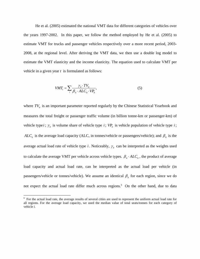
He et al. (2005) estimated the national VMT data for different categories of vehicles over

the years 1997-2002. In this paper, we follow the method employed by He et al. (2005) to

estimate VMT for trucks and passenger vehicles respectively over a more recent period, 2003-

2008, at the regional level. After deriving the VMT data, we then use a double log model to

estimate the VMT elasticity and the income elasticity. The equation used to calculate VMT per

vehicle in a given year t is formulated as follows:

, (5)it itt

i it it it

TVVMT

ALC VP

where itTV is an important parameter reported regularly by the Chinese Statistical Yearbook and

measures the total freight or passenger traffic volume (in billion tonne-km or passenger-km) of

vehicle type i ; it is volume share of vehicle type i ; itVP is vehicle population of vehicle type i ;

itALC is the average load capacity (ALC, in tonnes/vehicle or passengers/vehicle); and it is the

average actual load rate of vehicle type i . Noticeably, it can be interpreted as the weights used

to calculate the average VMT per vehicle across vehicle types. it itALC , the product of average

load capacity and actual load rate, can be interpreted as the actual load per vehicle (in

passengers/vehicle or tonnes/vehicle). We assume an identical it for each region, since we do

not expect the actual load rate differ much across regions.6 On the other hand, due to data

6 For the actual load rate, the average results of several cities are used to represent the uniform actual load rate for all regions. For the average load capacity, we used the median value of total seats/tonnes for each category of vehicle i.

28

limitations, we only obtain total freight or passenger traffic volume, itTV , for buses and trucks,

and therefore our estimations of VMT per vehicle are limited to these two types of vehicles.7

Figure 7 shows the average estimated VMT per vehicle and its standard deviation across

provinces for passenger vehicles and trucks from 2003-2009.

Figure 7. VMT per vehicle, 2003-2009

Note: Error bars indicate standard deviation.

7 Because the VMT we calculate is total VMT, not just VMT from gasoline-fueled cars. However, gasoline-fueled cars comprise the majority of cars in China: in 2007 they were approximately 75% of all vehicles, according to a Chinese government report (Development Center, 2007). While not perfect, our measure of VMT is highly correlated with the actual gasoline-fueled VMT, and it is the best we can do given the data limitations.

29

As seen in Figure 7, there is a decreasing trend of VMT per vehicle for passenger

vehicles (buses), while VMT per vehicle for trucks is increasing except for 2009. The

decreasing trend of VMT for buses conforms to He et al. (2005)’s estimation over the period

1997-2002, which is mainly due to the intensively increasing population share of small buses.

Although there is a rising share of light trucks, the share of heavy trucks is also climbing.

Therefore, the combined effects result in an increasing trend of VMT per vehicle for trucks over

the period 2003-2008 but a downward trend from 2008 to 2009.

3.2 VMT elasticities

To estimate the VMT price elasticity, we utilize a double log similar to the one we used to

calculate the gasoline elasticity:

0 1 2ln ln ln . (6)it it it itVMT P Y

To be consistent with our estimation of gasoline elasticity, we used VMT per capita as dependent

variable in the above model. VMT per capita is derived by multiplying VMT per vehicle by total

vehicle population and then dividing by total population. The regression results are shown in

Table 10. The intermediate-run VMT elasticity is estimated to be between -0.882 and -0.579.8

8 Crude oil price as instrument is not shown because there is no regional variation of crude oil price across province, thus resulting in the model to be unidentified due to a singularity problem. We incorporated fixed effects in the model because the Hausman test preferred fixed effects over OLS with a significant improvement in the R-squared, whereas for the gasoline demand model the Hausman test preferred OLS and the R-squared was not much improved by fixed effects.

30

Table 10. Double log model for VMT elasticity estimation

Dependent variable is log per capita VMT

OLS (without instruments) Diesel Price as IV

log real gasoline price -0.579** -0.882*** (0.193) (0.214)

log real income -0.066 -0.123 (0.08) (0.083)

Constant 4.813* 8.107*** (2.348) (2.572)

Observations 158 144 R-squared 0.507 0.4579 Notes: Standard errors in parentheses. Significance codes: * significant at 5%; ** significant at 1% *** significant at 0.1%. 3.3 Discussion of VMT elasticities

To compare our results with previous studies, a review of the previous literature on VMT

elasticities is shown in Table 11.

Table 11. Review of previous studies of VMT elasticities

VMT price elasticity VMT income elasticity

Country Estimation period

Short run

Intermediate run

Long run

Short run

Intermediate run

Long run

Dependent Variable

Source

US Pre-1986 -0.16 -0.32 Vehicle-km Goodwin (1992)

US Pre-1986 -0.15 -0.30

Vehicle-km Graham and Glaister (2002)

US Pre-1974 -0.54 0.30 Vehicle-km Goodwin et al. (2004) US 1974-1981 -0.32 0.57 0.21 Vehicle-km Goodwin et al. (2004) US Post-1981 -0.10 -0.24 -0.29 0.30 0.49 0.73 Vehicle-km Goodwin et al. (2004)

US Pre-1991 -0.10 -0.51 -0.30 -0.005 0.06 0.17 Per vehicle Goodwin et al. (2004)

China 2003-2009 -0.88 to -0.58 insignificant Per capita This study

Our estimates of the VMT price elasticity are somewhat higher in magnitude than the

estimates for other countries, but still in a reasonable range. The estimates from previous

estimates are for developed countries. A possible reason is that our estimates for China are

somewhat more elastic is that drivers in China might be more responsive to gasoline price

changes, thus leading to an elastic VMT, whereas the gasoline consumption is relatively inelastic

because the gasoline demand from industries other than transportation are relatively rigid while

the gasoline consumption share of transportation sector, which may exhibit a relatively greater

elasticity of demand for gasoline, has been shrinking over the years.

Our estimates of the VMT per capita income elasticity are statistically insignificant. As

shown in the Table 11, most estimates of the income elasticity of total VMT have a positive

value, while a few studies of VMT per vehicle indicate that a small negative income elasticity

might be reasonable because of the increasing density of cities and improved public

transportation system (CAERC, 2012). Thus, while total VMT may increase when incomes

increase, the VMT per capita may not necessarily increase.

There are concerns regarding our estimation of the VMT elasticity, mostly due to the

poor data quality of VMT data. The R2’s from our regressions are low, ranging from 0.46 to

0.51, suggesting that our model does not fully capture the determinants of VMT. As mentioned

above, due to lack of official reports of VMT and limited previous studies, our approximation of

VMT from the regularly reported traffic volume is not precise. However, we believe that our

estimates at least capture some of the variation in VMT across regions and years, that they are

still in a reasonable range consistent with previous estimates of VMT elasticities in the United

States and that they shed some light on consumers’ demand for VMT.

33

4 Discussion and conclusion

In this paper we use the basic double log model and several alternative specifications to

estimate the price and income elasticities of gasoline demand in China over the period 1997-

2008. Our models produce significant estimates of the price elasticity ranging between -0.497

and -0.196 and significant estimates of income elasticity ranging between 1.01 and 1.05. After

comparative analysis with earlier studies for developing countries, we believe our estimation

results are consistent and robust. The low price elasticity of gasoline demand indicates that

consumers are not sensitive to higher prices. One hypothesis is that with the rapid increase of

income and thus a lower budget share of gasoline consumption, consumers’ responses to higher

prices have decreased in magnitude, a hypothesis which is supported by a significant and

positive coefficient on the price-income interaction term. In addition, the relatively higher

income elasticity implies that increases in disposable income have caused gasoline consumption

to soar, largely due to the increasing ownership of cars.

Using the double log model and instrumental variables, we estimate the intermediate-run

VMT elasticity to be between -0.882 and -0.579. Although there are some concerns regarding the

validity of our estimated VMT data, our estimation results at least shed some light. Given a

higher intermediate-run VMT price elasticity than gasoline price elasticity and given improved

fuel efficiency, it might be the case the demand for gasoline is relatively more elastic in the

transportation sector than it is in other sectors. 9 If this is the case, imposing a gasoline

consumption tax to increase gasoline prices might be more effective in reducing gasoline

consumption, congestion and roadway pollution within the transportation system than it would

9 We do not have sufficient data to verify this, but obtaining the data in order to do so will be the subject of future work.

34

be in reducing the gasoline consumption in other sectors, although the current tax may be too

low to completely counteract the income effects.

A few policy implications can be drawn from our elasticity results. Currently China is

implementing a modest gasoline consumption tax, at 1 Yuan per liter. However, given that the

price elasticity is lower in magnitude than the income elasticity, a further increase in the gasoline

consumption tax will be needed to achieve the goal of gasoline consumption reduction. Ceteris

paribus, given the current income increase rate of 6%-8%, an increase of gasoline price by 18%-

23% is needed to counteract income effects for one year, not to mention achieve the goal of

gasoline consumption reduction. Table 12 presents the projected gasoline consumption growth

rate and associated greenhouse gas emissions growth rate the year following the implementation

of a tax under three gasoline tax specifications: 0%, 15% and 30%. As shown from the table, a

gasoline tax rate of 15%, which is close to the current volume based tax rate of 1 Yuan/liter, is

not sufficient to achieve the goal of gasoline consumption reduction in the following year. While

a more aggressive tax rate of 30% manages to meet the goal, it is likely to be politically

infeasible. As it is always politically difficult to implement a high gasoline consumption tax,

alternative measures such as public transportation, increases in fuel efficiency and mandates to

control potential vehicle population will be needed in the future.

35

Table 12. Projected gasoline consumption growth rate

Projected gasoline consumption (and associated CO2 emissions) growth rate

Gasoline Price Elasticity

Tax Rate Mid-range (-0.35) Low (-0.497) High (-0.196)

0% 6.18% 6.18% 6.18%

15% 0.93% -1.28% 3.24%

30% -4.32% -8.73% 0.30%

Notes: We assume the growth rate of real income per capita is 6% and income elasticity of gasoline consumption is 1.03, which is the midpoint of our estimation range. It is also assumed all increases in the gasoline price come from the tax increase.

36

References

Cao, J., and Zeng, J., 2010. The incidence of carbon tax in China. Working paper presented at

Lincoln Institute China Program Annual May Conference, Cambridge, USA, May 17,

2010

Cheng, K., Thomson, E., 2004. The demand for gasoline in China: A cointegration analysis.

Journal of Applied Statistics, 31(5), 533-544.

China Automotive Energy Research Center, 2012. China Automotive Energy Outlook 2012.

Science Press, 978-7-03-0327963-3.

Dahl, C. A., 1979. Consumer adjustment to a gasoline tax. The Review of Economics and

Statistics, 6(3), 427-432.

Development Center of State Council for Industry Research, 2007. Diesel technology and

development policy.

Edlin, A. S., Mandic, P. K., 2006. The Accident Externality from Driving. Journal of Political

Economy,114.5, 931-955.

Eltony, M. N. & Al-Mutairi, N. H., 1995. Demand for gasoline in Kuwait: an empirical analysis

using cointegration techniques. Energy Economics, 17(3), 249–253.

Environmental Protection Agency [EPA], 2009. Climate Change. Cited 31 March 2009.

URL:http://www.epa.gov/climatechange/basicinfo.html

37

Fullerton, D., West, S., 2003. Public Finance Solutions to Vehicle Emissions Problems in

Californa. The Berkeley Electronic Press. http://www.bepress.com/fullertonwest

Goldberger, A.S., 1991. A course in econometrics. Harvard University Press, Cambridge, MA.

Goodwin, P. B., 1992. A review of new demand elasticities with special reference to short and

long run effects of price changes. Journal of Transport Economics and Policy, 26, 155–

163.

Goodwin, P. B., Dargay, J. & Hanly, M., 2004. Elasticities of road traffic and fuel consumption

with respect to price and income: a review. Transport Reviews, 24(3), 275-292

Graham, D. and Glaister, S., 2002. The demand for automobile fuel: a survey of elasticities,

Journal of Transport Economics and Policy, 36(1), 1–26.

Graham, D. J. and Glaister, S., 2004. Road traffic demand elasticity estimates: a review,

Transport Reviews, 24(3), 261–274.

Guojiatongjiju, (State Statistical Bureau, Department of Industrial and Transportation Statistics)

Zhong guo neng yuan tong jinian jian 2000-2010 (China Energy Statistical Yearbook

1997-2010)

He, K., Huo, H., Zhang, Q., He, D., An, F., Wang, M., Walsh, M., 2005. Oil consumption and

CO2 emissions in China’s road transport: current status, future trends, and policy

implications. Energy Policy, 33 (2005) 1499–1507

38

Houthakker, H. S., Verleger, P. K. and Sheehan, D. P., 1974. Dynamic Demand Analysis for

Gasoline and Residential Electricity. American Journal of Agricultural Economics, 56(2)

412-418.

Hughes, J., Knittel, C., Sperling, D., 2008. Evidence of a Shift in the Short-Run Price Elasticity

of Gasoline Demand. The Energy Journal, 291, 93-114.

Liao, H. & Lee, Y., 2007. Chinese gasoline and diesel demand. Working paper.URL:

http://www.usaee.org/usaee2009/submissions/OnlineProceedings/Liaopaper32IAEE.pdf

Li, H. & Zax, J.-S.J., 2003. Labor supply in urban China. Journal of Comparative Economics,

31 (4) (2003) 795–817.

Lin, C.-Y.C., 2011. Estimating supply and demand in the world oil market. Journal of Energy

and Development, 34 (1), 1-32.

Lin, C.-Y.C. & Prince, L., 2009. The optimal gas tax for California.Energy Policy, 37 (12),

5173-5183.

Lin, X., Tang, D., Ding, Y., Yin, H., Ji, J., 2009. Study on the Distribution of Vehicle Mileage

Travelled in China. Research of Environmental Sciences, 22(3).

Lingdian Consulting firm, 2009. Futian Index. URL:

http://auto.sina.com.cn/csgc/q0904/index.shtml

McRae, R., 1994. Gasoline demand in developing Asian countries. Energy J 15(1), 143-155.

39

Mankiw, G., 2006. The Pigou Club Manifesto. http://Gregmankiw.blogspot.com/2006/10/pigou-

club-manifesto.htm.

Parry, I., Small, K., 2004. Does Britain or the United States Have the Right Gasoline Tax?

Resources for the Future Discussion Paper, 02-12 rev.

Parry, I., Small, K., 2005. Does Britain or the United States have the right gasoline tax?

American Economic Review, 95, 1276-1289.

Ramanathan, R., 1999. Short- and long-run elasticities of gasoline demand in India: an empirical

analysis using cointegration techniques. Energy Economics, 21(4), 321–330.

Ramsey, Frank P., 1927. A Contribution to the Theory of Taxation.Economic Journal,37, 47-61.

Ramsey, J., Rasche, R. and Allen, B., 1975. An Analysis of the Private and Commercial Demand

for Gasoline. The Review of Economics and Statistics, 57(4),502-507.

Wang, Y., Teter, J., Sperling, D., 2011. China's soaring vehicle population: Even greater than

forecasted? Energy Policy, 39(6), 3296-3306

Watts, J., 2009. China’s E6 electric car: “we’re not trying to save the world- we’re trying to

make money”. URL: http://www.businessgreen.com/bg/news/1801462/chinas-e6-

electric-car-were-trying-save-world-trying-money