Master’s thesis · 30 hec · Advanced level European Erasmus Mundus Master Program: Agricultural Food and Environmental Policy Analysis (AFEPA) Degree thesis No 1047 · ISSN 1401-4084 Uppsala 2016

iiii

Elasticity of demand for gasoline in Sweden

Emma Dahlkvist

iiii

Elasticisty of demand for gasoline in Sweden

Emma Dahlkvist

Supervisor: Rob Hart, Swedish University of Agricultural Sciences, Department of Economics

Assistant supervisor: Thomas Heckelei, Rheinische Friedrich-Wilhelms-Universität

Examiner:

Bonn, Institute for Food and Resource Economics

Sebastian Hess, Swedish University of Agricultural Sciences, Department of Economics

Credits: 30 hec Level: A2E Course title: Independent project/degree in Economics Course code: EX0537 Programme/Education: European Erasmus Mundus Master Program: Agricultural Food and Environmental Policy Analysis (AFEPA) Faculty: Faculty of Natural Resources and Agricultural Sciences

Place of publication: Uppsala Year of publication: 2016 Name of Series: Degree project/SLU, Department of Economics No: 1047 ISSN 1401-4084 Online publication: http://stud.epsilon.slu.se

Keywords: Distributional effects, Fuel tax, Gasoline price elasticity, Income elasticity

iii

Declaration

I hereby affirm that I have prepared the present paper self-dependently, and without the use of any other tools than the ones indicated. All parts of the text, which were taken over verbatim or analogously from published or unpublished works have been identified accordingly. The thesis has not yet been submitted in the same or a similar form, within the context of another examination.

_______________________ _______________________ Date, place of submission Emma Dahlkvist

iv

Abstract Policy measures in the transport sector have been widely debated during the recent decades, specifically in terms of increasing carbon emissions from passenger transport. Fuel taxes is receiving most receptive consideration by governments, although households tend to respond little to these measures, especially in rural regions. The aim of this paper, which focuses at the gasoline consumption among households, is to develop a model to estimate price and income elasticities in rural and urban regions in Sweden. While obtaining overall price elasticity to be within the range of previous studies, I find that there is a significant variation in price elasticities across regions. As a consequence, these differences might result in unwanted distributive effects.

v

CONTENTS

DECLARATION III ABSTRACT IV 1. Introduction 1

2. The transport sector 3 2.1. Fuel consumption and gasoline price in Sweden 4 2.2. Transport policy 4 2.3. Fuel tax 5 2.4. Motivations of increasing the fuel tax in Sweden 6 2.5. The distributional effects of environmental taxes 7

3. Theoretical framework 8 3.1. Neoclassical consumer demand theory 8 3.2. Substitutes and complement goods 10 3.3. Consumer production theory 10 3.4. Elasticity 10

4. Data and method selection 11 4.1. Data 11

5. Methodology 12 5.1. My model 12 5.2. Potential drawbacks with single equation model 16 5.3. Demand systems 17

6. Model specification 18 6.1. Interaction Parameter Model 18 6.2. Heckman selection specification 19

7. Results and discussion 20

8. Conclusion 25 8.1. Ethical considerations 26 8.2. Future studies 26 References 27 Appendix A.

Variable definition 31

vi

1. Introduction

In January of 2016 the Swedish government initiated an increase of thefuel tax with the aim to reduce carbon emissions and energy dependencein the transport sector. Whether this aim is reachable will depend on howhouseholds response to this increased tax. This response can be measuredwith elasticities, which indicate how much more or less a household de-mand as the price of the gasoline change. Gasoline elasticities have beenfound to vary within countries depending on household income as well aslocation. These differences might cause unwanted distributive effects wheresome households are more punished that others.

In urban areas it is reasonable to suppose that the long run price elasticityof demand for fuel is rather high, since there are many alternatives to cartransport. On the other hand, in rural areas with fewer options for publictransport and where work and home may be far apart, the fuel demand maybe less price sensitive. In the worst case, the high fuel tax may be seen asa punitive charge applied to those living in the countryside, who are unableto adapt their behaviour to avoid its effects.

For reasons both of equity and policy effectiveness, it is relevant to recog-nise how an increase in fuel tax will affect different types of households.It is also useful to know from which groups the demand response will bemost distinct. In this setting, whether rural households in Sweden are likelyto be more affected and more responsive to fuel taxes compared to urbanhouseholds, is contingent on an analysis of price and income elasticities ofgasoline demand.

The research question of this study is whether households have differentprice and income elasticities of gasoline demand in Sweden, depending onin which region they are located. The aim is thus to test the potential exis-tence of a difference in the elasticity of demand of gasoline fuel by Swedishhouseholds, given their place of residence. To do so an econometric modelis assessed with annual disaggregate data from the Swedish Household Ex-penditure Survey of the period between 2003-2009 and 2012. The price andincome elasticities of the demand of gasoline is compared for householdslocated in the major towns in Sweden with households living in rural andother regions. Conclusions are drawn on the effectiveness and distributionalimpacts of the tax increase.

Many studies have used disaggregate data to find the regional effect of aprice shock in car fuel. This have been done by including location of thehousehold as a variable in the model (e.g., Poterba, 1991; Kayser, 2000;Bento et al., 2009; West and Williams, 2004). Fewer studies intend to morespecifically measure the actual price elasticity of each region and its impli-cations.

Bureau (2011) studies the distributive effects of an increased fuel tax inFrance with panel data from 2003-2006, and distinguishes between urbanand peri-urban/rural households that own a car. The estimated elasticitiesin the former region are between -0.30 for low income households to -0.19for high income households and for the peri-urban/rural -0.25 to -0.17. Inthe UK Blow and Crawford (1997) and Santos and Catchesides (2005) usethe same data source in different time periods. Blow and Crawford (1997)

1

examine an earlier time period of 1988-1993 and find the greatest priceelasticity to be -0.54 of poor households in urban areas and the smallestto be rich households in rural areas of -0.2. The income elasticity showslittle variation with respect to population density and is on average 0.26.Santos and Catchesides (2005) study the time period 1999-2000, and find thegreatest price sensitivity to be among the poor households living in urbanareas of -0.93. The smallest price response is for households living in ruralareas, where middle-income households has the smallest price response withan elasticity of -0.75. Income elasticity is found to be 0.63 for households inthe urban areas and 0.6 for households in the rural areas.

These studies show that households in the more densely populated re-gions, in general, tend to be more price sensitive to gasoline than householdsin the rural areas, and that urban households might have greater income re-sponse than the rural ones.

In Sweden however the pattern seems to be different, based on the verylimited number of studies. Brannlund and Nordstrom (2004) study theperiod 1985, 1988 and 1992 and predict price elasticities to be consistentaround -0.99, regardless of the location of the household. Although Brannlundand Nordstrom use a more sophisticated modelling approach in relation tothe studies listed above, these results are quite contradictory even to studiesusing the same modelling approach. Nicol (2003) applies a similar method-ology as Brannlund and Nordstrom (2004) and find Canadian householdsto vary in price elasticity estimates between -0.47 to -0.83 depending ontheir location. Nicol indicate that while elasticities might change due tocertain characteristics of a household, this might not be the same in anothercountry. Thus, there is a need for them to be country specific.

The small number of elasticity studies of gasoline in the different regionsin Sweden is the main motivation of this study. While previous studies ofincreased fuel taxes tend to focus on the income equity issue, this study willmainly focus on the effect on the different regions. In the methodology part,an alternative approach applicable in a single demand function is used toestimate elasticities, by including interaction terms between several regionsand gasoline price as well as income. Interaction terms of this kind havepreviously been used by Wadud et al. (2010), although not in the Swedishcase.

In this thesis gasoline demand is modelled as a function of price, totalexpenditure and other relevant household characteristics. The goal of themodel is to assess the influence of prices on fuel consumption and the dis-tributive effects on households in different regions. The model is calibratedon five different regions in Sweden, with rural and non-rural characteris-tics. Price and income elasticity are estimated, by using the static singleequation model. In order to derive the elasticity estimates directly from theestimated coefficients the static log-log linear model is used with the ordi-nary least square regression (OLS) in line with previous gasoline demandstudies (e.g Hughes et al., 2008). In Hughes’s model specification of the log-log linear OLS, no household characteristics are included. In my model onthe other hand various aspects of the model is considered based on the dataat hand and findings in the literature, specifically; time, regional-dimension,

2

demographic characteristics. The time trend is included as fixed time effectsusing dummy variables representing each year. In addition also the regionaleffect will be studied using dummy variables. Further since the interest is tosee how elasticities varies with the regions interaction terms region-price andregion-expenditure is integrated, following Wadud et al. (2010) approach aswell as other household demand studies (e.g. Archibald and Gillingham,1980).

Households characteristics included in the model are based on empiricalfindings in the literature. Kayser (2000) suggests that demographic charac-teristics such as income, age and occupation status affect gasoline demand,while education level have no significant impact on demand.

With considerations to the data, where about 20 percent of householdsreport zero consumption for gasoline, the OLS regression is not appropri-ate to use for the whole sample since it does not take special account ofzero gasoline expenditure and consequently yield inconsistent estimates ofthe parameters. Therefore, subsample OLS including only households withpositive expenditure on gasoline will be tested. Wales and Woodland (1983)indicate however that this will reduce the sample size and the standardestimators may be biased and inconsistent. In order to correct for thesepotential sample selections issues Heckman’s two stage approach is used.

The results indicate a significant variation of the price elasticities in thedifferent regions in Sweden. Urban households tend to be more responsive togasoline prices, particularly in Stockholm, Gothenburg and Malmo. Whilerural households in the northern regions seem to be almost price insensitive.With regards to the income elasticity, the regional location of the householddoes not seem to affect the level. These are measures in the intermediaterun and effects in the long run will partly depend on how the revenue of thetax increase is recycled.

Past decades of urbanization and depopulation of rural areas in Swedenhas lead to extensive engagement into rural development strategies by theSwedish government. Substantial investments are directed towards this pol-icy area in order to maintain the livelihood of remote regions. Within thiscontext, transport is a main component. Thus if strict transport policieshurt households living in rural areas, these measures might contradict withinvestments supporting these regions. The region specific elasticity estimatesof gasoline demand resulting from this study might therefore be desirablefor policy-makers in order to design overall policy measures more efficiently.

Next section will review and discuss the transport sector in Sweden. Fol-lowing the theoretical framework of this study is presented with focus onthe neoclassical framework. Section 4 discuss the data applied in this thesis,followed by a review of my model and alternative approaches that couldhave been chosen. Section 6 specifies the final model, followed by the resultsand discussion. Lastly section 8 concludes the paper.

2. The transport sector

In this section, the general transport policy in Sweden is discussed andmore specifically the recent increase in the fuel tax and the distributiveeffects it might result in.

3

Our modern society is highly dependent on a functioning transport sys-tem. While mobility is a crucial feature of our lifestyle and passenger trans-port is relevant for economic development together with individual and socialwelfare, it also causes a number of serious environmental and health prob-lems. The level and increasing trend of automobile fuel consumption as wellas the dependence of fossil fuel as energy source is a growing concern amongcountries, particularly in terms of increasing carbon emissions and securityof energy supply. Although policy measures that discourage fossil fuel usein transport are in place and alternative fuels are available, passenger trans-port is still the fastest growing emitter of carbon emissions worldwide of allenergy source sectors (IPCC, 2015).

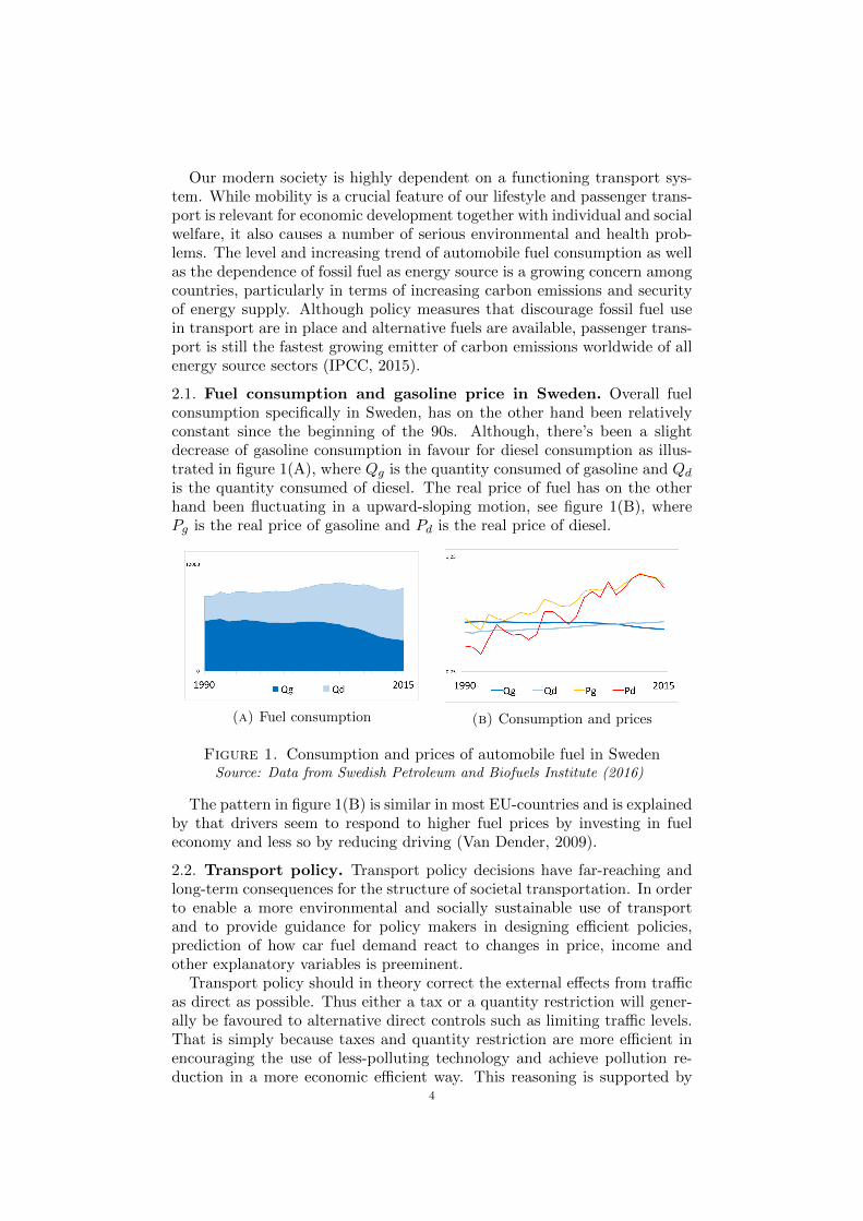
2.1. Fuel consumption and gasoline price in Sweden. Overall fuelconsumption specifically in Sweden, has on the other hand been relativelyconstant since the beginning of the 90s. Although, there’s been a slightdecrease of gasoline consumption in favour for diesel consumption as illus-trated in figure 1(A), where Qg is the quantity consumed of gasoline and Qdis the quantity consumed of diesel. The real price of fuel has on the otherhand been fluctuating in a upward-sloping motion, see figure 1(B), wherePg is the real price of gasoline and Pd is the real price of diesel.

(a) Fuel consumption (b) Consumption and prices

Figure 1. Consumption and prices of automobile fuel in SwedenSource: Data from Swedish Petroleum and Biofuels Institute (2016)

The pattern in figure 1(B) is similar in most EU-countries and is explainedby that drivers seem to respond to higher fuel prices by investing in fueleconomy and less so by reducing driving (Van Dender, 2009).

2.2. Transport policy. Transport policy decisions have far-reaching andlong-term consequences for the structure of societal transportation. In orderto enable a more environmental and socially sustainable use of transportand to provide guidance for policy makers in designing efficient policies,prediction of how car fuel demand react to changes in price, income andother explanatory variables is preeminent.

Transport policy should in theory correct the external effects from trafficas direct as possible. Thus either a tax or a quantity restriction will gener-ally be favoured to alternative direct controls such as limiting traffic levels.That is simply because taxes and quantity restriction are more efficient inencouraging the use of less-polluting technology and achieve pollution re-duction in a more economic efficient way. This reasoning is supported by

4

findings in the literature (e.g De Jong and Gunn, 2001) where price elasticityof gasoline is generally higher in absolute terms, than the price elasticity ofautomobile travel demand.

When governments initiate passenger transport policies, they are usuallydriven by four types of concern: the tax base, climate change, the securityof oil supply, profits and employment in the domestic car industry (Proostand Van Dender, 2011). Since Sweden is part of the European Union, theoutline of the transport policies are partly affected by regulations settled inthe Union. In 2009, the European Commission passed a legislation requiringcar producers to reduce the average per-kilometre carbon emissions of newlymanufactured automobiles to 130g/km by 2015 (Council of the EuropeanUnion, 2009). In addition to this fuel efficient standards, minimum rates offuel taxation are set for all member states (Council of the European Union,2003).

There are divided opinions in the literature regarding the effectivenessof combining fuel efficiency standards with fuel taxes. While Van Dender(2009) suggest that fuel efficiency standards and fuel taxes are complementsrather than substitutes, more recent studies by Frondel and Vance (2013)and Liu (2015) demonstrate that tightening efficiency standards will par-tially offset the effectiveness of taxes on reducing fuel consumption, sincethe improvements of vehicle fuel efficiency leads to lower price elasticityand weakens the consumer response to gasoline price changes. Although,according to Sperling and Nichols (2012) a collection of different policy in-struments are needed in order to have large emission reductions from thetransport sector.

Despite policy efforts within the EU, technical progress and potentialfor cost-effective energy efficiency improvements, the transport system hasnot fundamentally changed and is not sustainable (Akerman et al., 2000).Recent political activities suggests that transport charges and taxes mustbe reconstructed in the direction of application of the ”polluter-pays” and”user-pays” principle (European Commission et al., 2011).

2.3. Fuel tax. Among the policies used in the transport sector, fuel taxesseem to be receiving most receptive consideration by governments as theyraise revenue but also through their effect on price that can affect demandand consumption (Nicol, 2003). That is also true in Sweden, where thegovernment support the economists’ idea of fuel taxes being of central im-portance to meet the climate and energy objectives in a cost effective manner(The Swedish Government, 2015).

The use of the price mechanism is particularly important due to its con-tribution to revenue of the public fund, but also to assist markets to operatemore efficiently by ensuring that the the external cost of using a vehicle aremet by the users.

Figure 2 show the four components of the gasoline price met by householdsin Sweden: the gross margin, production cost, tax and Value Added Tax.

Taxation of automobile fuel in Sweden consist of excise duties (tax) andvalue added tax. Excise duties are divided into energy tax and carbon taxand are derived on the basis of the national Energy Tax Act(1994:1776).The carbon tax was introduced to reduce carbon emissions from fossil fuels,

5

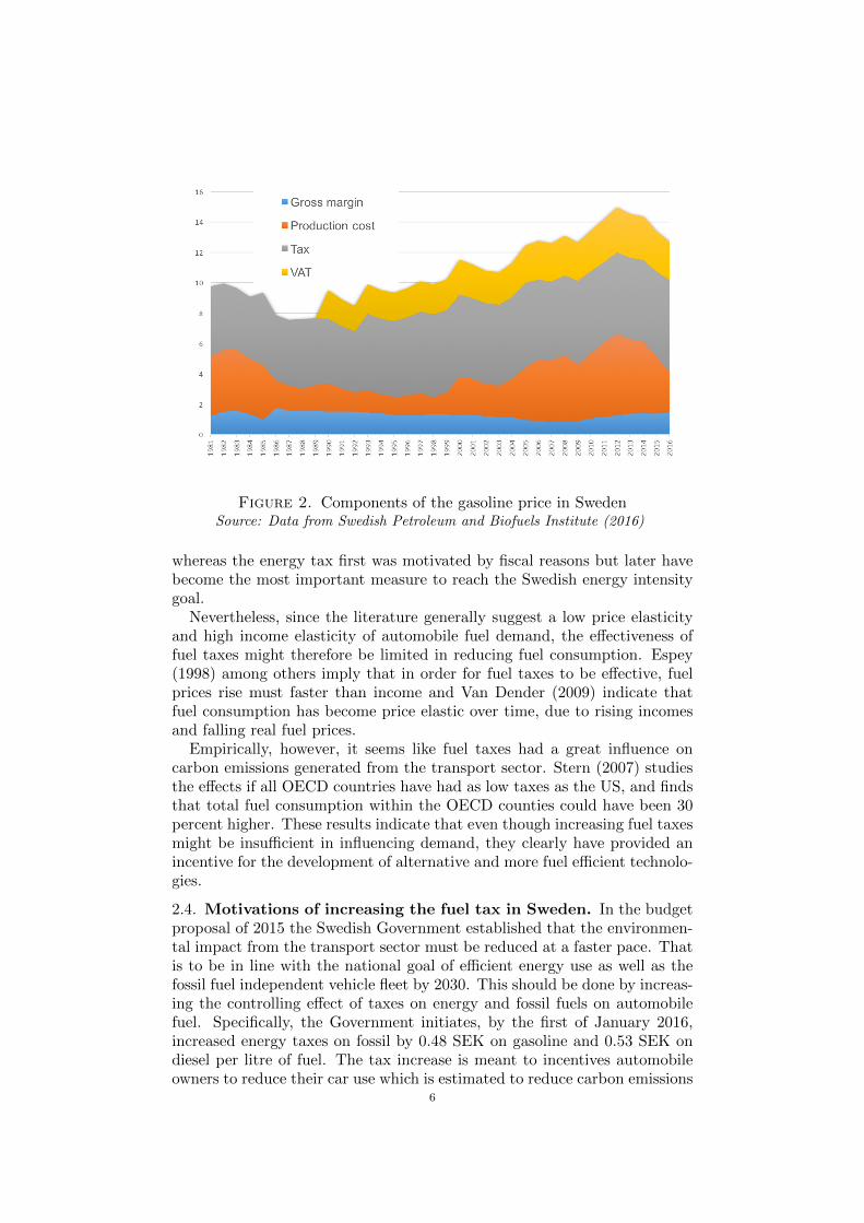
Figure 2. Components of the gasoline price in SwedenSource: Data from Swedish Petroleum and Biofuels Institute (2016)

whereas the energy tax first was motivated by fiscal reasons but later havebecome the most important measure to reach the Swedish energy intensitygoal.

Nevertheless, since the literature generally suggest a low price elasticityand high income elasticity of automobile fuel demand, the effectiveness offuel taxes might therefore be limited in reducing fuel consumption. Espey(1998) among others imply that in order for fuel taxes to be effective, fuelprices rise must faster than income and Van Dender (2009) indicate thatfuel consumption has become price elastic over time, due to rising incomesand falling real fuel prices.

Empirically, however, it seems like fuel taxes had a great influence oncarbon emissions generated from the transport sector. Stern (2007) studiesthe effects if all OECD countries have had as low taxes as the US, and findsthat total fuel consumption within the OECD counties could have been 30percent higher. These results indicate that even though increasing fuel taxesmight be insufficient in influencing demand, they clearly have provided anincentive for the development of alternative and more fuel efficient technolo-gies.

2.4. Motivations of increasing the fuel tax in Sweden. In the budgetproposal of 2015 the Swedish Government established that the environmen-tal impact from the transport sector must be reduced at a faster pace. Thatis to be in line with the national goal of efficient energy use as well as thefossil fuel independent vehicle fleet by 2030. This should be done by increas-ing the controlling effect of taxes on energy and fossil fuels on automobilefuel. Specifically, the Government initiates, by the first of January 2016,increased energy taxes on fossil by 0.48 SEK on gasoline and 0.53 SEK ondiesel per litre of fuel. The tax increase is meant to incentives automobileowners to reduce their car use which is estimated to reduce carbon emissions

6

slightly. In addition, the Government believe that higher energy taxes mayalso result in automobile owners to choose energy-efficient vehicles, whichcould lead to further carbon reductions. In order for this aim to be ful-filled it’s important to examine the consumer response to the price change.The theoretical framework for doing so will be explained further in the nextchapter.

2.5. The distributional effects of environmental taxes. With an in-creased taxation on fuel, households will be affected differently dependingon their income and their reliance to travel by car. The change in fuel taxeswill therefore generate distributional effects depending on household char-acteristics. There are many studies focusing on the income equity issue ofgasoline taxes. Bureau (2011), conclude that fuel tax is regressive in France,which also is true in the UK according to Santos and Catchesides (2005),who further concludes that middle-income households suffer the most.

Although, with an environmental tax, or a tax correcting for externaleffects, Eliasson et al. (2016) states that it might be unclear whether thesedistributional effects, when it comes to income equity, are relevant to con-sider. If the price of car travel is lower than the full social cost, those whodrive the most should also bear the burden of the cost of external effects.The economic welfare effect on households due to a tax increase, is theoret-ically the same for all regardless of income or wealth, if they face the sameprice. The strive for income equity among households is rather handled bytaxation and welfare systems.

However, when discussing distributional effects, there are other aspects toconsider such as the regional dimension of the household. Within this areathere a much fewer studies in the literature. Bureau (2011) finds that welfarelosses are significantly higher in rural areas when distinguishing betweenurban and rural residents in France. In Sweden Eliasson et al. (2016) findsthe same pattern.

The regional dimension of the distributional impacts of an increased fueltax may be of high interest in Sweden. That is since the government investsa substantial amount into rural development strategies due to decades of in-creased urbanisation causing depopulation of some rural areas. Within thispolicy area transport and infrastructure are two significant components.Thus if the transport policy cause negative distributional effects in ruralareas, these effects will counteract with the large investments in rural devel-opment.

Before getting into the theoretical framework for doing so, figure 3 illus-trates how the budget share put on automobile fuel differ between regions.Region 0 and 1 are the most populated in Sweden and region 3-4 the mostrural. This clearly illustrate that households in rural areas allocate a largeramount of their total expenditure towards gasoline consumption than otherhouseholds.

A complete analysis of the net welfare effect needs to consider the useof revenues from the tax are recycled. This could be read further in anextensive study by Bento et al. (2009) within the US context and Eliassonet al. (2016) who examine the Swedish prospective.

7

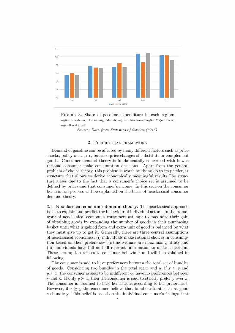
Figure 3. Share of gasoline expenditure in each region:reg0= Stockholm, Gothenburg, Malmo, reg1=Urban areas, reg3= Major towns,

reg4=Rural areas

Source: Data from Statistics of Sweden (2016)

3. Theoretical framework

Demand of gasoline can be affected by many different factors such as priceshocks, policy measures, but also price changes of substitute or complementgoods. Consumer demand theory is fundamentally concerned with how arational consumer make consumption decisions. Apart from the generalproblem of choice theory, this problem is worth studying do to its particularstructure that allows to derive economically meaningful results.The struc-ture arises due to the fact that a consumer’s choice set is assumed to bedefined by prices and that consumer’s income. In this section the consumerbehavioural process will be explained on the basis of neoclassical consumerdemand theory.

3.1. Neoclassical consumer demand theory. The neoclassical approachis set to explain and predict the behaviour of individual actors. In the frame-work of neoclassical economics consumers attempt to maximize their gainof obtaining goods by expanding the number of goods in their purchasingbasket until what is gained from and extra unit of good is balanced by whatthey must give up to get it. Generally, there are three central assumptionsof neoclassical economics; (i) individuals make rational choices in consump-tion based on their preferences, (ii) individuals are maximizing utility and(iii) individuals have full and all relevant information to make a decision.These assumption relates to consumer behaviour and will be explained infollowing.

The consumer is said to have preferences between the total set of bundlesof goods. Considering two bundles in the total set x and y, if x � y andy � x, the consumer is said to be indifferent or have no preferences betweeny and x. If only y � x, then the consumer is said to strictly prefer y over x.The consumer is assumed to base her actions according to her preferences.However, if x � y the consumer believe that bundle x is at least as goodas bundle y. This belief is based on the individual consumer’s feelings that

8

determine her choice. The belief and action processes are independent ofeach other, although put together they form the behaviour of the consumer(Deaton and Muellbauer, 1980).Mas-Colell et al. (1995) defines it (emphasis added),

The theory [of consumer behaviour] is developed by first im-posing rationality axioms on the decision maker’s preferencesand then analysing the consequences of these preferences forher choice behaviour (i.e. on decisions made)

The rationality axioms Mas-Colell et al. (1995) is referring to must be metby the consumer preference relations in order for her to be assumed to actrational. First the preferences must be complete, indicating that for anytwo consumption bundles x and y, x � y, y � x, or both. The second istransitivity which imply that for any three bundles x, y and q, if x � y andy � q, then x � q. The preferences must also be reflexive, where any bundleis at least as good as itself, and continuous, indicating no big jumps inconsumer preferences. Further that preferences are monotonicity, meaningthat more is always preferred to less and lastly that they are convex, whereany combination of two equally preferable bundles are more desirable thanthese bundles by themselves.

Given the completion of these axioms, the consumers indifference setsbetween bundles can be illustrated with indifference curves, in which eachcurve is the set of all bundles generating the same utility for the consumer.The slope of the line tangent to a bundle on the indifference curve is calledthe marginal rate of substitution, MRS, which implies the rate at whichthe consumer is willing to exchange x for y . This exchange also depends onthe prices of the goods as well as the constrained budget of the consumer.The most preferred bundle of goods the consumer can afford is found bychoosing the bundle on the budget line where MRS equals the price ratio.

In order for the consumer to be utility maximizing, stated by assumption(ii), the consumer will choose the bundle of goods that maximizes her utilitythe most constrained by her income. Consider an individual with an utilityfunction u(q, z) where q is the vector of a number of goods on which theconsumer must make consumption decisions and z represent the individual’scharacteristics. The total amount of income to spend is y, and the budgetconstraint is y = p′x where p′ is a vector of prices of the goods. Themaximizing utility problem facing the consumer is,

max u(q, z)

s.t y = p′x

The solution to the maximization problem is a set of demand equations forthe goods i in vector q,

qi = f(p, y, z)

From this demand equation we find that besides consumer choice strategies,consumption patterns are also affected by price changes. A consumer witha fixed budget in the short term has three possible responses due to a pricechange: (i) The consumer buy another good as a substitute; (ii) the con-sumer purchase less of the good and no substitute goods; (iii) the consumer

9

continue to buy the same amount of the good and decrease the expenditureon other goods in her consumption basket.

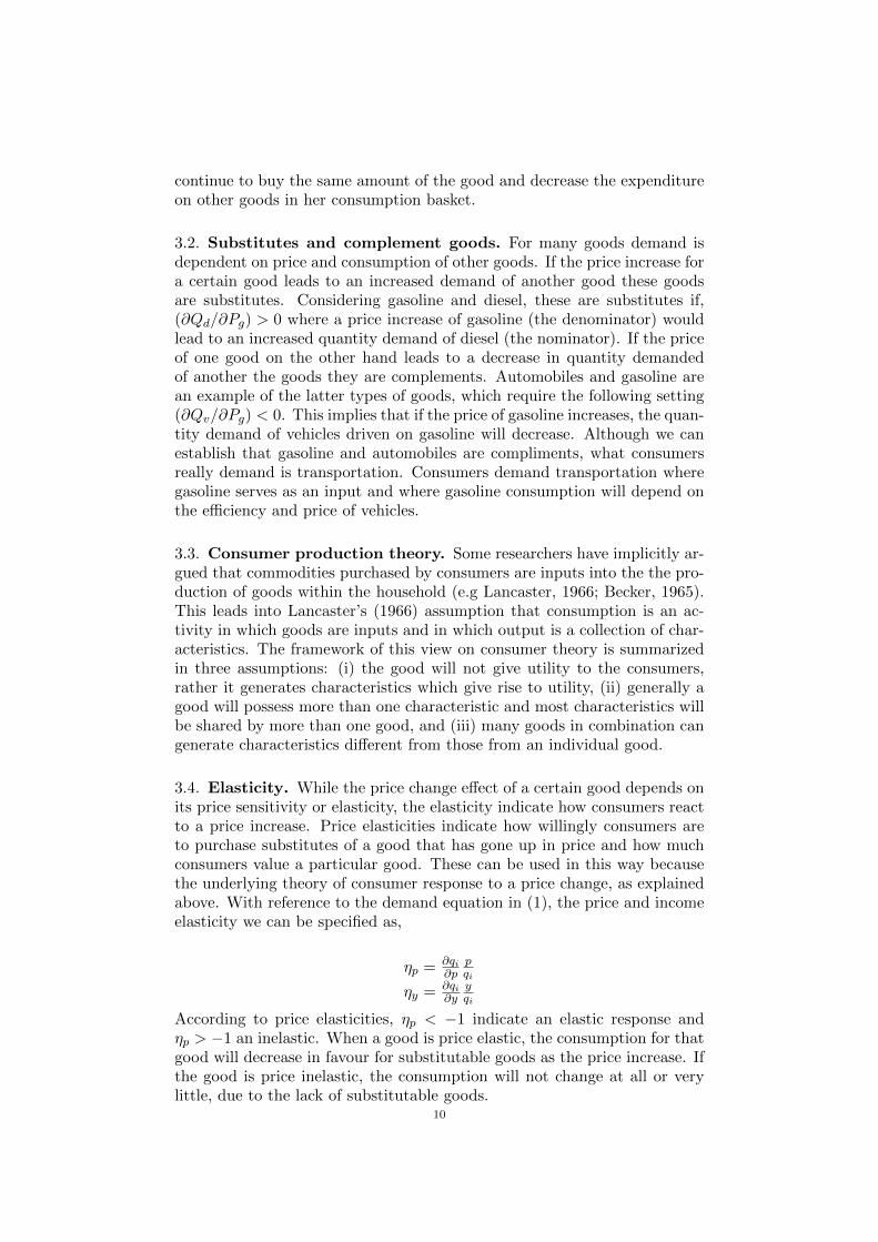
3.2. Substitutes and complement goods. For many goods demand isdependent on price and consumption of other goods. If the price increase fora certain good leads to an increased demand of another good these goodsare substitutes. Considering gasoline and diesel, these are substitutes if,(∂Qd/∂Pg) > 0 where a price increase of gasoline (the denominator) wouldlead to an increased quantity demand of diesel (the nominator). If the priceof one good on the other hand leads to a decrease in quantity demandedof another the goods they are complements. Automobiles and gasoline arean example of the latter types of goods, which require the following setting(∂Qv/∂Pg) < 0. This implies that if the price of gasoline increases, the quan-tity demand of vehicles driven on gasoline will decrease. Although we canestablish that gasoline and automobiles are compliments, what consumersreally demand is transportation. Consumers demand transportation wheregasoline serves as an input and where gasoline consumption will depend onthe efficiency and price of vehicles.

3.3. Consumer production theory. Some researchers have implicitly ar-gued that commodities purchased by consumers are inputs into the the pro-duction of goods within the household (e.g Lancaster, 1966; Becker, 1965).This leads into Lancaster’s (1966) assumption that consumption is an ac-tivity in which goods are inputs and in which output is a collection of char-acteristics. The framework of this view on consumer theory is summarizedin three assumptions: (i) the good will not give utility to the consumers,rather it generates characteristics which give rise to utility, (ii) generally agood will possess more than one characteristic and most characteristics willbe shared by more than one good, and (iii) many goods in combination cangenerate characteristics different from those from an individual good.

3.4. Elasticity. While the price change effect of a certain good depends onits price sensitivity or elasticity, the elasticity indicate how consumers reactto a price increase. Price elasticities indicate how willingly consumers areto purchase substitutes of a good that has gone up in price and how muchconsumers value a particular good. These can be used in this way becausethe underlying theory of consumer response to a price change, as explainedabove. With reference to the demand equation in (1), the price and incomeelasticity we can be specified as,

ηp = ∂qi∂p

pqi

ηy = ∂qi∂y

yqi

According to price elasticities, ηp < −1 indicate an elastic response andηp > −1 an inelastic. When a good is price elastic, the consumption for thatgood will decrease in favour for substitutable goods as the price increase. Ifthe good is price inelastic, the consumption will not change at all or verylittle, due to the lack of substitutable goods.

10

With respect to the income elasticity, a normal good can be classified interms of its importance to the consumer where, 0 < ηy < 1 are necessitygoods and ηy > 1 luxury.

The degree of elasticity depends on a number of factors, primarily theavailability of alternative (substitute) goods but also the consumer’s indi-vidual tastes and other infrastructural factors particularly in the contextof fuel. Given a consumer owns a gasoline car, gasoline will have limiteddegree of substitutability especially in the short term. Over time, however,the consumer has the option to purchase a vehicle that is more fuel efficientand/or use alternative fuels and still enjoy the same level of utility usingless fuel (if the infrastructure allows). Typically, switching vehicle requiresreplacing an expensive good and for many consumers it is considered a long-run adjustment to high fuel prices. Therefore, empirical estimates on priceelasticity of gasoline tend to be elastic in the long term and inelastic in theshort. There are several methods to estimate the elasticity of fuel demandthat will be further explained in section 5.

4. Data and method selection

In this section the underlying data of this study is discussed.

4.1. Data. The annual gasoline price used are the yearly average for petrolprovided by the Swedish Petroleum and Biofules Institute. In order to esti-mate consistent elasticities and to ensure identification of actual demand re-sponses, the prices are adjusted for inflation. To do so the annual ConsumerPrice Index (CPI) series, published by Statistics of Sweden on a monthlybasis, is used. The reference is the annual average of 2015.

The household data is collected from Statistics of Sweden between 2003-2009 and 2012. The data is based on the Swedish Household budget survey(HBS), including mainly household expenditure on consumption goods butalso household and individual characteristics. The data is repeated crosssectional with different households reporting each year but answering thesame type of questions. Due to the repeated cross sectional structure, theyearly samples are assumed to be independent. In order to efficiently com-bine the two sets of household characteristics and individual characteristics,the individual characteristics are based on the head of the household only.The total expenditure level will be used as a proxy for lifetime income, whichprevious studies suggest to be a better predictor of consumption than an-nual income (see Friedman, 1957; Poterba, 1991; West and Williams, 2004).The annual quantity of gasoline consumption will be derived by dividingthe annual household expenditure share spent on gasoline with the annualaverage price of gasoline.

In order to account for household features that may affect consumer be-haviour with respect to gasoline demand, we need to include these householdcharacteristics in the model estimation. A summary statistics for the vari-ables extracted from the HBS survey and included in my model to representhousehold characteristics are presented in 1. All of them have been shownto affect gasoline consumption (e.g Puller and Greening, 1999; West andWilliams, 2004; Kayser, 2000).

11

Table 1. Summary statistics

Statistic N Mean St. Dev. Min Max

Total annual expenditure 17 911 345 428 198 751 7520 3 082 046Total quantity of gasoline demand 17 911 1255 1640 0.000 111 660Real gasoline price 17 911 12.641 1.272 10.692 14.982Expenditure on gasoline 17 911 15 672 20 426 0.000 1 459 579Child 17 911 0.955 1.160 0 9Adult 17 911 1.842 0.595 1 7Male 17 911 0.318 0.466 0 1Age (Head of household) 17 911 48.254 14.538 13 92

Source: Data from Statistics of Sweden (2016)

The different regions studied are specified in Figure 4. This figure alsoinclude the composition of different car fuel consumed by the households,including gasoline, diesel, other types such as electricity or natural gas andnon which indicate that the household consume zero car fuel.

Figure 4. Type of car fuel consumed in each regionSource: Data from Statistics of Sweden (2016)

5. Methodology

With the data presented, this section will begin to explain the model Ihave chosen to use to answer my research question and then what alterna-tive approach could have been chosen instead. Recall that I estimate priceand income elasticities of the different regions using a static single equationmodel with OLS.

5.1. My model. To fulfil the aim of the study, two key structural parame-ters need to be estimated. These parameters are price and income elasticitiesof gasoline demand of different rural and non-rural regions in Sweden.

The single equation approach is used in this thesis since it is simple andvery flexible in its specification. Apart from different data types that can

12

be adopted within this approach, also static or dynamic framework can beused as well as different functional forms.

The econometric approach to the single equation model rely on a regres-sion function that is set to determine to what extent one or a set of indepen-dent variables, denoted x, explains the variation of a dependent variables,denoted y. The starting point is usually the linear regression model, whichmust be linear in its parameters,

y = β′x+ u

E(u|x) = 0

This regression function can be estimated by ordinary least squares (OLS),by defining one of the elements of x to be a constant (an intercept term). Inthis setting, the slope β are the coefficients or parameters of the regressionline, where the slope is the change in y associated with a unit change inx. The term u is a residual, disturbance or error term illustrating omitteddeterminants of y, including measurement error. It contains all of the otherfactors besides x that determine the value of y (Stock and Watson, 2012).

The OLS method is simple, although very flexible and therefore a goodchoice in this thesis. However, in order to derive and use the OLS estimatorthere are five assumptions to consider. First, the dependent variable y mustbe calculated as a linear function of the specific set of the independentvariables, x, and the error term, u. Thus, the equation must be linear inparameters β′s, but not in the x′s. The second assumption is that x andy are independently and identically distributed (i.i.d.) across observations.This assumption refers to how the sample is drawn and holds if the sampleis randomly drawn from the population. The third assumption is that theconditional distribution of u given x has a mean of zero, E(u|x) = 0. Thisassumption indicate that independent variables must be exogenous, the xvariables are not allowed to include any information on the error term u.The fourth assumption states no perfect collinearity, which imply no linearrelationship among the independent variables. The last assumption refers tohomoskedasticity, indicating that all the error terms have the same varianceand are not correlated with each other (Verbeek, 2008).

Further in this thesis I use the static approach, indicating that demand isin equilibrium with observed prices, and therefore also time-invariant sinceit do not consider short term adjustment. Formally the static approach ofquantity of gasoline demand i can be stated as following,

lnQi = βi + ηy lnY + ηp lnPi +∑

lnZk

where Qi denotes quantity of gasoline, Y real income and Pi real price ofcar fuel. The η represent the elasticity estimates of Y and P . Zk denotehousehold characteristics, other exogenous variables and time, to accountfor steady changes in tastes.

The observations in my data are from different years, thus, the time-invariant model needs some adjustments in order to correct for the differenttime periods. With the flexible properties of the OLS model, I’ll then include

13

time fixed effects by dummy variables for each year. In addition to the timespecific effects there are also a wide range of regional factors that could affectgasoline consumption, availability of public transportation, infrastructure orcultural differences. Since many of these factors are unmeasurable, dummiesrepresenting each region is included to capture the regional fixed effects.More detailed description on these model specifications are discussed in thenext section.

The alternative approach to the static model could have been to usethe dynamic approach. The dynamic approach accounts for time-dependentchanges in the demand for fuel, by including a lagged endogenous variable ofprevious period level of demand. Many fuel demand researchers are followingthis approach and argue that fuel consumption should be a function of notonly present price and income, but also of previous periods demand,

QtQt−1

=

(Q∗tQt−1

)1−λ

That is since households are inflexible in their stock of durable goods suchas car or location, thus adaptation to a change in the fuel price or theirincome is expected to be done partially in each period. Houthakker et al.(1974) provides further description of this approach in the context of gasolinedemand. The dynamic model can be specified as,

lnQt = β + (1− λ)ηy lnYt + (1− λ)ηp lnPt + λQit−1 +∑

lnZk

This model is a partial adjustment model or more commonly called thelagged endogenous model (Dahl and Sterner, 1991). The estimated regres-sion coefficients of Yt and Pt are the short run income- and price elasticityestimates. Solving for ηy and ηp, by dividing them with (1− λ) then yieldsthe long run elasticity estimates.

In relation to the static approach this model can explicitly estimate longand short run elasticities. Although, with reference to the length of the dataused in this study with not much variation in the price of gasoline, the longrun estimates might be difficult to get consistent.

Since regional specific elasticities is the main interest of my study, I’llinclude interaction terms between region dummies and the price variableand the expenditure variable. With this method I can both facilitate theutilization of the entire sample, allowing a more efficient estimation, andderive the elasticity estimates directly from the estimated coefficients. In-teraction terms have been used in several previous household demand studies(e.g West and Williams, 2004;Wadud et al., 2010). An alternative could beto divide into regional subsamples (Pollak et al., 1995), but since previousstudies using this approach have had problems with insignificant estimates,possibly explained by the reduced sample size ( e.g. Archibald and Gilling-ham, 1980), it will not be further studied in this analysis.

There are one main statistical problem to estimate the type of model pro-posed based on the data. The data set includes about 20 percent householdswith zero consumption of gasoline. In table 2 the specific share of non-usinggasoline households are shown in percentage form.

14

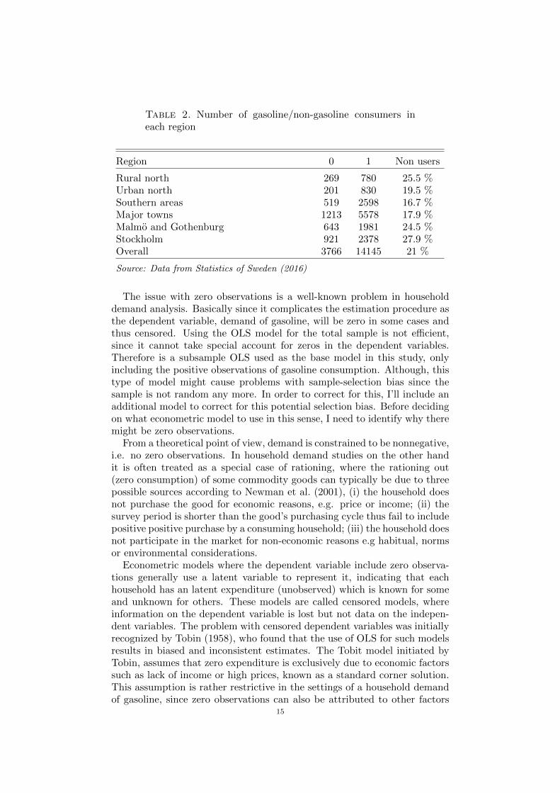
Table 2. Number of gasoline/non-gasoline consumers ineach region

Region 0 1 Non users

Rural north 269 780 25.5 %Urban north 201 830 19.5 %Southern areas 519 2598 16.7 %Major towns 1213 5578 17.9 %Malmo and Gothenburg 643 1981 24.5 %Stockholm 921 2378 27.9 %Overall 3766 14145 21 %

Source: Data from Statistics of Sweden (2016)

The issue with zero observations is a well-known problem in householddemand analysis. Basically since it complicates the estimation procedure asthe dependent variable, demand of gasoline, will be zero in some cases andthus censored. Using the OLS model for the total sample is not efficient,since it cannot take special account for zeros in the dependent variables.Therefore is a subsample OLS used as the base model in this study, onlyincluding the positive observations of gasoline consumption. Although, thistype of model might cause problems with sample-selection bias since thesample is not random any more. In order to correct for this, I’ll include anadditional model to correct for this potential selection bias. Before decidingon what econometric model to use in this sense, I need to identify why theremight be zero observations.

From a theoretical point of view, demand is constrained to be nonnegative,i.e. no zero observations. In household demand studies on the other handit is often treated as a special case of rationing, where the rationing out(zero consumption) of some commodity goods can typically be due to threepossible sources according to Newman et al. (2001), (i) the household doesnot purchase the good for economic reasons, e.g. price or income; (ii) thesurvey period is shorter than the good’s purchasing cycle thus fail to includepositive positive purchase by a consuming household; (iii) the household doesnot participate in the market for non-economic reasons e.g habitual, normsor environmental considerations.

Econometric models where the dependent variable include zero observa-tions generally use a latent variable to represent it, indicating that eachhousehold has an latent expenditure (unobserved) which is known for someand unknown for others. These models are called censored models, whereinformation on the dependent variable is lost but not data on the indepen-dent variables. The problem with censored dependent variables was initiallyrecognized by Tobin (1958), who found that the use of OLS for such modelsresults in biased and inconsistent estimates. The Tobit model initiated byTobin, assumes that zero expenditure is exclusively due to economic factorssuch as lack of income or high prices, known as a standard corner solution.This assumption is rather restrictive in the settings of a household demandof gasoline, since zero observations can also be attributed to other factors

15

such as habitual non-usage, infrequency of travelling or better alternativetransport modes.

To better address this potential bias in the gasoline demand context, theHeckman’s two stage sample selection estimator (Heckman, 1976) has beenwidely used (e.g Blow and Crawford, 1997; Kayser, 2000; West and Williams,2004) and will therefore also be followed in this study.

Heckman’s two stage procedure is specified by a selection equation andan outcome equation. Statistically, the outcome equation is estimated uponthe choice of consuming gasoline (selection equation). This allows to makestatements about how the choice to consume may structurally affect itsconsumption level. Assuming the initial demand equation of gasoline to besummarized in the following way,

lnQi = βi + ηy lnY + ηp lnPi +∑

lnZk ≡ x1β1 + υ1

Then to include the zero observations consistently by the Heckman’s ap-proach, the first stage is to use the selective equation that is estimated as aprobit regression,

g∗i = xδ2 + ν2

where the dependent variable g∗i is a latent variable which takes values zeroor one, where one represent if the household consumes gasoline or alter-natively (e.g Kayser, 2000 and West and Williams, 2004) if the householdowns a car. This regression express the choice of a household to consumeand from the equation the independent variables x are different from thosein the initial demand equation, x1 due to the exclusive restriction. Variablesinfluencing a household to own or not own a car should be different fromthe variables influencing how much quantity of gasoline to purchase. Fromthe selective equation the inverse Mills ratio can be calculated based on theparameter estimates δ2. Then by including the inverse Mills ratio in theinitial regression model we get to the second step known as the outcomeequation,

lnQi = x1β1 + γ1λ(xδ2) + εi

this equation will give consistent estimates of the parameter vector β1, bythe inclusion of λ. A well written description about this method can bestudied further in Heien and Wesseils (1990).

5.2. Potential drawbacks with single equation model. Overall thesingle equation approach is attractive in its simplicity, nonetheless Sadouletand De Janvry (1995) points out some important drawbacks. Primarily thechoice of functional forms of the demand equation and variables to includeis arbitrary. The structure employed are not based on economic theory andusually rely on computational convenience, common sense and interest inspecific elasticity estimates. As a result there are uncertainties on what isactually measured and if the estimates are sufficiently derived from house-hold behaviour. Further concerning the inflexibility of the functional formswhere the elasticities are constant over all values of the exogenous variables.Specifically this might cause inconsistent results when studying gasoline,since consumers are found to have different income elasticities related to

16

their income but also that this elasticity change as income increase. All ofthese shortcomings are considered in the model I intend to use in this study.

Many gasoline household studies use alternative approaches where gaso-line demand is incorporated in the context of consumer production theory.In these studies households’ need for transportation is fulfilled through theutilization of a household’s vehicle stock in which gasoline is used. Thusgasoline demand is employed as derived demand and thus more in line witheconomic theory (Lancaster, 1966). This can be done using the Heckman’stwo stage approach as I intend to do also in this study.

Considering the functional form, a standard linear model will be used butincluding interaction terms to explore impacts from regional features of de-mand of gasoline. Interaction terms have previously been used in householddemand studies (e.g. Archibald and Gillingham, 1980; Rouwendal, 1996;Kayser, 2000; Nicol, 2003), although most of them include a price and in-come interaction term and report variation of price elasticity with respectto income or income groups. This however fails to study differences in priceelasticity between households based on other characteristics than incomelevel. Wadud et al. (2010) acknowledge this shortcomings and use addi-tional interaction terms between price and rural location as well as incomeand rural location. This method will be followed in this thesis.

The main disadvantage of using a single equation model, however, is thatit does not allow for analysing possible complementarity or substitutabilitybetween the various goods comprising the household consumption basket.In order to model this, a complete demand system is required, which isexplained in the next sub section. Although, this method will not be usedin this thesis, primarily for reasons of data limitations. The data at handsimply better suits a standard linear OLS method.

5.3. Demand systems. Demand systems can efficiently include the wholeconsumption basket and therefore require a large amount of detailed data onconsumption as well as prices. In the context of household gasoline consump-tion this method has been used by researchers worldwide (e.g Brannlund andNordstrom, 2004; Nicol, 2003; West and Williams, 2004)

These system of demand equations applied with consumer demand theorywas originally introduced by Stone (1954). Since then, a number of differ-ent specifications and functional forms have been proposed, where one ofthe most examined is the almost ideal demand system (AIDS) which canbe studied further in Deaton and Muellbauer (1980). The benefits of thesesystems are that they are able to take into account the interdependence oflarge numbers of goods in the choices made by consumers. In addition, effi-ciently incorporate the neoclassical assumption of maximizing utility. For autility maximizing consumer, the total expenditure or income y is equal to acost function representing the minimum expenditure necessary to attain themaximum utility level at given prices, c(u, p). This equality can be invertedto yield the indirect utility function, v(p, y) which is the maximum utilitythe consumer can reach for a given income y at given prices p. There aremany ways such a system can be built and they can not easily be comparedsince the interpretation of the elasticities is model specific. Nicol, 2003 indi-cate that while elasticities might change in the same direction as family size

17

in one country, this is not observed in another country. In order for gasolineelasticity estimates to provide guidance for policy makers, this statementimply the importance of actually studying individual countries more preciseas my study intend to do.

6. Model specification

The gasoline demand model examined in this study is first estimatedby using subsample OLS in the log-log linear and static framework. Bysubsample, it means only including households with positive spending ongasoline.

lnQit = β + βe lnEit + βp lnPt +Hi + σt + γj + εit(1)

where Qit is gasoline consumption of household i in year t, Pt is theaggregate real price of gasoline in year t, Eit denote total expenditure ofhousehold i in year t and η the corresponding elasticities. Hi denotes a vectorof household-specific characteristics. σt represent the fixed time effects tocapture the seasonality of gasoline demand and γj represent the regionalfixed effects.

This constant elasticity model, is adopted also in this study since it pro-vide a good fit of the data and further allows for direct comparison withprevious results from the literature. Since the household data is repeatedcross-section we could in principle treat is as a large pooled cross-section.However, this ignores the time dimension and therefore year specific dum-mies will be included to represent the fixed time effects (εt). In additionthere are regional factors that could affect gasoline consumption, thereforedummies representing each region is included to capture the regional fixedeffects (εj).

6.1. Interaction Parameter Model. To accommodate the possibility thathouseholds in different regions have different price or income responses, in-teraction between the price and total expenditure with dummies represent-ing each region will be used. The final model estimated with OLS is thenformally,

lnQit = β0 +J∑j=5

βjDij +T∑t=7

βtDit +

βe +J∑j=5

βejDij

lnEit+(2)

βp +

J∑j=5

βpjDij

lnPt +

K∑k=7

Hi + εit ≡ X′iβ + εit

Dit are the dummy variables of the the different years, Dij are the dummyvariables of household i in region j. Since we include k−1 number of dummyvariables, one of them will be excluded among the regressors and work asthe reference. The parameters β represent the corresponding elasticities forthe variables, besides β0 which is a constant and ε the error term.

The interaction term lnPtDij captures the extent to which the responsive-ness of households to price changes increase or decrease as place of resident

18

changes. In this specification, the price elasticity of gasoline demand foreach region is equal to βpj = βp + βpj , where region one has the price elas-ticity estimate = βp+βp1. Given that the price elasticity is less than zero, apositive coefficient estimate of βpj indicate a decrease in the price responsefor households in the given region. The same interpretation goes for theinteraction lnEtDij .

With the region-year repeated cross-section data at hand, Bertrand et al.(2002) and Kezdi (2003) emphasize that clustering can be present even af-ter including region and year effects in the regression and valid statisticalinference requires controlling for clustering within regions. Failure to do somight lead to under-estimated standard errors and low p-values. A solu-tion is to use cluster-robust standard errors which allows for independenceacross clusters but correlation within clusters. This is convenient for esti-mators to retain their consistency when statistical inference since the usualcross-section assumption of independent observation is no longer appropri-ate (Cameron and Miller, 2015). Even though I also have different timeperiods, the clustering should not be year-region since the error for urbanareas in 2006 is likely to be correlated with the error for urban areas in 2007.

6.2. Heckman selection specification. The second estimation is the Heck-man selection model. This is done in order to correct for possible sampleselection bias from the subsample OLS. First, a probit regression is com-puted that determines the probability that a given household will consumegasoline, where the decision to consume is modelled as a dichotomous choiceproblem. From this regression the inverse Mills ratio (λi) is estimated, whichis included as an instrument in the second stage. The second stage is knownas the outcome equation and is the initial demand model (5), including theλi which incorporates the censoring latent variables to control for the biascaused by non-random sampling.First stage probit regression:

S∗i = αo + α1 ln pi + α2 ln yi + α3TENi +∑k

αkHik + νi ≡ Z′iα+ νi(3)

where S∗ is the unobserved spending on gasoline which is equal to one ifthe household has positive spending on gasoline and equal to zero if not. Hik

is a vector of household characteristics that determine different preferencesin the spending decision on gasoline. TEN is a dummy variable of whetherthe household owns their place of residence of not. Previous theoreticalwork regarding the specification of (6) is limited, Heien and Wesseils (1990)suggest that prices, total expenditure as well as demographic characteristicsshould be of equal importance in the probit model to those expected intraditional demand analysis. However, in order to correctly interpret theparameters in the two equations either the error terms must be uncorrelated,or if not there must be at least one variable in the probit equation that isnot included in the outcome equation (Maddala, 1983).

West (2004), suggest home ownership to be a good alternative since itacts as a proxy for wealth and access to credits and therefore increase thelikelihood of owning a car and thus the likelihood of consuming gasoline,but is not expected to affect quantity of gasoline consumed. In the data

19

I have, there’s no information regarding car ownership. Although, it canbe assumed that households with positive expenditure own or at least haveaccess to a car and therefore it can be used as a proxy for car ownership.Thus, variables that explain car ownership can also be used in this settingsand therefore is home ownership used as the additional variable in the probitregression.

Furthermore, we assume that (νi, εit) has a bivariate normal distributionwith correlation ρ and zero means. Following the specification by Kayser(2000), the expected gasoline demand of (5) become,

E[ln(Qit)|Si > 0] = E[X′iβ + εit|H

′ikα > υi] = X

′iβ + ρσε

φ(Z′iα)

Φ(Z′iα)

where,

φ(Z′iα)

Φ(Z′iα)

is the inverse Mills ration that denotes the non-selection hazard. Lastly thesecond stage outcome equation is expressed,

lnQit = X′iβ + βλλi + εitλ =

φ(Z′iα)

Φ(Z′iα)

(4)

Leung and Yu (1996) points out that the degree of collinearity betweenthe regressors used in the outcome equation and λi is the decisive criteriato judge the appropriateness of the Heckman’s approach in relation to sub-sample OLS. The lack of exclusion restrictions, as in this study, is likely tocause collinearity issues and to test this we follow’s example and estimate λi on all the regressors in the outcome equation.

Following (Kayser, 2000), the short run elasticities can be estimated by,

ηp =∂E[ln(Qi)|Xi]

∂p= β1 + β2

ηy =∂E[ln(Qi)|Xi]

∂y= β2 + β2

7. Results and discussion

Table 3 shows the empirical results from the models estimated in thisthesis. The first column (1) is the initial subsample OLS estimates, thesecond (2) denote the results from the outcome equation of Heckman’s twostage model and (3) the probit regression of Heckman’s model. The numbersin the parenthesis under the coefficient estimate are the standard errors.In the initial subsample OLS (1) these are adjusting for clustering. Theclustering procedure resulted in overall lower standard errors of the estimatesof the parameters.

Since dummy variables are used in the model to represent the differentregions and other demographic characteristics of the household, a referencehousehold is defined. The reference household is headed by a female, with

20

no children and living alone. The household is located in the region definedas ”Major towns”. Interpretation of the variables in table 3 is then donewith respect to this reference household.

The purpose of using the Heckman’s model, was to eliminate problemswith selection bias by including the inverse Mills ratio in the gasoline de-mand (outcome) equation. Although, since the Mills ratio,λ, is significant itmeans we have high correlation between the error terms of the two modelsand the problem with selection bias is not solved. Regressing λ on all thevariables in the outcome equation result in highly significant parameters andadjusted R2 of 0.89, which imply problems with collinearity. The problemwith collinearity in this study is most likely related to that only one addi-tional variable, home ownership, is included in the selection model and/orthat home ownership also explains the quantity of gasoline consumed.

In order to correct for collinearity, the standard procedure is to find moreappropriate exclusive restrictions. That is, find variables that determinethe probability to consume gasoline, but do not determine the quantityconsumed directly. Two examples could be distance to work or if holding adriver license. Puhani (2000) suggest if there are problems with collinearityin the Heckman’s procedure that can not be solved, subsample OLS may bethe most robust estimator. Due to problem with collinearity connected tothe Heckman’s approach, and the lack of possibilities to reduce collinearitywith the data at hand, from now on I’ll only focus on the estimates frominitial subsample OLS (1) since this model is assumed to be the most robustalternative.

First looking at the household characteristics, the male variable is signif-icant and positive, which indicate that households where male is the headof household have a positive influence on demand of gasoline. This findingis well-supported in the literature. Carlsson-Kanyama and Linden (1999)studies 45 000 individuals in Sweden and confirm that men with high in-come are the most intensive users of car fuel. Since a dummy variable isnot a continuous variable, we can not interpret the parameter estimate asthe marginal effect of log of demands. Instead Halvorsen et al. (1980) showthat the percentage change of a dummy variable is given by eβ − 1 where βis the coefficient estimate of the dummy. In this case, households with malehead consume 14.8 percent more gasoline than those with female head.

Age of household head is significant and have expected signs as the ageof household head has a positive influence on gasoline demand, while thenegative sign of age squared means that as the head of household gets older,the effect of age is lessoned. The more adults and children there are in thehousehold have a significant positive effect on gasoline consumption, whichis consistent to results by West and Williams (2004).

Turning over to the research question of this study, which questioned ifthere are potential differences between the gasoline elasticities of demandin rural and urban regions in Sweden. In table 3 we first find that thepositive statistically significant coefficient of the interaction term betweenprice and rural north establish that gasoline demand for households in therural areas are less price elastic than households in major towns. This finding

21

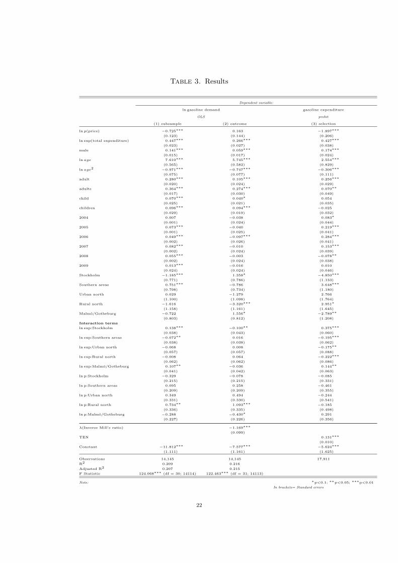
Table 3. Results

Dependent variable:

ln gasoline demand gasoline expenditure

OLS probit

(1) subsample (2) outcome (3) selection

ln p(price) −0.725∗∗∗ 0.163 −1.897∗∗∗

(0.123) (0.144) (0.206)

ln exp(total expenditure) 0.447∗∗∗ 0.266∗∗∗ 0.427∗∗∗

(0.023) (0.027) (0.038)

male 0.141∗∗∗ 0.059∗∗∗ 0.174∗∗∗

(0.015) (0.017) (0.024)

ln age 7.610∗∗∗ 5.745∗∗∗ 2.554∗∗∗

(0.565) (0.582) (0.829)

ln age2 −0.971∗∗∗ −0.747∗∗∗ −0.306∗∗∗

(0.075) (0.077) (0.111)

adult 0.280∗∗∗ 0.105∗∗∗ 0.256∗∗∗

(0.020) (0.024) (0.029)

adults 0.364∗∗∗ 0.274∗∗∗ 0.070∗∗

(0.017) (0.030) (0.049)

child 0.070∗∗∗ 0.040∗ 0.054

(0.025) (0.021) (0.035)

children 0.096∗∗∗ 0.094∗∗∗ −0.025

(0.029) (0.019) (0.032)

2004 0.007 −0.038 0.083∗

(0.001) (0.024) (0.044)

2005 0.073∗∗∗ −0.040 0.219∗∗∗

(0.001) (0.025) (0.041)

2006 0.049∗∗∗ −0.097∗∗∗ 0.284∗∗∗

(0.002) (0.026) (0.041)

2007 0.082∗∗∗ −0.010 0.153∗∗∗

(0.002) (0.024) (0.039)

2008 0.055∗∗∗ −0.003 −0.078∗∗

(0.002) (0.024) (0.038)

2009 0.013∗∗∗ −0.016 0.010

(0.024) (0.024) (0.046)

Stockholm −1.185∗∗∗ 1.358∗ −4.850∗∗∗

(0.771) (0.786) (1.133)

Southern areas 0.751∗∗∗ −0.786 3.648∗∗∗

(0.798) (0.734) (1.180)

Urban north 0.029 −1.279 2.766

(1.100) (1.098) (1.764)

Rural north −1.616 −3.320∗∗∗ 2.951∗

(1.158) (1.161) (1.645)

Malmo/Gotheburg −0.722 1.556∗ −2.789∗∗

(0.803) (0.812) (1.208)

Interaction terms

ln exp:Stockholm 0.138∗∗∗ −0.100∗∗ 0.375∗∗∗

(0.038) (0.043) (0.060)

ln exp:Southern areas −0.072∗∗ 0.016 −0.195∗∗∗

(0.038) (0.038) (0.062)

ln exp:Urban north −0.068 0.008 −0.175∗∗

(0.057) (0.057) (0.088)

ln exp:Rural north −0.008 0.064 −0.222∗∗∗

(0.062) (0.062) (0.086)

ln exp:Malmo/Gotheburg 0.107∗∗ −0.036 0.144∗∗

(0.041) (0.042) (0.063)

ln p:Stockholm −0.329 −0.078 −0.085

(0.215) (0.215) (0.331)

ln p:Southern areas 0.095 0.258 −0.461

(0.209) (0.209) (0.355)

ln p:Urban north 0.349 0.494 −0.244

(0.331) (0.330) (0.541)

ln p:Rural north 0.734∗∗ 1.093∗∗∗ −0.185

(0.336) (0.335) (0.498)

ln p:Malmo/Gotheburg −0.288 −0.430∗ 0.291

(0.227) (0.226) (0.356)

λ(Inverse Mill’s ratio) −1.169∗∗∗

(0.099)

TEN 0.131∗∗∗

(0.010)

Constant −11.812∗∗∗ −7.577∗∗∗ −5.624∗∗∗

(1.111) (1.161) (1.625)

Observations 14,145 14,145 17,911

R2 0.209 0.216

Adjusted R2 0.207 0.215

F Statistic 124.068∗∗∗ (df = 30; 14114) 122.463∗∗∗ (df = 31; 14113)

Note: ∗p<0.1; ∗∗p<0.05; ∗∗∗p<0.01

In brackets= Standard errors

22

is consistent with similar studies in the UK by Blow and Crawford (1997)and Santos and Catchesides (2005).

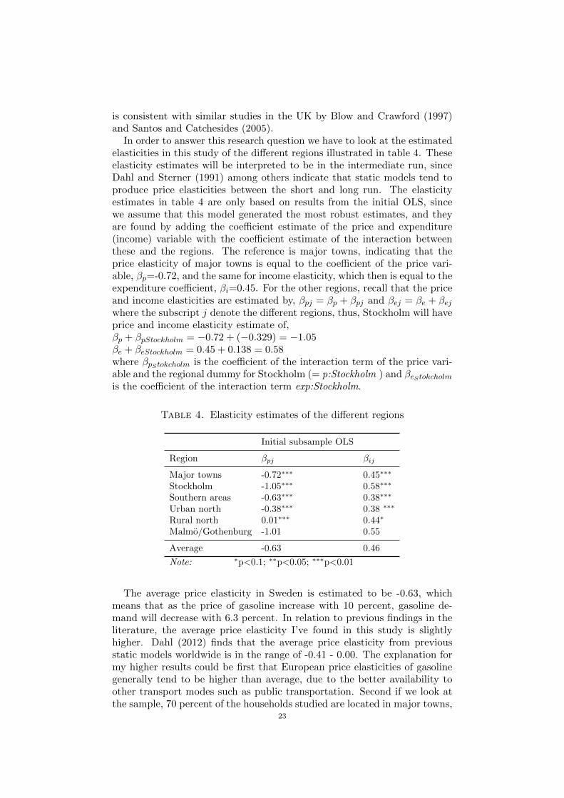
In order to answer this research question we have to look at the estimatedelasticities in this study of the different regions illustrated in table 4. Theseelasticity estimates will be interpreted to be in the intermediate run, sinceDahl and Sterner (1991) among others indicate that static models tend toproduce price elasticities between the short and long run. The elasticityestimates in table 4 are only based on results from the initial OLS, sincewe assume that this model generated the most robust estimates, and theyare found by adding the coefficient estimate of the price and expenditure(income) variable with the coefficient estimate of the interaction betweenthese and the regions. The reference is major towns, indicating that theprice elasticity of major towns is equal to the coefficient of the price vari-able, βp=-0.72, and the same for income elasticity, which then is equal to theexpenditure coefficient, βi=0.45. For the other regions, recall that the priceand income elasticities are estimated by, βpj = βp + βpj and βej = βe + βejwhere the subscript j denote the different regions, thus, Stockholm will haveprice and income elasticity estimate of,βp + βpStockholm = −0.72 + (−0.329) = −1.05βe + βeStockholm = 0.45 + 0.138 = 0.58where βpStokcholm is the coefficient of the interaction term of the price vari-able and the regional dummy for Stockholm (= p:Stockholm ) and βeStokcholmis the coefficient of the interaction term exp:Stockholm.

Table 4. Elasticity estimates of the different regions

Initial subsample OLS

Region βpj βij

Major towns -0.72∗∗∗ 0.45∗∗∗

Stockholm -1.05∗∗∗ 0.58∗∗∗

Southern areas -0.63∗∗∗ 0.38∗∗∗

Urban north -0.38∗∗∗ 0.38 ∗∗∗

Rural north 0.01∗∗∗ 0.44∗

Malmo/Gothenburg -1.01 0.55

Average -0.63 0.46

Note: ∗p<0.1; ∗∗p<0.05; ∗∗∗p<0.01

The average price elasticity in Sweden is estimated to be -0.63, whichmeans that as the price of gasoline increase with 10 percent, gasoline de-mand will decrease with 6.3 percent. In relation to previous findings in theliterature, the average price elasticity I’ve found in this study is slightlyhigher. Dahl (2012) finds that the average price elasticity from previousstatic models worldwide is in the range of -0.41 - 0.00. The explanation formy higher results could be first that European price elasticities of gasolinegenerally tend to be higher than average, due to the better availability toother transport modes such as public transportation. Second if we look atthe sample, 70 percent of the households studied are located in major towns,

23

Stockholm and Malmo/Gothenburg, all areas in which alternative transportto car transport for sure is an alternative.

With respect to the different regional elasticity estimates, all are signif-icant but Malmo/Gothenburg. The overall pattern of the price elasticitiesillustrate that the rural region is inelastic and Stockholm is very elastic. Asimilar pattern is found by Bureau (2011) in France and Santos and Catche-sides (2005) in the UK, where the rural region seem to be less responsive toprice changes and urban areas on the other hand are more responsive. AlsoNicol (2003), find regional differences of price elasticities to vary between-0.103 and -0.894 in Canada.

The reason why the regional price elasticities are different could be thathouseholds in rural regions for instance tend to keep their car longer andthus their car stock turns over to efficient vehicles more slowly and thereforelowering their price responsiveness. This is also connected to infrastructuralissues, where it in rural areas might not be possible to switch to vehiclesdriven by alternative fuels since there might, for instance, be limited placesto charge an electric car. Also, infrastructural issues in terms of publictransportation, which is less developed in rural areas and thus decrease theopportunity to substitute between different modes of transport.

In table 4 it’s shown that the urban north price elasticity is -0.38 comparedto southern areas of -0.68 , which is quite interesting if the reasoning thataccess public transportation might have influence on the price elasticity.In this case the urban north should in principal be more price responsivethan southern areas since it is not defined as an urban area, but this is notthe case. One explanation for this could be that work and home may befurther apart in the northern regions, thus, even if there are better publictransportation these transits are not suitable to fit the travelling behaviourof the households. Another reason could be related to cultural differences,where it’s more accepted to use other types of transport than a car in thesouthern areas compared to in the northern region.

Even though the general pattern of the price elasticity estimates found inthis study are similar to those reported by others, it is possible that they aremisspecified which may lead to inconsistent estimators whose the propertiesare unknown (Blundell et al., 2012). In the rural north for instance, theprice elasticity is estimated to be almost perfectly inelastic at 0.01, whichindicate that as the price of gasoline increase with 10 percent, the demandof gasoline will be almost unchanged or slightly go up. This might be due tothat households in these areas face higher prices in the real world, comparedto the annual average gasoline price in Sweden used as the price variable inthis thesis. Using a constant price variable is problematic when analysingregional effects, and is used in this study mainly because of data limitationsof regional gasoline prices. The best solution for this would be to find moredetailed price data and then apply a non parametric estimator to be sure tofind consistent estimates, i.e. use a system of demand model instead of thelinear single equation. An alternative solution may have been to drop theprice variable from the estimation and use an expenditure function insteadof a demand equation. Thus, in this case I would not have found any priceelasticity estimates of the different regions but only the income elasticities.

24

Turning to the income elasticity estimates in table 4, the average is 0.46which is in line with previous studies. Dahl (2012) finds that the average in-come elasticity is between 0.00-0.53.The income elasticity estimates are morereliable compared to the price elasticity, since these are based on the house-holds individual total expenditure and therefore more precise compared tothe average price variable. However, the various income elasticity estimatesof the regions are positive and below one, thus, gasoline seem to be a normalgood in all regions. In addition the elasticity estimates do not change muchbetween the regions, which is also found by Blow and Crawford (1997) andWadud et al. (2010). Therefore we can conclude that the regional dimensionin terms of income elasticity is not very strong. More specifically, however,Stockholm has an income price elasticity of 0.58, which indicate that as in-come increase with 10 percent, gasoline demand increase with 5.8 percent.Where the rural north on the other hand has an income elasticity of 0.44,which imply that as income increase with 10 percent, gasoline demand in-crease with 4.4 percent. Although the difference is quite small these resultsstress that the income effect is slightly stronger in Stockholm, which meansthat as income for households in Stockholm increase they will demand moregasoline compared to if income would rise with the same percentage sharefor households in the rural region.

Finally, in order to see the overall how well the subsample OLS preformand if its results is trustful, first we can turn to the standard adjustedR2. In this model it’s 20.9 percent, which means that the independentvariables explain 20.9 percent of the variation in the dependent variable.This might be a low result, however the adjusted R2 is not the final answerwhether the model preform well or not since it does not provide a formalhypothesis test for the relationship between the independent and dependentvariables. For this we need to do an F-test. The F-test provides a test ofthe overall significance. It compares an intercept only model with the modelspecified (subsample OLS). The null hypothesis for the F-test is that there’sno relationship between quantity of gasoline demanded and the independentvariables. The overall F-test is significant and therefore the null hypothesisis rejected and the subsample OLS model is expected to provide a better fitthan the intercept only model.

8. Conclusion

In this thesis the aim has been to investigate the potential differences ofgasoline demand elasticities in different regions in Sweden, using the staticlog-log linear OLS method and Swedish Household budget data between2003-2006 and 2012. The results show that the regional differences in termsof price elasticity of gasoline seems to vary more distinct in comparison tothe income elasticity.

Thus, the increased fuel tax initiated by the Swedish government willtrigger different responses in households living in different regions. Giventhe price elasticity estimates, northern households will carry a greater shareof the financial burden of the tax, especially the rural ones. In Stockholm,Gothenburg and Malmo on the other hand the tax increase might be veryefficient in reducing demand of gasoline since the price elasticity is elastic.

25

This means that if there is a political will to equalize the distributional ef-fects, households in rural areas should be compensated. Lower fuel taxes inthese areas might not necessarily be favoured though, since differentiationwould kill the incentive to restrict gasoline consumption. The distributionalimpacts from a tax increase should rather be handled by recycling the rev-enues efficiently.

In addition, it should be remembered that the model presented here isbased on estimates in the intermediate-run. In the long-run, householdscan adapt their travelling behaviour in response to higher gasoline taxes byswitching to a more fuel efficient car or using alternative transport modes.In this case the distributive effect of a tax reform will be reduced. Although,this is very hard to test, since it will depend on future infrastructural changesspecifically relevant in the rural areas.

8.1. Ethical considerations. Two ethical dimensions can be related tothis study. First, with respect to the regional location of the household withthe ethical perspective of the direct welfare effects connected to the regions.Second, as the goal of the environmental tax to reduce carbon emissionsfrom private car travelling, thus take responsibility for the welfare of futuregenerations.

The sometimes troublesome dilemma of an environmental tax, where it’sin theory is justified to tax those who bear the burden of negative externaleffects as long as the social cost exceeds the cost of the tax. However, ifthose most economically punished by the tax, such as rural households inthis study, are so for reasons out of their reach the environmental tax mightnot be justified in reality. The environmental fuel tax with the goal tochange behaviour to decrease carbon emissions, is not ethical in the sensethat rural households don’t have the same ability to change their behaviouras the urban households. This study aim to highlight the importance ofevaluating behavioural changes in order to actually reach the goal of anenvironmental fuel tax policy.

In the long run, on the other hand, there’s an ethical responsibility forfuture generations. The transport sector has an overall increasing trend ofcarbon emissions. What is really needed is to clarify how we should transportourselves in the future since the current situation is not sustainable. If afuel tax can assist financially to develop a future strategy then the unequalwelfare changes today might not be as relevant.

8.2. Future studies. Future research with more detailed price data onregional level using a more sophisticated system of demand approach wouldbe interesting to see with respect to specific elasticity estimates. In additiona more in depth study on why rural regions seem to respond to less to pricechanges and what is actually needed to change behaviour in terms of drivingless or more efficient. More relevant research is needed on a sub-nationallevel of the transport sector.

26

References

Akerman, J., Banister, D., Dreborg, K., Nijkamp, P., Schleicher-Tappeser,R., Stead, D., Steen, P., 2000. European transport policy and sustainablemobility. Routledge.

Archibald, R., Gillingham, R., 1980. An analysis of the short-run consumerdemand for gasoline using household survey data. The Review of Econom-ics and Statistics, 622–628.

Becker, G. S., 1965. A theory of the allocation of time. The economic journal75 (299), 493–517.

Bento, A. M., Goulder, L. H., Jacobsen, M. R., Von Haefen, R. H., 2009.Distributional and efficiency impacts of increased us gasoline taxes. TheAmerican Economic Review, 667–699.

Bertrand, M., Duflo, E., Mullainathan, S., 2002. How much should we trustdifferences-in-differences estimates? Tech. rep., National Bureau of Eco-nomic Research.

Blow, L., Crawford, I., 1997. The distributional effects of taxes on privatemotoring.

Blundell, R., Horowitz, J. L., Parey, M., 2012. Measuring the price respon-siveness of gasoline demand: Economic shape restrictions and nonpara-metric demand estimation. Quantitative Economics 3 (1), 29–51.

Brannlund, R., Nordstrom, J., 2004. Carbon tax simulations using a house-hold demand model. European Economic Review 48 (1), 211–233.

Bureau, B., 2011. Distributional effects of a carbon tax on car fuels in france.Energy Economics 33 (1), 121–130.

Cameron, A. C., Miller, D. L., 2015. A practitioner’s guide to cluster-robustinference. Journal of Human Resources 50 (2), 317–372.

Carlsson-Kanyama, A., Linden, A.-L., 1999. Travel patterns and environ-mental effects now and in the future:: implications of differences in energyconsumption among socio-economic groups. Ecological Economics 30 (3),405–417.

Council of the European Union, 2003. Council directive 2003/96/ec of 27october 2003 restructuring the community framework for the taxation ofenergy products and electricity. Official Journal of the European UnionL283.

Council of the European Union, 2009. Regulation (ec) no 443/2009/ec of theeuropean parliament and of the council of 23 april 2009 setting emissionperformance standards for new passenger cars as part of the community’sintegrated approach to reduce co 2 emissions from light-duty vehicles.Official Journal of the European Union L140.

Dahl, C., Sterner, T., 1991. Analysing gasoline demand elasticities: a survey.Energy economics 13 (3), 203–210.

Dahl, C. A., 2012. Measuring global gasoline and diesel price and incomeelasticities. Energy Policy 41, 2–13.

De Jong, G., Gunn, H., 2001. Recent evidence on car cost and time elas-ticities of travel demand in europe. Journal of Transport Economics andPolicy, 137–160.

Deaton, A., Muellbauer, J., 1980. An almost ideal demand system. TheAmerican economic review 70 (3), 312–326.

27

Eliasson, J., Pyddoke, R., Swardh, J.-E., et al., 2016. Distributional effectsof taxes on car fuel, use, ownership and purchases. Tech. rep., CTS-Centrefor Transport Studies Stockholm (KTH and VTI).

Espey, M., 1998. Gasoline demand revisited: an international meta-analysisof elasticities. Energy Economics 20 (3), 273–295.

European Commission, et al., 2011. Roadmap to a single european transportarea-towards a competitive and resource efficient transport system. WhitePaper, Communication 144.

Friedman, M., 1957. A theory of the consumption function. Vol. 63. JSTOR.Frondel, M., Vance, C., 2013. Fuel taxes versus efficiency standards–an in-

strumental variable approach. Ruhr Economic Paper (445).Halvorsen, R., Palmquist, R., et al., 1980. The interpretation of dummy

variables in semilogarithmic equations. American economic review 70 (3),474–75.

Heckman, J., 1976. The common structure of statistical models of trun-cation, sample selection and limited dependent variables and a simpleestimator for such models.

Heien, D., Wesseils, C. R., 1990. Demand systems estimation with micro-data: a censored regression approach. Journal of Business & EconomicStatistics 8 (3), 365–371.

Houthakker, H. S., Verleger, P. K., Sheehan, D. P., 1974. Dynamic demandanalyses for gasoline and residential electricity. American Journal of Agri-cultural Economics 56 (2), 412–418.

Hughes, J. E., Knittel, C. R., Sperling, D., 2008. Evidence of a shift inthe short-run price elasticity of gasoline demand. The Energy Journal,113–134.

IPCC, 2015. Climate Change 2014: Mitigation of Climate Change. Vol. 3.Cambridge University Press.

Kayser, H. A., 2000. Gasoline demand and car choice: estimating gasolinedemand using household information. Energy economics 22 (3), 331–348.

Kezdi, G., 2003. Robust standard error estimation in fixed-effects panelmodels. Available at SSRN 596988.

Lancaster, K. J., 1966. A new approach to consumer theory. The journal ofpolitical economy, 132–157.

Leung, S. F., Yu, S., 1996. On the choice between sample selection andtwo-part models. Journal of econometrics 72 (1), 197–229.

Liu, W., 2015. Gasoline taxes or efficiency standards? a heterogeneoushousehold demand analysis. Energy Policy 80, 54–64.

Maddala, G., 1983. Qualitative and limited dependent variable models ineconometrics. Cambridge: Cambridge University Press.

Mas-Colell, A., Whinston, M. D., Green, J. R., et al., 1995. Microeconomictheory. Vol. 1. Oxford university press New York.

Newman, C., Henchion, M., Matthews, A., 2001. Infrequency of purchaseand double-hurdle models of irish households’ meat expenditure. Euro-pean Review of Agricultural Economics 28 (4), 393–419.

Nicol, C. J., 2003. Elasticities of demand for gasoline in canada and theunited states. Energy economics 25 (2), 201–214.

28

Pollak, R. A., Wales, T. J., et al., 1995. Demand system specification andestimation. OUP Catalogue.

Poterba, J. M., 1991. Is the gasoline tax regressive? Tax Policy and theEconomy, 145–164.

Proost, S., Van Dender, K., 2011. What long-term road transport future?trends and policy options. Review of Environmental Economics and Policy5 (1), 44–65.

Puhani, P., 2000. The heckman correction for sample selection and its cri-tique. Journal of economic surveys 14 (1), 53–68.

Puller, S. L., Greening, L. A., 1999. Household adjustment to gasoline pricechange: an analysis using 9 years of us survey data. Energy Economics21 (1), 37–52.

Rouwendal, J., 1996. An economic analysis of fuel use per kilometre byprivate cars. Journal of Transport Economics and Policy, 3–14.

Sadoulet, E., De Janvry, A., 1995. Quantitative development policy analysis.No. 338.9011 S3. Johns Hopkins University Press Baltimore.

Santos, G., Catchesides, T., 2005. Distributional consequences of gasolinetaxation in the united kingdom. Transportation Research Record: Journalof the Transportation Research Board (1924), 103–111.

Sperling, D., Nichols, M., 2012. California’s pioneering transportation strat-egy. Issues in Science and Technology 28 (2), 59.

Statistics of Sweden, 2016. Household expenditure. Accessed on 2016-06-01.URL http : / / www . scb . se / sv _ /Hitta-statistik /

Statistik-efter-amne/Hushallens-ekonomi/Hushallens-utgifter/

Hushallens-utgifter-HUT/

Stern, N., 2007. The economics of climate change: the Stern review. cam-bridge University press.

Stock, J. H., Watson, M. W., 2012. Introduction to econometrics. PearsonEducation.

Stone, R., 1954. Linear expenditure systems and demand analysis: an appli-cation to the pattern of british demand. The Economic Journal 64 (255),511–527.

Swedish Petroleum and Biofuels Institute, 2016. Gasoline price and con-sumption. Accessed on 2016-06-01.URL ttp://spbi.se/statistik/priser/bensin/

The Swedish Government, 2015. The government budget propsition2015/16:1.

Tobin, J., 1958. Estimation of relationships for limited dependent variables.Econometrica: journal of the Econometric Society, 24–36.

Van Dender, K., 2009. Energy policy in transport and transport policy.Energy Policy 37 (10), 3854–3862.

Verbeek, M., 2008. A guide to modern econometrics. John Wiley & Sons.Wadud, Z., Graham, D. J., Noland, R. B., 2010. Gasoline demand with

heterogeneity in household responses. The Energy Journal, 47–74.Wales, T. J., Woodland, A. D., 1983. Estimation of consumer demand sys-

tems with binding non-negativity constraints. Journal of Econometrics21 (3), 263–285.

29

West, S. E., 2004. Distributional effects of alternative vehicle pollution con-trol policies. Journal of public Economics 88 (3), 735–757.

West, S. E., Williams, R. C., 2004. Estimates from a consumer demandsystem: implications for the incidence of environmental taxes. Journal ofEnvironmental Economics and management 47 (3), 535–558.

30

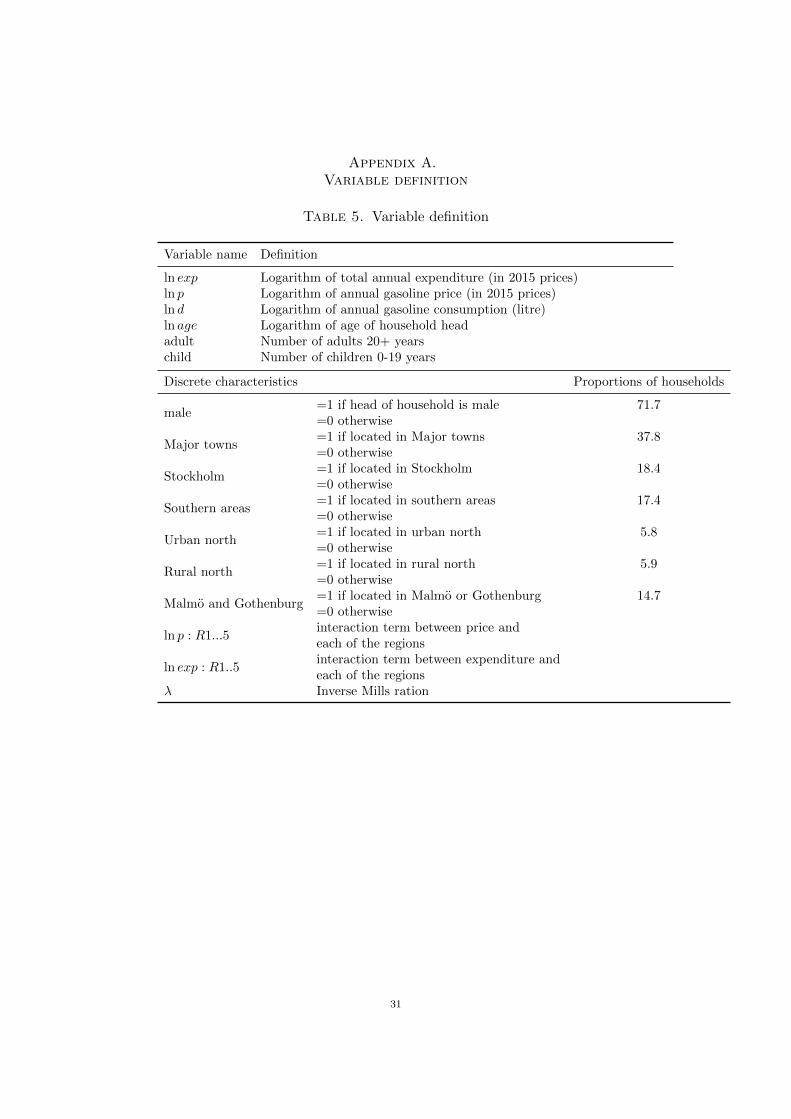
Appendix A.Variable definition

Table 5. Variable definition

Variable name Definition

ln exp Logarithm of total annual expenditure (in 2015 prices)ln p Logarithm of annual gasoline price (in 2015 prices)ln d Logarithm of annual gasoline consumption (litre)ln age Logarithm of age of household headadult Number of adults 20+ yearschild Number of children 0-19 years

Discrete characteristics Proportions of households

male=1 if head of household is male 71.7=0 otherwise

Major towns=1 if located in Major towns 37.8=0 otherwise

Stockholm=1 if located in Stockholm 18.4=0 otherwise

Southern areas=1 if located in southern areas 17.4=0 otherwise

Urban north=1 if located in urban north 5.8=0 otherwise

Rural north=1 if located in rural north 5.9=0 otherwise

Malmo and Gothenburg=1 if located in Malmo or Gothenburg 14.7=0 otherwise

ln p : R1...5interaction term between price andeach of the regions

ln exp : R1..5interaction term between expenditure andeach of the regions

λ Inverse Mills ration

31