The effects of the Dot Com bubble and the Credit Crisis on

leverage ratios of US non-financial firms

Name: N.T. Joosten

ANR: 194352

Defense date: October 25, 2012

Supervisor: Dr. F. Braggion

Chairman: Dr. P. De Goeij

Master Thesis Finance, Tilburg University

Tilburg School of Economic and Management

Word Count: 17193

1

The effects of the Dot Com bubble and the Credit Crisis on leverage

ratios of US non-financial firms

Nico Theodoor Joosten

Master Thesis Finance, Tilburg University

TiSEM: Tilburg School of Economic and Management PO Box 90153, NL 5000 LE Tilburg, The Netherlands

Supervisor:

dr. F. Braggion

TiSEM: Department of Finance PO Box 90153, NL 5000 LE Tilburg, The Netherlands

Abstract

This thesis researches the impact of the Dot Com bubble and the Credit Crisis on the leverage of US non-

financial firms, over the period 1995-2011. The data consists of 24,600 US firms. The research is done

using the main determinants of leverage and the existing Capital Structure Theories. The aim of this

research is trying to give a fresh insight in the effects of the Dot Com bubble and the Credit Crisis on

leverage ratio of US non-financial firms. The main results are: the ‘initial’ determinants of leverage work

to explain the leverage ratio of US non-financial Firms during a crisis. Furthermore they also seem to

explain the effects of both of the crises over the period 1995-2011. The Capital Structure theories seem

to hold during periods of distress. The circumstances caused by the Dot Com have large influence on the

effects on leverage during the Credit Crisis. Finally the system does not seem to be in a new ‘optimum’

boundary after the Credit Crisis, but lack of data availability makes this hard to conclude.

Key words: Capital Structure, Leverage, Dot Com Bubble, Credit Crisis

JEL Codes: G01, G18, G32

2

Acknowledgements

This Thesis is the final part of my Master Finance at Tilburg University. The aim of this research is to

combine what I have learned in the past years and to give a fresh insight in firms leverage ratios over a

long period of time. This is the final product and of my years at Tilburg University. It also marks the end

of my life as a student in Tilburg.

I would like to take this opportunity to express my thanks to some people. First of all I would like to

thank my supervisor Dr. F. Braggion for his advice. He helped me with providing adequate advice and

new insights needed to complete this thesis. Second I would like to thank Dr. P. de Goeij, for reading my

thesis and being chairman of the exam committee. Further, I would like to thank my mother Mieke,

girlfriend Sanne and my brother Bas for their support and patience they had with me during my entire

study in Tilburg. Finally I would like to thank my friends, family and roommates for the support and the

pleasant times we had next to studying.

3

Table of Contents

Abstract 1

Acknowledgements 2

Section 1: Intro 4

Section 2: Crises 7

2.1 Other crisis and important events 7

2.2 Dot Com bubble 10

2.3 Credit Crisis 12

2.4 Differences and similarities between the Dot Com and the Credit Crisis 16

Section 3: Literature 17

Section 4: Hypothesis, Data and Methodology 27

4.1 Hypothesis 27

4.2 Data and Sample Selection 28

4.3 Methodology 29

4.4 Outliers 31

4.5 Variables 32

4.6 Correlation Matrix 37

Section 5: Results 38

Section 6: Conclusion and recommendations 50

REFERENCES 53

APPENDICES 58

4

Section 1: Intro

The fall of Lehman Brothers in 2008 is probably the major event that introduced the Credit Crisis to a big

audience. Different events and circumstances before the crisis piled up to what eventually turned out to

be the Credit Crisis. The effects of this crisis are still visible worldwide and the severity of this crisis is

only matched by the Great Depression of the 1930s. The Credit Crisis is the second big crisis in this

millennium. The first one is the Dot Com bubble. This is named after the web-based companies, which

were the cause of the bubble. This research will cover them both.

The fact that the Asian Crisis (1997) did not lead to a worldwide contagion and the little contagion of the

Dot Com bubble led to the belief that a crisis, like the Credit Crisis, could be controlled without

contagion to other industries. At this point in time we know better. The Credit Crisis did not happen

overnight, but it was a buildup of different events and regulation changes over a long period of time that

created a contaminated environment. They eventually resulted into the burst, with as a major cause the

Dot Com bubble and its aftermath. In the beginning of the crisis the housing bubble, along with the

Mortgage Backed Securities (MBS), collapsed and spread out through the rest of the financial markets

and then the entire economy. This along with regulation changes and government and Fed polices, new

innovative financial products, created the entire shortfall in the US economy and the fall of some big

companies.

Where the Dot Com bubble occurred in a one new industry, the credit crisis started out in an existing

one. Since legislative changes in the aftermath of the Dot Com bubble created the circumstances for the

Credit Crisis. In order to get a more clear insight in the Credit Crisis, it is wise to compare the two crises

and look if there were similarities and differences in what created them and if the effects of the Dot

Com bubble really created the Credit Crisis. So the aim of this research is to give a fresh insight in both

the Dot Com bubble and the Credit Crisis and their effects on firms’ leverage. Previous research shows

5

ambiguous findings in the effects of a crisis on a firm’s leverage. The findings are counter-cyclical, pro-

cyclical and or showed no effect (static over time). These different results open opportunities to

investigate the effect of the crises on firms as well as the entire economy. Where most research

investigates the effect of the Credit Crisis on either US financials or the effects on non-US countries, the

aim of my research is to get an insight in the impact on firms’ leverage ratio over long period with two

crises on the US economy, more specific non-financial US firms. Therefore the main research question

will be:

What are the effects of the Dot Com bubble and the Credit Crisis on leverage ratios of US non-financial

firms?

This research will cover all US non-financial firms over the period 1995-2011. This opens opportunities to

investigate both the Dot Com bubble and the Credit Crisis. This period further allows comparison

between the two periods and the effect of the Dot Com bubble on the Credit Crisis. The so-called

determinants of leverage will be used to investigate the Capital Structure theories. Since the Capital

Structure theories are applicable in every crisis and over countries (Booth, Avaizian, Demirguc-Kunt and

Maksimovic, 2001), the results of this research can be used as comparison. The aftermath of the Dot

Com bubble determined the leverage ratios in advance of the Credit Crisis. This will also be examined.

Furthermore a comparison is made between non-financial and financial firms.

As we know now the Credit Crisis was severe and did have major impact on firms and the entire

economy. So it is expected that changes in leverage will show up and the Capital Structure theories and

previously published literature will partly hold, since previous research shows ambiguous results in the

direction of leverage during periods of distress. The only problem in determining the outcome of

leverage after a crisis is that the data availability only allows covering the aftermath of the Dot Com

bubble and not the Credit Crisis, since there are too little year observations after the Credit Crisis.

6

The main findings of this research are that there is a large effect from the crises on leverage.

Furthermore, the initial determinants of leverage work to explain the leverage ratio of US non-financial

Firms. Furthermore they also seem to explain the long-term effects of both of the crises over the period

1995-2011. The Capital Structure theories seem to hold during periods of distress. The shock of the Dot

Com bubble creates effects still noticeable in advance of the Credit Crisis. The results show sharp

inclines of leverage in advance of the crises (mainly the Credit Crisis), followed by a large drop during

both of the crises. Finally the system does not seem to be in a new ‘optimum’ boundary after the Credit

Crisis, but lack of data availability makes this hard to conclude. Furthermore the adding of extra

variables on the base model by further empirical work gives a more profound and robust model in

determining leverage during 1995-2011. Mainly the results found in analysis using Altman’s Z-score

(Altman, 1968). Furthermore the circumstances created by earlier events (and crises) and the reaction of

the governments on them created a contaminated environment for the Credit Crisis. The results of

analyzing Altman’s Z-score show that during the Dot Com bubble Z-score dropped and remained low

(graph 7 appendix).

This research is build up in the following way: the next section starts with a summary of past crises

worth discussing, followed by a discussion of the Dot Com bubble and the Credit Crisis. It ends with a

comparison between the two crises. Section 3 discusses the theory and literature that is relevant for this

research. Based on the literature the next section (4) discusses the hypothesis and methodology. This

section also includes an explanation variables used for the analysis. Section 5 discusses the results and

connects these results to the discussed literature and hypotheses. In the final section (6) the conclusion

are discussed. Furthermore this section addresses the limitations and recommendations of this research

and is ended with some concluding remarks. The results of the analysis can be found in the appendices.

7

Section 2: Crises

In this section I will discuss the main important crises and events that have influence on the Dot Com

bubble, the Credit Crisis or perhaps are at the cause of them. The next step is to discuss the Dot Com

bubble, followed by the 2007 Credit Crisis. Finally the similarities and differences between the two crises

are addressed.

2.1 Other crisis and important events

This research stretches out to investigate the effects of the Dot Com bubble and 2007 Credit Crisis on a

firms’ leverage ratio. Just discussing this timeframe however is not sufficient. First a definition of a crisis

needs to be discussed. After the definition of a crisis and a bubble several important events will be

discussed which are important to give a more profound background for the circumstances during the

Dot Com bubble and the Credit Crisis.

An economic crisis is an unexpected shock in supply or demand with large effects throughout the

economy of financial system (Shiller, 2005) One of the most famous and considered to be the first

‘economic bubble’ is the Dutch Tulip Mania of 1673. This bubble is a sudden bust after a period of boom

in (commodity) prices. So after the price of a certain product rises, it then suddenly falls. The Tulip mania

happened in Holland during its Golden Age. Tulip bulbs were sold for over 10 times the annual income of

craftsman before the market collapsed.

The Great Depression of the 1930s is largest of its kind and had the largest effect on the global economy.

This crisis started on Black Tuesday (October 29, 1929) with the worldwide news of the stock market

crash. During the period after Black Tuesday unemployment rose by 60 percent and international trade

fell. Roosevelt’s New Deal policy was set up to make a recovery during the mid 30s, but the real turning

point came with the start of World War II with the increase in demand giving the economy a positive

impulse. After the Second World War a time of prosperity came with stable economic growth and no

8

crisis events. This boom ended during the 70s with the 1973 oil crisis and the 73-74 stock market crash.

After this period indices remained low up until Black Monday.

Changes in regulation were the cause of the Savings and Loans Crisis of the 80s and 90s. The major

change was that deregulation of the financial market started loosening constraints on banks. The

deregulation acts1 allowed not only more savings products but also expanded lending authority for

banks. The taxpayer-funded bailout system introduced by the government to protect the market

created a moral hazard and an encouragement to lenders to take even higher risks even up until the

recent Credit Crisis. Furthermore the legislative changes made, allowed banks to come up with and

trade new products and gave them a more free hand. It allowed them to have other disclosure criteria,

which meant there was no need to report all of the risky assets on-balance, but was OBS2. In this way

nobody really knew the real risk a bank runs.

Rising interest rates caused the Latin American debt crisis of 1982. Latin American countries found it

hard to refinance their debt because of the rising interest rates. The effects were based on the effect of

subsequent exchange rate crises. As a result the IMF3 and the US Fed4 had to come up with large

bailouts.

The next remarkable event is Black Monday, this occurred on Monday 19th of October 1987. There was a

sudden fall of 22.61% by the Dow Jones. Some specialists argue that this happened because of auto-

trading. Investors (traders) searched for arbitrage opportunities and portfolio insurance strategies. This

was taken over by computers using complex algorithms. Some argue that Black Monday occurred just to

‘normalize’ the system. This auto trading still occurs and is so advanced that many specialists do not

1The deregulation started with the next two acts: Depository Institutions Deregulation and Monetary Control Act (1980) and

Garn-St. Germain Depository Institutions Act (1982). 2 OBS: off-balance sheet.

3 IMF: the International Monetary Fund.

4 Fed : the Federal Reserve System of US aka Federal Reserve, the US Central banking system

9

even know anymore how and what is traded at any given point in time, let alone their managers5. The

auto trading was said to exuberate the market. Governments came up with plans to limit program

trading and temporarily stop short trading in times of distress in the aftermath of Black Monday.

The Asian Crisis in 1997 was caused by large capital flows to emerging markets (Suto, 2003). These

highly leveraged firms could not cover interest payments on debt when interest rates rose. This crisis

left no contagion in the rest of the world. This caused the belief that contagion to other markets and

countries, as with the Credit Crisis, did not have to occur and could be prevented.

There are also a scandals worth noticing. First there is the collapse of LTCM6 in 1998. This hedge fund

(with interesting board members7) fell when Russia defaulted on its sovereign debt8. The Fed came with

a large bailout plan. But this event did not seems to be a warning for others in the financial market with

their high leverage levels and were taking the same systematic risks due to sophisticated computer

trading programs. The next event is the Enron Scandal in 2001. Enron was an America based Energy

Company. It was one of the biggest and was seen as one of the most innovative. By November 2001

Enron went bankrupt because off fraudulent auditors and false and misleading representation of its

operations. This resulted in legislative changes in fillings and accounting standards, concerning both

auditors as representing rules for the countries.

5 A good example can be found in the movie Margin Call (2011 by J.C. Chandor), where the CEO has no clue what kind of

financial products there are and let alone are used by his employees. 6 Hedge fund: ‘Long-Term Capital Management’.

7 This board includes: Robert Merton and Myron Scholes (both Nobel prize awarded and co-author of Black-Scholes-Merton

equation). 8 Russian financial crisis (1998)

10

2.2 Dot Com bubble

The Dot Com bubble started in 1995, with the introduction of new technology and an entire new

industry, the Internet market. The ‘overrating of everything what is new’, resulted in the boom burst,

especially in this market. Many companies never made any money but where highly valued though,

especially when Dot Com (.com) or e-dash (e-) was added to the company name. Low interest rate

boosts startup capital amounts, so it was relatively easy to start up a company. Another reason for the

boom is ‘do not miss the boat’. People who had no prior knowledge of trading are buying the stocks,

based on expected future high returns. People had more opportunities to buy shares, lease them and

were lured in by the high past profits. There was a wide belief of “get big fast”, this alongside with an

increase of private equity.

The bubble started with the IPO of Netscape in 1995. Investment bank Morgan Stanley, which

collaborated in Netscape’s IPO, set an initial stock price for Netscape between $12 and $14. Netscape

managers argued this price was too low. The price then was set at $28, resulting in a Market

Capitalization (MCAP) of $1 billion. During the first trading day the price even skyrocketed to $71, before

closing at a 108 percent gain on day 1. This example indicates there was an info asymmetry between the

Dot Com company (who do not make profits) and the common investor and the Venture Capitalist.

Furthermore circumstances created by earlier crises9 resulted in a fragile system that eventually

collapsed in March 2000. By October 2002 the index NASDAQ10 is fallen by 78%. Investments fell

worldwide.

By the end of the Dot Com bubble capital expenditures grew but savings in households were less and

they were borrowing more. The savings were so low, the amount was not enough to supply sufficient

quantities of factors of productions, required to cover the initial investments requirements (output

9 East Asia (1997), Russia (1998), Brazil (1998) and Mexico (1994)

10American Stock Exchange in New York; “National Association of Securities Dealers Automated Quotations”

11

level). Another trigger was the potential Y2K problem. Investors were scared of a system crash at the

start of the new millennium. This then was followed by 9/11 attacks on the World Trade Centre in New

York and the following uncertainty and anxiety of terrorist attacks on the “free capitalistic world”.

The current account deficit in the US was also seen as a trigger for the crisis. Increased productivity in

the US made it an interesting market to put your money in. So from across the globe investments were

done. The deficit then was fueled by the change in fiscal policy by the Bush jr. Administrations and

exogenous factors as the war on terrorism and the invasion of Iraq. Kraay and Ventura (2007) state that

bubbles and debt interact as they both compete for the same pool of savings. The original low interest

rate resulted in the belief stocks are a good investment because they have a higher expected return. As

investors sold stock after the bubble burst they bought higher yielding government debt. Investors

desired this higher expected return despite the higher risk that comes with it. This was done by using

leverage. This made the financial system more risky and creating fragility. There was a fight for capital

with higher rated bonds, so demanding ever-higher premiums. This then lead to new ‘higher excess

return’ products like Asset-Backed securities (ABS). Off course this also implied higher risk.

As a result of this bubble, leverage ratios were at an all time low level after the bubble. Furthermore the

aftermath resulted in low interest rates, low unemployment, low inflation and sustainable economic

growth. Alan Greenspan (long time Fed-chairman11) orchestrated the longest boom in Fed history, based

on his beliefs in the Efficient Market and Capitalism. He had a free hand in monetary policy from 1987 to

2005. By lowering the interest (from 6.25% to 1%) he had an economic instrument less at his disposal.

Further legislative changes and less disclosure obligations for financial institutions meant the real risk in

advance of the Credit Crisis is not noticeable for outsiders and probably even for most insiders.

11

Fed Chairman from 1987-2006, originally assigned by President Reagan, then reassigned by Bush Sr., Clinton and Bush Jr.

12

2.3 Credit Crisis

All of the previously discussed crises and events are a cause of the Credit Crisis. In 2007 the crisis struck

as several events stacked up. Highly rated Asset-Backed Securities (ABS) are held by many institutions

and not by banks or financials alone. Since they are repackaged no one exactly knows how risky they are

and who holds the risky “bits”. Furthermore this repackaging and selling creates a moral hazard problem.

The cycle starts with the issuance of mortgages. Originally banks issue mortgages and they receive the

monthly interest payments by customers. Banks started bundling these mortgages into Special Purpose

Vehicles (SPV), like a Collateralized Debt Obligation (CDO). By bundling and selling these mortgages the

bank is left without risk of default on the products. Therefore increased risk taking by issuing more and

more subprime mortgages does not increase a banks’ risk but the fees boosts their profits. By

continuously reselling the CDOs the moral hazard problem follows this path. Tranches or CDOs on the

Cash flows of portfolios of bundled subprime home-equity loans. By bundling there are made more AAA-

rated products. They are only affected after 15% losses as they vary in subordination. The AAA-status

makes it also possible for Pension Funds and other restricted firms to buy these products and trying to

benefit from the high expected returns. The moral hazard problem also exists for the US house owners

who were allowed to hand in the key when they could not afford their mortgage anymore.

In this period supply of mortgages increases because investors like them (preference for CDO), so the

price of mortgages falls (even ‘subprime people’ now can afford them or are lured in by almost give on

to them). So there is an increase in demand. Because of the higher availability people get more to spend

on housing, which increases house prices. But the demanders of mortgages are collateral constrained.

What can be borrowed for the purchase of housing depends on the prices, which in return depend on

what can be borrowed. This constraint means increases cannot be immediate but can only take place

gradually. In the whole there is a misconception value of real estate is independent of willingness to

lend.

13

The institutions, that hold SPVs, Trade Off risk and return. Furthermore they become more and more

dependent on a continuous rise of housing prices. They think they can limit the riskiness by means of

asset diversification. This is done by buying CDS (Credit Default Swaps). But leverage is risky and trying

to offset the risk by diversification ignores systematic risk (and short-term risk). Then interest rates rises

so many people cannot finance their houses anymore12 or cannot pay the interest payments on the

mortgages. Lending becomes more expensive. Demand collapses just as the price. So SPV value also

drops. SPV already are risky because of the high leverage ratios, which increases risk. To cover up the

losses from the SPV firms have to sell other assets to reduce their leverage, and then those prices fall,

increasing their leverage again.

Round the time Lehman Brothers falls in September 2008, when the crisis becomes apparent to a big

audience, the government acts by undertaking large bailouts, guarantees and loans. They issue ever

more costing debt. The increase in the price of bonds does not justify the (before) higher returns on

risky (riskier) stock.

Financials mainly rely on debt financing. Although part of this financing is done by using off balance

accounting, leverage ratios are high before the crisis. The ratios vary from 10-12 in the US and 20-30 for

investment banks, in Japan and Europe it is even as high as 34 (Pineda et al., 2009). This means a 3%

drop of securities made a firm getting insolvent. So when the boom turns into a bust (when housing

prices fall), financials are forced to deleverage, both on-balance and off-balance. Or they are even bailed

out. This pro-cyclical deleveraging results in excess supply of assets putting downward pressures in their

prices. This than results in lower valuation on the assets on balance sheets and thus increasing leverage

ratios, since it entails a reduction in equity.

12

Subprime mortgages usually have a low fixed interest rate at the start to lure new customers in. But after a pre-agreed period, it becomes a higher floating rate. Which becomes unaffordable for the sub prime lenders.

14

The crisis results in a slowdown of international trades, lower commodity prices and a decline in

financial flows (low LIBOR and guarantees are needed). Thus the structured credit market halts. This

results in major decline in the liquidity of debt securities in virtually every market since confidence is

gone. In 2008 the initial subprime crisis, in this way, in this becomes the catalyst of a much broader

global financial crisis coincided by bankruptcies and huge government bailouts. The motivation for the

Bush Administration and the Fed for intervening is avoiding a much broader contagion and spillover to

other markets and sectors of the economy. This however did not work as we know now and Taylor

(2008) argues that intervention even “caused, prolonged and worsened the financial crisis”. Contagion

can be defined as the transformation of information from more liquid markets or more rapid price

discovery to other markets (Longstaff, 2010). Contagion is also possible via a ‘flight to quality’, where

investors seek ‘save-havens’ in others markets, because of a downward spiral of liquidity and margin

calls. Another possibility is a severe negative shock in one market may be associated with an increase in

the risk premium in other markets. In this way contagion occurs as negative returns in the distressed

market and effect subsequent returns in other markets via a time-varying risk premium. Longstaff (2010)

concludes that the crisis occurred through a liquidity channel, where the shock in a financial market

results in a decrease in the overall liquidity of all financial markets and in the entire global market. For

instance banks liquidate cross holdings and as a response liquidate leveraged positions and rebalance

their positions.

Jorion (2009) argues that risk models largely failed due to ‘unknown unknowns’, which include

regulatory and structural changes in capital markets. A model’s risk is based on a benchmark, the market,

and although risk seems low it might be that market risk is high. In this way Risk Management is not

flawless, because it uses the market as benchmark. Financial innovation that is designed to diminish the

level at an individual or micro level ironically ends up in exuberating it at a macro level, thus increasing

systematic risk. And as Vines (2009) states perceived risk is reduced in advance of the Credit Crisis.

15

Pineda, Perez and Titelman (2009) argue the worldwide contagion consists mainly in the combination of

widespread adoption of off-balance sheet (OBS) funding with pro-cyclical leverage management

practices.

Daianu and Lungu (2008) argue the crisis is due to structural factors, like increasing role of Capital

Markets, new instruments, globalization, excess savings and overconsumption on the other hand.

Furthermore there is a lack of control and legislation. Furthermore there are cyclical factors as the

excessively low interest rate and reasonable low credit risk spread across all instruments. Structural

factors create the general conditions for a potential crisis and the cyclical factors trigger it. In the Latin

American default crisis (1980) and the Asian Crisis (1997) the conditions also are alike with low interest

rate levels at the start.

Shadow banking system, which in large extent is exempt from regulation and supervision, has

proliferation of highly leveraged investment vehicles and has increased systematic risk. It lengthens

intermediation. Another problem of this system is that in the end there is (too) much liquidity in the

shadow banking. Looking at the movie “Inside job”13, it shows that CDS are not regulated because of the

financial pressure groups. A credit default swap is a financial instrument used as insurance against the

default of a loan (CDO). Originally only the owner of an asset (house) can get insurance on it, but this

CDS makes it possible for everyone to insure against someone else’s bankruptcy. One does not need to

own the underlying asset to hold or issue a CDS. Around 2007 big investment banks (like Goldman Sachs

and Lehman) insure themselves against the default of their own issued CDOs. So when investors lose

money, investment banks on the other hand make a profit.

Pineda et al. (2009) investigate the effects of the current financial crisis and calls it ‘old wine in new

goatskins’. Although the effects are unprecedented the recipe is the same. Callahan and Garrison (2003)

13

Inside Job (2010) directed by Charles Ferguson. And the US Senates hearing on the subprime crisis.

16

state that the slogan ‘New Economy’, by the Clinton Administration and the Fed (in advance of the crisis)

looks very much the same as the 1920s slogan ‘new plateau of prosperity’. So one could ask did nobody

learn form the past? Vines (2009) argues that the problems introduced by Keynes after the 1920s, need

for global support of policies and individual countries, and the need for coordination of policies, are still

important for the current crisis.

2.4 Differences and similarities between the Dot Com and the Credit Crisis

Although the Dot Com bubble has large effects in other industries, it occurs in one industry (internet)

and is an overreaction of everything that is new. The Dot Com bubble is based on individual speculation

of stocks, were the Credit Crisis starts with the speculation in the Housing market. The investment in

housing market continues in other related/underlying products like CDO and CDS. Because of the

complexity and dependency of the system (mainly financials) there is contagion throughout the entire

system. Because some financials are considered to be too big to fail (Jokipii and Milne, 2009), they are to

‘important’ and consequently are saved. The Dot Com bubble happened in a world with lots of info

asymmetry, which continued during the Credit Crisis. If there already was contamination during the Dot

Com bubble is hard to say. Probably there is when you look at the fall of LTCM (1998) and the Enron

Scandal (2001). But the pile gets too big during the Credit Crisis and there is worldwide contagion. A last

noticeable difference is that not that much Dot Com companies went bankrupt during the Dot Com

bubble compared to other companies and compared to the Credit Crisis (Goldfarb, Kirsch and Miller,

2007).

These events and discussed literature together give an insight in what happened and what, besides the

theory, is important to understand the changes of a firms’ leverage. So the next section will address the

Capital Structure theories.

17

Section 3: Literature

In this section I will discuss the current state of literature, starting with the main theories relevant for

determining a firms’ Capital Structure. Then I will discuss findings, implications and other relevant

theories of previous research that are relevant to bear in mind doing my analysis. While discussing the

literature, I will use leverage and other equivalents, in accordance to the given literature, but they all

represent the same unless noted otherwise.

First of all there is Modigliani and Miller’s (1958) irrelevance theorem. They state that the value of the

firm is not determined by the debt to equity ratio. This hypothesis holds in a perfect world without taxes,

bankruptcy costs, transaction costs and arbitrage opportunities. The MM theorem provides a means of

finding reasons why finance may matter. Since we do not live in a perfect world, value can be created

for example due to the tax benefit on the interest paid on debt. This value creation is used in the trade-

off theory. Which states there is a trade between the different sources of capital. So there is the benefit

of tax deductibility, increasing leverage on the other hand increases the change of gong bankrupt and

financial distress. Therefore additional debt becomes more expensive to compensate for this increasing

change of bankruptcy. The junior debt holder requires an extra premium to compensate for the higher

risk he is running, since there is seniority of debt. So there is an optimal choice between the amount of

debt and equity a firm should issue. There are two types of trade-off theories. The first one is the static

trade-off. This theory states there is an optimal Capital Structure exists. In this case a firm sets a target

level and will gradually move towards it (if it is not the current level). This is the so-called convergence

as proven by Lemmon, Roberts and Zender (2008). The trade-off is between the following elements:

corporate taxes, personal taxes, bankruptcy costs/ costs of financial distress, agency costs and the costs

of equity. The second trade-off is the dynamic trade-off where the optimal capital structure changes

every period and is more set between boundaries, optimally off the optimal target level (Leary and

Roberts, 2005). The reasoning behind this non-constant change of leverage ratio is because rebalancing

18

is costly. Both the issuance of debt and equity cost money. Although the average equity issuance cost is

5.8% on average, debt issuance costs only are 1.09% on average (Leary and Roberts, 2005).

There are more theories considered important in the choice of a firms’ capital structure. Jensen and

Meckling (1976) agency theory states there is a conflict of interest between owner (principal) and

manager (agent) and monitoring the agent by the principal comes at a cost, the so-called agency costs.

They argue that increasing leverage has a disciplining effect on managers since the manager in this way

promises to payout future profits in the form of interest payments. This mitigates agency cost of FCF

(Jensen, 1986) and leaving less money left for suboptimal investments. This extra issuance of debt

however induces the agency cost of debt. The risk asymmetry is more advantageous for shareholders

than debt holders. To mitigate it debt holders, demand restrictions, covenants and higher returns. In

Jensen (1986) he comes up with the free cash flow theory where he concludes that high free cash flows

available to managers decreases value for equity holders if the excess is not paid back in the form of

dividend or repurchase of stocks. This is because the free cash flow enables managers to make sub-

optimal investments, which are value destroying for equity holders. An increase of debt is thus a

disciplining way of controlling opportunistic managers who are in control of large amount of free cash

flows. The last agency cost Jensen comes up with is agency cost of overvalued equity (2005). This occurs

when the stock price is much higher than the underlying firm value. This will be addressed later on.

Harvey, Linz and Roper (2004) back up the fact that debt can mitigate the effect of agency costs and

information problem, but a pyramid ownership structure is more likely to create higher and even

extreme agency costs. They also discuss the potential endogeneity problem. What attracts what? Does

good ownership increases debt and market value or vice versa? Myers (1977) addresses

underinvestment problem. This agency problem occurs when managers do not invest in low-risk

projects, which increase firm value. The managers prefer to safe cash that does not generate an excess

return for the shareholder.

19

Society seems to overvalue everything that is new, like in case of the Dot Com bubble the Internet and

high tech ventures. Managers, analysts, auditors, investment banks and others, all knowingly

contributed to the misinformation that fed the overvaluation. One can think of Enron, Xerox, Ahold, RDS

and the Dutch case World Online. In the World Online case14 the IPO price was set at a higher level than

the implicit value. And even before the IPO-date the CEO Nina Brink sold her portion of shares below

IPO price. After 11 years the judge decided the investors should be compensated. But one can also think

of the Facebook IPO, which now is under investigation by the SEC15. Morgan Stanley and Facebook 16 are

said to deliberately have set a high initial price. The underlying problem, in most of these situations, is

that stakeholders get paid for performance. This performance is measured as share price performance.

Furthermore the investment bank usually receives an amount of shares as fees, so they also benefit

from setting a high IPO price. Jensen (2005) suggests an open system were managers should simply tell

when stocks are overvalued. If managers do not inform shareholders if equity is overvalued they cannot

meet expectations to meet their performance requirements (based on share price performance).

These examples above are based on information asymmetry between the insiders (managers) of a firm

and the outsiders (investors). Myers (1984) uses this information asymmetry to come up with the

pecking-order theory, which states that mangers can use the information available only for them to

make optimal capital structure choices. He states there is a hierarchical order in which funds for

investment projects are chosen. First there are the internally generated funds (the retained earnings),

which can be used without giving any information to the market and at no additional extra cost. The

second order in raising funds is the use of external debt. This debt is preferred since the risk is low and

there is the interest tax shield on debt. But the debt becomes costly at one point if you issue a lot and

there becomes a debt overhang. The junior debt holder requires a higher premium since there is priority

14

http://www.nu.nl/economie/2883979/beleggers-world-online-krijgen-geld-terug.html 15

US Security and Exchange Commision 16

http://www.washintonpost.com/business/economy/facebook-stock-performance-ipo-said-to-be-under-investigation-by-sec/2012/06/01/gJQAWiy37U_story.html

20

in case of bankruptcy since the debt overhang increases the change of going bankrupt if the amount of

debt increases. Finally there is the choice of issuing equity, which is most costly and can give a wrong

signal to markets and equity holders, since managers only issue equity it is the firm is in financial distress

or when the stock prices are overvalued. Frank and Goyal (2009) back up this theory.

The main difference between the Pecking Order and Trade Off is that Pecking Order mainly reflects past

profitability and investment opportunities (Flannery and Rangan, 2006). Where the Trade Off is more of

a forward-looking and managers tries to exploit the info asymmetry on the market to optimize leverage

ratio. Baker and Wurgler (2003) also come up with the so-called market-timing hypothesis. This theory

states managers routinely exploit information asymmetries to benefit current shareholders. This theory

will not be tested in this research, since the crisis was a result of exogenous shocks and cannot be

explained by the market timing theory. However it will be addressed in a later stage. They conclude that

Capital Structure is strongly related to historical market values. Capital Structure is thus the cumulative

outcome of attempts to time the equity market. Kayhan and Titman (2007) also come to the same

conclusion.

Now the most important Capital Structure theories are determined, we can look at the results of

relevant previous studies, relevant for this research. Not much research has been conducted on the US

market using the Rajan and Zingales (1995) model, especially the effects of the leverage ratio after the

2007 Credit Crisis. Results in other countries and parts of the world or other crises show the following.

Bebczuk and Galindo (2010) show in a dataset of 185 listed firms in six Latin American countries that the

crisis did not affect the leverage ratio significantly. On the other hand their results show that the main

determinants of leverage, as shown by Rajan and Zingales (1995), have even a stronger effect on

leverage. They find leverage is positively related to tangibility, firm size and market to book ratio and

negatively related to profitability.

21

Jorda, Schularick and Taylor (2011) researched 200 recessions in 14 advanced countries between 1870

and 2008. They find that more credit-intensive booms tend to be followed by deeper recession and

slower recovery. They find a close relationship between credit growth and GDP. They state: “Excess

credit is the Achilles heel on capitalism”. They use determinants of macroeconomic variables as interest

rates and inflation. Problem however is that GPD is determined ex-post.

Covas and Den Haan (2006) show that debt and equity issuance is pro-cyclical for most size-sorted US

listed firms. The equity issuance decreases with firm size end even is counter-cyclical for very large firms.

In their 2010 paper (Covas and Den Haan, 2010) they show that the cyclical behavior is mostly

determined by size. Jermann and Quadrini (2007) find that debt is pro-cyclical and where equity is

countercyclical, this in contrast to Korajczyk & Levy (2003) who come with opposite results. Covas and

Den Haan (2010) control for size and find that mainly small firms show this pro-cyclical behavior

especially with equity financing.

Lemmon et al. (2008) use the same model as Rajan and Zingales (1995) and they find in a sample over

the period 1965-2003 that a firm’s leverage ratio is constant over time while their investments declined

as a result of changes in the junk bond market landscape.

G nay (2002) investigates the impact of the shocks on the financial and real sector over the period

1999-2001 under 96 Istanbul stock exchange listed firms. He concludes that highly leveraged firms incur

more losses than low leverage firms. He suggests low leverage ratios thus can immunize a firm to a crisis.

Lower leverage ratios are usually found in smaller firms, since they are more likely to be financially

constrained and simply because they do not want debt. Titman and Wessels (1988) name this small

firm’s effect. Almeida, Campello, Laranjeiri, and Weisbenner (2009) also find these results.

Almeida et al. (2009) further use the Credit Crisis to investigate whether long-term debt refinancing has

impact on investments and thus profitability. They conclude it has, so the crisis has impact on firms.

22

They find evidence there is a shift in supply of credit. But effects are difficult to measure because of the

endogeneity of financing, it is difficult to identify a causal link going from firm financing to firm

investment during credit constraints, because economic consideration may drive ex ante financial

contracting and ex post real outcomes. Thus it is difficult to make hard conclusion and one needs to be

careful interpreting the results. Gorton (2009) finds the same conclusion. He also investigates the Credit

Crisis and states the sharp reduction on liquidity, that affected financial institutions, had an ongoing

effect among financial institutions as those to others who also use these funds in other sectors to

finance their business. Thus the crisis has an impact on firms’ leverage and more specific on its

availability of external funding.

Almeida et al. (2009) argue that firms in distress or in markets that show signs of distress cut their least

costly sources of funds. They start to ‘overcome’ a period of distress by absorbing retained earnings and

a reduction of inventory. They consider even to first cut in investments rather than lowering dividend

payouts. This suggests a shock is only noticeable after these resources are eroded. Myers (2001) states

firms set a target dividend level and do not change from it. Since the payouts are sticky and investment

opportunities fluctuate over time relative to availability of internally generated cash firms issue debt to

overcome the potential shortfall of cash.

Kisgen (2006) concludes there is an effect of credit ratings on Capital Structure decision. Managers take

suboptimal investment decisions to maintain a credit rating or increasing it. Graham and Harvey (2001)

even find that Credit Rating is the second highest concern of CFOs even above tax advantages of interest

deductibility on debt. This is in contrast to previous literature that ratings did not affect a firms’ Cost of

Capital and thus the cost of borrowing debt. Frank and Goyal (2009) investigate similar managerial

behavior. They also investigate the main represented theories, the agency theories, tradeoff and

Pecking Order theories. Further they also state that managers risk aversion is influence on a firms’

23

capital structure. If the quality of investments rises, for managers who own shares, risk aversion is lower.

Thus managers of higher quality firms can signal this by having more debt in equilibrium.

As Booth et al. (2001) shows that Capital Structure theories and Capital Structure determinants are

portable over countries with different structures in regimes and legislation. This allows me to use

literature with data from different countries to compare to my findings.

Strebulaev (2007), Flannery and Rangan (2006), Frank and Goyal (2003 and 2009), Baker and Wurgler

(2003), Myers (2001) all investigate and test both the Pecking Order theory as the Trade-off theory. They

find different results in different settings. The main finding over most of the papers is that profitability’s

negative sign cannot be explained by the Pecking Order theory but only by the dynamic Trade-off. Frank

and Goyal (2003) find evidence that the effects of the Pecking Order is becoming weaker in the 90s and

the Trade Off becomes more important. Myers (2001) even totally rejects the Pecking Order. He states

Trade Off theory is better. The reasoning is that the Pecking Order assumes managers to act in the

interest of existing shareholders. This theory cannot explain financing tactics by managers with superior

information (Flannery and Rangan, 2006). Strebulaev (2007) furthermore helps to explain the negative

relation between profitability and leverage. Since adjustments are costly they are not frequently done.

Therefore with infrequent adjustments, while profits grow (ceteris paribus), retained earnings grow,

thus shareholder value increases. This again makes share price higher but also implies leverage ratio will

lower. Similarly, a decrease in profitability increases leverage ratio. So for firms that do not refinance at

all, show a negative relationship between profitability and leverage ratios. This effect is even

strengthened by exogenous shocks. Furthermore he finds that if refinancing is only done periodically,

most firms are optimally off their optimal/target debt ratio most of the time. So this supports the

dynamic Trade Off. But Strebulaev (2007) also remarks that most of the US firms have a low leverage

ratio. The 1965-2000 average of its median is 31.4%, with 40% of the US firms have a debt ratio lower

than 20%.

24

Flannery and Rangan (2006) state that managers make no great effort to revert changes in leverage

ratios compared to the market value of the firms based on the Pecking Order theory and market timing.

This in contrast to the Trade Off theory which states that market imperfections generate a link between

leverage and firm value, and that managers take positive steps to offset deviations from their optimal

debt ratios. The speed of this mean reversion depends on the cost of adjusting leverage. Since there is

an optimal ratio in the long run it can be considered as evidence for convergence. Fama and French

(2002) also find this adjustment towards a long-run optimum. Welch (2004) adds to this that equity

shocks have long lasting on a firms’ capital structure, and that they are even a primary determinant of

Capital Structure. Further evidence in the paper suggests that corporate motives for equity issuance are

a mystery. All these findings share the common theme that shocks to corporate Capital Structure have a

persistent effect on leverage. And since rebalancing is costly, doing it fast can be sub-optimal and

therefore it is done gradually especially taking exogenous shocks into account. Frank and Goyal (2003)

also find this mean reversion in their analysis. This convergence is largest if the difference towards

optimal target level is largest and will slow down over time as the firm reaches target leverage ratio.

Fisher, Heinkel and Zechner (1989) argue that firms only increase leverage until the increased tax

benefit offsets the debt issuance cost. The only cost relevant is thus is adjusting cost. Since this cost

function is convex, debt is issued in large mounts (reducing marginal costs), making market timing

possible.

Stulz (1990) comes up with evidence suggesting that more volatile cash flows makes significant under-

or over-investment more likely and thus reduces firm value for all levels of debt. The tradeoff between

cost and benefit of debt implies there is a total debt amount maximizing firm value.

Suto (2003) investigates the 1997 Asian Crisis. He comes with several findings, first the theoretical

implication. Pecking Order is based on agency theories and mainly the info asymmetry from internal

25

managers to external resources of funds. Second the Asian Crisis was characterized by high commitment

of banks, leading to high leverage ratios. High dependency of debt leads to excessive investment in

advance of the crisis. The foreign ownership is a wrong or misleading signal. So companies are wrongly

interpreted as being good (investments). Finally the large proportions of corporate bonds were akin to

disguised bank loans and not ‘regular’ corporate debt.

Maroney, Naka and Wansi (2004) also investigate the 1997 Asian Crisis. They investigate and explore the

risk and return relationship in six Asian equity markets and find evidence for an increase in leverage in

advance of a crisis.

Frank and Goyal (2009) stylized facts 15 shows that announcements of corporate debt issuance does not

result in changes on market value of firm. Where fact 16 shows that announcements of equity issues on

the other hand do have impact on the market value of firms. It usually shows a negative impact on share

prices. So this makes the statement by Goldstein, Ju and Leland (2001) likely, that firms can start with

lower leverage ratios and can increase over time. Since they are not penalized for it by the market,

which again results in lower value of the share price. So high leverage ratio in not necessarily bad news.

In this final part Investment Behavior needs to be considered. Although it is not the aim of this research

to invest this, it is too important not to mention briefly. Barberis and Thaler (2003) state the Efficient

Market Hypothesis holds but not in a fully rational way. Behavioral finance is important and sums up the

main pitfalls of the ‘rational’ investor. Besides the assumption that all people behave rational in an

efficient market, it is important to know how people really behave in a real life world. What happens in

times of distress is the so-called noise trader risk. This theory states mispricing is exploited in the short

run and therefore the situation gets worse (by auto-trading). Goldfarb et al. (2007) conclude that

movements are driven by over-optimism and event-driven irrationality. Cooper, Khorana, Osobov, Patel

and Rau (2005) remark that if investors behave irrational when the market rises they are also likely to

26

behave irrational in a declining market. They can be easily explained by the slogan Schleifer and Vishny

(1990): ‘separation of brains and capital’. Barberis et al. (2003) come up with a list of irrational beliefs by

investors: overconfidence, optimal wishful thinking, representativeness, conservatism, belief

perseverance, anchoring, and availability bias. They conclude that diversification is not the way to

overcome these irrationalities, but this is mistakenly done also during the 2007 Credit Crisis.

Now the events and literature is discussed. The next step is to combine those two in the hypothesis.

27

Section 4: Hypothesis, Data and Methodology

In this section the main research question will be discussed along with the sub-questions. Then the data

and sample selection is discussed. The methodology and issues concerning regression analysis follow

this. Then the handling of outliers is discussed. The next step is to introduce the variables and discuss

the expected effects. Finally this section contains the correlation matrix.

4.1 Hypothesis

The papers mentioned in the previous section show that the theories trying to explain a firms leverage

ratios do not always hold and that in different settings and periods the findings are different. There are

three directions for leverage ratio. First it is pro cyclical (Jermann et al. (2006), Covas and Den Haan

(2006)), second it is constant (Lemmon et al., 2008) and third it is countercyclical (Korajczyk and Levy

(2003). These different findings allow me to investigate given the timeframe of 1995-2011 how leverage

ratio reacted during and after the crisis in the US. Maroney et al. (2004) show that leverage increases

just before a crisis hits. Since the previously discussed research shows ambiguous results, I will try to

investigate what the effect of the crisis is on leverage ratios in non-financial US firms. Therefore my main

research question will be:

- What are the effects of the Dot Com bubble and the Credit Crisis on leverage ratios of US non-financial

firms?

In order to answer this question the following sub questions are formulated:

- How does the leverage ratio of non-financial US evolve over the period 1995-2011?

- Do the determinants of leverage can explain the changes in leverage over the period 1995-2011?

- Are there differences between crisis years and non-crisis years?

28

- Are there differences between the Dot Com bubble and the Credit Crisis?

- Is there any difference between financial and non-financial US Firms?

As robustness I will also check my results for firm size, industry effects, firm effects (firms fixed effects),

year effects (time fixed effects). This also allows me to capture macro-economic effects. Furthermore I

will answer the question as proposed by Lemmon et al. (2008) that he current leverage ratio is

determined by the initial leverage ratio. I will also analyze the effects including lags and initial leverage.

So the first sub question is used to evaluate changes in leverage during the entire period. The second

sub question looks how the determinants help to predict leverage during 1995-2011. The third sub

question is used to determine if there are differences between crisis and non-crisis years. The fourth sub

question is used to determine differences between the Dot Com bubble and the Credit Crisis. It may also

help to discuss the circumstances after the Dot Com bubble. The last sub question is used to spot

differences among financials and non-financial. As further robustness for these hypotheses other

dependent variables are tested.

4.2 Data and Sample Selection

The data has been composed using Compustat. I have chosen to investigate the Dot Com bubble, the

Credit Crisis and its impact in US on non-financial firms. Therefore fundamentals of North America are

used. Compustat allows collecting all the necessary variables at ones. The variables used are discussed

below and the construction can be found in table 2 (appendix). The data is processed using Stata IC 12.0.

At the start no outliers are deleted. They are dealt with later on. By not deleting Financials gives the

opportunity to also do analysis on financials and compare them to the non-financials over the same

period. The entire data consists of 184,600 observations, containing around 24,600 firms over a period

of 1995-2011. Canadian countries are dropped out, based on the accountings currency (Canadian Dollar).

Fan, Titman and Twite (2003) show that differences in tax code are important, by excluding Canada this

29

creates a uniform tax code among the database and make it easier to interpret the results. Furthermore

the problem is tackled with changes in what in the US is known as Chapter 7 or Chapter 11 bankruptcy

regulation in this way. Fan et al. (2003) find that countries with chapter 7 and 11 bankruptcy rules have

higher debt ratios. These problems are not the aim of this research and are therefore omitted. Then the

dataset is split up in financials and non-financials. Again the tests are executed. Then the dataset is “split”

in a Dot Com crisis part and a Credit Crisis part. The results from the performed test will allow me to

address the differences of the two crises.

A time period of 1995-2011 is used. However there are little observations in 2011. They will be deleted

most of the time. Taking such a large time span allows me to fully investigate the effects on leverage in

advance of both of the crises and have enough observations to use panel data in a later state of the data

analysis. For analysis the initial year available for the composition of initial Market Leverage is dropped

because of high collinearity.

4.3 Methodology

After Winsorising, the descriptive statistics are made, followed by the correlation matrix. Then ordinary

least squares (OLS) regressions are performed for the analysis. The analysis is performed under the

assumption that the variables in the dataset are normally distributed. Tests show these results and

furthermore the dataset is very large so on that base normality can be assumed. There are several

problems with using OLS regression. These will be addressed further on. The tests are performed to

show the results form the determinants of leverage on Market Leverage. The tests are also performed

on the alternative measures that are chosen (Book Leverage and Altman’s Z-score). Table 9 (appendix)

uses firm fixed effects and year fixed effects. Although this is also a form of OLS-regressions the results

show the within estimator of fixed effects estimator for the firms or years combined. The following

formula is used as base model (table 8 column 1 appendix):

30

As main dependent variable Market Leverage (Y) is used. The is the interaction term. The betas are the

coefficients found in analysis with their standard errors represented in brackets beneath the coefficients.

As controls in each column an extra independent variable is added to investigate tis effect. Tables 10-15

(appendix) show the results using an interaction term as dummy variable. Results in these tables are

shown independently and controlled with the other variables. So each column shows the results of one

interaction term with the rest of the model held constant. For the computation of the graphs the data is

treated in the same way as for the OLS-regression. However the initial graphs showed not much results

since there are many observations that have the values 0 and 1 for Market Leverage. So they are

deleted to give and the then results are represented in the graphs. This is mainly the case for graph 4

where the goal is to investigate if there is convergence. Graphs 6 and 7 are added to see what happens

with the alternative measures of leverage (Book Leverage and Altman’s Z-score) over time and

compared to Market Leverage.

There can be several problems with interpreting the data (Wooldridge, 2002). They are discussed before

any data analysis is done. First of all there is the endogeneity problem. This one addresses the problem

of what is affected by what. In this case for instance is Market Leverage determined by tangibility or is it

the other way round. To overcome this problem a lag is added of last years’ Market Leverage. This is an

ad hoc solution for overcoming this causal error. Second there can be omitted variables. The problem to

solve this, is to add firm fixed effect to the models. In this way macro economic variables are captured.

The final problem is survivorship bias. This means only surviving firms are taken into account when

doing data analysis. I tried to address this problem by also adding non-survivor firms into the analysis,

which gives a full insight in what is important. This especially holds for leverage since high leverage

implies a higher change of going bankrupt and therefore becoming a non-survivor. The problem that

31

remains is that there is no information why a firm has become inactive. It might be because it has gone

bankrupt. It might also be possible the firm has been taken over by another firm. The final option is has

gone private again. This problem will not be addressed.

Peterson (2005) notes that in multivariate regression analysis (using panel data) one need to correct for

correlation of the standard error with the independent variable. The solution is to cluster the data.

Throughout the entire analysis the data is clustered using firm’s ID. Woolridge (2007) describes two

effects unobserved firm effects and time effect. The Fama-MacBeth (1973) approach is just to correct

for cross-sectional correlation and no time-series correlation as this analysis encounters. Doing

regression analysis not baring in mind the previously discussed correlation results in high standard

errors and t-statistics and thus also a higher explanatory power (R-squared). The goal is to get unbiased

estimators and without correcting for the correlations they are not apprehended. So clustering the data

account for the dependency in the data common in a panel data set and will produce unbiased

estimates. Furthermore when using firm fixed effects not clustering the data results in underestimates

of standard errors in OLS regression17.

4.4 Outliers

Pre-deleting outliers’ summary statistic shows extreme outliers. Market Leverage for instance shows

minimum of -0.050 and maximum of 1423 where this should be between 0 and 1 based on the variable

definition (table 2 appendix). Taking care of outliers is done using the so-called ‘Winsorising’ of variables

(Hasings, Mosteller, Tukey and Winsor, 1947). This method named after J.W. Winsor transforms the

statistics by limiting the extreme outliers in the data to reduce the effect of possible spurious outliers.

More concrete the top and bottom percentile of the variables are compressed and receive the value of

the 1st and 99th data observation of the specific variable. This method should be sufficient in handling

17

The covariance assumptions when using Petersons’ clustering: .

32

outliers. Thus Winsorising reduces the strong influence of outlying values, but the outliers are shifted

more or less ‘modestly’ into the direction of the ‘true’ mean. The un-Winsorised results are scientifically

similar to the Winsorised results. So the tails do not wag the analysis18 and only a few degrees of

freedom are lost.

4.5 Variables

Table 1 (next page) shows which variable helps to explain a certain theory. This table is constructed

using Harris and Raviv (1991), Frank and Goyal (2009)19 and Zarebski and Dimovski (2012). Furthermore

it shows the expected sign when using the variable in data analysis. The next column shows the most

found relationship in empirical research. The fourth column shows the signs I found in my data analysis.

These will be discussed later on in when the models are tested and interpreted. The main model uses

leverage as dependent variable. Market-to-Book ratio, Profitability, Size and Tangibility are used as

dependent variables. Kumar (2008) reviews 107 papers published between 1991 and 2005. He

concludes the theories as presented above give a good insight in the determinants of leverage and thus

provides a good framework to conduct my research.

The next step is defining the variables used for analysis. For the main variables the expected change

during crisis. Table 2 (appendix) shows how each variable has been composed using the available data

from Compustat. This table has been constructed before doing analysis therefore more variables are

added and tested. The variables not used in analysis are not shown in the results, since the results were

not as clear as the used variables or showed the same results.

18

http://www.stata.com/statalist/archive/2006-07/msg00476.html 19

FG 2009 use changes in leverage and determinants, so careful to read but implication on leverage are the same and can be used as comparison

33

Table 1: Variables

This table is made based on Harris and Raviv (1991), Frank and Goyal (2009) Zaberiski et al. (2012) papers. The table shows the relationship between theory and the variables. This table also forms the base as comparison between my results and earlier results. The 4

th column shows my results based on the base model as tested in

table 8 (appendix). A dot means I did not investigate this relationship.

Variable Expected theoretical relationship

Mostly empirical reported result

My results Theories

Tangibility + + + Agency cost of debt Trade Off: financial

distress/ business risk Profitability - - - Pecking Order Trade Off: Bankruptcy Dilution of ownership

structure Trade Off: free cash flow + . Trade Off: signaling Firm size (Log Sale) + + + Trade Off: bankruptcy/ tax Agency cost: debt Access to markets Economies of scale - Info asymmetry Growth opportunities - - - Agency costs: debt Trade Off: financial distress + . Signaling Pecking Order Non debt tax shield - - . Trade Off: tax Liquidity - - . Agency cost: debt Agency cost: free cash flow Pecking Order: internal

resources + -* Ability to meet short term

obligations Earning volatility/ risk - - . Trade Off: financial distress + . Agency cost Share price performance - - - Market timing obligations * I used the variable alternative leverage as the ability to meet short-term obligations. EBITDA/interest (table 2 appendix). This result can be found in the correlation matrix (table 4 appendix).

Market Leverage is defined as the total debt divided by the total debt and the market value of equity.

The market value of equity is calculated using the common shares outstanding multiplied by the share

price. The other measure of Market Leverage uses just the total debt divided by the market value of

equity. As measure of Book Leverage total debt is divided by total assets. The other two measures use

34

total shareholders’ equity and common equity. Both of them use the book value of equity. Altman’s Z

score Altman (1968) is used as measure for risk taking and change of going bankrupt. This measure uses

working capital, NOPAT, EBIT, Revenue and total assets. Altman (1968) not only comes up with the Z-

score, but also proves multivariate regressions is a better technique than the common technique of

sequential ratio comparison. The Z-score as defined in table 2 (appendix) not only it is a proxy of the

change of going bankrupt, Leary and Roberts (2005) suggest it may also capture the expected costs of

financial distress and thus can be used to measure the effects on a firms leverage ratio. It is expected

that during a crisis Altman’s Z-score will go down. Since it is an inverse measure more risk taking or a

higher change of going bankrupt during a crisis is when Z-score is low. As an alternative measure of

leverage the current ratio is used, which is defined as current assets divided by current liabilities. After

some testing the results from the current ratio were the same as for the alternative leverage. This

variable is defined as the EBITDA divided by the interest. This tells something about the ability to meet

short-term obligations. The change during a crisis is expected to decrease since de nominator (EBITDA)

will get lower and interest payments remain the same (more long-term), so the denominator increases,

resulting in lower Alternative Leverage. All these variables are used as dependent variables. The next

variables are the independent variables and are used to explain the dependent variables. Starting with

Market-to-book ratio (MTB) also called Tobin’s Q or Growth Opportunities. This one is defined as total

assets minus common equity (book value) plus market value of equity divided by the total assets. It is

expected that MTB is lower during crisis years, since the market value of assets (equity) will be lower

than a more constant book value. Tangibility is defined as net property, plant and equipment divided by

total assets. During a crisis it is expected that tangibility increases since the fixed assets in the

nominator (net PPE) are more constant over time than the Total Assets that will decrease during the

crisis. Like cash and other short-term assets, which can change more easily. The Sales are corrected and

therefore the natural logarithm of sales is used. Sales are expected to be lower during a crisis, since

35

firms will sell less or do fewer services. As measure for profitability EBITDA is divided by total assets. The

change during a crisis is hard to predict since both the nominator and the denominator will go down

during a crisis. EBITDA will get lower and the Total Assets also, but it is expected that EBITDA will

decrease more so during crisis Profitability will be lower. Collateral is similar to Tangibility but this also

uses inventory in its formula. Just as Tangibility Collateral will increase during a crisis. As measure for

share price performance the change in share price compared to the last year is taken. For the first year

available this is set at zero. The share price performance will be lower during crisis years, because the

firm will perform worse resulting in a lower share price. Since there is not enough data available on

interest rates for firms, which they have to pay on their debt, credit rating gives an indication what a

firms’ rate is. As measure for this rating the Standard and Poor quality rating is used. This is not entirely

correct but gives an indication if a firm will have higher interest rates. Credit rating is quite sticky but will

a firm will receive a lower rating if it performs worse. So the rating will get lower during a crisis but

probably after a certain time. Table 4 (appendix) shows these ratings and the results when used in

regression. To spot industry differences and to delete the financials the SIC code is used. Table 3 is

constructed (appendix), which shows the SIC20 codes and the corresponding industries. Furthermore it

the mean leverage per industry, which is used in used as independent variable as robustness. As crisis

dummies the years 2001, 2002 are used for the Dot Com bubble and 2007, 2008 for the Credit Crisis.

These dummies were chosen after a test with all years. Results show much higher significance in these

years. The years are defined as fiscal year (fyear) from Compustat. This is also needed to panel the data.

Using last years‘ Market Leverage in this years’ analysis contributes as Market Leverage Lag. Initial

leverage is the first years’ available leverage. For correct analysis this first year’s observation has been

deleted if it is equal to the year of the initial leverage observation. This is because of high collinearity.

Finally some dummy variables are constructed. The first on is to separate the dataset into a Dot Com

20

Industry SIC codes: www.sec.gov/info/edgar/siccodes.htm.

36

and a Credit Crisis part. The first runs from the period 1995 to 2002 and the second from 2003 to 2011.

Most firms that exit are due to mergers and acquisitions rather than bankruptcies and liquidations

(Frank and Goyal, 2009). Other variables as year dummies and firm dummies are mimicked using Stata

12.

Table 6 (appendix) shows the descriptive statistics of US non-financials and table 7 (appendix) shows the

descriptive statistics of US financials, both over the time period 1995-2011. An important remark is this

table shows the descriptive statistics after taking outliers into account using the ‘Winsorising’ method.

This method is discussed in the last part of this section. Comparing the two tables shows remarkable

differences in industry characteristics. First of all Market Leverage is the same between the two datasets.

Only after deleting observations with 0 or 1 as Market Leverage, as used in graph 1 (appendix), large

differences occur. There are changes in Book Leverage, Market-to-Book, Profitability and Size. Off course

the crisis dummies have to be almost the same since they are defined by years. The rest of the variables

show great differences. Book Leverage of financials is remarkably lower. Where the mean of the non-

financials is 0.327 for the financials it is 0167. This difference can be explained by the difference in

accounting rules, which allowed financials to have lots of off balance sheet items and the nature of the

firm/ industry is different. Tangibles also show a big difference for financials it is 3 percent. For the non-

financials it is 26.7 percent. This difference can be explained by the lack of Plant, Property and

equipment you need in the rest of the industries except for service industries. This also holds for the

collateral. Since financials do not need that much tangibles or inventory for doing business. The tables

also show a big difference in Z-score between financials and non-financials. For non-financials it is

remarkably higher. So this means financials show more distress and have a higher change of being struck

by a crisis. The Credit Crisis also underlines this. For non-financials the current ratio is much higher than

for financials. The higher number of inventory for non-financials can explain this. The ability to meet

short-term obligations is also higher for non-financials. This is correlated with the current ratio. Overall

37

non-financials share price performance was lower than for financials. The initial leverage for non-

financials also is higher. The explanation for this is for starting up a business one needs to invest in PP&E

and a start inventory, so you probably already need to leverage. For financials the tangibles are lower

and you require lower external funds in the start-up phase.

4.6 Correlation Matrix

The next step is discussing the Pearson’s correlation matrix. This one is represented in table 5 (appendix).

Only the most striking results are discussed as well as the correlation with the main dependent variable

Market Leverage. Most of the high correlation comes from the use of total assets (Compustat number 6)

in defining the variables (graph 2 appendix). The high correlation between Market Leverage and the

Market Leverage Lag and initial leverage is understandable since these are the same variables. Book

Leverage also shows high correlation, but they both try to explain the same situation. Tangibility also has

a high correlation. The result can be seen in the analysis where Tangibility has the most explanatory

power of the base model. Market-to-book has a negative correlation. This is expected and is also found

in the analysis. Variable Sales shows a low correlation with Market Leverage. Profitability has a low

correlation. As for the extra variables Collateral and Credit Rating show a high correlation with Market

Leverage. And for the alternative measures of leverage the correlation is low. Since there is a correlation

of over 90 percent between Size and Sales, as benchmark for size Log Sales is used. For the other

variables there is a high correlation between Book Leverage and MTB, Log Sales and Profitability.

Furthermore there is a high correlation with Altman’s Z-score. This Z-score itself shows high correlation

with the same variables as Book Leverage. Furthermore there is quite some correlation between the

independent variables of the base model. Fortunately when correlation becomes to high Stata will omit

one of the variables. If this occurs it will be mentioned and discussed.

38

Section 5: Results

In this section I will discuss the results I retrieved from my data analysis. Further I will test my

hypotheses and answer the sub questions. Then the graphs are discussed. Finally I will address some

other issues as robustness and other remarkable results found in tests.

Before discussing the results I will discuss the alternative measures of leverage, since they are discussed

as robustness of each model. As robustness I composed other measures of leverage (table 2 appendix).

These are Book Leverage, Altman’s Z-score, Ability to meet short-term obligations (alternative leverage)

and current ratio. A mean comparison test indicated the last two were the same so one of them was not

used. Testing the model also showed the other also did not contribute so they were both omitted. Since

Altman’s Z-score is an inverse measure of risk taking. A low number implies high risk taking or a high

change of going bankrupt. The signs are expected to be different then those of other measures of

leverage. Table 1 shows that the risk can be helped to determine the direction of leverage. As with Book

Leverage they are signs are expected as can be found in the correlation matrix (table 3 appendix).

Column 1 Table 8 (appendix) shows the initial model. The model has an explanatory power of 13.9%.

One standard deviation change in tangibility changes Market Leverage from 0.3 to 04, this is a high

impact on a firms’ leverage, so higher percentage of tangibles leads to higher leverage. Remarkable is

the coefficient of Market-to-Book (MTB) is small, yet significant. A change of one standard deviation of

MTB is minus 5.98 percent. This effect is also significant, so more Growth Opportunities (higher MTB)

lower Leverage. Size (Log Sales) is widely distributed. So although the coefficient is small yet significant,

firm size has a large impact on leverage. One standard deviation change in sales increases leverage from

0.3 to 0.35. This again is a large effect, so more sales indicate higher leverage. This can be explained by

the fact that large firms have more sales but are also more leveraged. This supports the Trade Off theory,

which expects this finding. Profitability on the other hand decreases leverage to 0.235. So a more

profitable firm has a lower leverage. This is evidence for the dynamic Trade Off, as discussed on page 23.

39

Adding collateral to the column (2) increases the R-squared just a little, but the coefficient of tangibility

decreases. This can be explained by the high correlation between the 2 variables. This result is expected

by both the Trade Off as well as the Pecking Order theory. Column 3 has been tested again using the

Credit Rating. This allows looking at the effects of different rates. The results are summarized in table 4

(appendix). The results show a low rate also implies less leverage. All the rates are significant unless the

liquidation dummy. Column 4 ads share price performance to the original model. One standard

deviation increase in performance decreases leverage by 1.8 percent. This might sound like not much,

but since share prices are volatile the changes can be large. The R squared just increases slightly. The

market-timing hypothesis says there is a negative result between share price performance and leverage.

Throughout the share price performance on average was negative. The market-timing hypothesis

suggests that a firms’ current Market Leverage is the result of the managers to exploit the mistiming in

the market. This might be trough but does this also hold during a crisis with capital constraints? In model

6 a crisis dummy is added. It can be seen that the crisis increases leverage. However the impact of the

crises will be fully discussed in a later stage. Column 6 ads a variable to look if last years’ leverage has an

impact on this years’ leverage. This model also tries to cover the potential endogeneity problem, as

discussed before. The problem is that leverage is static and constant over time according to Lemmon et

al. (2008). Adding this increases explanatory power to 51.9 percent. Furthermore the coefficient and

impact are large and lower the other variables. So this years’ leverage is highly depended of last years’.

Column 7 will address the problem of static leverage ratios (Lemmon et al. 2008). In this model the

initial leverage has been added as variable. The explanatory power increases to 18.3% and it has a large

impact on the dependent variable Market Leverage. The effect however is smaller than for last years’

leverage (column 6). Column 9 ads the industry mean to the original model as suggested by (Frank and

Goyal, 2003). Again the coefficient is significant, but the explanatory power of the model is just 2.5

percent higher than Column 1. This suggests that firms are less affected by the industry mean, so their

40

competitors, than from their own history in Capital Structure decisions. Columns 9-11 show the models

with all variables included. The difference is the combination of the Lag, Initial Leverage and the industry

mean. Column 10 and 11 show the highest explanatory power of close to 54 percent. Thus adding last

years’ leverage has the best fit. But adding both Initial leverage and last years’ makes the coefficient of

the initial leverage low. So the best model is model 10 with the Leverage Lag and the industry mean. So

the model of Rajan and Zingales (1995) seems robust and the second sub question can be answered

positive. There is not enough evidence found for Lemmon et al. (2008) that leverage remains static but

for changes over time.

The next step in evaluating the data is to use panel data to look for firm specific effects and year specific.

These methods allow me to capture things the other variables cannot. They also capture some macro-

economic effects that cannot be taken into account otherwise. Table 9 (appendix) shows the results for

the main dependent variable Market Leverage (columns 1-2). Furthermore the results are shown for the

alternative modes using Book Leverage (columns 4-6) and Altman’s Z-score. The first column is added as

comparison and is the same as Table 8 (appendix). The explanatory power of the fixed effects models

are slightly lower. The coefficients also differ slightly. So this means there is some effects if the model is

tested within a firm or specific year. But there seems no reason to control for firm specific effects or

year specific effects. These results also hold for the other models tested in columns 4-9 (table 9

appendix). Column 7 shows the base model with Altman’s Z-score as dependent variable. This inverse

measure needs other interpretation of the model that is used. First of all Tangibles lowers Z-score, thus

increases risk or change of going bankrupt. This also holds for MTB. A big difference suggests more off-

balance items that should create value but are uncertain. For Sales and Profitability it is expected they

decrease the change of going bankrupt. The differences between the base models and models

controlling for firm or year specific effects are small overall. The results seem to support the sub

question regarding the explanatory power of determinants of leverage on Market Leverage. Table 9

41

(appendix) shows that controlling for firm and year effects, so controlling for macro-economic variables,

do not increase explanatory power. So after controlling for firm effects and year effect the determinants

of leverage do have do influence on leverage over time. Therefore to answer sub question two: the

determinants of leverage do explain changes of leverage over the period 1995-2011.

Table 10 (appendix) shows the results of the analysis when the crisis years (2001, 2002, 2007 and 2008)

are used as interaction with the various variables the Rajan and Zingales (1995) model. The table is

constructed in such a way that the results per interaction term are shown independently and controlled

for the rest of the variables. The results show that in non-crisis years (dummy is 0) the models are

almost the same as the base model of column 1 (table 8 appendix). This holds for both the coefficients

as the explanatory power of each model. The impact of the crisis years thus can easily be compared tot

the non-crisis years. Column 1 shows that in case of the crisis the leverage is increased with 5.1 percent.

Column 2 shows that although Market-to-Book lowers the leverage slightly the overall effect of the crisis

as shown by the dummy suggests leverage increases. Column 3 shows that the crisis dummy is negative

but the effect of the interaction term is positive. But the economic effect of the interaction term is

larger than the dummy. So in crisis years leverage does increase. Column 4 shows leverage increases

despite during crisis years despite the fact that profitability lowers leverage. Columns 5-7 also show that

leverage increases during crisis years controlled for everything else. So overall the leverage of firms do

increase during the crisis years due to the determinants of leverage. These results show that the

determinants remain robust in explaining leverage even during crisis years. Therefore the sub question

(3) if there are differences between crisis and non-crisis years can be answered positive, but again the

determinants of leverage remain a good prediction for leverage.

Tables 11a and 11b are added as robustness and use the alternative models with Book Leverage and

Altman’s Z-score as dependent variables. As comparison the columns 4 and 7 of table 9 (Appendix) are

42

used. Again the results are the same. Furthermore the results of the crisis years are the same for Book

Leverage as with Market Leverage (table 10 appendix). The only difference is that the coefficients are

less significant. The results of table 11b (Appendix) show the same results as of those of table 11

(appendix). Despite the use of using Initial Market Leverage, Lag and Industry means. The results are the

same as the use of Book Leverage or Altman’s Z.

Table 12 (appendix) shows the results of analysis using the financial industry as interaction term. This

allows spotting differences between financial and non-financials US firms. Column 1 shows that

financials have higher leverage 12 percent. The coefficient of the dummy is positive. This can also be

seen in the difference in means of the descriptive statistics table 6 and 7 (appendix). Again the results

are similar to those of column 1 table 8 (appendix). The explanatory power of these regressions

however are around 2 percent higher. The most remarkable difference is the increased coefficient of Log

Sales. The analysis shows the interaction term of tangibility with financials (dummy) is not significant.

This can be explained by the fact that financials on average have 0.032 tangibles, but with a standard

deviation of 0.111 (table 7 appendix). So Tangibles are less important for financial. But this also lies in

the nature of the industry. The interaction term from MTB with financials in column 2 shows it partly

corrects the negative coefficient of the MTB. Log Sales (column 3) shows financials increase the leverage,

but the coefficient of the dummy is negative but small. Column 4 shows, in accordance with the base

model, that profitability lowers leverage, although on average financials have higher leverage. Columns

5-7 show the Leverage Lag and Initial Leverage are more important for financials, then for non-financials.

This suggests that changes in leverage over time should be smaller since they are static from the

beginning. To answer the sub-question about the differences between financials and non-financials:

There are lots of differences and differences can be explained by the nature of the firm. For instance

tangibility an initial leverage are more important for non-financials. The explanation for this is that for

starting up a non-financial more debt is needed to acquire Plant, Property and Equipment, thus

43

Tangibles. The industry differences were also suggested by Titman and Wessels (1998) and resulted in

the adding of the industry median (Frank and Goyal 2009). This provides evidence to the sub-question (5)

that financials behave differently than non-financials and can be answered positive.

Tables 13a and 13b (appendix) show the results of analysis with Book Leverage and Altman’s Z-score as

dependent variable. For Book Leverage (table 13a Appendix) the results are the same as column 4 (table

9 appendix). The coefficient of Log Sales (column 1) though is higher. Furthermore the explanatory

power of all of the tested regressions is smaller than without financials. This suggests that there are

more differences in the financial industry than in other industries. Evidence can be found in the t-

statistics of financials (table 6 and 7 appendix). Most of them are lower than those of non-financials. So

they are less significant. This is robust to the results of table 12. Furthermore the results are the same.

Table 13b shows the results using Altman’s Z-score. The results are the same as column 7 (table 9

appendix). Only the coefficient of Market-to-Book is smaller. The remarkable is the direction of the

interaction terms compared to the normal coefficients without interaction term. Since Z-score is an

inverse measure of risk high results is low change of going bankrupt and vice versa. By looking at the

dummy (financials) it shows in all regressions financials have lower Altman’s Z. the descriptive statistics

tables (tables 6 and 7 appendix) support this. The large coefficients of the interaction terms compared

to the non interaction coefficients can be explained by the fact that the averages of the financial

industry are lower than those of non-financials and thus show larger coefficients in order to change the

Z-score. Remarkable is the directions of the interaction terms are different. Thus what in the base model

(Market Leverage) decreases the change of going bankrupt, now increases it. Especially with Sales and

Profitability it is remarkable, since more profitable firms should have a lower change of going bankrupt.

Perhaps it can be explained by the impact of the crises. These interpretations also hold for the columns

5-7.

44

The comparison between the Dot Com bubble and the Credit Crisis can be found in table 14 (appendix).

For this analysis a dummy is constructed that divides the dataset into two parts. First there is the Dot

Com ‘part’ runs from 1995-2002 and the Credit Crisis ‘part’ runs fro 2003-2011. This dummy is used as

interaction term. So the coefficients of the dummy and interactions with the dummy show the

differences of determinants in leverage between the two crises. The results show that on average

leverage is lower during the Credit Crisis, but the peak is higher (this will be discussed later on).

Furthermore the table shows MTB has a more and positive impact during the Credit Crisis. The rest of

the variables have a negative impact. This suggests it went worse with companies during the Credit

Crisis. Column 5 shows the interaction term with initial leverage and the Credit Crisis. In this case initial

leverage is more important during the Dot Com bubble and less in later years. This suggests changes in

leverage over time. This change probably is the mean reversion or convergence as found by Fama and

French (2002) and Frank and Goyal (2003). The explanatory power of column 6 compared to that of

column 5 suggests the one-year lag is more important than the initial leverage. This also suggests some

change over time. So to answer the fourth sub question: what are the differences between the Dot Com

bubble and the Credit Crisis? Table 14 shows, compared to the Dot Com bubble, the determinants

behave differently than in the Credit Crisis. The robustness models show that the determinants are

somewhat less significant than during the Dot Com bubble. This can be explained that the differences

were larger during the Credit Crisis and thus harder to find dependency between the determinants of

leverage and leverage.

As robustness to table 14 (appendix) the tests are performed on Book Leverage (table 15a appendix)

and Altman’s Z-score (table 15b appendix). The explanatory power of the regression in table 15a is

slightly decreased to around 32%. Furthermore the coefficients of MTB and tangibility are smaller than

those of column 4 of table 9 (appendix) but all show the same direction. The impact of the crisis shows

on average Book Leverage is higher (columns 1-4) but Sales and Profitability lower leverage ratio.

45

Column 5 suggests initial leverage is less important than the lag of column 6. This is in line with the

conclusion of table 14, discussed above. Table 15b (appendix) shows the Z-score is lower during the

Credit Crisis. So more change of going bankrupt. Furthermore it shows the coefficients of the interaction

term are small compared to the normal coefficients. This suggests that the Altman’s Z-score changes

during the Credit Crisis cannot entirely be explained by the used variables. Column 6 however shows

last-years leverage (lag) is more important during the Credit Crisis than during the Dot Com bubble.

Column 5 seems to underline this with the insignificance of initial Market Leverage during the Credit

Crisis.

Table 16 compares the descriptive statistics between the Dot Com bubble and the Credit Crisis again

with the dummy as used in tables 14, 15a and 15b (appendix). The column change shows the changes in

mean of the variables from the Credit Crisis compared to the Dot Com bubble. But there has to be

noticed that the standard deviations of the means are high. This makes interpretation of this table

harder since the differences within the two datasets already are large. The main differences show that

Market and Book Leverage increase where Altman’s Z is lower during the Credit Crisis. These results

were also found in the analysis. Furthermore the share price performance is lower during the Credit

Crisis just as the current ratio and the alternative leverage. Table 17 (appendix) shows comparison

between the crisis years. Since the standard deviations are high these tables are not used to answer the

fourth sub question about the differences between the Dot Com bubble and the Credit Crisis.

To give a more clear view the graphs are constructed. Starting with graph 1 (appendix) that shows the

mean and median for both financial and non-financials. The graph clearly shows Market Leverage is

higher for financials during the entire period. But these differences only occur after observations 0 and 1

are dropped. Furthermore it clearly shows the increase of leverage in advance and during the Dot Com

bubble as found by Maroney et al. (2004). Furthermore it gives a good view of the decline after the Dot

46

Com bubble. Leverage was at an all time low during this period. Then in advance of the Credit Crisis and

during the Crisis there is a sharp incline of leverage. This then is followed by a sharp decline. When the

Dot Com period and the Credit Crisis period are compared (for as far as the data is available) the Dot

Com period is longer. It starts in 1995 with the incline of Market Leverage and ends in 2003. Where the

Credit Crisis period starts in 2006 with a much higher incline in leverage compared to the Dot Com

period. Where he Dot Com shows a relatively flat stage for four years before declining. The Credit Crisis

shows an immediate decline after the sharp Incline. And as with the incline this decline is much sharper

than with the Dot Com bubble. So the Credit Crisis was more sudden severe and had more impact on

leverage. What this graph also shows is, that especially during the Credit Crisis, Market Leverage of non-

financials lag a bit behind and the increase is smaller over the period 2006-2008. This supports the fact

that the crisis, which started out as a crisis in the Financial Sector, caused contagion in other industries.

So to answer the first and the sub questions: How does leverage evolve over time? Leverage changes

pro-cyclical over time. This is in accordance to Jermann et al. (2006) and Coves & Den Hana (2006).

Furthermore the increase in leverage before a crisis as Maroney et al. (2004) come up with is found in

advance of both the Dot Com Bubble as the Credit Crisis. This graph also shows the differences between

the financials and non-financials and support the previous answering of the fifth sub question that there

are differences between financials and non-financials. Furthermore this graph supports the answering of

the third sub question that there are differences between crisis years and non-crisis years. And this

graph also supports the differences found between the Dot Com bubble and the Credit Crisis. However

this graph does not include statistical significance what regression analysis does include and show.

Graph 2 (appendix) shows the changes in Market Leverage over time per industry. The graph shows

there are differences among industries and that there are lots of changes. But on the long run the

leverage ratio is roughly the same compared to other industries. For instance the Wholesale Trade

industry (number 6) starts in the middle and ends in the middle. This gives support the evidence found

47

by Frank and Goyal (2009) that industries are different and that the industry mean is a good variable to

test leverage as suggest. Furthermore the graph shows the differences in industries during the Dot Com

bubble, but the pattern during the Credit Crisis is far more the same. The high peak at the end

represents the financials. Where most of the industries have converged to each other Financials and

Transportation & Public Utilities show a higher leverage ratio in the end. Graph 3 (appendix) shows the

change of Market Leverage over time based on firm size. The dataset is split into deciles based on size.

By interpreting this graph the small firm effect needs to be taken into account. This states small firms

borrow more Short-term which cannot always be found in a leverage ratio Titman and Wessels (1998).

Small firms do not behave according to theory predicts. They do not desire (long-term) leverage. But

with eliminating observations, that have Market Leverage equals zero, much of the small firm effect is

eliminated. The most remarkable result from this graph is that leverage seems to converge over time

based on size. At first there was a 0.18 to 0.29 boundary. Now it lies in the boundary of 0.22 to 0.29, so

closer to each other. The evidence for convergence over time is supported by the results in graph 4

(appendix). This graph uses deciles of initial leverage, which converts over time. In this graph the

boundary even went from 65% to 22 % differences among the deciles. So although there are shocks,

caused by a crisis, leverage tends to have a long-term optimum as Fama and French (2002) suggest.

These results are evidence for a non-constant leverage over time. Thus the static leverage ratios found

by Lemmon et al. (2008) is not found. But convergence over time is found as Frank and Goyal (2009)

propose. This can be found in both graph 3 and graph 4 (appendix). Where it only was expected in graph

4.

Graph 5 (appendix) shows the changes of Book Leverage over time. The graph shows less change over

time compared to graph 1 (appendix), using Market Leverage. This supports the use of Market Leverage

as main dependent variable since it shows larger changes that make it easier to interpret than these

small changes of Book Leverage. Furthermore Market Leverage takes market sentiment into account. So

48

has more of an investors’ view. This supports the evidence found by Frank and Goyal (2009) that Market

Leverage is a better proxy than Book Leverage to explain a firms’ Capital Structure. Graph 6 (appendix)

shows the change Altman’s Z-score over time. Especially the mean shows large changes. As this is an

inverse measure a decline is expected in times of distress caused by a shock. Remarkable is the sharp

decline in advance of the Dot Com bubble. After the Dot Com bubble it does not get much better. So this

graph supports the theory the Dot Com bubble and its aftermath are a possible cause of the Credit Crisis.

Firms did not fully recover in advance of the Credit Crisis. This graph shows the relation with risk taking

and the increase in leverage as shown in table 1. The results of this graph support the fact, as stated in

section 2.4, that there already is a contaminated system during and after the Dot Com Bubble.

Are these results in line with the existing Capital Structure theories? Can the determinants of leverage

be used over the period 1995-2011 to explain changes in leverage? The positive sign of Tangibility is in

accordance to the agency cost of debt and the Trade Off theory. The negative sign of profitability is

expected by the Pecking Order theory, which states that firms first use internal financing. The positive

sign from size can be explained by the agency cost of debt. Since larger firms can bear more debt, where

the Pecking Order suggest a negative relationship while these forms should have larger amounts of

internally generated funds. Thus the Pecking Order theory does not hold. Another explanation is that

large firms have easier access to markets to attract funds and they have economies of scale. This

positive effect of size can also be explained by the fact that small firms prefer internally generated funds

or equity issuance as means of attracting funds for several reasons. One is the less access to capital

markets. But another is that small firms simply do not want debt. So there are different reasons why the

effect of size is positive. The Trade Off theory and agency cost of debt can explain the growth

opportunities (MTB). So overall the determinants are good measures in determining a firms’ leverage

ratio. The ability to meet short-term obligations sign was expected to be positive but is negative. This

cannot be explained by theory since if a firm needs to pay interest and cannot, it has to lend money and

49

thus increase its leverage. The only possibility is that these interest payments are done short-term bank

loans that do not influence leverage ratios (bridge loans). So mainly the Trade Off seems to hold with

part of the Pecking Order. Furthermore other things like market-timing and agency cost are also

important. Although the results do not show a direct indication to which theory holds. The results are in

accordance to Frank and Goyal (2003) who suggest the Pecking Order is losing ground since the 1990s.

50

Section 6: Conclusion and recommendations

This section is used to conclude my research. First I will start with recommendations and limitations of

this research. Then I will answer the sub-questions, this in order to answer the main hypothesis. Then I

will discuss what can be learned from this research and finally I will make some concluding remarks.

Recommendations for future research are that the use of Market Leverage suits the analysis more than

Book Leverage, besides the fact that it is determined by investor behavior or expectations. Furthermore

the use of Altman’s Z-score is justified not only in terms of explanatory power of the models but also the

use of the explaining of risk taking and the change of bankruptcy. Since this Z-score remains low future

research can investigate whether there are improvements, which do not occur after the Dot Com bubble.

Another recommendation is to use cash flow volatility or share price volatility to investigate these

effects on leverage. Since I only have yearly data these would not result in an accurate significant

variable. The next recommendation is that I omitted behavioral finance, which is seen as a more

important aspect, since the belief in the fully rational behavior of investors is declining. And I think a

major cause of the crisis is greed, so behavioral finance is also good to incorporate in future research.

Since theories do not always hold or is the effects is declining as the Pecking Order Theory (Frank and

Goyal 2003) they all need to be tested each time. So we cannot use the theory to predict a forthcoming

crisis. Furthermore several Macro-economic variables are omitted. However fixed effects tries to

capture them and does not show really different results. I also recommend a larger dataset with more

countries. This is possible since the theory holds for every country and it allows investigating cross-

country differences, like differences in legislation concerning bankruptcies or differences in tax codes.

The last recommendation is to take shareholder ownership into account or other managers’

characteristics.

The evolvement of US leverage ratio over the period 1995-2011 is pro-cyclical and as previous literature

like Maroney et al. (2004) states that during the boom leverage increases and during and after the crisis

51

leverage ratios are lower. And even at an extreme low before the Credit Crisis. The results of Altman’s Z-

score are robust with these findings and show that in advance of the Credit Crisis on average Z-score still

was low. Furthermore the results stay robust during the crisis years.

The determinants of leverage evolve as expected and give significant results in determining a firms’

leverage ratio during the period 1995-2011. Adding firm fixed effects and years fixed effects, as

robustness, does not increase explanatory power that much, suggesting the model of Rajan and Zingales

(1995) holds during the period of 1995-2011. Adding variables like initial leverage shows significant

results. Alternative analysis is robust with these findings. As predicted convergence is found, even

though there are two shocks.

The results show that there are differences between crisis and non-crisis years. But the determinants of

leverage remain significant in explaining leverage ratio of US non-financial firms over the period 1995-

2011.

There are differences between financials and non-financials. Financials show an earlier change in

leverage during a crisis. This indicates contagion form the financial sector to the non-financial sectors.

Furthermore the financials react more extreme than non-financials. Financials also differ in the nature of

the firm like the lack of tangibles.

What are the effects of the Dot Com bubble and the Credit Crisis on leverage ratios of US non-financial

firms? The effects from both of the crises are severe. It starts with the effects of the Dot Com bubble.

This shock creates effects still noticeable in advance of the Credit Crisis. The results show sharp of

leverage ratios inclines in advance of the crisis, followed by a large drop during both of the crises.

However there is not enough data available to tell the eventual outcome of the Credit Crisis. But the Dot

Com bubble creates circumstances resulting in the severity of the Credit Crisis. So Both the Dot Com

52

bubble and the Credit Crisis have impact on firm’s leverage. This is pro-cyclical, as found by Covas and

Den Haan (2006) and Jermann et all. (2007).

This research teaches us that leverage ratio is not at an optimum. But fluctuates between optimum

boundaries, which are set by exogenous factors and at which a firm reacts to. The shocks have long

lasting effects on leverage ratios. This research does not have the goal if leverage ratio is or was at an

optimum during the period 1995-2011. Based on the results it seems firms are still looking for an

optimum boundary. But the time period after the Credit Crisis is not long enough to really know what

will happen. But the outcome of the Dot Com bubble shows that leverage probably will decline in the

future if nothing happens, like a new crisis. But as Jorda et al. (2011) state a credit-intensive boom like

the Credit Crisis tend to be followed by a deeper regression and slow recovery.

Furthermore this research gives an insight in changes of leverage over a long period and furthermore

shows the importance of the Dot Com bubble in creating circumstances that caused, prolonged or

worsened the Credit Crisis. But this research has no ability of predicting a crisis. But a result is that we

can look at the circumstances and changes in leverage and determinants that could act as warning

signals for a new crisis like the increase of leverage in advance of a crisis (Maroney et al., 2004).

To conclude; Klinz (2008) says a “paradigm shift is in the making and that this crisis needs fundamental

theoretical and policy issues that need to be addressed and resolved. Perhaps we need a closer look at

Keynes on the 1930s Depression”. There is a need for global support and need for global coordination of

policies (Vines, 2009).

53

REFERENCES

Almeida, H., Campello, M., Laranjeiri, B. and Weisbenner, S. (2009). Corporate debt maturity and the

real effects of the 2007 Credit Crisis, NBER Working paper no. 14990.

Altman, E. (1968) Financial Ratios, Discriminant Analysis and the Prediction of Corporate Bankruptcy,

Journal of Finance. September 1968, pp. 589-610.

Baker, M. and Wurgler, J. (2003). Market timing and capital structure, The Journal of Finance. Vol. 57, pp.

1–32.

Barberis, N. and Thaler, R. (2003). A survey of behavioral finance. In: Constantinides, G., Harris, M., Stulz, R. (Eds.), Handbook of the Economics of Finance: Financial Markets and Asset Pricing. North Holland, Amsterdam, pp. 1053–1124. Bebczuk, R. and Galindo, A. (2010). Corporate leverage, the cost of capital, and the financial crisis in

Latin America, Universidad Nacional de La Plata Working Papers, No. 85.

Booth, L., Aivazian, V., Demirguc-Kunt, A. and Maksimovic, V. (2001). Capital structures in developing countries, Journal of Finance. Vol. 56, pp. 87–130. Callahan, G. and Garrison, R. (2003). Does the Austrian business cycle theory help explain the dot-com

boom and bust? The Quaterly Journal of Austrian Economics. Vol. 6, No. 2, pp. 67-98.

Cooper, M., Khorana, A. , Osobov, I., Patel, A. and Rau, P. (2005). Managerial Actions in Response to a Market Downturn: Valuation Effects of Name Changes in the Dot.com Decline. Journal of Corporate Finance. Vol. 11, pp.319–35. Covas, F. and Den Haan, W. J. (2006), The role of debt and equity financing over the business cycle, Bank

of Canada Working Paper, No. 2006-45.

Covas, F. and Den Haan, W. (2010), The cyclical behavior of debt and equity finance, The American

Review, Vol. 101, pp. 877-899.

Daianu, D. and Lungu, L. (2008). Why is this financial crisis occurring? How to respond to it?, Romanian Journal of Economic Forecasting. Vol. 9, No.4/2008, pp. 59-87. Fama, E. and MacBeth, J. (1973). Risk, Return and Equilibrium: Empirical Tests, Journal of Political Economy. Vol. 81, pp. 607–36. Fama, E. and French, K. (2002). Testing tradeoff and Pecking Order predictions about dividends and debt, Review of Financial Studies. Vol. 15, pp. 1–33. Fan, J., Titman, H. and Twite, G. (2003). An international comparison of capital structure and debt maturity choices, Unpublished working paper. No.16445, University of Texas.

Financial Times (2012). Available at: www.ft.com. Checked at April 10 2012.

54

Fischer, E., Heinkel, R. and Zechner, J. (1989). Dynamic capital structure choice: Theory and tests, Journal

of Finance .Vol. 44, pp. 19-40.

Flannery, M. and Rangan P. (2006). Partial adjustment towards capital structures, Journal of Financial

Economics. Vol. 79. Pp. 469-506.

Frank, M. and Goyal, V. (2003). Testing the Pecking Order theory of capital structure, Journal of Financial Economics. Vol. 67, pp. 217–248. Frank, M. and Goyal, V. (2009). Capital structure decisions: Which factors are reliably important?,

Financial management. Vol. 38 pp. 1-37.

Goldfarb, B., Kirsch, D. and Miller, D. (2007) Was there too little entry during the Dot Com era?, Journal

of Financial Economics. Vol. 86, No. 1, pp. 100–144.

Goldstein, R., Ju, N. and Leland, H. (2001). An EBIT-based model of dynamic capital structure, Journal of Business. Vol. 74, pp. 483–512.

Google Finance (2012), Dow Jones index. www.google.com/finance. Data collected at: April 2, 2012.

Gorton, G. (2009). Information, liquidity and the (ongoing) panic of 2007, American Economic Review,

American Economic Association. vol. 99, No.2, pp. 567-72.

Graham, J. and Harvey, C. (2001). The theory and practice of corporate finance: evidence from the field, Journal of Financial Economics. Vol. 60, pp.187–243. G nay, S. (2002). The Impact of Recent Economic Crisis on the Capital Structure of Turkish Corporations

and the test of Static Trade-off Theory: Implications for Corporate Governance System, Bogazci

University Working paper.

Hasings, F., Mosteller, F., Tukey, J. and Winsor, C. (1947) Low moments for small samples: a comparative study of order statistics, Annals of Mathematical Statistics. Vol. 18, pp. 413–426.

Harris, M. and Raviv, A. (1991). The theory of capital structure, Journal of Finance. Vol. 44, pp. 297-355.

Harvey, C., Lins, K. and Roper, A. (2004). The effect of capital structure when expected agency costs are

extreme, Journal of Financial Economics. Vol. 74, pp. 3-30.

Jermann, U. and Quadrini, V. (2007). Financial innovations and macroeconomic volatility, NBER Working

Paper, No. 12308.

Jensen, M. (1986). Agency costs of free cash flow, corporate finance, and takeovers, American Economic

Review. Vol. 76, No. 2, pp. 323-329.

Jensen, M. (2005). Agency costs of overvalued equity, Financial Management. Vol. 34, Issue 1, pgs. 5–19.

55

Jensen, M. and Meckling, W. (1976). Theory of the firm: managerial behavior, agency costs and

ownership structure, Journal of Financial Economics. Vol. 3, No. 4, pp. 305-360.

Jokipii, T. & Milne, A. (2009). Bank capital buffer and risk adjustment decisions. Swiss National Bank

working paper 9. Available at: SNB.ch.

Jorion, P. (2009). Risk management lessons from the crisis, European Financial Management .Vol. 15, No.

5, pp. 923-933.

Jorda, O., Schularick, H. and Taylor A. (2011). When credit bites back: Leverage, business cycles, and

crises, NBER Working Paper No. 17621.

Kayhan, A. and Titman, S. (2007). Firms’ histories and their capital structures, Journal of Financial

Economics. Vol.83, pp. 1-32.

Kisgen D. (2006) Credit rating and capital structure, The Journal of Finance. Vol. 61, no.3, pp. 1035-1072.

Korajczyk, R. and Levy A. (2003). Capital structure choice: Macroeconomic conditions and financial

constraints, Journal of Financial Economics. Vol. 68, pp.75- 109.

Kraay, A. and Ventura, J. (2007). The dot-com bubble, the Bush deficits, and the US current account, in: R. Clarida (Ed.), G7 Current Account Imbalances: Sustainability and Adjustment, The University of Chicago, 2007. Kraus, A. and Litzenberger, R. (1973). A state-preference model of optimal financial leverage, Journal of

Finance. Vol. 28, pp. 911-922.

Kumar, R. (2008). Determinants of firms’ financial leverage: A critical review. Available at SSRN:

http://ssrn.com/abstract=1080883.

Leary, M. and Roberts, M. (2005). Do Firms Rebalance Their Capital Structures?, Journal of Finance, Vol. 60, pp. 2575–2619.

Lemmon, M., Roberts, M. and Zender, J. (2008). Back to the beginning: persistence and the cross-section

of corporate capital structure, The Journal of Finance. Vol. 63, No. 4, pp. 1575-1608.

Longstaff, F. (2010). The subprime Credit Crisis and contagion in financial markets, Journal of financial

Economics. Vol. 97, pp. 436-450.

Maroney, N., Naka, A. and Wansi, T. (2004). Changing risk, return, and leverage: The 1997 Asian financial

crisis, Journal of Financial and Quantitative Analysis. Vol. 39, pp. 143–166.

Miller, M. (1977). Debt and taxes, Journal of Finance. Vol. 32, pp. 261-275.

56

Miller, M. and Modigliani, F. (1958). The cost of Capital, Corporation Finance, and the Theory of

Investment, The American Economic Review. Vol. 48, No. 3, pp. 261-297.

Myers, S. (1977). Determinants of corporate borrowing, Journal of Financial Economics. Vol. 5, pp. 147–

175.

Myers, S. (1984). The capital structure puzzle, The Journal of Finance. Vol. 39, No. 3, pp. 575-592.

Myers, S., (2001). Capital structure, Journal of Economic Perspectives. Vol. 15, pp. 81–102.

Myers, S. and Majluf, N. (1984). Corporate financing and investment decisions when firms have information that investors do not have, Journal of Financial Economics. Vol. 13, pp. 187–221. Petersen, M. (2005) Estimating standard errors in finance panel data sets: Comparing approaches, Working paper, Northwestern University. Pineda, F., E. Pérez-Caldentey and Titelman, D. (2009). The current financial crisis: old wine in new goatskins or is this time different for Latin America?, Santiago de Chile, Comisión Económica para América Latina y el Caribe (CEPAL), 20 de marzo, inédito. Rajan, R. and Zingales, L. (1995). What do we know about capital structure? Some evidence from

international data, The Journal of Finance. Vol. 50, No. 5, pp. 1421-1460.

Rajan, R. and Zingales, L. (1998). Financial dependence and growth, American Economic Review. Vol. 88, pp. 559–587. Shleifer, A. and Vishny, R. (1997). A survey of corporate governance, Journal of Finance. Vol. 52, pp. 737-783. Shiller, R. (2005), Irrational Exuberance (2nd ed.), Princeton: Princeton University Press. Strebulaev, I. (2007). Do tests of capital structure theory mean what they say?, Journal of Finance. Vol.

62, no.4, pp. 1747-1787.

Stulz, R. (1990). Managerial discretion and optimal policies, Journal of Financial Economics. Vol. 26, pp.

3-27.

Suto, M. (2003) Capital structure and investment behaviour of Malaysian firms in the 1990s: a study of

corporate governance before the crisis, Corporate Governance. Vol. 11, pp. 25-39.

Taylor, J. (2008). The financial crisis and the policy responses: an empirical analysis of what went wrong,

working paper (Stanford University, 2008).

Titman, S. and Wessels, R. (1988). The determinants of capital structure choice, Journal of Finance. Vol.

43, pp. 1-20.

57

Vines, D. (2009). The Financial Crisis, Global Imbalances, and the International Monetary System.

Presented at: ICRIER–CEPII–BRUEGEL Conference, ‘International Cooperation in Times of Global Crisis:

Views from G20 Countries’, New Delhi, 14–15 September, available at:

http://www.bruegel.org/nc/publications/events/new-delhi-conference.html.

Welch, I. (2004). Capital structure and stock returns, Journal of Political Economy. Vol. 112, pp. 106–131.

Wooldridge, J. (2002). Econometric Analysis of Cross Section and Panel Data. The MIT Press, Cambridge.

www.sec.gov/info/edgar/siccodes.htm.

Zarebski, P. and Dimovski, B. (2012). Determinants of capital structure of A-REITS and the global financial

crisis, Pacific rim property research journal. vol. 18, no. 1, pp. 3-19.

58

APPENDICES

Table 2: Variable Definition

The data is retrieved from Compustat. Then variables are constructed and changed to enable data analysis in Stata 12. From some variables I do not have the Compustat number from are presented as (…). Total assets always is defined as book value of total assets unless defined otherwise.

Variable Short Composition Compustat code

Market Leverage1 MLEV2 Total Debt / (Total Debt +Market Value of Equity)

(9+34) / (9+34+ (199*54))

Book Leverage2 BLEV1 Total Debt / Total Assets (9+34) / 6 Z-score Z_SCORE (3.3* Pretax Income + Sale + 1.4*

Retained Earnings + 1.2*(Current Assets – Current Liabilities)) / Total Assets (TA)

(3.3*170 +12 + 1.4*36 + 1.2*(4-5)) / 6

Altman’s Z-score Z_SCORE2 1.2* Working capital/ TA + 1.4* NOPAT/ TA + 3.3* EBIT/TA + 0.999* Revenue/ TA

1.2* 120/6 +1.4* .../6 + 3.3* …/6 + .999*…/6

Current Ratio3 CUR Current Assets / Current Liabilities 4 / 5 Market-to-book ratio4 MTB1 Total Assets – Common Equity +

Market value of equity)/ Total Assets (6 – 60 + (199*54)) / 6

Tangibility TANG Net Property, Plant and Equipment (Net PPE) / Total Assets

8 / 6

Log Sales LN_SALE Natural logarithm of Sales Ln (12) Profitability5 PROF EBITDA / Total Assets …/ 6 Collateral COLL (Inventory + Net PPE) / Total Assets (3 + 8) / 6 Alternative Leverage3 ALT_LEV EBITDA / Total Interest and Related

Expense … / 15

Share Price Performance PERFORM Change in share price (t-1) 199 – 19(t-1) Credit Rating6 RATE Standard and Poor quality rating 282 Industry7 IND SIC industry code Crisis dummy8 CRISIS_D The years 2001, 2002, 2007 and 2008

are defined as crisis years

Year FYEAR Year of data Fyear Lag year MLEV_LAG1 Market Leverage at t-1 MLEV (t-1) Initial Leverage9 INIT_LEV Leverage at start of observation MLEV (t=0) 1For the regressions I will use MLEV2. Since the “fit” is better than MLEV1. MLEV1 is defined as total debt divided by market

value of equity. 2 As my Book Leverage variable I will use BLEV1, since there are no real differences between BLEV1, BLEV2 and BLEV3. BLEV2 is

defined as total debt divided by debt and the book value of equity (CEQ (60)). BLEV3 is defined as BLEV2 only SEQ (216) is used instead of CEQ. 3

CUR and ALT_LLEV show the same results therefore I will only use one of them as robustness and dependent variable for testing my models in analysis. 4 There are no significant differences between results of MTB1 MTB 2 and MTB3. MTB2 is defined as (total assets – SEQ + MV of

EQ) / total assets. Where MTB3 is defined as (MV of EQ + total debt + preferred stock – deferred taxes and investment credit) / total assets. Since there are no differences I will use MTB1 in my analysis. 5

Also known as Return on assets (ROA). 6 Credit rating is based on S&P performance rating.

7 IND dummies are defined by industry SIC codes. Composition of Industry dummies can be found in table 2 (appendix).

8 Analysis including year dummies shows these years are the most remarkable in explaining the changes in leverage.

9 The first year Market Leverage is available for each firm is used as Initial Leverage.

59

Table 3: Industry codes

The numbers are based on industry SIC codes1. The composition of variables can be found in table 2 (appendix). The variables are Winsorised at the top and bottom percentile before constructing this table. This table has been constructed after deleting initial leverage year is fiscal year because of high collinearity. This table uses all US firms over the period 1995-2011.

Industry Start number End Number Used code Mean2

Agriculture, Forestry, Fishing 100 999 1 0.380 Mining 1000 1499 2 0.210 Construction 1500 1799 3 0.404 Manufacturing 2000 3999 4 0.258 Transportation & Public Utilities 4000 4999 5 0.497 Wholesale Trade 5000 5199 6 0.371 Retail Trade 5200 5999 7 0.346 Finance, Insurance, Real Estate 6000 6799 8 0.286 Services 7000 8999 9 0.262 Public Administration 9100 9999 10 0.269 1 industry SIC codes: www.sec.gov/info/edgar/siccodes.htm. 2 Mean is mean of Market Leverage (MLEV2). This is calculated over entire dataset after deleting outliers.

Table 4: Performance rate dummy composition and coefficient from regression

The rating is based on Rate based on Compustat S&P performance rate. The composition of variables can be found in table 2 (appendix). Regression is performed after the top and bottom 1st and 99th percentile of the variables is Winsorised. Furthermore the regression is clustered to correct the Standard Error in 13623 clusters per regression. The regression is performed on US non-financial firms over the period 1995-2011. The dependent variable is Market Leverage. The adjusted R2 is 0.213. The control variables show the following betas (and standard errors) Tangibility 0.360 (0.004), MTB -0.007 (0.000), Log Sale 0.028 (0.000), Profitability -0.053 (0.001) and constant 0.167.

Rate Dummy Coefficient Standard error

A+ 1 -0.380*** 0.012 A 2 -0.304*** 0.009 A- 3 -0.264*** 0.008 B+ 4 -0.269*** 0.004 B 5 -0.207*** 0.004 B- 6 -0.149*** 0.003 C 7 -0.114*** 0.003 D 8 0.030*** 0.005 LIQ 9 -0.054 0.040 *** 1% significant, **5% significant, *10% significant.

60

Table 5: Pearson’s correlation matrix

This table has been constructed using non-financial US firms over the period 1995-2011. The composition of the variables can be found in table 2 (appendix). The variables are Winsorised at the top and bottom percentile before constructing this table. Final remark is that for the construction of this table observations with initial leverage is fiscal year are dropped because of high collinearity and is also dropped for further analysis.

Market Leverage

Book Leverage

Tangibility

Market-to-Book

Log Sales

Profitability

Collateral

Performance

Credit Rating

Z-score

Alternative Leverage

Leverage Lag

Crisis dummy

Initial leverage

Market Leverage 1.000

Book Leverage 0.325 1.000

Tangibility 0.261 0.041 1.000

Market-to-Book -0.133 0.606 -0.103 1.000

Log Sales 0.119 -0.256 0.195 -0.361 1.000

Profitability 0.038 -0.602 0.102 -0.759 0.470 1.000

Collateral 0.250 0.016 0.834 -0.143 0.223 0.138 1.000

Performance -0.090 -0.015 0.011 0.040 0.017 0.018 0.013 1.000

Credit Rating -0.210 -0.086 -0.091 -0.038 -0.007 0.049 -0.032 0.000 1.000

Z-score -0.014 -0.689 0.021 -0.789 0.435 0.938 0.102 0.016 0.069 1.000

Alternative leverage -0.061 -0.054 0.018 -0.068 0.207 0.190 0.041 0.033 0.014 0.158 1.000

Leverage Lag 0.679 0.215 0.220 -0.088 0.119 0.069 0.202 0.048 -0.186 0.022 -0.056 1.000

Crisis dummy 0.048 0.038 -0.001 -0.004 0.024 -0.043 -0.015 -0.154 0.042 -0.046 -0.023 -0.023 1.000

Initial Leverage 0.251 0.027 0.124 -0.083 0.113 0.074 0.106 -0.003 -0.059 0.055 -0.011 0.373 -0.001 1.000

61

Table 6: Descriptive Statistics non-financials

These statistics are based on US non-financial firms over the period 1995-2011. Variables are composed as described in table 2 (appendix). The variables are Winsorised before constructing this table. Winsorising does not affect the original mean. It brings the extreme outliers closer to the mean. One remark is that for the construction of this table observations with Initial Leverage equals fiscal year are dropped because of high collinearity and is also omitted for further analysis.

Mean Standard

deviation T-statistic Median Min Max N

Market Leverage 0.297 0.337 0.881 0.162 0 1 106435 Book Leverage 0.327 0.603 0.542 0.193 0 4.69 106435 Tangibility 0.267 0.251 1.064 0.180 0 0.914 106435 Market to Book 3.127 7.479 0.418 1.404 0 61 106435 Log Sales 4.466 2.936 1.521 4.718 -2.919 10.473 106435 Profitability -0.167 1.031 -0.162 00.081 -7.824 0.422 106435 Collateral 0.372 0.270 1.378 0.348 0 0.931 106435 Altman’s Z-score 0.213 5.384 0.040 1.122 -40.308 4.995 106435 Current ratio 2.595 3.377 0.768 1.641 0 22.760 106435 Alternative leverage 7.596 126.714 0.060 2.085 -641.333 747.390 106435 Share Price performance -0.130 9.032 -0.014 0 47.92 34.66 106435 Crisis Dummy 0.255 0.436 0.585 0 0 1 106435 Initial leverage 0.349 0.402 0.868 0.148 0 1 106435 Market Leverage lag 0.299 0.345 0.867 0.163 0 1 106435 Note: The minimum and maximum of some variables look very high. But the extremes are more than a factor 10

lower compared to no Winsorising of the variables.

62

Table 7: Descriptive Statistics financials

These statistics are based on US financial firms over the period 1995-2011. Financial firms are defined as SIC codes between 6000 and 6800 (table 3 appendix). Variables are composed as described in table 2 (appendix). The variables are Winsorised at the top and bottom percentile before constructing this table. Winsorising does not affect the original mean. It only brings the extreme outliers closer to the mean. One remark is that for the construction of this table observations with Initial Leverage is fiscal year are dropped because of high collinearity and is also omitted for further analysis.

Variable Mean Standard deviation

T-statistic Median Min Max N

Market Leverage 0.292 0.335 1.364 0.144 0 1 41494

Book Leverage 0.167 0.314 0.532 0.0431 0 3.551 41494

Tangibility 0.032 0.111 0.288 0.002 0 0.903 41494

Market to Book 1.128 3.415 0.330 0.976 0 46.522 41494

Log Sales 2.969 2.894 1.026 3.054 -2.645 10.443 41494

Profitability -0.006 0.143 -0.042 0.006 -5.913 0.424 41494

Collateral 0.050 0.143 0.350 0.004 0 0.923 41494

Altman’s Z-score 0.134 1.826 0.073 0.0982 -29.838 4.834 41494

Current ratio 0.307 1.701 0.180 0 0 20.314 41494

Alternative leverage 3.144 44.066 0.071 0 -462.933 572.904 41494

Share Price performance 0.010 10.904 0.001 0 -49.22 35,5 41494

Crisis Dummy 0.258 0.4374 0.590 0 0 1 41494

Initial leverage 0.276 0.363 0.760 0.019 0 1 41494

Market Leverage lag 0.291 0.335 0.869 0.148 0 1 41494

Note: The minimum and maximum of some variables look very high. But the extremes are more than a factor 10

lower than without Winsorising.

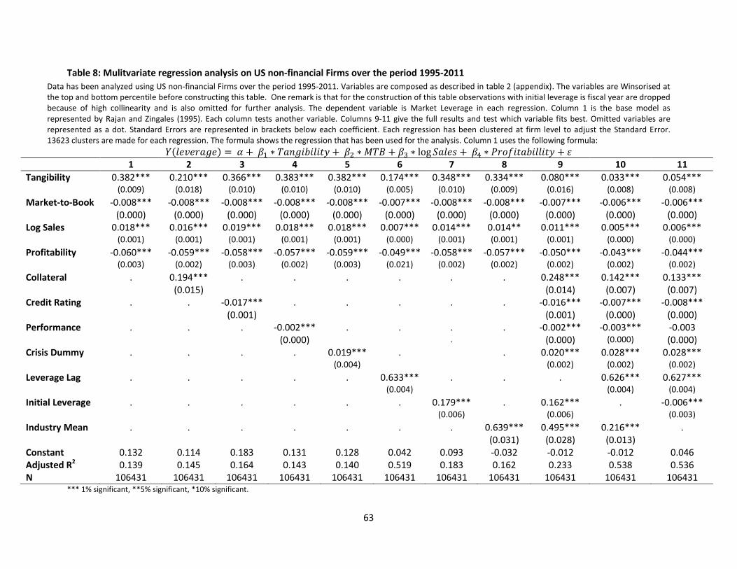
63

Table 8: Mulitvariate regression analysis on US non-financial Firms over the period 1995-2011

Data has been analyzed using US non-financial Firms over the period 1995-2011. Variables are composed as described in table 2 (appendix). The variables are Winsorised at the top and bottom percentile before constructing this table. One remark is that for the construction of this table observations with initial leverage is fiscal year are dropped because of high collinearity and is also omitted for further analysis. The dependent variable is Market Leverage in each regression. Column 1 is the base model as represented by Rajan and Zingales (1995). Each column tests another variable. Columns 9-11 give the full results and test which variable fits best. Omitted variables are represented as a dot. Standard Errors are represented in brackets below each coefficient. Each regression has been clustered at firm level to adjust the Standard Error. 13623 clusters are made for each regression. The formula shows the regression that has been used for the analysis. Column 1 uses the following formula:

1 2 3 4 5 6 7 8 9 10 11

Tangibility 0.382*** 0.210*** 0.366*** 0.383*** 0.382*** 0.174*** 0.348*** 0.334*** 0.080*** 0.033*** 0.054*** (0.009) (0.018) (0.010) (0.010) (0.010) (0.005) (0.010) (0.009) (0.016) (0.008) (0.008)

Market-to-Book -0.008*** -0.008*** -0.008*** -0.008*** -0.008*** -0.007*** -0.008*** -0.008*** -0.007*** -0.006*** -0.006*** (0.000) (0.000) (0.000) (0.000) (0.000) (0.000) (0.000) (0.000) (0.000) (0.000) (0.000) Log Sales 0.018*** 0.016*** 0.019*** 0.018*** 0.018*** 0.007*** 0.014*** 0.014** 0.011*** 0.005*** 0.006*** (0.001) (0.001) (0.001) (0.001) (0.001) (0.000) (0.001) (0.001) (0.001) (0.000) (0.000)

Profitability -0.060*** -0.059*** -0.058*** -0.057*** -0.059*** -0.049*** -0.058*** -0.057*** -0.050*** -0.043*** -0.044*** (0.003) (0.002) (0.003) (0.002) (0.003) (0.021) (0.002) (0.002) (0.002) (0.002) (0.002)

Collateral . 0.194*** . . . . . . 0.248*** 0.142*** 0.133*** (0.015) (0.014) (0.007) (0.007) Credit Rating . . -0.017*** . . . . . -0.016*** -0.007*** -0.008*** (0.001) (0.001) (0.000) (0.000) Performance . . . -0.002*** . . . . -0.002*** -0.003*** -0.003 (0.000) . (0.000) (0.000) (0.000) Crisis Dummy . . . . 0.019*** . . 0.020*** 0.028*** 0.028*** (0.004) (0.002) (0.002) (0.002)

Leverage Lag . . . . . 0.633*** . . . 0.626*** 0.627*** (0.004) (0.004) (0.004)

Initial Leverage . . . . . . 0.179*** . 0.162*** . -0.006*** (0.006) (0.006) (0.003)

Industry Mean . . . . . . . 0.639*** 0.495*** 0.216*** . (0.031) (0.028) (0.013) Constant 0.132 0.114 0.183 0.131 0.128 0.042 0.093 -0.032 -0.012 -0.012 0.046 Adjusted R2 0.139 0.145 0.164 0.143 0.140 0.519 0.183 0.162 0.233 0.538 0.536 N 106431 106431 106431 106431 106431 106431 106431 106431 106431 106431 106431

*** 1% significant, **5% significant, *10% significant.

64

Table 9: Multivariate regression analysis using panel data on US non-financial Firms over the period 1995-2011

Data has been analyzed using US non-financial Firms over the period 1995-2011.Variables are composed as described in table 2 (appendix). The variables are Winsorised at the top and bottom percentile, before constructing this table. One remark is that for the construction of this table observations with initial leverage is fiscal year are dropped because of high collinearity and is also omitted for further analysis. The dependent variable is Market Leverage in columns 1-3. Book Leverage is dependent variable in columns 4-6. Altman’s Z-score is used as dependent variable in columns 7-9. Column 1 is the base model as represented by Rajan and Zingales (1995). Then fixed effects are added to the model. Omitted variables are represented as a dot. Standard Errors are represented in brackets below each coefficient. Each regression has been clustered at firm level to adjust the Standard Error. 13623 clusters are made for each regression. Column 1 is added as comparison. The use of panel data tries to over come the problem that unobservable firm effects are captured in the error term1 of the formula as used in table 8.The formula for firm fixed effects in regression (e.g. column 2) is the following, where N dummies (13624) were created for each firm one.

1 2 3 4 5 6 7 8 9

Tangibility 0.382*** 0.385*** 0.375*** 0.346*** 0.339** 0.341*** -1.542*** -0.340*** -1.807***

(0.010) (0.012) (0.010) (0.012) (0.029) (0.011) (0.037) (0.106) (0.036)

Market-to-Book -0.008*** -0.005*** -0.011*** 0.024*** 0.022*** 0.023*** -0.113*** -0.103*** -0.148***

(0.000) (0.000) (0.000) (0.001) (0.001) (0.001) (0.009) (0.008) (0.009)

Log Sales 0.018*** 0.029*** 0.019*** 0.012*** 0.023** 0.014*** 0.065*** 0.164*** 0.002

(0.001) (0.001) (0.001) (0.001) (0.002) (0.001) (0.005) (0.009) (0.005)

Profitability -0.060*** -0.043*** -0.076*** -0.205*** -0.196*** -0.200*** 4.251*** 4.222*** 4.634***

(0.003) (0.002) (0.003) (0.009) (0.009) (0.009) (0.048) (0.050) (0.051)

Constant 0.133 0.075 0.128 0.072 0.034 0.056 1.399 0.598 2.102

Firm fixed effect No Yes No No Yes No No Yes No

Year fixed effect No No Yes No No Yes No No Yes

Adjusted R2 0.139 0.132 0.154 0.349 0.345 0.315 0.897 0.890 0.888

N 106431 106431 106431 106431 106431 106431 106431 106431 106431

Groups . 13624 16 . 13624 16 . 13624 16

*** 1% significant, **5% significant, *10% significant. 1 , where εit is the error term from the equation in table 8, αi is the unobservable firm effect and uit is the error term that remains after using firm

fixed effects.

Table 10: Regression with crisis years as interaction terms on US non-financial firms over the period 1995-2011

Data has been analyzed using non-financial US Firms over the period 1995-2011. Variables are composed as described in table 2 (appendix). The variables are Winsorised at the top and bottom percentile, before constructing this table. One remark is that for the construction of this table observations with initial leverage is fiscal year are dropped because of high collinearity and is also omitted for further analysis. The dependent variable is Market Leverage. The models are based on the model as represented by Rajan and Zingales (1995). As interaction dummy the crisis years 2001, 2002, 2007 and 2008 are used to spot the differences during crisis years. Omitted variables are represented as a dot. Standard Errors are represented in brackets below each coefficient. Each regression has been clustered at firm level to adjust the Standard Error. 13623 clusters are made for each regression. Column 1 uses the following formula:

1 2 3 4 5 6 7

Crisis dummy 0.007*** 0.017*** -0.012** 0.021*** 0.032*** 0.004* -0.015** (0.003) (0.002) (0.004) (0.002) (0.002) (0.002) (0.007) Tangibility 0.371*** 0.382*** 0.382*** 0.382*** 0.348*** 0.173*** 0.334*** (0.010) (0.010) (0.010) (0.010) (0.010) (0.005) (0.010) Crisis dummy * tangibility 0.044*** . . . . . . (0.007) Market-to-Book -0.008*** -0.008*** -0.008*** -0.008*** -0.008*** -0.007*** -0.008*** (0.000) (0.000) (0.000) (0.000) (0.000) (0.000) (0.000) Crisis dummy * Market-to-Book . -0.001** . . . . . (0.000) Log Sales 0.018*** 0.018*** 0.016*** 0.018*** 0.014*** 0.007*** 0.0069*** (0.001) (0.001) (0.001) (0.001) (0.001) (0.000) (0.001) Crisis dummy * Log Sales . . 0.007*** . . . . (0.001) Profitability -0.059*** -0.059*** -0.060*** -0.063*** -0.057*** -0.048*** -0.056*** (0.003) (0.003) (0.003) (0.003) (0.002) (0.002) (0.002) Crisis dummy * Profitability . . . 0.011*** . . . (0.002) Initial leverage . . . . 0.189*** . . (0.006) Crisis dummy * Initial Leverage . . . . -0.037*** . . (0.005) Market Leverage Lag . . . . . 0.609*** . (0.004) Crisis dummy * Market Leverage Lag . . . . . 0.106*** . (0.006)

66

Industry mean . . . . . . 0.610***

(0.030)

Crisis dummy * Industry mean . . . . . . 0.115***

(0.021)

Constant 0.131 0.127 0.136 0.127 0.085 0.042 -0.027

Adjusted R2

0.140 0.140 0.140 0.140 0.184 0.523 0.163

N 106431 106431 106431 106431 106431 106431 106431

*** 1% significant, **5% significant, *10% significant.

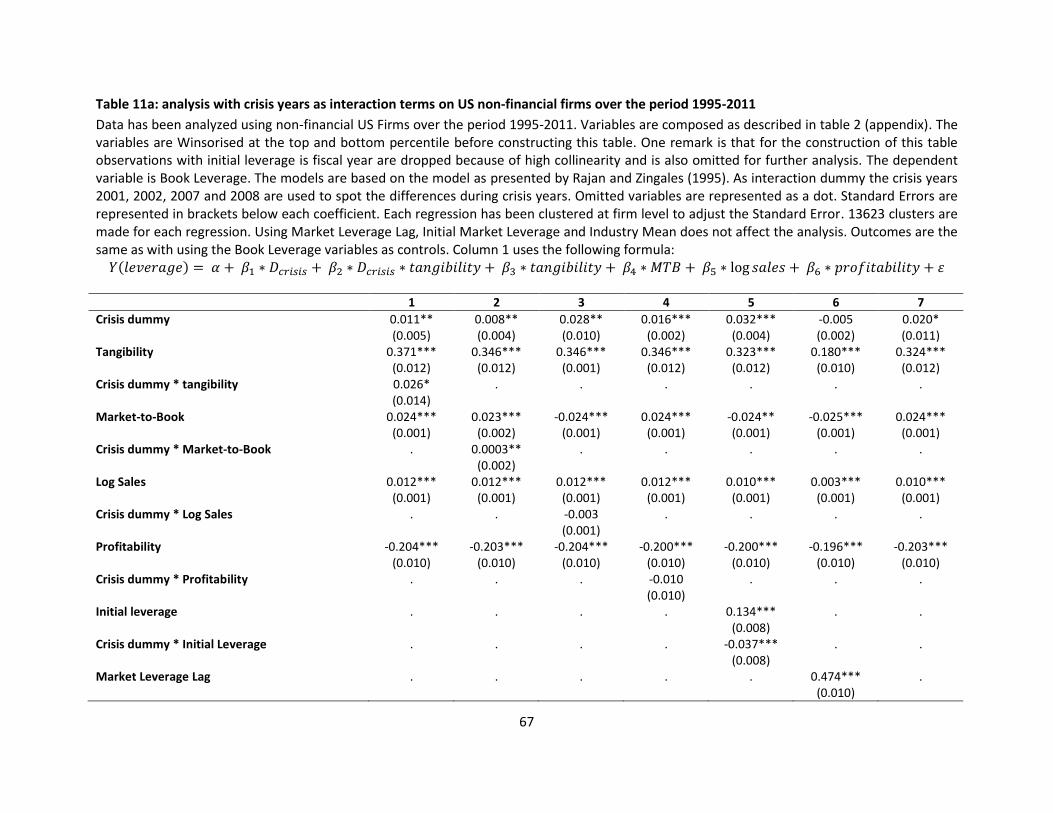
67

Table 11a: analysis with crisis years as interaction terms on US non-financial firms over the period 1995-2011

Data has been analyzed using non-financial US Firms over the period 1995-2011. Variables are composed as described in table 2 (appendix). The variables are Winsorised at the top and bottom percentile before constructing this table. One remark is that for the construction of this table observations with initial leverage is fiscal year are dropped because of high collinearity and is also omitted for further analysis. The dependent variable is Book Leverage. The models are based on the model as presented by Rajan and Zingales (1995). As interaction dummy the crisis years 2001, 2002, 2007 and 2008 are used to spot the differences during crisis years. Omitted variables are represented as a dot. Standard Errors are represented in brackets below each coefficient. Each regression has been clustered at firm level to adjust the Standard Error. 13623 clusters are made for each regression. Using Market Leverage Lag, Initial Market Leverage and Industry Mean does not affect the analysis. Outcomes are the same as with using the Book Leverage variables as controls. Column 1 uses the following formula:

1 2 3 4 5 6 7

Crisis dummy 0.011** 0.008** 0.028** 0.016*** 0.032*** -0.005 0.020* (0.005) (0.004) (0.010) (0.002) (0.004) (0.002) (0.011) Tangibility 0.371*** 0.346*** 0.346*** 0.346*** 0.323*** 0.180*** 0.324*** (0.012) (0.012) (0.001) (0.012) (0.012) (0.010) (0.012) Crisis dummy * tangibility 0.026* . . . . . . (0.014) Market-to-Book 0.024*** 0.023*** -0.024*** 0.024*** -0.024** -0.025*** 0.024*** (0.001) (0.002) (0.001) (0.001) (0.001) (0.001) (0.001) Crisis dummy * Market-to-Book . 0.0003** . . . . . (0.002) Log Sales 0.012*** 0.012*** 0.012*** 0.012*** 0.010*** 0.003*** 0.010*** (0.001) (0.001) (0.001) (0.001) (0.001) (0.001) (0.001) Crisis dummy * Log Sales . . -0.003 . . . . (0.001) Profitability -0.204*** -0.203*** -0.204*** -0.200*** -0.200*** -0.196*** -0.203*** (0.010) (0.010) (0.010) (0.010) (0.010) (0.010) (0.010) Crisis dummy * Profitability . . . -0.010 . . . (0.010) Initial leverage . . . . 0.134*** . . (0.008) Crisis dummy * Initial Leverage . . . . -0.037*** . . (0.008) Market Leverage Lag . . . . . 0.474*** . (0.010)

68

Crisis dummy * Market Leverage Lag . . . . . 0.125*** . (0.012) Industry mean . . . . . . 0.305***

(0.034)

Crisis dummy * Industry mean . . . . . . -0.004

(0.033)

Constant 0069 0.070 0.064 0.067 0.036 0.002 -0.012

Adjusted R2

0.349 0.349 0.349 0.349 0.356 0.425 0.350

N 106431 106431 106431 106431 106431 106431 106431

*** 1% significant, **5% significant, *10% significant.

69

Table 11b: Altman’s Z-score analysis with crisis years as interaction terms on US non-financial firms over the period 1995-2011

Data has been analyzed using non-financial US Firms over the period 1995-2011. Variables are composed as described in table 2 (appendix). The variables are Winsorised at the top and bottom percentile before constructing this table. One remark is that for the construction of this table observations with initial leverage is fiscal year are dropped because of high collinearity and is also omitted for further analysis. The dependent variable is Altman’s Z-score. The models are based on the model as represented by Rajan and Zingales (1995). As interaction dummy the crisis years 2001, 2002, 2007 and 2008 are used to spot the differences during crisis years. Omitted variables are represented as a dot. Standard Errors are represented in brackets below each coefficient. Each regression has been clustered at firm level to adjust the Standard Error. 13623 clusters are made for each regression. Using Market Leverage Lag, Initial Market Leverage and Industry Mean does not affect the analysis. Outcomes are the same as with using the Z-score variables as controls. Column 1 uses the following formula:

1 2 3 4 5 6 7

Crisis dummy -0.161*** -0.068*** -0.192*** -0.111*** -0.137*** -0.122*** -0.171*** (0.021) (0.015) (0.038) (0.010) (0.017) (0.015) (0.038) Tangibility -1.577*** -1.541*** -1.544*** -1.544*** -1.525*** -1.383*** -1.486*** (0.038) (0.037) (0.037) (0.037) (0.037) (0.034) (0.039) Crisis dummy * tangibility 0.122*** . . . . . . (0.048) Market-to-Book -0.114*** -0.109*** -0.114*** -0.114*** -0.114*** -0.115*** -0.114*** (0.009) (0.009) (0.009) (0.009) (0.009) (0.009) (0.009) Crisis dummy * Market-to-Book . -0.020** . . . . . (0.007) Log Sales 0.066*** 0.066*** 0.062*** 0.066*** 0.067*** 0.074*** 0.070*** (0.005) (0.005) (0.005) (0.005) (0.005) (0.005) (0.005) Crisis dummy * Log Sales . . 0.014*** . . . . (0.006) Profitability 4.229*** 4.237*** 4.243*** 4.214*** 4.244*** 4.237*** 4.241*** (0.049) (0.049) (0.049) (0.052) (0.049) (0.049) (0.049) Crisis dummy * Profitability . . . 0.085*** . . . (0.030) Initial leverage . . . . -0.111*** . . (0.025) Crisis dummy * Initial Leverage . . . . 0.026 . . (0.025) Market Leverage Lag . . . . . -0.478*** . (0.034)

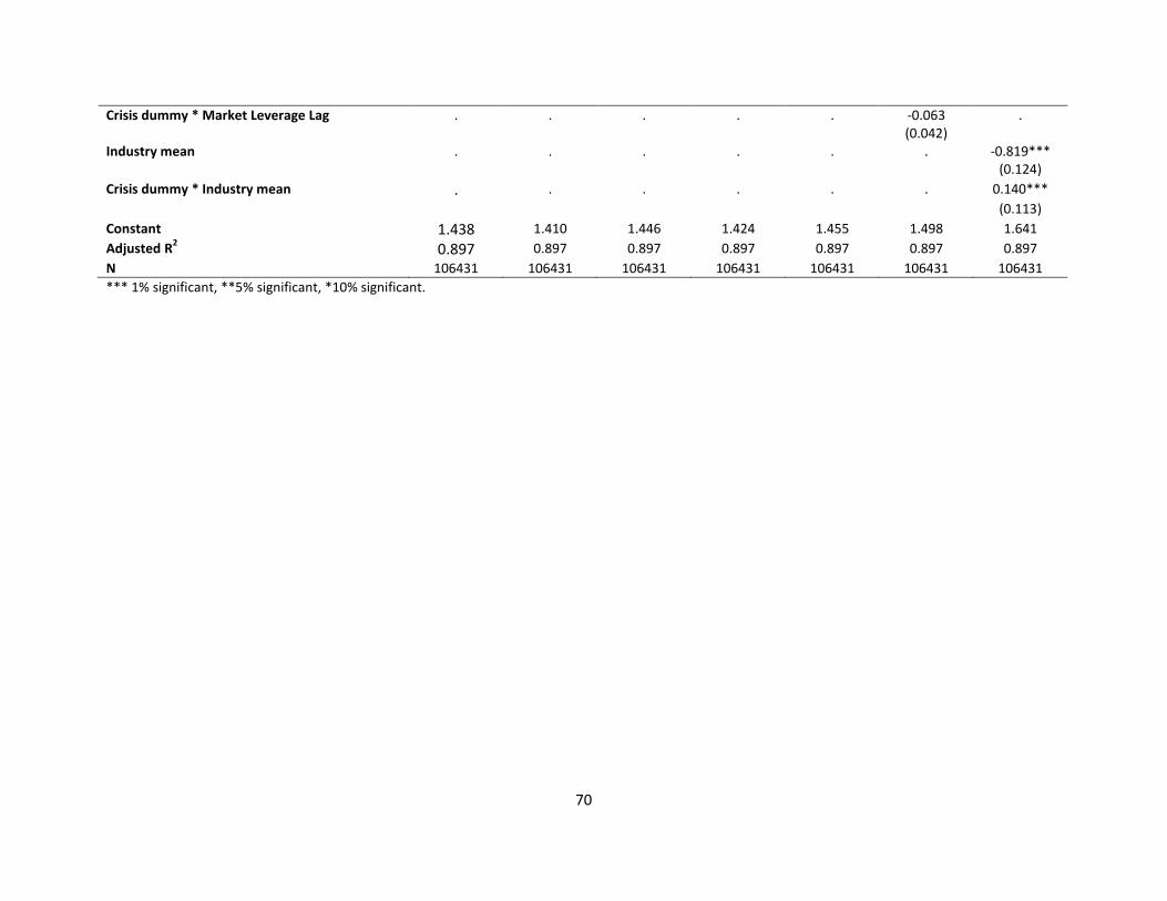
70

Crisis dummy * Market Leverage Lag . . . . . -0.063 . (0.042) Industry mean . . . . . . -0.819***

(0.124)

Crisis dummy * Industry mean . . . . . . 0.140***

(0.113)

Constant 1.438 1.410 1.446 1.424 1.455 1.498 1.641

Adjusted R2

0.897 0.897 0.897 0.897 0.897 0.897 0.897

N 106431 106431 106431 106431 106431 106431 106431

*** 1% significant, **5% significant, *10% significant.

71

Table 12: Regression analysis with Financials as interaction dummy on US firms over the period 1995-2011

Data has been analyzed using all US Firms over the period 1995-2011. Financial firms are defined as SIC codes between 6000 and 6800 (table 3 appendix). Variables are composed as described in table 2 (appendix). The variables are Winsorised at the top and bottom percentile before constructing this table. One remark is that for the construction of this table observations with initial leverage is fiscal year are dropped because of high collinearity and is also omitted for further analysis. The dependent variable is Market Leverage. The models are based on the model as represented by Rajan and Zingales (1995). As interaction dummy financial firms (code 8) are used to spot the differences among financials and non-financials. Omitted variables are represented as a dot. Standard Errors are represented in brackets below each coefficient. Each regression has been clustered at firm level to adjust the Standard Error. 18650 clusters are made for each regression. A (-) means the variable is omitted because of collinearity and in this case financial dummy times industry mean for financials is omitted (Column 7). Column 1 uses the following formula:

1 2 3 4 5 6 7

Financials Dummy 0.120*** 0.111*** -0.031*** 0.120*** 0.024*** -0.004** 0.0115*** (0.050) (0.005) (0.006) (0.005) (0.005) (0.002) (0.005)

Tangibility 0.343*** 0.342*** 0.377*** 0.344*** 0.321*** 0.165*** 0.302*** (0.010) (0.010) (0.010) (0.010) (0.009) (0.004) (0.010)

Financials dummy * Tangibility 0.002 . . . . . . (0.039)

Market-to-Book -0.010*** -0.011*** -0.010*** -0.010*** -0.010*** -0.008*** -0.010*** (0.000) (0.000) (0.000) (0.000) (0.000) (0.000) (0.000) Financials dummy * Market-to-Book . 0.006*** . . . . . (0.001) Log Sales 0.032*** 0.032*** 0.019*** 0.032*** 0.021*** 0.010*** 0.030*** (0.001) (0.001) (0.001) (0.001) (0.001) (0.000) (0.001)

Financials dummy * Log Sales . . 0.044*** . . . . (0.002)

Profitability -0.090*** -0.092*** -0.076*** -0.091*** -0.077*** -0.060*** -0.088*** (0.003) (0.003) (0.003) (0.003) (0.003) (0.002) (0.003) Financials dummy * Profitability . . . -0.022*** . . . (0.003)

Initial Market Leverage . . . . 0.175*** . . (0.006)

Financials dummy * Initial Market Leverage . . . . 0.311*** . . (0.013)

72

Leverage lag . . . . . 0.631*** . (0.004) Financials dummy * leverage lag . . . . . 0.182*** . (0.006)

Industry mean . . . . . . 0.553*** (0.031) Financials dummy * Industry mean . . . . . . - - Constant 0.077 0.081 0.132 0.077 0.073 0.036 -0.069 Adjusted R2 0.158 0.159 0.185 0.159 0.253 0.581 0.172 N 142391 142391 142391 142391 142391 142391 142391

*** Significant at 1%, ** significant at 5%, * significant at 10%.

73

Table 13a: Book Leverage analysis with Financials as interaction terms on US firms over the period 1995-2011.

Data has been analyzed using all US Firms over the period 1995-2011. Financial firms are defined as SIC codes between 6000 and 6800 (table 3 appendix). Variables are composed as described in table 2 (appendix). The variables are Winsorised at the top and bottom percentile, before constructing this table. One remark is that for the construction of this table observations with initial leverage is fiscal year are dropped because of high collinearity and is also omitted for further analysis. The dependent variable is Book Leverage. The models are based on the model as represented by Rajan and Zingales (1995). As interaction dummy financial firms (code 8) are used to spot the differences among financials and non-financials. Omitted variables are represented as a dot. Standard Errors are represented in brackets below each coefficient. Each regression has been clustered at firm level to adjust the Standard Error. 13623 clusters are made for each regression. A (-) means the variable is omitted because of collinearity and in this case financial dummy times industry mean for financials is omitted (Column 7). Using Market Leverage Lag, Initial Market Leverage and Industry Mean does not affect the analysis. Outcomes are the same as with using the Book Leverage variables as controls. Column 1 uses the following formula:

1 2 3 4 5 6 7

Financials Dummy 0.026*** -0.038*** -0.018* 0.034*** -0.023*** -0.014*** 0.032*** (0.006) (0.007) (0.010) (0.006) (0.006) (0.005) (0.006) Tangibility 0.329*** 0.340*** 0.351*** 0.340*** 0.324*** 0.201*** 0.320*** (0.010) (0.010) (0.010) (0.010) (0.010) (0.010) (0.011) Financials dummy * Tangibility 0.157*** . . . . . . (0.050)

Market-to-Book 0.022*** 0.023*** 0.022*** 0.022*** 0.022*** 0.024*** 0.022*** (0.001) (0.001) (0.001) (0.001) (0.001) (0.001) (0.001) Financials dummy * Market-to-Book . -0.003 . . . . . (0.005) Log Sales 0.018*** 0.018*** 0.013*** 0.018*** 0.011*** 0.004*** 0.017*** (0.001) (0.001) (0.001) (0.001) (0.001) (0.001) (0.001)

Financials dummy * Log Sales . . 0.015*** . . . . (0.002)

Profitability -0.210*** -0.209*** -0.206*** -0.211*** -0.203*** -0.192*** -0.209*** (0.009) (0.009) (0.009) (0.009) (0.009) (0.008) (0.009)

Financials dummy * Profitability . . . 0.010 . . . (0.035)

Initial Market Leverage . . . . 0.118*** . . (0.007)

74

Financials dummy * Initial Market Leverage . . . . 0.184*** . . (0.016)

Leverage lag . . . . . 0.475*** . (0.008) Financials dummy * leverage lag . . . . . 0.007 . (0.016)

Industry mean . . . . . . 0.258*** (0.031) Financials dummy * Industry mean . . . . . . - - Constant 0.048 0.044 0.065 0.046 0.004 0.004 -0.022 Adjusted R2 0.318 0.318 0.319 0.317 0.337 0.420 0.319 N 142391 142391 142391 142391 142391 142391 142391

*** Significant at 1%, ** significant at 5%, * significant at 10%.

75

Table 13b: Altman’s Z-score analysis with Financials as interaction terms on US firms over the period 1995-2011.

Data has been analyzed using all US Firms over the period 1995-2011. Financial firms are defined as SIC codes between 6000 and 6800 (table 3 appendix). Variables are composed as described in table 2 (appendix). The variables are Winsorised at the top and bottom percentile before constructing this table. One remark is that for the construction of this table observations with initial leverage is fiscal year are dropped because of high collinearity and is also omitted for further analysis. The dependent variable is Altman’s Z-score. The models are based on the model as represented by Rajan and Zingales (1995). As interaction dummy financial firms (code 8) are used to spot the differences among financials and non-financials. Omitted variables are represented as a dot. Standard Errors are represented in brackets below each coefficient. Each regression has been clustered at firm level to adjust the Standard Error. 13623 clusters are made for each regression. A (-) means the variable is omitted because of collinearity and in this case financial dummy times industry mean for financials is omitted (Column 7). Using Market Leverage Lag, Initial Market Leverage and Industry Mean does not affect the analysis. Outcomes are the same as with using the Z-score variables as controls. Column 1 uses the following formula:

1 2 3 4 5 6 7

Financials Dummy -1.276*** -1.326*** -1.078*** -1.175*** -1.171*** -1.166*** -1.166*** (0.019) (0.021) (0.029) (0.019) (0.024) (0.025) (0.019) Tangibility -1.492*** -1.374*** -1.370*** -1.353*** -1.334*** -1.219*** -1.1292** (0.032) (0.032) (0.033) (0.032) (0.033) (0.034) (0.034) Financials dummy * Tangibility 2.1958*** . . . . . . (0.113)

Market-to-Book -0.084*** -0.097*** -0.082*** -0.083*** -0.083*** -0.084*** -0.083*** (0.008) (0.007) (0.008) (0.008) (0.008) (0.008) (0.008) Financials dummy * Market-to-Book . 0.104*** . . . . . (0.015) Log Sales 0.061*** 0.056*** 0.068*** 0.060*** 0.063*** 0.071*** 0.063*** (0.004) (0.003) (0.005) (0.004) (0.004) (0.004) (0.004)

Financials dummy * Log Sales . . -0.028*** . . . . (0.005)

Profitability 4.286*** 4.248*** 4.280*** 4.297*** 4.286*** 4.274*** 4.285*** (0.043) (0.040) (0.044) (0.043) (0.043) (0.043) (0.043)

Financials dummy * Profitability . . . -0.142*** . . . (0.043)

Initial Market Leverage . . . . -0.089*** . . (0.023)

76

Financials dummy * Initial Market Leverage . . . . 0.001 . . (0.044)

Leverage lag . . . . . -0.433*** . (0.030) Financials dummy * leverage lag . . . . . 0.124*** . (0.043)

Industry mean . . . . . . -0.764*** (0.112) Financials dummy * Industry mean . . . . . . - - Constant 1.332 1.358 1.263 1.300 1.312 1.345 1.499 Adjusted R2 0.885 0.886 0.884 0.884 0.884 0.885 0.884 N 142391 142391 142391 142391 142391 142391 142391

*** Significant at 1%, ** significant at 5%, * significant at 10%.

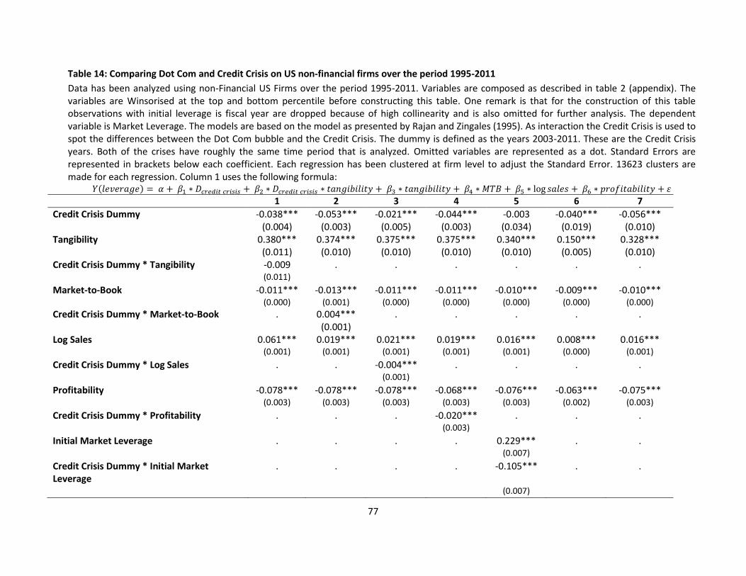
77

Table 14: Comparing Dot Com and Credit Crisis on US non-financial firms over the period 1995-2011

Data has been analyzed using non-Financial US Firms over the period 1995-2011. Variables are composed as described in table 2 (appendix). The variables are Winsorised at the top and bottom percentile before constructing this table. One remark is that for the construction of this table observations with initial leverage is fiscal year are dropped because of high collinearity and is also omitted for further analysis. The dependent variable is Market Leverage. The models are based on the model as presented by Rajan and Zingales (1995). As interaction the Credit Crisis is used to spot the differences between the Dot Com bubble and the Credit Crisis. The dummy is defined as the years 2003-2011. These are the Credit Crisis years. Both of the crises have roughly the same time period that is analyzed. Omitted variables are represented as a dot. Standard Errors are represented in brackets below each coefficient. Each regression has been clustered at firm level to adjust the Standard Error. 13623 clusters are made for each regression. Column 1 uses the following formula:

1 2 3 4 5 6 7

Credit Crisis Dummy -0.038*** -0.053*** -0.021*** -0.044*** -0.003 -0.040*** -0.056*** (0.004) (0.003) (0.005) (0.003) (0.034) (0.019) (0.010) Tangibility 0.380*** 0.374*** 0.375*** 0.375*** 0.340*** 0.150*** 0.328*** (0.011) (0.010) (0.010) (0.010) (0.010) (0.005) (0.010) Credit Crisis Dummy * Tangibility -0.009 . . . . . . (0.011)

Market-to-Book -0.011*** -0.013*** -0.011*** -0.011*** -0.010*** -0.009*** -0.010*** (0.000) (0.001) (0.000) (0.000) (0.000) (0.000) (0.000) Credit Crisis Dummy * Market-to-Book . 0.004*** . . . . . (0.001) Log Sales 0.061*** 0.019*** 0.021*** 0.019*** 0.016*** 0.008*** 0.016*** (0.001) (0.001) (0.001) (0.001) (0.001) (0.000) (0.001)

Credit Crisis Dummy * Log Sales . . -0.004*** . . . . (0.001)

Profitability -0.078*** -0.078*** -0.078*** -0.068*** -0.076*** -0.063*** -0.075*** (0.003) (0.003) (0.003) (0.003) (0.003) (0.002) (0.003)

Credit Crisis Dummy * Profitability . . . -0.020*** . . . (0.003)

Initial Market Leverage . . . . 0.229*** . . (0.007)

Credit Crisis Dummy * Initial Market Leverage

. . . . -0.105*** . .

(0.007)

78

Leverage lag . . . . . 0.595*** . (0.005) Credit Crisis Dummy * leverage lag . . . . . 0.080*** . (0.006)

Industry mean . . . . . . 0.605*** (0.033) Credit Crisis Dummy * Industry mean . . . . . . 0.054*** (0.033) Constant 0.149 0.157 0.142 0.152 0.092 0.062 -0.004 Adjusted R2 0.147 0.149 0.148 0.148 0.195 0.524 0.168 N 106417 106417 106417 106417 106417 106417 106417

*** Significant at 1%, ** significant at 5%, * significant at 10%.

79

Table 15a: Comparing Dot Com and Credit Crisis on Book Leverage using US non-financial firms over the period 1995-2011

Data has been analyzed using non-Financial US Firms over the period 1995-2011. Variables are composed as described in table 2 (appendix). The variables are Winsorised at the top and bottom percentile before constructing this table. One remark is that for the construction of this table observations with initial leverage is fiscal year are dropped because of high collinearity and is also omitted for further analysis. The dependent variable is Book Leverage. The models are based on the model as presented by Rajan and Zingales (1995). As interaction the Credit Crisis is used to spot the differences between the Dot Com bubble and the Credit Crisis. The dummy is defined as the years 2003-2011. These are the Credit Crisis years. Both of the crises have roughly the same time period that is analyzed. Omitted variables are represented as a dot. Standard Errors are represented in brackets below each coefficient. Each regression has been clustered at firm level to adjust the Standard Error. 13623 clusters are made for each regression. Using Market Leverage Lag, Initial Market Leverage and Industry Mean does not affect the analysis. Outcomes are the same as with using the Book Leverage variables as controls. Column 1 uses the following formula:

1 2 3 4 5 6 7

Credit Crisis Dummy 0.014*** 0.040*** 0.046*** -0.016*** 0.013*** -0.021*** 0.011 (0.006) (0.005) (0.012) (0.004) (0.004) (0.004) (0.014) Tangibility 0.379*** 0.339*** 0.340*** 0.341*** 0.318*** 0.185*** 0.319*** (0.012) (0.011) (0.011) (0.011) (0.011) (0.010) (0.011) Credit Crisis Dummy * Tangibility -0.080 . . . . . . (0.015)

Market-to-Book 0.023*** 0.017*** 0.023*** 0.022*** 0.023*** 0.025*** 0.023*** (0.001) (0.002) (0.001) (0.001) (0.001) (0.001) (0.001) Credit Crisis Dummy * Market-to-Book . 0.011*** . . . . . (0.011) Log Sales 0.014*** 0.014*** 0.020*** 0.014*** 0.012*** 0.005*** 0.012*** (0.001) (0.001) (0.001) (0.001) (0.001) (0.001) (0.001)

Credit Crisis Dummy * Log Sales . . -0.012*** . . . . (0.002)

Profitability -0.202*** -0.197*** -0.202*** -0.168*** -0.200*** -0.190*** -0.200*** (0.008) (0.008) (0.008) (0.010) (0.008) (0.008) (0.008)

Credit Crisis Dummy * Profitability . . . -0.064*** . . . (0.013)

Initial Market Leverage . . . . 0.146*** . . (0.008)

80

Credit Crisis Dummy * Initial Market Leverage . . . . -0.056*** . . (0.011)

Leverage lag . . . . . 0.430*** . (0.009) Credit Crisis Dummy * leverage lag . . . . . 0.108*** . (0.012)

Industry mean . . . . . . 0.324*** (0.033) Credit Crisis Dummy * Industry mean . . . . . . -0.060*** (0.041) Constant 0.057 0.085 0.043 0.074 0.032 0.008 -0.016 Adjusted R2 0.315 0.319 0.316 0.317 0.323 0.408 0.317 N 106417 106417 106417 106417 106417 106417 106417

*** Significant at 1%, ** significant at 5%, * significant at 10%.

81

Table 15b: Comparing Dot Com and Credit Crisis on Altman’s Z-score using US non-financial firms over the period 1995-2011

Data has been analyzed using non-Financial US Firms over the period 1995-2011. Variables are composed as described in table 2 (appendix). The variables are Winsorised at the top and bottom percentile, before constructing this table. One remark is that for the construction of this table observations with initial leverage is fiscal year are dropped because of high collinearity and is also omitted for further analysis. The dependent variable is Altman’s Z-score. The models are based on the model as represented by Rajan and Zingales (1995). As interaction the Credit Crisis is used to spot the differences between the Dot Com bubble and the Credit Crisis. The dummy is defined as the years 2003-2011. These are the Credit Crisis years. Both of the crises have roughly the same time period that is analyzed. Omitted variables are represented as a dot. Standard Errors are represented in brackets below each coefficient. Each regression has been clustered at firm level to adjust the Standard Error. 13623 clusters are made for each regression. Using Market Leverage Lag, Initial Market Leverage and Industry Mean does not affect the analysis. Outcomes are the same as with using the Z-score variables as controls. Column 1 uses the following formula:

1 2 3 4 5 6 7

Credit Crisis Dummy -0.190*** -0.086*** -0.112*** -0.134*** -0.137*** -0.072*** -0.189*** (0.022) (0.019) (0.042) (0.012) (0.018) (0.016) (0.045) Tangibility -1.632*** -1.549*** -1.553*** -1.552*** -1.535*** -1.403*** -1.496** (0.040) (0.033) (0.033) (0.032) (0.033) (0.034) (0.035) Credit Crisis Dummy * Tangibility 0.169*** . . . . . . (0.048)

Market-to-Book -0.101*** -0.090*** -0.101*** -0.100*** -0.102*** -0.103*** -0.102*** (0.008) (0.010) (0.007) (0.008) (0.008) (0.008) (0.008) Credit Crisis Dummy * Market-to-Book . -0.020*** . . . . . (0.001) Log Sales 0.076*** 0.076*** 0.079*** 0.076*** 0.077*** 0.084*** 0.079*** (0.005) (0.005) (0.006) (0.005) (0.005) (0.005) (0.005)

Credit Crisis Dummy * Log Sales . . -0.007 . . . . (0.007)

Profitability 4.179*** 4.170*** 4.179*** 4.136*** 4.178*** 4.167*** 4.174*** (0.043) (0.043) (0.043) (0.043) (0.043) (0.043) (0.043)

Credit Crisis Dummy * Profitability . . . 0.082** . . . (0.021)

Initial Market Leverage . . . . -0.081*** . . (0.027)

82

Credit Crisis Dummy * Initial Market Leverage . . . . -0.024 . . (0.031)

Leverage lag . . . . . -0.308*** . (0.030) Credit Crisis Dummy * leverage lag . . . . . -0.305*** . (0.040)

Industry mean . . . . . . -0.929*** (0.115) Credit Crisis Dummy * Industry mean . . . . . . 0.144 (0.137) Constant 1.411 1.357 1.373 1.380 1.405 1.413 1.605 Adjusted R2 0.890 0.890 0.890 0.890 0.890 0.891 0.890 N 142391 142391 142391 142391 142391 142391 142391

*** Significant at 1%, ** significant at 5%, * significant at 10%.

83

Table 16: Descriptive statistic comparison between Dot Com bubble and Credit Crisis

This table has been constructed using non-financial US firms over the period 1995-2011. Variables are composed as described in table 2 (appendix). The variables are Winsorised at the top and bottom percentile, before constructing this table. Another remark is that for the construction of this table observations with initial leverage is fiscal year are dropped because of high collinearity and is also omitted for further analysis. A dummy was made to divide the data between the Dot Com bubble and the Credit Crisis. The dummy is defined as the years 2003-2011 so the Credit Crisis years. Both of the crises have roughly the same time period that is analyzed. The column ‘Change’ shows the change in mean between the Dot Com bubble and the Credit Crisis. A (-) represents a lower mean, (+) represents higher and (~) represent ‘little’ change and (=) is in the situation it remains the same.

Dot Com bubble Mean

Standard deviation

Change Credit Crisis Mean

Standard deviation

Market Leverage 0.291 0.334 + 0.316 0.343 Book Leverage 0.305 0.493 + 0.339 0.568 Tangibility 0.268 0.250 ~ 0.265 0.253 Market-to-Book 2.966 6.097 ~ 2.938 6.658 Log Sales 4.446 2.891 ~ 4.533 3.033 Profitability -0.122 0.823 - -0.211 1.006 Collateral 0.375 0.269 ~ 0.363 0.272 Altman’s Z-score 0.462 4.218 -- -0.019 5.107 Current ratio 2.560 3.208 - 2.502 3.268 Alternative Leverage 9.230 105.646 -- 3.093 103.864 Performance 0.635 8.892 -- -2.373 9.314 Initial Leverage 0.349 0.400 = 0.349 0.401 Note: Some results are hard to interpret since the standard deviations are high compared to the means. Therefore they will not be analyzed.

Table 17: Leverage (mean) comparison between the Dot Com bubble and the Credit Crisis

This table has been constructed using non-financial US firms over the period 1995-2011. Variables are composed as described in table 2 (appendix). The variables are Winsorised at the top and bottom percentile, before constructing this table. This table shows the mean for the different leverage measures and their standard deviations in brackets below. The chosen years are around the Dot Com Bubble and the Credit Crisis.

2000 2001 2002 2007 2008 2009

Market Leverage Mean 0.336 0.324 0.338 0.248 0.350 0.295 (0.340) (0.348) (0.353) (0.306) (0.348) (0.330)

Book Leverage mean 0.317 0.348 0.347 0.312 0.345 0.336 (0.475) (0.549) (0.578) (0.556) (0.590) (0.595)

Altman’s Z-score Mean 0.247 -0.142 -0.093 0.172 0.039 0.413 (4.381) (5.085) (5.266) (4.788) (5.247) (4.571)

Alternative leverage mean -4.118 -4.726 -0.520 9.965 13.863 22.439 (99.729) (96.257) (95.341) (114.6424) (110.931) (127.601)

84

Graph 1: Changes in Market Leverage over time

This graph has been constructed using all US firms over the period 1996-2010. Financial firms are defined as SIC codes between 6000 and 6800 (table 3 appendix). Variables are composed as described in table 2 (appendix). The variables are Winsorised at the top and bottom percentile, before constructing this graph. Another remark is that for the construction of this graph observations with initial leverage is fiscal year are dropped because of high collinearity. Therefore 1995 is omitted. 2011 is omitted because of too little observations. The graph shows the changes in Market Leverage for both the financial as the non-financial US firms over time. The graph shows the mean and median for both of them. For the construction of this graph all observations with Market Leverage is 0 and 1 are deleted.

0

0,1

0,2

0,3

0,4

0,5

0,6

0,7

1996 1997 1998 1999 2000 2001 2002 2003 2004 2005 2006 2007 2008 2009 2010

non-financials mean

non-financials median

financials mean

financials median

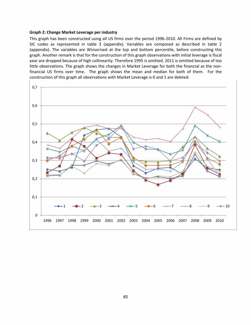
85

Graph 2: Change Market Leverage per industry

This graph has been constructed using all US firms over the period 1996-2010. All Firms are defined by SIC codes as represented in table 3 (appendix). Variables are composed as described in table 2 (appendix). The variables are Winsorised at the top and bottom percentile, before constructing this graph. Another remark is that for the construction of this graph observations with initial leverage is fiscal year are dropped because of high collinearity. Therefore 1995 is omitted. 2011 is omitted because of too little observations. The graph shows the changes in Market Leverage for both the financial as the non-financial US firms over time. The graph shows the mean and median for both of them. For the construction of this graph all observations with Market Leverage is 0 and 1 are deleted.

0

0,1

0,2

0,3

0,4

0,5

0,6

0,7

1996 1997 1998 1999 2000 2001 2002 2003 2004 2005 2006 2007 2008 2009 2010

1 2 3 4 5 6 7 8 9 10

86

Graph 3: Change of Market Leverage over time based on size

This graph has been constructed using non-financial US firms over the period 1996-2010. Variables are composed as described in table 2 (appendix). The variables are Winsorised at the top and bottom percentile, before constructing this table. Another remark is that for the construction of this graph observations with initial leverage is fiscal year are dropped because of high collinearity. Therefore 1995 is omitted. 2011 is omitted because of too little observations. The graph shows the mean of Market Leverage over time per ‘decile’. The deciles are constructed using Log Sales as benchmark for firm size. For the construction of this graph all observations with Market Leverage is 0 and 1 are deleted.

* Although this is used to look at differences in size it can be seen that the mean per size decile converges over

time.

0

0,05

0,1

0,15

0,2

0,25

0,3

0,35

0,4

0,45

1996 1997 1998 1999 2000 2001 2002 2003 2004 2005 2006 2007 2008 2009 2010

1 2 3 4 5 6 7 8 9 10

87

Graph 4: Convergence of Market Leverage based on initial leverage

This graph has been constructed using non-Financial US firms over the period 1996-2010. Variables are composed as described in table 2 (appendix). The variables are Winsorised at the top and bottom percentile, before constructing this table. Another remark is that for the construction of this graph observations with initial leverage is fiscal year are dropped because of high collinearity. Therefore 1995 is omitted. 2011 is omitted because of too little observations. This graph shows the convergence over time based on the initial Market Leverage of each firm per (initial) decile. For the construction of this graph variable initial leverage is represented in ‘deciles’. Furthermore observations with Market Leverage is 0 and 1 are deleted.

0

0,1

0,2

0,3

0,4

0,5

0,6

0,7

1995 1996 1997 1998 1999 2000 2001 2002 2003 2004 2005 2006 2007 2008 2009 2010

88

Graph 5: Change of Book Leverage over time

This graph has been constructed using all US firms over the period 1996-2010. Financial firms are defined as SIC codes between 6000 and 6800 (table 3 appendix). Variables are composed as described in table 2 (appendix). The variables are Winsorised at the top and bottom percentile, before constructing this graph. Another remark is that for the construction of this graph observations with initial leverage is fiscal year are dropped because of high collinearity. Therefore 1995 is omitted. 2011 is omitted because of too little observations. The graph shows the mean and median of Book Leverage over the time period 1996-2010. For the construction of this graph all observations with Market Leverage is 0 and 1 are deleted to compare with the graph 1.

0

0,05

0,1

0,15

0,2

0,25

0,3

0,35

0,4

0,45

1996 1997 1998 1999 2000 2001 2002 2003 2004 2005 2006 2007 2008 2009 2010

book leverage mean book leverage median

89

Graph 6: Change of Altman’s Z-score over time

This graph has been constructed using all US firms over the period 1996-2010. Financial firms are defined as SIC codes between 6000 and 6800 (table 3 appendix). Variables are composed as described in table 2 (appendix). The variables are Winsorised at the top and bottom percentile, before constructing this graph. Another remark is that for the construction of this graph observations with initial leverage is fiscal year are dropped because of high collinearity. Therefore 1995 is omitted. 2011 is omitted because of too little observations. The graph shows the mean and median of Altman’s Z-score over the time period 1996-2010. For the construction of this graph all observations with Market Leverage is 0 and 1 are deleted in order to give the same results and easier comparison with the graph 1.

-0,2

0

0,2

0,4

0,6

0,8

1

1,2

1,4

1,6

1996 1997 1998 1999 2000 2001 2002 2003 2004 2005 2006 2007 2008 2009 2010

Z score mean

Z score median