did the asset price bubble matter for japanese banking ... · munich personal repec archive did the...
TRANSCRIPT
Munich Personal RePEc Archive
Did The Asset Price Bubble Matter For
Japanese Banking Crisis In The 1990s?
Hossain, Monzur
2004
Online at https://mpra.ub.uni-muenchen.de/24738/
MPRA Paper No. 24738, posted 02 Sep 2010 01:03 UTC
1
Session: 5b-3
9th
CONVENTION OF THE EAST ASIAN ECONOMIC ASSOCIATION
13-14 November 2004, Hong Kong
Did The Asset Price Bubble Matter For Japanese Banking Crisis In The 1990s?
MONZUR HOSSAIN+
Affiliations:
(1) National Graduate Institute for Policy Studies, Tokyo
(2) Bangladesh Bank (the central bank of Bangladesh)
Address for correspondence:
2-2 Wakamatsu-cho, Shinjuku-ku
Tokyo 162-8677, Japan
Tel: 81-48-958-9992 (Res.)
81-090-1107-4330 (Cell)
E-mail: [email protected]
URL: www.geocities.com/monzurhossain
Abstract
Regarding the causality of Japanese banking crisis, two views are popular: (i) slow and
undirected financial deregulations in the 1980s caused trouble for the banks in adjusting with the
new environment, and (ii) banks shifted their business in SME market and real estate businesses
aggressively in the era of protracted monetary easing in the mid 1980s, that finally contributed to
banking failures after the curbed down of asset prices. Instead of these two views, this paper
shows that the continuous declining trend of banks profitability (e.g. ROA or ROE) from 1970
was a warning signal for banking crisis, which was just accelerated by the bubble burst. Without
any shock (monetary or bubble phenomenon) during the later half of the 1980s, it would take
some more time to reach the crisis situation. The paper also highlights some potential causes of
declining trend of banks profitability. For analysis, Kaplan-Meire’s Product-Limit method is
applied to estimate the survival functions and cause-specific hazard rates for the Japanese banks,
along with Cox’s Proportional Hazards Model is used to find the significance of regression
coefficients. Again, Accelerated failure time model is used to see whether collapse of the bubble
accelerated the failure of the banks. Moreover, cointegration test and Granger causality test have
been performed to identify the long- term causality of banks’ declining profitability. The issue is
not only important for the Japanese economy, but also instructive for other big Asian economies.
Key words: Japanese banking crisis, Bubble economy, and Survival analysis.
JEL classification: E44, G21, G28, G33, C41.
+ The views expressed in this paper are my own and do not necessarily reflect those of the institutions with which I
am affiliated. Any remaining errors are, of course, mine.
2
1. Introduction
The failure of a large number of Japanese banks during the 1990s following the burst of the
asset price bubble in early 1990 synthesizes a vast literature during last few years focusing the
causes and consequences of the crisis, which is still growing. The growing concern on this issue
indicates that the issue has not yet ended. Since the crisis afflicted the economy, therefore it
becomes a vital policy issue- why has the successful banking system of the 1960s and 1970s
failed? The experience of 1990s suggests that economic, social and political cost of crisis,
whatever it may be policy induced or structural could be formidable.
Two stylized facts have emerged in explaining the crisis- one, the transition from highly
regulated main bank system through slow and undirected financial deregulations caused
problems for the banks to adjust with the new environment; and that’s why their speculative
behavior during the asset price bubble to increase short-term profit made them vulnerable after
burst of the bubble (among others, see Hoshi, 2001; Ueda, 2000; Cargill, 2000). The other
focuses on the monetary policy effectiveness in the 1980s. Their view is that in the era of
protracted monetary easing during the mid 1980s, banks expanded their business aggressively to
the SME market, real estate businesses as they lost their big customers of main bank
arrangements, which created the problem of moral hazard and asymmetry of information. Since
their loan was secured by collateral assets (land), the continuing plunge of land prices made the
loan uncollectible and a huge burden of non-performing loan occurred that ultimately contributed
to banking failures (for example, see Okina, 2001; Aoki et al. 1994, Cargill, 2000). Moreover,
some researches combine ‘the both’ as the causes of the banking crisis.
In contrast, the objective of this paper is to reexamine the causality of banking crisis from
different point of view. It is apparent that banks were becoming weaker during the main bank
regime in terms of their earnings. We may guess that this weak position leads the management to
behave speculative in the era of protracted monetary easing and asset price bubble just to survive.
If they were strong in their financial position, they would not behave speculative, or their
speculative behavior would not make them vulnerable to crisis. Therefore the proposition gives
importance singularly on the management efficiency of the Japanese banking industry.
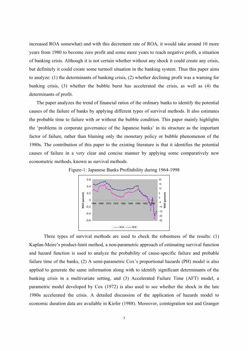
This paper argues that long-term declining profitability since 1970 (Figure 1) was a warning
signal of banking crisis, which was just accelerated by the burst of the bubble. This declining
trend indicates that the bank-management was not so efficient to handle the profitable lending
opportunities in liberalized condition too. Total decrement of ROA per year is estimated around
-0.025 between 1970 and 1980. Without any exogenous shock (monetary shock in the 1980s
3
increased ROA somewhat) and with this decrement rate of ROA, it would take around 10 more
years from 1980 to become zero profit and some more years to reach negative profit, a situation
of banking crisis. Although it is not certain whether without any shock it could create any crisis,
but definitely it could create some turmoil situation in the banking system. Thus this paper aims
to analyze: (1) the determinants of banking crisis, (2) whether declining profit was a warning for
banking crisis, (3) whether the bubble burst has accelerated the crisis, as well as (4) the
determinants of profit.
The paper analyzes the trend of financial ratios of the ordinary banks to identify the potential
causes of the failure of banks by applying different types of survival methods. It also estimates
the probable time to failure with or without the bubble condition. This paper mainly highlights
the ‘problems in corporate governance of the Japanese banks’ in its structure as the important
factor of failure, rather than blaming only the monetary policy or bubble phenomenon of the
1980s. The contribution of this paper to the existing literature is that it identifies the potential
causes of failure in a very clear and concise manner by applying some comparatively new
econometric methods, known as survival methods.
Figure-1: Japanese Banks Profitability during 1964-1998
-0.6
-0.4
-0.2
0
0.2
0.4
0.6
1964 1968 1972 1976 1980 1984 1988 1992 1996
RO
A (
perc
en
t)
-25
-20
-15
-10
-5
0
5
10
15
20
RO
E (
perc
en
t)
ROA ROE
Three types of survival methods are used to check the robustness of the results: (1)
Kaplan-Meire’s product-limit method, a non-parametric approach of estimating survival function
and hazard function is used to analyze the probability of cause-specific failure and probable
failure time of the banks, (2) A semi-parametric Cox’s proportional hazards (PH) model is also
applied to generate the same information along with to identify significant determinants of the
banking crisis in a multivariate setting, and (3) Accelerated Failure Time (AFT) model, a
parametric model developed by Cox (1972) is also used to see whether the shock in the late
1980s accelerated the crisis. A detailed discussion of the application of hazards model to
economic duration data are available in Kiefer (1988). Moreover, cointegration test and Granger
4
causality test have been performed to identify long-term causal relationship of significant
determinants of banks’ failure and low profitability.
The paper proceeds as follows. After the introduction, Section 2 discusses about the
evolution and failure of the Japanese banks. Section 3 highlights potential determinants of
banking failure, Section 4 gives a short description of data, Section 5 describes the empirical
survival methods as well as demonstrates results, Section 6 discusses about potential
determinants of banks profitability and identifies long term determinants of banks profit by
performing time series analysis, and finally Section 7 concludes the paper.
2. Evolution and Failure of Japanese banking system
2.1 Evolution of banking system
The Japanese financial system is predominantly bank-based. Post-war Japanese financial system
was highly regulated and banks were heavily dependent on Bank of Japan’s (BOJ) subsidies
(window guidance) and borrowings of enterprise groups. The characteristics of Japanese model
of financial system during post-war economic growth included high debt/equity ratios, greater
reliance on bank loans than securities markets, closer relationship between banks and borrowers,
extensive corporate cross-shareholding, greater guidance from the government in credit
allocation etc. The system is well known as ‘main bank’ system. It is evident from many research
works that this ‘main bank’ system in Japan contributed greatly to the post-war economic growth
of Japan although the varieties of functions played by the main bank were not usually associated
with the concept of commercial banking. This type of Japanese banking system is characterized
by clearly defined structural policy on the part of the government for stimulating and maintaining
specialization among financial institutions, which has been termed as ‘convoy system’1 by some
economists. It is noteworthy that Japanese structural policy was oriented toward particular
concrete objectives rather than toward achieving maximum competition and leaving the results to
the working of the free market (Wallich H. and Wallich M., 1976).
The main bank system had important historical antecedents as the pre-war banking system
and industrial system (including Zaibatsu) evolved (Aoki and Patrick, 1994). There is a vast
literature on how main bank system played a very important role in Japanese economy and
financial system. The core of an enterprise group is usually the Main Bank. Group affiliation
interlocks stock shares among industrial enterprises, banks and other financial institutions. The
1 Suzuki Y. (1987) used the term ‘convoy system’ of management in describing the situation of the absence of
destructive competition through interest rate control and other regulatory measures during high growth period of
Japan.
5
arrangements between main-bank and group involved both the financial and non-financial. The
financial arrangements included the sharing financial risk through mutual support, preferential
loans from the financial institutions and the control of stock voting power through ownership
within the group. The non-financial arrangements included joint sale and purchase arrangements,
for instance through a trading company- vertical integration, assured markets and sources of
supply, technological affinity, combined research, and cooperative planning. This structure of
Japanese banks might be the so-called “Industrial bank” (also available in Germany as House
bank) rather than modern commercial bank.
Unlike American and many other countries’ banks, Japanese banks are allowed to own equity
in other corporations. The shares of group member firms owned by banks form an important link
in the interlocking structure of enterprise groups. In addition to interlocking shares, banks
provide preferential loans and board members to the group affiliated firms. A group bank serves
as a screening agent for the investment projects of the group firms and stands ready to lend funds
whenever they are needed (Hoshi et al. 1991).
The structural changes in the financial system have been started from the mid 1970s in the
form of financial deregulations. The main features of these deregulations were interest rate
deregulation, relaxation of regulation to raise funds in the securities and investment market by
firms, initiation of freely floating exchange rate and allowing banks and firms to participate in
the capital market etc. to increase the ability of the Japanese banking system to meet
international competition. These deregulations also aimed at dissolution of cross-shareholding2.
Many have attributed the significant financial liberalization that has taken place to the sharp
increase in government budget deficits in the late 1970s and the resulting need to sell large
amounts of government bonds (see Cargill and Royama, 1988).
The recent developments in regulatory frameworks after 1990 (right after burst of the bubble)
allow banks to do business in the capital and risk market to increase their profit as compensation
to the loss of main bank customers. Under these regulatory frameworks, Japanese banks are
given license to do conventional non-banking activities like lease financing, investment and
merchant banking, underwriting, insurance business etc. Thus, these types of regulatory
frameworks allow banks to expand their businesses in risk market (security and insurance),
2 The Anti Monopoly Law Reform, 1977 was one-step forward in reducing cross-shareholding. Okabe (2001) shows
that cross-shareholding is gradually reducing in the Japanese financial system.
6
capital market (investment banking) as well as money market. This model follows universal
banking-type system rather than complete modern commercial banking.
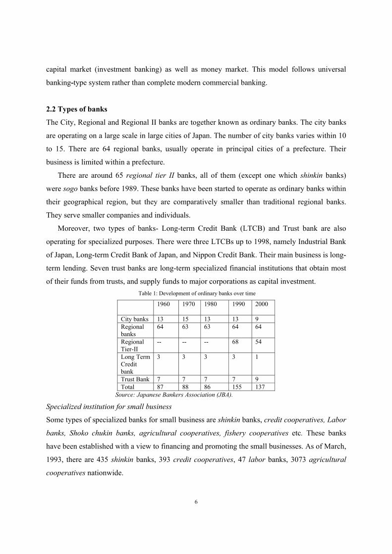
2.2 Types of banks
The City, Regional and Regional II banks are together known as ordinary banks. The city banks
are operating on a large scale in large cities of Japan. The number of city banks varies within 10
to 15. There are 64 regional banks, usually operate in principal cities of a prefecture. Their
business is limited within a prefecture.
There are around 65 regional tier II banks, all of them (except one which shinkin banks)
were sogo banks before 1989. These banks have been started to operate as ordinary banks within
their geographical region, but they are comparatively smaller than traditional regional banks.
They serve smaller companies and individuals.
Moreover, two types of banks- Long-term Credit Bank (LTCB) and Trust bank are also
operating for specialized purposes. There were three LTCBs up to 1998, namely Industrial Bank
of Japan, Long-term Credit Bank of Japan, and Nippon Credit Bank. Their main business is long-
term lending. Seven trust banks are long-term specialized financial institutions that obtain most
of their funds from trusts, and supply funds to major corporations as capital investment.
Table 1: Development of ordinary banks over time
1960 1970 1980 1990
2000
City banks 13 15 13 13 9
Regional
banks
64 63 63 64 64
Regional
Tier-II
-- -- -- 68 54
Long Term
Credit
bank
3 3 3 3 1
Trust Bank 7 7 7 7 9
Total 87 88 86 155 137
Source: Japanese Bankers Association (JBA).
Specialized institution for small business
Some types of specialized banks for small business are shinkin banks, credit cooperatives, Labor
banks, Shoko chukin banks, agricultural cooperatives, fishery cooperatives etc. These banks
have been established with a view to financing and promoting the small businesses. As of March,
1993, there are 435 shinkin banks, 393 credit cooperatives, 47 labor banks, 3073 agricultural
cooperatives nationwide.
7
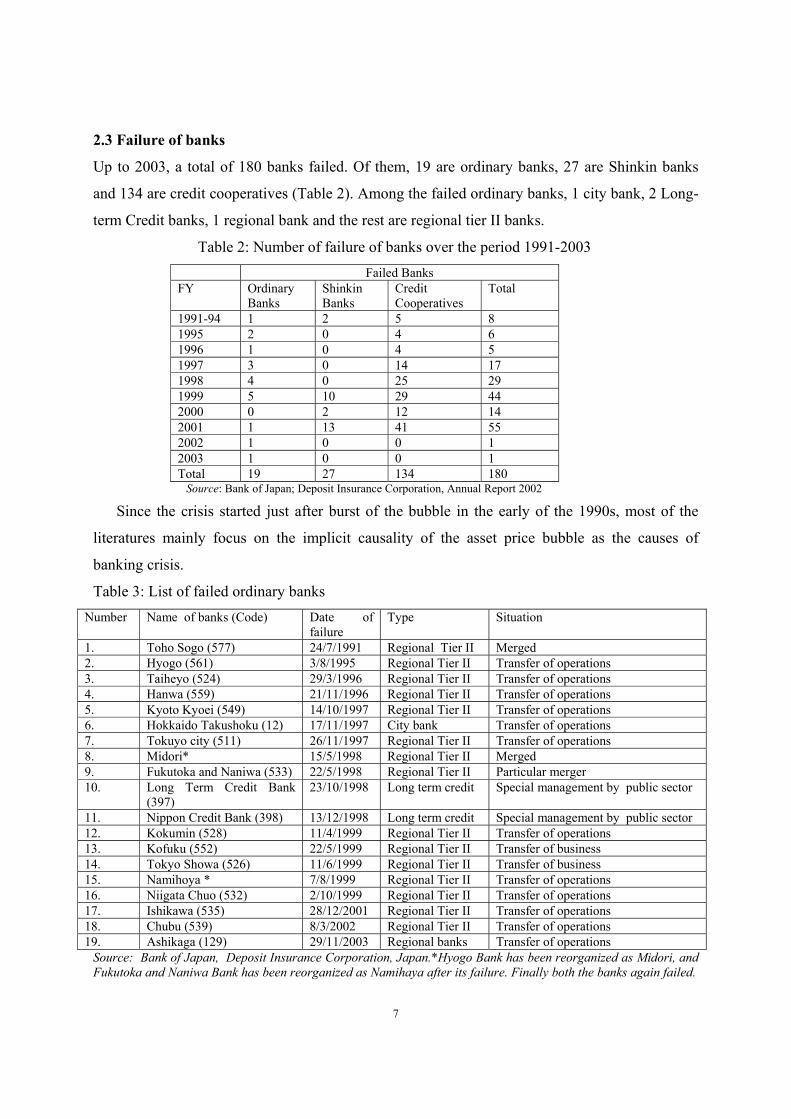
2.3 Failure of banks
Up to 2003, a total of 180 banks failed. Of them, 19 are ordinary banks, 27 are Shinkin banks
and 134 are credit cooperatives (Table 2). Among the failed ordinary banks, 1 city bank, 2 Long-
term Credit banks, 1 regional bank and the rest are regional tier II banks.
Table 2: Number of failure of banks over the period 1991-2003
Failed Banks
FY Ordinary
Banks
Shinkin
Banks
Credit
Cooperatives
Total
1991-94 1 2 5 8
1995 2 0 4 6
1996 1 0 4 5
1997 3 0 14 17
1998 4 0 25 29
1999 5 10 29 44
2000 0 2 12 14
2001 1 13 41 55
2002 1 0 0 1
2003 1 0 0 1
Total 19 27 134 180 Source: Bank of Japan; Deposit Insurance Corporation, Annual Report 2002
Since the crisis started just after burst of the bubble in the early of the 1990s, most of the
literatures mainly focus on the implicit causality of the asset price bubble as the causes of
banking crisis.
Table 3: List of failed ordinary banks
Number Name of banks (Code) Date of
failure
Type Situation
1. Toho Sogo (577) 24/7/1991 Regional Tier II Merged
2. Hyogo (561) 3/8/1995 Regional Tier II Transfer of operations
3. Taiheyo (524) 29/3/1996 Regional Tier II Transfer of operations
4. Hanwa (559) 21/11/1996 Regional Tier II Transfer of operations
5. Kyoto Kyoei (549) 14/10/1997 Regional Tier II Transfer of operations
6. Hokkaido Takushoku (12) 17/11/1997 City bank Transfer of operations
7. Tokuyo city (511) 26/11/1997 Regional Tier II Transfer of operations
8. Midori* 15/5/1998 Regional Tier II Merged
9. Fukutoka and Naniwa (533) 22/5/1998 Regional Tier II Particular merger
10. Long Term Credit Bank
(397)
23/10/1998 Long term credit Special management by public sector
11. Nippon Credit Bank (398) 13/12/1998 Long term credit Special management by public sector
12. Kokumin (528) 11/4/1999 Regional Tier II Transfer of operations
13. Kofuku (552) 22/5/1999 Regional Tier II Transfer of business
14. Tokyo Showa (526) 11/6/1999 Regional Tier II Transfer of business
15. Namihoya * 7/8/1999 Regional Tier II Transfer of operations
16. Niigata Chuo (532) 2/10/1999 Regional Tier II Transfer of operations
17. Ishikawa (535) 28/12/2001 Regional Tier II Transfer of operations
18. Chubu (539) 8/3/2002 Regional Tier II Transfer of operations
19. Ashikaga (129) 29/11/2003 Regional banks Transfer of operations
Source: Bank of Japan, Deposit Insurance Corporation, Japan.*Hyogo Bank has been reorganized as Midori, and
Fukutoka and Naniwa Bank has been reorganized as Namihaya after its failure. Finally both the banks again failed.
8
Although most of the failed banks have been either merged or recapitalized, it is still not
certain that the crisis has been finished. If the crisis is related to only monetary easing and bubble
economy of the 1980s, the crisis should have to be ended earlier. If the crisis is inherent in
banking operations and management efficiency, the issue is worrisome. This is the focus of this
paper.
3. Potential determinants of banking crisis
The prospects of failure of banks can be explained by analyzing the following characteristics
of the banking business: (i) asset risk, (ii) capital adequacy, (iii) liquidity, (iv) management and
operating efficiency, and (v) earnings. Banks usually are threatened with failure because of
losses on assets; on the other hand, liquidity, capital adequacy and earnings measure the ability
of a bank to open in spite of these losses. Capital adequacy and earnings allow losses to be offset
by current or past income (Mishkin, 2003). Some argue that ample liquidity after the 1985 Plaza
Accord provided the funds for speculation (Arayama and Mourdoukoutas, 2000), but our
analysis shows that only the city banks had had high liquidity after the Plaza accord and except
regional banks tier II, other banks liquidity position over the time period has not been found
significantly different (Table B in Appendix-I).
Generally, each of these above five characteristics may have influence on banks prospect of
failure. Asset quality is important for determining the current and future profitability of the bank;
it deteriorates with the significant increase of non-performing loan. On the other hand, capital
adequacy can reduce risk of failure and absorb losses. Capital acts as buffer against loan losses, it
may prevent the failure whose customers default on their loans. According to Nelson (1977), the
probability of failure is a function of current level of capital, and the estimated mean and
variance of earnings and charge-offs.
Management and operating efficiency of the Japanese banks is a widely discussed topic.
Management sets the profitability objectives of bank and determine loan portfolio by proper
lending risk analysis. Earning is measured by either of the ratios ROA, ROE or Net Interest
Margin. A low ROA may either be due to conservative lending and investment policies or
excessive operating expenses. Regarding low profitability of Japanese banks, one view is that
banks expanded their sizes and assets that required high operating expense which have negative
effect on profit.
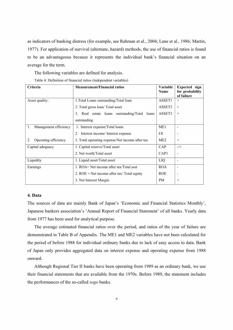
In this paper, an attempt has been made to find the determinants of banking crisis by
analyzing financial ratios. In Table 4, we define some financial ratios that are widely considered
9
as indicators of banking distress (for example, see Rahman et al., 2004; Lane et al., 1986; Martin,
1977). For application of survival (alternate, hazard) methods, the use of financial ratios is found
to be an advantageous because it represents the individual bank’s financial situation on an
average for the term.
The following variables are defined for analysis.
Table 4: Definition of financial ratios (independent variables)
Criteria Measurement/Financial ratios Variable
Name
Expected sign
for probability
of failure
Asset quality: 1.Total Loans outstanding/Total loan
2. Total gross loan/ Total asset
3. Real estate loans outstanding/Total loans
outstanding
ASSET1
ASSET2
ASSET3
+
+
+
1. Management efficiency
2. Operating efficiency
1. Interest expense/Total loans
2. Interest income/ Interest expense
3. Total operating expense/Net income after tax
ME1
I/E
ME2
-
-
+
Capital adequacy 1. Capital reserve/Total asset
2. Net worth/Total asset
CAP
CAP1
-/+
-
Liquidity 1. Liquid asset/Total asset LIQ -
Earnings 1. ROA= Net income after tax/Total asst
2. ROE = Net income after tax/ Total equity
3. Net Interest Margin
ROA
ROE
PM
-
-
+
4. Data
The sources of data are mainly Bank of Japan’s ‘Economic and Financial Statistics Monthly’,
Japanese bankers association’s ‘Annual Report of Financial Statement’ of all banks. Yearly data
from 1977 has been used for analytical purpose.
The average estimated financial ratios over the period, and ratios of the year of failure are
demonstrated in Table B of Appendix. The ME1 and ME2 variables have not been calculated for
the period of before 1988 for individual ordinary banks due to lack of easy access to data. Bank
of Japan only provides aggregated data on interest expense and operating expense from 1988
onward.
Although Regional Tier II banks have been operating from 1989 as an ordinary bank, we use
their financial statements that are available from the 1970s. Before 1989, the statement includes
the performances of the so-called sogo banks.
10
The details of data management for the application of survival models are discussed in
respective sections.
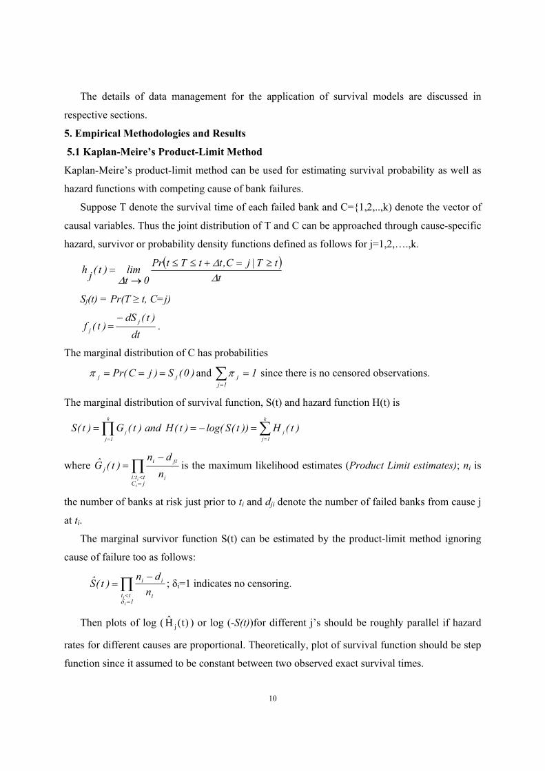
5. Empirical Methodologies and Results
5.1 Kaplan-Meire’s Product-Limit Method
Kaplan-Meire’s product-limit method can be used for estimating survival probability as well as
hazard functions with competing cause of bank failures.
Suppose T denote the survival time of each failed bank and C={1,2,..,k) denote the vector of
causal variables. Thus the joint distribution of T and C can be approached through cause-specific
hazard, survivor or probability density functions defined as follows for j=1,2,….,k.
( )t
tT|jC,ttTtPr
0tlim)t(
jh
∆∆
∆
≥=+≤≤
→=
Sj(t) = Pr(T ≥ t, C=j)
dt
)t(dS)t(f
j
j
−= .
The marginal distribution of C has probabilities
)0(S)jCPr( jj ===π and ∑=
=1j
j 1π since there is no censored observations.
The marginal distribution of survival function, S(t) and hazard function H(t) is
∑∏==
=−==k
1j
j
k
1j
j)t(H))t(Slog()t(Hand)t(G)t(S
where ∏=<
−=
jCtt:i i
jii
j
i
in
dn)t(G is the maximum likelihood estimates (Product Limit estimates); ni is
the number of banks at risk just prior to ti and dji denote the number of failed banks from cause j
at ti.
The marginal survivor function S(t) can be estimated by the product-limit method ignoring
cause of failure too as follows:
∏=<
−=
1tt i
ii
i
in
dn)t(S
δ
; δi=1 indicates no censoring.
Then plots of log ( )t(H j ) or log (-S(t))for different j’s should be roughly parallel if hazard
rates for different causes are proportional. Theoretically, plot of survival function should be step
function since it assumed to be constant between two observed exact survival times.
11
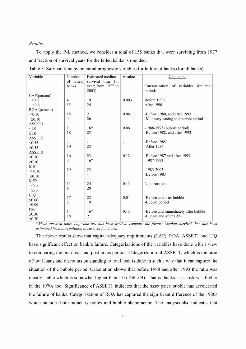
Results:
To apply the P-L method, we consider a total of 155 banks that were surviving from 1977
and fraction of survival years for the failed banks is rounded.
Table 5: Survival time by potential prognostic variables for failure of banks (for all banks).
Variable Number
of failed
banks
Estimated median
survival time (in
year; from 1977 to
2003)
p-value Comments
Categorization of variables for the
period:
CAP(percent)
<0.8
≥0.8
ROA (percent)
<0.10
≥0.10
ASSET1
<1.0
≥1.0
ASSET2
<0.55
≥0.55
ASSET3
<0.10
≥0.10
ME1
< 0.10
≥0.10
ME2
<30
≥30
LIQ
≤0.06
>0.06
PM
≤0.30
>0.30
4
15
15
4
1
18
-
19
16
3
19
-
11
8
17
2
1
18
19
24
21
26
16*
23
-
23
23
16*
23
-
24
20
23
19
16*
21
0.003
0.06
0.06
-
0.12
-
0.13
0.01
0.13
Before 1990
After 1990
-Before 1980, and after 1993
-Monetary easing and bubble period
-1988-1993 (bubble period)
-Before 1988, and after 1993
-Before 1985
-After 1985
-Before 1987 and after 1993
-1987-1993
-1983-2003
-Before 1983
No clear trend
-Before and after bubble
-Bubble period
-Before and immediately after bubble
-Bubble and after 1993
*Mean survival time; Log-rank test has been used to compare the factor; Median survival time has been
estimated from interpolation of survival functions.
The above results show that capital adequacy requirements (CAP), ROA, ASSET1 and LIQ
have significant effect on bank’s failure. Categorizations of the variables have done with a view
to comparing the pre-crisis and post-crisis period. Categorization of ASSET1, which is the ratio
of total loans and discounts outstanding to total loan is done in such a way that it can capture the
situation of the bubble period. Calculation shows that before 1988 and after 1993 the ratio was
mostly stable which is somewhat higher than 1.0 (Table B). That is, banks asset risk was higher
in the 1970s too. Significance of ASSET1 indicates that the asset price bubble has accelerated
the failure of banks. Categorization of ROA has captured the significant difference of the 1980s
which includes both monetary policy and bubble phenomenon. The analysis also indicates that
12
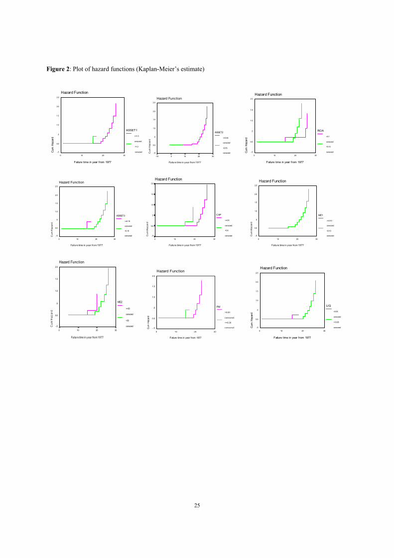
higher value of ASSET1, ASSET2 and CAP and lower value of ROA, ASSET3, ME1, LIQ
increases the probability of failure of the Japanese banks (Figure 2). The significance of low
ROA (as it is evident in the 1970s too) to the failure therefore provides a warning of future crisis.
Moreover, higher value of ASSET3, ME2, LIQ and lower value of CAP, ROA, and ASSET1
decreases the median survival time (Table 5). This finding indicates that emergence and burst of
the bubble in the late 1980s led to an early crisis, the estimated median survival time also
indicates that without the shock it would take around 5-7 years more to reach the crisis situation.
All the variables are used to compare the pre and post-bubble period. Most of the banks
failed mostly with the same financial condition of the pre-bubble period. Therefore we may
conclude that the situation of banks in the 1970s was a warning for crisis and the situation has
been accelerated to an early crisis by the burst of the bubble.
However, examination of each variable by PL estimate can give preliminary idea of which
variables might be of prognostic importance. The simultaneous effect of the variables must be
analyzed by an appropriate multivariate statistical method to determine the relative importance of
each.
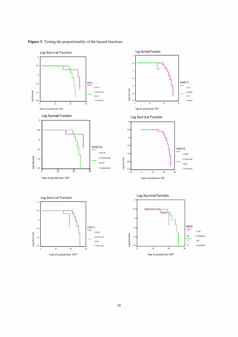
For this purpose, we discuss the Cox’s (1972) proportional hazards model in the following
section. The assumption of this model is that the hazards for different strata of each independent
(or prognostic) variable are proportional over time. This assumption is verified graphically by
plotting log[-S(t)] versus t for two subgroups of each variable(Figure-3). The two almost
parallel curves indicate that the hazards of failure of banks are proportional. Therefore, it is
justified to use the proportional hazards model.
5.2 Proportional Hazards Model
Let T be a continuous variable representing a bank’s survival time and Z= (Z1, Z2,…..,Zp) be
a known vector of regression coefficients. With the assumption that different bank has hazard
functions which are proportional to each other and independent of time, the Cox’s (1972)
proportional hazard model can be defined as
βλλ z
0e)t()z,t( =
( )( ) MEROAASSETCAPzt
z,tlog 4
p
1j
321jij
0
i βββββλλ ∑
=
+++==⇒
where λ0(t) is only a function of time t and is known as base-line hazard rate which represents
how the risk changes with time. The advantage of this model is that it does not require any
distributional assumptions (for more details, see Cox(1972)).
13
The model has a partial likelihood function in which the only parameters are the coefficients
associated with covariates. However, statistical inference based on the partial likelihood has
asymptotic properties. The partial likelihood takes different forms based on the presence or
absence of tied observations. Newton-Raphson Iterative procedure is required to get the
estimates.
The underlying assumptions of the hazards model are to assign the characteristics of the
subjects (e.g. banks) measured at start-point or end-point or any other specified time-point to the
failure (or survival) time of the subjects in a prospective study. Nonetheless, there is no clear-cut
rule about the time-specification of the covariates (or, explanatory variables), but the
interpretation must depends on the specification (Kiefer, 1988)3. In this paper, I have examined
different time-specifications of the covariates for the PH model, such as the start-point (1990),
end-point (2003), and the average of the whole period. The use of aggregate average ratios of the
whole period for the non-failed banks and specific aggregate ratio of the year of failure for failed
banks has been found effective in analyzing the causes of failure of the Japanese banks. Only the
ordinary banks have been considered for analysis as they are big in size.
I consider all covariates as time dependent except CAP and CAP1 since it is a legal
requirement. I consider the 1554 banks that were surviving at the beginning of 1990s and there
were no tied observations. Since the financial ratios vary for different types of banks, stratified
Cox’s proportional hazards model has been used. The survival time has been calculated for the
period 1990 to 2003.
In the first attempt, I have fitted stratified Cox’s PH model by analyzing the ratios ASSET2,
CAP1, I/E, ME1, ME2, ROA of the base-line year 1990 as covariates for the existing154 banks,
of which 17 have failed. Among the estimated coefficients, only interest income over interest
expense has been found significant5 as a cause of future bank-failure (Table A in Appendix). The
other variables have not been found significant, probably because of the fact that only one year’s
data is not enough to capture the long-term time series trend.
Therefore in another attempt I revitalize the assumption to estimate the Cox’s regression
coefficient. I assume that the failed banks represent the specific ratio of the year of failure, and
3 Kiefer (1988) also mentioned that assigning economic meanings to coefficients is a matter of modeling and
judicious use of prior information. 4 The number of banks varies over time due to merging or newly emergence. For aggregate data analysis, I consider
155 banks; while for 1990, data of existing 154 banks has been analyzed. So far in survival analysis, this trivial
variation in number of banks does not create any significant difference. 5 ME1 and I/E are highly correlated, and in absence of I/E all other variables are not significant. But I/E has been
found highly significant in all situations.
14
the rest non-failed banks continue with the average ratio for the period 1990-2003. From Table C
in Appendix-II, it can be easily seen that the average ratios of 1990-2003 are mostly comparable
with that of pre-1990, i.e. it maintains the long term trend pattern. A more detailed explanation
about data analysis has been provided in Appendix-II. Therefore, the assumption makes it
possible to compare the failed banks’ financial situation with that of pre-crisis period’s situation
(see Table B in Appendix-I) without losing generality of the assumption of PH model. This
specification also makes it possible to compare with that of end-point (e.g. 2003) ratios.
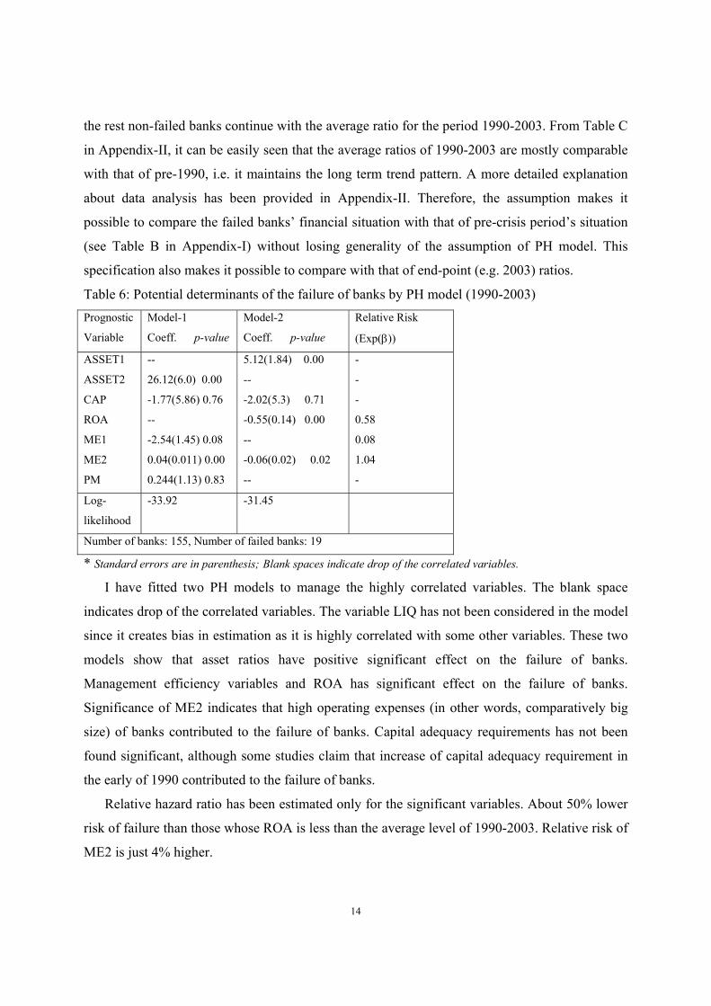
Table 6: Potential determinants of the failure of banks by PH model (1990-2003)
Prognostic
Variable
Model-1
Coeff. p-value
Model-2
Coeff. p-value
Relative Risk
(Exp(β))
ASSET1
ASSET2
CAP
ROA
ME1
ME2
PM
--
26.12(6.0) 0.00
-1.77(5.86) 0.76
--
-2.54(1.45) 0.08
0.04(0.011) 0.00
0.244(1.13) 0.83
5.12(1.84) 0.00
--
-2.02(5.3) 0.71
-0.55(0.14) 0.00
--
-0.06(0.02) 0.02
--
-
-
-
0.58
0.08
1.04
-
Log-
likelihood
-33.92 -31.45
Number of banks: 155, Number of failed banks: 19
* Standard errors are in parenthesis; Blank spaces indicate drop of the correlated variables.
I have fitted two PH models to manage the highly correlated variables. The blank space
indicates drop of the correlated variables. The variable LIQ has not been considered in the model
since it creates bias in estimation as it is highly correlated with some other variables. These two
models show that asset ratios have positive significant effect on the failure of banks.
Management efficiency variables and ROA has significant effect on the failure of banks.
Significance of ME2 indicates that high operating expenses (in other words, comparatively big
size) of banks contributed to the failure of banks. Capital adequacy requirements has not been
found significant, although some studies claim that increase of capital adequacy requirement in
the early of 1990 contributed to the failure of banks.
Relative hazard ratio has been estimated only for the significant variables. About 50% lower
risk of failure than those whose ROA is less than the average level of 1990-2003. Relative risk of
ME2 is just 4% higher.
15
Since the above interpretations are based on the specification that the ratios are higher (or
lower) for survived banks than the failed banks, these ratios together form a set of indicators for
the failure of the Japanese banks. Therefore increase or decrease of ratios to a certain level may
contribute to the failure of banks (Table C).
5.3 Accelerated Failure Time (AFT) Model
The AFT model of survival time (Cox, 1972) assumes that the relationship of logarithm of
survival time T and covariates is linear and can be expressed as
σεββ ++= ∑=
p
1j
jij0 Z)Tlog(
where Zj’s are the covariates, βj’s be the coefficients, σ (σ>0) is an unknown scale parameter,
and ε, the error term, is a random variable with known forms of density function g(ε) and
survivorship function G(ε). Thus the survival is dependent on both the covariate and an
underlying distribution g. This model shows the covariate Z either ‘accelerates’ or ‘decelerates’
the survival time or time to failure.
Again assume that εi follows logistic regression model with density function
[ ]2)exp(1
)exp()(g
εεε
+=
and survivorship function
)exp(1
1)(G
εε
+= .
Hence the model resembles the properties of log-logistic model.
Suppose S(t, β) denote the probability of surviving longer than t, then [ ]ββ ,t(S1),t(S −
gives the odds of surviving longer than t. Let ORi and ORj denote the odds of surviving larger
than t for specific conditions i and j, respectively. The logarithm of odds ratio is thus
∑=
−=p
1k
kjkik
j
i )xx(1
OR
ORlog β
σ,
and, the ratio is independent of time. Therefore, the log-logistic regression model is a
proportional odds model, rather than a proportional hazards model. Opposite sign of PH model is
expected in this case.
Therefore, we define the model,
σεααααα +++++= MEROAASSETCAPTlog 43210i
16
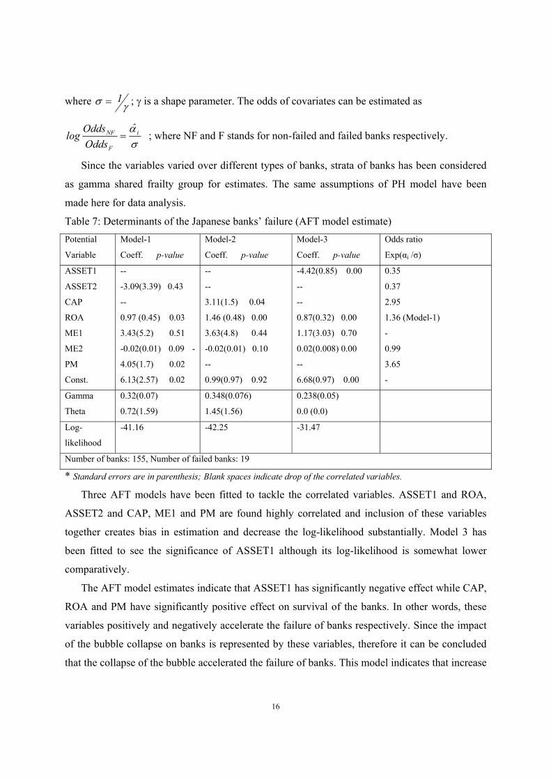
where γσ 1= ; γ is a shape parameter. The odds of covariates can be estimated as
σα i
F
NFˆ
Odds
Oddslog = ; where NF and F stands for non-failed and failed banks respectively.
Since the variables varied over different types of banks, strata of banks has been considered
as gamma shared frailty group for estimates. The same assumptions of PH model have been
made here for data analysis.
Table 7: Determinants of the Japanese banks’ failure (AFT model estimate)
Potential
Variable
Model-1
Coeff. p-value
Model-2
Coeff. p-value
Model-3
Coeff. p-value
Odds ratio
Exp(αi /σ)
ASSET1
ASSET2
CAP
ROA
ME1
ME2
PM
Const.
--
-3.09(3.39) 0.43
--
0.97 (0.45) 0.03
3.43(5.2) 0.51
-0.02(0.01) 0.09 -
4.05(1.7) 0.02
6.13(2.57) 0.02
--
--
3.11(1.5) 0.04
1.46 (0.48) 0.00
3.63(4.8) 0.44
-0.02(0.01) 0.10
--
0.99(0.97) 0.92
-4.42(0.85) 0.00
--
--
0.87(0.32) 0.00
1.17(3.03) 0.70
0.02(0.008) 0.00
--
6.68(0.97) 0.00
0.35
0.37
2.95
1.36 (Model-1)
-
0.99
3.65
-
Gamma
Theta
0.32(0.07)
0.72(1.59)
0.348(0.076)
1.45(1.56)
0.238(0.05)
0.0 (0.0)
Log-
likelihood
-41.16 -42.25 -31.47
Number of banks: 155, Number of failed banks: 19
* Standard errors are in parenthesis; Blank spaces indicate drop of the correlated variables.
Three AFT models have been fitted to tackle the correlated variables. ASSET1 and ROA,
ASSET2 and CAP, ME1 and PM are found highly correlated and inclusion of these variables
together creates bias in estimation and decrease the log-likelihood substantially. Model 3 has
been fitted to see the significance of ASSET1 although its log-likelihood is somewhat lower
comparatively.
The AFT model estimates indicate that ASSET1 has significantly negative effect while CAP,
ROA and PM have significantly positive effect on survival of the banks. In other words, these
variables positively and negatively accelerate the failure of banks respectively. Since the impact
of the bubble collapse on banks is represented by these variables, therefore it can be concluded
that the collapse of the bubble accelerated the failure of banks. This model indicates that increase
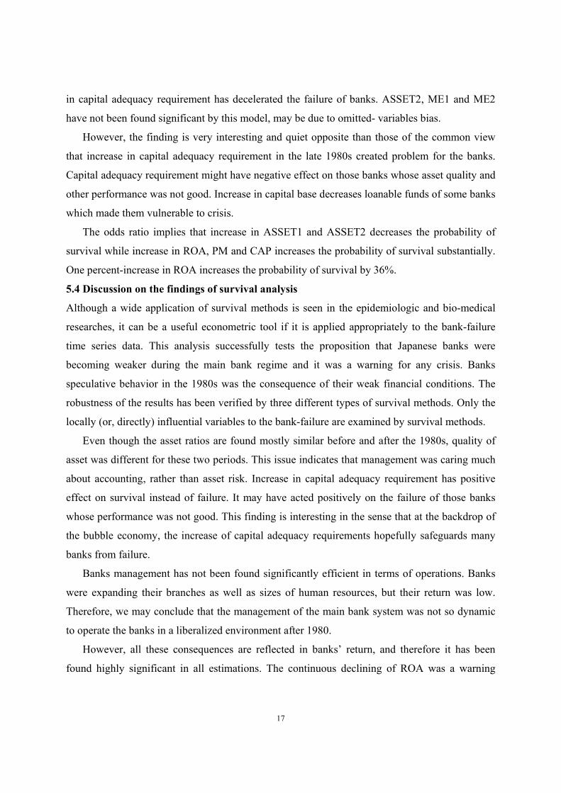
17
in capital adequacy requirement has decelerated the failure of banks. ASSET2, ME1 and ME2
have not been found significant by this model, may be due to omitted- variables bias.
However, the finding is very interesting and quiet opposite than those of the common view
that increase in capital adequacy requirement in the late 1980s created problem for the banks.
Capital adequacy requirement might have negative effect on those banks whose asset quality and
other performance was not good. Increase in capital base decreases loanable funds of some banks
which made them vulnerable to crisis.
The odds ratio implies that increase in ASSET1 and ASSET2 decreases the probability of
survival while increase in ROA, PM and CAP increases the probability of survival substantially.
One percent-increase in ROA increases the probability of survival by 36%.
5.4 Discussion on the findings of survival analysis
Although a wide application of survival methods is seen in the epidemiologic and bio-medical
researches, it can be a useful econometric tool if it is applied appropriately to the bank-failure
time series data. This analysis successfully tests the proposition that Japanese banks were
becoming weaker during the main bank regime and it was a warning for any crisis. Banks
speculative behavior in the 1980s was the consequence of their weak financial conditions. The
robustness of the results has been verified by three different types of survival methods. Only the
locally (or, directly) influential variables to the bank-failure are examined by survival methods.
Even though the asset ratios are found mostly similar before and after the 1980s, quality of
asset was different for these two periods. This issue indicates that management was caring much
about accounting, rather than asset risk. Increase in capital adequacy requirement has positive
effect on survival instead of failure. It may have acted positively on the failure of those banks
whose performance was not good. This finding is interesting in the sense that at the backdrop of
the bubble economy, the increase of capital adequacy requirements hopefully safeguards many
banks from failure.
Banks management has not been found significantly efficient in terms of operations. Banks
were expanding their branches as well as sizes of human resources, but their return was low.
Therefore, we may conclude that the management of the main bank system was not so dynamic
to operate the banks in a liberalized environment after 1980.
However, all these consequences are reflected in banks’ return, and therefore it has been
found highly significant in all estimations. The continuous declining of ROA was a warning
18
signal for banking crisis. Therefore, it is necessary to identify the potential determinants of low
profitability of the Japanese banks.
For survival analysis, either of the computer packages STATA, SAS, SPSS, or BMDP can be
used.
6. Banks profitability and determinants
Highly significance of low ROA on bank’s failure necessitates the analysis of declining
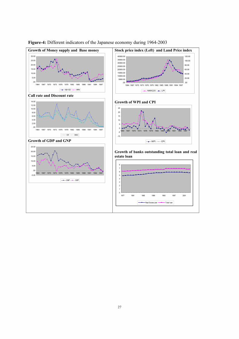
profitability of Japanese banks. Figure-1 shows that the declining trend of profitability of
Japanese banks continued from 1970 except during the asset price bubble and monetary easing
period in the 1980s, and Figure 4 demonstrates the trend of different macroeconomic indicators.
Some authors argue that the low profitability during the sluggish economy was due to poor
macroeconomic conditions. The economy at that time lacks enough profitable investments, or
deflation and near-zero interest rate prevents banks earning from fair return on their investment.
The usual question is why banks’ profitability was declining during the high economic growth
period of Japan? Were the banks ever caring about their declining trend of profit? It is important
to analyze the declining trend of profits to avert any future collapse of the Japanese banks.
One important argument is that Japanese banks are unable or unwilling to exploit profitable
lending opportunities. During the main bank regime, banks were caring much about market share
rather than profit (Yoshino and Sakakibara, 2002). Some pundits argue that Japanese economic
growth has been achieved at the expense of banks’ profit.
We may guess some other reasons that might contribute to the Japanese banks’ low profit
during high growth period. Sometimes, to meet up the enterprise groups’ excess demand for
money, bank borrowed from call money market with high interest rate and lent it to its affiliated
firm with the existing (usually lower) interest rate. This preferential loan might have impact on
declining trend of banks’ profit. Again, borrowing short and lending long created a mismatch in
the financial system as there are some maturity gap (exact data are not available) between the
deposit fund and loan portfolio in the Japanese banks (Ito, 1992; Smith, D.C., 2002). This
structural weaknesses affected profitability of the main bank system of Japan. Moreover, lending
risk analysis could be biased due to the presence of directors of enterprise firms in banks, which
pinpoints inefficiency of the management. Also we cannot deny the possibility of window
dressing6 in bank’s profit; if it is so, the actual profit of banks was lower than the reported one.
6Bank sometimes manipulate their financial statements to show a inflated position of their performance by taking
favor from their own enterprise group. This unfair means is termed as Window Dressing. It could be a very difficult
task to get proper information on window dressing in Japan.
19
Caves and Uekusa (1976, pp. 72-83) showed that group membership decline a firm’s rate of
profit; so does banks profit. Therefore preferential loan, window dressing, window guidance etc.
trigger the efficiency of the management, in other words, the problems of corporate governance.
Therefore these factors may be the determinants of profit during the main bank regime. However,
it is difficult to find appropriate proxy to measure the effect of some of the above variables.
The Granger causality test and cointegration test have been performed to identify the
determinants of low profitability of banks. The variables used are: log of asset (LASSET) as a
proxy for size, call rate minus discount rate (DINT), interest income/interest expense (I/E) and
ME1 as a proxy for management efficiency as well as a proxy for preferential loan, growth of
money supply (M2CD), growth of land price index (LPIND), net interest margin (PM), operating
efficiency (ME2), uncollateralized call rate (CR), discount rate (DR), GDP growth (GDP) and
households savings rate.
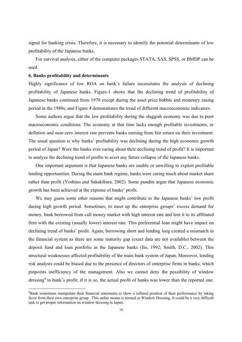
6.1 Cointegration and Granger causality test
To test for long-run determinants of banks ROA, we first present in Table 8 unit root tests on
the yearly data of all domestically licensed banks from 1977 to 2003. We are unable to reject the
existence of a unit root for all the series except ME2 and DINT.
Table 8: Unit-root test (Dickey-Fuller statistic)
Variable Dickey-Fuller
Test Statistic
Variable Dickey-Fuller
Test Statistic
ROA
PM
I/E
DINT
ME1
ME2
GDP
-1.25
-2.94
1.92
-4.73*
-2.38
-5.17*
-2.51
LPIND
M2CD
HHSR
CR
DR
LASSET
-0.524
-2.58
-1.75
-3.15
-2.78
0.76
Note: The unit-root tests include both trend and intercept.
*indicates rejection of null hypothesis at 1% level of significance.
I next test for cointegration between ROA and these variables. Table 9 shows the test statistics
for the null hypothesis of no cointegration between ROA and other variables. We find
cointegration between ROA and I/E, growth of money supply, log of total asset (LASSET),
growth of land price index (LPIND), ME1, household saving rate (HHSR), GDP growth rate and
discount rate. The result indicates the existence of long-run relationship of this variables and
ROA.
20
Table 9: Test for cointegration of ROA and the other variables
Variable Likelihood
Ratio
Variable Likelihood
Ratio
LASSET
LPIND
M2CD
HHSR
CR
33.77*
30.63*
33.74*
33.02*
22.12
I/E
ME1
PM
DR
GDP
31.75*
55.59*
19.02
27.07**
29.88**
Notes: Test allows intercept and linear deterministic trend in the data. The
critical value is 25.32 for 5% and 30.45 for 1% significance level.
* and ** indicates rejection of null hypothesis at 1% and 5% level respectively.
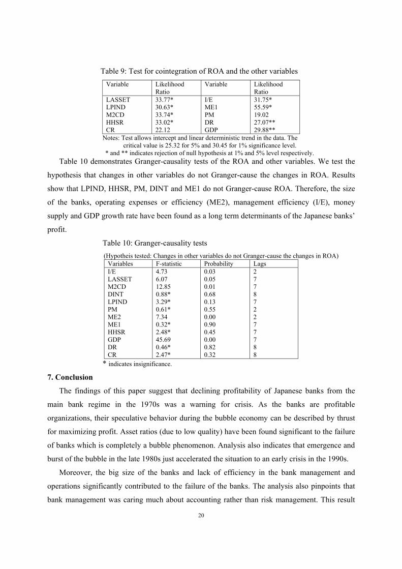
Table 10 demonstrates Granger-causality tests of the ROA and other variables. We test the
hypothesis that changes in other variables do not Granger-cause the changes in ROA. Results
show that LPIND, HHSR, PM, DINT and ME1 do not Granger-cause ROA. Therefore, the size
of the banks, operating expenses or efficiency (ME2), management efficiency (I/E), money
supply and GDP growth rate have been found as a long term determinants of the Japanese banks’
profit.
Table 10: Granger-causality tests
(Hypotheis tested: Changes in other variables do not Granger-cause the changes in ROA)
Variables F-statistic Probability Lags
I/E
LASSET
M2CD
DINT
LPIND
PM
ME2
ME1
HHSR
GDP
DR
CR
4.73
6.07
12.85
0.88*
3.29*
0.61*
7.34
0.32*
2.48*
45.69
0.46*
2.47*
0.03
0.05
0.01
0.68
0.13
0.55
0.00
0.90
0.45
0.00
0.82
0.32
2
7
7
8
7
2
2
7
7
7
8
8
* indicates insignificance.
7. Conclusion
The findings of this paper suggest that declining profitability of Japanese banks from the
main bank regime in the 1970s was a warning for crisis. As the banks are profitable
organizations, their speculative behavior during the bubble economy can be described by thrust
for maximizing profit. Asset ratios (due to low quality) have been found significant to the failure
of banks which is completely a bubble phenomenon. Analysis also indicates that emergence and
burst of the bubble in the late 1980s just accelerated the situation to an early crisis in the 1990s.
Moreover, the big size of the banks and lack of efficiency in the bank management and
operations significantly contributed to the failure of the banks. The analysis also pinpoints that
bank management was caring much about accounting rather than risk management. This result
21
indicates that expansion of the sizes of the banks have been done without caring much about
return. The low return ultimately makes the banks vulnerable to crisis.
As a part of long run determinants of profit, a large number of variables have been checked
with cointegration and Granger-causality tests. Banks size, ratio of interest income over interest
expense, operating efficiency ratio, GDP growth and growth of money supply have been
identified as significant long term determinants of profit.
The use of survival models to the Japanese banking failure data is quiet new to my
knowledge, and the findings are interesting and robust. The findings have important policy
implications too. Since the crisis occurring variables are inherently related to baking operations
and management, we can not overrule the future possibility of Japanese banking crisis unless or
until the corporate governance has been improved significantly.
Acknowledgment
I wish to thank Profs. Yoichi Okita, Kenichi Ohno, Kaliappa Kalirajan and Futoshi Yamauchi for
their helpful comments and cooperation. I also would like to express my gratitude to Farhana
Rafiq, Anwar Sansui, K. Kanda and Masuda for their cooperation in collecting and compiling
data.
References:
Aoki, M., and H. Patrick, 1994. The Japanese main bank system: Its relevance for developing
and transforming economies, Oxford University Press.
Arayama, Yuko and Panos Mourdoukoutas, 2000. The rise and fall of abacus banking in Japan
and China. Quorum Books.
Cargill, Thomas, 2000. What caused Japan’s banking crisis? In Takeo Hoshi and Hugh Patrick,
eds. Crisis and Change in the Japanese Financial System. Kluwer Academic Publisher, 37-58.
Cargll, Thomas F. and Shoichi Royama (1988): The transition of finance in Japan and the U.S.,
Stanford CA, Hoover Press.
Caves R. and M. Uekusa (1976) Industrial organization in Japan. Brookings Institution.
Cox, D. R. (1972). Regression models and life tables (with discussion). J. R. Statist. Soc. B, 34,
187-220.
Hoshi T., A. Kashyap, and D. Scharfstein (1991): Corporate structure, liquidity and investment:
Evidence from Japanese Industrial groups. Quarterly Journal of Economics 106, February, 33-60.
Hoshi, Takeo and Anil Kashyap, 1999. The Japanese banking crisis: where did it come from and
how will it end? NBER working paper no. 7250, National Bureau of Economic Research.
Hoshi, Takeo, 2001. What happened to Japanese banks? Monetary and Economic Studies,
February, Bank of Japan.
Ito T. (1992): The Japanese Economy, MIT Press.
22
Kiefer, Nicholas M., 1988. Economic duration data and hazard functions. Journal of Economic
Literature, 26, pp. 646-679.
Lane, W. R., S. W. Looney and J. W. Wansley, 1986. An application of the Cox proportional
hazards model to bank failure. Journal of Banking and Finance10, 511-531.
Martin, Daniel, 1977.Early warning of bank failure: A logit regression approach. Journal of
Banking and Finance 1, 249-276.
Mishkin, S. Frederic, 2003. The economics of money, banking and financial markets. Addison-
Wesley, 3rd
Edition.
Nelson, R. W., 1977. Optimal capital policy of the commercial banking firm in relation to
expectations concerning loan losses. Federal Reserve Bank of New York working paper.
Okabe, M. (2001): Are cross-shareholding of Japanese corporations dissolving? Evolution and
implications, Nissan Occasional Paper Series No. 33.
Okina, K., et al., 2001. The asset price bubble and monetary policy: Japan’s experience in the
late 1980s and the lessons. Monetary and Economic Studies, February, Bank of Japan.
Rahman, Shahidur, et al., 2004. Identifying financial distress indicators of selected banks in Asia.
Asian Economic Journal 18(1), 45-57.
Smith, David C. (2002). Loans to Japanese borrowers. Pacific Basin Working Paper Series,
PB02-11.
Suzuki Y.(1980): Money and Banking in Contemporary Japan. Yale University Press.
Suzuki Y. (1987): The Japanese Financial System, Clarendon Press, Oxford.
Ueda, Kazuo, 2000. ‘Causes of Japan’s banking problems in the 1990s’ In Takeo Hoshi and
Hugh Patrick, eds. Crisis and Change in the Japanese Financial System. Kluwer Academic
Publisher, pp. 59-81.
Wallich, H. and M. Wallich (1976): Banking and Finance, Chapter 4 of the book “ Asia’s New
Giant- How the Japanese Economy Works”, eds. Patrick H. and Rosovosky, H. The Brookings
Institution.
Yoshino, N. and E. Sakakibara, 2002. The current state of the Japanese economy and remedies,
Asian Economic Papers, MIT press.
23
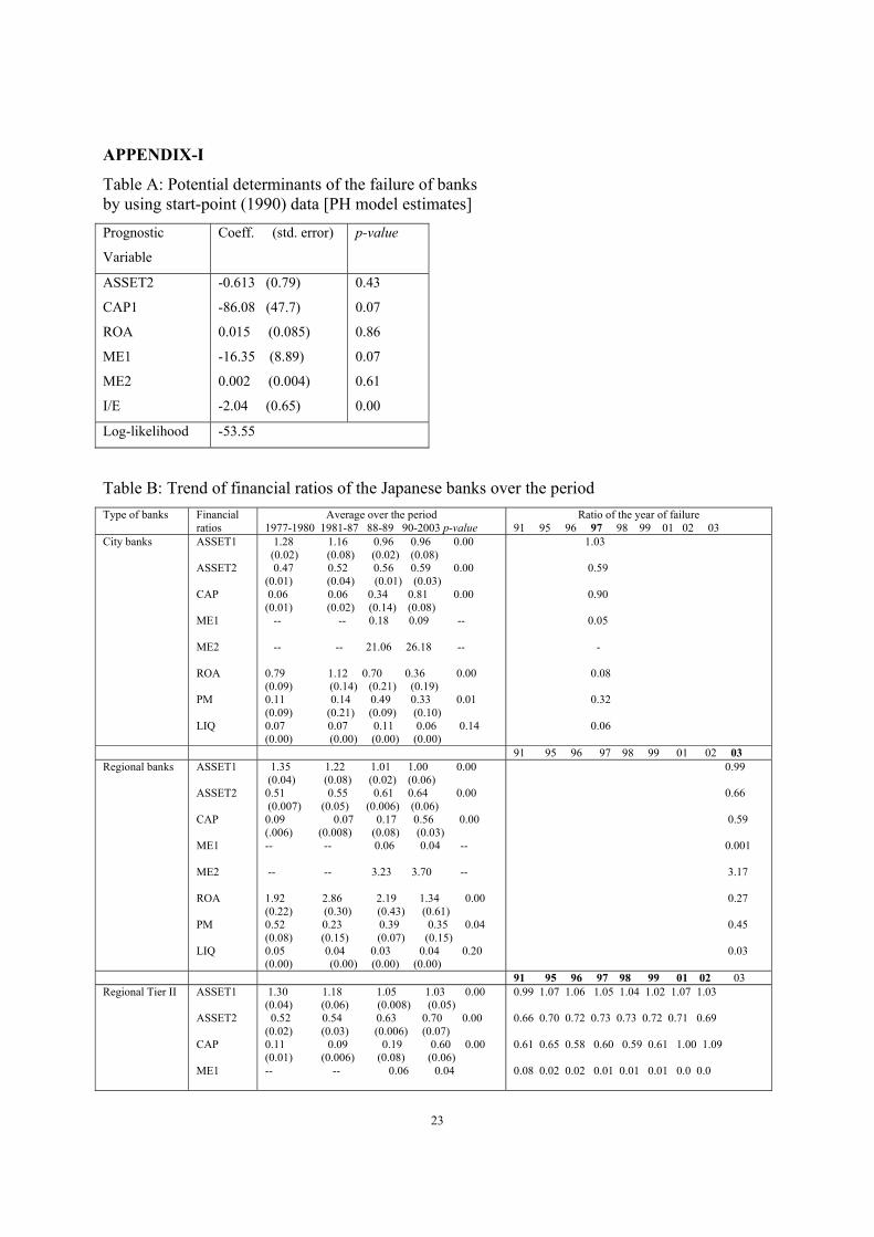
APPENDIX-I
Table A: Potential determinants of the failure of banks
by using start-point (1990) data [PH model estimates]
Prognostic
Variable
Coeff. (std. error) p-value
ASSET2
CAP1
ROA
ME1
ME2
I/E
-0.613 (0.79)
-86.08 (47.7)
0.015 (0.085)
-16.35 (8.89)
0.002 (0.004)
-2.04 (0.65)
0.43
0.07
0.86
0.07
0.61
0.00
Log-likelihood -53.55
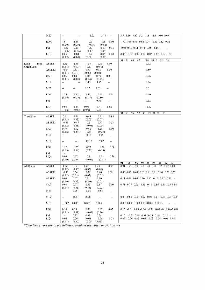
Table B: Trend of financial ratios of the Japanese banks over the period
Type of banks Financial
ratios
Average over the period
1977-1980 1981-87 88-89 90-2003 p-value
Ratio of the year of failure
91 95 96 97 98 99 01 02 03
City banks ASSET1
ASSET2
CAP
ME1
ME2
ROA
PM
LIQ
1.28 1.16 0.96 0.96 0.00
(0.02) (0.08) (0.02) (0.08)
0.47 0.52 0.56 0.59 0.00
(0.01) (0.04) (0.01) (0.03)
0.06 0.06 0.34 0.81 0.00
(0.01) (0.02) (0.14) (0.08)
-- -- 0.18 0.09 --
-- -- 21.06 26.18 --
0.79 1.12 0.70 0.36 0.00
(0.09) (0.14) (0.21) (0.19)
0.11 0.14 0.49 0.33 0.01
(0.09) (0.21) (0.09) (0.10)
0.07 0.07 0.11 0.06 0.14
(0.00) (0.00) (0.00) (0.00)
1.03
0.59
0.90
0.05
-
0.08
0.32
0.06
91 95 96 97 98 99 01 02 03
Regional banks ASSET1
ASSET2
CAP
ME1
ME2
ROA
PM
LIQ
1.35 1.22 1.01 1.00 0.00
(0.04) (0.08) (0.02) (0.06)
0.51 0.55 0.61 0.64 0.00
(0.007) (0.05) (0.006) (0.06)
0.09 0.07 0.17 0.56 0.00
(.006) (0.008) (0.08) (0.03)
-- -- 0.06 0.04 --
-- -- 3.23 3.70 --
1.92 2.86 2.19 1.34 0.00
(0.22) (0.30) (0.43) (0.61)
0.52 0.23 0.39 0.35 0.04
(0.08) (0.15) (0.07) (0.15)
0.05 0.04 0.03 0.04 0.20
(0.00) (0.00) (0.00) (0.00)
0.99
0.66
0.59
0.001
3.17
0.27
0.45
0.03
91 95 96 97 98 99 01 02 03
Regional Tier II ASSET1
ASSET2
CAP
ME1
1.30 1.18 1.05 1.03 0.00
(0.04) (0.06) (0.008) (0.05)
0.52 0.54 0.63 0.70 0.00
(0.02) (0.03) (0.006) (0.07)
0.11 0.09 0.19 0.60 0.00
(0.01) (0.006) (0.08) (0.06)
-- -- 0.06 0.04
0.99 1.07 1.06 1.05 1.04 1.02 1.07 1.03
0.66 0.70 0.72 0.73 0.73 0.72 0.71 0.69
0.61 0.65 0.58 0.60 0.59 0.61 1.00 1.09
0.08 0.02 0.02 0.01 0.01 0.01 0.0 0.0
24
ME2
ROA
PM
LIQ
-- -- 3.23 3.70 --
1.61 2.43 2.0 1.24 0.00
(0.20) (0.27) (0.38) (0.62)
0.30 0.21 0.43 0.33 0.35
(0.07) (0.16) (0.03) (0.19)
0.05 0.04 0.04 0.02 0.00
(0.02) (0.00) (0.00) (0.00)
3.5 3.50 3.40 5.2 4.8 4.8 10.0 10.9
1.79 1.05 0.96 0.62 0.44 0.40 0.42 0.31
-0.03 0.52 0.51 0.44 0.40 0.48 - -
0.03 0.02 0.02 0.02 0.02 0.02 0.02 0.04
91 95 96 97 98 99 01 02 03
Long Term
Credit Bank
ASSET1
ASSET2
CAP
ME1
ME2
ROA
PM
LIQ
1.35 2.06 1.59 0.90 0.00
(0.06) (0.37) (0.17) (0.80)
0.64 0.63 0.63 0.59 0.00
(0.01) (0.01) (0.00) (0.03)
0.06 0.04 0.48 0.79 0.00
(0.01) (0.01) (0.24) (0.22)
-- -- 0.13 0.05 --
-- -- 12.7 9.02 --
1.35 2.06 1.59 0.90 0.01
(0.06) (0.37) (0.17) (0.80)
-- -- -- 0.33 --
0.03 0.03 0.05 0.4 0.82
(0.00) (0.00) (0.00) (0.01)
0.92
0.59
0.96
0.04
6.5
0.60
0.32
0.02
91 95 96 97 98 99 01 02 03
Trust Bank ASSET1
ASSET2
CAP
ME1
ME2
ROA
PM
LIQ
0.45 0.44 0.43 0.44 0.98
(0.02) (0.03) (0.03) (0.07)
0.45 0.47 0.51 0.47 0.53
(0.02) (0.05) (0.03) (0.05)
0.19 0.12 0.60 1.29 0.00
(0.02) (0.04) (0.31) (0.29)
-- -- 0.13 0.05 --
-- -- 12.17 9.02 --
1.12 1.25 0.77 0.38 0.00
(0.19) (0.04) (0.31) (0.38)
--
0.06 0.07 0.11 0.08 0.50
(0.00) (0.00) (0.01) (0.01)
91 95 96 97 98 99 01 02 03
All Banks ASSET1
ASSET2
ASSET3
CAP
ME1
ME2
ME3
ROA
PM
LIQ
1.26 1.16 0.97 1.23 0.35
(0.02) (0.03) (0.03) (0.07)
0.50 0.54 0.58 0.60 0.00
(0.02) (0.05) (0.03) (0.05)
0.06 0.07 0.11 0.10
(0.00) (0.02) (0.00) (0.01)
0.08 0.07 0.33 0.87 0.00
(0.01) (0.01) (0.14) (0.22)
-- 0.08 0.08 0.03 --
-- 26.8 20.47 -- --
0.002 0.003 0.005 0.004
0.10 0.23 0.30 0.09 0.65
(0.01) (0.01) (0.01) (0.10)
-- 0.23 0.39 0.34
0.06 0.06 0.08 0.06 0.28
(0.01) (0.00) (0.00) (0.01)
0.91 1.55 1.50 1.47 1.41 1.37 1.32 1.02 1.00
0.56 0.63 0.63 0.62 0.61 0.61 0.60 0.59 0.57
0.11 0.09 0.09 0.10 0.10 0.10 0.12 0.11 -
0.71 0.77 0.75 0.81 0.81 0.86 1.31 1.15 0.98
0.08 0.03 0.02 0.02 0.01 0.01 0.01 0.01 0.00
0.002 0.003 0.003 0.003 0.004 0.003 - - -
0.15 -0.31 0.00 -0.54 -0.38 0.09 -0.56 0.65 0.8
0.15 -0.51 0.40 0.38 0.39 0.49 0.45 - -
0.09 0.06 0.05 0.05 0.03 0.04 0.04 0.04 -
*Standard errors are in parentheses; p-values are based on F-statistics
25
Figure 2: Plot of hazard functions (Kaplan-Meier’s estimate)
Hazard Function
Failure time in year from 1977
3020100
Cum
Hazard
2.5
2.0
1.5
1.0
.5
0.0
-.5
ASSET1
>=1.0
censored
<1.0
censored
Hazard Function
Failure time in year from 1977
3020100-10
Cu
m H
az
ard
2.5
2.0
1.5
1.0
.5
0.0
-.5
ASSET2
>=0.55
censored
<0.55
censored
Hazard Function
Failure time in year from 1977
3020100
Cum
Hazard
2.0
1.5
1.0
.5
0.0
-.5
ROA
>0.1
censored
<0.10
censored
Hazard Function
Failure time in year from 1977
3020100
Cu
m H
az
ard
2.5
2.0
1.5
1.0
.5
0.0
-.5
ASSET3
>=0.10
censored
<0.10
censored
Hazard Function
Failure time in year from 1977
3020100
Cu
m H
az
ard
2.0
1.5
1.0
.5
0.0
-.5
CAP
>=0.8
censored
<0.8
censored
Hazard Function
Failure time in year from 1977
3020100
Cu
m H
az
ard
2.5
2.0
1.5
1.0
.5
0.0
-.5
ME1
>=0.10
censored
<0.10
censored
Hazard Function
Failure time in year from 1977
3020100
Cu
m H
az
ard
2.0
1.5
1.0
.5
0.0
-.5
ME2
>=30
censored
<30
censored
Hazard Function
Failure time in year from 1977
3020100
Cum
Hazard
2.0
1.5
1.0
.5
0.0
-.5
PM
>0.30
censored
<=0.30
censored
Hazard Function
Failure time in year from 1977
3020100
Cum
Hazard
2.5
2.0
1.5
1.0
.5
0.0
-.5
LIQ
>0.06
censored
<=0.06
censored
26
Figure 3: Testing the proportionality of the hazard functions
Log Surv iv al Function
Year of survival from 1977
3020100
Log S
urv
ival
.5
0.0
-.5
-1.0
-1.5
-2.0
ROA1
>=0.10
2-censored
<0.10
1-censored
Log Survival Function
Year of survival from 1977
3020100
Lo
g S
urv
iva
l
.5
0.0
-.5
-1.0
-1.5
-2.0
-2.5
ASSET11
>=0.10
2-censored
<0.10
1-censored
Log Survival Function
Year of survival from 1977
3020100
Log S
urv
ival
.5
0.0
-.5
-1.0
-1.5
-2.0
ASSET33
>=0.10
2-censored
<0.10
1-censored
Log Surv iv al Function
Year of survival from 1977
3020100-10
Lo
g S
urv
iva
l.5
0.0
-.5
-1.0
-1.5
-2.0
-2.5
ASSET22
>=0.55
2-censored
<0.55
1-censored
Log Surv iv al Function
Year of survival from 1977
3020100
Lo
g S
urv
iva
l
.5
0.0
-.5
-1.0
-1.5
-2.0
CAP11
>=0.80
2-censored
<0.80
1-censored
Log Survival Function
Year of survival from 1977
3020100
Log S
urv
ival
.5
0.0
-.5
-1.0
-1.5
-2.0
ME22
>=30
2-censored
<30
1-censored
27
Figure-4: Different indicators of the Japanese economy during 1964-2003
Growth of Money supply and Base money
.00
5.00
10.00
15.00
20.00
25.00
30.00
1964 1967 1970 1973 1976 1979 1982 1985 1988 1991 1994 1997
M2+CD HPM
Call rate and Discount rate
.00
2.00
4.00
6.00
8.00
10.00
12.00
14.00
1964 1967 1970 1973 1976 1979 1982 1985 1988 1991 1994 1997
CR DISC
Growth of GDP and GNP
-5.00
.00
5.00
10.00
15.00
20.00
25.00
1964 1967 1970 1973 1976 1979 1982 1985 1988 1991 1994 1997
GNP GDP
Stock price index (Left) and Land Price index
.00
5000.00
10000.00
15000.00
20000.00
25000.00
30000.00
35000.00
40000.00
1964 1967 1970 1973 1976 1979 1982 1985 1988 1991 1994 1997
.00
20.00
40.00
60.00
80.00
100.00
120.00
NIKK225 LPI
Growth of WPI and CPI
-10
-5
0
5
10
15
20
25
1964 1967 1970 1973 1976 1979 1982 1985 1988 1991 1994 1997
WPI CPI
Growth of banks outstanding total loan and real
estate loan
0
1
2
3
4
5
6
7
8
1977 1981 1985 1989 1993 1997 2001
Real Estate Loan Total loan
28
APPENDIX-II
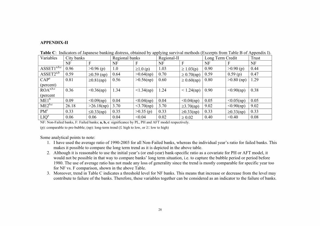
Table C: Indicators of Japanese banking distress, obtained by applying survival methods (Excerpts from Table B of Appendix I).
City banks Regional banks Regional-II Long Term Credit Trust Variables
NF F NF F NF F NF F NF
ASSET1a,b,c
0.96 >0.96 (p) 1.0 ≥1.0 (p) 1.03 ≥ 1.03(p) 0.90 >0.90 (p) 0.44
ASSET2a,b
0.59 ≥0.59 (np) 0.64 >0.64(np) 0.70 ≥ 0.70(np) 0.59 0.59 (p) 0.47
CAPa
(percent)
0.81 ≥0.81(np) 0.56 >0.56(np) 0.60 ≥ 0.60(np) 0.80 >0.80 (np) 1.29
ROAa,b,c
(percent
0.36 <0.36(np) 1.34 <1.34(np) 1.24 < 1.24(np) 0.90 <0.90(np) 0.38
ME1b
0.09 <0.09(np) 0.04 <0.04(np) 0.04 <0.04(np) 0.05 <0.05(np) 0.05
ME2b,c
26.18 >26.18(np) 3.70 <3.70(np) 3.70 ≥3.70(np) 9.02 <0.90(np) 9.02
PMc
0.33 ≤0.33(np) 0.35 >0.35 (p) 0.33 ≥0.33(np) 0.33 ≥0.33(np) 0.33
LIQa
0.06 0.06 0.04 <0.04 0.02 ≥ 0.02 0.40 <0.40 0.08 NF: Non-Failed banks, F: Failed banks; a, b, c: significance by PL, PH and AFT model respectively.
(p): comparable to pre-bubble; (np): long-term trend (≤ high to low, or ≥: low to high)
Some analytical points to note:
1. I have used the average ratio of 1990-2003 for all Non-Failed banks, whereas the individual year’s ratio for failed banks. This
makes it possible to compare the long term trend as it is depicted in the above table.
2. Although it is reasonable to use the initial year’s (or end-year) bank-specific ratio as a covariate for PH or AFT model, it
would not be possible in that way to compare banks’ long term situation, i.e. to capture the bubble period or period before
1980. The use of average ratio has not made any loss of generality since the trend is mostly comparable for specific year too
for NF vs. F comparison, shown in the above Table.
3. Moreover, trend in Table C indicates a threshold level for NF banks. This means that increase or decrease from the level may
contribute to failure of the banks. Therefore, these variables together can be considered as an indicator to the failure of banks.