the effect of the fluid film variable viscosity on the...

International Journal of Mechanical Engineering and Applications 2018; 6(1): 1-12

http://www.sciencepublishinggroup.com/j/ijmea

doi: 10.11648/j.ijmea.20180601.11

ISSN: 2330-023X (Print); ISSN: 2330-0248 (Online)

The Effect of the Fluid Film Variable Viscosity on the Hydrostatic Thrust Spherical Bearing Performance in the Presence of Centripetal Inertia and Surface Roughness

Ahmad Waguih Yacout Elescandarany

Department of Mechanical Engineering, Faculty of Engineering, Alexandria University, Alex, Egypt

Email address:

To cite this article: Ahmad Waguih Yacout Elescandarany. The Effect of the Fluid Film Variable Viscosity on the Hydrostatic Thrust Spherical Bearing

Performance in the Presence of Centripetal Inertia and Surface Roughness. International Journal of Mechanical Engineering and

Applications. Vol. 6, No. 1, 2018, pp. 1-12. doi: 10.11648/j.ijmea.20180601.11

Received: January 9, 2018; Accepted: January 22, 2018; Published: March 7, 2018

Abstract: In response to the importance of the industry great need to the hydrostatic thrust spherical bearing, this study is

performed. The stochastic modified Reynolds equation (developed by the author in his previous papers) applied to this type of

bearings has become more developed to deal with the bearing static performance under the effect of the fluid film viscosity

variation. The study showed the effect of the viscosity variation on the pressure, the load, the flow rate, the frictional torque,

the friction factor, the power factor, the stiffness factor and the central pressure ratio as well as the effect of the speed

parameter and the eccentricity on the temperature rise. The partial differential equation of the temperature gradient is derived

from the fluid governing equations, integrated and applied to this type of bearings to calculate and predict the temperature

distribution along the fluid film. The application of this temperature equation proved the excellence of the aforementioned

optimum design of this bearing in our previous papers where the temperature of the outlet flow was less than 14 degrees

centigrade over its inlet temperature.

Keywords: Hydrostatic Bearings, Spherical Bearings, Surface Roughness, Inertia Effect, Variable Viscosity Effect,

Temperature Rise of the Fluid Film

1. Introduction

Expanding the author’s previous studies on the hydrostatic

thrust spherical bearing, the viscosity variation has been

considered in re-developing the stochastic modified Reynolds

equation “modified by Dowson and stochastically developed

by the author” [1] to be thermally valid to deal with such type

of bearings.

Dowson and Taylor [2, 3] stated that running the bearing at

high speeds considerable temperature variation along the film

in (Ɵ) direction was observed, where it caused viscosity

variation affecting the bearing performance.

Essam Salem and Farid Khalil [4, 5] adopted a simple

form of the viscosity variation expression where it has been

introduced in the pressure gradient equation and numerically

solved to get the pressure and the temperature distribution. It

is found that temperature rise reduces the load and the

frictional torque while increases the flow rate.

Rowe and Stout [6] studied the design and the

manufacturing of the hydrostatic spherical bearing. It is

stated that the most critical situations encountered involve

high speeds and high flow rates when a reasonable estimate

of the temperature rise is obtained by assuming that all the

heat is carried out in the oil whereas the in slow moving

calculations this method tends to overestimate temperature

rise.

Keith Brockwell et al [7] studied the temperature

characteristics of a (PSJ) pivoted shoe journal bearing where

it is stated that the temperature with (load between pad)

reaches 100 C at 5000 rpm and a load of 22.24 KN and for

the same maximum temperature and load configuration the

offset pivot extends the bearing speed to be just under 6500

rpm. Generally it was found that differences between offset

and center pivot bearing temperature (both maximum and

75% pad locations) increased with speed and load.

Minhui He et al [8] stated that the fluid film journal

bearing is critical to machine’s overall reliability level and

concluded that the viscosity shearing generates heat in the

fluid film which lead to reduce the viscosity and to increase

the temperature and the power losses.

Srinivasan V. [9] studied the annular recess conical bearing

considering the inertia and the viscosity variation concluding

that the speed increase leads to raise the temperature and

pressure.

2 Ahmad Waguih Yacout Elescandarany: The Effect of the Fluid Film Variable Viscosity on the Hydrostatic Thrust Spherical Bearing Performance in the Presence of Centripetal Inertia and Surface Roughness

Shigang Wang et al [10] studied the temperature effect on

the hydrostatic bearing performance in both cases of

sufficient and deficient fluid film using the “Fluent 6.5

Software” to simulate the temperature field. According to the

obtained results, it is concluded that the oil will affect the

temperature distribution and the temperature rise.

Xibing Li et al [11] stated that during working the

viscosity changes as the temperature increases then the

bearing performance will be affected; therefore control

thermal deformation hydrostatic bearing and high efficiency

cooling is the prime problem to solve.

The present study could be considered as an extension to

the study of reference [1] whereas the lubricant viscosity has

been treated as a constant in turn it couldn’t be possible to

find out the bearing thermal behavior in general and to check

thermally the design of such pattern of bearing presented in

this reference.

This research has opened the door widely to study the

behavior of this type of bearings under the lubricant variable

viscosity in the presence of the centripetal inertia and the

surface roughness. The un- recessed fitted type of bearings

with its different configurations has been handled in this

paper.

Nomenclature

A = )6(3

ipeq πµ−

a =Bearing projected area (2

Rπ ).

C = )6( πµ qi− .

vc = Lubricant specific heat

iod =Bearing inlet orifice diameter.

E (f) =Expected value of.

e = Eccentricity.

f = Dimensionless friction factor.

F = Friction factor.

H = Dimensionless film thickness.

h = Film thickness.

oh = Deterministic part of the film thickness ( θcose ).

sth = Random stochastic part of the film thickness.

fh = Power factor

vK = Constant of viscosity variation

eK = ( Re ).

M = Dimensionless frictional torque ( 42 Remo Ωπµ ).

m = Frictional torque.

om = Deterministic part of the frictional torque.

stm = Random stochastic part of the frictional torque.

N = Shaft speed (rpm).

P = Dimensionless pressure (ipp ).

p = Mean pressure along the film thickness.

ip = Inlet pressure.

sp =Supply pressure ( 25105 mNx ).

Q = Dimensionless volume flow rate ( AQ −= ).

q = Flow volume flow rate

R = Bearing radius (50 mm).

S = Speed parameter (

ip

R22

40

3 Ωρ).

SF = Stiffness factor

T = Temperature u, v, w = Velocity components in the

r, θ , ϕ directions.

W = Dimensionless load carrying capacity (ipRw 2π ).

w = Load carrying capacity.

z = )( Rr −

β = (si pp ).

θ = Angle co-ordinate.

bφ = Seat outer rim angle.

iθ =Inlet flow angle.

eθ = Outlet flow angle.

ρ = Lubricant density ( 42.867 msN ).

σ = Dimensionless surface roughness parameter. 2

oσ = Variance of the film thickness.

λ = Bearing stiffness.

µ =Lubricant viscosity ( 2.068.0 msN )

Ω =Rotational speed.

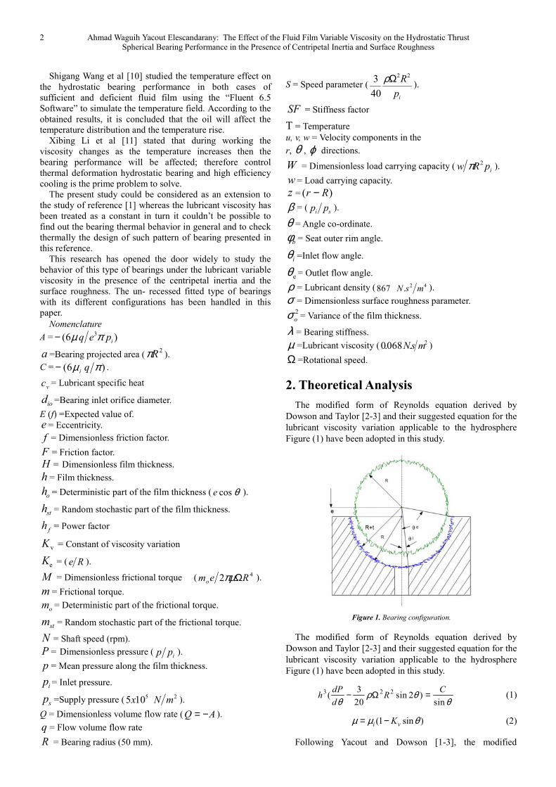
2. Theoretical Analysis

The modified form of Reynolds equation derived by

Dowson and Taylor [2-3] and their suggested equation for the

lubricant viscosity variation applicable to the hydrosphere

Figure (1) have been adopted in this study.

Figure 1. Bearing configuration.

The modified form of Reynolds equation derived by

Dowson and Taylor [2-3] and their suggested equation for the

lubricant viscosity variation applicable to the hydrosphere

Figure (1) have been adopted in this study.

3 2 23( sin 2 )

20 sin− Ω =dP C

h Rd

ρ θθ θ

(1)

(1 sin )= −i vKµ µ θ (2)

Following Yacout and Dowson [1-3], the modified

International Journal of Mechanical Engineering and Applications 2018; 6(1): 1-12 3

Reynolds equation becomes:

3 2 2 (1 sin )3[ sin 2 ]

20 sin

−− Ω = vC Kdph R

d

θρ θθ θ

(3)

Taking the expectation for both sides:

3 2 2 2 (1 sin )3( 3 )[ sin2 ]

20 sin

−+ − Ω = vo o o

C Kdph h R

d

θσ ρ θθ θ

(4)

2 2

3 2

(1 sin ) 3sin 2

20( 3 ) sin

−= + Ω+

v

o o o

C kdpR

d h h

θ ρ θθ σ θ

(5)

Putting the following dimensionless group and rearranging

give:

iP p p= ; oH h e cos= = θ ; o eσ = σ , 3iA C e P= ,

2 2S (3 40) R= ρ Ω , 2 23 bσ = , d (1 sin ) dHθ = − θ ,

iC 6 Q= − µ π

3 2 2

v1

3 2 2 2

AP dH 4S HdH

(H b H)(1 H )Ak

dH

(H b H)(1 H )

−= −+ −

+

+ −

∫ ∫

∫ (6)

3. Theoretical Solutions

3.1. Pressure Distribution

The integration of the 1st two parts of the pressure equation

(6) could be found in Yacout [1] as:

2 2 2

2 2

1 ln(1 sec ) ln(tan( ) 2 cos

1 2+ + − +

+A

b S Bb b

θ θ θ (7)

And the integration of the 3rd part of the equation could be

found in the appendix (A1) as:

2

2 2 2

1 1 sin 1 1 sin[ln ln ]

1 sin2 1 1 sin

+ + −= − +− + + +

bIntg

b b b

θ θθ θ

(8)

Restoring the 1st form again:

2 2

2 2

22

2 2 2

1 ln(1 sec ) ln(tan( ).....

1 2

1 sin 1 1 sinln( ) ln( ) 2 cos

1 sin2 1 1 sin

= + ++

+ + −− + − +− + + +

v

AP b

b b

k A bS B

b b b

θ θ

θ θ θθ θ

(9)

Applying the boundary conditions:

At = iθ θ → 1=P

At = eθ θ → 0=P

2 2

2 2

2 2 2 2

2

2 2

2 2 2

1 2 (cos cos )

1 sec tan1 1 ln( ) ln( .....

tan1 2 1 sec

1 sin 1 sinln( * ).......

1 sin 1 sin2

1 sin 1 sin1ln( * )

1 1 sin 1 sin

+ −=+ +

+ ++ −−− +

+ − + +++ + + + −

i e

i i

eo

v i o

i o

i e

i e

SA

b

b b b

k

b

b b

b b b

θ θθ θ

θθθ θθ θ

θ θθ θ

2

2 2

2 2

2

2 2 2

2 cos .....

1 ln(1 sec ) ln(tan( ).....

1 2

1 sin 1 sin1ln( ) ln( )

1 sin2 1 1 sin

=

− + ++

+ + −+ +− + + +

e

e e

v e e

e e

B S

Ab

b b

k A b

b b b

θ

θ θ

θ θθ θ

3.2. Load Carrying Capacity

Following Yacout and Dowson [1-3]:

e

i

e

i

e

i

2 2 2i i

2

2i

2

2

w R sin p 2 R p sin cos d

wW sin 2 P sin cos d

R p

W sin 2 P sin cos d

W sin 2F

θ

θθ

θθ

θ

= π θ + π θ θ θ

= = θ + θ θ θπ

= θ + θ θ θ

= θ +

∫

∫

∫

(10)

e

i

e

i

e

i

2 2

2 2

2 v

2

2

2 2

1 2

F Psin cos d

A 1[ ln(1 b sec ) ln(tan( )b 1 2b

k A 1 sin2Scos B]sin cos d ln( )

1 sin2b

1 b 1 sinln( )sin cos d

b 1 b 1 sina a

θ

θθ

θθ

θ

= θ θ θ

+ θ + θ+

+ θ− θ + θ θ θ −− θ

+ − θ+ θ θ θ+ + + θ

= −

∫

∫

∫

Where:

2 21 2 2

2

2 2

2

2 2

1[ ln(1 sec ) ln(tan( )

1 2

2 cos ]sin cos

1 sinln( )

1 sin2

1 1 sinln( )sin cos

1 1 sin

= + ++

− +

+=−

+ −++ + +

∫

∫

e

i

e

i

v

Aa b

b b

S B d

k Aa

b

bd

b b

θ

θ

θ

θ

θ θ

θ θ θ θ

θθ

θ θ θ θθ

The Integration of (a1) could be found in Yacout [1] as:

2 22 2

1 2 2

2 24

2 2

2

cos[ ln ( cos )4 ( 1)

sin cosln (sin ) ln (cos )] [cos ]

22( 1) 2

[cos ]

+= ++

− − ++

−

i e

e i

e

i

ba A b

b b

S

b b

B

θ θθ θ

θθ

θ θ

θ θθ θ θ

θ

And the integration of (a2) in Appendix (A2) as:

e

i

2 2 2 22 v

2 2 2

k A (cos ) (1 sin ) b cos ( b 1 sin )a [ ln ( )ln ]

2 (1 sin )4b 2 b 1 ( b 1 sin )

θθ

θ − θ + θ + − θ= −+ θ + + + θ


Then:

2

1 2

W sin 2FF a a

= θ += −

3.3. Temperature Distribution

From the appendix (A3):

22

i

v

2 4 2v

dP dP (S sin 2 )( ) 4S( ) sin(2 )

dT p d d 0.21( )dPd c

(2 sin 2 )d

(Const) sin sec (1 k sin )X

dP(2 sin 2 )

d

θ− θ +θ θ=

θ ρ θ −θ

θ θ − θ+ =θ −

θ

n n 1

1 i2i

2 4i e

i

TX

T T XT T

160SConst ( )

p R K(1 K sin )

−

∆ =∆θ

= + ∆θ=

µ=ρ

µ = µ − θ

(11)

3.4. Frictional Torque

Following Yacout and Dowson [1-3]:

4 32 sinΩ= =∫ ∫e e

i i

Rm dm d

e h

θ θ

θ θ

π µ θ θ (12)

(1 sin )= −i vkµ µ θ

3

4

(1 sin )sin

2

−=Ω ∫

e

i

v

i

kmed

hR

θ

θ

θ θ θπ µ

3(1 sin )sin−= ∫

e

i

vkM d

h

θ

θ

θ θ θ

3(1 sin )sin−= ∫

e

i

vkM d

h

θ

θ

θ θ θ

2 2 2 2

3 3

1 cos( )

cos

+ += =hE

h h

σ θ σθ

Taking the expectation of both sides:

2 2 3

3

(cos )(1 sin )sin

cos

+ −= ∫e

i

vkM d

θ

θ

θ σ θ θ θθ

2 2 2

3

(cos )(1 sin )sin(cos )

cos

+ −= −∫e

i

vkM d

θ

θ

θ σ θ θ θθ

2 2 2

3

(cos )(1 sin )(1 cos )(cos )

cos

+ − −= −∫e

i

vkM d

θ

θ

θ σ θ θ θθ

2 2 2

3

(cos )(1 sin )(cos 1)(cos )

cos

+ − −= ∫e

i

vkM d

θ

θ

θ σ θ θ θθ

The Integration could be found in the Appendix (A4) as:

2 22

2

2

2 3

cos[ ( 1) ln (cos ) ]

2 2cos

[( 1)sin ln (tan sec )

sinln (sec tan ) sec tan ]

2 3

= + − + − −

− − + −

+ − −

e

i

e

i

v

M

k

θθ

θθ

θ σσ θθ

σ θ θ θ

σ θθ θ θ θ

(13)

3.5. Volume Flow Rate

From Yacout [1]:

= −Q A (14)

3.6. Friction Factor

From Yacout [1]:

=F M W (15)

3.7. Power Factor

From Yacout [1]:

2 3cos=f

e

Qh

W

πθ

(16)

3.8. Stiffness Factor

From Yacout [1]:

_ _

( )= − +SF W Wβ β (17)

4. Results

Where the main objective of this study is to find out the

bearing thermal behavior under the lubricant viscosity

variation in the presence of the centripetal inertia and the

surface roughness, and because of the complexity of the

theoretical solution it was necessary to compare between

different forms of viscosity equations to adopt the one which

can help in facilitating the theoretical derivation of some

equations that represent the bearing characteristics. Deriving

such equations it was preferably applied to the un-recessed

fitted type of bearings to predict its behavior. The bearing

characteristics such as pressure distribution, temperature

distribution, load carrying capacity, flow rate, frictional

torque, friction factor and stiffness factor have been

calculated for the bearing with hemispherical and partially

hemispherical seats. Figures (2-13) represent the bearing with

hemispherical and partially hemispherical seats respectively.

5. Discussion

It is found to be necessary to study the bearing thermal

behavior since it hasn’t been accomplished in Yacout [1]. The

visions of Dowson [2, 3] and Essam and Farid [4, 5] of the


lubricant viscosity and temperature gradient for the

hydrostatic spherical bearing respectively have been adopted.

The example of the designed bearing offered in Yacout [1]

has been used as a guide in the research.

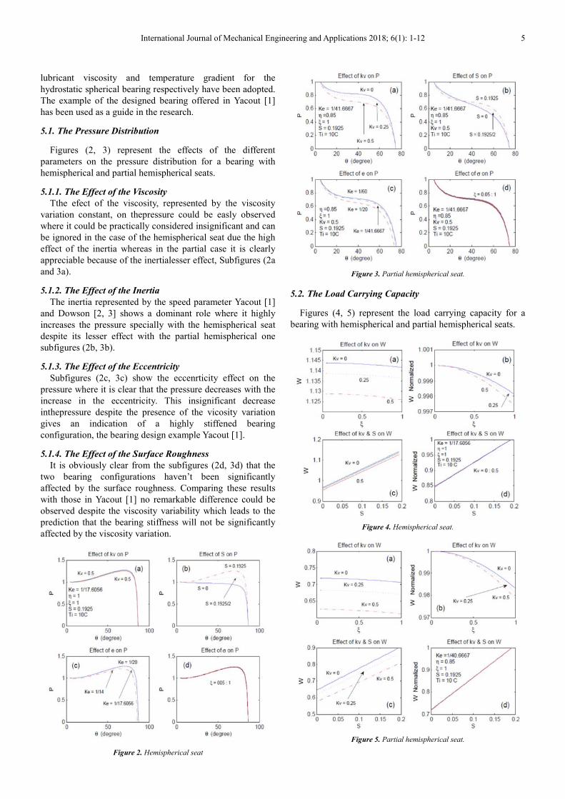
5.1. The Pressure Distribution

Figures (2, 3) represent the effects of the different

parameters on the pressure distribution for a bearing with

hemispherical and partial hemispherical seats.

5.1.1. The Effect of the Viscosity

Tthe efect of the viscosity, represented by the viscosity

variation constant, on thepressure could be easly observed

where it could be practically considered insignificant and can

be ignored in the case of the hemispherical seat due the high

effect of the inertia whereas in the partial case it is clearly

appreciable because of the inertialesser effect, Subfigures (2a

and 3a).

5.1.2. The Effect of the Inertia

The inertia represented by the speed parameter Yacout [1]

and Dowson [2, 3] shows a dominant role where it highly

increases the pressure specially with the hemispherical seat

despite its lesser effect with the partial hemispherical one

subfigures (2b, 3b).

5.1.3. The Effect of the Eccentricity

Subfigures (2c, 3c) show the eccenrticity effect on the

pressure where it is clear that the pressure decreases with the

increase in the eccentricity. This insignificant decrease

inthepressure despite the presence of the vicosity variation

gives an indication of a highly stiffened bearing

configuration, the bearing design example Yacout [1].

5.1.4. The Effect of the Surface Roughness

It is obviously clear from the subfigures (2d, 3d) that the

two bearing configurations haven’t been significantly

affected by the surface roughness. Comparing these results

with those in Yacout [1] no remarkable difference could be

observed despite the viscosity variability which leads to the

prediction that the bearing stiffness will not be significantly

affected by the viscosity variation.

Figure 2. Hemispherical seat

Figure 3. Partial hemispherical seat.

5.2. The Load Carrying Capacity

Figures (4, 5) represent the load carrying capacity for a

bearing with hemispherical and partial hemispherical seats.

Figure 4. Hemispherical seat.



5.2.1. The Effect of the Viscosity

Subfigures (4a, 5a) show the load decrease with the

increase in both of the viscosity variation costant and the

surface roughness. Normalizing the load, Subfigures (4b, 5b)

show that the decrease in the load- due to the viscosity

variation constant increase- is increasing as the surface

roughness increases, i.e, at a point with certain value of the

surface roughness parameter the decrease in the load due to

the viscosity variation will increase at another point with

higher value. And the relatively whole loss in the load along

the surface parameter scale will increase as the vicosity

variation constant increases.

5.2.2 The Effect of the Inertia

As seen from subfigures (4c, 5c), the load is positively

affected by the inertia and negatively by the viscosity

variation. It is also clear that the load decrease due to the

viscosity variation in the case of hemispherical seat is less

than that of the partial hemisperical one because of the more

effective role of the inertia as said before in the pressure.

Normalizing the load subfigures (4d, 5d), show that the load

decrease due to the viscosity variation is not affected by the

increase in the inertia (speed parameter) and the relatively net

gain in the load due to the inertia will not be affected by the

viscosity variation.

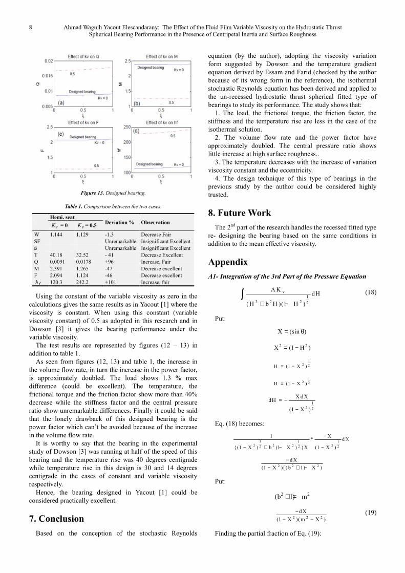
5.3. The Volume Flow Rate, the Frictional Factor, the

Friction Factor and the Power Factor

Figures (6, 7) represent the volume flow rate, the frictional

torque, the friction factor and the power factor for the same

bearing with the hemispherical and the partial hemispherical

seats.

It could be seen from the two figures that the volume flow

rate and the power factor increase with the increase in the

viscosity variation constant, subfigures (6a, d) and subfigures

(7a, d) while the frictional torque and the friction factor

decrease subfigures (6b, c) and subfigures

(7b, c). It looks reasonable and logical because of the

viscosity decrease.



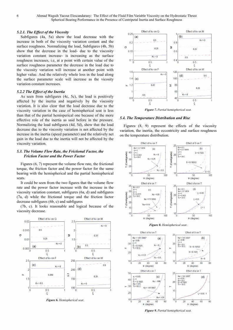
5.4. The Temperature Distribution and Rise

Figures (8, 9) represent the effects of the viscosity

variation, the inertia, the eccentricity and surface roughness

on the temperature distribution.




It is clear that the temperature decreases with the viscosity

variation constant increase, subfigures (8a, 9a).

5.4.1. The Effect of the Viscosity Variation Constant

It is clear that the temperature decreases with the viscosity

variation constant increase, subfigures (8a, 9a).

5.4.2. The Effect of the Inertia

Subfigures (8b, 9b) shows that the inertia plays an

important role in raising the temperature.

5.4.3. The Effect of the Eccentricity

Subfigures (8c, 9c) shows that the temperature is

positively affected with decrease in the eccentricity.

5.4.4. The effect Of the Surface Roughness

Subfigures (8d, 9d) shows that the surface roughness has

the least effect on the temperature where it could be

practiclly ignored.

Generally, it could be said that Just a look at the pressure

equation shows its complicated relation with the inertia, the

eccentricity, the surface roughness and the viscosity; and

another look at the equation of the temperature gradient

shows its complicated relation with the pressure gradient, the

inertia and viscosity. The study of these complicated relations

controlling the temperature rise could facilitate the designer

job.

5.5. The Stiffness Factor and the Central Pressure Ratio

Figures (10, 11) represent the effects of the viscosity

variation constant on the stiffness factor and the central

pressure ratio.

5.5.1. The Stiffness Factor

The bearing with the hemispherical seat shows no

remarkable effect on the stiffness factor due to the vicosity

variation whereas the bearing with the partial hemispherical

seat shows decrease with the viscosity variation constant,

subfigures (10a, 11a). The normalization of the stiffness

factor shows that the bearing behavior hasn’t been affected

regardless the seat type i.e, the stiffness factor versus the

surface roughness has a fixed shape, subfigures (10b, 11b).


5.5.2. The Central Pressure Ratio

Subfigures (10c, 11c) show the effect of the central

pressure ratio with the viscosity variation. Despite the unsean

effect in the case of the hemispherical seat Subfigures (10d,

11d) reveal the the central pressure ratio increase with the

viscosity variation constant.


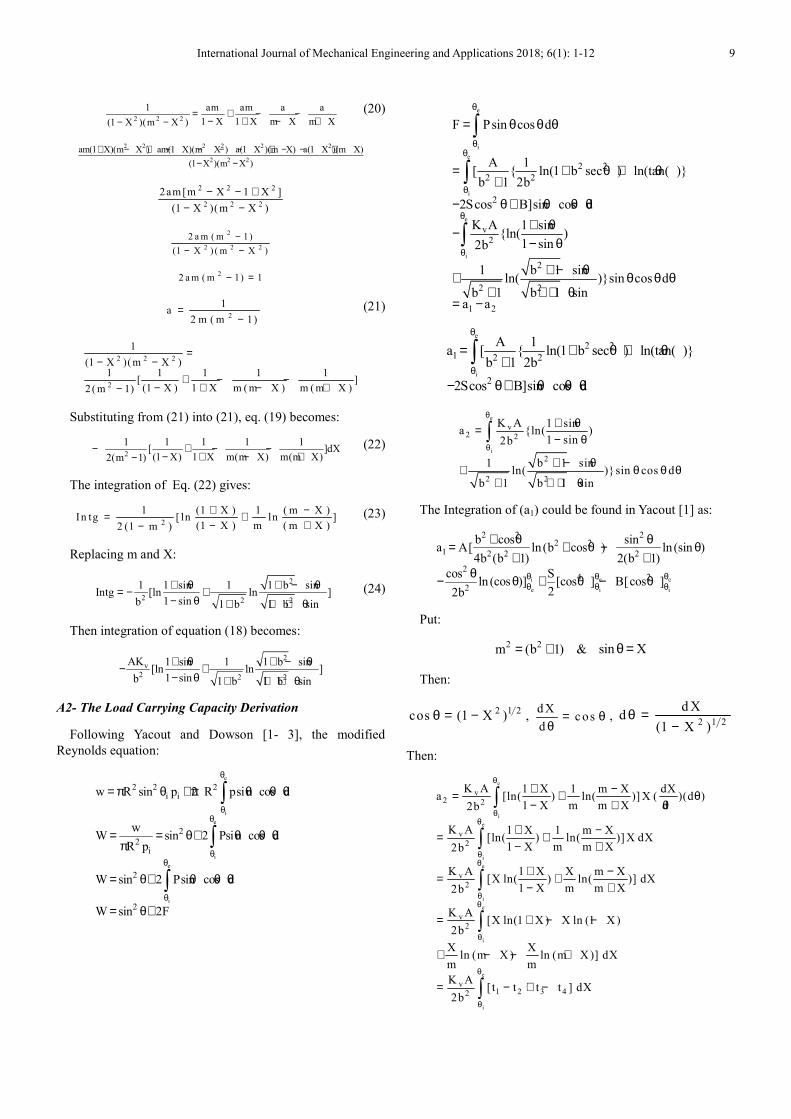
6. Testing the Designed Bearing

One of the objectives of this study is testing the bearing

designed by Yacout [1] showing the performance deviation

when considering the variable viscosity. The bearing has:

R 50 mm= , o

i 5φ = , 1.0η = , 0.05ξ = , N 100 rps= ,

N 100 rps= ,2 4867 N.s mρ = , 2 3β = ,

20.068 N.s mµ= ,

eK 1 17.6056= , vK 0= , vK 0.5=

Figure 12 designed bearing.


Figure 13. Designed bearing.

Table 1. Comparison between the two cases.

Hemi. seat

Deviation % Observation vK = 0 vK = 0.5

W 1.144 1.129 -1.3 Decrease Fair

SF Unremarkable Insignificant Excellent

ß Unremarkable Insignificant Excellent

T 40.18 32.52 - 41 Decrease Excellent

Q 0.0091 0.0178 +96 Increase, Fair

M 2.391 1.265 -47 Decrease excellent

F 2.094 1.124 -46 Decrease excellent

fh 120.3 242.2 +101 Increase, fair

Using the constant of the variable viscosity as zero in the

calculations gives the same results as in Yacout [1] where the

viscosity is constant. When using this constant (variable

viscosity constant) of 0.5 as adopted in this research and in

Dowson [3] it gives the bearing performance under the

variable viscosity.

The test results are represented by figures (12 – 13) in

addition to table 1.

As seen from figures (12, 13) and table 1, the increase in

the volume flow rate, in turn the increase in the power factor,

is approximately doubled. The load shows 1.3 % max

difference (could be excellent). The temperature, the

frictional torque and the friction factor show more than 40%

decrease while the stiffness factor and the central pressure

ratio show unremarkable differences. Finally it could be said

that the lonely drawback of this designed bearing is the

power factor which can’t be avoided because of the increase

in the volume flow rate.

It is worthy to say that the bearing in the experimental

study of Dowson [3] was running at half of the speed of this

bearing and the temperature rise was 40 degrees centigrade

while temperature rise in this design is 30 and 14 degrees

centigrade in the cases of constant and variable viscosity

respectively.

Hence, the bearing designed in Yacout [1] could be

considered practically excellent.

7. Conclusion

Based on the conception of the stochastic Reynolds

equation (by the author), adopting the viscosity variation

form suggested by Dowson and the temperature gradient

equation derived by Essam and Farid (checked by the author

because of its wrong form in the reference), the isothermal

stochastic Reynolds equation has been derived and applied to

the un-recessed hydrostatic thrust spherical fitted type of

bearings to study its performance. The study shows that:

1. The load, the frictional torque, the friction factor, the

stiffness and the temperature rise are less in the case of the

isothermal solution.

2. The volume flow rate and the power factor have

approximately doubled. The central pressure ratio shows

little increase at high surface roughness..

3. The temperature decreases with the increase of variation

viscosity constant and the eccentricity.

4. The design technique of this type of bearings in the

previous study by the author could be considered highly

trusted.

8. Future Work

The 2nd

part of the research handles the recessed fitted type

re- designing the bearing based on the same conditions in

addition to the mean effective viscosity.

Appendix

A1- Integration of the 3rd Part of the Pressure Equation

v1

3 2 2 2

A KdH

( H b H )(1 H )+ −∫ (18)

Put:

X (sin )= θ

2 2X (1 H )= −

12 2H (1 X )= −

12 2H (1 X )= −

1

2 2

X dXdH

(1 X )

= −

−

Eq. (18) becomes:

3 1 1

2 2 2 22 2 2

1 X* d X

(1 X ) b (1 X ) X (1 X )

−

− + − −

2 2 2

d X

(1 X )[ ( b 1) X )

−− + −

Put:

2 2(b 1) m+ =

2 2 2

d X

(1 X )( m X )

−− −

(19)

Finding the partial fraction of Eq. (19):


2 2 2

1 am am a a

1 X 1 X m X m X(1 X )(m X )= + − −

− + − +− − (20)

2 2 2 2 2 2

2 2 2

am(1 X)(m X ) am(1 X)(m X ) a(1 X )(m X) a(1 X )(m X)

(1 X )(m X )

+ − + − − − − + − − +− −

2 2 2

2 2 2

2am [m X 1 X ]

(1 X )( m X )

− − +− −

2

2 2 2

2 a m ( m 1)

(1 X ) ( m X )

−− −

22 a m ( m 1) 1− =

2

1a

2 m ( m 1)=

− (21)

2 2 2

2

1

(1 X )( m X )1 1 1 1 1

[ ](1 X ) 1 X m ( m X ) m ( m X )2( m 1)

=− −

+ − −− + − +−

Substituting from (21) into (21), eq. (19) becomes:

2

1 1 1 1 1[ ]dX(1 X) 1 X m(m X) m(m X)2(m 1)

− + − −− + − +−

(22)

The integration of Eq. (22) gives:

2

1 (1 X ) 1 ( m X )In tg [ ln ln ]

(1 X ) m ( m X )2 (1 m )

+ −= +− +−

(23)

Replacing m and X:

2

2 2 2

1 1 sin 1 1 b sinIntg [ln ln ]

1 sinb 1 b 1 b sin

+ θ + − θ= − +− θ + + + θ

(24)

Then integration of equation (18) becomes:

2v

2 2 2

AK 1 sin 1 1 b sin[ln ln ]

1 sinb 1 b 1 b sin

+ θ + − θ− +− θ + + + θ

A2- The Load Carrying Capacity Derivation

Following Yacout and Dowson [1- 3], the modified

Reynolds equation:

e

i

e

i

e

i

2 2 2i i

2

2i

2

2

w R sin p 2 R psi n cos d

wW sin 2 Psi n cos d

R p

W sin 2 Psin cos d

W sin 2F

θ

θθ

θθ

θ

= π θ + π θ θ θ

= = θ+ θ θ θπ

= θ+ θ θ θ

= θ+

∫

∫

∫

e

i

e

i

e

i

2 2

2 2

2

v2

2

2 2

1 2

F Psin cos d

A 1[ ln(1 b sec ) ln(tan( )b 1 2b

2Scos B]sin cos d

K A 1 sinln( )

1 sin2b


b 1 b 1 sina a

θ

θθ

θ

θ

θ

= θ θ θ

= + θ + θ+

− θ + θ θ θ+ θ−− θ

+ − θ+ θ θ θ+ + + θ

= −

∫

∫

∫

e

i

2 21 2 2

2

A 1a [ ln(1 b sec ) ln(tan( )

b 1 2b

2Scos B]sin cos d

θ

θ

= + θ + θ+

− θ+ θ θ θ

∫

e

i

v2 2

2

2 2

K A 1 sina ln( )

1 sin2b


b 1 b 1 sin

θ

θ

+ θ=− θ

+ − θ+ θ θ θ+ + + θ

∫

The Integration of (a1) could be found in Yacout [1] as:

e ei

e i i

2 2 22 2

1 2 2 2

24 2

2

b cos sina A[ ln (b cos ) ln (sin )

4b (b 1) 2(b 1)

cos Sln (cos )] [cos ] B[cos ]

22b

θ θθθ θ θ

+ θ θ= + θ − θ+ +

θ− θ + θ − θ

Put:

2 2m (b 1)= + & sin Xθ =

Then:

2 1 2cos (1 X )θ = − , d X

c osd

= θθ

, 2 1 2

d Xd

(1 X )θ =

−

Then:

e

i

e

i

e

i

e

i

v2 2

v2

v2

v2

v1 2 32

K A 1 X 1 m X dXa [ln( ) ln( )] X ( )(d )

1 X m m X d2b

K A 1 X 1 m X[ln( ) ln( )] X dX

1 X m m X2b

K A 1 X X m X[X ln( ) ln( )] dX

1 X m m X2b

K A[X ln(1 X) X ln (1 X)

2b

X Xln (m X ) ln (m X)] dX

m m

K A[t t t

2b

θ

θθ

θθ

θθ

θ

+ −= + θ− + θ

+ −= +− +

+ −= +− +

= + − −

+ − − +

= − + −

∫

∫

∫

∫

e

i

4t ] dX

θ

θ∫


1

2

3

4

t X ln(1 X)t X ln(1 X)

Xt ln(m X)

mX

t ln(m X)m

= += −

= −

= +

Integration of each term:

e e e

i i i

e

i

e e

i i

e e

i i

1

2

2

t dX X ln(1 X) dX X ln(1 X) dX

[(1 X) ln(1 X) ln(1 X)]d(1 X)

(1 X ) ln(1 X) d(1 X) ln(1 X)]d(1 X)

(1 X) 1[ ln (1 X) ] [(1 X)ln (1 X) 1]

2 2(X 1) (X 3)

[ ln (1 X) (1 X) ]2 4

θ θ θ

θ θ θθ

θθ θ

θ θ

θ θθ θ

θ

= + = +

= + + − + +

= + + + − + +

+= + − − + + −

− −= + − +

∫ ∫ ∫

∫

∫ ∫

e

i

θ

e

i

e

i

e

e

i

i

2

2

2

1

( X 1) 3 X[ln (1 X ) ]

2 2(1 X )

(1 X ) 3 X[ ln (1 X )]

2 2(1 X )T hen :

(1 X ) 3 Xt dX [ ln (1 X )]

2 2(1 X )

θθ

θθ

θθθ

θ

− −= + −−

− −= − +−

− −= − +−∫

Integration of (t2) could be done as (t1) with changing the

sign of (X) to be:

e

i

e

i

2

2

t dX X ln (1 X )dX

(1 X ) 3 X[ ln (1 X )]

2 2(1 X )

θ

θ

θθ

= −

− += − −+

∫

Integration of (t3)

e e

i i

e

i

e

i

e

i

e

i

3

2

X 1t dX ln(m X)dX Xln(m X)dX

m m

1[(m X)ln(m X) mln(m x) ]dX(m x)

m

1[(m X)ln(m X)]d(m X)

m

ln(m X) d(m X)

1 (m X) 1[ ln(m X) (m X)ln(m X) 1]m 2 2

Re arranging :

θ θ

θ θθ

θθ

θθ

θ

θθ

= − = −

= − − − − −

= − − −

− − −

−= − − − − − −−

∫ ∫

∫

∫

∫

e

i

e

e

i

i

2 2 2 2

2 2 2 2

3

m X 3m 2mX X[ ln(m X) ]

2m 4mThen :

X m X 2mX 3mt dX [ ln(m X) ]

2m 4m

θθ

θθθ

θ

− + − + += − −

− + −= − −∫

Integration of (t4):

It could be done as in (t3) or directly you get the

integration after changing the sign of (X) to be:

e

e

i

i

2 2 2 2

4

X m X 2mX 3mt dX [ ln(m X) ]

2m 4m

θθθ

θ

− − −= + −∫Simplifying:

e e

e

i

i i

2 2

3 4

m X (m X)t dX t dX [( ) ln X]

2m (m X)

θ θθθ

θ θ

− +− = −−∫ ∫

And:

e e

e

i

i i

e

i

e

i

e e

e

i

i i

e

i

2

1 2

2

2

2

1 2

1 2 3 4

2

(1 X ) 3 Xt dX t dX [ ln(1 X)]

2 2(1 X)

(1 X ) 3 X[ ln(1 X)]

2 2(1 X)

(1 X ) (1 X)[X ln ]

2 (1 X)Then:

(1 X ) (1 X)t dX t dX [X ln ]

2 (1 X)

Then:

t t t t dX

(1 X ) (1[X ln

2

θ θθθ

θ θ

θθ

θθ

θ θθθ

θ θ

θ

θ

− −− = − +−

− +− − −+

− −= ++

− −− = ++

− + − =

−= +

∫ ∫

∫ ∫

∫

e

i

e

i

e

i

2 2

2 2 2

2 2 2 2v

2 2 2 2

X) m X (m X)( )ln X]

(1 X) 2m (m X)

(1 X ) (1 X) m X (m X)[ ln ( )ln ]

2 (1 X) 2m (m X)Then

K A (cos ) (1 sin ) b cos ( b 1 sin )a [ ln ( )ln ]

2 (1 sin )4b 2 b 1 ( b 1 sin )

θθ

θθ

θθ

− − ++ −+ −

− − − −= −+ +

θ − θ + θ + − θ= −+ θ + + + θ

Hence:

2W sin 2F= θ +

1 2F a a= −

i

e

e e

i i

2 2 2 22 2

1 2 2 2 2

4 2

b cos sin cosa A[ ln(b cos ) ln(sin ) ln(cos )]

4b (b 1) 2(b 1) 2bS

[cos ] B[cos ]2

θθ

θ θθ θ

+ θ θ θ= + θ − θ − θ+ +

+ θ − θ

e

i

2 2 2 2v

2 2 2 2

K A (cos ) (1 sin ) b cos ( b 1 sin )a [ ln ( )ln ]

2 (1 sin )4b 2 b 1 ( b 1 sin )

θθ

θ − θ + θ + − θ= −+ θ + + + θ

A3- The Temperature Gradient Equation

Due to the human printing error appeared in the equation

form in references [4 & 5], the author had to re-derive the

equation and he is sure that the equation form in reference [4]

is the correct one. So, this form will be adopted after

replacing the parameter (S) in this form with that of

references [1-3] to be matching with the author’s previous

studies.

221

v2

2 1

21

dT p dP dP (S sin 2 )( ) [( ) 2S sin(2 ) ( )

d c d d 0.84

R sin dP12( ) ](S sin 2 ) Re f .[4]

dp h

−

θ= − θ +θ ρ θ θ

µ Ω θ+ θ −θ


2 2

22 1

21

dT dP dP S sin 2[( ) 2S sin(2 ) ( ) ( )

d d d 0.84R sin dP

12( ) ](S sin 2 ) Re f . [5]dp h

−

θ= + θ +θ θ θ

µ Ω θ+ θ −θ

Where:

2 2

1

0.15 RS

p

ρΩ=

A4-The integration of the frictional factor equation:

e

i

2 2 2v3

(c os )(1 K sin )(cos 1)M d (cos )

cos

θ

θ

θ + σ − θ θ −= θθ∫

e

i

M X d ( c o s )

θ

θ

= θ∫

2 2 2v3

(c o s )(1 K sin )(c o s 1)X

c o s

θ + σ − θ θ −=θ

Re-arranging:

4 2 2 2

3

4 2 2 2

3

cos ( 1) cosX [ ]

cosK sin cos ( 1) cos

[ ]cos

θ + σ − θ − σ= −θ

θ θ + σ − θ − σθ

X term (1) term (2)= −

Integration of term (1)

It could be found in Yacout [1] as:

e

i

2 22

1 2

cosI [ ( 1) ln (cos ) ]

2 2 cos

θθ

θ σ= + σ − θ + −θ

Integration of term (2)

4 2 2 2v

3

2 2v v v 3

K sin cos ( 1) cos )term (2)

cossin sin

K sin cos K ( 1)( ) K ( )cos cos

θ θ + σ − θ − σ=θ

θ θ= θ θ + σ − − σθ θ

Integration of term (2):

2 22 v 1 v 2 v 3I K a K ( 1)a K a= + σ − − σ

Where:

e

i

1a sin cos d (cos )

θ

θ

= θ θ θ∫

e

i

2

sina ( )d (cos )

cos

θ

θ

θ= θθ∫

e

i

3 3

sina ( ) d (cos )

cos

θ

θ

θ= θθ∫

Integration of each part:

e

i

1a sin cos d (c os )

θ

θ

= θ θ θ∫

e e

i i

2 21a sin cos d sin d (sin )

θ θ

θ θ

= − θ θ θ = − θ θ∫ ∫

e

i

3

1

sina [ ]

3

θθ

θ= −

e e

i i

e

i

2

2

2

sin sina ( )d(cos ) ( )d

cos cos

(1 cos )d

cos

θ θ

θ θθ

θ

θ θ= θ = − θθ θ

− θ= − θθ

∫ ∫

∫

e e

i i

e e

i i

2

1a cos d d

cos

1[sin ] [ln (tan )]

cos

θ θ

θ θθ θθ θ

= θ θ − θθ

= θ − θ +θ

∫ ∫

e

i2a [sin ln (tan sec )]

θθ= θ− θ+ θ

e

i

e e

i i

3 3

22

33

sina ( ) d(cos )

cos

sin 1 cos( ) d ( ) dcos cos

θ

θθ θ

θ θ

θ= θθ

θ − θθ= − = − θθ θ=

∫

∫ ∫e

i

e e

i i

3

3

1 1( ) d

cos cos

1 1( ) d ( ) d

cos cos

θ

θθ θ

θ θ

= − θθ θ

= θ − θθ θ

∫

∫ ∫

Then:

e

e

i

i

1 1( ) d [ln (tan )]

cos cos

θθθ

θ

θ = θ +θ θ∫

And:

e e

i i

e

i

3

3

1( ) d (ecs ) dcos

1[sec tan ln (sec tan )]

2

θ θ

θ θθθ

θ = θ θθ

= θ θ + θ + θ

∫ ∫

Then:

e

i

e

i

e

i

3a [ln (sec tan )]

1[sec tan ln (sec tan )]

21

[ ln (sec tan ) sec tan ]2

θθ

θθ

θθ

= θ + θ −

θ θ + θ + θ

= θ + θ − θ θ

Then:

2 22 v 1 v 2 v 3I K a K ( 1)a K a= + σ − − σ


e

i

e

i

e

i

32 v

2v

2v

I K [sin 3 ]

K ( 1)[sin ln (tan sec )]

1K [ ln (sec tan ) sec tan ]

2

θθ

θθ

θθ

= − θ +σ − θ− θ+ θ −

σ θ + θ − θ θ

e

i

22 v

2 3

I K [( 1)sin ln (tan sec )

sin ln (sec tan ) sec tan ]

2 3

θθ

= σ − θ − θ + θ −σ θθ + θ − θ θ −

The whole integration:

1 2M I I= −

e

i

e

i

2 22

2

2v2 3

cosM [ ( 1) ln (cos ) ]

2 2cosK [( 1)sin ln (tan sec )

sinln (sec tan ) sec tan ]

2 3

θθ

θθ

θ σ= + σ − θ + − −θ

σ − θ− θ+ θ −σ θθ+ θ − θ θ −

A5- The adopted form of the Temperature equation

221

v2

2 1

21

dT p dP dP (S sin 2 )( ) [( ) 4S sin(2 ) ( )

d c d d 0.21

R sin dP12( ) ](2S sin 2 )

dp h

−

θ= − θ +θ ρ θ θ

µ Ω θ+ θ −θ

Where:

2 21S 3 40( R p )= ρΩ

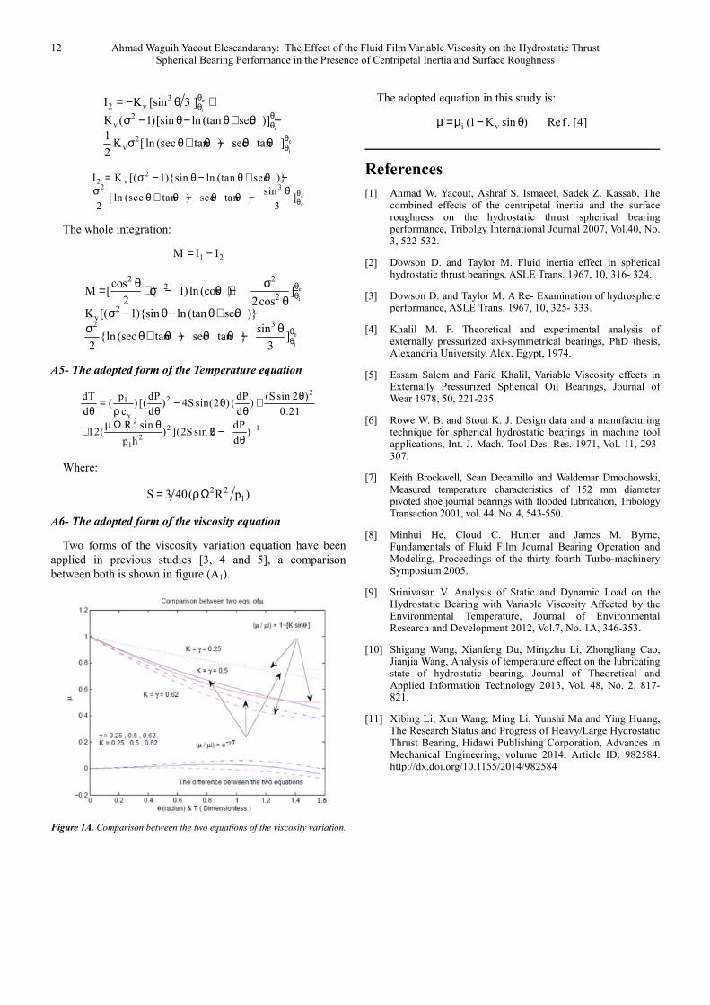
A6- The adopted form of the viscosity equation

Two forms of the viscosity variation equation have been

applied in previous studies [3, 4 and 5], a comparison

between both is shown in figure (A1).

Figure 1A. Comparison between the two equations of the viscosity variation.

The adopted equation in this study is:

i v(1 K sin ) Ref . [4]µ =µ − θ

References

[1] Ahmad W. Yacout, Ashraf S. Ismaeel, Sadek Z. Kassab, The combined effects of the centripetal inertia and the surface roughness on the hydrostatic thrust spherical bearing performance, Tribolgy International Journal 2007, Vol.40, No. 3, 522-532.

[2] Dowson D. and Taylor M. Fluid inertia effect in spherical hydrostatic thrust bearings. ASLE Trans. 1967, 10, 316- 324.

[3] Dowson D. and Taylor M. A Re- Examination of hydrosphere performance, ASLE Trans. 1967, 10, 325- 333.

[4] Khalil M. F. Theoretical and experimental analysis of externally pressurized axi-symmetrical bearings, PhD thesis, Alexandria University, Alex. Egypt, 1974.

[5] Essam Salem and Farid Khalil, Variable Viscosity effects in Externally Pressurized Spherical Oil Bearings, Journal of Wear 1978, 50, 221-235.

[6] Rowe W. B. and Stout K. J. Design data and a manufacturing technique for spherical hydrostatic bearings in machine tool applications, Int. J. Mach. Tool Des. Res. 1971, Vol. 11, 293-307.

[7] Keith Brockwell, Scan Decamillo and Waldemar Dmochowski, Measured temperature characteristics of 152 mm diameter pivoted shoe journal bearings with flooded lubrication, Tribology Transaction 2001, vol. 44, No. 4, 543-550.

[8] Minhui He, Cloud C. Hunter and James M. Byrne, Fundamentals of Fluid Film Journal Bearing Operation and Modeling, Proceedings of the thirty fourth Turbo-machinery Symposium 2005.

[9] Srinivasan V. Analysis of Static and Dynamic Load on the Hydrostatic Bearing with Variable Viscosity Affected by the Environmental Temperature, Journal of Environmental Research and Development 2012, Vol.7, No. 1A, 346-353.

[10] Shigang Wang, Xianfeng Du, Mingzhu Li, Zhongliang Cao, Jianjia Wang, Analysis of temperature effect on the lubricating state of hydrostatic bearing, Journal of Theoretical and Applied Information Technology 2013, Vol. 48, No. 2, 817-821.

[11] Xibing Li, Xun Wang, Ming Li, Yunshi Ma and Ying Huang, The Research Status and Progress of Heavy/Large Hydrostatic Thrust Bearing, Hidawi Publishing Corporation, Advances in Mechanical Engineering, volume 2014, Article ID: 982584. http://dx.doi.org/10.1155/2014/982584

the effect of the fluid film variable viscosity on the...

Documents